Embed Size (px)
Citation preview

Harman Outline 1B CENG 5131 PDF
D. Polynomials (Harman P 160)Review Harman Pages 160-161.
Let a0, a1, . . . , an be n+1 arbitrary numbers with an 6= 0. Then, the function
P (z) = anzn + an−1zn−1 + · · ·+ a0 (1)
is a polynomial of degree n. The n+1 constants a0, a1, . . . , an are the coefficientsof the polynomial. A polynomial is a real polynomial if all its coefficients arereal numbers. This text considers only polynomials with real coefficients unlessotherwise stated, because these are associated with mathematical models ofphysical systems.
The numbers z that are solutions to the equation
P (z) = 0 (2)
are called the roots or sometimes the zeros of the polynomial. The values ofthe roots are not necessarily real numbers. Thus, a root z may have the formz = x + iy, where i is the imaginary number
√−1. In electrical engineering
problems, this is often written j so that no confusion would result with thecurrent if it is designated by i. As described in Chapter 2, the number z̄ = x−iyis the complex conjugate of z. The notation z∗ is also used to designate thecomplex conjugate of z.
1

Important properties of real polynomials and their roots are as follows:
1. A polynomial of degree n ≥ 1 has n roots.
2. A polynomial of odd degree has at least one real root.
3. If z is a complex root of a real polynomial, then the complex conjugate z̄is a root also.
The polynomial P (z) = anzn + an−1zn−1 + · · · + a0 can always be written
in the formP (z) = (z − z1)(z − z2) · · · (z − zn)an (3)
as the product of linear factors using the roots zi, i = 1, 2, . . . , n of
P (z) = 0.
2

MATLAB roots and poly
>> %p= x^3-7x^2+40x-34
>> r=roots([1 -7 40 -34])
r =
3.0000 + 5.0000i3.0000 - 5.0000i1.0000
>> p=poly(r)
p =
1.0000 -7.0000 40.0000 -34.0000
See also conv and deconv Harman p431 and polyval Harmanp350.
Polynomial fit (7.1, P351) Go over Example 7.1 HarmanP353.
3

Handout 4. Functions, Sequences, Series (Harman P 276)Review Harman Pages 276-277,282-296.
1. Continuous functions definition P276
2. Sequences Section 6.2 P 282
3. Infinite Series P 284-287
4. Geometric Series P 287
5. Series of functions P 288
6. Power Series P 290
Taylor Series (6.3, P292)After a review of Taylor series, we can visit Euler’s formula againusing results in Table 6.3 P295. Consider the Taylor series
eiθ = 1 + iθ +(iθ)2
2!+
(iθ)3
3!+
(iθ)4
4!+ · · ·
Collecting terms using the fact that i2 = −1, i3 = −i, and so onyields
eiθ =
(1− (θ)2
2!+
(θ)4
4!− · · ·
)+ i
(θ − (θ)3
3!+
(θ)5
5!− · · ·
)= cos θ + i sin θ (4)
Notice that in all the Taylor series examples, if the argument such asθ in the expansions for sin and cos only a few terms may be neededto satisfy the precision requirements of a problem. For example, ifθ is 0.05 radians (about 3 degrees),
sin(0.05) = 0.0500
to four decimal places. In other words, sin x ≈ x when x is small.
4

Figure 1: Caption for FullWaveRectscan0001
EXAMPLE Series Output of a Full Wave RectifierWhen the diodes are reversed biased by the voltage Vp on the
capacitor, the voltage across the resistor and capacitor are equal sothat
i =v
R= C
dv
dt
The differential equation
dv
dt+
v
CRwith initial conditions v(0) = VP
The solution is v(t) = Vpeλt with λ the solution to the characteristic
equation λ + 1/RC = 0 as described in Harman p216. The decay inthe voltage from the peak is computed by expanding the exponentialand evaluating the first terms at t = T/2 to yield
Vmin = Vp exp( −tRC
) ≈ Vp
(1− T/2
RC
)= Vp
(1− 1
2fRC
)(5)
The figures illustrate the problem. The idea is to determine theripple.
5
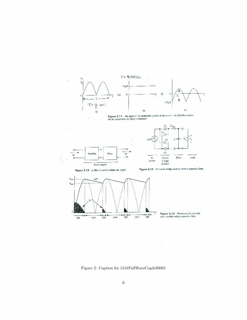
Figure 2: Caption for 5131FullWaveCogdell0001
6

The input wave in is a 120 volt rms, 60 Hertz sine wave so thatv(t) = 120
√2 sin(2π60t). The time constant for the decay is
τ = RC = 100× 2000× 10−6 = 200 ms
which is long compared to the period of the sine wave at T = 1/60 =16.67 ms. Using the values in the series yields a value of about 0.04for the exponent at t = T/2 which indicates that the approximationto Vmin is reasonable.
7
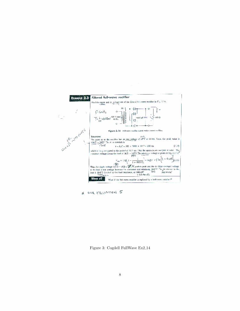
Figure 3: Cogdell FullWave Ex2 14
8