Embed Size (px)
Citation preview


For my precious children, Sarit, Hadas, Efrat, Yair and Tamar,with whom playing has always been so much fun.
And for my beloved wife Michal,soul-mate, playmate, teammate and partner.
(D.H.)
For my dear parents, Terry and Aaron Marelly,who taught me how to play.
And for my beloved wife and daughters, Tali, Noa and Adi,with whom I enjoy playing each and every day.
(R.M.)

Preface
This book does not tell a story. Instead, it is about stories. Or rather, intechnical terms, it is about scenarios. Scenarios of system behavior. It con-centrates on reactive systems, be they software or hardware, or combinedcomputer-embedded systems, including distributed and real-time systems.
We propose a different way to program such systems, centered on inter-object scenario-based behavior. The book describes a language, two tech-niques, and a supporting tool. The language is a rather broad extension oflive sequence charts (LSCs), the original version of which was proposedin 1998 by W. Damm and the first-listed author of this book. The first ofthe two techniques, called play-in, is a convenient way to ‘play in’ scenario-based behavior directly from the system’s graphical user interface (GUI).The second technique, play-out, makes it possible to execute, or ‘play out’,the behavior on the GUI as if it were programmed in a conventional intra-object state-based fashion. All this is implemented in full in our tool, thePlay-Engine.
The book can be viewed as offering improvements in some of the phases ofknown system development life cycles, e.g., requirements capture and anal-ysis, prototyping, and testing. However, there is a more radical way to viewthe book, namely, as proposing an alternative way to program reactivity,which, being based on inter-object scenarios, is a lot closer to how peoplethink about systems and their behavior.
We are excited by the apparent potential of this work. However, whetheror not it is adopted and becomes really useful, what kinds of systems are theideas most fitting for, and how we should develop methodologies for large-scale applications, all remain to a large extent open questions. Whatever thecase, we hope that the book triggers further research and experimentation.
David Harel and Rami MarellyRehovot, February 2003

Note on the Software
The Play-Engine tool is available with the book for free, and the attachedCD contains most of the files needed for using the software. However, someof the ideas behind the play-in and play-out methods are patent-pending,and both the relevant intellectual property and the Play-Engine softwareitself are owned by the Weizmann Institute of Science. In order to ob-tain the remaining parts of the software, please visit the book’s website,www.wisdom.weizmann.ac.il/∼playbook, where you will be asked to signan appropriate license agreement and to register your details.
A reservation is in order here: the Play-Engine is not a commercial product(at least at the time of writing), and should be regarded as a research-leveltool. Thus, its reliability and ease of use are less than what would be expectedfrom professional software, and we cannot be held responsible for its perfor-mance. Nevertheless, we will make an effort to correct bugs and to otherwiseimprove and modify the tool, posting periodical updates on the website. Infact, we have already made some slight changes in the software since thetext of the book was finalized a few weeks ago; these are all documented inthe User Guide that is attached to the software. We would be very gratefulif readers would use the appropriate locations on the website to report anyerrors, both in the software and in the text of the book.
So, please do come and visit the site, sign in, download, play, and enjoy. . .

Acknowledgments
Our first thanks go to Werner Damm from the University of Oldenburg. His1997–98 collaboration with the first-listed author — to which he broughtboth the scientist’s skill and the pragmatist’s insight — yielded the originalversion of the LSCs language, which turned out to be the crucial prerequisiteof our work.
A very special thanks goes to Hillel Kugler and Na’aman Kam for beingsuch demanding, yet tolerant users of the Play-Engine. Many of their com-ments and suggestions have found their way into the material presented here.Hillel’s work on smart play-out (cosupervised by Amir Pnueli) is the mostpromising follow-up research project related to the topic of this book, andwe would like to further thank him for his help in our research on symbolicinstances, and for his dedication in the effort of writing Chap. 18. Na’amanalso supplied the examples from the C. elegans nematode model given in thatchapter.
We received helpful suggestions and insightful comments from severalother people during our work. They include Liran Carmel, Sol Efroni, YaelKfir, Jochen Klose, Yehuda Koren, Anat Maoz, David Peleg, Amir Pnueli,Ehud Shapiro, Gera Weiss and an anonymous referee.
Thanks go to Dan Barak for his work on connecting multiple Play-Engines(the SEC project) and for helping with the implementation of external ob-jects. Evgeniy Bart and Maksim Frenkel helped develop an early version ofGUIEdit.
The first-listed author would also like to thank the Verimag research centerin Grenoble, and its director, Joseph Sifakis, for a generous part-time visitingposition in 2002, during which parts of the book were written.
The second-listed author would like to thank Orna Grumberg and MotiKehat for helping him make the right choices at the right times.
Contents
Part I. Prelude
1. Introduction . . . . . . . . . . . . . . . . . . . . . . . . . . . . . . . . . . . . . . . . . . . . . . 31.1 What Are We Talking About? . . . . . . . . . . . . . . . . . . . . . . . . . . . . 31.2 What Are We Trying to Do? . . . . . . . . . . . . . . . . . . . . . . . . . . . . . 61.3 What’s in the Book? . . . . . . . . . . . . . . . . . . . . . . . . . . . . . . . . . . . . . 7
2. Setting the Stage . . . . . . . . . . . . . . . . . . . . . . . . . . . . . . . . . . . . . . . . . 92.1 Modeling and Code Generation . . . . . . . . . . . . . . . . . . . . . . . . . . . 92.2 Requirements . . . . . . . . . . . . . . . . . . . . . . . . . . . . . . . . . . . . . . . . . . . 122.3 Inter-Object vs. Intra-Object Behavior . . . . . . . . . . . . . . . . . . . . . 142.4 Live Sequence Charts (LSCs) . . . . . . . . . . . . . . . . . . . . . . . . . . . . . 162.5 Testing, Verification and Synthesis . . . . . . . . . . . . . . . . . . . . . . . . 172.6 The Play-In/Play-Out Approach . . . . . . . . . . . . . . . . . . . . . . . . . . 21
3. An Example-Driven Overview . . . . . . . . . . . . . . . . . . . . . . . . . . . . . 253.1 The Sample System . . . . . . . . . . . . . . . . . . . . . . . . . . . . . . . . . . . . . 253.2 Playing In . . . . . . . . . . . . . . . . . . . . . . . . . . . . . . . . . . . . . . . . . . . . . . 263.3 Playing Out . . . . . . . . . . . . . . . . . . . . . . . . . . . . . . . . . . . . . . . . . . . . 393.4 Using Play-Out for Testing . . . . . . . . . . . . . . . . . . . . . . . . . . . . . . . 433.5 Transition to Design . . . . . . . . . . . . . . . . . . . . . . . . . . . . . . . . . . . . . 443.6 Time . . . . . . . . . . . . . . . . . . . . . . . . . . . . . . . . . . . . . . . . . . . . . . . . . . 463.7 Smart Play-Out . . . . . . . . . . . . . . . . . . . . . . . . . . . . . . . . . . . . . . . . . 47
Part II. Foundations
4. The Model: Object Systems . . . . . . . . . . . . . . . . . . . . . . . . . . . . . . . 554.1 Application Types . . . . . . . . . . . . . . . . . . . . . . . . . . . . . . . . . . . . . . . 554.2 Object Properties . . . . . . . . . . . . . . . . . . . . . . . . . . . . . . . . . . . . . . . 564.3 And a Bit More Formally ... . . . . . . . . . . . . . . . . . . . . . . . . . . . . . . 58

XIV Contents
5. The Language: Live Sequence Charts (LSCs) . . . . . . . . . . . . . . 595.1 Constant LSCs . . . . . . . . . . . . . . . . . . . . . . . . . . . . . . . . . . . . . . . . . . 605.2 Playing In . . . . . . . . . . . . . . . . . . . . . . . . . . . . . . . . . . . . . . . . . . . . . . 625.3 The General Play-Out Scheme . . . . . . . . . . . . . . . . . . . . . . . . . . . . 655.4 Playing Out . . . . . . . . . . . . . . . . . . . . . . . . . . . . . . . . . . . . . . . . . . . . 685.5 Combining Locations and Messages . . . . . . . . . . . . . . . . . . . . . . . . 715.6 And a Bit More Formally ... . . . . . . . . . . . . . . . . . . . . . . . . . . . . . . 735.7 Bibliographic Notes . . . . . . . . . . . . . . . . . . . . . . . . . . . . . . . . . . . . . 81
6. The Tool: The Play-Engine . . . . . . . . . . . . . . . . . . . . . . . . . . . . . . . 836.1 Bibliographic Notes . . . . . . . . . . . . . . . . . . . . . . . . . . . . . . . . . . . . . 87
Part III. Basic Behavior
7. Variables and Symbolic Messages . . . . . . . . . . . . . . . . . . . . . . . . . 917.1 Symbolic Scenarios . . . . . . . . . . . . . . . . . . . . . . . . . . . . . . . . . . . . . . 917.2 Enriching the Partial Order . . . . . . . . . . . . . . . . . . . . . . . . . . . . . . 947.3 Playing Out . . . . . . . . . . . . . . . . . . . . . . . . . . . . . . . . . . . . . . . . . . . . 977.4 And a Bit More Formally ... . . . . . . . . . . . . . . . . . . . . . . . . . . . . . . 997.5 Bibliographic Notes . . . . . . . . . . . . . . . . . . . . . . . . . . . . . . . . . . . . . 103
8. Assignments and Implemented Functions . . . . . . . . . . . . . . . . . 1058.1 Using Implemented Functions . . . . . . . . . . . . . . . . . . . . . . . . . . . . . 1058.2 Assignments . . . . . . . . . . . . . . . . . . . . . . . . . . . . . . . . . . . . . . . . . . . . 1088.3 Playing Out . . . . . . . . . . . . . . . . . . . . . . . . . . . . . . . . . . . . . . . . . . . . 1118.4 And a Bit More Formally ... . . . . . . . . . . . . . . . . . . . . . . . . . . . . . . 114
9. Conditions . . . . . . . . . . . . . . . . . . . . . . . . . . . . . . . . . . . . . . . . . . . . . . . . 1199.1 Cold Conditions . . . . . . . . . . . . . . . . . . . . . . . . . . . . . . . . . . . . . . . . . 1199.2 Hot Conditions . . . . . . . . . . . . . . . . . . . . . . . . . . . . . . . . . . . . . . . . . 1209.3 Playing In . . . . . . . . . . . . . . . . . . . . . . . . . . . . . . . . . . . . . . . . . . . . . . 1219.4 Playing Out . . . . . . . . . . . . . . . . . . . . . . . . . . . . . . . . . . . . . . . . . . . . 1269.5 And a Bit More Formally ... . . . . . . . . . . . . . . . . . . . . . . . . . . . . . . 1289.6 Bibliographic Notes . . . . . . . . . . . . . . . . . . . . . . . . . . . . . . . . . . . . . 132
10. Branching and Subcharts . . . . . . . . . . . . . . . . . . . . . . . . . . . . . . . . . 13310.1 The If-Then-Else Construct . . . . . . . . . . . . . . . . . . . . . . . . . . . . . . 13310.2 Subcharts . . . . . . . . . . . . . . . . . . . . . . . . . . . . . . . . . . . . . . . . . . . . . . 13410.3 Nondeterministic Choice . . . . . . . . . . . . . . . . . . . . . . . . . . . . . . . . . 13510.4 Playing In . . . . . . . . . . . . . . . . . . . . . . . . . . . . . . . . . . . . . . . . . . . . . . 13610.5 Playing Out . . . . . . . . . . . . . . . . . . . . . . . . . . . . . . . . . . . . . . . . . . . . 138
Contents XV
10.6 And a Bit More Formally ... . . . . . . . . . . . . . . . . . . . . . . . . . . . . . . 14110.7 Bibliographic Notes . . . . . . . . . . . . . . . . . . . . . . . . . . . . . . . . . . . . . 146
Part IV. Advanced Behavior: Multiple Charts
11. Executing Multiple Charts . . . . . . . . . . . . . . . . . . . . . . . . . . . . . . . . 14911.1 Simultaneous Activation of Multiple Charts . . . . . . . . . . . . . . . . 14911.2 Overlapping Charts . . . . . . . . . . . . . . . . . . . . . . . . . . . . . . . . . . . . . 15411.3 And a Bit More Formally ... . . . . . . . . . . . . . . . . . . . . . . . . . . . . . . 157
12. Testing with Existential Charts . . . . . . . . . . . . . . . . . . . . . . . . . . . 15912.1 Specifying Test Scenarios . . . . . . . . . . . . . . . . . . . . . . . . . . . . . . . . . 15912.2 Monitoring LSCs . . . . . . . . . . . . . . . . . . . . . . . . . . . . . . . . . . . . . . . . 16012.3 Recording and Replaying . . . . . . . . . . . . . . . . . . . . . . . . . . . . . . . . . 16212.4 On-line Testing . . . . . . . . . . . . . . . . . . . . . . . . . . . . . . . . . . . . . . . . . 16412.5 Executing and Monitoring LSCs in the Play-Engine . . . . . . . . . 16512.6 And a Bit More Formally ... . . . . . . . . . . . . . . . . . . . . . . . . . . . . . . 16612.7 Bibliographic Notes . . . . . . . . . . . . . . . . . . . . . . . . . . . . . . . . . . . . . 171
Part V. Advanced Behavior: Richer Constructs
13. Loops . . . . . . . . . . . . . . . . . . . . . . . . . . . . . . . . . . . . . . . . . . . . . . . . . . . . . 17513.1 Using Loops . . . . . . . . . . . . . . . . . . . . . . . . . . . . . . . . . . . . . . . . . . . . 17513.2 Playing In . . . . . . . . . . . . . . . . . . . . . . . . . . . . . . . . . . . . . . . . . . . . . . 17613.3 Playing Out . . . . . . . . . . . . . . . . . . . . . . . . . . . . . . . . . . . . . . . . . . . . 17813.4 Using Variables Within Loops . . . . . . . . . . . . . . . . . . . . . . . . . . . . 17913.5 Executing and Monitoring Dynamic Loops . . . . . . . . . . . . . . . . . 18113.6 And a Bit More Formally ... . . . . . . . . . . . . . . . . . . . . . . . . . . . . . . 18313.7 Bibliographic Notes . . . . . . . . . . . . . . . . . . . . . . . . . . . . . . . . . . . . . 187
14. Transition to Design . . . . . . . . . . . . . . . . . . . . . . . . . . . . . . . . . . . . . . 18914.1 The Design Phase . . . . . . . . . . . . . . . . . . . . . . . . . . . . . . . . . . . . . . . 18914.2 Incorporating Internal Objects . . . . . . . . . . . . . . . . . . . . . . . . . . . . 19014.3 Calling Object Methods . . . . . . . . . . . . . . . . . . . . . . . . . . . . . . . . . . 19314.4 Playing Out . . . . . . . . . . . . . . . . . . . . . . . . . . . . . . . . . . . . . . . . . . . . 19614.5 External Objects . . . . . . . . . . . . . . . . . . . . . . . . . . . . . . . . . . . . . . . . 19814.6 And a Bit More Formally ... . . . . . . . . . . . . . . . . . . . . . . . . . . . . . . 20114.7 Bibliographic Notes . . . . . . . . . . . . . . . . . . . . . . . . . . . . . . . . . . . . . 205

XVI Contents
15. Classes and Symbolic Instances . . . . . . . . . . . . . . . . . . . . . . . . . . . 20915.1 Symbolic Instances . . . . . . . . . . . . . . . . . . . . . . . . . . . . . . . . . . . . . . 20915.2 Classes and Objects . . . . . . . . . . . . . . . . . . . . . . . . . . . . . . . . . . . . . 21015.3 Playing with Simple Symbolic Instances . . . . . . . . . . . . . . . . . . . . 21215.4 Symbolic Instances in the Main Chart . . . . . . . . . . . . . . . . . . . . . 21315.5 Quantified Binding . . . . . . . . . . . . . . . . . . . . . . . . . . . . . . . . . . . . . . 21515.6 Reusing a Scenario Prefix . . . . . . . . . . . . . . . . . . . . . . . . . . . . . . . . 21615.7 Symbolic Instances in Existential Charts . . . . . . . . . . . . . . . . . . . 21815.8 An Advanced Example: NetPhone . . . . . . . . . . . . . . . . . . . . . . . . . 21815.9 And a Bit More Formally ... . . . . . . . . . . . . . . . . . . . . . . . . . . . . . . 22015.10Bibliographic Notes . . . . . . . . . . . . . . . . . . . . . . . . . . . . . . . . . . . . . 227
16. Time and Real-Time Systems . . . . . . . . . . . . . . . . . . . . . . . . . . . . . 22916.1 An Example . . . . . . . . . . . . . . . . . . . . . . . . . . . . . . . . . . . . . . . . . . . . 22916.2 Adding Time to LSCs . . . . . . . . . . . . . . . . . . . . . . . . . . . . . . . . . . . 23016.3 Hot Timing Constraints . . . . . . . . . . . . . . . . . . . . . . . . . . . . . . . . . . 23116.4 Cold Timing Constraints . . . . . . . . . . . . . . . . . . . . . . . . . . . . . . . . . 23416.5 Time Events . . . . . . . . . . . . . . . . . . . . . . . . . . . . . . . . . . . . . . . . . . . . 23516.6 Playing In . . . . . . . . . . . . . . . . . . . . . . . . . . . . . . . . . . . . . . . . . . . . . . 23616.7 Playing Out . . . . . . . . . . . . . . . . . . . . . . . . . . . . . . . . . . . . . . . . . . . . 23716.8 Unification of Clock Ticks . . . . . . . . . . . . . . . . . . . . . . . . . . . . . . . . 23916.9 The Time-Enriched NetPhone Example . . . . . . . . . . . . . . . . . . . . 24016.10And a Bit More Formally ... . . . . . . . . . . . . . . . . . . . . . . . . . . . . . . 24216.11Bibliographic Notes . . . . . . . . . . . . . . . . . . . . . . . . . . . . . . . . . . . . . 247
17. Forbidden Elements . . . . . . . . . . . . . . . . . . . . . . . . . . . . . . . . . . . . . . . 25117.1 Example: A Cruise Control System . . . . . . . . . . . . . . . . . . . . . . . . 25117.2 Forbidden Messages . . . . . . . . . . . . . . . . . . . . . . . . . . . . . . . . . . . . . 25217.3 Generalized Forbidden Messages . . . . . . . . . . . . . . . . . . . . . . . . . . 25517.4 Symbolic Instances in Forbidden Messages . . . . . . . . . . . . . . . . . . 25617.5 Forbidden Conditions . . . . . . . . . . . . . . . . . . . . . . . . . . . . . . . . . . . . 25817.6 Scoping Forbidden Elements . . . . . . . . . . . . . . . . . . . . . . . . . . . . . . 26217.7 Playing Out . . . . . . . . . . . . . . . . . . . . . . . . . . . . . . . . . . . . . . . . . . . . 26417.8 Using Forbidden Elements with Time . . . . . . . . . . . . . . . . . . . . . . 26617.9 A Tolerant Semantics for LSCs. . . . . . . . . . . . . . . . . . . . . . . . . . . . 26617.10And a Bit More Formally ... . . . . . . . . . . . . . . . . . . . . . . . . . . . . . . 26817.11Bibliographic Notes . . . . . . . . . . . . . . . . . . . . . . . . . . . . . . . . . . . . . 278
Part VI. Enhancing the Play-Engine

Contents XVII
18. Smart Play-Out (with H. Kugler) . . . . . . . . . . . . . . . . . . . . . . . 28118.1 Introduction . . . . . . . . . . . . . . . . . . . . . . . . . . . . . . . . . . . . . . . . . . . . 28118.2 Being Smart Helps . . . . . . . . . . . . . . . . . . . . . . . . . . . . . . . . . . . . . . 28318.3 The General Approach . . . . . . . . . . . . . . . . . . . . . . . . . . . . . . . . . . . 28718.4 The Translation . . . . . . . . . . . . . . . . . . . . . . . . . . . . . . . . . . . . . . . . . 28918.5 Current Limitations . . . . . . . . . . . . . . . . . . . . . . . . . . . . . . . . . . . . . 29918.6 Satisfying Existential Charts . . . . . . . . . . . . . . . . . . . . . . . . . . . . . 30118.7 Bibliographic Notes . . . . . . . . . . . . . . . . . . . . . . . . . . . . . . . . . . . . . 307
19. Inside and Outside the Play-Engine . . . . . . . . . . . . . . . . . . . . . . . 30919.1 The Engine’s Environment . . . . . . . . . . . . . . . . . . . . . . . . . . . . . . . 30919.2 Playing In . . . . . . . . . . . . . . . . . . . . . . . . . . . . . . . . . . . . . . . . . . . . . . 31019.3 Playing Out . . . . . . . . . . . . . . . . . . . . . . . . . . . . . . . . . . . . . . . . . . . . 31119.4 Recording Runs and Connecting External Applications . . . . . . . 31319.5 Additional Play-Engine Features . . . . . . . . . . . . . . . . . . . . . . . . . . 313
20. A Play-Engine Aware GUI Editor . . . . . . . . . . . . . . . . . . . . . . . . . 31720.1 Who Needs a GUI Editor? . . . . . . . . . . . . . . . . . . . . . . . . . . . . . . . 31720.2 GUIEdit in Visual Basic . . . . . . . . . . . . . . . . . . . . . . . . . . . . . . . . . 31820.3 What Does GUIEdit Do? . . . . . . . . . . . . . . . . . . . . . . . . . . . . . . . . 31820.4 Incorporating Custom Controls . . . . . . . . . . . . . . . . . . . . . . . . . . . 32120.5 GUIEdit As a Proof of Concept . . . . . . . . . . . . . . . . . . . . . . . . . . . 32220.6 Bibliographic Notes . . . . . . . . . . . . . . . . . . . . . . . . . . . . . . . . . . . . . 322
21. Future Research Directions . . . . . . . . . . . . . . . . . . . . . . . . . . . . . . . 32521.1 Object Refinement and Composition . . . . . . . . . . . . . . . . . . . . . . . 32521.2 Object Model Diagrams, Inheritance and Interfaces . . . . . . . . . . 32721.3 Dynamic Creation and Destruction of Objects . . . . . . . . . . . . . . 32821.4 Structured Properties and Types . . . . . . . . . . . . . . . . . . . . . . . . . . 32921.5 Linking Multiple Engines . . . . . . . . . . . . . . . . . . . . . . . . . . . . . . . . . 330
Part VII. Appendices
A. Formal Semantics of LSCs . . . . . . . . . . . . . . . . . . . . . . . . . . . . . . . . 335A.1 System Model and Events . . . . . . . . . . . . . . . . . . . . . . . . . . . . . . . . 335A.2 LSC Specification . . . . . . . . . . . . . . . . . . . . . . . . . . . . . . . . . . . . . . . 338A.3 Operational Semantics . . . . . . . . . . . . . . . . . . . . . . . . . . . . . . . . . . . 344
B. XML Description of a GUI Application . . . . . . . . . . . . . . . . . . . 359

XVIII Contents
C. The Play-Engine Interface . . . . . . . . . . . . . . . . . . . . . . . . . . . . . . . . 363C.1 Visual Basic Code . . . . . . . . . . . . . . . . . . . . . . . . . . . . . . . . . . . . . . . 363
D. The GUI Application Interface . . . . . . . . . . . . . . . . . . . . . . . . . . . . 365D.1 Visual Basic Code . . . . . . . . . . . . . . . . . . . . . . . . . . . . . . . . . . . . . . . 366
E. The Structure of a (Recorded) Run . . . . . . . . . . . . . . . . . . . . . . . 369
References . . . . . . . . . . . . . . . . . . . . . . . . . . . . . . . . . . . . . . . . . . . . . . . . . . . . 371
Index . . . . . . . . . . . . . . . . . . . . . . . . . . . . . . . . . . . . . . . . . . . . . . . . . . . . . . . . . 377

Part I
Prelude


1. Introduction
1.1 What Are We Talking About?
What kinds of systems are we interested in? Well, first and foremost, we havein mind computerized and computer embedded systems, mainly those thatare reactive in nature. For these reactive systems, as they are called, thecomplexity we have to deal with does not stem from complex computationsor complex data, but from intricate to-and-from interaction — between thesystem and its environment and between parts of the system itself.
Interestingly, reactivity is not an exclusive characteristic of man-madecomputerized systems. It occurs also in biological systems, which, despitebeing a lot smaller than us humans and our homemade artifacts, can also bea lot more complicated, and it also occurs in economic and social systems,which are a lot larger than a single human. Being able to fully understand andanalyze these kinds of systems, and possibly to predict their future behavior,involves the same kind of thinking required for computerized reactive systems.
When people think about reactive systems, their thoughts fall very natu-rally into the realm of scenarios of behavior. You do not find too many peo-ple saying things like “Well, the controller of my ATM can be in waiting-for-user-input mode or in connecting-to-bank-computer mode or in delivering-money mode; in the first case, here are the possible inputs and the ATM’sreactions, . . .; in the second case, here is what happens, . . ., etc.”. Rather,you find them saying things like “If I insert my card, and then press thisbutton and type in my PIN, then the following shows up on the display, andby pressing this other button my account balance will show”. In other words,it has always been a lot more natural to describe and discuss the reactivebehavior of a system by the scenarios it enables rather than by the state-based reactivity of each of its components. This is particularly true of someof the early and late stages of the system development process — e.g., duringrequirements capture and analysis, and during testing and maintenance —and is in fact what underlies the early stage use case approach. On the otherhand, it seems that in order to implement the system, as opposed to stat-ing its required behavior or preparing test suites, state-based modeling is

4 1. Introduction
needed, whereby we must specify for each component the complete array ofpossibilities for incoming events and changes and the component’s reactionsto them.
This is, in fact, an interesting and subtle duality. On the one hand, wehave scenario-based behavioral descriptions, which cut across the boundariesof the components (or objects) of the system, in order to provide coherent andcomprehensive descriptions of scenarios of behavior. A sort of inter-object,‘one story for all relevant objects’ approach. On the other hand, we have state-based behavioral descriptions, which remain within the component, or object,and are based on providing a complete description of the reactivity of eachone. A sort of intra-object, ‘all pieces of stories for one object’ approach.The former is more intuitive and natural for humans to grasp and is thereforefitting in the requirements and testing stages. The second approach, however,has always been the one needed for implementation; after all, implementinga system requires that each of the components or objects is supplied with itscomplete reactivity, so that it can actually run, or execute. You can’t capturethe entire desired behavior of a complex system by a bunch of scenarios. Andeven if you could, it wouldn’t be at all clear how you could execute such aseemingly unrelated collection of behaviors in an orderly fashion. Figure 1.1visualizes these two approaches.
This duality can also be explained in day-to-day terms. It is like thedifference between describing the game of soccer by specifying the completereactivity of each player, of the ball, of the goal’s wooden posts, etc., vs.specifying the possible scenarios of play that the game supports. As anotherexample, suppose we wanted to describe the ‘behavior’ of some companyoffice. It would be a lot more natural to describe the inter-object scenarios,such as how an employee mails off 50 copies of a document (this could involvethe employee, the secretary, the copy machine, the mail room, etc.), how theboss arranges a conference call with the project managers, or how informationon vacation days and sick leave is organized and forwarded to the payrolloffice. Contrast this with the intra-object style, whereby we would have toprovide complete information on the modes of operation and reactivity of theboss, the secretary, the employees, the copy machine, the mail room, etc.
We are not claiming that scenario-based behavior is technically superiorin some global sense, only that it is a lot more natural. In fact, now is a goodtime to mention that mere isolated scenarios of behavior that the systemcan possibly give rise to are far from adequate. In order to get significantmileage out of scenario-based behavior, we need to be able to attach variousmodalities to the scenarios we are specifying. We would like to distinguishbetween scenarios that may occur and those that must, between those thatoccur spontaneously and those that need some trigger to cause them to occur.

1.1 What Are We Talking About? 5
Fig. 1.1. Inter-object vs. intra-object behavior
We would like to be able to specify multiple scenarios that combine with eachother, or even with themselves, in subtle sequential and/or concurrent ways.We want generic scenarios that can be instantiated by different objects ofthe same class, we want to be able to use variables to store and retrievevalues, and we want means for specifying time. Significantly, we would alsolike to be able to specify anti-scenarios, i.e., ones that are forbidden, in thesense that if they occur there is something very wrong: either something inthe specification is not as we wanted, or else the implementation does notcorrectly satisfy the specification.
Obviously, it would also be very nice if we could actually ‘see’ scenario-based behavior in operation, before (or instead of?) spending lots of time,energy and money on intra-object state-based modeling that leads to theimplementation. In other words, we could do with an approach to inter-objectbehavior that is expressive, natural and executable.
This is what the book is about.

6 1. Introduction
1.2 What Are We Trying to Do?
We propose a powerful setup, within which one can conveniently capturescenario-based behavior, and then execute it and simulate the system underdevelopment exactly as if it were specified in the conventional state-basedfashion. Our work involves a language, two techniques with detailed under-lying algorithms, and a tool. The entire approach is made possible by thelanguage of live sequence charts, or LSCs, which is extended here in anumber of ways, resulting in a highly expressive medium for scenario-basedbehavior. The first of our two techniques involves a user-friendly and natu-ral way to play in scenario-based behavior directly from the system’s GUI(or some abstract version thereof, such as an object-model diagram), duringwhich LSCs are generated automatically. The second technique, which weconsider to be the technical highlight of our work, makes it possible to playout the behavior, that is, to execute the system as constrained by the grandsum of the scenario-based information. These ideas are supported in full byour tool — the Play-Engine.
There are essentially two ways to view this book. The first — the moreconservative one — is to view it as offering improvements to the various stagesof accepted life-cycles for system development: a more convenient way to cap-ture behavioral requirements, the ability to express more powerful scenario-based behavior, a fully worked-out formalization of use cases, a means forexecuting use cases and their instantiations, tools for the dynamic testing ofrequirements prior to building the actual system model or implementation, ahighly expressive medium for preparing test suites, and a means for testingsystems by dynamic and run-time comparison of two dual-view executables.
The second way to view our work is less conservative. It calls for consid-ering the possibility of an alternative way of programming the behavior of areactive system, which is totally scenario-based and inter-object in nature.Basic to this is the idea that LSCs can actually constitute the implementa-tion of a system, with the play-out algorithms and the Play-Engine being asort of ‘universal reactive mechanism’ that executes the LSCs as if they con-stituted a conventional implementation. If one adopts this view, behavioralspecification of a reactive system would not have to involve any intra-objectmodeling (e.g., in languages like statecharts) or code.
This of course is a more outlandish idea, and still requires that a num-ber of things be assessed and worked out in more detail for it to actuallybe feasible in large-scale systems. Mainly, it requires that a large amount ofexperience and modeling wisdom be accumulated around this new way ofspecifying executable behavior. Still, we see no reason why this ambitiouspossibility should not be considered as it is now. Scenario-based behavior is
1.3 What’s in the Book? 7
what people use when they think about their systems, and our work showsthat it is possible to capture a rich spectrum of such behavior conveniently,and to execute it directly, resulting in a runnable artifact that is as powerfulas an intra-object model. From the point of view of the user, executing suchbehavior looks no different from executing any system model. Moreover, itis hard to underestimate the advantages of having the behavior structuredaccording to the way the engineers invent and design it and the users compre-hend it (for example, in the testing, maintenance and modifications stages, insharing the specification process with less technically oriented people, etc.).
In any case, the book concentrates on describing and illustrating the ideasand technicalities themselves, and not on trying to convince the reader of thisor that usage thereof. How, in what role, and to what extent these ideas willindeed become useful are things that remain to be seen.
1.3 What’s in the Book?
Besides this brief introductory chapter, Part I of the book, the Prelude, con-tains a chapter providing the background and context for the rest of thebook, followed by a high-level overview of the entire approach, from whichthe reader can get a pretty good idea of what we are doing.
Part II, Foundations, describes the underlying basics of the object model,the LSCs language and the Play-Engine tool.
Parts III, IV and V treat in more detail the constructs of the enrichedlanguage of LSCs, and the way they are played in and played out. Almostevery chapter in these three parts contains a section named “And a BitMore Formally . . .”, which provides the syntax and operational semanticsfor the constructs described in the chapter. As we progress from chapter tochapter, we use a blue/black type convention to highlight the additions to,and modifications of, this formal description. (Appendix A contains the fullyaccumulated syntax and semantics.)
Part VI describes extensions and enhancements, with chapters on theinnards of the Play-Engine tool, particularly the play-out algorithms, on theGUI editor we have built to support the construction of application GUIs, onthe smart play-out module, which uses formal verification techniques to driveparts of the execution, and on future research and development directions.
Part VII contains several technical appendices, one of which is the fullformal definition of the enriched LSCs language.


2. Setting the Stage
In this chapter we set the stage for the rest of the book, by describing someof the main ideas in systems and software engineering research that leadto the material developed later. We discuss visual formalisms and model-ing languages, model execution and code generation, the connection betweenstructure and behavior, and the difference between implementable behav-ior and behavioral requirements. We then go on to describe in somewhatmore detail some of the basic concepts we shall be expanding upon, suchas the inter-/intra-object dichotomy, MSCs vs. LSCs, the play-in and play-out techniques, and the way all these fit into our global view of the systemdevelopment process.
2.1 Modeling and Code Generation
Over the years, the main approaches to high-level system modeling havebeen structured-analysis and structured-design (SA/SD), and object-oriented analysis and design (OOAD). The two are about a decade apartin initial conception and evolution. Over the years, both approaches haveyielded visual formalisms for capturing the various parts of a system model,most notably its structure and behavior. A recent book, [120], nicely surveysand discusses some of these approaches.
SA/SD, which started in the late 1970s, is based on raising classic pro-cedural programming concepts to the modeling level and using diagrams formodeling system structure. Structural models are based on functional de-composition and the flow of information, and are depicted using hierarchi-cal dataflow diagrams. Many methodologists were instrumental in setting theground for the SA/SD paradigm, by devising the functional decompositionand dataflow diagram framework, including DeMarco [31], and Constantineand Yourdon [25]. Parnas’s work over the years was very influential too.
In the mid-1980s, several methodology teams enriched this basic SA/SDmodel by providing a way to add state-based behavior to these efforts, us-ing state diagrams or the richer language of statecharts (see Harel [42]).

10 2. Setting the Stage
These teams were Ward and Mellor [117], Hatley and Pirbhai [54], and theStatemate team [48]. A state diagram or statechart is associated with eachfunction or activity, describing its behavior. Several nontrivial issues hadto be worked out to properly connect structure with behavior, enabling themodeler to construct a comprehensive and semantically rigorous model of thesystem; it is not enough to simply decide on a behavioral language and thenassociate each function or activity with a behavioral description.1 The threeteams struggled with this issue, and their decisions on how to link structurewith behavior ended up being very similar. Careful behavioral modeling andits close linking with system structure are especially crucial for reactivesystems [52, 93], of which real-time systems are a special case.
The first commercial tool to enable model execution and full code gen-eration from high-level models was Statemate, built by I-Logix and releasedin 1987 [48, 60]. (Incidentally, the code generated need not necessarily resultin software; it could be code in a hardware description language, leading tohardware.) A detailed summary of the SA/SD languages for structure andbehavior, their relationships and the way they are embedded in the Statematetool appears in [53].
Of course, modelers need not adopt state machines or statecharts to de-scribe behavior. There are many other possible choices, and these can also belinked with the SA/SD functional decomposition. They include such visualformalisms as Petri nets [101] or SDL diagrams [110], more algebraic oneslike CSP [59] or CCS [88], and ones that are closer in appearance to pro-gramming languages, like Esterel [14] and Lustre [41]. Clearly, if one doesnot want to use any such high-level formalisms, code in an appropriate con-ventional programming language could be written directly in order to specifythe behavior of a function in an SA/SD decomposition.
The late 1980s saw the first proposals for object-oriented analysis and de-sign (OOAD). Just like in the SA/SD approach, here too the basic ideain modeling system structure was to lift concepts up from the program-ming level — in this case object-oriented programming — to the modelinglevel and to use visual formalisms. Inspired by entity-relationship (ER)diagrams [21], several methodology teams recommended various forms ofclass diagrams and object model diagrams for modeling system struc-ture [16, 26, 105, 111]. To model behavior, most object-oriented modelingapproaches also adopted statecharts [42]. Each class is ‘programmed’ using astatechart, which then serves to describe the behavior of any instance objectof that class; see, e.g., [105, 16, 44].1 This would be like saying that when you build a car all you need are the structural
things — body, chassis, wheels, etc. — and an engine, and you then merely stick theengine under the hood and you are done.

2.1 Modeling and Code Generation 11
In the OOAD world, the issue of connecting structure and behavior issubtler and a lot more complicated than in the SA/SD one. Classes representdynamically changing collections of concrete objects. Behavioral modelingmust thus address issues related to object creation and destruction, messagedelegation, relationship modification and maintenance, aggregation, inheri-tance, and so on. The links between behavior and structure must be definedin sufficient detail and with enough rigor to support the construction of toolsthat enable model execution and full code generation. See Fig. 2.1.
Fig. 2.1. Object-oriented system modeling with code generation
Obviously, if we have the ability to generate full code, we would eventuallywant that code to serve as the basis for the final implementation. In theOOAD world, a few tools have been able to do this. One is Rhapsody, alsofrom I-Logix [60], which is based on the work of Harel and Gery in [44] onexecutable object modeling with statecharts. Another is ObjectTime, whichis based on the ROOM method of Selic et al. [111], and is now part of theRose RealTime tool from Rational [100]. There is no doubt that techniquesfor this kind of ‘super-compilation’ from high-level visual formalisms downto programming languages will improve in time. Providing higher levels ofabstraction with automated downward transformations has always been theway to go, as long as the abstractions are ones with which the engineers whodo the actual work are happy.

12 2. Setting the Stage
In 1997, the Object Management Group (OMG) adopted as a standardthe unified modeling language (UML), put together by a large team led byBooch, Rumbaugh and Jacobson; see [115, 106]. The class/object diagrams,adapted from the Booch method [16] and the OMT (object modeling tech-nique) method [105], and driven by statecharts for behavior [44], constitutethat part of the UML that specifies unambiguous, executable (and thereforeimplementable) models. It has been termed XUML, for executable UML.The UML also has several means for specifying more elaborate aspects ofsystem structure and architecture (for example, packages and components).Large amounts of further information on the UML can be found in OMG’swebsite [115].
2.2 Requirements
So much for modeling systems in the SA/SD and OO worlds. However, theimportance of executable models lies not only in their ability to help lead toa final implementation, but also in testing and debugging, the basis of whichare the requirements. These constitute the constraints, desires, dreams andhopes we entertain concerning the behavior of the system under development.We want to make sure, both during development and when we feel develop-ment is over, that the system does, or will do, what we intend or hope for itto do.
Requirements can be formal (rigorously and precisely defined) or infor-mal (written, say, in natural language or pseudocode). An interesting wayto describe high-level behavioral requirements is the idea of use cases; seeJacobson [62]. A use case is an informal description of a collection of possiblescenarios involving the system under discussion and its external actors. Usecases describe the observable reactions of a system to events triggered by itsusers. Usually, the description of a use case is divided into the main, most fre-quently used scenario, and exceptional scenarios that give rise to less centralbehaviors branching out from the main one (e.g., possible errors, cancellingan operation before completion, etc.). However, since use cases are high-leveland informal by nature, they cannot serve as the basis for formal testing andverification. To support a more complete and rigorous development cycle,use cases must be translated into fully detailed requirements written in someformal language.
Ever since the early days of high-level programming, computer scienceresearchers have grappled with requirements; namely, with how to best statewhat we want of a complex program or system. Notable efforts are those em-bodied in the classic Floyd/Hoare inductive assertions method, which uses

2.2 Requirements 13
invariants, pre- and post-conditions and termination statements [12], and inthe many variants of temporal logic [82]. These make it possible to expressdifferent kinds of requirements that are of interest in reactive systems. Theyinclude safety constraints, which state that bad things will not happen;for example, this program will never terminate with the wrong answer, orthis elevator door will never open between floors. They also include livenessconstraints, which state that good things must happen. For example, thisprogram will eventually terminate, or this elevator will open its door on thedesired floor within the allotted time limit.
A more recent way to specify requirements, which is popular in the realmof object-oriented systems, is to use message sequence charts (MSCs),which are used to specify scenarios as sequences of message interactions be-tween object instances. This visual language was adopted as a standard longago by the International Telecommunication Union (the ITU; formerly theCCITT) [123], and it also manifests itself in the UML as the language ofsequence diagrams (see [115]). MSCs combine nicely with use cases, sincethey can specify the scenarios that instantiate the use cases. Sequence chartsthus capture the desired interrelationships between the processes, tasks, com-ponents or object instances — and between them and the environment — ina way that is linear or quasilinear in time.2 In other words, the modeler usesMSCs to formally visualize the actual scenarios that the more abstract andgeneric use cases were intended to denote.
Objects in MSCs are represented by vertical lines, and messages betweenthese instances are represented by horizontal (or sometimes down-slanted)arrows. Conditional guards, showing up as elongated hexagons, specify state-ments that are to be true when reached. The overall effect of such a chartis to specify a scenario of behavior, consisting of messages flowing betweenobjects and things having to be true along the way.
Figure 2.2 shows a simple example of an MSC for the quick-dial featureof a cellular telephone. The sequence of messages it depicts consists of thefollowing: the user clicks the ∗ key, and then clicks a digit on the Keyboard,followed by the Send Key, which sends a Sent indication to the internal Chip.The Chip, in turn, sends the digit to the Memory to retrieve the telephonenumber associated with the clicked digit, and then sends out the number tothe external Environment to carry out a call. A signal is then received fromthe environment, guarded by a condition asserting that it is not a busy signal.2 Tasks, processes and components are mentioned here too, since although the book is
couched in the terminology of object-orientation, many of the ideas apply also to otherways of structuring systems.

14 2. Setting the Stage
Fig. 2.2. A message sequence chart (MSC)
2.3 Inter-Object vs. Intra-Object Behavior
The style of behavior captured by sequence charts is inter-object, to be con-trasted with the intra-object style of statecharts. Whereas a sequence chartcaptures what goes on in a scenario of behavior that takes place betweenand amongst the objects, a statechart captures the full behavioral specifica-tion for one of those objects (or tasks or processes). Statecharts thus providedetails of an object’s behavior under all possible conditions and in all thepossible ‘stories’ described previously in the inter-object sequence charts.
Two points must now be made regarding sequence charts. The first is oneof exposition: by and large, the subtle difference in the roles of sequence-basedlanguages for behavior and component-based ones is not made clear in theliterature. Again and again, one comes across articles and books (many ofthem related to UML) in which the very same phrases are used to introducesequence diagrams and statecharts. At one point such a publication might saythat “sequence diagrams can be used to specify behavior”, and later it mightsay that “statecharts can be used to specify behavior”. Sadly, the reader istold nothing about the fundamental difference in nature and usage betweenthe two — that one is a medium for conveying requirements, i.e., the inter-object behavior required of a model, and the other is part of the executablemodel itself. This obscurity is one of the reasons many naive readers comeaway confused by the multitude of diagram types in the full UML standardand the lack of clear recommendations about what it means to specify thebehavior of a system in a way that can be implemented and executed.

2.3 Inter-Object vs. Intra-Object Behavior 15
The second point is more substantial. As a requirements language, themany variants of MSCs, including the ITU standard [124] and the sequencediagrams adopted in the UML [115], as well as versions enriched with timingconstraints and co-regions, and the high-level MSCs that make it possibleto combine charts using the power of regular expressions, have very limitedexpressive power. Their semantics is intended to support the specificationof possible scenarios of system behavior, and is therefore usually given by aset of simple constraints on the partial order of possible events in a systemexecution: along a vertical object line higher events precede lower ones, andthe sending of a message precedes its receipt.3 Virtually nothing can be saidin such diagrams about what the system will actually do when run. Theycan state what might possibly occur, not what must occur. In the chart ofFig. 2.2, for example, there is nothing to indicate whether some parts ofthe scenario are mandatory. For example, can the Memory ‘decide’ not tosend back a number in response to the request from the Chip? Does theguarding condition stating that the signal is not busy really have to be true?What happens if it is not? If one wants to be puristic, then, under mostdefinitions of the semantics of message sequence charts, an empty system— one that doesn’t do anything in response to anything — satisfies such achart. Hence, just sitting back and doing nothing will make your requirementshappy. (Usually, however, there is a minimal, often implicit, requirement thateach one of the specified sequence charts should have at least one run of thesystem that winds its way correctly through it.)
MSCs can be used to specify expected scenarios of behavior in the re-quirements stage, and can be used as test scenarios that will be later checkedagainst the executing behavior of the final system. However, they are notenough if we want to specify the actual behavior of a reactive system in ascenario-based fashion. We would like to be able to say what may happenand what must happen, and also what is not allowed to happen. The lattergives rise to what we call anti-scenarios, in the sense that if they occursomething is very wrong: either something in the specification is not as wewanted, or else the implementation does not correctly satisfy the specifica-tion. We would like to be able to specify multiple scenarios that combinewith each other, or even with themselves, in subtle ways. We want to be ableto specify generic scenarios, i.e., ones that stand for many specific scenar-ios, in that they can be instantiated by different objects of the same class.We want variables and means for specifying real time, and so on.3 There can also be synchronous messages, for which the two events are simultaneous.

16 2. Setting the Stage
2.4 Live Sequence Charts (LSCs)
In 1998 Damm and Harel addressed many of these deficiencies, resulting inan extension of MSCs, called live sequence charts (or LSCs); see [27].The name comes from the ability to specify liveness, i.e., things that mustoccur. Technically, LSCs allow a distinction between possible and necessarybehavior, both globally, on the level of an entire chart, and locally, whenspecifying events, guarding conditions, and progress over time within a chart.
LSCs have two types of charts: universal (enclosed within a solid bor-derline) and existential (enclosed within a dashed borderline). Universalcharts are the more interesting ones, and are used to specify scenario-basedbehavior that applies to all possible system runs. A universal chart has twoparts, turning it into a kind of if-then construct.4 It has a prechart thatspecifies the scenario that, if satisfied, forces the system to also satisfy theactual chart body, the main chart. Thus, such an LSC induces an action-reaction relationship between the scenario appearing in its prechart and theone appearing in the chart body. Taken together, a collection of LSCs pro-vides a set of action-reaction pairs of scenarios, and the universal ones mustbe satisfied at all times during any system run.
Fig. 2.3. A live sequence chart (LSC)
4 This structure is actually very much like a [α]〈β〉true construct in dynamic logic, eval-uated in each system run.

2.5 Testing, Verification and Synthesis 17
Within a chart, the live elements, termed hot, signify things that mustoccur, and they can be used to specify various modalities of behavior, in-cluding anti-scenarios. The other elements, termed cold, signify things thatmay occur, and they can be used to specify control structures like branch-ing and iteration. In subsequence chapters we will see numerous examples ofthe expressive power of these two kinds of elements, and the subtlety of thedifferences between them.
Figure 2.3 shows a universal LSC that is an enriched version of the MSCin Fig. 2.2. The first three events are in the prechart, and the others are in themain chart. Hence, the LSC states that whenever the user clicks ∗, followed bya digit, followed by the Send Key, the rest of the scenario must be satisfied.The messages in the main chart are hot (depicted by solid red arrows, incontrast to the dashed blue ones in the prechart), as are the vertical lines.Thus progress along all lines in the main chart must occur and the messagesmust be sent and received in order for the chart to be satisfied. In addition,a loop has been added, within which the chip can make up to three attemptsto get a non-busy signal from the environment.
The loop is controlled by the cold (blue dashed line) guarding condition,which means that as long as the signal is busy the 3-round loop continues.The semantics of a cold condition, however, is such that if it is false nothingbad has happened, and execution simply moves up one level, out of theinnermost chart or subchart. In our case, if the signal is not busy the loopis exited (which means that the entire chart has been satisfied). In contrastto this, a hot condition must be true when reached during a system run, andif it is not the system must abort, since this is an unforgivable error. Oneway to specify an anti-scenario using hot conditions (e.g., an elevator dooropening when it shouldn’t, or a missile firing when the radar is not lockedon the target) is to include the entire unwanted scenario in the prechart,followed by a main chart that contains a single false hot condition.
2.5 Testing, Verification and Synthesis
Since they are more expressive than MSCs,5 LSCs also make it possible tohave a closer look at the aforementioned dichotomy of reactive behavior,namely, the relationship between the inter-object requirements view and theintra-object implementable model view.
If we now extend Fig. 2.1, adding to it the requirements, we obtain Fig.2.4. Its right-hand side is the implementable intra-object system model, which5 The expressive power of LSCs is actually very close to that of statecharts as embedded
in the object-oriented paradigm — what we called earlier XUML.

18 2. Setting the Stage
leads to the final software or hardware, and will consist of the complete be-havior coded for each object. In contrast, it is common to assume that theleft-hand side, the set of requirements, is not implementable or executable. Acollection of scenarios cannot be considered an implementable model of thesystem: How would such a system operate? What would it do under generaldynamic circumstances? How would we decide what scenarios would be rele-vant when some event suddenly occurs out of the blue? How should we dealwith the mandatory, the possible and the forbidden, during execution? Andhow would we know what subsequent behaviors these and other modalitiesof behavior might entail?
Fig. 2.4. Conventional system development
One of the main messages of this book is that this assumption is no longervalid. Scenario-based behavior need not be limited to requirements that willbe specified before the real executable system is built and will then be usedmerely to test that system. Scenario-based behavior, we claim, can actuallybe executed. Furthermore, we predict that in many cases such behavior willbecome the implemented system itself. This will be illustrated and discussedin detail as the book progresses.
For now, let us discuss the relations and transitions between the differentparts of the conventional setup of system development, as shown in Fig. 2.4.The arrow between the use cases and the requirements is dashed for a reason:it does not represent a ‘hard’ computerized process. Going from use cases to

2.5 Testing, Verification and Synthesis 19
formal requirements is a ‘soft’ methodological process performed manually bysystem designers and engineers. It is considered an art or a craft and requiresa good understanding of the target formal requirements language and a largeamount of creativity.
The arrow going from the system model to the requirements depicts test-ing and verifying the model against the requirements. Here is a nice way todo testing using an automated tool.6 Assume the user has specified the re-quirements as a set of sequence diagrams, perhaps instantiating previouslyprepared use cases. For simplicity, let us say that this results in a diagramcalled A. Later, when the executable intra-object system model has beenspecified, the user can execute it and ask that during execution the systemshould automatically construct an animated sequence diagram, call it B, onthe fly. This diagram will show the dynamics of object interaction as it ac-tually happens during execution. When this execution is completed, the toolcan be asked to compare diagrams A and B, and to highlight any inconsisten-cies, such as contradictions in the partial order of events, or events appearingin one diagram but not in the other. In this way, the tool helps debug thebehavior of the system against the requirements.
A recently developed tool, called TestConductor, which is integrated intoRhapsody [60], enables a richer kind of testing using a subset of LSCs. Thetest scenarios can describe scenarios of interaction between the environmentand the system under development. The tool then runs the tests, and simu-lates the behavior of the environment by monitoring the test scenarios andsending messages to the system on behalf of the environment, when required.The tool determines the results of such a test by comparing the sequence dia-grams produced by the system with those that describe the tests using visualcomparison, as described above.
Note that even these powerful ways to check the behavior of a systemmodel against our expectations are limited to those executions that we actu-ally carry out. They thus suffer from the same drawbacks as classic testingand debugging. Since a system can have an infinite number of runs, somewill always go unchecked, and it could be those that violate the requirements(in our case, by being inconsistent with diagram A). As Dijkstra famouslyput it years ago, “testing and debugging cannot be used to demonstrate theabsence of errors, only their presence”.
One remedy is to use true verification. This is not what CASE-tool peoplein the 1980s often called “validation and verification”, which amounted tolittle more than checking the consistency of the model’s syntax. What wehave in mind is a mathematically rigorous and precise proof that the model6 Rhapsody supports this technique.

20 2. Setting the Stage
satisfies the requirements, and we want this to be done automatically by acomputerized verifier. Since we would like to use highly expressive languageslike LSCs (or the analogous temporal logics [82] or timing diagrams [108]) forrequirements, this means far more than just executing the system model andmaking sure that the sequence diagrams you get from the run are consistentwith those you prepared in advance. It means making sure, for example, thatthe things an LSC says are not allowed to happen (the anti-scenarios) willindeed never happen, and the things it says must happen (or must happenwithin certain time constraints) will indeed happen. These are facts that, ingeneral, no amount of execution can fully verify.
Although general verification is a non-computable algorithmic problem,and for finite-state systems it is computationally intractable, the idea of rig-orously verifying programs and systems — hardware and software — hascome a long way since the pioneering work on inductive assertions in the late1960s and the later work on temporal logic and model checking. These dayswe can safely say that true verification can be carried out in many, manycases, even in the slippery and complex realm of reactive real-time systems.
So much for the arrow denoting checking the model against the require-ments. In the opposite direction, the transition from the requirements to amodel is also a long-studied issue. Many system development methodologiesprovide guidelines, heuristics, and sometimes carefully worked-out step-by-step processes for this. However, as good and useful as these processes are,they are ‘soft’ methodological recommendations on how to proceed, not rig-orous and automated methods. Here too, there is a ‘hard’, computerized wayto go: Instead of guiding system developers in informal ways to build modelsaccording to their dreams and hopes, the idea is to automatically synthesizean implementation model directly from those dreams and hopes, if they areindeed implementable. (For the sake of the discussion, we assume that thestructure — for example, the division into objects or components and theirrelationships — has already been determined.) This is a whole lot harder thangenerating code from a system model, which is really but a high-level kind ofcompilation. The duality between the inter-object scenario-based style (re-quirements) and the intra-object state-based style (modeling) in saying whata system does over time renders the synthesis of an implementable modelfrom the requirements a truly formidable task. It is not too hard to do thisfor the weak MSCs, which can’t say much about what we really want thesystem to do. It is a lot more difficult for far more realistic requirementslanguages, such as LSCs or temporal logic.
How can we synthesize a good first approximation of the statecharts fromthe LSCs? Several researchers have addressed such issues in the past, result-ing in work on certain kinds of synthesis from temporal logic [98] and timing

2.6 The Play-In/Play-Out Approach 21
diagrams [108]. In [46], there is a first-cut attempt at algorithms for syn-thesizing state machines and statecharts from simple LSCs. The techniquetherein involves first determining whether the requirements are consistent(i.e., whether there exists any system model satisfying them), then provingthat being consistent and having a model (being implementable) are equiva-lent notions, and then using the proof of consistency to synthesize an actualmodel. The process just outlined yields unacceptably large models in theworst case, so that the problem cannot yet be said to have been solved sat-isfactorily. We do believe, however, that synthesis will eventually end up likeverification — hard in principle but not beyond a practical and useful solutionin practice. This is the reason for the solid arrow in Fig. 2.4.
2.6 The Play-In/Play-Out Approach
To complete a full rigorous system development cycle we need to bridge thegap between use cases and the more formal languages used to describe thedifferent scenarios. How should the more expressive requirements themselvesbe specified? One cannot hope to have a general technique for synthesizingLSCs or temporal logic from the use cases automatically, since use casesare informal and high level. This leaves us with having to construct theLSCs manually. Now, LSCs constitute a formal (albeit, visual) language, andconstructing them requires the skill of working in an abstract environment,and detailed knowledge of the syntax and semantics of the language. In aworld in which we would like as much automation as possible we would liketo make this process more convenient and natural, and accessible to a widerspectrum of people.
This problem was addressed towards the end of [43], and a higher-level ap-proach to the problem of specifying scenario-based behavior, termed play-inscenarios, was proposed and briefly sketched. The methodology, supportedby a tool called the Play-Engine was presented in more detail by the presentauthors in [49]. The main idea of the play-in process is to raise the level of ab-straction in requirements engineering, and to work with a look-alike versionof the system under development. This enables people who are unfamiliarwith LSCs, or who do not want to work with such formal languages directly,to specify the behavioral requirements of systems using a high-level, intuitiveand user-friendly mechanism. These could include domain experts, applica-tion engineers, requirements engineers, and even potential end-users.
What ‘play-in’ means is that the system’s developer (we will often callhim/her a user — not to be confused with the eventual end-users of thesystem under development, which are sometimes called actors in the litera-

22 2. Setting the Stage
ture) first builds the GUI of the system, with no behavior built into it, withonly the basic methods supported by each GUI object. This is given to thePlay-Engine. In systems for which there is a meaning to the layout of hiddenobjects (e.g., a board of an electrical system), the user may build the graph-ical representation of these objects as well. In fact, for GUI-less systems, orfor sets of internal objects, we simply use the object model diagram as aGUI. In any case, the user then ‘plays’ the incoming events on the GUI, byclicking buttons, rotating knobs and sending messages (calling functions) tohidden objects, in an intuitive drag & drop manner. (With an object modeldiagram as the interface, the user clicks the objects and/or the methods andthe parameters.) By similarly playing the GUI, often using right-clicks, theuser then describes the desired reactions of the system and the conditionsthat may or must hold. As this is being done, the Play-Engine does essen-tially two things continuously: it instructs the GUI to show its current statususing the graphical features built into it, and it constructs the correspondingLSCs automatically. The engine queries the application GUI (that was builtby the user) for its structure and methods, and interacts with it, thus ma-nipulating the information entered by the user and building and exhibitingthe appropriate formal version of the behavior. So much for play-in.
After playing in (a part of) the behavior, the natural thing to do is tomake sure that it reflects what the user intended to say. Instead of doingthis the conventional way, by building an intra-object model, or prototypeimplementation, and using model execution to test it, we would like to testthe inter-object behavior directly. Accordingly, we extend the power of ourGUI-intensive play methodology, to make it possible not only to specify andcapture the required behavior but to test and validate it as well. And here iswhere our complementary play-out mechanism enters.
In play-out, which was first described in [49], the user simply plays the GUIapplication as he/she would have done when executing a system model, orthe final system, limiting him-/herself to end-user and external environmentactions. As this is going on, the Play-Engine keeps track of the actions andcauses other actions and events to occur as dictated by the universal charts inthe specification. Here too, the engine interacts with the GUI application anduses it to reflect the system state at any given moment. This process of theuser operating the GUI application and the Play-Engine causing it to reactaccording to the specification has the effect of working with an executablemodel, but with no intra-object model having to be built or synthesized.
Figure 2.5 shows an enhanced development cycle, which includes the play-in/play-out methodology inserted in the appropriate place.
We should emphasize that the behavior played out need not be merelythe scenarios that were played in. The user is not just tracing previously

2.6 The Play-In/Play-Out Approach 23
Fig. 2.5. Play-in/play-out in the system development cycle
thought-out stories, but is operating the system freely, as he/she sees fit. Thealgorithmic mechanism underlying play-out is nontrivial, especially when weextend LSCs with symbolic instances, time and forbidden elements, and willbe described in more detail later on.
We should also remark that there is no inherent difficulty in modifyingthe Play-Engine so that play-in produces the formal version of the behaviorin languages other than LSCs, such as appropriate variants of temporal logic[92] or timing diagrams [108]. The same applies to the play-out process, whichcould have been applied to carefully defined versions of such languages too.
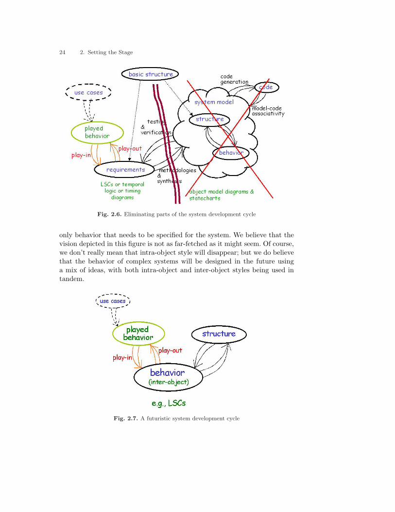
As discussed in the previous chapter, we believe that the LSC specifica-tion, together with the play-in/play-out approach, may be considered to benot just the system’s requirements but actually its final implementation. Amore modest goal would be to build system prototypes by first creating theapplication GUI and then playing in the behavior, instead of coding it. Thesame holds for constructing tutorials for system usage prior to actual systemdevelopment. Thus, we strongly believe there is a potential to use the Play-Engine and its underlying ideas not only for isolated parts of a developmentcycle, but throughout the entire cycle. Figure 2.6 shows the parts of the de-velopment cycle that could become eliminated for certain kinds of systems.
Figure 2.7 shows a futuristic development cycle, where the played-in be-havior is not considered merely as requirements, but is actually used as the
24 2. Setting the Stage
Fig. 2.6. Eliminating parts of the system development cycle
only behavior that needs to be specified for the system. We believe that thevision depicted in this figure is not as far-fetched as it might seem. Of course,we don’t really mean that intra-object style will disappear; but we do believethat the behavior of complex systems will be designed in the future usinga mix of ideas, with both intra-object and inter-object styles being used intandem.
Fig. 2.7. A futuristic system development cycle

3. An Example-Driven Overview
In this chapter, we overview the main ideas and principles of our work. Thepurpose of the overview is to give a broad, though very high-level, view of theLSC language, the play-in methodology for specifying inter-object scenario-based behavior, and the play-out mechanism for executing such behavior. Wewill touch upon many issues, but will not dwell on the details of the languageconstructs, nor the methodology, nor the tool. The overview is presented asa guided walk-through, using a simple example of a reactive system.
3.1 The Sample System
Consider a bakery, in which different kinds of bread, cakes and cookies arebaked in three ovens. Suppose Ms. B., the owner of the bakery, wants toautomate the bakery by adding a bakery panel that will control and monitorthe three ovens. According to the play-in approach, the first thing to do is toask our user, Ms. B, to describe the desired panel. In this preliminary phase, avery high-level description, focusing on the panel’s graphical user interface(GUI), is sufficient. The panel, coded using some rapid development language(or a special-purpose tool, as we discuss later) is shown in Fig. 3.1. The panel
Fig. 3.1. A central panel controlling the bakery’s ovens

26 3. An Example-Driven Overview
has a main switch and a main light in its top-left corner. On the top right,there is a console display, which is used to show textual messages. The restof the GUI contains three 3-state switches, three thermometers and threewarning lights. Each set of switch, thermometer and light is used to controland monitor a different oven.
Note that this bakery panel is nothing but a graphical user interface. Nobehavior is programmed into it, and all it can do is interact with the Play-Engine tool in a rather trivial way. All the behavioral requirements of thispanel will be defined as we go along. As we progress with the example, wemay add more graphical elements to the panel and define their behavior aswell.
3.2 Playing In
Having the GUI application at hand, Ms. B. is ready to specify the requiredbehavior of the bakery panel. She wants to add a new LSC and give it aname. Figure 3.2 shows the Play-Engine with the empty LSC just added.The top blue dashed hexagon is the LSC’s prechart and the bottom solidrectangle is its main chart. The prechart should contain a scenario, which,if satisfied, forces the satisfaction of the scenario given in the main chart.The relation between the prechart and the chart body can be viewed as anaction-reaction; if and when the scenario in the prechart occurs, the systemis obligated to satisfy the scenario in the main chart.
The first thing our user would like to specify is what happens when thebakery panel is turned on. Since this is done using a switch, the action ofclicking the switch is put in the prechart, and the appropriate system re-actions are put in the chart body. In our case, we want the system, as aresponse, to turn on the light and to change the display’s color to green.
The process of specifying this behavior is very simple. First, the user clicksthe switch on the GUI, thus changing its state1 from Off to On. When thePlay-Engine is notified of this event, it adds the appropriate message in the(initially empty) prechart of the LSC from the user instance to the mainswitch instance. See Fig. 3.3.
The user then moves the cursor (a dashed purple line) into the chart bodyand right-clicks the light on the GUI. The engine knows the properties of thelight (in this case, there is just one) and pops up a menu, from which the userchooses the State property and sets it to On. Figure 3.4 shows the popupmenu that is opened after the light is right-clicked, and the dialog that opens1 We use the word ‘state’ to describe a property of the switch. This should not to be
confused with the term ‘state’ from finite state machines and statecharts.

3.2 Playing In 27
Fig. 3.2. An empty universal LSC in the Play-Engine
after the State property is chosen. A similar process is then carried out forthe background property of the display. After each of these actions, the engineadds a self-message in the LSC from the instance representing the selectedobject, showing the change in the property. The Play-Engine also sends amessage to the GUI application, telling it to change the object’s property inthe GUI itself so that it reflects the correct value after the actions have beentaken. Thus, when this stage is finished, the GUI shows the switch on, thelight on, and the display colored green. Figure 3.5 shows the resulting LSCand the status of the GUI panel.
Suppose now that the user wishes to specify what happens when the switchis turned off. In this case we want the light to turn off and the display tochange its color to white and erase any displayed characters. The user may,of course, play in another scenario for this, but these two scenarios will bevery similar, and they are better represented in a single LSC. This can bedone using symbolic messages. We play a scenario as before, with the switchbeing clicked as part of the prechart, and the system’s reactions being playedin as the chart’s body. However, this time we do it with the symbolic flag on.

28 3. An Example-Driven Overview
Fig. 3.3. The results of clicking the main switch to On
Fig. 3.4. Changing the light state to On
When in symbolic mode, the values shown in the labels of messages are thenames of variables (or functions), rather than actual values. So the user willnow not say that the light should turn on or off as a result of the prechart,but that it should take on the same state as the switch did in the prechart.The Play-Engine provides a number of ways of doing this. A variable canbe selected from a table of predefined variables or, as shown in Fig. 3.6, we

3.2 Playing In 29
Fig. 3.5. LSC: Turning on the panel
can indicate that the value should be the same as in some message in theLSC. Here Xs is a variable. For the second option, the user simply clicks the
Fig. 3.6. Symbolic mode: the light takes on the same state as the switch

30 3. An Example-Driven Overview
desired message inside the LSC and its variable will be attached to the newmessage as well.
This takes care of turning the light on or off. We now want to deal withthe display’s color. In one case it should become green and in the other white.We use an if-then-else construct for this. The user clicks the If-Then buttonon the toolbar and in response a wizard and a condition form are opened.Many kinds of conditions can be specified directly via the GUI, except that, incontrast to simple GUI-based actions, here several kinds of relation operatorscan be used (e.g., <,≤, >, etc.). Figure 3.7 shows the system after the wizardopens and the user clicks the switch on the GUI. Note that in the condition
Fig. 3.7. Specifying if-then-else using a wizard
form, the value of the switch is specified, and the switch itself is highlightedin the GUI. Conditions may refer to properties of GUI objects, to values ofvariables, or may even contain free expressions that the user will be requestedto instantiate during play-out.
After the if-then condition is specified, the user continues playing in thebehavior of the If part in the usual way. When this is completed, he/she clicks

3.2 Playing In 31
the Specify the ELSE part on the wizard and plays in the behavior for theElse part. The resulting LSC is shown in Fig. 3.8.
Fig. 3.8. An if-then-else construct
We could have specified in the Else part that the display should alsobe cleared (e.g., by asking to show an empty string). However, in order tointroduce and exemplify stand-alone conditions we do it in a different way.We already saw that conditions may serve in if-then-else constructs, but theycan also serve as stand-alone guards, either hot or cold. If a cold conditionis true, the chart progresses to the location that immediately follows thecondition, whereas if it is false, the surrounding (sub)chart is exited. A hotcondition, on the other hand, must always be met, otherwise the requirementsare violated and the system aborts. We will use a cold condition to checkwhether the switch is Off. If this is the case, the display is cleared, otherwisethe chart is gracefully exited and the display’s text does not change. A stand-alone condition can be inserted into the chart at any moment by clicking anappropriate button on the toolbar. After the button is clicked, the samecondition dialog that was used in the if-then-else construct is opened.
An object can participate in a condition without being actually con-strained. This is usually done when we want the object’s progress to besynchronized with the condition’s evaluation, but to have no effect on itsvalue. Synchronizing an object with a condition (i.e., making the object anon-influential part of the condition) is done by right-clicking the object andchoosing Synchronize from the popup menu. In our example, we want theconsole object to be synchronized with the condition but to have no effecton its value. Figure 3.9 shows how this is done.

32 3. An Example-Driven Overview
Fig. 3.9. Specifying a stand-alone condition guard
A condition hexagon will be stretched along the LSC, reaching all theinstances to which it refers. To distinguish such instances from those that donot participate in the condition’s definition or are not to be synchronized withit, the engine draws small semicircular connectors at the intersection pointsof the condition with the participating instance line. Figure 3.10 shows thefinal LSC and the way conditions are rendered.
One aspect of the LSC language that contributes to its flexibility is the factthat behaviors can be given in separate charts, and these can each describea fragment of a more complex behavior. When these fragments become rele-vant during execution is a consequence of their precharts, and thus no explicitorder is imposed on the charts (in contrast to the mechanism for combiningcharts in high-level MSCs, for example). So, suppose that our user has justdecided that when the switch is turned on, the three warning lights shouldflicker (by changing colors from green to red and back) three times, termi-

3.2 Playing In 33
Fig. 3.10. A symbolic LSC for turning the panel on or off
nating in green. One way to capture that is to go back to the LSC shownbefore and add this ‘piece’ of behavior in its correct place (i.e., in the ‘then’part of the if-then-else construct). Alternatively, we can create another LSC,which is activated only when the switch is turned On.
To do this, the user clicks the switch on the GUI to On while the cursor isin the prechart, in the same way as described earlier. We now want to specifythe three-fold flickering itself. Of course, we could simply play in the sixcolor changes for every light. It is better, however, to use the loop constructof LSCs. As with the if-then-else construct, a loop is inserted by clicking abutton on the toolbar, which causes a wizard to open. Figure 3.11 shows thewizard and the LSC during the process of specifying a loop.
Fig. 3.11. Specifying loops in LSCs

34 3. An Example-Driven Overview
There are three types of loops in LSCs. This one is a fixed loop; it isannotated by a number or a variable name, and is performed a fixed numberof times.
After selecting the desired type of loop using the loop wizard, the usercontinues playing in the required behavior in the same way as before. Theloop is ended by clicking the End Loop button in the loop wizard. Figure3.12 shows the resulting LSC. Note the special use of a cold condition in
Fig. 3.12. An LSC with a fixed loop
the middle of the loop. A condition with the reserved word SYNC is alwaysevaluated to true. (Actually, the reserved word TRUE could have been usedinstead, but SYNC reflects better the underlying intuition.) Placing such acondition where it is, and synchronizing the three lights with it has the effectof synchronizing the lights and forbidding a light to change its color to greenbefore the others have changed their color to red.
Thinking a bit more about the bakery panel, Ms. B. now decides that shewould like to be able to probe the thermometers for their exact temperature.To do that, some additional graphical objects should be added to the panel.Figure 3.13 shows the modified panel. Two selectors and one Probe buttonhave been added. One selector is used to select a thermometer and the otherto select the units for displaying the temperature (i.e., Celsius or Fahrenheit).
We now specify the following requirement:

3.2 Playing In 35
Fig. 3.13. The modified bakery panel
When the Probe button is clicked, the console should display the tem-perature of the thermometer selected using the thermometer selector.The temperature should be displayed in Celsius or Fahrenheit degrees,according to the units in the units selector.
The prechart is quite simple, and contains a single message denoting theevent of the user clicking the Probe button. In the chart body, we first want tostore the temperature of the selected thermometer. We do this using three if-then constructs. The temperature is stored in a variable using an assignmentconstruct. Assignments are internal to a chart, and can be used to save valuesof the properties of objects, or of functions applied to variables holding suchvalues. The assigned-to variable stores the value for later use in the LSC. Theexpression on the right-hand side contains either a reference to a property ofsome object (this is the typical usage) or a function applied to some predefinedvariables. It is important to note that the assignment’s variable is local tothe containing chart and can be used in that chart only, as opposed to thesystem’s state variables, which may be used in several charts. Figure 3.14shows how an object property can be stored, by right-clicking the desiredobject, choosing Store and then the desired property name. It also shows theresulting assignment, drawn as a rectangle folded in its top-right corner. Sinceafter storing a value we might like to refer to it later, and for this a meaningfulname is helpful, the Play-Engine lets the user name the assigned variable; herewe use Tc (since the original temperature is given in Celsius). Figure 3.15shows an LSC in which the variable Tc stores the required temperature.
Next, the console should display Tc according to the selected units. IfCelsius is selected, then Tc should be displayed as is. If Fahrenheit is selected,the temperature should be converted. This is an example of the need to usedata manipulation algorithms and functions that are applied to specifiedvariables. Such functions cannot (and should not) be described using LSC-

36 3. An Example-Driven Overview
Fig. 3.14. Using assignments to store the temperature
style interactions between objects, but rather should be imported as externalartifacts that have to be worked into the requirements. The Play-Engineallows the specification of an event value as a function applied to variables.These functions are user-implemented and their declarations are obtainedfrom the GUI application. Figure 3.16 shows the final LSC. Using an if-then-else construct, which depends on the units selector value, the console displaysthe temperature in the correct units, using the function Cels2Fahr to convertCelsius to Fahrenheit.
The next requirement our user wishes to express is the following:
If the temperature in one of the ovens gets below 30 degrees Celsius,the console should display a “Cold Oven!” warning message.
The temperature is a property of a thermometer, which is not changed by theuser or by the system. It is actually changed by the environment. Often, areactive system works in the presence of other elements, apart from the userwho interacts with it. Such elements might include other machines, comput-ers, sensors, and even Mother Nature. The collection of all these elements

3.2 Playing In 37
Fig. 3.15. Storing the temperature of the selected thermometer
Fig. 3.16. Probing and displaying a thermometer temperature
is referred to as the system’s environment. When playing in the requiredbehavior of a reactive system, it is necessary to be able to express its interac-tion with this environment. The Play-Engine allows the user to specify how

38 3. An Example-Driven Overview
the environment reacts with the system in a way similar to the interactionwith the end-user.
Figure 3.17 shows an LSC that describes the above requirement for ther-mometer ]1. When the temperature of thermometer ]1 is changed (by the
Fig. 3.17. Interacting with the external environment
environment) to some value T , and T is less than 30 degrees Celsius, thenthe console displays the required warning message.
We could have created two more charts for the other two thermometers,yet there is a more elegant way to do this. Many systems feature multipleobjects that are instances of the same class. This is one of the central maximsof the object-oriented paradigm. For example, a communication system con-tains many phones, a railroad control system may have not only many trainsand terminals but also many distributed controllers, etc. We would like tobe able to specify behavioral requirements in a general way, on the level ofclasses and their parameterized instances, not necessarily restricting them toconcrete objects. In our example, since the three thermometers are actuallythree instances of the same thermometer class, we would like to take the LSCshown in Fig. 3.17 and generalize it so that it deals with all the thermometersin the system. We can do this using an extension we have defined for LSCs,involving classes and symbolic instances. A symbolic instance is associ-ated with a class rather than with an object, and may stand for any objectthat is an instance of the class. Figure 3.18 shows the generalized version ofthe LSC of Fig. 3.17. In our example, a CTherm class was created and allthe thermometers were defined as instances thereof. In Fig. 3.18, the instancerepresenting thermometer ]1 was turned into a symbolic instance, and thusnow represents any object that is an instance of class CTherm.
Symbolic instances constitute a rather complex topic, raising several in-teresting and non-trivial issues that we deal with later in the book.

3.3 Playing Out 39
Fig. 3.18. Using symbolic instances to represent classes
3.3 Playing Out
After playing in the required behavior so far, Ms. B. is ready to check hermodel, and she therefore moves to play-out mode. Playing out is the processof testing the behavior of the system by providing any user actions, in anyorder, and checking the system’s ongoing responses. The play-out processcalls for the Play-Engine to monitor the applicable precharts of all universalcharts, and if successfully completed to then execute their bodies. As dis-cussed earlier, the universal charts contain the system’s required reactions toother actions. By executing the events in these charts and causing the GUIapplication to reflect the effect of these events on the system objects, the useris provided with a simulation of an executable application.
Note that in order to play out scenarios, the user does not need to knowmuch about LSCs or even about the use cases and requirements entered sofar. All he/she has to do is to operate the GUI application as if it were a finalsystem and check whether it reacts according to the expectations.
We should emphasize that the possible runs of the system are not sim-ply different orders of the same sequences of inputs, but can include totallydifferent runs that contain unexpected events and messages. This is doublytrue in the presence of symbolic instances, symbolic messages and unboundedloops.
The underlying play-out mechanism can be likened to an over-obedientcitizen who walks around with the Grand Book of Rules on him at all times.2
He doesn’t lift a finger unless some rule in the book says he has to, never doesanything if it violates some other rule, and always carries out — to the letter— what he was asked to do, as well as anything else that doing so entails.He constantly scans and monitors all rules at all times. Clearly, in so acting,2 Chapter 5 contains this idea applied to a female citizen too.
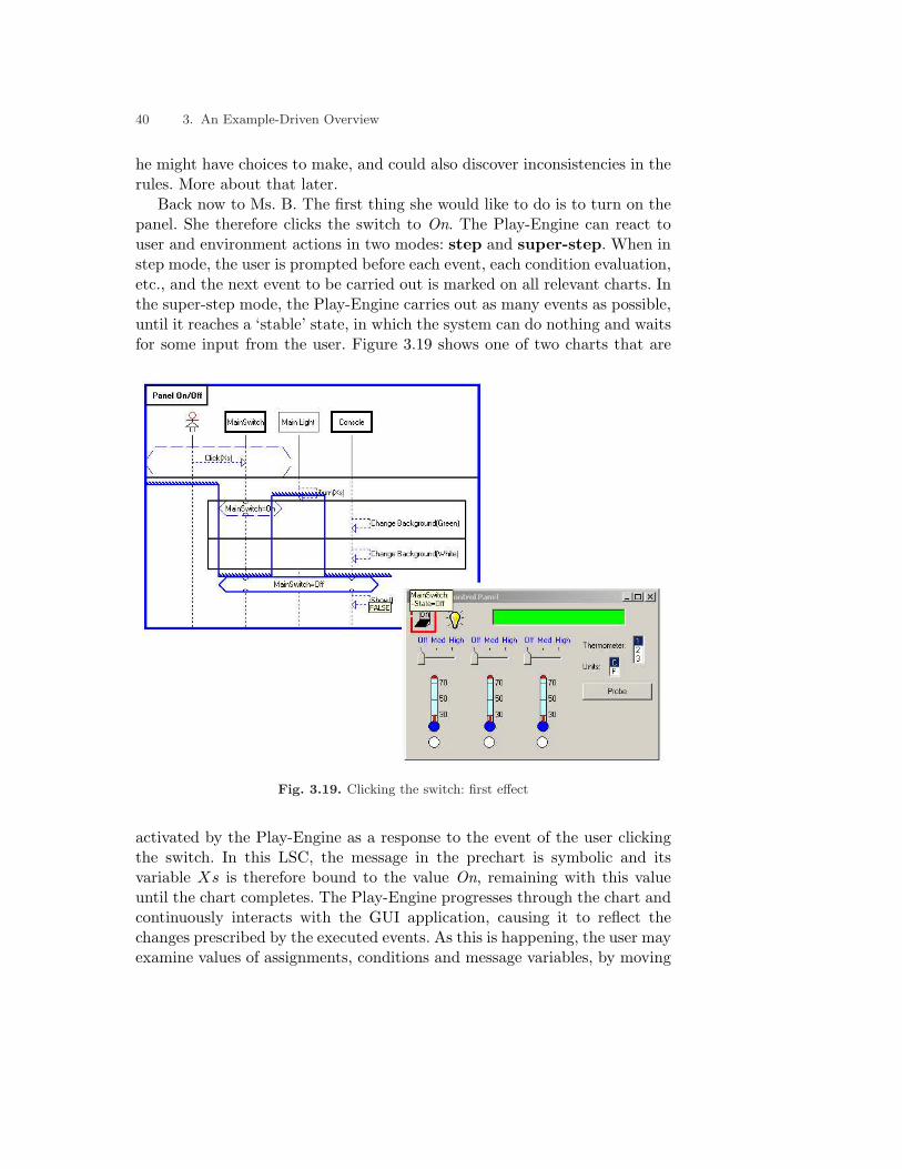
40 3. An Example-Driven Overview
he might have choices to make, and could also discover inconsistencies in therules. More about that later.
Back now to Ms. B. The first thing she would like to do is to turn on thepanel. She therefore clicks the switch to On. The Play-Engine can react touser and environment actions in two modes: step and super-step. When instep mode, the user is prompted before each event, each condition evaluation,etc., and the next event to be carried out is marked on all relevant charts. Inthe super-step mode, the Play-Engine carries out as many events as possible,until it reaches a ‘stable’ state, in which the system can do nothing and waitsfor some input from the user. Figure 3.19 shows one of two charts that are
Fig. 3.19. Clicking the switch: first effect
activated by the Play-Engine as a response to the event of the user clickingthe switch. In this LSC, the message in the prechart is symbolic and itsvariable Xs is therefore bound to the value On, remaining with this valueuntil the chart completes. The Play-Engine progresses through the chart andcontinuously interacts with the GUI application, causing it to reflect thechanges prescribed by the executed events. As this is happening, the user mayexamine values of assignments, conditions and message variables, by moving

3.3 Playing Out 41
the mouse over them in the chart. In this example, the mouse is located overthe cold condition. As a result, the condition is evaluated and a tooltip showsthe valuation result (false). At the same time, the GUI objects participatingin the condition are highlighted in the panel and each one displays a tooltipwith its relevant constraints. Since this cold condition evaluates to false, thechart completes (denoted by the surrounding blue thick frame).
Figure 3.20 shows the second chart that is activated as a result of clickingthe switch to On. In this figure, the Play-Engine is in step mode, after some
Fig. 3.20. Clicking the switch: second effect
steps have already been taken. The next step to be taken is circled in red.The number in the top-right corner of the loop shows how many iterationshave already been performed; the numbers in the top-left corner denote thecurrent and total iteration numbers. Note that in the bakery panel the firstwarning light has already changed to green while the other two are still red.

42 3. An Example-Driven Overview
After turning on the panel, our user, Ms. B., wishes to test the effect ofone thermometer going below 30 degrees Celsius. To do that, she has to playthe role of the environment. Figure 3.21 shows how this is done. The user
Fig. 3.21. Playing out the environment
right-clicks the desired object (in this case thermometer ]2), selects ExternalChange and then chooses the property to be changed. Here, Ms. B. choosesTemp and then enters a value of 20 degrees (not shown in the figure). As aresult, the chart in Fig. 3.22 is activated and is completed. Recall that the
Fig. 3.22. Play-out: binding symbolic instances
scenario in this chart was played in using thermometer ]1, and the instancerepresenting it was turned symbolic. Now, since Ms. B. played out usingthermometer ]2, the symbolic instance is bound to this thermometer for therest of the scenario.
Thus, as explained earlier, playing out enables the user to actually activatethe specified system directly from the scenario-based inter-object behavioral

3.4 Using Play-Out for Testing 43
specification — possible and mandatory scenarios, forbidden scenarios andother constraints — without the need to prepare statecharts, to write orgenerate code, or to carry out any other detailed intra-object thinking. Theprocess is simple enough for many kinds of end-users and domain experts,and can greatly increase the chance of finding errors early on.
3.4 Using Play-Out for Testing
Universal charts ‘drive’ the model by their action-reaction nature, whereasexistential charts can be used as system tests or as examples of requiredinteractions. Rather than serving to drive the play-out, existential charts aremonitored; that is, the Play-Engine simply tracks the events in the chartas they occur. When (and if) a traced chart reaches its end, it is highlighted,and the user is informed that it was successfully traced to completion. Theuser may select the charts to be monitored, thus saving the Play-Engine theneed to track charts that might currently not be of interest.
Figure 3.23 shows an existential chart that was successfully traced tocompletion. This chart represents a test (as indicated by the “T” in the top-left corner), stating that after the switch is turned on, the light should be
Fig. 3.23. Monitoring existential charts

44 3. An Example-Driven Overview
on and the console and the three warning lights should all be green. As atest, this LSC is not required to explicitly show how the required result isaccomplished but only that it is eventually accomplished. The required testresults are specified using a hot condition, thus enabling the chart to completeonly if the condition evaluates to true.
When playing out the GUI application, a run trace is produced, whichincludes all the user actions and the system reactions. These runs can berecorded, to provide testimonies (that can be replayed) for fulfilling existentialLSCs. Recorded runs can be saved (in XML format) and then reloaded. Moreimportantly, runs can be imported from different sources and then be replayedin the same manner. These external sources can be different implementationsof the specification, either given as executable programs or as more detaileddesign models, (e.g., statecharts, labeled transition systems, etc.). Importinga run from an implementation and replaying it, while tracing all charts, canbe used to show that the implementation is consistent with the requirementsin the sense that existential charts are successfully traced and universal chartsare not violated.
3.5 Transition to Design
After playing in the requirements using the GUI application, and validatingthem using play-out, the Play-Engine can be used to make a smooth transi-tion into the design phase. In many development methodologies, the designerbegins the design phase with a requirements specification, usually given asa text document, and then constructs scenarios (say, in some variant of se-quence diagrams) to show the interaction between the objects comprisingthe system, and to become convinced that these scenarios satisfy the originalrequirements.
Using the play-in methodology, the designer can begin the design phasewith a set of given (and debugged) LSCs that describe the requirementsin terms of allowed and forbidden interactions between the system and itsusers and environment. The design phase would then consist of going throughthe universal charts and refining them by adding internal objects and theinteractions between these objects and the GUI objects and other internalobjects. Adding this information to the charts fills the gap between what thesystem should do and how it does it. Note that by starting with LSCs createdby, or on behalf of, the user, we achieve near-perfect traceability betweenthe requirements and the design. Moreover, by leaving the existential chartsunmodified, the designer may prove the correctness of the modified LSCs byperforming regression testing to satisfy the original existential charts.

3.5 Transition to Design 45
The Play-Engine provides means for adding internal objects on the fly. Italso enables the addition of properties and methods to the new objects andalso to the objects exported by the GUI application. The internal objects aredrawn in an object map, which is a kind of object model diagram. In thisdiagram, each object is shown with all its methods, its properties and theirvalues.
Suppose that in our bakery panel example the designer wants to specifyhow the light is turned on or off after the switch is clicked. He/she decidesthat a new switch controller, Sw-Ctrl, will be used. Figure 3.24 shows anobject map with the new object and an LSC that shows how the informationis transferred from the switch to the light.
Fig. 3.24. Playing out internal objects
When LSCs containing method calls are played out, the Play-Engine ani-mates them by drawing arrows between the involved objects and highlightingthem. Thus, the play-out mechanism can be used not only to help end-usersvalidate requirements but also as a useful tool for demonstrating, reviewingand debugging a design. Figure 3.24 shows how interaction between objectsis animated in the Play-Engine. Note that the arrows are not limited to beinginternal to the GUI application or to the object map themselves, but can runfrom one to the other.

46 3. An Example-Driven Overview
3.6 Time
Many kinds of reactive systems must explicitly refer to and react to time.Suppose that Ms. B. is not satisfied with the standard way the lights havebeen made to flicker as the panel is turned on (Fig. 3.25(a)), but wants themto remain red for one second and green for two seconds.
We have extended the LSCs to handle time by adding a single clock objectwith one property, time, and one method,Tick.
Using the clock object together with the existing constructs of LSCs, wecan specify a wide variety of timing constraints and time-driven events. Figure3.25(b) shows an LSC that describes the modified requirement. Before thelights change to red, the time is stored in a variable T . Before they change togreen, the hot condition Time > T must first be satisfied, and this happensonly after the elapse of one second. The same goes for the change from greento red, except that in this case the condition forces a delay of two seconds.
Reactive real-time systems are often required to react to the passage oftime and not only to refer to it when constraining the intervals betweenactual events. Suppose that in our case Ms. B. wishes to continuously probethe selected thermometer at a rate of one probe per second. For this we adda new internal object, Prb-Ctrl, which will be responsible for the probingprocess. This probe-controller object has one Boolean property, IsProbing,that shows whether the object is probing, and two methods, ToggleProbe tostart and stop the probing process and ProbeOnce to activate a single probe.Figure 3.26 shows the object map with the new object and an LSC thatdescribes how Prb-Ctrl is stimulated by the Probe button.
Figure 3.27(a) shows how the clock ticks can be referred to in LSCs. TheLSC in this figure specifies that if the probe controller is probing and a clocktick occurs, then the probe controller calls itself to perform a single probe.Figure 3.27(b) shows that when Prb-Ctrl calls its Probe method, it performsa single probe as described earlier. Hence, when the probe controller is inprobing mode, each clock tick activates the ‘Probe Tick’ LSC, and this inturn activates the ‘One Probe’ LSC in a chain reaction.
The play-out mechanism supports LSCs that refer to time. Specificationscan be executed in manual clock mode, where the user advances the clockby clicking a Tick button, or in automatic clock mode, where the clockticks are performed by the Play-Engine at fixed intervals (which can be de-termined by the user).

3.7 Smart Play-Out 47
Fig. 3.25. Specifying time constraints
3.7 Smart Play-Out
As described earlier, play-out is actually an iterative process, where aftereach step taken by the user, the Play-Engine computes a super-step, whichis a sequence of events carried out by the system as the response to the event

48 3. An Example-Driven Overview
Fig. 3.26. Toggling the probe controller using the Probe button
input by the user. However, the ‘obedient citizen’ mechanism of the play-out process is rather naive, for several reasons. For example, there can bemany sequences of events possible as a response to a user event, and someof these may not constitute a ‘correct’ super-step. We consider a super-stepto be correct if when it is executed no active universal chart is violated. Byacting blindly according to the ‘Grand Book’ of requirements, reacting to auser-generated event with the first action it finds that is a possible reactionto that event, the naive play-out process could very well follow a sequenceof events that eventually causes violation, whereas another sequence couldhave been chosen that would have completed successfully. The multiplicityof possible sequences of reactions to a user event is due to the fact that adeclarative, inter-object behavior language, such as LSCs, enables the formu-lation of high-level requirements in pieces (e.g., scenario fragments), leavingopen details that may depend on the implementation. The partial order se-mantics among events in each chart, and the ability to separate scenarios indifferent charts without saying explicitly how they should be composed arevery useful in early requirement stages, but can cause underspecification andnondeterminism when one attempts to execute them.
Consider, for example, the two charts given in Fig. 3.28. ‘LSC1’ says thatwhen the main switch is turned on, the first warning light turns green, thefirst switch is automatically set to Med and the console displays the stringSwitch1 Med. Note that the LSC does not enforce any particular order onthese three events, so that there are several possibilities for the order inwhich they execute, and the play-out mechanism will choose one, in a waythat is not controllable by the user.

3.7 Smart Play-Out 49
Fig. 3.27. Periodic probing
‘LSC2’ says that whenever the state of the first switch is set to Med, thefirst light should not yet be green. Then this light turns green, and only thendoes the console display the string Switch1 Med.
If these are the only two specified charts, and the user turns the switchto On during play-out, the play-out mechanism chooses the events in anorder that results in the charts shown in Fig. 3.29. The first event to betaken is the top-most, i.e., changing the color of the first light to green. Thesecond is setting the state of Switch1 to Med. As this event occurs, ‘LSC2’is activated but cannot progress, since the warning light is green. ‘LSC1’

50 3. An Example-Driven Overview
Fig. 3.28. Nondeterministic choice during play-out
is also not allowed to progress, since the event of showing Switch1 Med onthe console violates ‘LSC2’. Therefore, no progress is allowed at all and thesuper-step terminates.
The smart play-out approach focuses on executing the behavioral re-quirements with the aid of formal analysis methods, mainly model-checking.The smart play-out process finds a ‘correct’ super-step if one exists, or provesthat such a super-step does not exist. This is achieved using model-checkingat the occurrence of each user event, in order to examine the different poten-tial super-steps and to find a correct sequence of system reactions if there isone. Model-checking thus drives the execution. Another way of putting it isthat the ‘smartness’ in smart play-out works as an aid, helping the objectsin the system cooperate in fulfilling the requirements.
In our example, the result of applying the smart play-out algorithm forfinding the correct super-step is shown in Fig. 3.30. In this case, the firstevent taken after the main switch is turned on is that of changing the stateof Switch1 to Med. This event activates ‘LSC2’, but this time the warninglight is not green yet. The hot condition is thus evaluated to true and is

3.7 Smart Play-Out 51
Fig. 3.29. Standard play-out
propagated. Now the event of changing the warning light to green can becarried out, affecting both charts. Next the cold condition is successfullypassed, and again the event of showing Switch1 Med on the console can beperformed, causing the successful completion of both charts.
Smart play-out illustrates the power of putting formal verification meth-ods to use in early stages of the development process, with the potential ofimpacting the development of reactive systems. More ways of utilizing smartplay-out in the Play-Engine and the details of the smart play-out algorithmsare discussed in Chap. 18.

Fig. 3.30. Using smart play-out

Part II
Foundations


4. The Model: Object Systems
Scenario-based languages, such as LSCs, are not restricted to particular sys-tems, architectures or modeling techniques. They can serve to specify thebehavior of either sequential or parallel systems, based on either centralizedor distributed architectures, and they can be used to describe the interactionbetween processes, tasks, functions and objects. The same applies to virtu-ally all the ideas and techniques described in this book. However, it will beconvenient for us to use a single system model throughout the book. Sinceobject-orientation appears to be the most dominant development methodol-ogy today, we will use the basic OO notions and terminology in our systemmodel as well.
To describe the structure of a reactive system within the play-in/play-outmethodology and the supporting Play-Engine tool, we use object systems.In our setting, a system consists of an arbitrary number of objects, eachof which embodies an arbitrary number of properties. Since the approach isnot restricted to modeling applications and systems from a specific domainor field, the object’s properties are based upon application types, which arealso considered part of the system model. Each object may be an instanceof some defined class. An object that is not explicitly associated with a classis considered to be the single object in a special singleton class having thesame properties as the object itself.
In this chapter, we describe the various elements comprising a systemmodel. As we continue our description of the more advanced elements andfeatures of the language and the play-in/play-out approach, the system modelwill be extended appropriately.
4.1 Application Types
The most basic element in our models is an application type. When clearfrom the context, we will refer to application types simply as types. Thereare three kinds of types:
Enumeration type – defined by a finite set of values.

56 4. The Model: Object Systems
Discrete type – defined by a minimum value, a maximum value and a step(delta) that defines the interval between two consecutive values. For ex-ample, a discrete type having 0, 10 and 1 as its minimum, maximum anddelta, respectively, contains the integers between 0 and 10, inclusive.
String type – defined by a maximal length.
Each type is identified by a name and a unique ID, and may be providedwith a description. Here are some examples of application types.
Color – The possible colors that can be used in an application can be de-scribed using an enumeration type that consists of the different colornames (e.g., {Red, Blue, Green, White, Black, ...}). To represent a 24-bitcolor we could use a discrete type with integer numbers ranging from0 to 224 − 1, with a delta of 1, thus representing all the possible RGBcombinations.
Boolean – The Boolean type is defined simply as an enumeration containingthe values {True, False}.
Character – Characters can be defined using a string type of length 1. Analternative way would be to use a discrete type, with the characters en-coded by their ASCII codes.
Byte – A byte can be represented by a discrete type ranging from 0 to 127with a delta of 1, or by a string type of length 8, which would explicitlyshow the bits constituting the byte.
The choice of the type for a particular application should be made so thatits representation is the most convenient for the way it will be used.
4.2 Object Properties
Every object in the application is associated with a set of properties. Thevalues of the properties for GUI objects are usually reflected in the waythese objects are rendered in the application, but this is not mandatory.1
A property has a name and is identified by a unique ID (unique within theobject scope). Each property is based on a type, from which its values can beselected.
In order to provide an intuitive and user-friendly support for play-in andplay-out, we require object properties to also have the following characteris-tics:
Prefix – The property prefix is a verb used to describe the action of changingthe property’s value (e.g., show a value, turn the light on/off, etc.). Thisfeature is used mainly to help make the specification clear and intuitive.
1 In Chap. 14 we discuss how GUI-less objects display their property values.

4.2 Object Properties 57
Is default – If a property is default, its name is not shown in the LSC mes-sages. Let us take for example, a light object with one property, State,that can be on or off. If the property is not declared as default, thenwhen the light is turned on the message in the chart will read “TurnState(On)”, whereas if it is declared as default the message will read“Turn(On)”. Again, this feature is used to make the requirements clearerby hiding redundant information in the charts.
In only – Object properties are usually changed by either operating the ob-ject (e.g., clicking a switch, moving a slider, etc.), or by right-clickingit and then choosing a property from a popup menu and specifying itsnew value. The first method is used to demonstrate user actions whilethe second is used to specify system reactions. An in only property canbe changed only using the first of these, and therefore is not shown onthe object’s right-clicked popup menu (e.g., a button in a GUI is usu-ally clicked by the user, hence there is no reason why one would want tospecify that the button was clicked by the system).
Can be changed externally – This indicates that the property can be changedby the system’s environment (i.e., some external element other than theend-user). When playing in behavior, changes caused by the environmentare played by right-clicking an object, choosing “External Change” andthen selecting the property to be changed. Only properties that can bechanged externally are shown on that menu.
Affects – When the value of an object’s property is changed, a message isdrawn in the LSC. The value of the Affects flag shows how this arrow isdrawn; the possibilities are User, Env and Self, and the arrow is drawntowards the user, towards the environment, or as a self arrow, respectively.
Synchronous – A message referring to a synchronous property may be prop-agated only if both the sender of the message and its receiver are ready.The arrowhead of a synchronous message is different too.
Examples of object properties are the state of a light or a switch, the valueshown in a display, the background color of a display, and the temperatureshown on a thermometer.
The current implementation of our Play-Engine calls for a GUI applicationto be described as an XML application description file. Appendix B gives thedetailed structure of such files. This method of describing the system modelis merely an implementation issue, and it can be carried out in various otherways.

58 4. The Model: Object Systems
4.3 And a Bit More Formally ...
An object system Sys is defined as
Sys = 〈D, C,O〉
where D is the set of application types (domains), C is the set of classes andO is the set of objects. We refer to the user of the system as User and to theexternal environment as Env.
A class C is defined as
C = 〈Name,P〉
where Name is the class name and P is the set of class properties. An objectO is an instance of some class and is therefore defined as
O = 〈Name, C,PV〉
where Name is the object’s name, C is its class and PV : C.P → ⋃i Di is a
function assigning a value to each of the object’s properties. We define thefunction class : O → C to map each object to the class it is an instance of.We will also use the shortcut V alue(O.P ) = O.PV(O.C.P ) to denote thecurrent value of property P of object O.
An object property P is defined as
P = 〈Name,D , InOnly ,ExtChg ,Affects,Sync〉
where Name is the property name and D is the type it is based on. In-Only, ExtChg and Sync range over {true, false}, and Affects ranges over{User,Env,Self}, as explained earlier. The IsDefault and Prefix characteris-tics are purely cosmetic and do not affect the semantics of the model. We donot formalize the different kinds of application types, but rather view a typeD as a finite set of values.

5. The Language: Live Sequence Charts (LSCs)
Message sequence charts (MSCs) were discussed in Chap. 2. They wereadopted long ago by the International Telecommunication Union (the ITU,formerly the CCITT), and constitute a visual scenario-based language thatis popular in the realm of object-oriented systems for capturing behavioralrequirements. The language also manifests itself in the UML, somewhat mod-ified, and is referred to there as sequence diagrams.
Objects in MSCs are represented by vertical lines, called instances,1 andmessages going between these instances are represented by horizontal (orsometimes down-slanted) arrows. Every instance line contains locations. Aninstance progresses from one location to the next by participating in someactivity associated with the location. Such an activity could, for example,be the sending or receiving of a message. Every instance has also an initiallocation and a final location, in which the instance begins and terminates,respectively.
As explained in Chap. 2, the semantics of all known versions of MSCs,including the ITU standard and the UML sequence diagrams, is a set ofsimple constraints on the partial order of possible events in some possiblesystem execution, i.e., a partial order among the instance locations. Thispartial order is determined by two simple rules. First, time is assumed to gofrom top to bottom, so the partial order restricts the locations along a singleinstance to be processed in that order. Second, for asynchronous messages(most uses of MSCs are restricted to such messages), the send event of themessage precedes the receive event. For synchronous messages the two eventsare simultaneous. The partial order is essentially the transitive closure ofthese two rules. For a given chart L, we refer to the partial order it inducesby ≤L. Virtually nothing can be said in MSCs about what the system willactually do when run. The charts can state what might possibly occur, butnot what must occur, and neither can MSCs specify anti-scenarios, whoseoccurrence we want to forbid.1 The term instance is given in the MSC standard to describe the vertical line representing
an object, a process or a task. It should not be confused with class instances, a termused in object-oriented methods.

60 5. The Language: Live Sequence Charts (LSCs)
5.1 Constant LSCs
We now describe the basic version of live sequence charts (LSCs), pro-posed in 1998 by W. Damm and the first-listed author of this book. Theyeliminate the above deficiencies by their ability to specify liveness, i.e., thingsthat must occur. This is done by allowing the distinction between possibleand necessary behavior both globally, on the level of an entire chart, andlocally, when specifying events, conditions and progress over time within achart.2
LSCs have two types of charts: universal (annotated with a solid border-line) and existential (annotated with a dashed borderline). Universal chartsare used to specify restrictions that apply to all possible system runs. Eachuniversal chart is associated with a prechart that specifies the scenario that,if successfully executed, forces the system to satisfy the scenario given in theactual chart body. Existential charts are more like MSCs and UML sequencediagrams. They are used in LSCs to specify sample interactions between thesystem and its environment and must be satisfied by at least one system run.They thus do not force the application to behave in a certain way in all cases,but rather state that there is at least one set of circumstances under whicha certain behavior occurs. Existential charts can be used to specify systemtests, or simply to illustrate longer (non-restricting) scenarios that provide abroader picture of the behavioral possibilities to which the system gives rise.We will see more on this later, particularly in Chaps. 12 and 18.
Figure 5.1 shows a universal chart and an existential chart. Although the
Fig. 5.1. Universal and existential charts
2 Recently, there has been an attempt to adopt some of the ideas of LSCs in an extensionof UML sequence diagrams, which will feature certain constructs that specify mandatorybehavior. We are not familiar with the details of this extension, nor with the level ofrigor of its semantics, but some variant of the extension will probably become part ofthe UML 2.0 standard.

5.1 Constant LSCs 61
two contain the same events, their semantics are very different. The universalchart (Fig. 5.1(a)) says that every time the user clicks the switch to on, thelight should turn on. Hence, a universal chart induces an action-reactionrelationship between the scenarios in its prechart and the scenarios in thechart body, and these action-reaction pairs must be satisfied during the entiresystem run. The existential chart merely says that there is at least one run ofthe system, and one point during that run, in which the user clicks the switchto on and the light indeed turns on. It is important to note that there is nocausality between the two events in the existential chart. Actually, in thischart the events are not even restricted by the partial order, and therefore ascenario in which the light turns on and then the user clicks the switch to onalso satisfies the chart.
The small circles shown in the charts are the instance locations. All in-stances have at least three locations: an initial location, a location associatedwith the beginning of the main chart, and a final location. In the universalchart, all the instances that participate in the prechart have also a locationfor the prechart start. The beginnings of the prechart and the main chartare synchronization points; all instances enter the prechart simultaneously,while the main chart may be entered only after all instances have successfullycompleted their activities in the prechart.
A location may be either hot, thus forcing the instance to progress, orcold, thus enabling the instance to remain in its location without violatingthe chart. A hot location is denoted by a red circle and a solid line from thelocation to its successor. A cold location is denoted by a blue circle and adashed line.
As we shall see later, locations may be attached to various kinds of events,but in this chapter we restrict our discussion to LSCs that contain only themost basic events — sending and receiving constant messages.
Messages in LSCs may also be hot or cold. A hot message must bereceived after it is sent. A cold message may be sent and not received (whichcan be viewed as expressing a communication failure). Hot messages aredenoted by red solid lines and cold messages are denoted by blue dashedlines.
Messages can represent synchronous or asynchronous interactions. Selfmessages are always synchronous, so properties that have their Affects at-tribute set to Self are always represented by synchronous messages. Sincethe user and the environment are external to the system and therefore in-teract with the GUI objects directly, and not by sending messages over acommunication channel, most properties are defined as synchronous. Whenit is important to show that the interaction of the user or the environmentwith an object may take time from the moment the action is performed until

62 5. The Language: Live Sequence Charts (LSCs)
the object notices it, asynchronous properties can be used. We use closedtriangular arrowheads to denote synchronous messages, see Fig. 5.2(a), andopen arrowheads for asynchronous ones, see Fig. 5.2(b).
Fig. 5.2. Synchronous vs. asynchronous messages
5.2 Playing In
Messages in LSCs are used to indicate different kinds of events and interac-tions in the system. Here, we further restrict our discussion to messages thatreflect changes in property values only. Other kinds of messages are discussedin Chap. 14.
As an example system we use the bakery panel described in Chap. 3.Suppose we wish to specify that every time the main switch is clicked to On,the main light should turn On. The LSC in Fig. 5.3 describes this requirement.The text in the small box on the right is a natural language description,generated automatically from the LSC by the Play-Engine.
Fig. 5.3. Turning the bakery panel on

5.2 Playing In 63
In this example, the value of the switch’s state property is changed to Onby the user simply clicking it as is done with a working system. In response,the state property of the light is also changed to On, this time by the system(i.e., the object itself). Note that the locations along the light’s instance lineare hot (denoted by solid line segments), thus forcing the light to be turnedon if the prechart is successfully completed. Each of the two messages in thechart is a constant message (sometimes referred to as an exact message). Aconstant message is parameterless, i.e., is one for which all the informationit represents — the identities of the sender and receiver and the messagecontent — is known and fixed.
The value of an object’s property can be changed by the end-user of thesystem (e.g., by clicking a switch, rotating a knob, typing text in a text box,etc.). When specifying behavioral requirements, these kinds of events areplayed in using the same actions, i.e., operating the GUI objects as is donein the final system.
Typically, the system responses are also reflected by changes in the valuesof object properties (e.g., a light turns on, a console displays some text, etc.).Since these kinds of objects and properties cannot be directly operated by theuser to specify the desired value, the changes are specified by right-clickingthe target object. The Play-Engine then shows a popup menu, which showsall the properties of the selected object according to the system model (seeFig. 5.4(a)). After selecting a property from the menu (in this example, the
Fig. 5.4. Specifying the system’s response
light has only one property — state), a dialog opens where the user canspecify the new value. If the property is based on an enumeration type, thelist of values is shown and the user may select a value from there (see Fig.5.4(b)).

64 5. The Language: Live Sequence Charts (LSCs)
A property value of an object can be changed not only by the end-user orby the system but also by the system’s external environment. In the bakerypanel example, one may wish to specify that when the temperature of ther-mometer ]1 reaches 100 degrees, the system should react in some specifiedway. A thermometer is a sensor that indicates the value of some property(temperature), which is controlled neither by the user nor by the system.Therefore, there should be a way to express changes in this property causedby the external environment. Figure 5.5 illustrates how this is done and showsthe resulting message. In order to specify a change in one of the properties
Fig. 5.5. Referring to the environment
of an object, caused by the environment, the object is right-clicked, and theuser chooses External Change. Then, from the sub-menu, he/she choosesthe property to be changed (in this example Temp), and the property’s valueis inserted in the same way as for other changes. The Play-Engine then in-serts into the LSC a special instance representing the environment, and anappropriate message going from it to the target object.
When a property is changed by the user or the environment, the messageindicating the change goes from the user or the environment instances to theinstance representing the affected object. When specifying a system response,the resulting message originates from the changing object and arrives atone of three possible instances, determined by the Affects attribute of thechanged property, which ranges over {User, Self, Env}. Typically, propertieshave their Affects property set to Self, since it is common to view a changein the state of an object as a local event involving no other object or entity.

5.3 The General Play-Out Scheme 65
However, when we wish to emphasize that the change in the property is tobe seen by the user or the environment, the other options are used. Note,however, that the choice of the instance receiving the message may affect thepartial order induced by the LSC.
5.3 The General Play-Out Scheme
Like MSCs and UML sequence diagrams, LSCs can be used to specify re-quirements that serve later in the process of testing and validating moredetailed executable models or implementations. The set of events producedby a monitored system consists of property changes triggered by the userand the environment, as well as property changes triggered by the system’sobjects. A system event is identified by a message and an indication as towhether the message is being sent or received. The message contains the in-formation regarding the originator, the target object, the changed propertyand the new value for that property. When a run is being traced, the eventsfrom the run are continuously checked against the events in the LSCs toverify that the order induced by the LSCs in the specification is not violated.
This usage of LSCs is beneficial, and the language’s added expressivepower makes it possible to test and validate more powerful requirements.However, while the precursors of LSCs — MSCs and UML sequence diagrams— are used essentially only in this capacity, the expressive power of LSCsopens up a new and powerful possibility: executing them directly, withoutthe need for an intra-object model or implementation. This idea is one of themain issues this book attempts to cover in detail.
Behavioral requirements for a reactive system specify constraints on howthe system reacts with respect to external stimuli such as user actions, eventscoming from the external environment, timing events, etc. By way of execut-ing such behavior, we would like to enable the user to specify end-user orenvironment actions and for him/her to then be able to observe the systemresponses to these stimuli.
One must realize, however, that it is much harder to execute the behaviorgiven in an inter-object language, such as sequence diagrams or LSCs, thanit is to do so for intra-object languages such as statecharts, or for code. Thelatter provide clear information on each object’s reactions to every possibleevent. Thus, executing a system whose objects are described in an intra-object fashion is easy (at least in principle). In contrast, inter-object scenario-based languages do not contain explicit instructions for the behavior of eachobject under any given set of circumstances. If we want to be able to executebehavior given in such a language, the instructions for each object must be

66 5. The Language: Live Sequence Charts (LSCs)
figured out in runtime by considering all the relevant scenarios combined.This is the central issue that our execution mechanism has to address.
Before describing in detail how this is done, it is worth repeating verbatim(except for a gender change) the informal explanation given in the overviewchapter, Chap. 3: The underlying play-out mechanism can be likened to anover-obedient citizen who walks around with the Grand Book of Rules on herat all times. She doesn’t lift a finger unless some rule in the book says shehas to, never does anything if it violates some other rule, and always carriesout — to the letter — what she was asked to do, as well as anything else thatdoing so entails. She constantly scans and monitors all rules at all times.
More technically, our approach for executing LSCs can be described usingthe following general set of capabilities that an execution mechanism forinter-object behavior should supply:
1. Identify an external stimulus and find all the requirements that shouldbe considered when resolving the system’s response to it (e.g., identifythe event of flipping a switch and find all the requirements that specifythe system’s responses to the switch being flipped).
2. Apply the relevant requirements to create the sequence of system reac-tions. This is done iteratively, and thus includes identifying additionalrequirements that become relevant as the system is responding and ap-plying them too (e.g., after the switch is flipped, send a signal to thecontroller, which, in turn, may result in sending a signal to the light andturning it on).
3. Identify scenarios that are forbidden according to the requirements, andavoid generating them (e.g., make sure that if the requirements say thata certain signal cannot be sent to the light while it is on, it will indeednot be sent when the light is on).
4. In case a forbidden scenario actually occurs (e.g., because some othermandatory scenario forces it to, or as a result of a user action or anexternal action), indicate a violation.
Playing out is the process of testing the behavior of the system by provid-ing any user or environment actions, in any order, and checking the system’songoing responses. The play-out process calls for the Play-Engine to monitorthe applicable precharts of all universal charts, and if successfully completedto then execute their bodies. By executing the events in these charts and caus-ing the GUI application to reflect the effect of these events on the systemobjects, the user is provided with a simulation of an executable application.
When a universal LSC is activated, it can be in one of two activationmodes. As long as execution is in the prechart, the mode is said to bepreactive, and as soon as the prechart successfully completes, the mode

5.3 The General Play-Out Scheme 67
changes to active. After an LSC becomes activated, in either mode, each of itsinstances begins at its initial location and progresses as the run continues. Themapping of each instance of an LSC L to its current location is called a cutof L. A cut is hot if at least one of the instances is in a hot location and coldif all the instances are in cold locations. Cuts are drawn in the diagrams asthick comb-like lines (see Fig. 5.6). Note that in executing LSCs (and also inusing them for testing), a single universal chart may become activated severaltimes during a system run. Thus, we have to cater for multiple incarnationsof LSCs.
Fig. 5.6. An LSC cut
A run is consistent with an LSC if the events in the run occur in theorder dictated by the LSC. When referring to this order, one must be preciseas to when an event is allowed to happen. According to our semantics, eventsthat do not appear in an LSC are not restricted by it and can thereforeoccur at any point. (This principle is modified in Chap. 17, where we extendthe language with the ability to specify forbidden elements.) An event thatappears in an LSC is enabled with respect to the current cut of the LSC ifit appears immediately after the cut, that is, all the events that should haveoccurred prior to this event have already occurred. An event is violatingan LSC if it appears in the LSC but is not enabled by the current cut (analternative semantics, in which such an event is not violating, is also givenin Chap. 17).
In order to correctly identify the full status of a chart, as soon as it becomesactivated a copy of the chart is created, termed a live copy. A live copy of anLSC contains a copy of the original LSC, its activation mode and its currentcut. The basic life cycle of a live copy of a universal LSC is illustrated in Fig.5.7. (We defer the discussion of existential LSCs until later on.)
Initially, the copy does not exist. Whenever a minimal event (i.e., min-imal in the partial order induced by the LSC) that appears in L’s prechartoccurs, the copy is created in preactive mode. As long as events occur in anorder consistent with that of the LSC, the cut of the copy is propagated.When all locations in the prechart have been traversed, the copy moves intoactive mode. Here too, as long as events occur in a consistent order, the cut ispropagated. If all locations in the chart are reached, the copy terminates and

68 5. The Language: Live Sequence Charts (LSCs)
Fig. 5.7. Basic life cycle of the live copy of a universal LSC
stops existing. If the LSC is violated while its cut is still in the prechart, thecopy terminates and stops existing, causing no error. Such a violation onlyindicates that the triggering scenario was not fully completed, and there isno longer an obligation to carry out the main chart. If the chart is violatedby an event (i.e., sending or receiving a message) while its cut is in the mainchart, and the temperature of the current cut is cold, the copy terminatesand stops existing. This kind of termination also causes no error, since all theinstances are in cold locations and are therefore not obligated to progress. Ifthe main chart is violated by an event and the temperature of the currentcut is hot, the chart aborts causing an error, since an illegal run has beenidentified.
The play-out execution mechanism works in iterations, each of which con-sists of an action, called a step, which is an event initiated by the user, followedby a reaction, called a super-step, which is a sequence of events selected fromthe set of enabled events that are not violating. As this is going on, minimalevents are identified and new LSC copies are created. The reaction ends whenthere are no more enabled events that can be carried out.
5.4 Playing Out
Figure 5.8 shows what happens when the switch is turned on while the Play-Engine is in play-out mode. The event of the user clicking the switch to On

5.4 Playing Out 69
Fig. 5.8. Playing out in step mode
is sought for in all the precharts of universal charts.3 As the event is foundin the LSC “Switch On”, this LSC becomes activated, and a live copy of it iscreated in preactive mode. Since the message in the prechart is synchronous,the send and receive events occur simultaneously, and then, because there isonly one message in the prechart, the prechart is successfully completed andthe mode of the LSC copy is set to active. Now, the Play-Engine chooses oneevent from the set of currently enabled events. In this case the only event isthat of the light changing its state to on. Note that although the locationsof the light and the message in the main chart are cold, so that accordingto pure LSC semantics execution doesn’t necessarily have to progress fromthem, in actuality the Play-Engine executes the event of turning the light toon. This is because according to our operational semantics, the Play-Enginetakes a greedy approach, trying to execute as many events as it can, and itdoes not stop in its tracks just because elements are cold. This issue will bediscussed in more detail later in the book.
The Play-Engine can be set to react to user and environment actions intwo modes: step and super-step. When in step mode, the user is promptedbefore each event, and the next event to be carried out is marked on allrelevant charts. In super-step mode, the Play-Engine carries out as manyevents as possible, until it reaches a ‘stable’ state, in which the system cando nothing but wait for some input from the user. In this example, the Play-Engine is shown running in step mode. The event is circled in red and theuser is prompted for confirmation before it is taken.
After the user clicks OK in the popup prompt, the event is carried out.Since this is the last event in the chart, the Play-Engine realizes that the charthas successfully completed, marks it with a solid blue frame and notifies theuser of its completion. Figure 5.9 shows the completed chart. Once the user3 In this chapter we deal with a single active LSC at a time. Chapter 11 discusses in detail
how the Play-Engine handles multiple charts.

70 5. The Language: Live Sequence Charts (LSCs)
Fig. 5.9. A successfully completed LSC
confirms the popup message, the chart is closed and removed from the set oflive copies.
It is quite natural to have a prechart started but not successfully com-pleted; that is, cases where the triggering scenario does not occur in full.Consider the following requirement:
When the three switches are set to their Med state in reverse order(i.e., starting with switch 3 and ending with 1), the system shouldenter master mode and indicate it by displaying “MASTER” on theconsole.
Fig. 5.10. Monitoring a chart in preactive mode
Suppose now that in play-out the user moves switch 3 to Med. The event isidentified by the Play-Engine, and the LSC is activated, as shown in Fig. 5.10.At this stage, the prechart is not yet completed, so the Play-Engine awaitsthe next event. The user now moves switch 1 to Med. This event appears inthe chart but is currently not enabled. The prechart is thus violated, but thisis not a big deal since the system is not committed to any behavior dictated

5.5 Combining Locations and Messages 71
Fig. 5.11. Violating a prechart
by that main chart. Consequently, the LSC is marked by a red frame and iscrossed out in blue. The violating event is circled in red, thus enabling theuser to examine the reason for the violation. See Fig. 5.11. After confirmingthe popup message, the chart is closed and is removed from the set of livecopies.
Were such a violation to occur while the LSC copy was in active modeand the cut was hot, the cross would have been red and the popup messagewould have shown that a violation of the requirements was detected.
5.5 Combining Locations and Messages
Consider the LSC given in Fig. 5.12, in which object O1, being at location l1,
Fig. 5.12. Temperatures of messages and locations
sends a message M to O2, who receives the message at location l2. As denoted

72 5. The Language: Live Sequence Charts (LSCs)
by the solid lines, the message and the locations are all hot, meaning thatO1 must send the message, the message must arrive, and O2 must receive it.In the following, we discuss some less trivial combinations of temperaturesfor messages and locations. The discussion is relevant to asynchronous mes-sages only, since in the synchronous case the message is sent and receivedsimultaneously.
There are eight different cases, each indicating a different combination oftemperatures for l1,M and l2. We point out any conflicts they introduce, anddiscuss how these conflicts are handled by our proposed LSC semantics.
1. l1 is hot M is hot l2 is hotThis is the case discussed above. It is rather intuitive and causes nosemantical conflicts.
2. l1 is cold M is cold l2 is hotIn this scenario, O2 must progress beyond l2, but O1 is not obligated tosend the message M , and even if it indeed sends M , M itself may notarrive. According to our semantics, an LSC cut is hot if at least one ofthe instances is in a hot location. In this case, as long as O2 remains in l2the cut stays hot, and therefore any event not allowed by the LSC thatis triggered will cause a violation of the specification. Therefore, the factthat O2 is in a hot location implicitly forces O1 to send the message andM to arrive. Hence, this case is semantically equivalent to the first casediscussed, where the two locations and the message are all hot.
3. l1 is cold M is hot l2 is hotSince l2 is hot, and M is hot anyway, this case is equivalent to case 2.
4. l1 is hot M is cold l2 is hotAgain, O1 must send M and O2 must receive it. However, the messageis cold and therefore may not arrive. Like in case 2, having l2 hot affectsthe message and forces it to arrive. Non-arrival is therefore a violation.
5. l1 is cold M is cold l2 is coldIn this scenario, O1 is not obligated to send M . If it chooses to do so, Mmay or may not be received by O2. If M does not arrive, O2 is allowedto remain in l2 without violating the scenario.
6. l1 is cold M is hot l2 is coldIn this scenario, O1 is not forced to send M and O2 is not forced toreceive it. However, once M is sent, the definition of a hot message forcesit to be received, but this conflicts with l2 being cold. According to oursemantics, assuming that the location following l1 in O1 is also cold, afterM is sent the cut is still cold and the chart may terminate without causinga violation. As opposed to the previous case, where the temperature of alocation caused a change in the declared nature of a message, the converse

5.6 And a Bit More Formally ... 73
— i.e., the temperature of a message changing the nature of a location— does not apply.
7. l1 is hot M is cold l2 is coldThis case also conforms with the intuition underlying the formal seman-tics: O1 is indeed forced to send M , but M may not arrive, and even ifit does O2 is not obligated to accept it and proceed.
8. l1 is hot M is hot l2 is coldHere, O1 must send the message and the message must arrive. However,O2 may decide not to receive the message. Following the same consider-ations as in case 6, we derive that in this case too the temperature of l2overrides that of M .
This eight-way analysis leads to an interesting observation. Accordingto our semantics, the temperatures of instance locations are actually givenhigher priority than those of messages. This means that message tempera-tures really serve only to graphically emphasize communication failures; thetemperature of a message has no semantic meaning and it is totally deter-mined by the temperature of the receiving object.
We have chosen this semantics as it seems to us to be the most intuitive,but we do not rule out an alternative semantics in which the hot tempera-ture of a message overrides the cold temperature of the receiving location.To achieve this change would merely require changing the definition of thetemperature of a cut to be hot not only if one of its locations is hot but alsoif it “crosses” a hot message, i.e., the send event has already occurred butthe receive event has not. In any case, we recommend using only the simplerand more intuitive combinations from among the eight; they should sufficefor all practical purpose.
This situation is, in fact, typical of many of the semantic decisions wehave taken in our work, and which we describe as we progress. As withany language, there could be several valid ways to define meanings for thevarious parts of our charts. In each case we adopt the one we felt to be themost practical and intuitive for use by engineers who want to build reactivesystems. By no means do we say that the semantics we provide is the onlyone possible; nor do we claim it to be the best. As the topics unfold, wewill try to justify these decisions and describe the considerations that led tothem.
5.6 And a Bit More Formally ...
In this chapter we provide the operational semantics of basic LSCs. Thissemantics will be extended and modified in the chapters to come, and the

74 5. The Language: Live Sequence Charts (LSCs)
parts repeated will be shown in blue, with the new additions being given in theregular font. The semantics here, and in each of the subsequent extensions,will be organized into three parts:
System Model and Events – This part contains definitions of the events thatcan be generated by the system model.
LSC Specification – This part contains definitions of the various LSC con-structs.
Operational Semantics – This part contains a description of the operationalsemantics of LSCs with respect to the system model.
System Model and Events
Given a system model Sys, we define a system message Ms as
Ms = 〈Src,Dst, P, V 〉
where Src is the object sending the message, Dst is the object receiving themessage (which could be the same as Src), P is the property changed, andV ∈ P.D is the new value for the property, taken from the set of valuesdefined by the property type D.
Definition 5.6.1 (synchronous system messages). A message Ms issynchronous if Ms.P.Sync = true. A self message is also synchronous.
The alphabet of possible messages of Sys, denoted by Σ, is defined as
Σ = ΣFromUser ∪ΣToUser ∪ΣFromEnv ∪ΣToEnv ∪ΣSelf
ΣFromUser = {Ms | Src = User ∧ P ∈ class(Dst).P}ΣToUser = {Ms | Dst = User ∧ P ∈ class(Src).P ∧ P.Affects = User
∧ P.InOnly = False}ΣFromEnv = {Ms | Src = Env ∧ P ∈ class(Dst).P ∧ P.ExtChg = True
∧ P.InOnly = False}ΣToEnv = {Ms | Dst = Env ∧ P ∈ class(Src).P ∧ P.Affects = Env
∧ P.InOnly = False}ΣSelf = {Ms | Dst = Src ∧ P ∈ class(Src).P ∧ P.Affects = Self
∧ P.InOnly = False}
where ΣFromUser is the set of messages representing a property change insome object caused by the user, ΣToUser captures the messages represent-ing a property change caused by the system and directed towards the user,ΣFromEnv are those messages representing a property change in some objectcaused by the external environment, ΣToEnv are property changes caused by

5.6 And a Bit More Formally ... 75
the system and directed towards the environment, and, finally, ΣSelf is theset of messages representing a property change caused locally by the system.
The set of system events, E , is defined as
E = ((ΣFromUser ∪ΣToUser ∪ΣFromEnv ∪ΣToEnv)× {Send,Recv})∪ (ΣSelf × {Send})
LSC Specification
Now, given a system model Sys and the possible events it may generate, anLSC specification for Sys is defined as the disjoint union
S = SU ∪ SE
where SU is a set of universal charts and SE is a set of existential charts.An LSC L is defined to be:
L = 〈IL,ML, [PchL], evnt, temp〉
Here, IL is the set of instances in L, ML is the set of messages in L, PchL isthe prechart of L (in universal charts), and evnt and temp are functions thatwill be discussed shortly.
An instance I is defined as
I = 〈`,O〉
where ` is the set of instance locations and O ∈ O is the object representedby I.
We denote by lix the xth location of instance Ii, and by `(I) = I.` the setof locations of instance I. We use `(L) as an abbreviation for
⋃I∈L `(I).
We define the function AppObj to map each instance to the object itrepresents
AppObj :⋃
L∈SIL → O
and we require that a single object cannot be represented by more than oneinstance in an LSC
∀I, I ′ ∈ IL : AppObj(I ′) 6= AppObj(I)
A message M ∈ ML is defined as
M = 〈ISrc, IDst,Ms〉

76 5. The Language: Live Sequence Charts (LSCs)
where ISrc ∈ IL is the instance representing the sender, IDst ∈ IL is theinstance representing the receiver, and Ms ∈ Σ is the system message repre-sented by M , so that Ms.Src = AppObj(ISrc) and Ms.Dst = AppObj(IDst).The message M is synchronous if and only if M.Ms is synchronous.
The temperature function temp assigns temperatures to some of the LSCconstructs:
temp : `(L) ∪ML → {hot, cold}We denote by EL the set of LSC events in L, which consists of two disjoint
sets. An LSC event can be an actual system event of sending or receiving amessage, or it can be one of the acts of entering the prechart, exiting it orreaching the end of the chart body. We will refer to the first kind of event asvisible events and to the second as hidden events. The set of visible events isdefined as
({m ∈ ML | m.Ms ∈ ΣFromUser ∪ΣToUser ∪ΣFromEnv ∪ΣToEnv}× {Send,Recv})
∪ ({m ∈ ML | m.Ms ∈ ΣSelf} × {Send})The set of hidden events is defined as
(PchL × {Start, End}) ∪ {Completed}The function evnt : `(L) → EL maps a location to the event it is associatedwith. Its inverse, loc : EL → 2`(L) = evnt−1, maps an event to the set oflocations associated with it. Note that when restricting the domain of loc toML × {Send,Recv}, loc becomes single-valued.
Every LSC induces a partial order among instance locations, which is thecentral aspect in determining the order of execution. The partial order, ≤L,induced by a chart L, is obtained by the following relations:
Instance line – The locations along a single instance line are ordered top-down, beginning with the prechart start and ending with the chart end.Thus, things higher up are carried out earlier:
x < y ⇒ lix <L liy
Send-Receive – For an asynchronous message m ∈ ML, the location of the〈m, Send〉 event precedes the location of the 〈m, Recv〉 event. Thus, anasynchronous message is sent before it is received. For synchronous mes-sages, the two events take place simultaneously:
∀m ∈ ML :(async(m) ⇒ loc(〈m,Send〉) <L loc(〈m,Recv〉))∧ (sync(m) ⇒ loc(〈m,Send〉) =L loc(〈m,Recv〉))

5.6 And a Bit More Formally ... 77
Prechart – All the instances participating in the prechart are synchronizedat the beginning of the prechart and at its end. That is, no instance isallowed to move into the prechart before all other instances have arrivedat their prechart entry points, and no instance is allowed to exit theprechart (and enter the main chart) before all other instances have arrivedat their prechart exit points.
∀lix, ljy ∈ loc((Pch, Start)) : lix =L ljy
∀lix, ljy ∈ loc((Pch, End)) : lix =L ljy
Chart completion – In order for a chart to complete, all the instances mustreach their final location.
∀lix, ljy ∈ FinalLocations(L) : lix =L ljy
We extend the partial order ≤L to events in the following way: e′ <L e if∃l ∈ loc(e), ∃l′ ∈ loc(e′) such that l′ <L l.
Operational Semantics
In order to describe the operational semantics of LSCs, we must define thenotions of an LSC cut, minimal, enabled and violating events, and an LSClive copy.
Definition 5.6.2 (LSC legal cut). An LSC cut of L is a tuple of locationsmapping every instance of L to one of its possible locations:
CutL ∈∏
I∈IL
`(I)
A set of locations S is down-closed if
lix ∈ S ⇒ ∀y ≤ x, liy ∈ S
The down-closure of an LSC cut C, denoted by ¼C, is the minimal down-closed set that contains C.
An LSC legal cut C is an LSC cut that satisfies:
∀l ∈ C, ∀l′ ≤L l : l′ ∈¼C
The top-line of a down-closed set S, denoted by »S, is a set of locationsobtained by:
lix ∈»S ⇐⇒ lix ∈ S ∧ @liy ∈ S s.t. y > x

78 5. The Language: Live Sequence Charts (LSCs)
Note that C =»¼C. From now on we will refer only to LSC legal cuts anddenote by Cut(I) the location of instance I in Cut.
The following utility functions dealing with cuts are used as we continue:
• The function InitialCut(L) returns a legal cut of L containing the initiallocation for each instance.
• The function BeginMainCut(L) returns the cut containing for each in-stance the location associated with the beginning of the main chart.
• The function AdvanceCut(C, e) =»(¼C ∪ loc(e)) is defined for a legal cutC and an event e that is enabled with respect to C, and returns a legal cutthat is the result of advancing the cut C beyond e.
Definition 5.6.3 (temperature of a cut). The temperature of a cut ishot if at least one of the instances is in a hot location and cold otherwise. Weuse temp(C) to denote the temperature of cut C.
Definition 5.6.4 (minimal event). An event e is minimal in a chart L ifthere is no event e′ in L such that e′ <L e.
Definition 5.6.5 (enabled event). An event e is enabled with respect toa cut C if »(¼C ∪ loc(e)) is a legal cut; that is, if the location in C of everyinstance4 participating in the event e is the one exactly prior to e, and thereis no e′ <L e that is not already in the down-closure of C. If e = 〈m,Send〉,m is synchronous and e′ = 〈m, Recv〉, we require also that ¼C∪loc(e)∪loc(e′)is down-closed, thus making sure that a synchronous message will not be sentunless it can be received.
Definition 5.6.6 (violating event). An event e violates a chart L in a cutC if e ∈ ML × {Send, Recv} but e is not enabled with respect to C.
There is one point to be clarified regarding the relation between sys-tem events and LSC events. A system event es is defined over the setΣ×{Send, Recv}. When such an event is generated by the system, it has tobe matched with LSC events that are defined over the set ML×{Send,Recv}.As we shall see later, we also want to be able to match two LSC events (usu-ally in different charts). These two kinds of matching are captured in thefollowing definition.
Definition 5.6.7 (level0-unification).
1. A system event es = 〈ms, t〉 and an LSC event el = 〈ml, t′〉, with t, t′ ∈
{Send,Recv}, are level0-unifiable if t = t′, ml.Ms = ms,AppObj(ml.ISrc) = ms.Src, and AppObj(ml.IDst) = ms.Dst.
4 Usually, there will be only one such instance, but precharts (and other constructs, as weshall see later) may have several participating instances.

5.6 And a Bit More Formally ... 79
2. Two LSC events e = 〈m, t〉 and e′ = 〈m′, t′〉, with t, t′ ∈ {Send, Recv},are level0-unifiable if t = t′, m.Ms = m′.Ms, AppObj(m.ISrc) =AppObj(m′.ISrc), and AppObj(m.IDst) = AppObj(m′.IDst).
From now on, we will use the expression e = 〈m, t〉 both for system eventsand for LSC visible events. Note that in the first case m ∈ Σ and in thesecond m ∈ ML. In both cases t ∈ {Send,Recv}.Definition 5.6.8 (LSC live copy). Given an LSC L, a live copy of L,denoted by CL, is defined as
CL = 〈LSC,Mode, Cut〉,
where LSC is a copy of the original chart, Mode ∈ {PreActive, Active} isthe execution mode of this copy, and Cut is some legal cut of L representingthe current location of the instances of L in this particular copy.
We can now turn to the operational semantics for an LSC specificationS. We present the semantics as a state transition system Sem(S). As weprogress through the book and more elements are added to the language, thedefinition of Sem(S) will be extended and modified.
Sem(S) = 〈V, V0,∆〉
where V is the set of possible configurations (states) of Sem(S), V0 is theinitial configuration and ∆ ⊆ V × (E ∪ ⋃
L∈S EL) × V is the set of allowedtransitions.
A state V ∈ V is defined as
V = 〈RL,Violating〉
where RL is the set of currently running LSCs, that is, the set of existinglive copies, and Violating indicates by True or False whether the state is aviolating one. The initial configuration is V0 = 〈φ, False〉.
We describe ∆ as a set of rules to be applied to the RL and Violatingcomponents of a given state V with respect to a given event e. The resultis a new state V ′ consisting of the modified components. Given an event, allthe applicable rules are applied before the next event is considered. Also, ∆handles hidden events with higher priority than visible events. Therefore, inorder for a visible event to be handled, all hidden events must be processedfirst. Other than that, the semantics imposes no order on the particular eventto be processed, and is thus nondeterministic.
• If e = 〈M, t〉 (where t ∈ {Send, Recv}) then:

80 5. The Language: Live Sequence Charts (LSCs)
1. If ∃CL ∈ RL and ∃e′ ∈ CL.LSC such that e and e′ are level0-unifiableand e′ violates CL, then set RL ← RL \ {CL}. If temp(CL.Cut) = hot,set Violating ← True.
2. For every universal LSC L ∈ SU which has in its prechart a minimalevent e′ that is level0-unifiable with e, create a copy of L, CL, and setRL ← RL ∪ {CL}. Set CL.Mode = PreActive and set its cut byCL.Cut ← AdvanceCut(InitialCut(L), 〈PchL, Start〉).
3. For every copy CL ∈ RL which has an enabled event e′ level0-unifiablewith e, set its cut by CL.Cut ← AdvanceCut(CL.Cut, e′). Then, ife′ = 〈M, Send〉, M is synchronous and e′′ = 〈M, Recv〉, set the cutby CL.Cut ← AdvanceCut(CL.Cut, e′′).
• If e = Completed(CL) for some CL ∈ RL, then set RL ← RL \ {CL}.• If e = 〈PchL, End〉 for some CL ∈ RL, then set
CL.Cut ← BeginMainCut(CL.LSC) and CL.Mode ← Active.
Definition 5.6.9 (violating transition). A transition in ∆ is violating ifit sets Violating to false.
Definition 5.6.10 (run/trace). A run or trace is a sequence of visibleevents.
Definition 5.6.11 (consistent run). A run R is consistent with an LSCspecification S if, starting from V0, the rules of ∆ can be applied iterativelyto the events in R, and to the hidden events generated between them, withoutreaching a violating transition.
One of the main purposes of our Play-Engine is to make it possible toexecute the specification directly. The engine’s execution mechanism, theplay-out, works in phases of step and super-step. The input to a step is asystem event e. The procedure for a step phase is then simply:
step(e)
1. Apply ∆(e).2. Change the property value according to the value in the message:
a)
O ←{
e.M.Src if M ∈ ΣToUser ∪ΣToEnv
e.M.Dst otherwise
b) P ← e.M.Pc) V alue(O.P ) ← e.M.V
In the super-step phase, the Play-Engine continuously executes the stepsassociated with internal events, i.e., those that do not originate with the

5.7 Bibliographic Notes 81
user or the environment, until it reaches a ‘stable’ state where no furthersuch events can be carried out. The external events are those with Src ∈{User,Env}. Thus, we define:
External = {⋃
L∈S〈m,Send〉 | m.Ms.Src ∈ {User,Env}}
A super-step phase is therefore given as:
super-step
1. Compute the set of enabled events:
Enabled ←⋃
CL∈RL{e ∈ EL| enabled(e)}
Enabled ← Enabled \ External
2. If there are hidden enabled events in Enabled, then choose one, e,and propagate it:a) Apply ∆(e).b) Go back to 1.
3. If there are visible enabled events in Enabled that do not violateany copy in active mode, then choose one, e, and propagate it:a) step(e).b) Go back to 1.
4. Terminate super-step.
5.7 Bibliographic Notes
The original definition of the MSC standard, published in 1996, is given in[123] and its algebraic semantics in [124]. In 1999 the MSC’96 standard wasextended to MSC 2000 [91]. A detailed history of the MSC standard can befound in [102]. UML sequence diagrams and their equivalent collaborationdiagrams are presented in [115, 106]. There are many other variants of se-quence diagrams in the literature. Some of these are object MSCs (OMSC)[19], extended event traces (EET) [78], interworkings [85], high-level MSCs[123] and hybrid sequence charts (HySC) [39].
Symbolic timing diagrams (STD) [28] is another visual formalism for thespecification of VHDL-based hardware, which is successfully used in industry[109]. STDs also utilize the notion of possible and mandatory constraints witha semantics similar to that of LSCs. The STD constraints, however, can onlylimit the temporal relation between events and are not used to constrain thesystem state.

82 5. The Language: Live Sequence Charts (LSCs)
A number of variants of temporal logic [82] are used in industry for spec-ifying the requirements of reactive systems. Tempura [90] is an executablelanguage consisting of statements that are actually formulas in a variant oftemporal logic called interval temporal logic (ITL) [89], and it thus bridgesthe gap between the requirements language and the language used to definethe model. A visual representation of interval logic, supported by a tool setfor creating and analyzing graphical interval logic specifications, is presentedin [32]. Another formalism for specifying requirements in a variant of tem-poral logic is the temporal logic of actions (TLA) [75], which can be usedfor specifying and reasoning about concurrent systems. In TLA, systems andtheir properties are represented in the same logic, so the assertion that asystem meets its specification and the assertion that one system implementsanother are both expressed by logical implication.
In [71] an extensive discussion of several MSC dialects is presented, anda comparison is carried out. Another survey of scenario-based languages canbe found in [11], where the formalisms are also discussed within the con-text of the possible transition from scenario-based languages to state-basedbehavioral descriptions.
The original definition of live sequence charts appears in [27]. An alter-native semantics for LSCs, based on timed Buchi automata, is given in [65].The semantics is given there for a single LSC, since it is used to monitoran LSC with respect to a given run and not to execute an LSC specificationconsisting of many charts. The LSC language subset described in [65] usesactivation conditions for triggering universal charts, rather than the moregeneral precharts. As mentioned in a footnote in the text, the UML 2.0 stan-dard will probably contain an extension of UML sequence diagrams thatincorporates some ideas taken from LSCs.
The idea of playing in scenarios was discussed in [43]; it was worked outand described in detail in [49]. Play-out was first described in [49].
The use of a partial order in the context of system execution was firstproposed in [74]. Our formal definitions of legal cuts and enabled events areinspired by [104].

6. The Tool: The Play-Engine
In the previous two chapters we introduced two basic foundations of our ap-proach, the system model and the language, and our goal is to use the latterto describe the behavior of the former, by playing in. The result of the play-inprocess is a formal specification in the language of LSCs, and this specifica-tion can then be executed and tested by playing out different scenarios andobserving system responses. The link between the two foundations of lan-guage and model and the play-in/play-out methodology is provided by thePlay-Engine tool.
We have constructed the Play-Engine in order to cater for both play-inand play-out, utilizing the system model and supporting all the LSC featuresthat will be described in this book. The Play-Engine in its current guise doesnot support the process of building a GUI application as the front end tosome system model. This is mainly because we did not want to restrict themethodology or the tool to work with a specific technology for building userinterfaces, since such technologies constantly develop, providing increasinglyfaster ways of constructing ever nicer-looking applications. In Chap. 20 wedescribe a separate tool we have built, GUIEdit, with which one can buildGUI applications that are ‘aware’ of the Play-Engine, in that they provideall the information required by the engine and can interact with it as needed.GUIEdit should be considered as an add-on to the Play-Engine, and as suchit is not perfect. Using it is not as easy as using the Play-Engine itself, butwe expect this to change as the ideas and the tool mature and evolve.
As the book progresses, we shall describe how simple and less simple LSCconstructs can be played in, and we shall illustrate the different options forplaying out. The purpose of the present chapter is to describe the basics ofthe Play-Engine itself and to give the look-and-feel of the environment inwhich the play-in and play-out occur.
We shall use the screen shot in Fig. 6.1 to describe the main elementsinvolved in the Play-Engine’s development environment. They are numberedhere to match the numbers overlaying the figure.

84 6. The Tool: The Play-Engine
Fig. 6.1. The Play-Engine
1. The GUI applicationThis is the GUI application (in our example, the bakery panel), which isprovided by the user. It may be constructed using any means, providingit supports the interface required by the Play-Engine. Our bakery panel(as well as most of the examples shown in the book) was written in VisualBasic using the GUIEdit tool, described in Chap. 20.
2. The application sectionThis section contains the elements defined in the system model. Theinformation contains:• The classes defined in the system model (e.g., 3-Switch, CTherm, etc.).• The GUI objects defined in the system model (e.g., MainSwitch, Main
Light, Switch3, etc.).

6. The Tool: The Play-Engine 85
• The internal objects defined in the system model (this figure showsnone). Internal objects are discussed in Chap. 14.
• The application types (e.g., Boolean, Button, Color, etc.).• The functions implemented by the application (this figure shows none).
Implemented functions are described in Chap. 8.3. The specification section
This section contains the behavioral elements specified by the user:• The use cases and LSCs. This is the main part of the requirements
specification, and it consists of the LSCs (constructed by the engineas a result of the play-in), clustered into use cases. The idea is thatthe LSCs associated with a use case capture the behaviors that im-plement/instantiate it. As in many methodologies, the user starts byidentifying a use case and giving it a name and a short description.
• Jump starts. Users often describe different scenarios, assuming differentinitial system configurations. The Play-Engine allows the definition ofjump starts, which can be used to move the system to one of its initialconfigurations by a single mouse click. A jump start is a set of theproperties of objects that are associated with initial values.
4. The LSCsThis area shows the LSC that is currently being constructed by the Play-Engine during play-in, or the LSCs that are currently being executedduring play-out.
5. Play-in buttonThis button is used to enter play-in mode. Other toolbar buttons thatare used in the process of playing in behavior are introduced throughoutthe book as new LSC constructs are presented.
6. Play-out buttonThis button is used to enter play-out mode. Other buttons and optionsused to determine the play-out configuration are described together withthe play-out mechanism.
After playing in (part of) the behavioral specification of the target sys-tem, the specification can be saved into a specification file. Separating thebehavioral specification from the application enables the user to create andtest several specifications for a single GUI. Moreover, the same behavioralspecification can be used with different GUI applications, given that theyconsist of the same set of objects. Actually, it will turn out that if we useclasses even the set of objects need not be identical. Also, as we show later,the system model itself can be extended on the fly by adding objects, classes,properties and methods. This type of information is considered part of thesystem structure, rather than the behavior. However, the Play-Engine cannot

86 6. The Tool: The Play-Engine
override the application file since it is provided by the user. Therefore, all theextensions to the application are saved in a different application extensionfile. Combining the same GUI with different application extensions can beused, for example, to describe different designs for the similar-looking GUIapplications.
Although the different combinations of GUI applications, application ex-tensions and behavioral specifications are very useful, at any given time oneusually works with a single set, consisting of an application and its exten-sions, and the behavior of the extended system. To simplify the process ofsaving and loading this combination of files, the Play-Engine uses workspacefiles. A workspace contains references to all the other files and the user’spreferred values for the various Play-Engine options. A workspace file can besaved and loaded as an integrated unit, although each of its components canbe opened and saved separately.
In order for a GUI application to interact with the Play-Engine, it mustimplement the IUserApp interface, and use the IPlayEngine interface. Theformer allows the Play-Engine to interact with the application (e.g., set thevalues of object properties, query the application for the geometric locationof objects, etc.). The latter allows the application to notify the Play-Engineof different events (e.g., an object was clicked, an object value was changed bythe user, etc.). Appendix C describes the IPlayEngine interface and AppendixD describes the IUserApp interface.
The first thing the Play-Engine does upon loading a GUI application isto query it for the name of its application description file. The Play-Enginethen reads the file and builds the application section in the project explorertree. The structure of the application description file is given in Appendix B.
The procedures for playing in scenarios and playing out behavioral spec-ifications, together with some other useful features that are not in the maincore of the play-in/play-out approach, have all been implemented in the Play-Engine. Chapter 19 describes the high-level architecture of the Play-Engineand the main components it is composed of. Chapter 19 also provides anoverview of some of the less major features that help make the Play-Enginea user-friendly means for specifying and executing behavioral specifications.

6.1 Bibliographic Notes 87
6.1 Bibliographic Notes
The Play-Engine was first described in [49]. Short animations demonstratingsome capabilities of the Play-Engine tool are available on the Web:http://www.wisdom.weizmann.ac.il/∼rami/PlayEngine.All the files that are saved and loaded by the Play-Engine are in XML format[122]. A detailed discussion of the advantages of XML as an interchangeformat is given in [113].


Part III
Basic Behavior


7. Variables and Symbolic Messages
In this chapter we present our first extension to the basic constant-messageLSCs discussed in Chap. 5. It involves the simplest means LSCs have forspecifying generalized scenarios, namely, variables and symbolic messages.
7.1 Symbolic Scenarios
Often it is natural to specify a small number of sample cases that representmore general scenarios. Suppose, for example, that we wish to model thebehavior of a cellular phone. One of the things we require is that when thecover is opened, the antenna should automatically open too. We can describethis requirement using the LSC in Fig. 7.1.
Fig. 7.1. The antenna opens automatically
This example also shows the possibility of using some of the more ‘cos-metic’ features that we have incorporated into the engine. The structure of a

92 7. Variables and Symbolic Messages
message label is of the general form Prefix Property-Name(Value). The words“Open” and “Close” serve to describe the state of the cover, but they canalso serve as verbs describing user actions. Since, we would like to refer to thestate of the cover (e.g., in conditions), the state property of the cover (andthe antenna) is defined over a type containing the values {Open,Close}. Hadwe used the messages in Fig. 7.1 in the standard way, the labels along thetransitions would have read “Set State(Open)” and “Set State(Close)”. How-ever, the double usage of the words as states and verbs describing the actionsmakes it possible to specify this in a simpler way. What we did in this casewas to set the Is Default attribute of the property (for both the cover and theantenna) to true and the Prefix attribute to the empty string. This tells theengine that since the property is a default, its name need not be explicitlystated, and also that there is no need for the “Set” prefix, thus yielding thesimple label Open.
Suppose now that the user wishes to specify that when the cover is closedthe antenna should automatically close too. This could, of course, be playedin as a separate scenario, very similar to the previous one. However, the twoare better represented by a single LSC, which we can specify using symbolicmessages. We play a scenario as before, with the cover being opened as partof the prechart, and the antenna’s reaction being played in as the chart’sbody. However, this time we do it with the symbolic flag on. When in symbolicmode, the values shown in message labels are names of variables rather thanactual values. The user does not say that the antenna should open or close asa result of the prechart, but that it should take on the same state as the coverdid in the prechart. As shown in Fig. 7.2, we do this here by indicating thatthe value should be the same as that of the prechart message in the LSC.The user simply clicks the desired message inside the LSC, and its variablewill be attached to the new message as well. The resulting LSC is shown inFig. 7.3. (This variable could have been selected from a list that would havepopped up had the user selected <Variable> rather than <From LSC> in themenu appearing Fig. 7.2.)
A variable is local to an LSC, and therefore can be referred to only withinthe chart in which it is defined. An occurrence of a variable in an LSC meansthat it may take on any value from the variable’s type, and using the samevariable in different places in a chart allows the user to specify that the samevalue will occur in these places in a specific run (not necessarily the samevalue in all runs, of course). Variables can be given meaningful names; in thisexample the variable was named Xop/cl, to capture the fact that it can takeon the values Open and Close.

7.1 Symbolic Scenarios 93
Fig. 7.2. Play-in in symbolic mode
Fig. 7.3. Symbolic (generic) linking between the states of the cover and antenna
The Play-Engine’s symbol table points to all the variables in all theLSCs of the current workspace, and can be used to view and modify thevariable names and values (see Fig. 7.4).
Messages within an already generated LSC can be made symbolic orexact even after they have been played in using the opposite mode. This isdone by right-clicking the message and choosing the appropriate option from
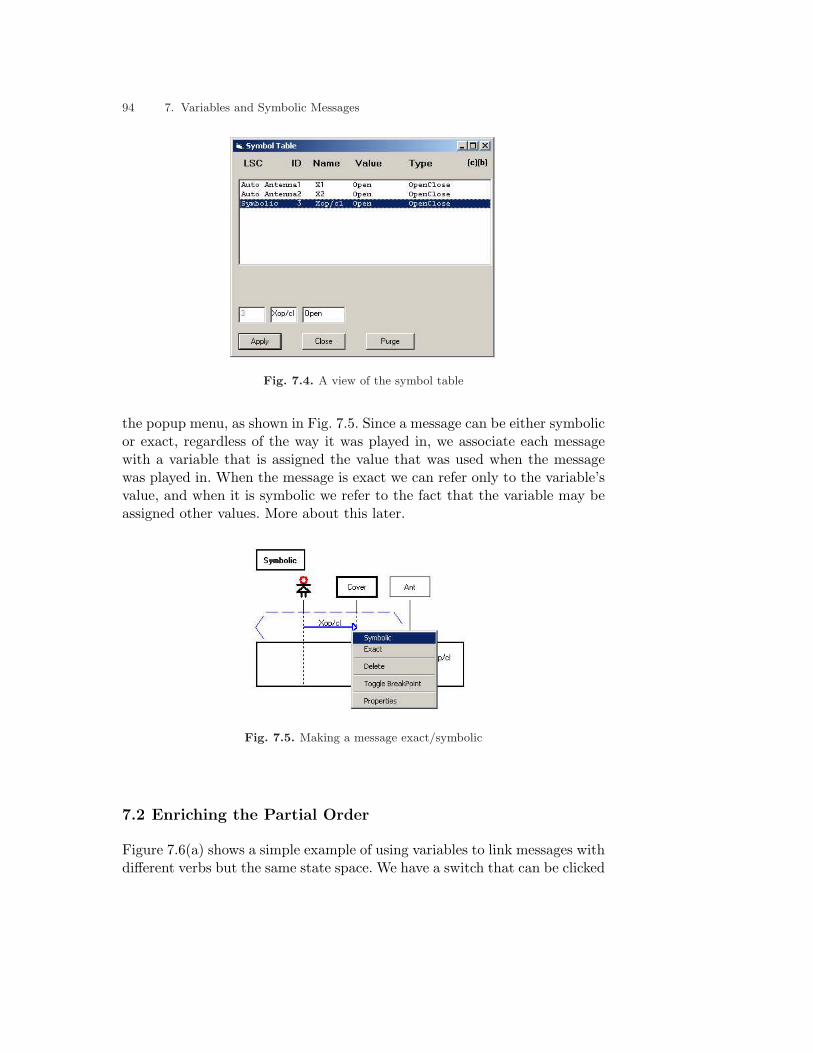
94 7. Variables and Symbolic Messages
Fig. 7.4. A view of the symbol table
the popup menu, as shown in Fig. 7.5. Since a message can be either symbolicor exact, regardless of the way it was played in, we associate each messagewith a variable that is assigned the value that was used when the messagewas played in. When the message is exact we can refer only to the variable’svalue, and when it is symbolic we refer to the fact that the variable may beassigned other values. More about this later.
Fig. 7.5. Making a message exact/symbolic
7.2 Enriching the Partial Order
Figure 7.6(a) shows a simple example of using variables to link messages withdifferent verbs but the same state space. We have a switch that can be clicked

7.2 Enriching the Partial Order 95
On or Off by the user, and a light that is required to be in the same state asthe switch; when one is On, so is the other, and the same for Off. In this case,the variable Xpower is of type Power which was defined as an enumerationcontaining the values On and Off.
Fig. 7.6. The effects of variables on LSCs partial order
A careful look at Fig. 7.6(a) reveals an interesting issue concerning thepartial order defined by the chart. There is no prechart here, but the way thechart is displayed seems to say that “the user changes the state of the switchto On or Off, and the light then changes its state to be the same as thatof the switch”. However, the partial order of this LSC does not restrict theclicking of the switch to only come before the light changes its state, sincethey are not related to some common instance. This is a problem if we reallywant the first to happen before the second.
We can resolve this by introducing a control object that receives the statefrom the switch and sends it to the light (Fig. 7.6(b)), thus restricting thepartial order, as required.1 However, we most often wish to remain on ahigher, more abstract, level of specification. On the one hand we do not wantto get into the details of how information about the value of the variableis actually transferred between the objects, but on the other hand we dowant some initial event to be the first, and hence to determine the value ofthe variable, so that subsequent uses of the same variable in different placeswill have the same value. We make this possible by a slight extension of thepartial order <L induced by an LSC L, which takes into account the verticalplacing of locations that are not on the same instance line.1 Although we have not yet discussed messages going from one object to another, the given
scenario should be clear. Messages representing interactions of that kind are discussedin Chap. 14.

96 7. Variables and Symbolic Messages
If we imagine a vertical line T aligned with an LSC L, we may consider theordering of locations from top to bottom, as projected on T . See Fig. 7.7, inwhich locations l1 and l2 are not ordered by <L but are vertically ordered; wemay write l1 <V l2 for this. The partial order <L is now extended to handle
Fig. 7.7. Vertical order: l1 <V l2
the order induced by the variables. A location is said to affect a variableX if it is associated with a message that has X as its variable. A location lis the first to affect X if it is associated with the send event of a messagethat affects X, and for every other location l′ that affects X either l <L l′ orl <V l′. Now, for a location l that is the first in L to affect the variable X,we add the relation l <L l′ to the partial order <L for every other location l′
in L that affects X.This extension thus causes the first occurrence of a variable to come be-
fore all the others, but no new order is imposed on subsequent occurrences.We have decided to do this, despite the fact that one of the basic maxims ofsequence charts prescribes that the vertical order between locations on dif-ferent instance lines does not influence the semantics. However, we find thatit is very natural for users building LSCs to specify dependent events in theorder they occur, and to cause this order to be reflected in the geometry oftheir LSCs. While we do not go as far as to attach significance to the entirevertical ordering, we do think that the first occurrence of each variable is asignificant aspect of the way the user chose to enter the information, and thatif the intention is to use the element in question as a symbolic one then theuser probably meant to say “this is the first occurrence of this symbolic value,and the value given here during execution should impact later occurrences”.And, incidentally, if the requirements are played in, events that are played infirst will appear higher up in the generated LSC anyway, which is consistentwith this philosophy.
Having said all this, we should note that this decision is not sacred, andwas made for convenience. We could have required the user to specify sepa-

7.3 Playing Out 97
rately which of the minimal occurrences of each variable is the dominatingone for the purpose of receiving and distributing a value.
7.3 Playing Out
As we have seen, when playing out behavior, the user operates the GUI ap-plication and inserts various external events. These events are then matchedwith events that appear in the different LSCs and thus force the applicationto react. In the presence of symbolic variables, events cannot be matchedsimply by straightforward identification, but, rather, should be unified in amore sophisticated way.
Recall that every message is defined as having a single variable. A variablecan be either bound or free. Initially, all the variables that appear in exactmessages are bound to their initial values and all other variables are free. Wesay that a message is bound if its variable is bound, and an event is boundif its message is bound. The same goes for free messages and events. Now,in order for two events to be matched, it is not enough for them to be ofthe same type (i.e., send/recv) and to be associated with the same systemmessage; their variables should be unifiable.
Here is how the unification of two variables works: If X and Y are bothbound to the same value, they are successfully unified and if they are boundto different values, they cannot be unified. If X is bound and Y is free,then after the variables are unified Y will be bound to the value of X. Thesame applies to the case where Y is bound and X is free. If both X andY are free, they are connected via a connection list. Later, when one of thevariables in the connection list is bound to some value, all other variables inthe connection list will be bound to the same value.
Figure 7.8 shows the symbolic LSC that was previously played in, as itis activated by the user opening the cover. When placing the mouse over amessage, the current value of its variable is shown in a tooltip, and the figureshows this happening for the message in the prechart.
As a simple example, suppose one chart that contains an event e =〈m(X), Send〉, where m(X) is a message going from O1 to O2 and is as-sociated with variable X. A second chart contains e′ = 〈m(Y ), Send〉, alsofrom O1 to O2. Now, suppose that the event of O1 sending m(3) to O2 hasoccurred. There are a number of cases to consider:
• If both e and e′ are enabled in their charts, and X and Y are free, we bindX and Y to 3 and advance both charts.
• Suppose Y is already bound to the value 4. Clearly, after binding X to 3,the messages are not the same and therefore they cannot be unified. In this

98 7. Variables and Symbolic Messages
Fig. 7.8. Binding variables during play-out
case, e will be advanced and e′ will neither be advanced nor be consideredviolating.
• The last and most interesting case is when Y is free and e′ is currentlynot enabled. There are really two possibilities we could adopt here. Thefirst is to succeed in unifying e and e′, thus advancing the first chart andcausing violation of the second, and the second possibility is to fail in theunification, thus advancing the first chart and leaving the second as is.The first approach maintains that if it is possible for an event to causea violation it should be handled as if it indeed will, and the second saysthat if it is possible that an event will not cause a violation, it should behandled as if it won’t.
We have to make a decision regarding the two possible approaches in thisthird case. Our experience with many examples shows that the second ap-proach is significantly more practical. For example, suppose there is a systemwith a display that shows several warnings while running, using messages ofthe form “show(Xi)” where the Xi’s are assigned values during the execu-tion. These messages are spread throughout several charts and should notnecessarily be synchronized with each other. If the first approach is taken,whenever the display tries to show something as dictated by one chart, it willcause a violation of other charts. This limits the specification in a way thatis very difficult to overcome. Hence, we adopt the second approach.
This decision causes a distinction between positive unification, in whichwe allow variables to be bound, and negative unification, in which variablebinding is forbidden. Positive unification is used to find minimal events inprecharts that will cause the activation of new LSC copies, and also to findevents in different active charts that should be propagated simultaneously.Negative unification is used to find violating events in active LSCs, so thatonly if a violating event is already bound to a violating value will it cause a
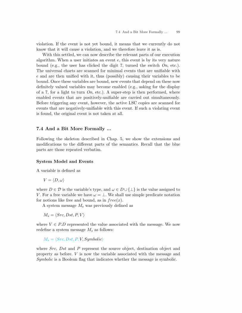
7.4 And a Bit More Formally ... 99
violation. If the event is not yet bound, it means that we currently do notknow that it will cause a violation, and we therefore leave it as is.
With this settled, we can now describe the relevant parts of our executionalgorithm. When a user initiates an event e, this event is by its very naturebound (e.g., the user has clicked the digit 7, turned the switch On, etc.).The universal charts are scanned for minimal events that are unifiable withe and are then unified with it, thus (possibly) causing their variables to bebound. Once these variables are bound, new events that depend on these nowdefinitely valued variables may become enabled (e.g., asking for the displayof a 7, for a light to turn On, etc.). A super-step is then performed, whereenabled events that are positively-unifiable are carried out simultaneously.Before triggering any event, however, the active LSC copies are scanned forevents that are negatively-unifiable with this event. If such a violating eventis found, the original event is not taken at all.
7.4 And a Bit More Formally ...
Following the skeleton described in Chap. 5, we show the extensions andmodifications to the different parts of the semantics. Recall that the blueparts are those repeated verbatim.
System Model and Events
A variable is defined as
V = 〈D, ω〉
where D ∈ D is the variable’s type, and ω ∈ D∪{⊥} is the value assigned toV . For a free variable we have ω = ⊥. We shall use simple predicate notationfor notions like free and bound, as in free(x).
A system message Ms was previously defined as
Ms = 〈Src,Dst, P, V 〉
where V ∈ P.D represented the value associated with the message. We nowredefine a system message Ms as follows:
Ms = 〈Src,Dst, P, V, Symbolic〉
where Src, Dst and P represent the source object, destination object andproperty as before. V is now the variable associated with the message andSymbolic is a Boolean flag that indicates whether the message is symbolic.

100 7. Variables and Symbolic Messages
LSC Specification
We denote by VL the set of variables that appear in an LSC L.
L = 〈IL, VL, ML, [PchL], evnt, temp〉
As shown earlier, variables have an important role in determining thepartial order of the LSC. This is captured in the following definition.
Definition 7.4.1 (affecting a variable). An LSC message M ∈ ML affectsa variable X if M.Ms.V = X.2
The notion of affecting a variable is extended to LSC events and locationsin the natural way, and we use the predicates affects(l,X) and affects(e,X)with the appropriate meanings.
We say that lix is the first location in L to affect the variable X if it affectsX, and for any other location ljy that affects X either lix <L ljy or lix <V ljy(where <V is the vertical order in L). The predicate first(l,X) is true iff l isthe first location that affects X. The partial order <L is now extended tohandle the order induced by variables as follows:
∀l, l′ ∈ `(L) : first(l, X) ∧ affects(l′, X) ⇒ l <L l′
Operational Semantics
The operational semantics remains basically the same, except that now eventshave to be unified taking variables into consideration. In Chap. 5 we definedlevel0-unifiable events.
Definition 7.4.2 (level0-unification).
1. A system event es = 〈ms, t〉 and an LSC event el = 〈ml, t′〉, with t, t′ ∈
{Send,Recv}, are level0-unifiable if t = t′, ml.Ms = ms,AppObj(ml.ISrc) = ms.Src, and AppObj(ml.IDst) = ms.Dst.
2. Two LSC events e = 〈m, t〉 and e′ = 〈m′, t′〉, with t, t′ ∈ {Send, Recv},are level0-unifiable if t = t′, m.Ms = m′.Ms, AppObj(m.ISrc) =AppObj(m′.ISrc), and AppObj(m.IDst) = AppObj(m′.IDst).
This definition is now modified so that instead of checking for equality ofmessages, the messages are checked as to whether they can be unified.2 The symbol ‘=’ is used here to denote the fact that the two arguments point to the same
variable, rather than to the fact that two different variables have the same value.

7.4 And a Bit More Formally ... 101
Definition 7.4.3 (variable unification). We say that the two variables Xand Y are positively-unifiable if X.ω = Y.ω or free(X) or free(Y ). We saythat X and Y are negatively-unifiable if X.ω = Y.ω 6= ⊥.
Definition 7.4.4 (message unification). Two system messages Ms =〈Src,Dst, P, V, Symbolic〉 and M ′
s = 〈Src′, Dst′, P ′, V ′, Symbolic′〉 are Q-unifiable, where Q is ‘positively’ or ‘negatively’, if Src = Src′, Dst =Dst′, P = P ′, and V and V ′ are Q-unifiable.
Definition 7.4.5 (level1-unification).
1. A system event es = 〈ms, t〉 and an LSC event el = 〈ml, t′〉, with
t, t′ ∈ {Send, Recv}, are Q-level1-unifiable (where Q is ‘positively’ or‘negatively’) if t = t′, and ml.Ms and ms are Q-unifiable.
2. Two LSC events e = 〈m, t〉 and e′ = 〈m′, t′〉, with t, t′ ∈ {Send, Recv},are Q-level1-unifiable if t = t′, and m.Ms and m′.Ms are Q-unifiable.
¿From now on, when we use the term unification without specifying whetherit is positive or negative, it should be read as positive unification.
As events occur in the system, LSC events are checked to see if theycan be unified, and if so their variables are actually bound to new valuesaccording to the unification process. If both variables are free, no bindingoccurs and the two variables are connected in a connection set, as describedbelow. Such a set contains variables that should be assigned to the same value.The connection sets are stored in collections called unification contexts untilthey can be bound to some value. Here is how a pair of variables is added tosuch a context:
Connect(X, Y, Context)
1. Create a connected pair in the context:
S ← {X,Y }; Context ← Context ∪ {S}
2. If X or Y are already connected, join the sets:
if ∃SX ∈ Context, s.t. X ∈ SX , then S ← S ∪ SX ;Context ← Context \ {SX}
if ∃SY ∈ Context, s.t. Y ∈ SY , then S ← S ∪ SY ;Context ← Context \ {SY }
Binding a variable in Context with a given value entails binding all thevariables in its connection set, and is done as follows:

102 7. Variables and Symbolic Messages
Bind(X, Val, Context)
1. Let SX be the set in Context s.t. X ∈ SX .2. Assign values to all variables in the set:
∀U ∈ SX : U.ω ← V al
Context ← Context \ {SX}With these last two definitions in mind, we now describe the unification
procedure:
Unify(X, Y, Context)
1. If X.ω = ⊥ ∧ Y.ω 6= ⊥ then set X.ω ← Y.ω.2. If X.ω 6= ⊥ ∧ Y.ω = ⊥ then set Y.ω ← X.ω.3. If X.ω = ⊥ ∧ Y.ω = ⊥ then Connect(X, Y, Context).4. If X.ω 6= ⊥ then Bind(X, X.ω,Context).5. If Y.ω 6= ⊥ then Bind(Y, Y.ω, Context)
We use Unify(M,M ′, Context) as an abbreviation ofUnify(M.V,M ′.V ′, Context), and Unify(e, e′, Context) as an abbreviation ofUnify(e.M, e′.M ′, Context).
Finally, the transition relation ∆ is modified to consider variables and toassign values to them as a part of executing events.
• If e = 〈M, t〉 (where t ∈ {Send, Recv}) then:1. Set Context ← ∅.2. If ∃CL ∈ RL and ∃e′ ∈ CL.LSC such that e and e′ are negatively
level1-unifiable and e′ violates CL, then set RL ← RL \ {CL}. Iftemp(CL.Cut) = hot, set Violating ← True.
3. For every universal LSC L ∈ SU which has in its prechart a minimalevent e′, positively level1-unifiable with e, create a copy of L, CL, andset RL ← RL ∪ {CL}. Set CL.Mode = PreActive and set its cut byCL.Cut ← AdvanceCut(InitialCut(L), 〈PchL, Start〉). Unify the vari-ables of e and e′, by Unify(e, e′, Context).
4. For every copy CL ∈ RL which has an enabled event e′, positively level1-unifiable with e, set its cut by CL.Cut ← AdvanceCut(CL.Cut, e′).Then, if e′ = 〈M,Send〉, M is synchronous and e′′ = 〈M,Recv〉, setthe cut by CL.Cut ← AdvanceCut(CL.Cut, e′′). Unify the variables of eand e′, by Unify(e, e′, Context).
• If e = Completed(CL) for some CL ∈ RL, then set RL ← RL \ {CL}.• If e = 〈PchL, End〉 for some CL ∈ RL, then set
CL.Cut ← BeginMainCut(CL.LSC) and CL.Mode ← Active.

7.5 Bibliographic Notes 103
7.5 Bibliographic Notes
The notion of unification was first described by Robinson in [103]. The proce-dures for message unification described in this chapter are somewhat similarto the unification of clauses in Prolog [23, 69, 118].

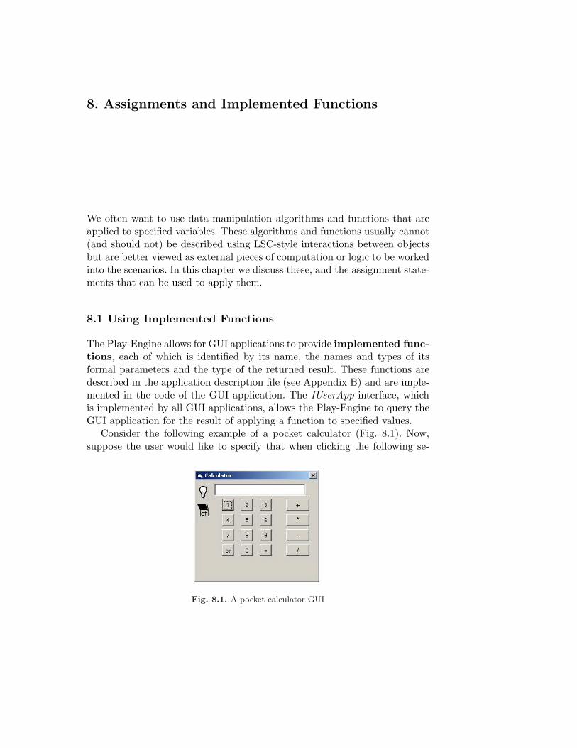
8. Assignments and Implemented Functions
We often want to use data manipulation algorithms and functions that areapplied to specified variables. These algorithms and functions usually cannot(and should not) be described using LSC-style interactions between objectsbut are better viewed as external pieces of computation or logic to be workedinto the scenarios. In this chapter we discuss these, and the assignment state-ments that can be used to apply them.
8.1 Using Implemented Functions
The Play-Engine allows for GUI applications to provide implemented func-tions, each of which is identified by its name, the names and types of itsformal parameters and the type of the returned result. These functions aredescribed in the application description file (see Appendix B) and are imple-mented in the code of the GUI application. The IUserApp interface, whichis implemented by all GUI applications, allows the Play-Engine to query theGUI application for the result of applying a function to specified values.
Consider the following example of a pocket calculator (Fig. 8.1). Now,suppose the user would like to specify that when clicking the following se-
Fig. 8.1. A pocket calculator GUI

106 8. Assignments and Implemented Functions
quence of keys, ‘X1’, ‘+’, ‘X2’ and ‘=’ in that order, where X1 and X2 areany digits, the display should show the value of X1 + X2.
The prechart is specified by entering symbolic mode and clicking the abovesequence using any digits for X1 and X2. The result is shown in Fig. 8.2.
Fig. 8.2. Prechart for summing two digits
In the main chart, the user now has to specify how the display shows X1+ X2. He/she right-clicks the GUI’s display and chooses the Value propertyfrom the popup menu. Now, instead of entering a fixed value or choosing anexisting variable, the user clicks the Function button. As a result, a list ofall the functions is shown and the user may choose one of them (see Fig. 8.3).
Continuing with our example, the user chooses the ‘+’ function,1 andthe Function button is replaced with a description of the selected function,consisting of its name and formal parameters. The user now instantiates eachof the formal parameters with an actual one, by placing the mouse cursor onthe parameter and selecting an option from the list that appears (see Fig.8.4).
The options From LSC and Variable allow the user to select a variablefrom the current LSC or from the symbol table, as described in Chap. 7.The New Value option will be discussed shortly. The user instantiates thetwo formal parameters Num1 and Num2 with the actual parameters X1 andX2, respectively, and clicks on OK. Figure 8.5 shows the final LSC for thesummation of two digits.
Recall that in Chap. 7 we said that the two messages containing X1 andX2 were affecting the variables X1 and X2, respectively. In contrast to the1 Even though the summation operation is simple and could have been provided by the
Play-Engine itself, we consider it, for the sake of the example, as a function taken fromthe application domain, which could not be provided by a general purpose tool.

8.1 Using Implemented Functions 107
Fig. 8.3. Choosing an implemented function
Fig. 8.4. Options for instantiating a function parameter
notion of affecting a variable, we introduce the notion of using a variable. Amessage is using a variable X if X must be bound before the message canbe sent. In our example, the last message, showing X1 + X2 on the display,uses the variables X1 and X2. The difference between affecting a variableand using it is that in the first case the variable can be bound to a concretevalue as the message occurs, because of unification, whereas in the secondcase the value has to be known for the message to take place.
Note that the label of the last message shows X1+X2 and not +(X1, X2).An implemented function that has exactly two parameters may be referredto as a binary operation. This is done by setting an attribute — IsBinary —to true. This attribute has no semantical meaning and is cosmetic. Binary

108 8. Assignments and Implemented Functions
Fig. 8.5. Summing two digits
operations are written as Arg1 Op Arg2 instead of the standard functionrepresentation Op(Arg1, Arg2).
8.2 Assignments
Suppose the user wishes to specify now that when the ‘×’ button is clickedtwice, the value that is currently displayed is squared and the result is shown.For the purpose of this example, we assume that the behavior for displayingnumbers as digit keys are clicked is handled by different LSCs (i.e., we areguaranteed that after clicking ‘1’, ‘2’ and ‘3’, the display will show “123”).
The user begins playing in, and while in the prechart he/she clicks the ‘×’button twice. Now, the user has to somehow refer to the currently displayedvalue. Note that the events that cause the display to change as digits areclicked are not in this LSC and therefore there is no predefined variable thatcan be referred to.
For this purpose, we introduce an assignment construct into the LSClanguage. Using an assignment, the user may save values of the properties ofobjects, or of functions applied to variables holding such values. The assigned-to variable stores the value for later use in the LSC. The expression on theright-hand side of the assignment contains a constant value, a reference to aproperty of some object (this is the typical usage) or a function applied tosome predefined variables.
In our case, we would like to store the current value property of the display.This is done by right-clicking the GUI’s display, and choosing Store and thenValue from the popup menu. Since after storing a value we might like torefer to it later, and for this a meaningful name is helpful, the Play-Engineallows the user to name the assigned variable; here we use Num (see Fig.

8.2 Assignments 109
8.6). Figure 8.7 shows the appropriate assignment statement generated inthe LSC’s prechart.
Fig. 8.6. Storing the value of an object’s property
Fig. 8.7. The assignment construct
In order to specify the result of the computation, the user moves to themain chart and, as described earlier, selects the display’s value property toshow the PowerOf function. This function has two parameters, Base and Exp,and it returns BaseExp as a result. The user instantiates the first parameterby choosing From LSC and clicking on the assignment. As a result, the Base

110 8. Assignments and Implemented Functions
parameter is replaced by Num. For the second parameter, we wish to specifythe constant ‘2’. To do this, the user places the mouse over Exp and choosesNew Value (see Fig. 8.8). As a result, a dialog is opened where a new value
Fig. 8.8. Binding a parameter to a constant
can be entered, in this case 2. After closing the dialog, the user is promptedfor a meaningful name for the variable holding this value. The name may beany string, and in this case we simply set the variable’s name to “2”.
After naming the variable, a final popup message appears, in which theuser is asked whether this variable should be treated as a non-symbolic con-stant? By saying ‘yes’ (as should be done in this example), the user specifiesthat this variable should remain bound to its original value, even if the mes-sage it appears in is symbolic. The final LSC for raising a number to thepower of 2 is shown in Fig. 8.9.
Fig. 8.9. An LSC for Num2
It is important to note that the assignment’s variable is local to the con-taining chart and can be used in the specification of that chart only, asopposed to the system’s state variables (i.e., object properties), which maybe used to communicate values between charts.

8.3 Playing Out 111
Assignments can also be used to store constant values or values returnedby implemented functions. To insert such assignments, the user clicks theappropriate button on the toolbar, chooses a name for the assigned-to variableand fills the assignment details in the dialog that is opened (see Fig. 8.10).Using this dialog, the user may specify a function, as described earlier, or
Fig. 8.10. Storing fixed values or function results
just enter a fixed value. Since the creation procedure of assignments of thiskind is not started by clicking a GUI object, the assignment is not associatedautomatically with an object instance. In order to associate the assignmentwith an object, the user right-clicks the object that should be synchronizedwith this assignment and chooses Synchronized from the popup menu.
Each assignment may have several participating objects that synchronizeat the location of the assignment. Synchronizing at an assignment means thatnone of the synchronized instances may progress beyond the assignment untilall of them reach it and it is actually performed.
8.3 Playing Out
When playing out behavior, assignments are performed according to the par-tial order induced by the LSC. In assignments, like in messages, we distinguishbetween affecting a variable and using a variable. An assignment affects itsassigned-to variable and uses all the variables in its right-hand side expres-sion. The location of an assignment in the partial order is determined by thevertical order of the instance locations attached to it and by the variablesused by it (e.g., S := X + 1 comes after the first message that affects X or

112 8. Assignments and Implemented Functions
after the first assignment that assigns a value to X, so that when it is eval-uated X is already bound). Since assignments are now another legal form ofbinding a variable to a value, an assignment that affects a variable X is alsoconsidered when looking for the first location that affects this variable.
Assignments are hidden events, since they do not correspond directly toevents carried out by the system. Therefore, when building a tool that mon-itors system runs and/or executes the LSC specification, one has to decidewhen to perform assignments. The three options considered were:
1. Perform the assignment as soon as it is enabled; that is, when all instancesthat are synchronized with the assignment have reached it and all thevariables in the right-hand side expression are bound.
2. Perform the assignment as late as possible, where the latest point anassignment can be performed is immediately before one of its subsequentevents occurs. For example, if an assignment is synchronized with twoinstances I1 and I2, and if the event following the assignment in I1 isreceiving a message and that message is indeed received, then only atthat time will the assignment be performed.
3. Choose at random a point in the interval starting when the assignment isenabled and ending when one of its subsequent events occurs, and performthe assignment at that time.
We decided on the first of these. In many examples of systems we havemodeled, performing the assignment as soon as possible seemed to be themost intuitive interpretation of the LSC. This is because when specifyingreactivity, most of the time a value is stored immediately after some eventoccurs (e.g., clicking a button), and therefore performing the assignment assoon as possible guarantees that the value is not changed before it is stored.Another argument that supports this choice is that the first option is themost deterministic one, and is therefore easier to understand and follow.
We should comment, however, that by choosing the first option (or for thatmatter, any other option) as the one driving the operational semantics forthe Play-Engine, we rule out possible behaviors that would have been allowedby making other semantic choices, both when executing a model and whenmonitoring an implementation with respect to a given model. Hence there isoften more than one way to go. This is true for other such dilemmas later inthe book too. Nevertheless, such decisions are necessary when building toolsfor model execution.
Now consider the LSC in Fig. 8.11. We would like this chart to mean thefollowing:
When the light changes its state, the display should show the previousstate of the light.

8.3 Playing Out 113
Fig. 8.11. Assignments as minimal events
In the prechart of this LSC, there is one minimal event — the assignment.Again, the question of when to perform the assignment and activate the LSCarises. Since an assignment is a hidden event, we do not consider it an eventthat can activate a prechart. This is because there is no strong intuition asto when to take such a step, and a policy that tries to cover all possibleassignment values is impractical. We have therefore decided to perform theassignment ‘just before’ the next visible event occurs. Recall that a chart isactivated when one of the minimal events in it occurs.
We now refine the definition of a minimal event to include all events thathave no visible events before them according to the partial order. When suchan event is detected, the hidden events that precede it are performed and onlythen is the visible event itself considered. To sum up, LSCs are activated onlyby visible events. A visible event may activate a prechart if it is minimal withrespect to other visible events, but as soon as such an event is detected allthe hidden events that can be performed are carried out before the visibleevent is.
Performing an assignment during play-out has the effect of binding theassigned-to variable with the value of the right-hand side expression at thepoint of evaluation. If the assignment stores a value of an object’s property,the application is queried for that value. If the assignment stores the valuereturned by an implemented function, the function information (containingits name and the values of the actual parameters) is packed and sent to theGUI application, which in turn computes the function and returns the valueto the Play-Engine. The same mechanism for function evaluation applies alsowhen functions are used directly in messages.
Messages that use implemented functions should normally be symbolic.However, if the message is exact, the value returned by the function duringplay-in is kept with the message and is used in play-out, without reevaluatingthe function. The label of such an exact message will contain the value itself

114 8. Assignments and Implemented Functions
and not the string describing the function and its parameters. Assignmentsare by definition symbolic, and therefore a function on the right-hand side ofan assignment will always be reevaluated during play-out.
During play-out, symbolic messages are matched using the unificationalgorithms described in Chap. 7. Messages containing implemented functionsare unified according to the value returned by the function and not accordingto the structure of the function. Therefore, as an example, the followingmessages are all unifiable: M(4),M(X1+X2),M(Y ),M(PowerOf(Y, X1)),where X1 = 1, X2 = 3 and Y = 4.
8.4 And a Bit More Formally ...
We now show the extensions and modifications to the semantics needed tosupport implemented functions and assignments.
System Model and Events
An implemented function is defined as:
Func = Name : D1 ×D2 × . . .×Dn → DF
where Name is the function name, Di ∈ D is the type of its ith formalparameter and DF ∈ D is the type of its returned value.
An object system Sys is modified to also contain a set of implementedfunctions F :
Sys = 〈D, C,O,F〉We redefine a system message Ms to also contain function information if
a function is used:
Ms = 〈Src,Dst, P, V, f, λFf , Symbolic〉
where f ∈ F ∪ {⊥} is a function describing a new value for P , and λFf is a
function information structure, defined for f as follows:
λFf =
{(V1 ∈ f.D1, . . . , Vn ∈ f.Dn) if f ∈ F⊥ if f = ⊥
If the message uses a function f ∈ F , the structure λFf will contain variables
as actual parameters replacing the function’s formal parameters. If Ms doesnot use an implemented function, λF
f = ⊥.At this point, a message can represent a change in a property’s value using
a variable or a function to describe the new value. This variable or functionis called the message content.

8.4 And a Bit More Formally ... 115
Definition 8.4.1 (message content). The message content Λ of a messageMs is defined as:
Ms.Λ ={
Ms.λFf if λF
f 6= ⊥Ms.V otherwise
LSC Specification
An LSC L is extended to contain assignments:
L = 〈IL, VL,ML, [PchL], AL, evnt, temp〉
An assignment is defined as
A = 〈V, IA, C, P, f, λFf 〉
where V is the assigned-to variable, IA ⊆ IL is the set of instances thatare synchronized with the assignment, C ∈ (
⋃D∈D D) ∪ {⊥} is a constant
of some type in case the assignment stores a constant, and C is ⊥ if not,P ∈ (
⋃I∈IA
I.AppObj.P)∪{⊥} is the property stored in case the assignmentstores a property value, and P is ⊥ if not, f ∈ F ∪ {⊥} is a function in casethe assignment stores some function, and f is ⊥ if not, and λF
f is a functioninformation structure in case f 6= ⊥. We require that one and only one ofthe following expressions holds for each assignment:
(C 6= ⊥), (P 6= ⊥) and (f 6= ⊥)
We say that the assignment type (or simply type) of A is constant if C 6= ⊥,property if P 6= ⊥, and function if f 6= ⊥.
We extend EL, the set of LSC events in L, to contain also hidden eventsof performing assignments:
EL = ({m ∈ ML | m.Ms ∈ ΣFromUser ∪ΣToUser ∪ΣFromEnv ∪ΣToEnv}× {Send, Recv})
∪ ({m ∈ ML | m.Ms ∈ ΣSelf} × {Send})∪ (PchL × {Start, End}) ∪ {Completed} ∪ {perform(A) | A ∈ AL}
We extend the notion of affecting a variable, and distinguish betweenaffecting a variable and using a variable.
Definition 8.4.2 (affecting a variable). An LSC message M ∈ ML affectsa variable X, if M.Ms.V = X. An assignment A ∈ AL affects a variable Xif A.V = X.
116 8. Assignments and Implemented Functions
Definition 8.4.3 (using a variable). An LSC message M ∈ ML uses avariable X if X ∈ M.Ms.λ
Ff , and an assignment A ∈ AL uses a variable X
if X ∈ A.λFf .
The notions of affecting and using a variable are extended to LSC events andlocations in the natural way. By extending the above definitions to locations,the definition of the first location that affects a variable X now refers toassignments without any change.
The partial order <L is extended with the following two rules:
Variables - The first location that affects a variable precedes all other loca-tions that affect or use the variable:
∀l, l′ ∈ `(L) : first(l, X) ∧ (affects(l′, X) ∨ uses(l′, X)) ⇒ l <L l′
Synchronize at assignments - All the instances that participate in an assign-ment are synchronized there:
∀A ∈ AL, ∀lix, ljy ∈ loc(A) : lix =L ljy
Operational Semantics
The first change we apply to our operational semantics is the redefinitionof minimal events, to consider only visible events, but to also allow hiddenevents to precede them.
Definition 8.4.4 (minimal event in a chart). An event e is minimal ina chart L if there is no visible event e′ in L such that e′ <L e.
We now extend the notion of unification to apply also to functions.
Definition 8.4.5 (function unification). Two function information struc-tures λF
f and λFg are unifiable (both positively and negatively) if f(λF
f ) =g(λF
g ) (where f(λFf ) is the value of f applied to the actual parameters in λF
f ).
Definition 8.4.6 (variable-function unification). A variable X and afunction information structure λF
f are positively-unifiable if X.ω = f(λFf ) or
free(X). They are negatively-unifiable if X.ω = f(λFf ).
Definition 8.4.7 (message unification). Two system messagesMs = 〈Src, Dst, P, V, f, λF
f , Symbolic〉 andM ′
s = 〈Src′, Dst′, P ′, V ′, f ′, λFf ′ , Symbolic′〉 are Q-Unifiable (where Q is ‘pos-
itively’ or ‘negatively’) if Src = Src′, Dst = Dst′, P = P ′ and their contentsMs.Λ and M ′
s.Λ are Q-Unifiable.

8.4 And a Bit More Formally ... 117
Since message variables may bind to values returned by functions duringexecution, we add another unification procedure to handle these cases:
Unify(X, λFf , Context)
1. If X.ω = f(λFf ) then return.
2. X.ω ← f(λFf ).
3. Bind(X, X.ω, Context).
For two unifiable messages M and M ′, we use Unify(M, M ′, Context)as an abbreviation of Unify(M.Λ,M ′.Λ, Context), and Unify(e, e′, Context)remains an abbreviation of Unify(e.M, e′.M ′, Context).
Having these definitions at hand, the transition relation ∆ supports imple-mented functions with no modifications required. However, for ∆ to supportassignments, two modification are needed: (1) When a minimal visible eventis detected, all the assignments that come before it are carried out before theevent may be considered. (2) After an assignment is performed, its assigned-to variable is bound to an appropriate value according to the assignmenttype.
• If e = 〈M, t〉(where t ∈ {Send,Recv}) then:1. set Context ← ∅.2. If ∃CL ∈ RL and ∃e′ ∈ CL.LSC such that e and e′ are negatively
level1-unifiable and e′ violates CL, then set RL ← RL \ {CL}. Iftemp(CL.Cut) = hot, set Violating ← True.
3. For every universal LSC L ∈ SU which has an event e′, positively level1-unifiable with e, as a minimal event in its prechart, create a copy of L,CL, and set RL ← RL ∪ {CL}. Set CL.Mode = PreActive and set itscut by CL.Cut ← AdvanceCut(InitialCut(L), 〈PchL, Start〉). Unify thevariables of e and e′, by Unify(e, e′, Context).For each hidden event e′′ <L e′, apply ∆(e′′).
4. For every copy CL ∈ RL which has an enabled event e′, positively level1-unifiable with e, set its cut by CL.Cut ← AdvanceCut(CL.Cut, e′).Then, if e′ = 〈M,Send〉, M is synchronous and e′′ = 〈M,Recv〉, setthe cut by CL.Cut ← AdvanceCut(CL.Cut, e′′). Unify the variables of eand e′, by Unify(e, e′, Context).
• If e = Completed(CL) for some CL ∈ RL, then set RL ← RL \ {CL}.• If e = 〈PchL, End〉 for some CL ∈ RL, then set
CL.Cut ← BeginMainCut(CL.LSC) and CL.Mode ← Active.• If e = perform(A) for some A ∈ AL s.t. CL ∈ RL, then set CL.Cut ←
AdvanceCut(CL.Cut, e) and set
118 8. Assignments and Implemented Functions
A.V ←
A.C if A.Type = constantV alue(A.P ) if A.Type = propertyA.f(A.λF
f ) if A.Type = function
After having thus modified ∆, the procedures for step should be slightlymodified so that if the new value for a property is given as a function, thatfunction is computed and the new value is reflected in the system. The pro-cedure for super-step remains unchanged.
step(e)
1. Apply ∆(e).2. Change the property value according to the value in the message:
a)
O ←{
e.M.Src if M ∈ ΣToUser ∪ΣToEnv
e.M.Dst otherwise
b) P ← e.M.Pc)
V alue(O.P ) ←{
e.M.f(e.M.λFf ) if e.M.f 6= ⊥
e.M.V.ω otherwise

9. Conditions
In this chapter we discuss guarding conditions in LSCs, and the way theirbeing true or false impacts execution.
9.1 Cold Conditions
Returning to the bakery panel application, suppose our user wishes to specifythe following requirement:
When the temperature indicated by thermometer ]1 changes, it shouldbe shown on the console. If it increases beyond 70 degrees, the consolebackground color should turn red.
The LSC describing this requirement is shown in Fig. 9.1.
Fig. 9.1. Using a cold condition
The temperature is changed by the environment in the prechart, and as aresult the console shows the new temperature in the chart body. The hexagonthat follows is a condition. This one is a cold condition, denoted by a bluedashed line, and it requires the number displayed on the console to be greaterthan 70. If a cold condition is true, the chart progresses to the location that

120 9. Conditions
immediately follows the condition, whereas if it is false, the surrounding chart(or subchart; see later) is exited. In this example, if the temperature is indeedgreater than 70 degrees, execution of the chart will progress and the consolewill change to red. If the temperature is less than or equal to 70 degrees, thechart will be exited and the console will take no action.
A condition hexagon can be stretched along several instances in the LSCin order to reach those that it refers to. To distinguish these from the in-stances that do not participate in the condition’s definition or are not to besynchronized with it, we draw small semicircular connectors at the intersec-tion points of a participating instance line with the condition.
9.2 Hot Conditions
Consider now a second requirement, stating the following:
When the main switch is turned on, the first 3-state switch is auto-matically set to Med, thus activating the first oven. As a result, thetemperature must rise above 50 degrees, and only then should the firstwarning light change to green.
Fig. 9.2. Using a hot condition: first try
As a first try, consider the LSC in Fig. 9.2. In the prechart, the user clicksthe main switch to on, and as a response, in the main chart, the first switch isset to Med. A condition then follows, constraining the temperature of the firstthermometer to be greater than 50 degrees. This condition is hot, denotedby a red solid line. A hot condition must be true, otherwise the requirementsare violated. Following this condition, the first warning light changes its colorto green.

9.3 Playing In 121
Note, however, that there is no partial order between the events and thecondition in the chart body. Therefore, a scenario in which the main switchis clicked to on and as a result the light turns green, the switch is set to Medand only then does the temperature rise above 50 degrees, is a permissableone. This, of course, is not what we had in mind. We would like to impose astrict order, in which the light turns green only after the switch is set to Medand the temperature rises. We do this by synchronizing. Like assignments,conditions can also synchronize several instances. Synchronizing at a condi-tion means that none of the synchronized instances may progress beyond thecondition until all of them reach it and it is actually evaluated. In this casewe synchronize the 3-state switch and the light with the condition (see Fig.9.3). Now, there is a strict order that forces the condition to be evaluated
Fig. 9.3. Using a hot condition with synchronization
only after the switch is set to Med, and forces the light to turn green onlyafter the condition evaluates to true.
9.3 Playing In
In order to play in a condition, the user clicks on the appropriate Conditionbutton on the toolbar. In response, a condition dialog opens (see Fig. 9.4).In our current implementation, we support conjunctive-query conditions,namely ones that are conjunctions of basic expressions. Accordingly, eachexpression that is played in is attached as a new conjunct to the conditionbeing constructed.
There are several kinds of basic expressions and different ways of playingthem in, but the play-in methods are similar to the way properties are playedin outside conditions. For example, to specify that the switch should be on,

122 9. Conditions
Fig. 9.4. A condition dialog
the user simply clicks it to on (if it is already on, the user can turn it off and onagain). When operating objects that way, the resulting expression is alwaysgenerated as an equality. To specify other kinds of relations, or to constrainobjects that cannot be operated by the user (e.g., light, thermometer, etc.)the user right-clicks the object and selects the property to be constrained. Inresponse, a basic expression dialog opens, in which the user may specify thevalue and the Boolean operator. Figure 9.5 shows the condition dialog afterthe switch was clicked to on, and the basic expression dialog, in which thecolor of the first warning light is constrained to be anything but green.
Fig. 9.5. Specifying a basic expression

9.3 Playing In 123
As described earlier, an object can participate in a condition withouthaving any of its property values actually constrained. This is usually donewhen we want the object’s progress to be synchronized with the condition’sevaluation, but to have no effect on its value. Synchronizing an object witha condition (i.e., making the object a non-influential part of the condition) isdone by right-clicking the object and choosing Synchronized from the popupmenu (see Fig. 9.6). Figure 9.7 shows the resulting condition in the LSC.
Fig. 9.6. Synchronizing an object with a condition
Since we attach importance to the intuitive manner of the play-in process,we have tried to have the user interact directly with the GUI application asmuch as possible. One example of this is in the way conditions are shown.When the user points to a condition in an LSC, several things show up; seeFig. 9.7. Within the LSC itself the condition is highlighted, as are all theparticipating instances, and the current true/false value of the condition isshown. At the same time, the GUI application (the bakery panel in our case)highlights the objects that participate in the condition, and each of themdisplays a tool tip that contains a description of the object’s part in thecondition. Since the rectangular tool tips may overlap, we have used a layoutalgorithm to arrange them nicely on the screen. This is done by defining anattractive force between each object and its tip and a repulsive force betweenevery two tips, and then letting the physics of equilibrium do the rest.
Conditions may also contain basic expressions that do not refer directlyto object properties. To specify such an expression, the user clicks on the Newbutton in the condition dialog and as a result a condition expression dialogopens (see Fig. 9.8). Using this dialog, the user may constrain the value

124 9. Conditions
Fig. 9.7. Pointing to a condition
Fig. 9.8. Possible expressions in a condition
of some variable in the LSC. A variable (like an object property) can beconstrained with respect to a constant value, another variable or a functionapplied to some variables. In this example, T1 is required to be greater thanthe value of 50 degrees Celsius converted to Fahrenheit.
In addition, there are some reserved words that can be used in conditions.A condition consisting only of the reserved word TRUE, synchronized withseveral instances, can be used to create a synchronization point for theseinstances with no other effect, because it is guaranteed to evaluate to true.Since this method for synchronizing objects is quite useful, we allow the useof the word SYNC, which is semantically equivalent to TRUE but better reflectsthe purpose of the condition.

9.3 Playing In 125
A condition consisting of the reserved word FALSE is guaranteed to fail,and as such is useful in specifying anti-scenarios, i.e., scenarios that are notallowed to happen. This is achieved by placing the forbidden scenario in theprechart and the hot condition FALSE as the sole element in the chart body.If the forbidden scenario is successfully completed, the chart is activated andthe hot condition is encountered. Since this hot condition can never be met, itcauses a violation. The overall effect is to forbid the scenario in the prechart.
In addition to reserved words, one can write any string expression asa conjunct within a condition. Since such expressions have no semanticalmeaning, when such a condition is encountered during play-out, the user isasked whether the condition holds or not, and the run progresses accordingly.(The Time option shown in the dialog of Fig. 9.8 is discussed in Chap. 16.)
A condition may contain a SELECT basic expression, which is associatedwith a probability. During play-out it evaluates to true with that probabilityand to false with the complement probability. Although the main use ofthe select statement is within if-then-else constructs, as discussed in Chap.10, it can be useful also in stand-alone guards. The LSC in Fig. 9.9 showssuch an example. In this LSC, after the switch is clicked to on, the light
Fig. 9.9. Specifying nondeterministic behavior
turns on with a probability of 50%. Combining a select expression with astandard expression as a conjunctive condition results in a guarded select, inwhich progress is allowed with a given probability only if the guard (i.e., thestandard expression) holds.
Expressions that do not refer to object properties are not automaticallyassociated with object instances, and therefore a condition consisting solelyof such expressions must be explicitly synchronized with some object.

126 9. Conditions
9.4 Playing Out
When playing out behavior, conditions are very much like assignments. Theyare performed according to the partial order induced by the LSC, and arealso considered hidden events.
In contrast with assignments and messages, conditions cannot affect vari-ables but can only use them. A condition uses all the variables that appearin its basic expressions. The location of a condition in the partial order isdetermined therefore by the vertical order of the instance locations attachedto it and by the variables it uses. For example, X > f(Y ) can be evaluatedonly after the messages that affect X and Y are sent or after the assignmentsthat assign values to them are performed, so that when the expression isevaluated, X and Y are already bound.
Conditions are hidden, since they do not correspond directly to eventscarried out by the system. Therefore, the same decisions we had to make forthe execution of assignments must be made for conditions. With conditions,the number of options is even greater since the temperature of the conditionand its value may affect the decision about whether to advance it or not.
The case of hot conditions is easy. Since a hot condition must be true, whenit is reached it is constantly evaluated and is advanced if and when it becomestrue. The execution will remain stuck at that point if the specification isincorrect and the condition indeed never becomes true. Recalling that anti-scenarios are expressed using a hot false condition in the main chart, thereis no point in the engine waiting for a hot condition consisting of the wordFALSE to become true; the chart is therefore viewed as causing an immediateviolation, and in the Play-Engine implementation it is crossed out and aviolation message pops up (see Fig. 9.10).
Obviously, we could have used theorem-proving techniques to find other,less trivial, everywhere-false conditions and treat them as immediate viola-tions too, but this is beyond the scope of our research. We have implementedonly the most basic and practical feature needed to support the expressionand detection of anti-scenarios.
Turning now to cold conditions, one can think of several possible policiesfor executing them, such as waiting for them to be true if they are currentlyfalse or waiting for them to be false if currently true, and deciding at randomwhether to evaluate them or evaluating them immediately. We have chosenthe policy where cold conditions are evaluated immediately, mainly becausethis seems more intuitive for users to follow. In Chap. 16 we shall see thatthere are ways to explicitly require a condition to be evaluated only after acertain delay.
Let us consider now the two LSCs of Fig. 9.11. Both of these LSCs state

9.4 Playing Out 127
Fig. 9.10. Detecting anti-scenarios
Fig. 9.11. Conditions in precharts
that if the Probe button is clicked while the switch is on, the console shouldshow “Probing ...”.
There is however a difference between the charts. In ‘LSC1’ the minimalevent is the message (this is a synchronous message and therefore we referto it as an event consisting of both the sending and the receiving), whilein ‘LSC2’ the minimal event is that of evaluating the condition. If we use‘LSC1’, the chart will be activated as soon as the button is clicked, and ifthe switch is Off the prechart is violated, which means that the chart stopsexisting since its triggering scenario is not fulfilled (see Fig. 9.12).
Conditions appearing as minimal events are treated again like assign-ments, because of the same considerations of intuition and practicality. Whena visible event is detected, the conditions that precede it are evaluated andonly then is the event considered. There is however a difference between as-signments and conditions. A minimal assignment can always be performed,thus allowing the visible event to be considered, while in order for a condition

128 9. Conditions
Fig. 9.12. Prechart violation
to be advanced its value must be true. Returning to ‘LSC2’ in Fig. 9.11, ifthe button is clicked while the switch is Off, the visible event of clicking thebutton in the chart cannot be reached because the instances cannot progressbeyond the condition, and therefore the chart will not be activated at all.Actually, in order to evaluate the condition, assignments that may precede itshould be performed. It is thus semantically inaccurate to say that the chartis not activated at all; it is better to say that the actions are taken ‘behindthe scenes’ without the user being aware of them.
A prechart with the event coming before the condition, as in ‘LSC1’, canbe used to indicate that after some visible event occurs progress dependson some condition, while a prechart like ‘LSC2’ is used to indicate that apre-condition must hold in order for the event to even be considered.
9.5 And a Bit More Formally ...
Following the semantics skeleton, we show the extensions and modificationsneeded to support conditions.
System Model and Events
Conditions are entirely specification oriented, and therefore do not affect thesystem model.
LSC Specification
An LSC L is extended to contain conditions:
L = 〈IL, VL,ML, [PchL], AL, CL, evnt, temp〉A condition C in an LSC L is defined as
9.5 And a Bit More Formally ... 129
C = 〈IC , Ψ〉
where IC ⊆ IL is the set of instances that are synchronized with the conditionand Ψ is the set of basic expressions. A basic expression ψ ∈ Ψ is definedover the following alphabet:
ψ ∈ {LHS ×Oper ×RHS} ∪ {TRUE, FALSE, SELECT(P),⊥}where
LHS ∈ {O.P |O ∈ O, P ∈ O.P} ∪ VL
Oper ∈ {=, <,≤, >,≥, 6=}RHS ∈ (
⋃
D∈DD) ∪ VL ∪ {(f, λF
f )|f ∈ F}
The first kind of expression is used to constrain a property or a variable, bycomparing it via some comparison operator with a constant value, anothervariable or a function. The second kind of expression consists of the reservedwords (SYNC is really just an abbreviation for TRUE), the SELECT statementwith probability P , and free expressions (all free expressions are reduced to⊥). We denote by value(ψ) the result of evaluating ψ in the natural way.If ψ is of the form SELECT(P), a Boolean value is chosen at random withprobability P for true, and if ψ is ⊥ the user is prompted for a value. Thevalue of a condition C is defined as:
value(C) =∧
ψ∈Ψ
value(ψ)
Since conditions may also be cold or hot, the domain of the function tempshould be modified:
temp : `(L) ∪ML ∪ CL → {hot, cold}
We extend EL, the set of LSC events in L, to contain also hidden eventsof evaluating conditions:
EL = ({m ∈ ML | m.Ms ∈ ΣFromUser ∪ΣToUser ∪ΣFromEnv ∪ΣToEnv}× {Send,Recv})∪ ({m ∈ ML | m.Ms ∈ ΣSelf} × {Send})∪ (PchL × {Start, End}) ∪ {Completed} ∪ {perform(A) | A ∈ AL}∪ {eval(C) | C ∈ CL}
The definition of using variables is modified to reflect the way conditions usethem.
130 9. Conditions
Definition 9.5.1 (using a variable). An LSC message M ∈ ML uses avariable X if X ∈ M.Ms.λ
Ff , and an assignment A ∈ AL uses a variable X
if X ∈ A.λFf .
A condition basic expression ψ uses a variable X if at least one of thefollowing holds:
1. ψ.LHS ∈ VL and ψ.LHS = X.2. ψ.RHS ∈ VL and ψ.RHS = X.3. ψ.RHS = (f, λF
f ) and X ∈ λFf .
A condition C uses a variable X if one of its basic expressions uses it.
The partial order <L is now extended with the following rule:
Synchronize at conditions - All the instances that participate in a conditionare synchronized there:
∀C ∈ CL, ∀lix, ljy ∈ loc(C) : lix =L ljy
Operational Semantics
Since conditions are pretty much like assignments in the sense that theyare hidden events that are not considered as minimal events, most of thedefinitions remain unchanged.
There is however one change in the definition of enabled events, whichmakes sure that false hot conditions are not evaluated unless they explicitlycontain the basic expression FALSE.
Definition 9.5.2 (enabled event). An event e is enabled with respect toa cut C if »(¼C ∪ loc(e)) is a legal cut. That is, if the location in C of everyinstance participating in the event e is the one exactly prior to e, and thereis no e′ <L e that is not already in the down-closure of C.
• If e = 〈m,Send〉, m is synchronous and e′ = 〈m,Recv〉, we require alsothat ¼C∪loc(e)∪loc(e′) is down-closed, thus making sure that a synchronousmessage will not be sent unless it can be received.
• If e = eval(C), temp(C) = hot and FALSE /∈ C.Ψ , we require also thatvalue(C) = true.
Next, ∆ is extended with transitions for handling the evaluation of con-ditions:
• If e = 〈M, t〉 (where t ∈ {Send, Recv}) then:1. Set Context ← ∅.

9.5 And a Bit More Formally ... 131
2. If ∃CL ∈ RL and ∃e′ ∈ CL.LSC such that e and e′ are negativelylevel1-unifiable and e′ violates CL, then set RL ← RL \ {CL}. Iftemp(CL.Cut) = hot, set Violating ← True.
3. For every universal LSC L ∈ SU which has an event e′, positively level1-unifiable with e, as a minimal event in its prechart, create a copy of L,CL, and set RL ← RL ∪ {CL}. Set CL.Mode = PreActive and setits cut by CL.Cut ← AdvanceCut(InitialCut(L), 〈PchL, Start〉). Unifythe variables of e and e′, by Unify(e, e′, Context). For each hidden evente′′ <L e′, apply ∆(e′′).
4. For every copy CL ∈ RL which has an enabled event e′, positively level1-unifiable with e, set its cut by CL.Cut ← AdvanceCut(CL.Cut, e′).Then, if e′ = 〈M,Send〉, M is synchronous and e′′ = 〈M,Recv〉, setthe cut by CL.Cut ← AdvanceCut(CL.Cut, e′′). Unify the variables of eand e′, by Unify(e, e′, Context).
• If e = Completed(CL) for some CL ∈ RL, then set RL ← RL \ {CL}.• If e = 〈PchL, End〉 for some CL ∈ RL, then set
CL.Cut ← BeginMainCut(CL.LSC) and CL.Mode ← Active.• If e = perform(A) for some A ∈ AL s.t. CL ∈ RL, then set CL.Cut ←
AdvanceCut(CL.Cut, e) and set
A.V ←
A.C if A.Type = constantV alue(A.P ) if A.Type = propertyA.f(A.λF
f ) if A.Type = function
• If e = eval(C) for some C ∈ CL s.t. CL ∈ RL, then1. If value(C) = true then set CL.Cut ← AdvanceCut(CL.Cut, e);2. If value(C) = false then set RL ← RL \ {CL}. If temp(C) = hot, set
Violating ← True.
Since false hot conditions that do not explicitly contain the expressionFALSE are not enabled, and all other conditions should be evaluated as soonas they are enabled, the procedure super-step remains unchanged, with theemphasized part taking care also of conditions:

132 9. Conditions
super-step
1. Compute the set of enabled events:
Enabled ←⋃
CL∈RL{e ∈ EL|enabled(e)}
Enabled ← Enabled \ External
2. If there is a hidden enabled event e ∈ Enabled, thena) Apply ∆(e).b) Go back to 1.
3. If there is a visible enabled event e ∈ Enabled, such that e doesnot violate any copy which is in active mode, thena) step(e).b) Go back to 1.
4. Terminate super-step.
9.6 Bibliographic Notes
Conjunctive queries were first defined in [20]. An algorithm for synthesiz-ing UML statecharts from UML sequence diagrams is presented in [119]. Itmakes use of constraints written in OCL [115] (the UML object constraintslanguage), which are of the form V ar = V alue. These constraints are usedto resolve conflicts arising from different scenarios and to join system statesthat identify over these variables; they can be viewed as a sort of combinationof our assignments and conditions.
The layout algorithm we have used for the tool tips is a variant of thenon-uniform vertex graph layout algorithm of [45], adapted to arrange a setof arbitrary rectangles in the plane.
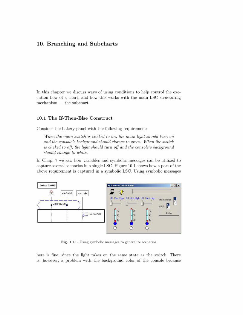
10. Branching and Subcharts
In this chapter we discuss ways of using conditions to help control the exe-cution flow of a chart, and how this works with the main LSC structuringmechanism — the subchart.
10.1 The If-Then-Else Construct
Consider the bakery panel with the following requirement:
When the main switch is clicked to on, the main light should turn onand the console’s background should change to green. When the switchis clicked to off, the light should turn off and the console’s backgroundshould change to white.
In Chap. 7 we saw how variables and symbolic messages can be utilized tocapture several scenarios in a single LSC. Figure 10.1 shows how a part of theabove requirement is captured in a symbolic LSC. Using symbolic messages
Fig. 10.1. Using symbolic messages to generalize scenarios
here is fine, since the light takes on the same state as the switch. Thereis, however, a problem with the background color of the console because

134 10. Branching and Subcharts
there is no direct link between the state of the switch and the color of theconsole.1 What we need here is a construct for conditional choice, which willmake it possible to perform different scenario fragments, depending on somecondition. Figure 10.2 shows how the problem is solved using an if-then-elseconstruct.
Fig. 10.2. Conditional choice using if-then-else
An if-then-else construct consists of two adjacent subcharts — the ‘then’part and the ‘else’ part — and a controlling condition that is located at thetop of the first subchart. The operational semantics is the standard condi-tional branching. The ‘else’ part is not mandatory and may be omitted.
10.2 Subcharts
A subchart, as its name suggests, is a well-formed fragment of a chart. Itis rendered as a thick solid rectangle stretching over all the instances thatare involved in the scenarios it contains, and is not restricted to appear aspart of an if-then-else construct. Lines of instances that are geometricallylocated in the area of the subchart but do not participate in it are not shownin the subchart (they are hidden behind it). The beginning and end of asubchart are synchronization points for all participating instances. Thus, asubchart is entered only after all the instances that participate in it arrive atthe locations associated with the subchart start.1 In this case such a link could be represented by an implemented function that takes
an On/Off value as a parameter and returns a green/white color as a result, yet this iscumbersome and there are many cases where such links cannot be established.

10.3 Nondeterministic Choice 135
This fact can be reason enough to use the subchart construct in the firstplace. For example, Fig. 10.3 shows an LSC containing two subcharts. Bysurrounding the pairs of events with subcharts, we guarantee that the twoevents in the first pair will both occur before those in the second pair. A
Fig. 10.3. Subcharts in LSCs
subchart is exited only after all the instances have completed their activitiesin it, with one exception, which we discuss next.
In the previous chapter, we said that when a cold condition evaluates tofalse the chart is exited. We now extend this definition. If a cold conditionresiding within a subchart evaluates to false, the closest surrounding subchartis exited. If there is no surrounding subchart, the chart itself is exited (as inthe original definition).
Entering a subchart and exiting it are considered hidden events that areperformed as soon as possible. Carrying out these events has no effect on thesystem model or on the values of LSC variables. Their only effect is to movethe cut beyond the subchart start/end line for all participating instances.
10.3 Nondeterministic Choice
In Chap. 9 we introduced the select statement, used as a basic expression inconditions. In this section we show how a select statement within an if-then-else construct can be used to specify nondeterministic choice.

136 10. Branching and Subcharts
Fig. 10.4. Specifying a nondeterministic choice
The LSC in Fig. 10.4 specifies that when the user clicks the switch toon, the background color of the console turns green with probability 50%and blue with probability 50%. When executing this LSC, the Play-Enginerandomly picks a value from {true, false} with the specified probabilities,executing the ‘then’ part or the ‘else’ part accordingly.
10.4 Playing In
To play in a subchart construct, the user clicks the Subchart button on thetoolbar. In response, the Play-Engine opens a subchart wizard and placesthe cursor automatically in the subchart rectangle (see Fig. 10.5). The user
Fig. 10.5. A wizard for specifying subcharts
then simply continues playing in the scenario fragment that should be lo-cated in the subchart. Clicking the End Subchart button closes the subchartconstruct and the cursor is placed immediately after it.

10.4 Playing In 137
In order to play in an if-then-else construct, the user clicks the If-Then-Elsebutton on the toolbar. In response, the Play-Engine opens an if-then-else wiz-ard and a condition dialog (see Fig. 10.6). The first thing the user does is
Fig. 10.6. A wizard for specifying if-then-else constructs
to specify the condition using the methods and techniques described in theprevious chapter. The Play-Engine then places the cursor automatically inthe ‘then’ part and the user simply continues playing in the subchart thatshould be satisfied when the condition holds (see Fig. 10.7(a)). To specify the
Fig. 10.7. Playing in an if-then-else

138 10. Branching and Subcharts
‘else’ part, the user clicks on Specify the ELSE part in the wizard and theengine creates the ‘else’ subchart and moves the cursor there in preparationfor playing in the rest of the construct (see Fig. 10.7(b)). Clicking the END IFbutton closes the if-then-else construct and the cursor is placed immediatelyafter it.
10.5 Playing Out
When executing an LSC specification, the condition of an if-then-else con-struct is evaluated as soon as all the instances that participate in the con-struct have reached it, assuming that the condition itself can be evaluated(all the variables it uses are bound). If the condition evaluates to true thePlay-Engine executes the ‘then’ subchart, and if it evaluates to false the ‘else’subchart is executed. In the example given in Fig. 10.2, as soon as the lightchanges its state, the condition is evaluated and the background color of theconsole changes to green or white, depending on the state of the light.
If-then-else constructs are handled somewhat differently when they appearin precharts. Consider the LSC in Fig. 10.8. The scenario in the prechart can
Fig. 10.8. An if-then-else in a prechart
be read in two different ways. According to the execution semantics describedabove, it reads:
Wait for the user to click the main switch to on. Immediately afterthat, check the temperature indicated by thermometer ]1. If it is below50 degrees, (enter the ‘then’ part and) wait for the user to set the

10.5 Playing Out 139
state of the first 3-state switch to High. If the temperature is at least50 degrees, (enter the ‘else’ part and) wait for the user to set the stateof the first 3-state switch to Med.
Thus, the condition of the if-then-else is evaluated an a priori unknown periodof time before any of the events in the ‘then’ or ‘else’ parts occur.
We have chosen a different semantics for an if-then-else appearing in theprechart. According to our proposed semantics, the scenario of Fig. 10.8reads:
Wait for the user to click the main switch to on. Then, wait for theuser to (i) set the state of the first 3-state switch to High while thetemperature indicated by thermometer ]1 is below 50 degrees, or (ii)set the state of the first 3-state switch to Med while the temperatureis at least 50 degrees.
Here, we evaluate the condition as the event occurs, thus linking the eventto a context in which the condition holds. The approach is similar to andconsistent with the one we adopted for evaluating minimal cold conditionsin precharts. We believe that this interpretation of if-then-else constructsappearing in precharts is more intuitive and fits better with the way peoplethink when specifying conditional choices in a triggering scenario.
If-then-else constructs are the first constructs we have seen so far thatbehave differently when monitored in a prechart and when executed in thechart body. This subtle difference in the semantics, and hence in the executionmechanism, evolves from the poignant difference between monitoring andexecution.
When executing an LSC specification, the play-out mechanism is respon-sible for generating visible events, and in the case of the Play-Engine alsofor reflecting the effects of these events in the GUI representation of the sys-tem model. Hence, when an if-then-else construct is encountered in a chartbody, the execution mechanism should evaluate the condition and continuegenerating any events that depend on the condition’s value.
In contrast, events in precharts are monitored in order to see if the prechartcan be successfully completed. Since the order of events and their timingis a priori unknown, the prechart monitoring mechanism should enable theprechart to be completed if possible. The evaluation of a condition is a hiddenevent and its timing is not dictated by the system itself, therefore choosingto evaluate it as soon as possible will eliminate one of the courses that canbe taken by the system (e.g., evaluating a condition when it is true, and thesystem later producing an event matching the case of the condition beingfalse). When monitoring a system, the visible events are produced by thesystem itself. Therefore, the monitoring mechanism should wait for the next

140 10. Branching and Subcharts
event from the system and let that event dictate the choice between the ‘then’and the ‘else’ parts, since it is that event that reflects the choice made by thesystem.
One could argue that there are more options for the scheduling of condi-tion evaluation, which our semantics does not cover. For example, there couldbe a case where the condition holds at time T1, later at time T2 it becomesfalse, and at T3 becomes true again. Finally, at time T4, the system generatesan event that belongs to the ‘else’ part. In this case, neither of the policiesof evaluating the condition as soon as possible or as late as possible willmonitor the if-then-else construct to completion. To overcome this, we couldset things up so that the monitoring mechanism continuously monitors thecondition and probably maintains two copies for the two options. However,since a prechart can have more than one if-then-else construct enabled simul-taneously (referring to different objects), the number of copies needed to bemaintained can easily blow up. Apart from the fact that monitoring mecha-nisms that try to cover all options are not practical, they lack the intuition,according to which the event is linked with the system context (conditionvalue) in which it occurs.
Figure 10.9 shows a nondeterministic choice in the prechart. As discussed
Fig. 10.9. Nondeterministic choice in a prechart
above, a condition in an if-then-else construct that appears in a prechartis evaluated only when one of the minimal events in the ‘then’ part or the‘else’ part occurs. The same holds for nondeterministic choice in prechartstoo, but with one exception. When the Play-Engine monitors a prechartwith a nondeterministic choice, it does not randomly choose the part tobe monitored, but, rather, ‘agrees’ with any choice made by the system.

10.6 And a Bit More Formally ... 141
Therefore, in this example, the Play-Engine waits for the console to changeits background to green or blue, and according to the event taken by thesystem the Play-Engine enters the correct part of the choice. Note that whenit comes to monitoring charts, the actual value of the probability that isattached to a select statement has no meaning; it just states that the twooptions are possible.2
The differences between monitoring an LSC specification and executing itare discussed in more detail in Chap. 12.
10.6 And a Bit More Formally ...
Following the semantics skeleton, we show the extensions and modificationsneeded to support branching and subcharts.
System Model and Events
Subcharts and if-then-else constructs are entirely specification oriented andtherefore do not affect the system model.
LSC Specification
An LSC L is now extended to contain subcharts and if-then-else constructs:
L = 〈IL, VL,ML, [PchL], AL, CL, SUBL, ITEL, evnt, subchart, temp〉
where SUBL is the set of subcharts in L, ITEL is the set of if-then-elseconstructs in L and subchart is a mapping function.
Every LSC construct can be contained in at most one immediately sur-rounding subchart. The function subchart returns for each construct the in-nermost subchart to which it belongs (if there is no such subchart it returns⊥). The domain of subchart includes SUBL, thus enabling nested subcharts:
subchart : ML ∪AL ∪ CL ∪ SUBL → SUBL ∪ {⊥}
The function subchart is extended to events and to instance locations in thenatural way. We will also use the notation e ∈ Sub as an abbreviation ofsubchart(e) = Sub.
The set of instances ISub participating in a subchart Sub is defined as theset of all instances that are involved in some activity in Sub:2 If, however, a probability of 0% or 100% is specified, then only the events in the corre-
sponding subchart are allowed to occur.

142 10. Branching and Subcharts
ISub = {I ∈ IL| ∃M ∈ ML s.t. (subchart(M) = Sub∧ (I = M.ISrc ∨ I = M.IDst))∨ ∃A ∈ AL s.t. (subchart(A) = Sub ∧ I ∈ IA)∨ ∃C ∈ CL s.t. (subchart(C) = Sub ∧ I ∈ IC)∨ ∃Sub′ ∈ SUBL s.t. subchart(Sub′) = Sub ∧ I ∈ ISub′}
An if-then-else construct ITE in L is defined as:
ITE = 〈IITE , C, SubT , SubE〉where IITE = IC ∪ ISubT
∪ ISubEis the set of instances participating in the
if-then-else construct, C is the main condition of the if-then-else construct,SubT ∈ SUBL is the subchart containing the ‘then’ part and SubE ∈ SUBL∪{⊥} is the subchart containing the ‘else’ part (and if there is no such part,SubE = ⊥).
We extend EL, the set of LSC events in L, to contain also hidden eventsof entering subcharts and exiting them and a special event for branching inan if-then-else construct:
EL = ({m ∈ ML | m.Ms ∈ ΣFromUser ∪ΣToUser ∪ΣFromEnv ∪ΣToEnv}× {Send,Recv})
∪ ({m ∈ ML | m.Ms ∈ ΣSelf} × {Send})∪ (PchL × {Start, End}) ∪ {Completed}∪ {perform(A) | A ∈ AL} ∪ {eval(C) | C ∈ CL}∪ (SUBL × {Start, End}) ∪ {branch(ITE)| ITE ∈ ITEL}
We have to cater for the need to exit an if-then-else construct fromsomewhere within one of its subcharts. For this we use the virtual event(ITE, End), defined as:
(ITE, End) ,{
(ITE.SubE , End) if ITE.SubE 6= ⊥(ITE.SubT , End) if ITE.SubE = ⊥
The partial order <L is extended with the following rules:
Synchronize at subcharts - All the instances that participate in a subchartare synchronized at its start and end.
∀Sub ∈ SUBL, ∀lix, ljy ∈ loc((Sub, Start)) : lix =L ljy
∀lix, ljy ∈ loc((Sub,End)) : lix =L ljy
If-then-else branch - All the events in an if-then-else construct may be carriedout only after the main condition has been evaluated and one of the ‘then’or ‘else’ branches has been selected.
∀ITE ∈ ITEL, ∀e ∈ ITE.SubT ∪ ITE.SubE : branch(ITE) <L e

10.6 And a Bit More Formally ... 143
We must also remove from the relation <L all the pairs of locations thatbelong to different parts of an if-then-else construct, so that events that arein the ‘else’ part are not considered as coming after events in the ‘then’ part:
Disconnect If and Else - Events in ‘then’ subcharts should not be consideredas preceding events in ‘else’ subcharts.
∀ITE ∈ ITEL, ∀lix, liy s.t. lix ∈ ITE.SubT ∧ liy ∈ ITE.SubE : lix ≮L liy
Operational Semantics
If-then-else constructs are the first constructs we have seen so far that behavedifferently when monitored in a prechart and when executed in the chartbody. To correctly monitor if-then-else constructs within precharts, we shouldallow the execution mechanism to ‘wait’ outside the construct until a minimalevent in the ‘then’ part or the ‘else’ part occurs. In order to allow waitingoutside the if-then-else construct but to enable events inside its subcharts tooccur, we extend the range of occurrences of events allowed, to include morethan the set of directly enabled ones.
Definition 10.6.1 (reachable event). A visible event e is reachable froma cut C if:
1. The event e is enabled with respect to C, or2. There exists a hidden event e′ such that e is reachable from the cut C ′ =
AdvanceCut(C, e′).
The reachable events are therefore all the events that are enabled, or canbecome enabled by propagating some hidden events.
The transition relation ∆ is therefore extended with transitions for han-dling if-then-else constructs and with transitions allowing reachable eventsto occur, even if they are not directly enabled:
• If e = 〈M, t〉 (where t ∈ {Send, Recv}) then:1. Set Context ← ∅.2. If ∃CL ∈ RL and ∃e′ ∈ CL.LSC such that e and e′ are negatively
level1-unifiable and e′ violates CL, then set RL ← RL \ {CL}. Iftemp(CL.Cut) = hot, set Violating ← True.
3. For every universal LSC L ∈ SU which has an event e′, positively level1-unifiable with e, as a minimal event in its prechart, create a copy of L,CL, and set RL ← RL ∪ {CL}. Set CL.Mode = PreActive and setits cut by CL.Cut ← AdvanceCut(InitialCut(L), 〈PchL, Start〉). Unifythe variables of e and e′, by Unify(e, e′, Context). For each hidden evente′′ <L e′, apply ∆(e′′).

144 10. Branching and Subcharts
4. For every copy CL ∈ RL which has a reachable event e′, positively level1-unifiable with e, set its cut by CL.Cut ← AdvanceCut(CL.Cut, e′).Then, if e′ = 〈M,Send〉, M is synchronous and e′′ = 〈M,Recv〉, setthe cut by CL.Cut ← AdvanceCut(CL.Cut, e′′). Unify the variables ofe and e′, by Unify(e, e′, Context). For each hidden event e′′ <L e′, apply∆(e′′).
• If e = Completed(CL) for some CL ∈ RL, then set RL ← RL \ {CL}.• If e = 〈PchL, End〉 for some CL ∈ RL, then set
CL.Cut ← BeginMainCut(CL.LSC) and CL.Mode ← Active.• If e = perform(A) for some A ∈ AL s.t. CL ∈ RL, then set
CL.Cut ← AdvanceCut(CL.Cut, e) and set
A.V ←
A.C if A.Type = constantV alue(A.P ) if A.Type = propertyA.f(A.λF
f ) if A.Type = function
• If e = eval(C) for some C ∈ CL s.t. CL ∈ RL, then1. If value(C) = true then set CL.Cut ← AdvanceCut(CL.Cut, e);2. If value(C) = false then
a) If subchart(C) ∈ {ITE.SubT , ITE.SubE} for some ITE then
set CL.Cut ← AdvanceCut(CL.Cut, (ITE,End))
b) If subchart(C) = Sub ∈ SUBL then
set CL.Cut ← AdvanceCut(CL.Cut, (Sub, End))
c) If subchart(C) = ⊥ then set RL ← RL \ {CL};d) If temp(C) = hot, set Violating ← True.
• If e = branch(ITE) for some ITE ∈ CL s.t. CL ∈ RL then1. If value(ITE.C) = true then set
CL.Cut ← AdvanceCut(CL.Cut, (ITE.SubT , Start));2. If value(ITE.C) = false then
set CL.Cut ←{
AdvanceCut(CL.Cut, (ITE.SubE , Start)) if ITE.SubE 6= ⊥AdvanceCut(CL.Cut, (ITE.SubT , End)) if ITE.SubE = ⊥
• If e = (ITE.SubT , End) for some ITE ∈ CL s.t. CL ∈ RL then
set CL.Cut ← AdvanceCut(CL.Cut, (ITE,End))
• If e = (ITE.SubE , End) for some ITE ∈ CL s.t. CL ∈ RL then
set CL.Cut ← AdvanceCut(CL.Cut, (ITE.SubE , End))

10.6 And a Bit More Formally ... 145
• If e = (Sub, End) for some Sub ∈ CL s.t. CL ∈ RL then
set CL.Cut ← AdvanceCut(CL.Cut, (Sub, End))
Finally, we modify super-step so it does not attempt to evaluate conditionsof if-then-else constructs that are located in precharts (i.e., within copies thatare preactive).
super-step
1. Compute the set of enabled events:
Enabled ←⋃
CL∈RL{e ∈ EL | enabled(e)}
Waiting ←⋃
CL ∈ RL,CL.Mode = PreActive
{e | e = branch(ITE)}
Enabled ← Enabled \ (External ∪Waiting)
2. If there is a hidden enabled event e ∈ Enabled, thena) Apply ∆(e).b) Go back to 1.
3. If there is a visible enabled event e ∈ Enabled, such that e doesnot violate any copy which is in active mode, thena) step(e).b) Go back to 1.
4. Terminate super-step.

146 10. Branching and Subcharts
10.7 Bibliographic Notes
The MSC standard also describes a higher-level way of connecting MSCs,termed hierarchical MSCs (HMSCs). An HMSC is a directed graph with oneinitial node and one final node. Each node in the graph is associated with abasic MSC (bMSC). Using HMSCs, one can specify the order in which differ-ent scenario fragments are to be considered, similar to the way it is done withsubcharts in LSCs. HMSCs also allow one to define conditions as nodes of theunderlying graph, thus allowing for conditional branching, where each branchis given as a bMSC or an HMSC. A major difference between a subchart inan LSC and a bMSC in an HMSC lies in the synchronization requirement.In LSCs, all the instances that participate in a subchart synchronize at itsbeginning and end, while in HMSCs there is no such requirement. The factthat an instance is allowed to proceed to the next bMSC without having tosynchronize with other instances has some significant effects on behavior, asdiscussed in Chap. 13.

Part IV
Advanced Behavior: Multiple Charts


11. Executing Multiple Charts
In previous chapters we presented various LSC constructs. Besides discussingthe play-in process for each construct, we also discussed its semantics whenmonitoring a system against an LSC specification, and then showed how itcan be played out directly within its host LSC. However, the focus so far wason the semantics of the construct within a single LSC. An LSC specificationwill typically consist of a number (often a large number) of charts, and play-out’s most subtle issues arise from their combination and interaction. In thischapter we focus on executing multiple LSCs, as well as on overlappingincarnations of a single LSC.
11.1 Simultaneous Activation of Multiple Charts
Consider the two LSCs of Fig. 11.1. They describe different actions requiredto be taken by the system when the main switch is clicked to on. ‘LSC1’states that the main light should turn on, and ‘LSC2’ states that the firstswitch should be set to Med and the first warning light should turn green.
As the user plays out a scenario in which the main switch is clicked to on,both charts are activated. Suppose that these charts are not to be executed,but rather are viewed as a test of a system, meaning that they are to bemonitored against a sequence of events generated by the system. In this case,all the Play-Engine has to do is to wait for the next event, advance thecharts accordingly and check that the partial order induced by the charts isnot violated. In contrast, suppose that the charts are to be executed by thePlay-Engine, and there is no other system against which we are testing. Inthis case, the engine has to choose the next event and must then proceed tocarry it out. In the above example, the three events can be chosen in anyorder, since they are not constrained by the LSC partial order.
Suppose now that, in addition to the two LSCs of Fig. 11.1, the specifi-cation also contains the LSC shown in Fig. 11.2, stating that when the user

150 11. Executing Multiple Charts
Fig. 11.1. Activating two LSCs as a result of a single event
clicks the main switch to on, the main light turns on, and only after that canthe first switch and the warning light take their actions.1
Fig. 11.2. Constraining events in other charts
1 This kind of phenomenon, where different scenarios refer to the same set of actionsand reactions in a somewhat different way, is quite common when preparing systemrequirements, where it is often the case that they are written by more than one personor in several phases.

11.1 Simultaneous Activation of Multiple Charts 151
Now, when the user clicks the switch to on, the three charts are activated.In this case, the only event that can be carried out without getting intotrouble is that of turning on the light, since selecting any one of the other twoevents will cause a violation of ‘LSC3’. Accordingly, the algorithm underlyingthe play-out mechanism has been designed to allow the choice of the nextevent to be carried out only from among the set of events that are bothenabled and do not violate any other chart.
We have seen several examples of LSCs that were activated by (i.e., theirprecharts contained) user actions. LSCs can also be activated by systemevents, thus enabling the specification of scenario fragments that maybe shared by more than one scenario. The LSC ‘Med-Green1’ in Fig. 11.3(a)states that when the first 3-state switch is set to Med, the first warning lightchanges to green. Another LSC, ‘Green1-Console’, shown in Fig. 11.3(b),states that every time the first warning light changes to green, a correspond-ing message appears on the console.
Fig. 11.3. Activation of one LSC by another
When the user sets the state of the first 3-state switch to Med during play-out, ‘Med-Green1’ is activated. Since its prechart contains only one message,it is successfully completed and the Play-Engine executes the event in thechart body. As this event is fired, it is identified as a minimal event in theprechart of ‘Green1-Console’ and this chart is activated too (see Fig. 11.4).The LSC event selected by the Play-Engine is marked by a thick red circleand all the events that are advanced simultaneously with it (in this case thereis only one) are marked by thin red circles.
Sometimes, in order to progress with the execution dictated by the body ofcertain LSCs, we must violate the precharts of others. Consider for example aspecification that contains an LSC for each pair of switch and warning light,saying that when the former is set to Med, the latter turns green. Suppose wehave another chart saying that if the warning lights turn green in ascending

152 11. Executing Multiple Charts
Fig. 11.4. Chain of activations in play-out
order, from 1 to 3, the console should display some message. Now, assumethat the user clicks switch number 1 and then switch number 3. Figure 11.5shows the result. After setting the first switch to Med, the first light turns
Fig. 11.5. Violating a prechart
green and activates the LSC ‘All Green’ (on the right). When the user thensets the state of the third switch to Med, the Play-Engine has to select anevent to carry out. In this case, the only enabled event is that of changingthe third light to green, but clearly this event is not enabled in the LSC ‘AllGreen’. Precharts can obviously stay active without being completed, andunless and until a prechart is completed, the system is not constrained bythe corresponding LSC at all. Thus, the Play-Engine is allowed to change

11.1 Simultaneous Activation of Multiple Charts 153
the color of the third light to green and terminate the prechart before it iscompleted.
A careful examination of the issue of violating an LSC before its prechartcompletes raises the following question: why not try to violate all prechartsas soon as possible, thus minimizing the set of constraints imposed on theexecution. Indeed, this is a legitimate question, and a policy that selectsevents based on this criteria would have been a legitimate one. This kindof policy is minimal, in the sense that it minimizes the set of events thatshould be carried out, by trying to ‘cut off’ LSCs that do not yet obligatethe execution.
We have chosen a maximal policy; i.e., our algorithm tries to avoid vio-lating precharts as long as it can. Only if there is no choice left and the onlyevents that can be carried out are ones that violate some prechart, is suchan event taken and the prechart terminated. This rule applies not only toprecharts. The play-out algorithm may also violate LSC copies that are inactive mode and are located in a cold cut. Again, we allow this, since violat-ing an LSC in a cold cut is not considered a violation, due to the fact thatnone of the instances is obligated to progress. Therefore, when an event vio-lating such a chart is taken, it can be viewed as though the instances decidedto stay in their locations and the chart could have been terminated earlier.Similarly, our reluctance to violate precharts also carries over to cold cuts ofthe main chart. This is also due to the maximal approach we take.
The principle behind the maximal approach is the following: We believethat users specify behavior for a reason, and they want the behavior to beexecuted if possible. Cold cuts are means to allow scenarios to end beforethey are expected, due to possible interactions with other scenarios.
To summarize, the play-out execution mechanism searches for enabledevents to be carried out according to the following order:
1. If there is an enabled event that does not violate any prechart or anyLSC in a cold cut, select it.
2. If there is an event that violates some prechart but does not violate anyLSC in a cold cut, select it.
3. If there is an enabled event that violates an LSC in a cold cut but doesnot violate any LSC in a hot cut, select it.
4. Otherwise, no event can be carried out.
In the Play-Engine, the user is given full control over whether or not toallow violation of precharts and whether to allow violation of cold cuts whenlooking for the next event (i.e., whether to allow the Play-Engine to use steps2 and 3 when it looks for the next event to be carried out).
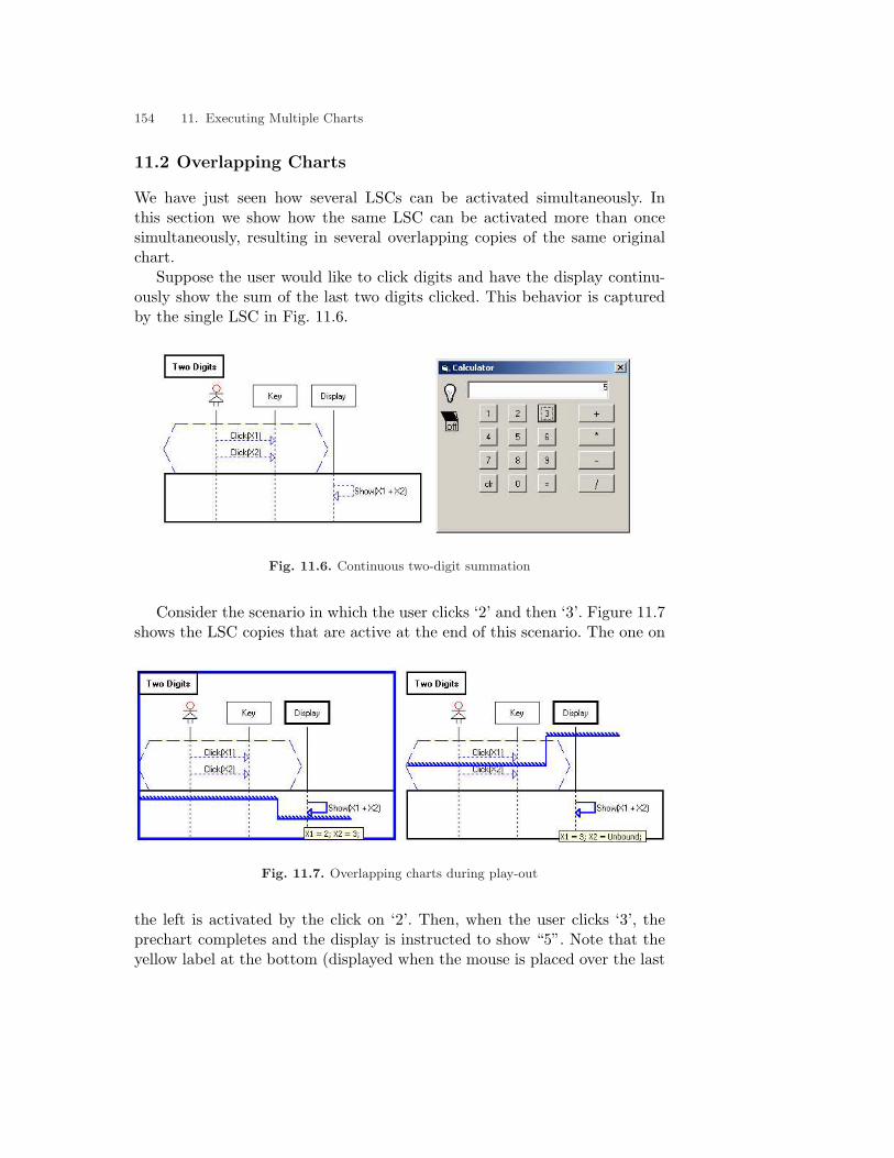
154 11. Executing Multiple Charts
11.2 Overlapping Charts
We have just seen how several LSCs can be activated simultaneously. Inthis section we show how the same LSC can be activated more than oncesimultaneously, resulting in several overlapping copies of the same originalchart.
Suppose the user would like to click digits and have the display continu-ously show the sum of the last two digits clicked. This behavior is capturedby the single LSC in Fig. 11.6.
Fig. 11.6. Continuous two-digit summation
Consider the scenario in which the user clicks ‘2’ and then ‘3’. Figure 11.7shows the LSC copies that are active at the end of this scenario. The one on
Fig. 11.7. Overlapping charts during play-out
the left is activated by the click on ‘2’. Then, when the user clicks ‘3’, theprechart completes and the display is instructed to show “5”. Note that theyellow label at the bottom (displayed when the mouse is placed over the last

11.2 Overlapping Charts 155
message) shows that X1 and X2 are bound to 2 and 3, respectively. Anotherthing that occurs as a result of the user clicking ‘3’ is the activation of a newcopy of the same LSC, the reason being that clicking ‘3’ is unifiable with aminimal event in the chart. The new copy is shown on the right in Fig. 11.7,and, as can be seen, it is waiting for the next digit to be clicked before itsprechart can be completed. The tool tip in this LSC copy shows that X1 isbound to 3 and X2 is still unbound.
The fact that an LSC can be active simultaneously in several copies,each in a different cut, can be used for several purposes. One interestinguse involves recursive calls. Consider the LSCs in Fig. 11.8, which consti-tute a scheme of a recursive computation consisting of a start, a recursivecall guarded by a termination condition, and some way of specifying the re-turned value. Figure 11.8(a) shows that when a digit is clicked, the display’sbackground changes to white and it then shows the digit itself. Figure 11.8(b)
Fig. 11.8. Recursion in LSCs

156 11. Executing Multiple Charts
consists of the recursive call. It says that every time the display shows somevalue, if this value is greater than 1 a new value equal to the previous valueminus two is shown. The recursion stems from the fact that the event ofdecreasing the digit in the body of the chart of Fig. 11.8(b) triggers a rein-carnation of that very chart, as long as the digit shown is larger than 1.Finally, the LSC of Fig. 11.8(c) says that when the display shows the value0 or 1 its background changes to green or red, respectively. Besides loopingdown and decreasing the display digit, this combination of LSCs checks par-ity without the use of odd or even predicates: when an even digit is clickedthe display turns green, and when the digit clicked is odd the display turnsred.
Figure 11.9 shows a snapshot of the active LSCs towards the end of a run.Figure 11.9(a) shows the ‘Recursive Call’ LSC that was activated when the
Fig. 11.9. Recursive LSCs during play-out
display showed “2”. Since the variable X5 in this copy is bound to 2, thecold condition holds and the display is instructed to show “0” (marked by athick red circle). As a result of this event, two more charts are activated. Anew copy of ‘Recursive Call’ is created, this time with X5 bound to 0 (Fig.11.9(b)). In this LSC the cold condition does not hold and therefore the chainof recursive calls terminates. In addition, the LSC ‘Terminate’ is activatedwith D = 0. The cold condition in the prechart of this LSC is true andthe main chart is entered. The main condition of the if-then-else evaluatesto true, causing the background of the display to change to green and thescenario to end.

11.3 And a Bit More Formally ... 157
Figure 11.10 shows how the two LSCs of Fig. 11.8(b) and 11.8(c) can becombined using nested if-then-else constructs. It is clear that this LSC can
Fig. 11.10. More compact recursion
replace the two original charts, but what is particularly interesting is thefact that all three can be executed together, synchronizing on all the visibleevents they share.
In the above examples we saw that a single LSC can be active in morethan one copy simultaneously. We should emphasize that different copies ofthe same LSC do not differ only in their cuts but also in the values assignedto their variables. Thus, an LSC live copy consists of a fully cloned chart,including an independent copy of its variables. We would also like to notethat although the example of recursion seems a bit coarse, it is because wehave used messages that denote property changes. In Chap. 14 we refine thesystem model with messages that better capture the notion of calling anobject or sending it a control signal.
11.3 And a Bit More Formally ...
The issue of executing multiple charts is not related to the system modelor to the LSC language, and is therefore relevant only to the operationalsemantics.

158 11. Executing Multiple Charts
Operational Semantics
The notions of enabled events and violating events were defined in previouschapters and remain unchanged. The procedure for performing a super-stepreferred to these definitions too and avoided carrying out events that violatedother LSCs. We now refine super-step so that it tries to avoid selecting eventsthat violate other precharts or LSCs in cold cuts. The operational semanticsassumes that both kinds of violation are permissable and does not refer tothe option of the user controlling these parameters. The extension is quitestraightforward.
super-step
1. Compute the set of enabled events:
Enabled ←⋃
CL∈RL{e ∈ EL|enabled(e)}
Waiting ←⋃
CL ∈ RL,CL.Mode = PreActive
{e | e = branch(ITE)}
Enabled ← Enabled \ (External ∪Waiting)
2. If there is a hidden enabled event e ∈ Enabled, thena) Apply ∆(e).b) Go back to 1.
3. If there is a visible enabled event e ∈ Enabled, such that e doesnot violate any copy that is in active or preactive mode, thena) step(e).b) Go back to 1.
4. If there is a visible enabled event e ∈ Enabled, such that e doesnot violate any copy that is in active mode, thena) step(e).b) Go back to 1.
5. If there is a visible enabled event e ∈ Enabled, such that e doesnot violate any copy that is in active mode with a hot cut, thena) step(e).b) Go back to 1.
6. Terminate super-step.

12. Testing with Existential Charts
Universal charts, which must be satisfied by any run that satisfies theirprechart, ‘drive’ the model by their action/reaction nature. In contrast, ex-istential charts, which can get by with only a single satisfying run, can beused as system tests or as examples of object interactions. In this chapter,we deal with the uses of existential charts and the way they are monitoredby the Play-Engine.
12.1 Specifying Test Scenarios
Consider Fig. 12.1, which describes the following scenario-based test:
Fig. 12.1. Specifying tests with existential charts
The user first opens the cover and dials 911 (by clicking the digitkeys in that order). At this point, the display is expected to change its

160 12. Testing with Existential Charts
mode from Date to Number and should display the number “ 911”.Next, the user clicks the Send button. At this point the speaker shouldemit an outgoing dial tone. Then, when a signal indicating that thecall was answered (denoted by the word ACK) is received from theenvironment, the speaker becomes silent.
In contrast to universal charts, this LSC does not specify how and whenthe system actions are carried out (e.g., displaying a number, making a sound,etc.), but rather constrains the behavior of the system to satisfy a set ofconditions that are expected to hold at different points in the run. We areusing it to define a test scenario. The required test results are specified usinghot conditions, thus enabling the chart to complete only if the conditions allevaluate to true.
Although system tests can be described using existential charts, it is im-portant to remember that a system can satisfy an existential LSC by produc-ing but a single run in which the LSC is successfully traced to completion.Therefore, in the case of nondeterministic systems, satisfying an existentialLSC cannot be considered as proving that the system always behaves in someway, but only that it may behave in some way. To show that a system al-ways behaves in a specified manner, one should monitor the system againsta universal LSC.
12.2 Monitoring LSCs
Rather than serving to drive the play-out, existential charts are monitoredand checked for their successful completion. To integrate the monitoring capa-bilities into our execution mechanism, recall from Sect. 5.3 that an executionengine had to satisfy the first four requirements. We now add a fifth, yieldingthe following list:
1. Identify an external stimulus and find all the requirements that shouldbe considered when resolving the system’s response to it (e.g., identifythe event of flipping a switch and find all the requirements that specifythe system’s responses to the switch being flipped).
2. Apply the relevant requirements to create the sequence of system reac-tions. This is done iteratively, and thus includes identifying additionalrequirements that become relevant as the system is responding and ap-plying them too (e.g., after the switch is flipped, send a signal to thecontroller, which in turn may result in sending a signal to the light andturning it on).

12.2 Monitoring LSCs 161
3. Identify scenarios that are forbidden according to the requirements, andavoid generating them (e.g., make sure that if the requirements say thata certain signal cannot be sent to the light while it is on, it will indeednot be sent when the light is on).
4. If a forbidden scenario actually occurs (e.g., because some other manda-tory scenario forces it to), indicate a violation.
5. Indicate when an existential (provisional) scenario successfully completes.
When monitoring a chart, the Play-Engine simply tracks the events inthe chart as they occur, and is not required to initiate any visible eventswhile doing so. Existential charts are monitored in a way similar to thatfor monitoring precharts of universal charts. Conditions and assignments areperformed and evaluated as soon as they are enabled, while the choices be-tween ‘then’ and ‘else’ subcharts of if-then-else constructs are delayed untilan event in one of the two subcharts occurs.
When (and if) a traced chart reaches its end, it is highlighted, and theuser is informed that it was successfully traced to completion. The user mayselect the charts to be monitored in advance, thus saving the Play-Enginethe need to track charts that might currently be of no interest. Figure 12.2shows the chart from Fig. 12.1 after it was successfully traced to completion.
As with universal charts, there could be cases where a single existentialchart is activated in several overlapping copies, and at a given time duringexecution each one is in a different tracking status (i.e., in a different cut).This is fine, since one does not know a priori when a satisfying scenariobegins, and it could be the case that such a scenario begins after some prefixof it has already been monitored. Had we allowed only a single copy for eachLSC active at a time, we would definitely have missed some of the satisfyingscenarios, and erroneously concluded that some existential scenario is notsatisfiable.
Universal LSCs go through a PreActive → Active → Terminate life cycle.Existential LSCs go through a similar, though simpler, life cycle. When one ofthe minimal visible events in the chart occurs, the copy is created and entersthe Check state. If the chart is violated, it is simply exited and deleted. If itcompletes successfully, it moves through a temporary Completed state wherevarious registration and management actions are taken, and it is then exitedand deleted. Figure 12.3 shows the full life cycle of LSC copies.
Having existential LSCs at hand makes it possible to consider the notionof consistency between a system and a specification. Earlier, we defined aconsistent run as one that does not violate any universal LSC in the spec-ification. A system is consistent with a specification if all its runs are

162 12. Testing with Existential Charts
Fig. 12.2. Monitoring existential charts
consistent with the specification and, in addition, each existential LSC is sat-isfied by some run. Note that without existential LSCs, and with a passiveuser, a system could be easily consistent by simply doing nothing, since anempty run trivially satisfies all the universal charts. Of course, since univer-sal charts can have user events in their precharts, the system can be forcedto react even if no existential charts are present. However, in principle, ifwe somehow prevented the user from taking any action (e.g., by initiatingthe system with locked switches, buttons, etc.), then, in the absence of exis-tential charts, the system could do nothing and still be consistent with thespecification.
12.3 Recording and Replaying
When playing out the GUI application, a run trace is produced, which in-cludes all the user actions and the system reactions. These runs can berecorded, to provide testimonies for fulfilling existential LSCs. Figure 12.4shows a fragment of a recorded run.
Recorded runs can be saved (in XML format) and then reloaded andreplayed. In replaying a run, the user may select both existential and universal

12.3 Recording and Replaying 163
Fig. 12.3. Life cycle of LSC copies, including existential charts
charts to be traced. Existential LSCs can thus be shown to be fulfilled, andwith universal charts the run shows when the charts were activated and
Fig. 12.4. A recorded run

164 12. Testing with Existential Charts
how they participated in creating the system’s reactions. And, of course, theengine notifies us if a universal chart is violated.
More importantly, runs can be imported from different sources and re-played in the same manner. These external sources can be different imple-mentations of the specification, either given as executable programs or asmore detailed design models (e.g., statecharts, labeled transition systems,etc.). Importing a run from an implementation and replaying it, while trac-ing all charts, can be used to show that the implementation is consistent withthe requirements, in the sense that existential charts are successfully tracedand universal charts are not violated.
Recorded runs can be manipulated by the user, by changing the orderof events and checking whether the resulting run is also a legal one. One ofthe interesting possibilities that we have built into the Play-Engine is that ofdeleting all system reactions and leaving only user and environment actions.After applying this modification, the resulting run can be replayed. The usercan then specify that universal charts should also be activated (and not onlymonitored). In this case, events from the recorded run are injected as before,but now the selected universal charts activate the system and trigger eventsas specified in their bodies.
This feature may be used for regression testing, in the following way.While fulfilling (part of) the existential LSCs, the runs are recorded. Lateron, if some of the universal charts change, the runs can be modified to containonly user actions and can then be replayed to verify that existential LSCs arestill successfully fulfilled and no universal charts are violated in the process.
12.4 On-line Testing
As discussed in the previous section, in order to test an intra-object model oran actual system implementation with respect to a given LSC specification,the system should record the generated events, and the recorded run can thenbe loaded into the Play-Engine and replayed.
The Play-Engine provides another, more convenient, way for testing sys-tem models and implementations. Using an External Event Manager, thePlay-Engine can be connected through a TCP/IP connection to other pro-grams. To test a system, we would connect it to the Play-Engine and haveit send the generated events along the communication line. These events, inthe format of recorded events, would be received by the Play-Engine andinjected into the execution and monitoring mechanisms, in a way similar tohow recorded events are injected.

12.5 Executing and Monitoring LSCs in the Play-Engine 165
The Play-Engine enables the user to inject the events upon their arrivalor to have them accumulate in a queue and then inject them manually. Byasking the engine to monitor all the LSCs in the specification, the user cantest the system and verify that all the existential charts can be satisfied andno universal charts are violated in the process. By having it activate universalLSCs, the Play-Engine can operate in a mode where the external events areactually received from an external source and are used to trigger the system’sreactions, which are generated by the engine itself.
The Play-Engine can also be instructed to send the generated events backto the communication line, and thus affect the connected program in anydesired way. This feature also makes it possible to connect two Play-Engines,each executing its own specification and serving as the external environmentof the other; see Sect. 21.5.
12.5 Executing and Monitoring LSCs in the Play-Engine
Prior to LSCs, scenario-based languages were used mainly to express require-ments, which are later verified against system runs. The semantics of theselanguages is therefore oriented towards testing, and it specifies whether a setof runs generated by the system satisfies the specification. Obviously, sincethe language of LSCs can serve for testing as well, we would like to supportthis kind of semantics too. However, the fact that our main interest in thisbook is in executing some LSCs, the ones that drive the execution, while onlymonitoring others, affects the language’s operational semantics.
Figure 12.5 illustrates how an LSC specification can be used both fordriving a model and for monitoring it. When executing an LSC specification,the user may choose the LSCs that drive the model and those that will bemonitored. The driving LSCs must all be universal, while the set of moni-tored LSCs may include both existential and universal charts. To keep thesemantics clean, we require that the two sets be disjoint. In practice, thePlay-Engine allows a universal LSC to both drive the model and be moni-tored at the same time, and we refer to such cases as if there are two identicalbut distinct LSCs, one in each set.
According to the conventional semantics of scenario-based languages, theset of driving LSCs is empty and all the LSCs are monitored. In this setting,events generated by the system are monitored one after the other (usingmonitor event), by applying track event to these events and to hidden eventsbetween them. The track event procedure is the basis of the LSC semanticsand it computes all the actions that should be taken as a result of firing an
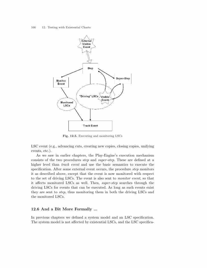
166 12. Testing with Existential Charts
Fig. 12.5. Executing and monitoring LSCs
LSC event (e.g., advancing cuts, creating new copies, closing copies, unifyingevents, etc.).
As we saw in earlier chapters, the Play-Engine’s execution mechanismconsists of the two procedures step and super-step. These are defined at ahigher level than track event and use the basic semantics to execute thespecification. After some external event occurs, the procedure step monitorsit as described above, except that the event is now monitored with respectto the set of driving LSCs. The event is also sent to monitor event, so thatit affects monitored LSCs as well. Then, super-step searches through thedriving LSCs for events that can be executed. As long as such events existthey are sent to step, thus monitoring them in both the driving LSCs andthe monitored LSCs.
12.6 And a Bit More Formally ...
In previous chapters we defined a system model and an LSC specification.The system model is not affected by existential LSCs, and the LSC specifica-

12.6 And a Bit More Formally ... 167
tion was already defined with existential LSCs in mind. Therefore, the onlymodifications that are required here are in the operational semantics.
Operational Semantics
An LSC copy of an existential LSC is in Check mode as long as it exists.
Definition 12.6.1 (LSC live copy). Given an LSC L, a live copy of L,denoted by CL, is defined as
CL = 〈LSC,Mode, Cut〉,where LSC is a copy of the original chart, Mode ∈ {PreActive, Active,Check} is the execution mode of this copy, and Cut is some legal cut ofL representing the current location of the instances of L in this particularcopy.
When executing an LSC specification, the user may choose the LSCs thatdrive the model and those that should be monitored. These two sets arerequired to be disjoint. The operational semantics is therefore given as:
Sem(S) = 〈V, V0,SD,SM , ∆[SO,SC ]〉A state V ∈ V is modified to contain not only live copies of driving LSCs
(RL) but also a set of live copies of monitored LSCs (ML):
V = 〈RL,ML,Violating〉The initial configuration contains no copies of driving LSCs and no copies ofmonitored LSCs, and is defined as:
V0 = 〈∅, ∅, False〉SD ⊆ SU is the set of driving LSCs, SM ⊆ SU ∪ SE is the set of LSCs the
user wishes to monitor, and the two sets satisfy SD ∩ SM = ∅.The transition relation ∆ is no longer applied automatically to all the
LSCs in the specification and to the sets of running copies RL, but is pa-rameterized with two sets. The first set, SO, contains original LSCs that aresubject to ∆. The second set, SC , contains the live copies that currently exist.This set contains only copies of LSCs from SO. The two sets are instantiatedwith either (SD,RL) or (SM ,ML).
Note that if one cares only about the ‘standard’ part of the semantics,i.e., the part that enables a system to be tested and verified against anLSC specification, and not in executing the specification directly, this canbe achieved by setting SM = S and SD = ∅.
The transition relation ∆[SO,SC ] is modified so that it refers to its pa-rameters and is extended to consider existential charts.

168 12. Testing with Existential Charts
• If e = 〈M, t〉 (where t ∈ {Send, Recv}) then:1. Set Context ← ∅.2. If ∃CL ∈ SC and ∃e′ ∈ CL.LSC, such that e and e′ are nega-
tively level1-unifiable and e′ violates CL, then set SC ← SC \ {CL}.If temp(CL.Cut) = hot, set Violating ← True.
3. For every universal LSC L ∈ SO which has an event e′, positively level1-unifiable with e, as a minimal event in its prechart, create a copy ofL, CL, and set SC ← SC ∪ {CL}. Set CL.Mode = PreActive and setits cut by CL.Cut ← AdvanceCut(InitialCut(L), 〈PchL, Start〉). Unifythe variables of e and e′, by Unify(e, e′, Context). For each hidden evente′′ <L e′, apply ∆(e′′).
4. For every existential LSC L ∈ SO which has an event e′, positively level1-unifiable with e, as a minimal event in the chart body, create a copy ofL, CL, and set SC ← SC ∪{CL}. Set CL.Mode = Check, and set its cutto the beginning of the chart by CL.Cut ← BeginMainCut(CL.LSC).Unify the variables of e and e′, by Unify(e, e′, Context). For each hiddenevent e′′ <L e′, apply ∆(e′′).
5. For every copy CL ∈ SC which has a reachable event e′, positively level1-unifiable with e, set its cut by CL.Cut ← AdvanceCut(CL.Cut, e′).Then, if e′ = 〈M,Send〉, M is synchronous and e′′ = 〈M,Recv〉, setthe cut by CL.Cut ← AdvanceCut(CL.Cut, e′′). Unify the variables ofe and e′, by Unify(e, e′, Context). For each hidden event e′′ <L e′, apply∆(e′′).
• If e = Completed(CL) for some CL ∈ SC , then set SC ← SC \ {CL}.• If e = 〈PchL, End〉 for some CL ∈ SC , then set
CL.Cut ← BeginMainCut(CL.LSC) and CL.Mode ← Active.• If e = perform(A) for some A ∈ AL s.t. CL ∈ SC , then set CL.Cut ←
AdvanceCut(CL.Cut, e) and set
A.V ←
A.C if A.Type = constantV alue(A.P ) if A.Type = propertyA.f(A.λF
f ) if A.Type = function
• If e = eval(C) for some C ∈ CL s.t. CL ∈ SC then1. If value(C) = true then set CL.Cut ← AdvanceCut(CL.Cut, e).2. If value(C) = false then
a) If subchart(C) ∈ {ITE.SubT , ITE.SubE} for some ITE then
set CL.Cut ← AdvanceCut(CL.Cut, (ITE,End))
b) If subchart(C) = Sub ∈ SUBL then
set CL.Cut ← AdvanceCut(CL.Cut, (Sub, End))
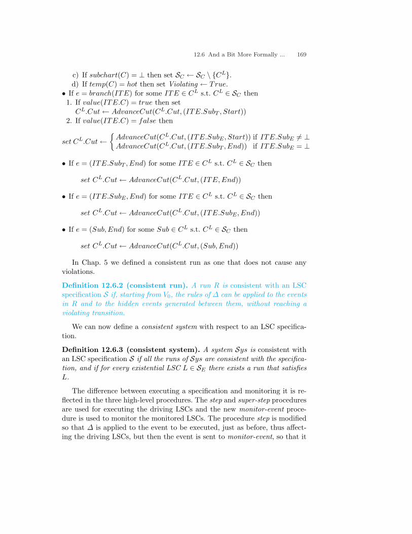
12.6 And a Bit More Formally ... 169
c) If subchart(C) = ⊥ then set SC ← SC \ {CL}.d) If temp(C) = hot then set Violating ← True.
• If e = branch(ITE) for some ITE ∈ CL s.t. CL ∈ SC then1. If value(ITE.C) = true then set
CL.Cut ← AdvanceCut(CL.Cut, (ITE.SubT , Start))2. If value(ITE.C) = false then
set CL.Cut ←{
AdvanceCut(CL.Cut, (ITE.SubE , Start)) if ITE.SubE 6= ⊥AdvanceCut(CL.Cut, (ITE.SubT , End)) if ITE.SubE = ⊥
• If e = (ITE.SubT , End) for some ITE ∈ CL s.t. CL ∈ SC then
set CL.Cut ← AdvanceCut(CL.Cut, (ITE,End))
• If e = (ITE.SubE , End) for some ITE ∈ CL s.t. CL ∈ SC then
set CL.Cut ← AdvanceCut(CL.Cut, (ITE.SubE , End))
• If e = (Sub, End) for some Sub ∈ CL s.t. CL ∈ SC then
set CL.Cut ← AdvanceCut(CL.Cut, (Sub, End))
In Chap. 5 we defined a consistent run as one that does not cause anyviolations.
Definition 12.6.2 (consistent run). A run R is consistent with an LSCspecification S if, starting from V0, the rules of ∆ can be applied to the eventsin R and to the hidden events generated between them, without reaching aviolating transition.
We can now define a consistent system with respect to an LSC specifica-tion.
Definition 12.6.3 (consistent system). A system Sys is consistent withan LSC specification S if all the runs of Sys are consistent with the specifica-tion, and if for every existential LSC L ∈ SE there exists a run that satisfiesL.
The difference between executing a specification and monitoring it is re-flected in the three high-level procedures. The step and super-step proceduresare used for executing the driving LSCs and the new monitor-event proce-dure is used to monitor the monitored LSCs. The procedure step is modifiedso that ∆ is applied to the event to be executed, just as before, thus affect-ing the driving LSCs, but then the event is sent to monitor-event, so that it

170 12. Testing with Existential Charts
affects the monitored LSCs too. Thus, a model that is driven by some chartscan simultaneously monitor other charts.
step(e)
1. Apply ∆[SD,RL](e).2. Change the property value according to the value in the message:
a)
O ←{
e.M.Src if M ∈ ΣToUser ∪ΣToEnv
e.M.Dst otherwise
b) P ← e.M.Pc)
V alue(O.P ) ←{
e.M.f(e.M.λFf ) if e.M.f 6= ⊥
e.M.V.ω otherwise
3. monitor-event(e).
Since the procedure super-step triggers the execution of events by send-ing them to step, and step already sends them to monitor-event, super-stepremains unchanged from its latest definition in Chap. 11.
In case a sequence of visible events is to be monitored against an LSCspecification, as in replaying a run, for example, the events are sent one byone to monitor-event. This procedure is a simple combination of a single stepand a super-step which is allowed to propagate only hidden events. The inputto monitor-event is a single event and it advances all the hidden events untilnone is enabled:
monitor-event(ev)
1. Apply ∆[SM ,ML](ev).2. Compute the set of enabled events:
Enabled ←⋃
CL∈ML{e ∈ EL|enabled(e)}
Waiting ←⋃
CL∈ML{e | e = branch(ITE)}
Enabled ← Enabled \Waiting
3. If there is a hidden enabled event e ∈ Enabled, thena) Apply ∆[SM ,ML](e).b) Go back to 2.
4. Terminate monitor-event.

12.7 Bibliographic Notes 171
12.7 Bibliographic Notes
The notion of a consistent system with respect to an LSC specification wasgiven in [27]. In [46] a consistent LSC specification is defined as a specificationfor which there exists a set of runs such that every existential chart is satisfiedby at least one run and every universal chart is satisfied by all runs. It isproved in [46] that an LSC specification is consistent if and only if it is possibleto synthesize a statechart model for it, such that the model is consistent withthe specification. We should remark that the results in [46] were defined for asubset of the LSC language described here that does not contain assignmentsand conditions, for example.
In [76] a methodology is described, supported by a tool called TestConduc-tor, which is integrated into Rhapsody [60]. The tool is used for monitoringand testing a model using a subset of LSCs. The charts can be monitored in away that is similar to the way we trace existential charts. Sequence diagramscreated using the TestConductor allow the use of variables. However, whensuch a chart is to be used, the user has to manually bind the variables in thechart with concrete values. Therefore, runtime unification is not performed,and if a general scenario needs to be verified for a priori unknown objectsand values, the diagram must be manually instantiated for all possible com-binations.
In [29] a verification environment is described, in which LSCs are used toexpress requirements that can be verified against a Statemate model. Thetool is commercially available with the Statemate tool. The verification isbased on translating an LSC into a timed Buchi automaton, as described in[65], and it also handles timing issues. In both [29] and [76], the underlyingassumption is that a system model whose reactive parts are described bystatecharts has already been constructed, and the aim is to test or verifythat model using sequence charts.


Part V
Advanced Behavior: Richer Constructs

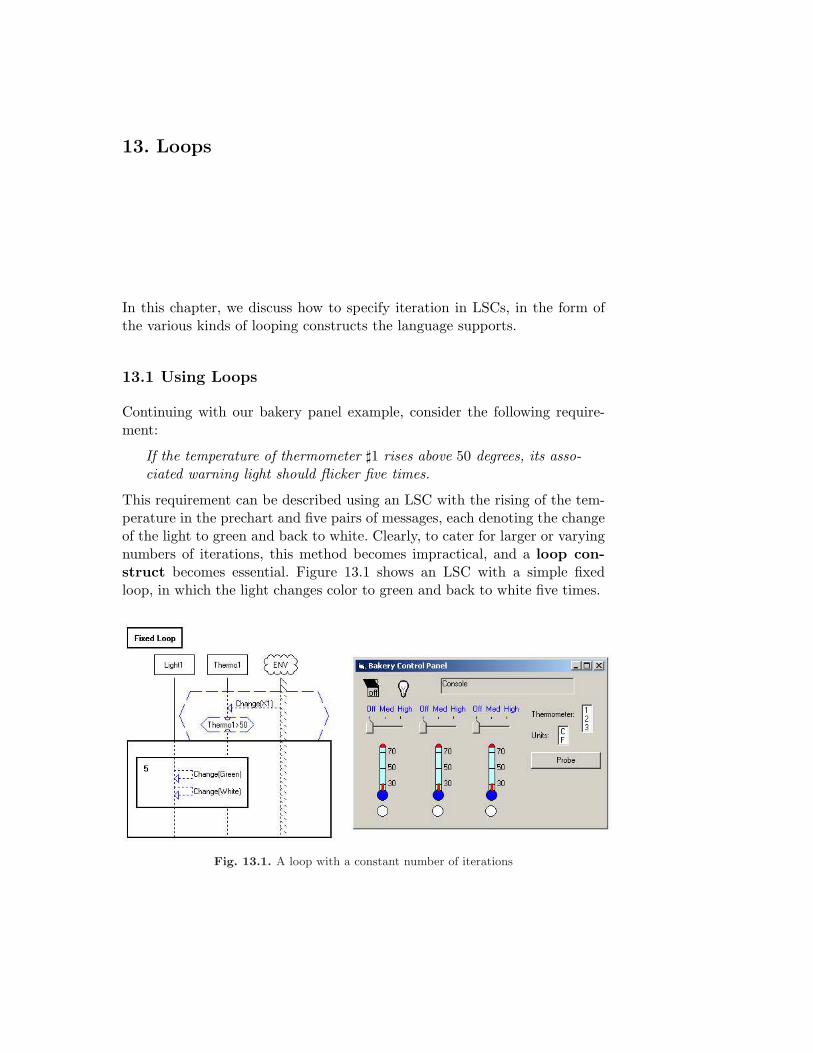
13. Loops
In this chapter, we discuss how to specify iteration in LSCs, in the form ofthe various kinds of looping constructs the language supports.
13.1 Using Loops
Continuing with our bakery panel example, consider the following require-ment:
If the temperature of thermometer ]1 rises above 50 degrees, its asso-ciated warning light should flicker five times.
This requirement can be described using an LSC with the rising of the tem-perature in the prechart and five pairs of messages, each denoting the changeof the light to green and back to white. Clearly, to cater for larger or varyingnumbers of iterations, this method becomes impractical, and a loop con-struct becomes essential. Figure 13.1 shows an LSC with a simple fixedloop, in which the light changes color to green and back to white five times.
Fig. 13.1. A loop with a constant number of iterations

176 13. Loops
Now, suppose we want the light to flicker as long as the temperatureremains above 50 degrees, rather than a fixed number of times. Here, thenumber of iterations is a priori unknown and depends on the dynamic be-havior of the system. Figure 13.2 shows an LSC for this, in which the loop isunbounded (denoted by a ‘*’). An unbounded loop iterates forever, and can
Fig. 13.2. An unbounded loop
be exited, like any other subchart, if a cold condition inside it evaluates tofalse. In this case, the loop will iterate and the light will keep flickering, aslong as the condition is true, i.e., until the temperature decreases to below50 degrees.
13.2 Playing In
Playing in loops is done in a way similar to that for if-then-else constructs.Here too, when the user wishes to play in a loop he/she clicks the loopicon on the toolbar and a loop wizard opens (see Fig. 13.3). As long as thewizard is open, the user can keep on playing in behavior as usual and allthe generated constructs (e.g., messages, assignments, etc.) are placed insidethe loop. When the user clicks End Loop, the loop is closed and the cursoris placed immediately after it. If elements are to be added inside the loopafter it is closed, the user can drag the cursor and drop it anywhere insidethe loop. The elements played in from that point on will be located insidethe loop, immediately prior to the cursor.
Figure 13.4 shows an example in which the loop is fixed but the numberof iterations is not given as a constant but is represented by a variable T . In

13.2 Playing In 177
Fig. 13.3. Playing in loops
Fig. 13.4. Using a variable as the number of iterations
play-out, the loop will iterate T times, where T is the number of the currentlyselected thermometer in the thermometer selector. Had T changed its valuewithin the loop body, this could not have changed the number of iterations,which is fixed in advance based on the value of T when the loop is started.
Three kinds of loops are defined in our extended language of LSCs. As wehave seen, a fixed loop is performed a fixed number of times, which can begiven as either a constant or as the value of a variable in the chart.
The second kind of loop is the unbounded loop we have seen, which isperformed an a priori unknown number of times and is exited only when acold condition in it evaluates to false. Note that placing a cold condition Cat the beginning or end of an unbounded loop creates a while C do or repeatuntil ¬C construct, respectively. One can also place a cold condition with aSELECT statement in the loop, thus specifying that it should be iterated anondeterministic number of times, governed by the probability given therein.

178 13. Loops
Having unbounded loops as part of the language is not only a matter ofconvenience, it increases the computational power of the language so thatin the presence of integer variables it can express the full range of recursivefunctions; bounded loops can express only primitive recursive ones.
The third kind of loop is the dynamic loop, annotated with a ‘?’, forwhich the user determines the number of iterations at run time.
13.3 Playing Out
During play-out, a loop can be entered, like any other subchart, only if allthe instances that participate in it have reached their locations at the loopstart. Before entering the loop, its maximal number of iterations is stored.If the loop is fixed, this number is known; if the loop is unbounded, themaximal number of iterations is set to infinity. If the loop is dynamic, theuser is prompted on the fly for the desired number of iterations (see Fig.13.5). The user specifies the desired number, and can also indicate whether
Fig. 13.5. Setting up a dynamic loop
he/she would like to be prompted again after that number of iterations isover. Dynamic loops are quite powerful when it comes to testing differentbehaviors of the system.
As the execution progresses and the loop is iterated, the Play-Engineprovides runtime information to help the user monitor the course of exe-cution. Figure 13.6 shows an example of such runtime information. In thetop-left corner of the loop subchart, the Play-Engine indicates that the loopis currently in its second iteration out of three (denoted by 2/3), and in thetop-right corner it shows the number of already completed iterations. The
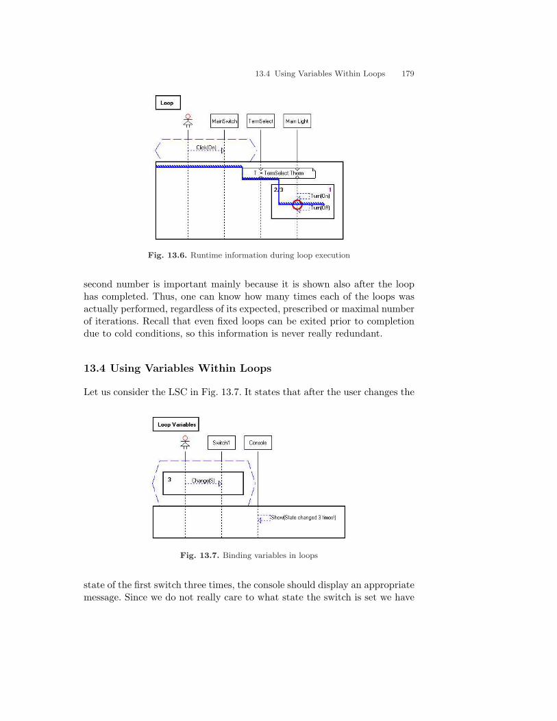
13.4 Using Variables Within Loops 179
Fig. 13.6. Runtime information during loop execution
second number is important mainly because it is shown also after the loophas completed. Thus, one can know how many times each of the loops wasactually performed, regardless of its expected, prescribed or maximal numberof iterations. Recall that even fixed loops can be exited prior to completiondue to cold conditions, so this information is never really redundant.
13.4 Using Variables Within Loops
Let us consider the LSC in Fig. 13.7. It states that after the user changes the
Fig. 13.7. Binding variables in loops
state of the first switch three times, the console should display an appropriatemessage. Since we do not really care to what state the switch is set we have

180 13. Loops
used a symbolic message with a variable S. But using a naive semantics hereis problematic: Recall that as the execution progresses, variables in symbolicmessages are bound to concrete values as a result of the various events beingcarried out. Suppose the user sets the first switch to High. As a result, a copyof this LSC is created, in which S is bound to High. If the user then changesthe state of the switch to Med, this event will not be unified with the messagein the LSC, since S is already bound to a different value. This is clearly notwhat we had in mind when playing in the LSC. And, indeed, we have chosena semantics different from the one just described for variables within loops.According to the proposed semantics, every time the loop body is re-entered,all the variables that occur for the first time inside the loop (in the sense ofSect. 7.2) are freed from their bindings, thus enabling rebinding with newvalues. This way, the LSC of Fig. 13.7 behaves exactly as desired.
We free only variables that occur for the first time inside the loop, sinceif the variable used in the loop is the same as one used prior to the loop, theintention is to restrict its value in the loop to the one it was bound to beforethe loop was started. Figure 13.8 shows a similar LSC, except that now S is
Fig. 13.8. Using an already bounded variable in a loop
bound outside the loop with the first state to which the switch is changed.In this case the two remaining occurrences can be unified only with eventsthat change the switch to the same state, which is quite different from themeaning the semantics assigns to the LSC of Fig. 13.7.

13.5 Executing and Monitoring Dynamic Loops 181
13.5 Executing and Monitoring Dynamic Loops
In this section we discuss some of the delicate aspects concerning the differ-ences between executing a loop in an LSC and monitoring it with respect toa given system run.
When it comes to fixed and unbounded loops, the mechanisms for exe-cuting and monitoring the loops are quite similar. In both cases, the loop isentered, and is iterated a fixed number of times, or until a false cold condi-tion is encountered. The main difference is that when it is executing an LSCspecification, the Play-Engine selects the events to be carried out, whereaswhen it is monitoring, the sequence of events is provided externally.
The major differences between executing and monitoring loops arise fordynamic loops. As explained, when a dynamic loop is encountered in a uni-versal chart, the user is prompted for the desired number of iterations. Thisis true not only for loops within the main chart but also in the prechart. Thismay be somewhat counterintuitive, since in the prechart the Play-Enginemonitors events and does not initiate them. So why can’t the Play-Enginemonitor a dynamic loop and determine on its own when the loop is over?Well, consider Fig. 13.9, in which, after the user flips the switch betweenon and off a number of times that is to be determined at runtime, the lightshould turn on. Suppose now that the user flips the switch to on and a copy
Fig. 13.9. A dynamic loop in the prechart
of this LSC is created. If the user now flips the switch to off, the Play-Enginefaces the following dilemma: Should it wait for the user to continue flippingthe switch or should it proceed to the main chart and initiate the event ofturning the light on? Since the Play-Engine cannot resolve this dilemma on

182 13. Loops
its own, the user is prompted for the number of iterations as soon as the loopis reached, even though we are in the prechart.
When a user is prompted for the number of iterations he/she may specify‘0’ to indicate that in the current run the loop should not be executed atall. In this case the loop is skipped and the Play-Engine continues executingthe events that follow it. There could be cases, like the one in Fig. 13.9,where the loop is reached only after one of its minimal events has alreadyoccurred (since it is a minimal visible event in the prechart). In such casesthe Play-Engine enters the loop and then prompts the user post factum forthe desired number of iterations. If the user chooses ‘0’, the chart is closedsince the prechart was violated.
In contrast to executing universal charts, when it monitors an LSC thePlay-Engine does not have to initiate execution of events at any point. Hence,dynamic loops can be used to further extend the expressive power of LSCsand to indicate sequences of events that repeat an a priori unknown number oftimes (including 0) but for which the number of iterations is not determinedby any constant, variable or condition. Figure 13.10 shows an example of anexistential LSC with two dynamic loops. This LSC can be activated either
Fig. 13.10. A dynamic loop in a monitored LSC
by the user changing the state of the first switch, in which case the first loopis entered, or by the user clicking the Probe button, in which case the firstloop is skipped, i.e., it is carried out 0 times. If the chart was started by theuser changing the state of the switch, the Play-Engine will keep monitoringthe incoming events and will exit the loop upon receiving the event of theprobe button being clicked. In the same spirit, two probe-clicks alone also

13.6 And a Bit More Formally ... 183
satisfy the chart, since both of the loops are carried out 0 times and the LSCcompletes.
Besides these differences between monitoring and executing dynamicloops, the Play-Engine is required to handle loop endings differently whenthey are executed and when they are monitored. During execution, when aloop reaches its end, the Play-Engine can immediately determine whether toexit the loop or return to its beginning. When monitoring dynamic loops,the Play-Engine waits before the loop end until the next event arrives. If theevent matches a minimal event in the body of the loop, the execution con-tinues from the loop’s start. If it matches an event that immediately followsthe loop, the loop is exited and execution continues from there.1
13.6 And a Bit More Formally ...
Following the semantics skeleton, we show the extensions and modificationsneeded to support the various kinds of loop constructs.
System Model and Events
Loop constructs are entirely specification oriented and therefore do not affectthe system model.
LSC Specification
An LSC L is extended to contain loop constructs as follows:
L = 〈IL, VL,ML, [PchL], AL, CL, SUBL, ITEL, LOOPL, evnt, subchart, temp〉
where LOOPL is the set of loops in L.A loop construct Loop in LOOPL is defined as:
Loop = 〈Kind, µ, Sub〉
where Kind ∈ {Fixed, Unbounded, Dynamic} is the loop’s kind, µ ∈ N ∪{∞} is the loop’s number of iterations, and Sub ∈ SUBL is the subchartcontaining the loop events to be iterated. We denote by ILoop = ISub the setof instances participating in the loop.
For the rest of this chapter, we use the term dynamic loops only for dy-namic loops that appear in monitored LSCs. Dynamic loops in executable1 If the event matches both a minimal event in the loop’s body and an event that follows
the loop, our implementation chooses to go back to the loop start.
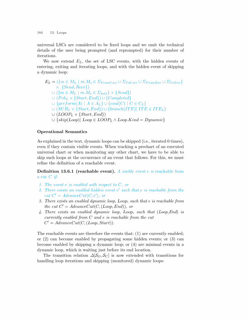
184 13. Loops
universal LSCs are considered to be fixed loops and we omit the technicaldetails of the user being prompted (and reprompted) for their number ofiterations.
We now extend EL, the set of LSC events, with the hidden events ofentering, exiting and iterating loops, and with the hidden event of skippinga dynamic loop:
EL = ({m ∈ ML | m.Ms ∈ ΣFromUser ∪ΣToUser ∪ΣFromEnv ∪ΣToEnv}× {Send, Recv})
∪ ({m ∈ ML | m.Ms ∈ ΣSelf} × {Send})∪ (PchL × {Start, End}) ∪ {Completed}∪ {perform(A) | A ∈ AL} ∪ {eval(C) | C ∈ CL}∪ (SUBL × {Start, End}) ∪ {branch(ITE)| ITE ∈ ITEL}∪ (LOOPL × {Start, End})∪ {skip(Loop)| Loop ∈ LOOPL ∧ Loop.Kind = Dynamic}
Operational Semantics
As explained in the text, dynamic loops can be skipped (i.e., iterated 0 times),even if they contain visible events. When tracking a prechart of an executeduniversal chart or when monitoring any other chart, we have to be able toskip such loops at the occurrence of an event that follows. For this, we mustrefine the definition of a reachable event.
Definition 13.6.1 (reachable event). A visible event e is reachable froma cut C if:
1. The event e is enabled with respect to C, or2. There exists an enabled hidden event e′ such that e is reachable from the
cut C ′ = AdvanceCut(C, e′), or3. There exists an enabled dynamic loop, Loop, such that e is reachable from
the cut C ′ = AdvanceCut(C, (Loop,End)), or4. There exists an enabled dynamic loop, Loop, such that (Loop,End) is
currently enabled from C and e is reachable from the cutC ′ = AdvanceCut(C, (Loop, Start)).
The reachable events are therefore the events that: (1) are currently enabled;or (2) can become enabled by propagating some hidden events; or (3) canbecome enabled by skipping a dynamic loop; or (4) are minimal events in adynamic loop, which is waiting just before its end location.
The transition relation ∆[SO,SC ] is now extended with transitions forhandling loop iterations and skipping (monitored) dynamic loops:

13.6 And a Bit More Formally ... 185
• If e = 〈M, t〉 (where t ∈ {Send, Recv}) then:1. Set Context ← ∅.2. If ∃CL ∈ SC and ∃e′ ∈ CL.LSC, such that e and e′ are nega-
tively level1-unifiable and e′ violates CL, then set SC ← SC \ {CL}.If temp(CL.Cut) = hot, set Violating ← True.
3. For every universal LSC L ∈ SO which has an event e′, positively level1-unifiable with e, as a minimal event in its prechart, create a copy ofL, CL, and set SC ← SC ∪ {CL}. Set CL.Mode = PreActive and setits cut by CL.Cut ← AdvanceCut(InitialCut(L), 〈PchL, Start〉). Unifythe variables of e and e′, by Unify(e, e′, Context). For each hidden evente′′ <L e′, apply ∆(e′′).
4. For every existential LSC L ∈ SO which has an event e′, positively level1-unifiable with e, as a minimal event in the chart body, create a copy ofL, CL, and set SC ← SC ∪{CL}. Set CL.Mode = Check, and set its cutto the beginning of the chart by CL.Cut ← BeginMainCut(CL.LSC).Unify the variables of e and e′, by Unify(e, e′, Context). For each hiddenevent e′′ <L e′, apply ∆(e′′).
5. For every copy CL ∈ SC which has a reachable event e′, positively level1-unifiable with e, set its cut by CL.Cut ← AdvanceCut(CL.Cut, e′).Then, if e′ = 〈M,Send〉, M is synchronous and e′′ = 〈M,Recv〉, setthe cut by CL.Cut ← AdvanceCut(CL.Cut, e′′). Unify the variables ofe and e′, by Unify(e, e′, Context). For each hidden event e′′ <L e′, apply∆(e′′).
• If e = Completed(CL) for some CL ∈ SC , then set SC ← SC \ {CL}.• If e = 〈PchL, End〉 for some CL ∈ SC , then set
CL.Cut ← BeginMainCut(CL.LSC) and CL.Mode ← Active.• If e = perform(A) for some A ∈ AL s.t. CL ∈ SC , then set CL.Cut ←
AdvanceCut(CL.Cut, e) and set
A.V ←
A.C if A.Type = constantV alue(A.P ) if A.Type = propertyA.f(A.λF
f ) if A.Type = function
• If e = eval(C) for some C ∈ CL s.t. CL ∈ SC then1. If value(C) = true then set CL.Cut ← AdvanceCut(CL.Cut, e).2. If value(C) = false then
a) If subchart(C) ∈ {ITE.SubT , ITE.SubE} for some ITE then
set CL.Cut ← AdvanceCut(CL.Cut, (ITE,End))
b) If subchart(C) = Sub ∈ SUBL then
set CL.Cut ← AdvanceCut(CL.Cut, (Sub, End))

186 13. Loops
c) If subchart(C) = ⊥ then set SC ← SC \ {CL}.d) If temp(C) = hot then set Violating ← True.
• If e = branch(ITE) for some ITE ∈ CL s.t. CL ∈ SC then1. If value(ITE.C) = true then set
CL.Cut ← AdvanceCut(CL.Cut, (ITE.SubT , Start)).2. If value(ITE.C) = false then
set CL.Cut ←{
AdvanceCut(CL.Cut, (ITE.SubE , Start)) if ITE.SubE 6= ⊥AdvanceCut(CL.Cut, (ITE.SubT , End)) if ITE.SubE = ⊥
• If e = (ITE.SubT , End) for some ITE ∈ CL s.t. CL ∈ SC then
set CL.Cut ← AdvanceCut(CL.Cut, (ITE,End))
• If e = (ITE.SubE , End) for some ITE ∈ CL s.t. CL ∈ SC then
set CL.Cut ← AdvanceCut(CL.Cut, (ITE.SubE , End))
• If e = (Sub, End) for some Sub ∈ CL s.t. CL ∈ SC then
set CL.Cut ← AdvanceCut(CL.Cut, (Sub, End))
• If e = skip(Loop) for some Loop ∈ CL s.t. CL ∈ SC then
set CL.Cut ← AdvanceCut(CL.Cut, (Loop,End))
• If e = (Loop, Start) for some Loop ∈ CL s.t. CL ∈ SC then
set CL.Cut ← AdvanceCut(CL.Cut, (Loop, Start))
For every variable V ∈ VL that is used in Loop for the first time, setV.ω ← ⊥.
• If e = (Loop, End) for some Loop ∈ CL s.t. CL ∈ SC and Loop.Kind 6=Dynamic then1. Set µ ← µ− 1.2. If µ > 0 then
set CL.Cut ← AdvanceCut(CL.Cut, (Loop, Start))
For every variable V ∈ VL that is used in Loop for the first time, setV.ω ← ⊥.
3. If µ = 0 then
set CL.Cut ← AdvanceCut(CL.Cut, (Loop,End))

13.7 Bibliographic Notes 187
Since the events of entering, exiting and iterating loops are additionalforms of hidden events, the procedures step and super-step handle them withno modifications. The procedure monitor-event has to be modified so that itdoes not propagate the hidden event of ending a dynamic loop, but ratherleaves the cut positioned just prior to the loop end in order to be able toaccept events that appear after the loop start as well as ones that appearafter the loop end.
monitor-event(ev)
1. Apply ∆[SM ,ML](ev).2. Compute the set of enabled events:
Enabled ←⋃
CL∈ML{e ∈ EL | enabled(e)}
Waiting ←⋃
CL∈ML{e | e = branch(ITE)}
∪⋃
CL∈ML{e | e = (Loop,End) ∧ Loop.Kind = Dynamic}
Enabled ← Enabled \Waiting
3. If there is a hidden enabled event e ∈ Enabled, thena) Apply ∆[SM ,ML](e).b) Go back to 2.
4. Terminate monitor-event.
13.7 Bibliographic Notes
The original definition of the MSC standard [123] allows the specification ofrepeated interactions by means of a loop expression. The number of possi-ble repetitions can be constrained by upper and lower bounds. Setting bothbounds to be the same causes the loop to iterate an exact number of times,and setting the upper bound to infinity yields an unbounded loop. The num-ber of iterations of fixed loops in MSCs can be specified with a constant onlyand not with a variable. Since conditions are not given a precise semanticswith regard to the scope they are defined in, they cannot be used in MSCsto construct ‘while-do’ and ‘repeat-until’ constructs.
If an MSC contains a loop with proper upper and lower bounds, meaningthat the former is larger than the latter, a system would satisfy this MSConly if the loop is iterated for a number of times that is in the specifiedrange. However, the MSC standard does not say anything about the number

188 13. Loops
of iterations that such a loop should be performed had we wished to take anexecutable approach like the one we have for LSCs. This is fine for MSCs,since they are oriented towards testing, but it is not enough for LSCs, whichhave to be executable.
As discussed in the bibliographic notes for Chap. 10, the MSC standardalso describes a higher-level way of connecting MSCs, hierarchical MSCs(HMSCs). The underlying graph of an HMSC may contain cycles, thus al-lowing for the specification of loops, which are repeated sequences of bMSCs(basic MSCs). As is the case with subcharts, a major difference between aloop in an LSC and in an HMSC lies in the synchronization requirement. InLSCs, all the instances that participate in a loop synchronize at the beginningand end of the loop, while in HMSCs there is no such requirement. It hasbeen observed in several papers, e.g., [10], that allowing processes to progressalong the HMSC with each object being in a different node may introduceirregular behavior, and is the cause of undecidability of certain properties.Undecidability results and ways to restrict HMSCs in order to avoid suchproblems can be found in [9, 40, 57, 56].

14. Transition to Design
So far, we have seen how the play-in/play-out approach and its implemen-tation in the Play-Engine help in the process of capturing and validatingscenario-based behavioral requirements. As we have seen, the graphical userinterface of the system is used extensively in both play-in and play-out. Inthe former the GUI objects are used to specify user actions and system re-actions, and in the latter they are used to reflect the system reactions as thespecification is executed, and to allow the user to input external events. Wehave also seen how existential LSCs can be used to specify system tests andhow they can be monitored in the Play-Engine for successful completion. Ifwe indeed want to think of our methodology and tool as being useful not onlyfor requirements but also for specifying the system’s actual implementablebehavior, we have to talk about making a smooth transition from the require-ments phase into the design phase. This chapter is devoted to discussing someof the issues raised by this possibility.
14.1 The Design Phase
In many development methodologies, the design phase begins with a require-ments specification, usually given as a text document, following which sce-narios are constructed (say, in some variant of sequence diagrams) to showthe interaction between the objects comprising the system. The scenarios areconsidered to be an initial step towards formalizing the requirements. Usingplay-in and play-out, the designer is given a head start: He/she can beginthe design phase with the requirements specification already given as a setof executed and debugged LSCs, describing the allowed, necessary and for-bidden interactions between the system and its users and environment. Thisspecification is thus highly suitable as a basis for the design phase.
Beginning with this LSC specification, we can imagine the design phaseas consisting of the following activities, which would typically be carried outas part of an incremental and iterative (possibly spiral-like) process:

190 14. Transition to Design
• Identifying ‘internal’ objects (i.e., objects that are not represented in theGUI of the system) and their properties. This activity is usually affectednot only by the original behavioral requirements but also by other con-siderations, such as non-functional constraints, robustness of the design,design patterns, etc.
• Adding properties (e.g., state variables) to existing objects, both graphicaland internal.
• Describing the interactions between the objects comprising the system inincreasing levels of detail. To do this, the designer identifies the methodsof each object, through which it can be called, and the parameters to bepassed when invoking each of them. Then, existing LSCs and newly createdones are refined with method calls, interleaved with the original propertychanges of the objects. These method calls are used to show the controlflow that triggers the changes in the various values of the properties.
• Refining objects into sets of sub-objects and composing (clustering) sets ofobjects into compound objects. During these processes, we allow the useof appropriate levels of detail in the inter-object scenarios, and preservethe meanings of these scenarios under the refinement and composition ofobjects.
• Constantly making sure that the design is consistent with the original re-quirements. This is usually done by maintaining some kind of traceabilitybetween the requirements and the design.
The following sections show how the play-in/play-out approach and thePlay-Engine are extended to support most of these aspects in the transitionfrom requirements to design. We do note, however, that although the issue ofobject refinement and composition is extremely important, we have not yetworked it into our methodology and implementation. This is one of the maintopics for our future work; see Chap. 21.
14.2 Incorporating Internal Objects
Figure 14.1 shows a simple LSC stating that each time the user changesthe state of the switch, the light should change its state accordingly. In therequirements analysis phase, one does not have (and usually does not wish)to be more specific than this. However, it is clear that the way the LSC iscurrently specified, we do not know how the light is notified about the useraction and how it decides to turn on or off.
Let us assume that as a first step towards the design the user decides thatthe communication between the switch and the light will be carried via anew internal object — a controller. The Play-Engine allows the addition of

14.2 Incorporating Internal Objects 191
Fig. 14.1. High-level requirements
internal (i.e., GUI-less) objects on the fly. After creating an internal object,the user may specify properties for this object using an appropriate dialog.See Fig. 14.2. The user may specify a name for the newly created object (in
Fig. 14.2. Dialog for defining application objects
this case ‘Controller’) and define new properties for it. The bottom sectionof the dialog, termed ‘Methods’, is discussed in the next section.
After filling in all the details and closing the dialog, the object is addedto the set of application objects and can be used in the LSCs and duringplay-in and play-out. Figure 14.3 states that after the switch is flipped, theinformation is first transferred to the controller, which sets its state propertyto be the same as the switch, and only then does it reach the light. Note thateven the LSC of Fig. 14.3 does not specify how the information is passedbetween the objects, but only that it reaches an intermediate object that isresponsible for forwarding it to the light.

192 14. Transition to Design
Fig. 14.3. Using an internal object in an LSC
One point needs to be addressed here: if an internal object is not repre-sented in the GUI, how can it be used in playing in and playing out? Wehave decided to visually represent internal objects in a way similar to howthey are represented in most object-oriented methodologies and tools — byobject model diagrams. After an internal object is created, it is added tothe Play-Engine’s object map. The object map is a variant of an objectmodel diagram, which contains all the internal objects. For each object,the object map displays its sets of properties (see Fig. 14.4). Properties of
Fig. 14.4. Visualizing internal objects in an object map
internal objects are like properties of GUI objects, and are used to reflectvarious attributes of the objects. Since property values of internal objectscannot be visually reflected, as they can for graphical properties of GUI ob-jects, the value of each property is written next to the property name in theobject map, thus enabling the user to view the system state at a glance.

14.3 Calling Object Methods 193
Since the process of transition into design may entail adding new proper-ties to existing GUI objects, as well as to internal objects, the Play-Engineallows the addition of properties to GUI objects too. But since new proper-ties of GUI objects are not known to the GUI application, they cannot bevisually rendered in the GUI itself. To examine the current values of suchproperties, the user right-clicks an object and selects Properties from thepopup menu. In response, the Play-Engine displays a list of all the object’sproperties together with their current values.
14.3 Calling Object Methods
Continuing with our example, suppose that the user now wishes to specifyhow the information is transferred from the switch that was clicked by theuser, via the newly added controller, to the light, so it can change its state.We do this by adding methods to every object that needs to be called, andthen calling these methods to transfer the desired information.
Methods are means for transferring data or control signals between ob-jects. Each object can have an arbitrary number of methods, which otherobjects can call in order to transfer the required information. Every methodhas a name and a set of parameters defined over the application types. Amethod can be either synchronous or asynchronous, thus specifying whetherthe calling and the called objects synchronize when the method is called. Thelist of methods is shown both in the object dialog (as seen in the bottom sec-tion of the dialog in Fig. 14.2) and in the bottom part of the object rectanglein the object map (as seen in Fig. 14.4).
In our example, we add two identical methods SetState(S), with S rangingover {On,Off }, one to the controller and one to the light. We then move intoplay-in mode and play in a call from the switch to the controller. Figure 14.5shows the basic steps in playing in such interactions. The user first right-clicksthe switch and selects Call Other Object (see Fig. 14.5(a)). As a result, theswitch is highlighted and a tooltip appears above it showing “From” (see (b)).Next, the user right-clicks the target object. The Play-Engine knows that theuser is currently in the process of specifying a method call, and therefore theopened popup menu contains a list of all the methods of the target object(see (b)). After one of the methods is selected, a dialog opens up, in whichthe user instantiates the parameters of the method with concrete values orwith variables from the LSC (see (c)). When this process is over, a messagegoing from the caller object to the called object is added to the LSC (see(d)).

194 14. Transition to Design
Fig. 14.5. Playing in interactions with internal objects
Repeating this process, but with the controller as the source and the lightas the target, completes the desired interaction, resulting in the LSC of Fig.14.6.
Fig. 14.6. From the Switch to the Light via the Controller

14.3 Calling Object Methods 195
Adding this control flow information to a chart that initially contains onlyrequirements-level interaction between the system and its environment helpsfill the gap between what the system should do and how it does it. In ourexample, the ‘what’ part is given in the initial LSC, stating that the lightshould reflect the state of the switch, and the ‘how’ part is given in the fi-nal LSC by the interactions between the objects, which are interleaved withthose appearing in the original scenario. These interactions show how seem-ingly unrelated events become related, by explicitly showing the sequence (orsequences) of events that can lead from one to the other.
As discussed at the beginning of the chapter, by starting with LSCs cre-ated by, or on behalf of, the user, developers can achieve direct traceabilitybetween the behavioral requirements and the design. Although the determi-nation of internal objects, their properties and their methods can be affectedby various considerations other than the behavioral requirements, these ob-jects and properties should be integrated into the system in a way that sat-isfies the requirements that caused their addition but does not violate anyother requirements. After internal objects are added and the interaction be-tween objects is played in, the user may play out various scenarios and verifythat the system still behaves as expected.
In addition to all of this, continuous consistency between the requirementsand the design, as it evolves, can be checked using existential LSCs. Supposethat after the initial LSC of Fig. 14.1 is developed, a corresponding testis formulated, as shown in the existential LSC of Fig. 14.7. This LSC can
Fig. 14.7. Regression testing with existential LSCs
then be checked for satisfiability by clicking the switch to on and then tooff, and verifying that the two hot conditions evaluate to true when theyare reached. By leaving the existential chart unmodified, the designer mayprove the correctness of the modified universal LSC (i.e., the one in Fig. 14.6)

196 14. Transition to Design
by repeating the same sequence of actions and showing that this sequencesatisfies the test described by the existential LSC.
As shown in Chap. 12, a comprehensive set of system tests can be formu-lated as a set of existential LSCs. In the requirements phase, this set can bechecked for satisfiability, and for each test a satisfying run should be recorded.At any point during the design phase this set can then be used for regres-sion testing of the requirements, as follows. Each recorded run is modified tocontain only external events (i.e., events that were generated by the user orthe environment). These runs are then replayed, but with the new universalcharts now driving the execution, and the original existential charts beingmonitored. Since the existential tests do not (and for this purpose, indeedshould not) specify how the results are achieved but only that they are indeedeventually achieved, the new sequences of events generated by the modifieduniversal LSCs should still satisfy the tests.
Another way of performing regression testing to check for consistencybetween the original LSCs — those on the requirements level — and themodified, design-level LSCs would be to keep copies of the original LSCs andthen to simply execute the system, with both the old and the new LSCsdriving the execution. Figure 14.8 shows the initial and the final LSCs of ourexample being executed simultaneously.
Fig. 14.8. Consistency between requirements and design
14.4 Playing Out
Messages representing method calls can be symbolic (just like the usualkind of message). To support their execution, our unification algorithm isextended, so that messages that are sent between the same two objects, and

14.4 Playing Out 197
which represent the same method, can be unified if all their variables can bepairwise unified.
When LSCs containing method calls are played out, the Play-Engine high-lights the involved objects and animates the interaction by drawing arrowsbetween them. Thus, the play-out mechanism does not only let end-usersvalidate requirements but can also be used beneficially for demonstrating,reviewing and debugging a design. Figure 14.9 shows how the interactionbetween objects is animated during play-out. Note that the arrows are notlimited to being within the GUI application or the object map, but can runfrom one to the other. Send events are animated by arrows that start out with
Fig. 14.9. Animating interactions between objects
a solid line (the sender) and end up with a dashed line (the receiver), whilereceive events will be drawn the other way around. Synchronous messagesare shown as full solid arrows.

198 14. Transition to Design
14.5 External Objects
Often, a reactive system works in the presence of other elements, besidesthe user who interacts with it. These might include other systems, compo-nents, machines, computers, sensors, and even other humans or elements fromnature. The collection of all these elements is referred to as the system’s en-vironment. When playing in the required behavior of a reactive system, it isnecessary to be able to express its interaction with this environment. As wehave already seen, the Play-Engine allows the user to specify how the envi-ronment interacts with the system in a way similar to the interaction withthe end-user. However, such interactions with the environment are limited tochanges in object properties, and are thus suited to interactions with nature(e.g., the external temperature rising, devices breaking down, etc.), but lessso to true communication with interfacing systems (e.g., receiving data orcontrol signals).
The need to describe interactions with interfacing systems usually arisesalready in the requirements analysis phase, although there are cases wherethese aspects of the system may be ignored. For example, when specifyingthe behavioral requirements of a communication-guided missile, chances arethat we cannot ignore the control signals received from the guiding controlunit. In contrast, when specifying the requirements of an automatic tellermachine (ATM), we could probably describe the ATM as an integral system,and describe the communication with the remote bank server at a later phase.
When it comes to design, it is often the case that the design of a sys-tem is carried out by more than one person, each responsible for a set ofcomponents. In such cases, every designer in the team is aware of the en-tire behavioral specification, but is allowed to refine the specification of onlythose components for which he/she is responsible, and must do so in a waythat guarantees that they fit in correctly within the overall system behavior.While performing such a design task it is convenient for each team memberto refer to the objects under his/her responsibility as internal, and to theother objects, with which these are to interact, as external. As we shall seenext, the distinction between internal and external objects is not merely amatter of convenience, but is also reflected in the executable semantics of thelanguage.
To support the aforementioned design tasks within the language of LSCsand the play-in/play-out approach, we first extend the LSC language withthe ability to refer to external objects. Technically, within the Play-Engine,external objects are implemented as internal objects, i.e., non-GUI ones, andare distinguished from the usual internal objects by their external flag beingset to true.

14.5 External Objects 199
Having external objects within the specification entails more than justpartitioning the external environment into its components and giving themnames. In contrast to the external environment discussed in Chap. 5, exter-nal objects are not limited to changing property values of internal objects.External objects can have properties of their own, indicating their being indifferent states (e.g., active, ready for communication, etc.). They can alsocall system objects and be called by them, thus modeling the interaction withexternal systems.
Figure 14.10 shows an LSC, in which the switch instance represents anexternal object, and is therefore annotated with a small cloud.
Fig. 14.10. External objects in LSCs
When playing out scenarios and testing the system’s behavior, we wouldlike to be able to control the behavior of external objects, much like wecontrol the actions of the user and the external environment. As an example,consider the LSC in Fig. 14.11, which describes a simple interaction betweentwo interfaces. Suppose that we are given the task of creating a detaileddesign for Interface 2. For simplicity, assume that this entails adding a singleimplementation object, Impl 2, and a simple interaction with it. The detaileddesign is given in the LSC of Fig. 14.12. Note that the interfacing objectInterface 1 is now considered external.
To check our design, we would now like to use the play-out techniques inthe standard way. Recall, however, that property changes of internal objectsand method calls between objects are not carried out by the user; rather, theyare performed by the Play-Engine as part of its super-steps. In our example,we would like to activate the prechart of ‘Detailed Design’ by initiating thecall from Interface 1 to Interface 2. If the actions of Interface 1 were depen-dent upon the values of its properties, we would have also liked to be able tochange these values, and thus control the behavior of this object.

200 14. Transition to Design
Fig. 14.11. High-level interaction between interfaces
Fig. 14.12. Detailed design of Interface 2
To support this, the execution mechanism of the Play-Engine is modi-fied so that it does not initiate events that originate from external objects,much as it does not initiate events from the user or the external environ-ment. While playing out, the user can change property values of external

14.6 And a Bit More Formally ... 201
objects and can initiate calls from external objects to objects that are inter-nal to the system. Thus, it is the user who controls the behavior of externalcomponents and systems while the system under development is being ex-ecuted and analyzed. This extension to the play-out mechanism provides away for validating component-based requirements and designs, by allowingthe independent execution of each part and then combining the LSCs in thevarious parts into a fully integrated requirements or design specification. Sec-tion 21.5 in our Future Work chapter describes our work on linking severalPlay-Engines together, and is particularly relevant to the above discussion.
14.6 And a Bit More Formally ...
Following the semantics skeleton, we show the extensions and modificationsneeded to support method calls, and internal and external objects.
System Model and Events
The system model is extended to include method calls and to distinguishbetween internal and external objects.
A method with n formal parameters is defined as:
Method = Name(D1, D2, . . . , Dn)
where Name is the method name and Di ∈ D is the type of its ith parameter.A class is modified to have a set of methods, through which its object
instances can be called:
C = 〈Name,P,M〉
Next, an object can be declared as external:
O = 〈Name, C,PV, External〉
where External is a Boolean flag, set to true in external objects and to falsein all other objects.
We now redefine a system message Ms to also contain method informationif it represents a method call:
Ms = 〈Src,Dst, P, V, f, λFf , m, λM
m , Symbolic〉
where m ∈M∪ {⊥} is the method represented by the message and λMm is a
method information structure for m, defined as follows:

202 14. Transition to Design
λMm =
{(V1 ∈ m.D1, . . . , Vn ∈ m.Dn) if m ∈M⊥ if m = ⊥
If the message represents a method call m ∈M, then λMm contains variables
as actual parameters that replace the method’s formal parameters. If Ms doesnot represent a method call, then λM
m = ⊥. We require that each messagerepresent either a property change or a method call:
∀Ms : (Ms.P 6= ⊥)⊕ (Ms.m 6= ⊥)
Since method calls can also be synchronous and asynchronous, the defini-tion of synchronous messages is modified to reflect this.
Definition 14.6.1 (synchronous system messages). A message Ms issynchronous if Ms.P 6= ⊥ ∧Ms.P.Sync = true or Ms.m 6= ⊥ ∧Ms.m.Sync =true. A self message is also synchronous.
The alphabet of possible messages of Sys is extended to include messagesgoing between objects within the system and not only between objects andthe environment:
Σ = ΣFromUser ∪ΣToUser ∪ΣFromEnv ∪ΣToEnv ∪ΣSelf ∪ΣCalls
ΣFromUser = {Ms | Src = User ∧ P ∈ class(Dst).P}ΣToUser = {Ms | Dst = User ∧ P ∈ class(Src).P ∧ P.Affects = User ∧
P.InOnly = False}ΣFromEnv = {Ms | Src = Env ∧ P ∈ class(Dst).P ∧ P.ExtChg = True ∧
P.InOnly = False}ΣToEnv = {Ms | Dst = Env ∧ P ∈ class(Src).P ∧ P.Affects = Env ∧
P.InOnly = False}ΣSelf = {Ms | Dst = Src ∧ P ∈ class(Src).P ∧ P.Affects = Self ∧
P.InOnly = False}ΣCalls = {Ms | Dst, Src ∈ O ∧ m ∈ class(Dst).M}
The set of system events, E , is extended accordingly:
E = ((ΣFromUser ∪ΣToUser ∪ΣFromEnv ∪ΣToEnv ∪ΣCalls)× {Send, Recv})∪ (ΣSelf × {Send})
LSC Specification
The set of LSC events is extended to contain messages that represent inter-actions between system objects:

14.6 And a Bit More Formally ... 203
EL =({m ∈ ML | m.Ms ∈ ΣFromUser ∪ΣToUser ∪ΣFromEnv ∪ΣToEnv ∪ΣCalls}× {Send, Recv})
∪ ({m ∈ ML | m.Ms ∈ ΣSelf} × {Send})∪ (PchL × {Start, End}) ∪ {Completed}∪ {perform(A) | A ∈ AL} ∪ {eval(C) | C ∈ CL}∪ (SUBL × {Start, End}) ∪ {branch(ITE)| ITE ∈ ITEL}∪ (LOOPL × {Start, End})∪ {skip(Loop)| Loop ∈ LOOPL ∧ Loop.Kind = Dynamic}
The notion of a message affecting a variable is extended. Now, an LSCmessage M ∈ ML affects a variable X also if the variable is used as a param-eter in a method call.
Definition 14.6.2 (affecting a variable). An LSC message M ∈ ML af-fects a variable X, if M.Ms.V = X or X ∈ M.Ms.λ
Mm . An assignment
A ∈ AL affects a variable X if A.V = X.
Operational Semantics
The operational semantics is changed in two ways. First, the notion of mes-sage unification is extended to support method calls. Then, the set of externalevents is extended to include send events that originate from external objects,so that these events will not be candidates for execution in the proceduresuper-step.
We now extend the notion of unification to apply also to method calls,so that two method information structures are unifiable if they represent thesame method and their variables are pairwise unifiable.
Definition 14.6.3 (method unification). Two method information struc-tures λM
m1and λM
m2are Q-unifiable (where Q is ‘positively’ or ‘negatively’) if:
m1 = m2
∧ ∀i : λMm1
.Vi and λMm2
.Vi are Q-unifiable.
The message content Λ of a message Ms is modified to refer to methodswhen relevant.
Definition 14.6.4 (message content).
Ms.Λ =
Ms.λFf if λF
f 6= ⊥Ms.λ
Mm if λM
m 6= ⊥Ms.V otherwise

204 14. Transition to Design
Definition 14.6.5 (message unification). Two system messagesMs = 〈Src, Dst, P, V, f, λF
f , m, λMm , Symbolic〉 and
M ′s = 〈Src′, Dst′, P ′, V ′, f ′, λF
f ′ , m′, λM
m′ , Symbolic′〉 are Q-unifiable (whereQ is ‘positively’ or ‘negatively’) if Src = Src′, Dst = Dst′, P = P ′, m = m′
and their contents are Q-unifiable.
Since message variables may bind to values as a result of unifying differentmethod information structures during execution, we add another unificationprocedure to handle such cases:
Unify(λMm , λM
m′, Context)
1. For i = 1, . . . , n:a) Unify(λM
m .Vi, λMm′.Vi, Context)
Having these definitions, the transition relation ∆ supports method callswith no modifications. In Chap. 5, we defined the set of external events assend events that are initiated by the user or the environment:
External = {⋃
L∈S〈m,Send〉 | m.Ms.Src ∈ {User,Env}}
We now modify this definition to include send events from all external objects.For brevity, we will refer to User and Env as external objects and will nottreat them separately:
External = {⋃
L∈S〈m,Send〉 | m.Ms.Src.External = true}
Having modified the set of external events, the procedure super-step remainsunchanged.

14.7 Bibliographic Notes 205
14.7 Bibliographic Notes
Constructing a program from a requirements specification is the long-knowngeneral and fundamental synthesis problem. This chapter was devoted todiscussing briefly a methodology, supported by the Play-Engine tool, for re-fining a set of requirements given as LSCs into a design also given as anLSC specification. Since we use the same language and the same pattern ofthought for both phases, the synthesis problem becomes a lot easier. In thedevelopment scheme outlined in [43], an important facet is the ability to syn-thesize an intra-object implementation from the inter-object requirements.This is a whole lot harder than our LSC-to-LSC process, or the problem ofgenerating lower-level code from an already intra-object system model (whichis really but a high-level kind of compilation). The duality between the inter-object scenario style for requirements and the intra-object statechart stylefor design renders useful synthesis a truly difficult task.
There has been a lot of work on the limited case of state-machine synthesisfrom variants of classical message sequence charts. This problem is a lot easierthan synthesis from LSCs, since MSCs do not enable expressing forbidden ormandatory behavior, so there is very little in the way of real constraints onbehavior. Also, some of the synthesis papers do not even allow the systemto be simultaneously in different charts, and so really relate to a single chartonly. Work on synthesis from MSCs includes the SCED method [66, 67, 68],based on the algorithm of [15], and synthesis in the framework of ROOMcharts [77]. Other relevant work appears in [108, 10, 18, 72]. New efforts onsynthesis appear in [5, 119].
A lot of work has also been carried out on synthesizing state-based sys-tems from requirements given in temporal logic. Due to the expressivepower of temporal logic, this problem is closely related to synthesizing fromLSCs. The early work on such synthesis considered closed systems that donot interact with the environment [83, 34]. In this case, a program can beextracted from a constructive proof that the formula is satisfiable. This ap-proach is not suitable for synthesizing open systems that interact with theenvironment, since satisfiability implies the existence of an environment inwhich the program satisfies the formula but the synthesized program cannotrestrict the environment. Later work in [98, 96, 1, 121] dealt with the synthe-sis of open systems from linear temporal logic specifications. The realizabilityproblem is reduced to checking the non-emptiness of tree automata, and afinite state program can be synthesized from an infinite tree accepted by theautomaton. The problems of realizability checking and synthesis from lineartemporal logic have been shown to be 2EXPTIME-complete. Work on syn-thesis from branching temporal logics, based on alternating tree automata

206 14. Transition to Design
[73], show that the synthesis problems for CTL and CTL∗ are EXPTIMEand 2EXPTIME complete, respectively. In [97] synthesis of a distributed re-active system is considered. Given an architecture — a set of processors andtheir interconnection scheme — a solution to the synthesis problem yieldsfinite state programs, one for each processor, whose joint behavior satisfiesthe specification. It is shown in [97] that the realizability of a given specifi-cation over a given architecture is undecidable. Previous work assumed theeasy architecture of a single processor, and then realizability was decidable.
Turning to LSCs, there is the work described in [65], which synthesizesa timed Buchi automaton from a single LSC (and code can then be derivedfrom the automaton). A more general approach appears in [46], where thesynthesis problem for a multiple-chart LSC specification is tackled by firstdefining consistency, then showing that an LSC specification is consistent iffit is satisfiable by a state-based object system, and finally synthesizing a sat-isfying system as a collection of finite state machines or statecharts. A globalautomaton for the entire system is constructed, which is then distributed be-tween the objects in the system. Construction of the global automaton in [46]causes a state explosion problem, which must be tackled somehow in order forthe algorithm to become practical. Also, the LSCs in [46] are restricted: forexample, conditions are excluded and specific restrictions on the interactionof the environment with the system are assumed.
Another approach that tries to bridge the gap between requirements anddesign by using a common representation for both is called genetic softwareengineering (GSE) [33], in which a requirement written in natural languageis formalized by a ‘behavior tree’. All such trees are then integrated intoa single tree. This comprehensive system behavior tree is transformed bya variety of manipulations and projections into a components architecturediagram, and then into many component trees, each describing the internalbehavior of a single component. GSE is also similar to our approach in that ituses a richer specification language than conventional sequence charts (e.g.,it can specify anti-scenarios).
The software cost reduction (SCR) method described in [55] also allowsthe specification and simulation of requirements for reactive systems. TheSCR method provides a tabular notation for specifying the required rela-tion between system and environment variables and also uses a GUI in thefinal phase of simulation. According to this method, requirements are firstdescribed using nondeterministic and possibly incomplete relations betweenvariables, and then the specification is modified, with the aid of an auto-mated tool, to be deterministic and can then be simulated. The process ofrefining the requirements and making them deterministic can also be viewedas a kind of design. SCR is different from our work in the languages used

14.7 Bibliographic Notes 207
(i.e., tables of variables vs. visual notations) and in the requirement that thefinal model should be deterministic.
A methodology supported by a tool called LTSA for specifying and ana-lyzing labeled transition systems (LTSs) is presented in [81, 114]. This toolworks with an animation framework called SceneBeans [99], yielding a nicelyanimated executable model. The model has to be an LTS, which is moreakin to the intra-object statecharts than to inter-object sequence based be-havior, and it will usually be larger and more detailed than sequence charts.The behavior can be either written in FSP [80] and compiled into LTSs, ordescribed as MSCs and transformed using a synthesis algorithm into LTSs[114]. An interesting idea would be to use SceneBeans as an animation engineto describe the behavior of internal (non-GUI) objects in our Play-Engine.


15. Classes and Symbolic Instances
In Chap. 7 we showed how scenarios can be generalized using symbolic mes-sages. Symbolic messages are but one aspect of defining generic scenarios —the simpler one. This chapter addresses symbolic object instances, which isthe more complicated and more powerful aspect of genericity.
Many systems feature multiple objects that are instances of the sameclass, which is one of the central maxims of the object-oriented paradigm. Forexample, a communication system contains many phones, and a railroad con-trol system has many trains and terminals and possibly also many distributedcontrollers. We would like to be able to specify inter-object scenario-basedbehavior in a general way, on the level of classes and their parameterizedinstances, not necessarily restricting them to concrete objects. Not surpris-ingly, the issue of executing such behavior is quite subtle, since figuring outexactly what is going on, and in which objects, must be continuously done onthe fly. In this chapter, we extend the LSC language with symbolic instancesand discuss playing in and playing out the resulting specifications, includingthe delicate semantic issues that arise.
15.1 Symbolic Instances
Consider a telephone network consisting of four phones, one central switch-board and four channels, each connecting one phone to the switch. Figure15.1 shows a graphical user interface for this system. Now, suppose we wouldlike to say that for every phone, when the ‘C’ button is clicked, the displayshould be cleared. Figure 15.2 shows an LSC describing this requirement forPhone1. To specify the same requirement for the other telephones, the LSCshould be replicated for each phone. This may become very inconvenient andinefficient when the number of phones is large, and may also become impos-sible in systems where the number of phones is unknown (dynamic creationand destruction of objects) or in parameterized systems where the numberof phones is fixed, but is given as a parameter.
To solve these problems and to enable the creation of more compact LSCspecifications, we introduce symbolic instances. Recall that every object

210 15. Classes and Symbolic Instances
Fig. 15.1. NetPhone: the GUI for a telephone network
Fig. 15.2. A concrete scenario for clearing a display
in our system model is an instance of some specific class. A symbolic instancerepresents an entire class rather than one concrete object, and can bind toconcrete objects at runtime. Figure 15.3 shows an LSC where one of theinstances is symbolic and represents the class Phone (denoted by ‘Phone::’).The chart states that its scenario should hold for every actual phone of classPhone in the system, regardless of the number of actual phones and whetherthese phones are static or were created dynamically during the system run.
15.2 Classes and Objects
Before we get into the more complex features of symbolic instances, let usspend some time on how classes and objects show up in the play-in/play-out methodology. Classes in object-orientation are used to describe sets ofobjects that share a common behavior. The objects themselves are commonlyreferred to as the class instances. Classes are usually introduced in the design

15.2 Classes and Objects 211
Fig. 15.3. A generalized scenario for clearing the display of any phone
phase, where the behavior of each class is given in an intra-object style, say,using a statechart or code, thus describing how each of the objects in theclass behaves under different circumstances.
In the play-in/play-out approach, we are not interested in how each of theobjects behaves as an independent entity, but, rather, in how a set of objectsinteracts in an inter-object style to satisfy certain desired (or undesired) sce-narios. Therefore, classes in our approach serve more as interfaces, i.e., asplace holders for sets of objects that are interchangeable in the specified sce-narios. Put another way, classes are not used to describe the overall commonbehavior of sets of concrete objects, but, more operationally, to specify thatin certain scenarios any concrete object from the set of class instances canbe used, and that the scenario should still hold (or that a forbidden scenariois not allowed to hold for any instance of the class).
The Play-Engine provides several ways to create classes and objects andto associate them with others. A class can be created from scratch, or can bebased on an already existing object. In the former case, the user names theclass and specifies the class properties and methods. In the latter case, theclass properties and methods are derived from those of the object on whichthe class is based. Creating classes based on existing objects is very usefulin cases where the GUI application comes with sets of similar objects, andone would like to handle them in identical ways. Note that a class is notrestricted to have either GUI objects as instances or internal objects, butmay contain instances of both kinds. For example, in our telephone system,we could create a ‘backup’ switch as an internal object and then let both theGUI switch and the internal switch be instances of a Switch class.
An alternative way to associate objects with classes is to start with a classand then create objects based on that class. After creating some classes, theconcrete objects may be associated with them via class property dialogs.The Play-Engine supports the creation of (multiple) internal objects using asingle mouse click. Currently, it supports one level of classes and one level

212 15. Classes and Symbolic Instances
of objects, but this could be easily extended to support class inheritance,by defining a class hierarchy and associating each object with the class fromwhich it is derived. A symbolic instance representing a class C can then bindto a concrete object O if O is either an instance of C or is an instance of aclass C ′ that (indirectly) inherits from C.
15.3 Playing with Simple Symbolic Instances
Specifying that a certain instance represents a class rather than a concreteobject is done at the end of playing in the scenario. Thus, the scenario isfirst played in just as in the non-symbolic case. When this is completed, theuser selects the desired instance and turns it into a symbolic one by choosingSymbolic from the instance popup menu (see Fig. 15.4).1
Fig. 15.4. Declaring LSC instances to be symbolic
As for playing out, we have shown in previous chapters that when a sys-tem event occurs, it is unified with the relevant LSC events. With symbolicinstances, the extended unification principle we will be using is obtained byrelaxing the requirement for identical senders and receivers: From now on, wedo not require that the senders of the two events should be the exact sameobject, but we allow one of them to be a class to which the other belongs.The same holds for the message’s receivers.
The execution mechanism is now modified as follows. When an event eoccurs, the precharts of universal charts are scanned for minimal events thatcan be unified with e according to the new definition. Note that since e hasoccurred, its sender and receiver are already bound. If a unifiable event isfound, a copy of the relevant universal chart is created and the symbolic1 At the time of writing (February 2003) we are in the process of modifying the Play-
Engine so that playing in will be possible even when some of the instances in the chartare symbolic.

15.4 Symbolic Instances in the Main Chart 213
sender and receiver instances (if they exist) are bound to the actual senderand receiver, respectively. The same holds for events located in prechartsof already created copies. Thus, events associated with symbolic instancescannot be carried out as such; events actually carried out must be in factconnected to actual objects. After a symbolic instance binds to a concreteobject it remains bound to it until the LSC completes.
15.4 Symbolic Instances in the Main Chart
Suppose that we would like our phone to have the property that any digit theuser clicks will be transmitted over the channel appropriately associated withthe phone. Simply adding a symbolic instance representing a Channel:: is notgood enough, since there is a major difference between the way the phoneand channel symbolic instances are identified in this scenario. The Phone::instance is bound to an actual phone as the result of a user action. The chan-nel, however, should be bound by the Play-Engine’s execution mechanism(not by the user), so that the message from the actual phone is sent via thecorrect actual channel without the need for a user-triggered action duringexecution. What we need here is the information as to which channel shouldbind to the Channel:: symbolic instance.
One option for obtaining this information is to use static binding, derivedfrom an object model that can have each phone associated with a channel by aspecial relationship denoted by itsChannel. This information can then be usedin the LSC. We suggest a somewhat more general approach, using bindingexpressions, which can involve any available properties of the instance. Ifthe first event involving a symbolic instance is in the prechart, the instancewill be bound to an actual object as the result of unification with some otherevent, but if the event is in the chart body the execution mechanism shouldbe able to trigger it, and the object to be bound with the instance should beidentified using a binding expression, as follows.
Figure 15.5 shows how the Channel:: instance is specified as binding withthe actual channel associated with the phone (the example assumes that thisassociation is defined by the use of a common ID). After the Phone:: instanceis bound, the assignment can be performed and the value of the ID variable isdetermined, following which the binding expression of the Channel:: instance(shown as .ID = ID in the small oval above the instance name2) can beevaluated and the appropriate channel is bound. A binding expression isevaluated as soon as all the variables it uses are bound.2 The ‘.’ preceding the ID property indicates a self reference.

214 15. Classes and Symbolic Instances
Fig. 15.5. Binding expressions for symbolic instances
Recall that in order to turn an instance into a symbolic one, the user right-clicks it and selects the Symbolic option from a popup menu. To supportsymbolic instances that are to be bound by the execution mechanism, uponmaking this selection the Play-Engine checks whether the first event of theinstance is located in the prechart or in the chart body. If the event is in thechart body, a wizard opens up, with which the user may specify the bindingexpression for the symbolic instance (see Fig. 15.6). A binding expression —
Fig. 15.6. A wizard for specifying binding expressions
like a basic expression in a condition construct — is of the form P Oper RHS,where P is a property of the class represented by the symbolic instance, Operis a comparison operator, and RHS may be a constant value, a variable or afunction applied to some specified parameters.
The binding-expression approach can be used to associate objects usingany navigation expressions derivable from an object model diagram. We havenot implemented this feature yet, since our Play-Engine has not yet been setup to fully support object model diagrams with general object associations,but we definitely plan to do so in the near future. For each such naviga-
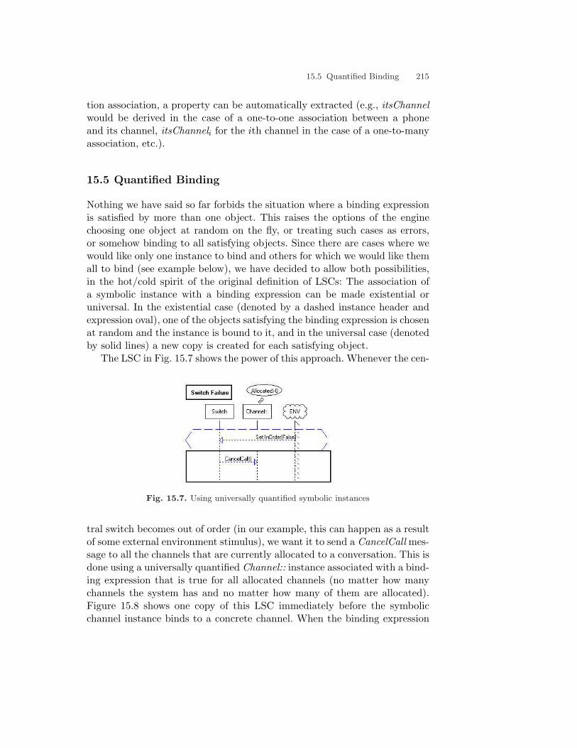
15.5 Quantified Binding 215
tion association, a property can be automatically extracted (e.g., itsChannelwould be derived in the case of a one-to-one association between a phoneand its channel, itsChanneli for the ith channel in the case of a one-to-manyassociation, etc.).
15.5 Quantified Binding
Nothing we have said so far forbids the situation where a binding expressionis satisfied by more than one object. This raises the options of the enginechoosing one object at random on the fly, or treating such cases as errors,or somehow binding to all satisfying objects. Since there are cases where wewould like only one instance to bind and others for which we would like themall to bind (see example below), we have decided to allow both possibilities,in the hot/cold spirit of the original definition of LSCs: The association ofa symbolic instance with a binding expression can be made existential oruniversal. In the existential case (denoted by a dashed instance header andexpression oval), one of the objects satisfying the binding expression is chosenat random and the instance is bound to it, and in the universal case (denotedby solid lines) a new copy is created for each satisfying object.
The LSC in Fig. 15.7 shows the power of this approach. Whenever the cen-
Fig. 15.7. Using universally quantified symbolic instances
tral switch becomes out of order (in our example, this can happen as a resultof some external environment stimulus), we want it to send a CancelCall mes-sage to all the channels that are currently allocated to a conversation. This isdone using a universally quantified Channel:: instance associated with a bind-ing expression that is true for all allocated channels (no matter how manychannels the system has and no matter how many of them are allocated).Figure 15.8 shows one copy of this LSC immediately before the symbolicchannel instance binds to a concrete channel. When the binding expression

216 15. Classes and Symbolic Instances
Fig. 15.8. Binding an instance during play-out
is evaluated, a different copy is created for each satisfying object. These LSCcopies are then added to the set of active copies and continue executing as ifthey were not created from the same original chart.
15.6 Reusing a Scenario Prefix
Figure 15.9(a) raises an interesting issue concerning multiple bindings of asymbolic instance. The LSC in the figure states that if some phone sends themessage Call(1) to the switch and then some other3 phone sends the samemessage to the switch, the switch sends an error message to the second phone.By way of illustration, suppose Phone1 is the first to send the message tothe switch. As a consequence, the left-hand instance in the chart is boundto Phone1. Now, Phone2 sends the message to the switch, the right-handinstance binds to Phone2, and the chart completes its execution by sendingthe error message from the switch to Phone2; see Fig. 15.9(b). This is fine.
Now suppose that a third phone, Phone3, sends the same message to theswitch. The pair of events of Phone1 and then Phone3 sending the samemessage satisfies the prechart of the LSC in Fig. 15.9(a), and the chart bodyshould therefore be executed. But this is a problem since after binding theright-hand instance to Phone2, the LSC copy completes execution and stopsexisting, and the first event of Phone1 sending the message is ‘lost’, making itimpossible for a second event to cause another satisfaction of the same chart.
We solve this problem as follows. When an instance in an already activatedLSC copy is bound to an object as the result of an event, the binding andconsequent propagation of the execution are carried out in a new separatecopy (in this case Fig. 15.9(b)). In addition, the original copy is left open,with the cut positioned as it was in the first active copy before the binding,3 The second calling phone must be different from the first one, recalling that an object
cannot be represented by more than one instance in an LSC.

15.6 Reusing a Scenario Prefix 217
Fig. 15.9. Retaining scenario prefixes for reuse
but with the symbolic instance in this remaining copy being restricted in abinding expression to not bind to the same object again. The original copyof Fig. 15.9(a), with its new binding expression, is shown in Fig. 15.9(c). Inthis way, prefixes of scenarios are kept open for reuse. Proceeding with ourexample, when Phone3 sends the message to the switch, a new copy is cre-ated, based on the original copy of Fig. 15.9(c), in which Phone3 is bound tothe right-hand instance. Then, in the original copy of Fig. 15.9(c), Phone3is added to the set of objects to which the right-hand instance cannot bind,thus making it possible for yet another phone to bind to this instance. Bythe way, during this described scenario, additional LSC copies are created.For example, each sending of Call(1) by Phone2 and Phone3 is also a mini-mal event and therefore causes the creation of new copies of this LSC; also,sending Call(1) by Phone3 after Phone2 completes the copy created whenPhone2 sent the message, etc. For clarity, we have focused here only on someof the copies.
If the engine determines that the set of forbidden objects of a symbolicinstance (together with the objects of the same class that are already presentin the chart and therefore cannot bind to the symbolic instance) becomes

218 15. Classes and Symbolic Instances
equal to the set of all objects in the system that are instances of the sameclass, the LSC copy is closed, since it has a symbolic instance that cannotbind to any more objects.
The same mechanism is adopted also for events that cause violation of aprechart. If an event e associated with object O occurs, and is unifiable withan event e′ associated with a symbolic instance I (among other things, thismeans, of course, that O is an instance of the class represented by I), and e′
is not enabled, this should be a violation. However, for the reasons discussedearlier, we want the scenario prefix to be kept open for other objects to bindto later. Therefore, a new copy is created, in which I is bound to O, and thiscopy is violated and closed.4 The original copy adds O to the set of restrictedobjects of I, thus forbidding O to bind to I later on in the execution.
15.7 Symbolic Instances in Existential Charts
In Chap. 12 we saw how existential charts can be used to specify systemtests and how they are monitored for successful completion. When an LSCis monitored, its events are propagated when matching events are generatedby the tested system. Since the events that are generated by the systemare actual events, in which the sending and receiving objects are concreteand known, there is no need for binding expressions in existential LSCs, andthe symbolic instances bind with concrete objects only as a result of systemevents.
Now, a universal LSC can also be monitored, but since when it is createdwe do not specify whether it is going to be used for execution or monitoringor both, binding expressions are used anyway. Therefore, even in the caseof monitoring a universal chart, instances can bind to concrete objects inbetween system events, as a result of evaluating binding expressions.
15.8 An Advanced Example: NetPhone
Using the NetPhone GUI and the play-in methodology, one can specify avariety of behaviors for the telephone network. In this section we show asimple, but non-trivial example of describing a requirement for this system,which strongly utilizes symbolic instances. The requirement, which involvesa phone setting its own number, is as follows:
When the user dials a number and then clicks the Set button, then:4 Creating a copy, violating it and closing it is done so that the user can be visually notified
of the effects of this most recent event.
15.8 An Advanced Example: NetPhone 219
1. If the number is already occupied by another phone an error mes-sage is shown.
2. Otherwise, the number is associated with the current phone asits telephone number, and is stored in the database as such. Thenumber is also displayed in the top-left corner of the phone’s GUI.
Since our GUI does not contain a database object, we first add it as aninternal object, called PhoneDB, and we can then play in the requirement. Wenow discuss this behavior in some detail, since it entails a chain of messagesgoing from the phone to the switch, from there to the database, and thenback to the phone. Note that in our model each phone is associated with aunique ID. This ID serves only to distinguish between the phone objects, andis different from the phone’s number, which is used to call the phone fromother phones. The channels are also associated with unique IDs that serve todistinguish between them, and it will be convenient to associate each phonewith the channel that has the same ID. Other 1–1 relations between phonesand channels could have been established in various different ways.
The LSC ‘Click Set’ (Fig. 15.10(a)) shows that when the user clicks the Setbutton the phone’s ID number, Phone.ID, is stored in the variable ID and thecurrently displayed number is stored in N. The phone then calls the switch’sSetNumber method with ID and N. The LSC ‘Verify Number’ (Fig. 15.10(b))shows that when some phone (the instance is symbolic but dashed) callsthe switch’s SetNumber method with parameters ID and N, the PhoneDBis searched for a phone ID associated with the number N (denoted by theimplemented function RetrieveKey). If the result returned in the PhoneDBstate variable QResult is the empty string(denoted by no value in the condi-tion), then no phone is associated with this number, and the switch thereforeasks the PhoneDB to associate the phone’s ID with the number N and tostore this information in the database. Otherwise, if the retrieved ID is notthe same as the initiating phone ID, the number N is already associated witha different phone, and an error message should be shown on the initiatingphone’s display. LSC ‘Set in DB’ (Fig. 15.10(c)) shows that when the switchasks the PhoneDB to associate the phone that has an ID equal to the num-ber stored in the variable ID with the number stored in the variable N , thePhoneDB actually stores the information in the DB (using an implementedfunction). If the operation was successful, the switch sends AckNumber tothe phone, which has an ID equal to ID. Otherwise, an error message is sentto this phone, indicating that the operation of linking the ID with the newnumber has failed. The final LSC, ‘AckNumber’ (Fig. 15.10(d)), simply statesthat when a phone receives the AckNumber message with the acknowledgednumber N as a parameter, the phone’s number is set to N (which, in turn,

220 15. Classes and Symbolic Instances
Fig. 15.10. A phone setting its own number
is reflected in the GUI by showing this number on the top-left corner of thephone) and the phone’s display is cleared by showing an empty string.
We have extended the NetPhone to include LSCs for establishing calls,answering calls, conference calls, hanging up, and many other scenarios. Ourmethod of using binding expressions to characterize symbolic instances al-lows each phone to set its phone number at runtime, but to use the numberproperty in binding expressions in order to refer to the required phone whendescribing interactions between telephones. This could not have been doneusing static instances and relationships only.
15.9 And a Bit More Formally ...
Here are the extensions and modifications needed to support symbolic in-stances and their binding during execution.

15.9 And a Bit More Formally ... 221
System Model and Events
The system model we have defined so far already contains classes and definesthe relationships between classes and objects. Hence, no modifications areneeded here.
LSC Specification
Until now, all we needed to know about an LSC instance was the object itrepresented, and this was given by the AppObj function. Since instances cannow be symbolic, and thus represent classes rather than objects, we modifythe definition of an instance as follows:
I = 〈`,O, C, ψ,Mode, Φ〉
where O ∈ O ∪ {⊥} is the concrete object represented by I (with O = ⊥if I is symbolic), C ∈ C ∪ {⊥} is the class represented by I (with C = ⊥if I is not symbolic), ψ ∈ {P × Oper × RHS} is the binding expression ofI, which is a basic condition expression restricting the property P ∈ C.P tocertain values, as discussed in Chap. 9, Mode ∈ {Existential, Universal} isthe instance quantification, and Φ ⊆ O is a set of forbidden objects that theinstance is not allowed to bind to. We also modify the range of AppObj toreflect these changes:
AppObj :⋃
L∈SIL → O ∪ C
We will use the predicate symbolic(I) as an abbreviation of I.C 6= ⊥. We nowdefine the relation X 4 Y , where X ∈ O and Y ∈ O ∪ C, to denote thateither X and Y are the same object or Y is the class to which X belongs:5
X 4 Y , (X ∈ O ∧ (X = Y ∨ class(X) = Y ))
We extend the relation 4 so it can also have instances as arguments in thenatural way (i.e., the relation refers to the objects or classes represented bythe instances).
The instances to which an LSC message M ∈ ML refers can now besymbolic. Therefore, we relax the requirement that the instances representthe same concrete objects as in the associated system message, and allowthem to also represent the classes to which the concrete objects belong:
M = 〈ISrc, IDst,MS〉5 Recall from Chap. 4 that every object belongs to exactly one class.

222 15. Classes and Symbolic Instances
where MS .Src 4 AppObj(ISrc) and MS .Dst 4 AppObj(IDst).We now extend EL, the set of LSC events, with the hidden event of binding
a symbolic instance with a concrete object:
EL =({m ∈ ML | m.Ms ∈ ΣFromUser ∪ΣToUser ∪ΣFromEnv ∪ΣToEnv ∪ΣCalls}× {Send, Recv})
∪ ({m ∈ ML | m.Ms ∈ ΣSelf} × {Send})∪ (PchL × {Start, End}) ∪ {Completed}∪ {perform(A) | A ∈ AL} ∪ {eval(C) | C ∈ CL}∪ (SUBL × {Start, End}) ∪ {branch(ITE)| ITE ∈ ITEL}∪ (LOOPL × {Start, End})∪ {skip(Loop)| Loop ∈ LOOPL ∧ Loop.Kind = Dynamic}∪ {bind(I)| I ∈ IL ∧ symbolic(I)}
The events of binding symbolic instances with concrete objects do not referto bindings that occur as a result of unifying events, but only to the actof binding a symbolic instance when its binding expression is enabled. Asopposed to all the other events we have seen so far, a bind(I) event is enabledwhen all the variables it uses are bound, regardless of the instances’ locationsas depicted by the current cut.
Operational Semantics
Prior to the addition of symbolic instances, one could tell whether two LSCmessages were unifiable by looking only at their associated system messages.Hence, the definition for message unification was:
Definition 15.9.1 (message unification). Two system messagesMs = 〈Src, Dst, P, V, f, λF
f , m, λMm , Symbolic〉 and
M ′s = 〈Src′, Dst′, P ′, V ′, f ′, λF
f ′ ,m′, λM
m′ , Symbolic′〉 are Q-unifiable (whereQ is ‘positively’ or ‘negatively’) if Src = Src′, Dst = Dst′, P = P ′,m = m′
and their contents are Q-unifiable.
This definition then served in the definition of unifiable events as follows:
Definition 15.9.2 (level1-unification).
1. A system event es = 〈ms, t〉 and an LSC event el = 〈ml, t′〉, with
t, t′ ∈ {Send, Recv} are Q-level1-unifiable (where Q is ‘positively’ or ‘neg-atively’) if t = t′, ml.Ms and ms are Q-unifiable, AppObj(ml.ISrc) =ms.Src, and AppObj(ml.IDst) = ms.Dst.

15.9 And a Bit More Formally ... 223
2. Two LSC events e = 〈m, t〉 and e′ = 〈m′, t′〉, with t, t′ ∈ {Send, Recv},are Q-level1-unifiable if t = t′, m.Ms and m′.Ms are Q-unifiable,AppObj(m.ISrc) = AppObj(m′.ISrc) and AppObj(m.IDst) =AppObj(m′.IDst).
Since we are never really interested in unifying two system events butrather in unifying a system event with an LSC event or unifying two LSCevents, and since the unification now depends also on the LSC instances, wemust modify these two definitions. First, we do not check the actual objectsof the system messages but rather leave this check to the event unification.Second, we no longer require the objects to be identical, and it suffices thatone is an instance of the other.
Definition 15.9.3 (message unification). Two system messagesMs = 〈Src, Dst, P, V, f, λF
f , m, λMm , Symbolic〉 and
M ′s = 〈Src′, Dst′, P ′, V ′, f ′, λF
f ′ ,m′, λM
m′ , Symbolic′〉 are Q-unifiable (whereQ is ‘positively’ or ‘negatively’) if they represent the same property or method(i.e., P = P ′ and m = m′), and their contents are Q-unifiable.
Definition 15.9.4 (level2-unification).
1. A system event es = 〈ms, t〉 and an LSC event el = 〈ml, t′〉, with
t, t′ ∈ {Send, Recv}, are Q-level2-unifiable (where Q is ‘positively’ or‘negatively’) if t = t′, ml.Ms and ms are Q-unifiable, ms.Src 4 ml.ISrc,ms.Src /∈ ml.ISrc.Φ, ms.Dst 4 ml.IDst, and ms.Dst /∈ ml.IDst.Φ.
2. Two LSC events e = 〈m, t〉 and e′ = 〈m′, t′〉, with t, t′ ∈ {Send, Recv},are Q-level2-unifiable if t = t′, m.Ms and m′.Ms are Q-unifiable and
((m.ISrc 4 m′.ISrc ∧ AppObj(m.ISrc) /∈ m′.ISrc.Φ)∨ (m′.ISrc 4 m.ISrc ∧ AppObj(m′.ISrc) /∈ m.ISrc.Φ))
and((m.IDst 4 m′.IDst ∧ AppObj(m.IDst) /∈ m′.IDst.Φ)∨ (m′.IDst 4 m.IDst ∧ AppObj(m′.IDst) /∈ m.IDst.Φ))
So far, the effect of unifying events was a possible binding of variables withnew values. However, now, unifying events may result also in binding symbolicinstances with concrete objects. We therefore define the act of unifying twolevel2-unifiable LSC events e = 〈m, t〉 and e′ = 〈m′, t〉 as follows:

224 15. Classes and Symbolic Instances
Unify(e, e′, Context)
1. Unify(e.m, e′.m′, Context).2. If symbolic(e.m.ISrc) and e′.m′.ISrc 4 e.m.ISrc then bind the sym-
bolic instance with the concrete object:a) e.m.ISrc.O ← e′.m′.ISrc.O.b) e.m.ISrc.C ← ⊥.
3. If symbolic(e′.m′.ISrc) and e.m.ISrc 4 e′.m′.ISrc then bind thesymbolic instance with the concrete object:a) e′.m′.ISrc.O ← e.m.ISrc.O.b) e′.m′.ISrc.C ← ⊥.
4. If symbolic(e.m.IDst) and e′.m′.IDst 4 e.m.IDst then bind the sym-bolic instance with the concrete object:a) e.m.IDst.O ← e′.m′.IDst.O.b) e.m.IDst.C ← ⊥.
5. If symbolic(e′.m′.IDst) and e.m.IDst 4 e′.m′.IDst then bind thesymbolic instance with the concrete object:a) e′.m′.IDst.O ← e.m.IDst.O.b) e′.m′.IDst.C ← ⊥.
A system event es = 〈ms, t〉 and an LSC event el = 〈ml, t〉 are also unifiedalong the same lines, except that the system event is guaranteed to haveconcrete objects as the sender and receiver of the message:
Unify(es, el, Context)
1. Unify(es.ms, el.ml, Context).2. If symbolic(el.ml.ISrc) and es.ms.Src 4 el.ml.ISrc then bind the
symbolic instance with the concrete object:a) el.ml.ISrc.O ← es.ms.Src.b) el.ml.ISrc.C ← ⊥.
3. If symbolic(el.ml.IDst) and es.ms.Dst 4 el.ml.IDst then bind thesymbolic instance with the concrete object:a) el.ml.IDst.O ← es.ms.Dst.b) el.ml.IDst.C ← ⊥.
The transition relation ∆[SO,SC ] should now be modified to contain alsothe effects of binding symbolic instances caused by event unification, andextended with transitions for handling the hidden events of binding symbolicinstances as their binding expressions become enabled:
• If e = 〈M, t〉 (where t ∈ {Send, Recv}) then:1. Set Context ← ∅.

15.9 And a Bit More Formally ... 225
2. If ∃CL ∈ SC and ∃e′ ∈ CL.LSC, such that e and e′ are negativelylevel2-unifiable and e′ violates CL, then:
a) Set SC ← SC \ {CL}.b) If temp(CL.Cut) = hot, set Violating ← True.c) If symbolic(e′.M.ISrc) or symbolic(e′.M.IDst) then create an identical
copy C ′L of CL, set SC ← SC ∪ {C ′L}, and in the copy sete′.M.ISrc.Φ ← e′.M.ISrc.Φ ∪ {e.M.Src} if symbolic(e′.M.ISrc)e′.M.IDst.Φ ← e′.M.IDst.Φ ∪ {e.M.Dst} if symbolic(e′.M.IDst)
3. For every universal LSC L ∈ SO which has an event e′, positively level2-unifiable with e, as a minimal event in its prechart, create a copy ofL, CL, and set SC ← SC ∪ {CL}. Set CL.Mode = PreActive and setits cut by CL.Cut ← AdvanceCut(InitialCut(L), 〈PchL, Start〉). Unifythe variables of e and e′, by Unify(e, e′, Context). For each hidden evente′′ <L e′, apply ∆(e′′).
4. For every existential LSC L ∈ SO which has an event e′, positively level2-unifiable with e, as a minimal event in the chart body, create a copy ofL, CL, and set SC ← SC ∪{CL}. Set CL.Mode = Check, and set its cutto the beginning of the chart by CL.Cut ← BeginMainCut(CL.LSC).Unify the variables of e and e′, by Unify(e, e′, Context). For each hiddenevent e′′ <L e′, apply ∆(e′′).
5. For every copy CL ∈ SC that has a reachable event e′ positively level2-unifiable with e:
a) If symbolic(e′.M.ISrc) or symbolic(e′.M.IDst) then create an identicalcopy of CL, C ′L, set SC ← SC ∪ {C ′L}, and in the copy set
e′.M.ISrc.Φ ← e′.M.ISrc.Φ ∪ {e.m.Src} if symbolic(e′.M.ISrc)e′.M.IDst.Φ ← e′.M.IDst.Φ ∪ {e.m.Dst} if symbolic(e′.M.IDst)
b) Set CL.Cut ← AdvanceCut(CL.Cut, e′).c) If e′ = 〈M,Send〉, M is synchronous and e′′ = 〈M, Recv〉,
set CL.Cut ← AdvanceCut(CL.Cut, e′′).d) Unify the events e and e′, Unify(e, e′, Context).e) For each hidden event e′′ <L e′, apply ∆(e′′).
• If e = Completed(CL) for some CL ∈ SC , then set SC ← SC \ {CL}.• If e = 〈PchL, End〉 for some CL ∈ SC , then set
CL.Cut ← BeginMainCut(CL.LSC) and CL.Mode ← Active.• If e = perform(A) for some A ∈ AL s.t. CL ∈ SC , then set CL.Cut ←
AdvanceCut(CL.Cut, e) and set
A.V ←
A.C if A.Type = constantV alue(A.P ) if A.Type = propertyA.f(A.λF
f ) if A.Type = function

226 15. Classes and Symbolic Instances
• If e = eval(C) for some C ∈ CL s.t. CL ∈ SC then1. If value(C) = true then set CL.Cut ← AdvanceCut(CL.Cut, e).2. If value(C) = false then
a) If subchart(C) ∈ {ITE.SubT , ITE.SubE} for some ITE then
set CL.Cut ← AdvanceCut(CL.Cut, (ITE,End))
b) If subchart(C) = Sub ∈ SUBL then
set CL.Cut ← AdvanceCut(CL.Cut, (Sub, End))
c) If subchart(C) = ⊥ then set SC ← SC \ {CL}.d) If temp(C) = hot then set Violating ← True.
• If e = branch(ITE) for some ITE ∈ CL s.t. CL ∈ SC then1. If value(ITE.C) = true then set
CL.Cut ← AdvanceCut(CL.Cut, (ITE.SubT , Start)).2. If value(ITE.C) = false then
set CL.Cut ←{
AdvanceCut(CL.Cut, (ITE.SubE , Start)) if ITE.SubE 6= ⊥AdvanceCut(CL.Cut, (ITE.SubT , End)) if ITE.SubE = ⊥
• If e = (ITE.SubT , End) for some ITE ∈ CL s.t. CL ∈ SC then
set CL.Cut ← AdvanceCut(CL.Cut, (ITE,End))
• If e = (ITE.SubE , End) for some ITE ∈ CL s.t. CL ∈ SC then
set CL.Cut ← AdvanceCut(CL.Cut, (ITE.SubE , End))
• If e = (Sub, End) for some Sub ∈ CL s.t. CL ∈ SC then
set CL.Cut ← AdvanceCut(CL.Cut, (Sub, End))
• If e = skip(Loop) for some Loop ∈ CL s.t. CL ∈ SC then
set CL.Cut ← AdvanceCut(CL.Cut, (Loop,End))
• If e = (Loop, Start) for some Loop ∈ CL s.t. CL ∈ SC then
set CL.Cut ← AdvanceCut(CL.Cut, (Loop, Start))
For every variable V ∈ VL that is used in Loop for the first time, setV.ω ← ⊥.
• If e = (Loop, End) for some Loop ∈ CL s.t. CL ∈ SC and Loop.Kind 6=Dynamic then

15.10 Bibliographic Notes 227
1. Set µ ← µ− 1.2. If µ > 0 then
set CL.Cut ← AdvanceCut(CL.Cut, (Loop, Start))
For every variable V ∈ VL that is used in Loop for the first time, setV.ω ← ⊥.
3. If µ = 0 then
set CL.Cut ← AdvanceCut(CL.Cut, (Loop,End))
• If e = bind(I) for some symbolic instance I ∈ CL s.t. CL ∈ SC , then:1. S ← {O ∈ O | O 4 I, O satisfies I.ψ and @I ′ ∈ CL s.t. I ′.O = O}.2. If S = ∅ then SC ← SC \ {CL}.3. If I.Mode = Existential then
a) Set I.O = O, for some O ∈ S.b) Set I.C = ⊥.
4. If I.Mode = Universal then perform the following for every O ∈ S:a) Create an identical copy C ′L of CL.b) Set SC ← SC ∪ {C ′L}.c) Set I.O = O.d) Set I.C = ⊥.Finally, set SC ← SC \ {CL}.
Since the events of binding symbolic instances with objects that satisfytheir binding expressions are simply additional forms of hidden events, theprocedures step, super-step and monitor-event handle them with no modifi-cations needed.
15.10 Bibliographic Notes
Deriving object relations from the object model diagram and utilizing theserelations during execution was discussed in [44] and is implemented in theRhapsody tool [60].
Extending LSCs with symbolic instances was first described in [84]. In thatpaper we also discuss the rather technical problem of redundant activation ofsymmetric precharts, and a proposed solution. However, since the issue is nottreated in the current implementation of the Play-Engine, we have decidedto omit it from the book.
In [64] there is a description of work (carried out independently of ours)that deals with relating instance lines in LSCs to objects and classes, as part

228 15. Classes and Symbolic Instances
of an ongoing effort to establish a verification environment for UML models.The resulting decisions made in [64] are different from ours, since the goalswere quite different; we have executability of LSCs as one of our main goals,while the main purpose of LSCs in [64] is to serve as a basis for testing anintra-object model or implementation.

16. Time and Real-Time Systems
In this chapter, we extend the language of LSCs and the Play-Engine withmeans for dealing with time. We use a single discrete clock that is linkedto the host computer’s internal clock. We also assume the synchrony hy-pothesis. Hence, in terms of playing out the behavior on an actual simulatingcomputer, we essentially have a real-time mechanism. The resulting extensionis extremely expressive.
16.1 An Example
Let us return to the cellular phone example, and consider the requirementdiscussed in Chap. 7:
Every time the user opens or closes the cover, the antenna shouldautomatically open or close as well.
The LSC in Fig. 16.1 captures this requirement. Now, suppose we change therequirement as follows:
Every time the user opens or closes the cover, the antenna shouldautomatically open or close between two and four seconds later.
This requirement refers to the time passage between events, and in order toexpress it we have to extend the language of LSCs with timing constructs.The LSC in Fig. 16.2 shows how this requirement is expressed in the extendedlanguage. After the cover is opened (closed), the current time is stored in thevariable T . Before the antenna is allowed to open (close) we make sure, usinga hot condition, that the current time is greater than or equal to T +2. Sincea hot condition must be met, the execution must wait until the conditionbecomes true, thus forcing the required delay. Finally, after the antenna opens(closes), we check, again using a hot condition, that the current time is nomore than T + 4, thus making sure that the interval’s upper bound was notviolated.

230 16. Time and Real-Time Systems
Fig. 16.1. Opening and closing the antenna automatically
Fig. 16.2. Opening and closing the antenna within a specified time interval
16.2 Adding Time to LSCs
Many kinds of reactive systems must explicitly refer to time and react to itspassage. For this purpose, a variety of programming language constructs havebeen proposed, including delays, timeouts, watchdogs and clock variables.Temporal logic, for example, has been extended by a variety of constructs toenable quantification of time, including bounded temporal operators, freezequantifiers and the use of explicit clock variables. Visual scenario-based lan-guages, such as MSCs, have also been extended with timers, delay intervals,

16.3 Hot Timing Constraints 231
drawing rules and timing marks. Many of these approaches are referred to inthe bibliographic notes at the end of this chapter.
To extend the language of LSCs to deal with time, we adopt the basicphilosophy of Alur and Henzinger, according to which a real-time system canbe viewed as a discrete system with clock variables. We apply this approach inour setting by adding a special single clock object with one property, Time,and one method, Tick. The new object and its method can be referred to inthe charts by a special instance (with a clock icon) and a special constantTick event. The main technical observation underlying this chapter is that byusing these new elements with constructs already existing in our language,such as assignments and conditions, and, significantly, by exploiting the hotand cold dichotomy that pervades our entire approach, we are able to capturea rich set of timing constraints and time-based behavior.
An important point here is that we have chosen to assume the synchronyhypothesis, although we did not have to do so in order to make semanticsense of our extension. This is a well-known abstraction of real-time systems,according to which the system events themselves consume no actual time,and time may pass only between events. As we shall see later, the synchronyhypothesis makes our life a bit simpler when it comes to executing a time-enriched LSC specification.
16.3 Hot Timing Constraints
A timing constraint in the extended LSC language can be defined by a combi-nation of assignments and conditions. Figure 16.3 shows how to express threeof the most common timing constraints in scenario-based visual languages.A vertical delay interval indicates the minimal and maximal delays allowedbetween two consecutive events along an instance line. Such an interval is ex-pressed in our language using the following steps (see Fig. 16.3(a), and notethe small sand-clock icons added to the assignment and condition boxes):
Store time: The time is stored immediately after the first event. Accordingto our semantics, assignments are performed as soon as they are reached.Hence, the value of the variable will be the time instant at which theevent occurs.
Specify minimal delay: The minimal delay is specified by placing a hot con-dition of the form Time > Time-Variable + Min-Delay just before thesecond event. According to the described semantics, hot conditions areevaluated continuously until they become true. Therefore, this conditionwill be advanced only after the required period has passed. Such a condi-

232 16. Time and Real-Time Systems
Fig. 16.3. Expressing common timing constraints in LSCs
tion may be reached after the required lower bound on time has passed,in which case it will be advanced immediately.
Specify maximal delay: The maximal delay is specified by placing a hot con-dition of the form Time < Time-Variable + Max-Delay just after thesecond event. If the condition is reached before the maximal delay haselapsed, it will evaluate to true and will be advanced immediately, caus-ing no delay or violation. If the condition is reached after the maximaldelay has elapsed, it evaluates to false, and since time cannot decrease thecondition will never hold and it is therefore treated as a constant Falsecondition, causing a violation of the requirements.
A message delay interval indicates the minimal and maximal delaysallowed from the moment a message is sent until it is received. This kind ofdelay interval is specified like a vertical delay, except that here the time isstored on one instance line and is checked on another (Fig. 16.3(b)). Note thatthe assignment and the first condition in the figure are not related by the LSCpartial order, so that the condition may be reached before the assignment.However, recall that a condition that uses (refers to) an unbound variablecannot be evaluated. Thus, in this case, the condition will not be evaluateduntil the assignment is performed.
The ITU-TS Recommendation Z.120 document provides timers for ex-pressing timing constraints within a single MSC, and along a single instance.Such a timer can be set to a value, reset to 0, and observed for timeout, andcan be used to express a minimal delay between two consecutive events ora maximal delay between two or more consecutive events. However, timerscannot be shared among different instances in an MSC and can thereforebe used to constrain events occurring only within a single object. Our LSC
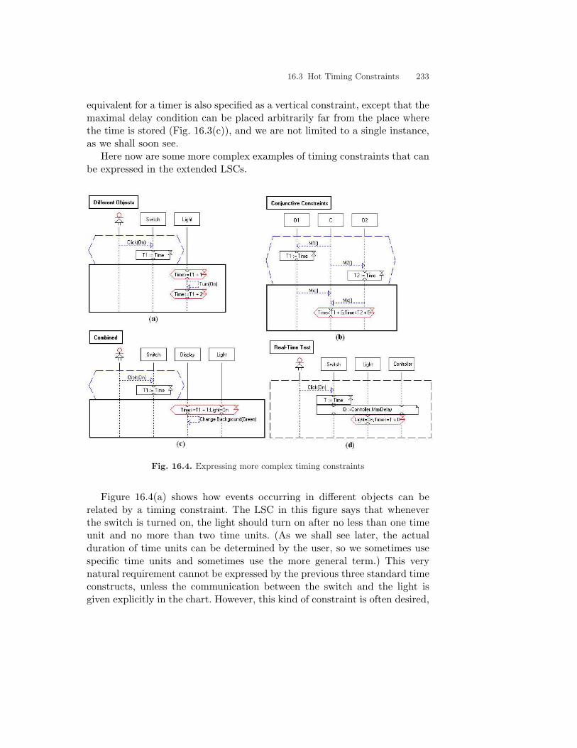
16.3 Hot Timing Constraints 233
equivalent for a timer is also specified as a vertical constraint, except that themaximal delay condition can be placed arbitrarily far from the place wherethe time is stored (Fig. 16.3(c)), and we are not limited to a single instance,as we shall soon see.
Here now are some more complex examples of timing constraints that canbe expressed in the extended LSCs.
Fig. 16.4. Expressing more complex timing constraints
Figure 16.4(a) shows how events occurring in different objects can berelated by a timing constraint. The LSC in this figure says that wheneverthe switch is turned on, the light should turn on after no less than one timeunit and no more than two time units. (As we shall see later, the actualduration of time units can be determined by the user, so we sometimes usespecific time units and sometimes use the more general term.) This verynatural requirement cannot be expressed by the previous three standard timeconstructs, unless the communication between the switch and the light isgiven explicitly in the chart. However, this kind of constraint is often desired,

234 16. Time and Real-Time Systems
especially in the requirements analysis phase, without having to get into thedetails of implementation.
Figure 16.4(b) shows the use of conjunctive timing constraints. The LSCshows a scenario where object C sends messages to O1 and O2 and expectsmessages in reply from both objects. C is willing to accept the replies no laterthan five time units after the first object received its message. Conjunctivetiming constraints are very useful when it is impossible to know the exactexecution order between multiple events that can affect some other event.
Figure 16.4(c) shows how conditions can be used to combine timing con-straints with conventional constraints. In this LSC, when the switch is turnedon, the display should change its background color to green, but only if thelight is on, and no earlier than 1 time unit after the switch event. When thecondition is reached, execution will be advanced only if and when both ofthese are true.
The combination of real-time constraints and regular ones can be takenone step further, as seen in Fig. 16.4(d). This is an existential LSC, whichdescribes a simple test stating our expectation that the light should be on nomore than D time units after the switch was turned on. Or, in other words,that if the light is still off later than D units after the switch was turned on,we are in trouble. The value of D is taken from the MaxDelay state variable ofthe controller, which may change dynamically during the system run. Notethat since this LSC represents a test, it does not have to specify how theresult of the light being on is achieved but only that it indeed is.
16.4 Cold Timing Constraints
In the previous section we used hot conditions to force an event to occuronly after a certain amount of time has elapsed (by a minimal delay) andto cause a violation if the constraint is not satisfied (by a maximum delay).The availability of cold conditions further enriches the expressive power oftime-enriched LSCs. A cold timing constraint with a minimal delay statesthat if a certain event occurs after a specified period of time, the scenariocontinues, otherwise the chart is exited. A cold constraint with a maximaldelay states that if the event occurred within the specified period of time,the chart (or subchart) continues, otherwise the rest of it is simply ignored.
Figure 16.5 shows an example. The Queen of Hearts instructs the rabbit tocome to her palace in five seconds, and proceeds to look at her watch, notingthe time. The rabbit meets Alice and tells her he is late (the message is cold,so he doesn’t have to do this, but can). Alice hurries the rabbit up, and uponarriving at the Queen’s palace he reports to her. The Queen then checks

16.5 Time Events 235
Fig. 16.5. Having a cold time in Wonderland
whether more than five seconds have passed since the last time she looked ather watch. If this is the case, she issues an order to remove the rabbit’s head;otherwise, the scenario ends with the rabbit’s anatomy intact. . .
16.5 Time Events
Reactive real-time systems are often required to react to the passage of time,and not only to refer to it when constraining the timing of other events ofinterest. An example of such a requirement could be:
The controller should probe the thermometer for a temperature valueevery 100 milliseconds, and if the result is more than 60 degrees, itshould deactivate the heater and send a warning to the console.
To express such requirements, generally termed time events, a special objectinstance representing the clock is available, and can it be added to the LSCs.Within this instance one can refer to the Tick event, which represents anactual clock tick, i.e., the passage of a single time unit. This event can beplaced in a prechart to trigger desired actions, or in the main chart, thusexplicitly forcing delays.
Figure 16.6 shows an LSC that describes the above requirement.

236 16. Time and Real-Time Systems
Fig. 16.6. Time events in LSCs
16.6 Playing In
In order for the user to be able to refer to time while remaining within theintuitive convenience of GUI-oriented play-in, we have added a global clockobject (accessible directly from the upper toolbar of the engine’s layout: seeFig. 16.7). To specify a Tick event, the user simply clicks the clock’s Tickbutton on the toolbar.
Fig. 16.7. The clock object in the Play-Engine’s toolbar
In order to specify timing constraints, the user needs to store time in timevariables and to restrict time with respect to these variables. Although weuse the existing constructs of assignments and conditions for these activities,the Play-Engine provides more direct ways to define the timed versions ofthese constructs.
To store the time at any point during play-in, the user right-clicks the rele-vant object and chooses Store Time from the popup menu (see Fig. 16.8(a)).In response, the Play-Engine displays a popup dialog in which the user is re-quested to name the time variable.
To specify a timing constraint, the user right-clicks the constrained objectand chooses Time Constraint. . . from the popup menu (Fig. 16.8(b)). Inresponse, a timing constraint dialog opens up, in which the user specifies thetime variable, the delay and the constraint operator (Fig. 16.8(c)).

16.7 Playing Out 237
Fig. 16.8. Playing in a timing constraint
We have also added the following feature to the Play-Engine’s interface:placing the mouse over a timed assignment causes the engine to draw thinindication lines from it to all the timing constraints it may affect (see Fig.16.2), and placing it over a timing constraint shows such lines drawn to allthe timed assignments that may affect it. We should add that the algorithmfor doing this is non-trivial, as it has to take into account the partial orderin the chart, the bindings of variables, and a number of additional things.1
16.7 Playing Out
As emphasized throughout the book, our target is not merely to constructan off-line modeling medium, but to produce an executable formalism —for which the execution mechanism essentially constitutes the operationalsemantics — and to build the tool that executes the specifications. Thesegoals raise a host of new issues when time is included as part of the language,and this section discusses the way we deal with them.
We have already seen that during execution the Play-Engine generatesonly system events; it does not cause events that should be triggered by theuser or by the external environment. In this sense, the clock is considered part1 We have actually implemented this algorithm for assignments and conditions in general,
and not only for those that deal with time.

238 16. Time and Real-Time Systems
of the system’s external environment, and the Play-Engine does not triggerclock ticks on its own. Hence, in contrast to time-less LSCs, here a super-stepcan terminate in the middle of a chart’s body because of as-yet unsatisfiedminimal-delay constraints.
So how indeed does our clock tick during play-out? We have implementedtwo means for this. The first is a manual mode, where the user can causea tick by simply clicking the Tick icon on the engine’s toolbar. Note thatgiving the user the power to control clock ticks, over and above the abilityto cause normal external events, makes it possible to trigger several eventswithin a single time unit, which can be used to set up realistic scenarios,since it is often the case that a real-world external environment is capable ofdoing exactly that.
The second mode is an automatic one. Here, the Play-Engine triggersa clock tick every fixed interval, using the host machine’s internal clock toobtain the actual time information. The interval length, relative to the realclock, is determined by the engine’s user, and a natural thing to do would beto set the interval to be the time unit used in the requirements themselves,or the smallest such unit (e.g., if the time units are seconds, then the timeinterval could be set to 1000 ms). Allowing for true control over the exe-cution/simulation speed, at least insofar as the host machine’s clock allows,this gets us as close as can be hoped to having a ‘really’ real-time systemmodel (that is, on a general-purpose computer, as opposed to working on aspecial-purpose real-time operating system).2
The Play-Engine performs a lot of additional work during execution thatis not related to actually executing the specified events and actions (e.g.,finding the next event to be taken, monitoring the activated LSCs and dis-playing their progress graphically, etc.). Therefore, we have to somehow con-front the problem of model vs. implementation, which is particularly acutein the real-time arena. The synchrony hypothesis makes this easier. Whenour Play-Engine executes the model, the clock keeps ticking and the systemwaits for external stimuli. When such a stimulus arrives, our execution mech-anism freezes the clock and performs the sequence of events that constitutesthe system’s response to that stimulus (this is the super-step). When the se-quence is completed, the clock’s operation is resumed, thus causing the effectof zero-time actions. We could just as easily not adopt the synchrony as-sumption that freezes the clock when this kind of additional engine-specific‘meta-work’ is carried out, but rather let the clock continue to tick whenevents and functions from the model itself are applied. However, doing sowould mean that since the Play-Engine executes on a single-processor PC2 If the interval between ticks is made sufficiently large, the user can trigger several end-
user and environment events within a single time unit in this mode too.

16.8 Unification of Clock Ticks 239
the requirements are captured correctly only if the target system also runson a single-processor platform.
16.8 Unification of Clock Ticks
The clock Tick event is denoted in LSCs as a self message, going from theclock instance to itself. Although this message appears to be like any otherone, its unification with the Tick event must be handled in a special way. Toillustrate the problematic nature of this special message, consider the LSCin Fig. 16.9.
Fig. 16.9. Unification of Tick messages with the Tick event
This LSC says that every time the user clicks the PWR button, the displaywaits for three time units and then changes its color to green and then towhite, twice. Between every two changes of color there is a delay of at leastone time unit. The clock Tick event is being used here to explicitly indicatethe passage of time, as an alternative to the timing constraints describedearlier.
There is however a problem with this chart. In order to advance beyondthe first timing constraint, three time units must elapse. The passage of eachtime unit is caused by a Tick event, but as the first such event occurs it willbe unified with the Tick messages in the chart and will cause the chart’s

240 16. Time and Real-Time Systems
violation (because of the semantics of events, which causes violation if anevent occurs out of sequence). This problem complicates the task of specifyingtimed specifications, especially in the case where a Tick message must appearin the prechart, since having such a message forbids the occurrence of otherticks until the chart completes (unless these ticks are specified explicitly inthe chart body).
To overcome this problem we handle the unification of Tick events dif-ferently: Recall that we use positive unification when looking for events thatcan be propagated simultaneously, whereas we use negative unification to findevents that violate currently active LSCs. In the case of clock ticks, we do notwant the occurrence of a Tick event to be considered a violation because ofTick messages that appear elsewhere in the LSC. Therefore, Tick events canbe positively unified (so that minimal events are found and Tick messagesare advanced when required), but they are not negatively unifiable. Thus, aTick event in a chart does not prevent other Tick events from happening.
Chapter 17 discusses an alternative way of specifying that a Tick event isnot allowed to happen as long as a specific LSC is active.
16.9 The Time-Enriched NetPhone Example
In Chap. 15 we introduced the telephone network example, and used it toillustrate the power of symbolic instances. We now extend this NetPhonesystem with a number of time-related features. For example, Fig. 16.10(b)shows the LSC for an auto-dial feature:
If a phone that is not in automatic mode tries to call some number,following which the “Receiver Busy...” message appears on the dis-play, then if the user clicks the call button within five seconds fromthe time the message appeared, the phone enters automatic mode.
The LSC in Fig. 16.10(c) shows the behavior of a phone in automaticmode. As soon as it enters this mode the phone stores the current time inTs. It then displays “Automatic Mode”, and enters an (unbounded) loop,which iterates for as long as the display shows “Automatic Mode”, but nolonger than 30 seconds from when the mode was entered. The loop’s controlis captured by the cold condition therein, whose semantics prescribes exitingthe current subchart — i.e., the loop — upon becoming false. The first thingthe phone does inside the loop is to store the current time in T1 and to trycalling the desired number. It then waits one second for the communicationprotocol to be over and checks the message on the display. If it says “ReceiverBusy ...”, the display is set to show “Automatic Mode” again. Then there

16.9 The Time-Enriched NetPhone Example 241
Fig. 16.10. Some time-related behavior of the NetPhone system
is a hot constraint that forces a five second wait before there is an attemptto reconnect. After the loop, there is a cold time constraint: If the loop wasexited after 30 seconds or more (i.e., it was exited not because a conversationwas established), the display shows that the automatic mode has expired.
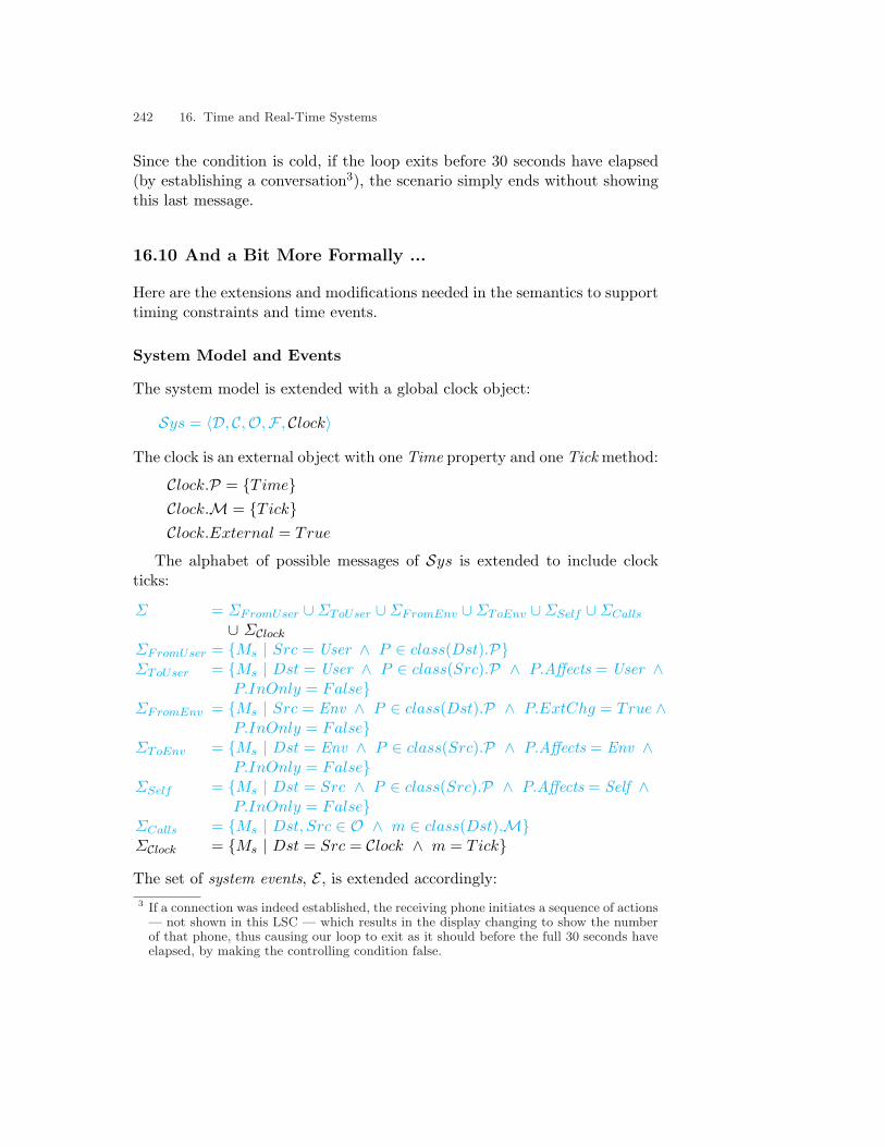
242 16. Time and Real-Time Systems
Since the condition is cold, if the loop exits before 30 seconds have elapsed(by establishing a conversation3), the scenario simply ends without showingthis last message.
16.10 And a Bit More Formally ...
Here are the extensions and modifications needed in the semantics to supporttiming constraints and time events.
System Model and Events
The system model is extended with a global clock object:
Sys = 〈D, C,O,F , Clock〉
The clock is an external object with one Time property and one Tick method:
Clock.P = {Time}Clock.M = {Tick}Clock.External = True
The alphabet of possible messages of Sys is extended to include clockticks:
Σ = ΣFromUser ∪ΣToUser ∪ΣFromEnv ∪ΣToEnv ∪ΣSelf ∪ΣCalls
∪ ΣClock
ΣFromUser = {Ms | Src = User ∧ P ∈ class(Dst).P}ΣToUser = {Ms | Dst = User ∧ P ∈ class(Src).P ∧ P.Affects = User ∧
P.InOnly = False}ΣFromEnv = {Ms | Src = Env ∧ P ∈ class(Dst).P ∧ P.ExtChg = True ∧
P.InOnly = False}ΣToEnv = {Ms | Dst = Env ∧ P ∈ class(Src).P ∧ P.Affects = Env ∧
P.InOnly = False}ΣSelf = {Ms | Dst = Src ∧ P ∈ class(Src).P ∧ P.Affects = Self ∧
P.InOnly = False}ΣCalls = {Ms | Dst, Src ∈ O ∧ m ∈ class(Dst).M}ΣClock = {Ms | Dst = Src = Clock ∧ m = Tick}The set of system events, E , is extended accordingly:3 If a connection was indeed established, the receiving phone initiates a sequence of actions
— not shown in this LSC — which results in the display changing to show the numberof that phone, thus causing our loop to exit as it should before the full 30 seconds haveelapsed, by making the controlling condition false.

16.10 And a Bit More Formally ... 243
E = ((ΣFromUser ∪ΣToUser ∪ΣFromEnv ∪ΣToEnv ∪ΣCalls)× {Send, Recv})∪ ((ΣSelf ∪ΣClock)× {Send})
LSC Specification
We modify the definitions of assignments and conditions so that they canrefer to time, as explained in the text.
An assignment is defined as:
A = 〈V, IA, C, P, f, λFf , T imed〉
where Timed ∈ {True, False} is a flag indicating whether A is a timedassignment. We require that one and only one of the following expressionsholds for each assignment:
(C 6= ⊥), (P 6= ⊥), (f 6= ⊥), (Timed = true)
We say that the assignment type of A is time if Timed = true.The set of a condition’s basic expressions is extended to include also timing
constraints:
ψ ∈ {LHS ×Oper ×RHS} ∪ {TRUE, FALSE, SELECT(P),⊥}∪ {Time×Oper × VL ×RHS}
whereLHS ∈ {O.P |O ∈ O, P ∈ O.P} ∪ VL
Oper ∈ {=, <,≤, >,≥, 6=}RHS ∈ (
⋃
D∈DD) ∪ VL ∪ {(f, λF
f )|f ∈ F}
A timing constraint is therefore a basic expression, in which the constrained(left) part is the reserved word Time, and the constraint is the sum of thevalues of a (time) variable and a delay. The latter can be any constant, vari-able or function expression. If ψ is a time constraint, value(ψ) is computedby evaluating ψ in the natural way, where Time is replaced by the currentvalue of Clock.T ime.
Finally, we extend EL, the set of LSC events, with the visible event of theclock ticking:

244 16. Time and Real-Time Systems
EL =({m ∈ ML | m.Ms ∈ ΣFromUser ∪ΣToUser ∪ΣFromEnv ∪ΣToEnv ∪ΣCalls}× {Send, Recv})
∪ ({m ∈ ML | m.Ms ∈ ΣSelf ∪ΣClock} × {Send})∪ (PchL × {Start, End}) ∪ {Completed}∪ {perform(A) | A ∈ AL} ∪ {eval(C) | C ∈ CL}∪ (SUBL × {Start, End}) ∪ {branch(ITE)| ITE ∈ ITEL}∪ (LOOPL × {Start, End})∪ {skip(Loop)| Loop ∈ LOOPL ∧ Loop.Kind = Dynamic}∪ {bind(I)| I ∈ IL ∧ symbolic(I)}
Operational Semantics
First, we modify the definition of message unification so that Tick events arenot negatively-unifiable.
Definition 16.10.1 (message unification). Two system messagesMs = 〈Src, Dst, P, V, f, λF
f , m, λMm , Symbolic〉 and
M ′s = 〈Src′, Dst′, P ′, V ′, f ′, λF
f ′ ,m′, λM
m′ , Symbolic′〉 are Q-unifiable (whereQ is ‘positively’ or ‘negatively’) if they represent the same property or methodP = P ′ ∧m = m′ and their contents are Q-unifiable. If m = m′ = Tick, Ms
and M ′s are only positively-unifiable.
The transition relation ∆[SO,SC ] is now modified to handle time assign-ments and time constraints correctly, and is also extended with transitionsfor handling the Tick event.
• If e = 〈M, t〉 (where t ∈ {Send, Recv}) then:1. If e.M.m = Tick then set Clock.T ime ← Clock.T ime + 1.2. Set Context ← ∅.3. If ∃CL ∈ SC and ∃e′ ∈ CL.LSC, such that e and e′ are negatively
level2-unifiable and e′ violates CL, then:a) Set SC ← SC \ {CL}.b) If temp(CL.Cut) = hot, set Violating ← True.c) If symbolic(e′.M.ISrc) or symbolic(e′.M.IDst) then create an identical
copy C ′L of CL, set SC ← SC ∪ {C ′L}, and in the copy sete′.M.ISrc.Φ ← e′.M.ISrc.Φ ∪ {e.M.Src} if symbolic(e′.M.ISrc)e′.M.IDst.Φ ← e′.M.IDst.Φ ∪ {e.M.Dst} if symbolic(e′.M.IDst)
4. For every universal LSC L ∈ SO which has an event e′, positively level2-unifiable with e, as a minimal event in its prechart, create a copy ofL, CL, and set SC ← SC ∪ {CL}. Set CL.Mode = PreActive and setits cut by CL.Cut ← AdvanceCut(InitialCut(L), 〈PchL, Start〉). Unifythe variables of e and e′, by Unify(e, e′, Context). For each hidden evente′′ <L e′, apply ∆(e′′).

16.10 And a Bit More Formally ... 245
5. For every existential LSC L ∈ SO which has an event e′, positively level2-unifiable with e, as a minimal event in the chart body, create a copy ofL, CL, and set SC ← SC ∪{CL}. Set CL.Mode = Check, and set its cutto the beginning of the chart by CL.Cut ← BeginMainCut(CL.LSC).Unify the variables of e and e′, by Unify(e, e′, Context). For each hiddenevent e′′ <L e′, apply ∆(e′′).
6. For every copy CL ∈ SC that has a reachable event e′ positively level2-unifiable with e:
a) If symbolic(e′.M.ISrc) or symbolic(e′.M.IDst) then create an identicalcopy of CL, C ′L, set SC ← SC ∪ {C ′L}, and in the copy set
e′.M.ISrc.Φ ← e′.M.ISrc.Φ ∪ {e.m.Src} if symbolic(e′.M.ISrc)e′.M.IDst.Φ ← e′.M.IDst.Φ ∪ {e.m.Dst} if symbolic(e′.M.IDst)
b) Set CL.Cut ← AdvanceCut(CL.Cut, e′).c) If e′ = 〈M,Send〉, M is synchronous and e′′ = 〈M, Recv〉,
set CL.Cut ← AdvanceCut(CL.Cut, e′′).d) Unify the events e and e′, Unify(e, e′, Context).e) For each hidden event e′′ <L e′, apply ∆(e′′).
• If e = Completed(CL) for some CL ∈ SC then set SC ← SC \ {CL}.• If e = 〈PchL, End〉 for some CL ∈ SC , then set
CL.Cut ← BeginMainCut(CL.LSC) and CL.Mode ← Active.• If e = perform(A) for some A ∈ AL s.t. CL ∈ SC , then CL.Cut ←
AdvanceCut(CL.Cut, e) and
A.V ←
A.C if A.Type = constantV alue(A.P ) if A.Type = propertyA.f(A.λF
f ) if A.Type = function
Clock.T ime if A.Type = time
• If e = eval(C) for some C ∈ CL s.t. CL ∈ SC then1. If value(C) = true then set CL.Cut ← AdvanceCut(CL.Cut, e).2. If value(C) = false then
a) If subchart(C) ∈ {ITE.SubT , ITE.SubE} for some ITE then
set CL.Cut ← AdvanceCut(CL.Cut, (ITE,End))
b) If subchart(C) = Sub ∈ SUBL then
set CL.Cut ← AdvanceCut(CL.Cut, (Sub, End))
c) If subchart(C) = ⊥ then set SC ← SC \ {CL}.d) If temp(C) = hot then set Violating ← True.
• If e = branch(ITE) for some ITE ∈ CL s.t. CL ∈ SC then

246 16. Time and Real-Time Systems
1. If value(ITE.C) = true then setCL.Cut ← AdvanceCut(CL.Cut, (ITE.SubT , Start))
2. If value(ITE.C) = false then
set CL.Cut ←{
AdvanceCut(CL.Cut, (ITE.SubE , Start)) if ITE.SubE 6= ⊥AdvanceCut(CL.Cut, (ITE.SubT , End)) if ITE.SubE = ⊥
• If e = (ITE.SubT , End) for some ITE ∈ CL s.t. CL ∈ SC then
set CL.Cut ← AdvanceCut(CL.Cut, (ITE,End))
• If e = (ITE.SubE , End) for some ITE ∈ CL s.t. CL ∈ SC then
set CL.Cut ← AdvanceCut(CL.Cut, (ITE.SubE , End))
• If e = (Sub, End) for some Sub ∈ CL s.t. CL ∈ SC then
set CL.Cut ← AdvanceCut(CL.Cut, (Sub, End))
• If e = skip(Loop) for some Loop ∈ CL s.t. CL ∈ SC then
set CL.Cut ← AdvanceCut(CL.Cut, (Loop,End))
• If e = (Loop, Start) for some Loop ∈ CL s.t. CL ∈ SC then
set CL.Cut ← AdvanceCut(CL.Cut, (Loop, Start))
For every variable V ∈ VL that is used in Loop for the first time, setV.ω ← ⊥.
• If e = (Loop, End) for some Loop ∈ CL s.t. CL ∈ SC and Loop.Kind 6=Dynamic then1. Set µ ← µ− 1.2. If µ > 0 then
set CL.Cut ← AdvanceCut(CL.Cut, (Loop, Start))
For every variable V ∈ VL that is used in Loop for the first time, setV.ω ← ⊥.
3. If µ = 0 then
set CL.Cut ← AdvanceCut(CL.Cut, (Loop,End))
• If e = bind(I) for some symbolic instance I ∈ CL s.t. CL ∈ SC , then:1. S ← {O ∈ O | O 4 I, O satisfies I.ψ and @I ′ ∈ CL s.t. I ′.O = O}.2. If S = ∅ then SC ← SC \ {CL}.

16.11 Bibliographic Notes 247
3. If I.Mode = Existential thena) Set I.O = O, for some O ∈ S.b) Set I.C = ⊥.
4. If I.Mode = Universal then perform the following for every O ∈ S:a) Create an identical copy C ′L of CL.b) Set SC ← SC ∪ {C ′L}.c) Set I.O = O.d) Set I.C = ⊥.Finally, set SC ← SC \ {CL}.
16.11 Bibliographic Notes
There are essentially four popular classes of syntactic constructs for express-ing timing constraints in (variants of) MSCs: timers [9, 123], delay inter-vals [9, 86], drawing rules and timing marks [17]. For a detailed surveyand comparison of the different time notations in sequence charts the readeris referred to [13].
Recommendation Z.120 [91] provides timers for expressing timing con-straints within a single MSC, and along a single instance. Timers cannot beshared among different instances in an MSC and can therefore be used toconstrain events occurring only within a single object.
Delay intervals are also used to express timing constraints in a single MSC.They may express three types of constraints: An event associated interval[86] indicates the global minimal and maximal delays within which the eventshould occur with respect to a previous event in the trace. A message de-livery interval indicates the minimal and maximal delays allowed from themoment a message is sent until it is received. A processor speed intervalindicates the minimal and maximal delays allowed between two consecutiveevents along an instance line. The author of [86] generalizes the message de-livery and processor speed delay intervals by using the semantic notion ofconsecutive events. In addition, the syntax of MSCs is extended in [86]with precedence edges that connect unrelated events and thus allow theuser to provide delay intervals for them. While precedence edges indeed allowthe expression of additional timing constraints, they may result in a clutteredgraph.
In some versions of the UML [17, 115], timing constraints in sequencediagrams can be represented by drawing rules and timing marks. Horizon-tally drawn arrows indicate synchronous messages, while downward slantedarrows indicate a required delay between the send and receive events of themessage. To describe more quantitative timing constraints, timing marks can

248 16. Time and Real-Time Systems
be attached to the diagram. These are Boolean expressions placed in braces,and they can constrain particular events or the entire diagram. Timing marksare not shown visually in the diagram.
In [65], an automata-based semantics for LSCs is presented. While the LSClanguage in [65] does not contain some of our other extensions (e.g., symbolicinstances and forbidden elements), time is indeed dealt with. LSCs can beannotated by timers and by delay intervals. Thus, the timing constraintsare between pairs of events that are either on the same instance line or areconnected by a message. The LSC is unwound into a timed Buchi automatonwith unique clocks serving each constraint.
Turning now to temporal logics, these are usually interpreted over lineartraces or branching computation trees. Temporal logic formulas disregardaspects of visualization or the fact that two constrained events may occurin different objects/processes. An extensive survey of notations for timingconstraints in temporal logics, comparisons of them and a discussion of theirexpressive power can be found in [6].
A common way of introducing real time in temporal logic is by replac-ing the unrestricted temporal operators by time-bounded versions [70]. Forexample, the time-bounded operator ♦[1,3] is interpreted as ‘eventuallywithin one to three time units’. This notation can relate only adjacent tem-poral contexts, so that there appears to be no direct way of expressing thefollowing property for example: “every stimulus p is followed by a response qand then by another response r, such that r is within five time units of thestimulus p” [6]. This shortcoming can be remedied by extending temporallogic with explicit references to the times of temporal contexts, for exampleby freeze quantifiers [7]. The freeze quantifier ‘x.’ binds the associated vari-able x to the time of the current temporal context. For example, the formula♦x.φ binds the variable x to the time of the state at which φ ‘eventually’becomes true.
Another way of writing real-time requirements is based on standard first-order logic. The syntax uses a dynamic state variable T — the clock variable— and first-order quantification of global variables over the time domain. Theclock variable T assumes in each state the value of the corresponding time.Examples of using this method for expressing timing constraints can be foundin several places, such as [94, 95].
Timed automata [4] serve as the semantic basis for many of the timingmodels in the literature, and are extensively used for model-checking prop-erties of such models. An extensive survey of the theory of timed automataand their role in specification and verification of real-time systems appearsin [3].

16.11 Bibliographic Notes 249
Time is, of course, handled in many other non-scenario-based formalisms,mainly to specify maximal delays for an operation to be carried out (e.g.,Delay in the Ada programming language [61]) or for a state to be exited(e.g., the squiggle notation proposed in the initial statecharts paper [42],and timeout constructs for states in tools like Statemate or Rhapsody [48,53, 60]).
The time extensions to LSCs that are discussed in this chapter were firstpresented in [51], which is also the source for most of the examples presentedin the chapter. In our extensions to LSCs we adopt the basic philosophy ofAlur and Henzinger [8], according to which a real-time system can be viewedas a discrete system with clock variables. The synchrony hypothesis, which weadopt in our operational semantics and in the Play-Engine implementation,was first proposed by Berry as part of the Esterel language [14]. For a detaileddiscussion regarding the problems and challenges in the transition betweenmodels of real-time systems and their implementation, see [112].
We showed earlier how timing constraints can be combined with standardconditions to form timed guards. Placing a maximal delay in conjunction witha ‘regular’ guard is somewhat similar to the notion of delayed deadline, asit appears in [107].


17. Forbidden Elements
So far, we have shown how the language of LSCs and its various proposedextensions are used to specify what a system can do and what it must do. Ofcourse, the fact that we have hot elements at our disposal allows us to lay outa variety of constraints on the allowed behavior, outlawing parts that we donot want. The ultimate in such disallowed behavior are anti-scenarios, wherewe use a hot false condition to forbid an entire scenario, the one appearingin the prechart, from occurring.
In this chapter, we introduce a more direct and flexible means for disal-lowing behavior, forbidden elements. With these one can specify eventsthat are not allowed to occur or conditions that are not allowed to holdduring specific intervals within a chart’s execution. We also show how forbid-den elements can be used to express invariants, i.e., expressions that musthold during specified execution intervals. Using invariants, we can expressassumptions over the system’s runs and can also force the system to adhereto them. And, again, the hot/cold dichotomy causes this LSC extension tobecome particularly powerful. It also renders the specification of many kindsof often-needed constraints more convenient and explicit.
17.1 Example: A Cruise Control System
We shall be using a simple car panel with an automatic cruise control systemas our example here. Figure 17.1 shows a graphical user interface and anobject map of the target system, together with a sample LSC. The GUIconsists of a steering wheel, acceleration and brake pedals, a speedometer,and a switch for turning the cruise control system on and off. The objectmap contains three internal objects: the cruise control unit, the car’s maincontrol unit and the engine. The LSC in this figure describes what happenswhen the driver hits the brake pedal. Using an unbounded loop with a coldcondition and timing constructs, the speed is decreased at a rate of 5 km/hevery second, until it reaches 0.
Now suppose we would like to specify that this process of decelerationterminates not only when the car stops, but also when the user presses the

252 17. Forbidden Elements
Fig. 17.1. Hitting the brakes
accelerator. Since hitting the accelerator is an event, we cannot refer to itusing a cold condition in the loop. To overcome this shortcoming we introducethe new construct of a forbidden message, which appears in this exampleat the bottom of Fig. 17.2.
17.2 Forbidden Messages
Forbidden messages are messages that are not allowed to occur within a givenscope. In the example of Fig. 17.2, we would like to say that the event of the

17.2 Forbidden Messages 253
Fig. 17.2. Stop deceleration when pressing the accelerator
user pressing the accelerator is not allowed to happen inside the decelerationloop. In the general spirit of LSCs, forbidden messages can be hot or cold.If a hot forbidden message occurs while the chart is in the forbidden scope,this is considered a violation of the requirements, whereas a cold forbiddenmessage occurring merely causes the forbidden scope to be gracefully exited,causing no error. In our example, the forbidden message is cold, thus causingthe termination of the loop the instant the accelerator is pressed, regardlessof the situation of the execution within the loop.
Cold forbidden messages can be used to control the flow of LSC execu-tion by events whose exact time of occurrence is not known. In contrast, hotforbidden messages can be used to unequivocally state that certain eventsare simply not allowed to happen (or are strongly postulated not to hap-pen) within a given scope. The temperature of a forbidden message has asomewhat different meaning from that of a conventional message. The tem-perature of a standard message represents the obligation for the message tobe received if sent, while the temperature of a forbidden message representsthe obligation for the message not to be sent, i.e., not to take place at all.

254 17. Forbidden Elements
We thus draw forbidden messages in a neutral color — grey — while themessage’s surrounding rectangle is drawn in blue or red according to thetemperature. Cold forbidden messages and their rectangles are still drawnusing dashed lines, while the hot ones are drawn with solid lines.
All the forbidden messages are located in a special area at the bottomof the LSC, separated by the Forbidden Elements header. Each forbiddenmessage is surrounded by its own (red or blue) small rectangle to emphasizethat these messages are not related to each other and are not restricted byany partial order.
Figure 17.3 shows an example of using a hot forbidden message. In it, O1
Fig. 17.3. Using hot forbidden messages
sends Request(1) to O2. In response, O2 may reply with either “Accept” or“Reject”. The forbidden message asserts that as long as the LSC is active(the forbidden scope is written to the left of the rectangle), O1 is not allowedto send Request(2) to O2. This hot forbidden message serves two purposes.First, it can be used to capture our assumption that O1 indeed does notsend Request(2) to O2 until it receives a reply. If the forbidden message doesoccur, the Play-Engine will issue an error message, indicating a violation ofthe requirements, and the chart will be crossed out in red. Second, this kindof hot forbidden message can be used to force the Play-Engine to select eventsin some desired order during LSC execution. If, for example, the event of O1sending Request(2) to O2 is enabled in some other chart, the Play-Enginewill not carry it out until the first chart has completed, and if these are the

17.3 Generalized Forbidden Messages 255
only two charts, the Play-Engine will first cause O2 to reply to O1 and onlythen will it issue the next request.
To insert a forbidden message into an LSC, the user clicks on theForbidden Elements button in the toolbar. In response, the cursor movesto the forbidden elements area, and there the user plays in the message as ifit were a conventional one.
17.3 Generalized Forbidden Messages
Forbidden messages come in four flavors, or, rather, four levels of generality.The user determines the level by right-clicking the message and choosing avalue from the Forbid What submenu (see Fig. 17.4).
Fig. 17.4. Specifying the level of generality for a forbidden message
The first two levels of generality (i.e., the two most specific) are set by se-lecting Specified message only. If the message is exact (i.e., not symbolic)then only the exact message that was played in is forbidden. If the messageis symbolic, all the messages that are unifiable with it are forbidden. Recallthat when trying to unify messages for checking whether there is a violation,we used negative unification, where variables must be already bound to thesame value in order to be unifiable. This was done in this way because wedid not want a message of the form m(x) to be considered a violation whenm(3) occurs, if the value of x is unknown. But now, if we specify that m(x)is a forbidden message, we would certainly like any message of the form m(c)with some constant value c to be considered a violation. Therefore, whenchecking for violations of forbidden messages we use positive unification. Thetop two messages in Fig. 17.5 show how these first two levels of generalityshow up in the forbidden elements area of the chart.

256 17. Forbidden Elements
Fig. 17.5. Generality levels of forbidden messages
The next level of generality is obtained by selecting All messages betweenthese objects. Setting a message to this level means that all the messagesgoing from the sender of the message to its receiver are forbidden. Thesekinds of messages are denoted by an arrow going between the objects andlabeled with ‘*’; see the third message in Fig. 17.5.
The maximal generality level is obtained by selecting All messages. Set-ting a message to this level means that all messages are forbidden. Settingthe scope of such a message to be the entire LSC (see Sect. 17.6 for how thisis done) means that the only sequences of events that are allowed are thosethat contain events that appear in the LSC, in an order matching the oneinduced by the LSC, and which contain no other events at all. These kindsof messages are denoted by an arrow stretching across the full width of themessage rectangle and labeled with ‘*’; see the bottom message in Fig. 17.5.
Note that the parameter of the symbolic forbidden message (the secondline in Fig. 17.5) is given by a ‘*’ and not by a specific name. This is toindicate the fact that any value can be unified with the parameter. If wewant to forbid only messages with a specific value that is a priori unknownbut will be determined during execution, an existing variable from the LSCcan be used as the parameter of the forbidden message, and the variablename will then appear as the parameter of the forbidden message. The LSCin Fig. 17.6 says that O1 is not allowed to make two identical requests beforethe first one is answered.
17.4 Symbolic Instances in Forbidden Messages
Consider the LSC shown in Fig. 17.7. It refers to the telephone networksystem of Chaps. 15 and 16, and states that when the user clicks the Callbutton on any of the phones in the system, the phone delays for one timeunit and then sends a Call(0) message to the central switch. It also says,utilizing the forbidden messages mechanism, that during that time no otherphone may call the switch, and if some phone does, the LSC should exitimmediately.

17.4 Symbolic Instances in Forbidden Messages 257
Fig. 17.6. Using an existing LSC variable in a forbidden message
Fig. 17.7. Symbolic instances in forbidden messages
This example raises the following question: Suppose that the chart is ac-tivated by the user clicking on phone1. Clearly, if phone2 calls the switchwhile phone1 is waiting for the time unit to elapse, this should be considereda violation. But, what happens if phone1, not phone2, calls the switch duringthat period by sending the message Call(2) (we deliberately chose a messagethat does not unify with any other message in the chart body)? Should thatbe considered a violation?
We have decided that it is not. According to our semantics, the forbiddenmessage, if specified with a source or target class line that is different fromsome instance that represents a specific object or class in the chart, shouldrefer to the disjoint set that contains all objects other than those that arealready represented by instances in the chart. Here, the forbidden message

258 17. Forbidden Elements
refers to all the phones except phone1. This decision is consistent with thefact that the same object cannot be represented by two instance lines in thesame LSC. The decision also allows us to restrict phone1 by adding anotherforbidden message originating from the first instance, whereas choosing thealternative option would have made it impossible to restrict all objects exceptfor phone1.
17.5 Forbidden Conditions
Returning to our cruise control example, consider the LSC in Fig. 17.8. It
Fig. 17.8. Turning on the cruise control system
states that when the driver turns on the cruise control system, the cruiseunit stores the current speed of the car and then enters an infinite loop, inwhich it adjusts the speed every 5 seconds (the call to AdjustSpeed activatesa different LSC that we have not shown here). Since the user may turn off thecruise control system at any time, specifying this user action as a forbiddenmessage has the effect of deactivating the operation of the cruise unit as soonas the cruise switch is turned off.

17.5 Forbidden Conditions 259
Now suppose we have specified that the cruise switch is turned off auto-matically as a side effect of the user hitting the brakes or the accelerator (seeFig. 17.9). Naturally, we would like to deactivate the cruise control operation
Fig. 17.9. Deactivating cruise control with the brakes or accelerator
in these cases too. We could add another forbidden (self) message in Fig.17.8 to disallow the switch being turned off, thus having the same effect asthe existing forbidden message. Instead, we offer a more elegant solution.
What we really care about is the state of the switch and not the reason forit being turned off. Thus, what we really need is a cold condition constrainingthe switch to be on. Where should such a condition be located? We could putit at the beginning of the loop, thus making sure that no AdjustSpeed eventoccurs while the switch is off. However, if the switch is turned off immediatelyafter being turned on, the cruise unit will still store the new speed. Althoughthis is not the end of the world, the point is that we want a condition thatwill be forced to hold not only at some discrete points during the run butthroughout entire run intervals.
To make this possible, we extend the LSC language with forbidden con-ditions, which are not allowed to hold anywhere within the scope associatedwith them. Figure 17.10 shows an example of a cold forbidden condition thatconstrains the switch to be on as long as the LSC is active. As with forbid-den messages, as soon as a cold forbidden condition evaluates to true, itsforbidden scope is exited.
Forbidden conditions may also be hot, and can thus be used to reallyforce properties during execution. If a hot forbidden condition becomes true,this is considered a violation of the requirements and is indicated with a redcross over the chart and an error message, as with forbidden messages. InFig. 17.11, for example, the hot condition constrains the engine speed to be

260 17. Forbidden Elements
Fig. 17.10. A cold forbidden condition
no greater than 100 km/h. By associating this condition with the entire LSC,even the act of turning on the cruise control system while the car is runningat a speed greater than 100 km/h will trigger a violation of the forbiddencondition and the prechart will not complete.
Hot forbidden conditions can also be used to enforce some specific orderbetween unrelated events. Consider, for example, the two LSCs in Fig. 17.12.The LSC “Trigger” states that when the cruise switch is turned on, O1 resetsits Done flag to false, then it sends Req1 to O2, and finally it sets its Doneflag to true. The second LSC, “Response”, shows that after a certain delayfrom the moment the request sent from O1 is received by O2, O2 replies withAccept. In this LSC there is a hot forbidden condition that forbids O1 to haveits Done flag set to true throughout the entire LSC. Now, suppose the switchis turned on. O1 first resets its flag to false, then sends the message to O2,and this message activates a copy of “Response”. Although O2 has to waitbefore replying to O1, the Play-Engine cannot advance the first chart in themeantime, because it will cause a violation of the second LSC. Therefore, thePlay-Engine waits for the required delay to elapse and for O2 to send thereply. Only then, after the second LSC completes, is the constraint no longer

17.5 Forbidden Conditions 261
Fig. 17.11. Using a hot forbidden condition to enforce a safety invariant
obligating, and the first chart can be completed too by setting the Done flagto true.
Fig. 17.12. Using a hot forbidden condition to enforce the order of execution

262 17. Forbidden Elements
17.6 Scoping Forbidden Elements
Forbidden elements can be restricted to various scopes in an LSC. The forbid-den scope can be the entire LSC, its prechart, its main chart, or any subchartthereof. The user determines the scope by right-clicking the message and se-lecting a value from the Forbidden Scope submenu (see Fig. 17.13).
Fig. 17.13. Selecting the scope of a forbidden message
The scope is written on the left side of the forbidden message’s boundingrectangle, and when the mouse is placed over the message a thin dashed lineconnecting it to its scope is shown. In addition, when the mouse is placedover a subchart, the Play-Engine graphically connects it to all its relevantforbidden messages (see Fig. 17.14).
Figure 17.14 actually raises a priority issue. The bottom two messagesrestrict the same subchart. The first is a hot restriction, and says that allmessages going from O1 to O2 are strictly forbidden. The second is cold, andsays that if any message occurs while execution is inside the subchart, thesubchart should be exited. Suppose now that O1 sends a message M to O2.Which of the following should happen? Should the subchart exit, or shouldthis be interpreted as a violation of the requirements?
We adopt the second approach, according to which hot forbidden messagestake precedence over (or are more dominant than) cold ones. We feel it ismore intuitive to have stricter restrictions overriding less strict ones. A similarquestion arises when two cold forbidden messages are violated simultaneouslyand one’s scope contains the other. The LSC in Fig. 17.15 states that whenO1 sends a request to O2, O2 accepts it with a 50% probability. The first ofthe chart’s two cold forbidden messages forbids only those going from O1 toO2, but throughout the entire chart, while the second forbids all messages,but only within the subchart. Now suppose that O1 again sends a messageM to O2. This can result in either exiting the subchart or exiting the whole

17.6 Scoping Forbidden Elements 263
Fig. 17.14. Overlapping scopes of forbidden messages
Fig. 17.15. Violating contained scopes
chart. We adopt the approach according to which the larger scope takesprecedence. This choice seems the most intuitive, and it also eliminates theneed to explain why a scope that is restricted by a message is not exitedwhen the message occurs.

264 17. Forbidden Elements
17.7 Playing Out
Forbidden elements are played in like conventional ones, i.e., the user movesthe cursor to the forbidden area and then the elements are played in normally.
Turning to play-out, the process of executing an LSC specification calls forthe Play-Engine to monitor events as they are carried out by the system or theenvironment, and to trigger events according to the bodies of universal charts.Events that are carried out by the environment (i.e., the user, the externalenvironment, the clock and the external objects) are beyond the control ofthe Play-Engine, and it therefore cannot prevent them from occurring. If suchan event does occur while being forbidden, it is the duty of the Play-Engineto indicate this misbehavior visually and to report it to the user.
As far as events that are generated by the system are concerned, the Play-Engine selects such events one at a time, in such a way as to make sure thatthe next event that is carried out will not violate any active LSCs (and ifpossible will not violate any pre-active LSCs either). Now that LSCs havebeen endowed with forbidden messages, the Play-Engine has additional workto do. Not only does it have to look for events that appear in the chart andare not enabled, but it also has to scan the forbidden messages looking forpossible violations. Unlike finding non-enabled events, a task that involvesa simple search through the chart, forbidden messages are considered to beviolating only if the current cut is inside the message’s forbidden scope.
When the specification contains forbidden conditions, the Play-Enginemakes an additional effort, and before choosing an event to be carried outit simulates the immediate impact on the system of doing so. (Of course,this is required only for events that change object properties and not forevents that merely transfer information between objects.) If a hot forbiddencondition with a currently active scope would become true by this, the eventis not selected to be executed. Cold forbidden conditions are not consideredin the act of ruling out events, since we think of them more as means forcontrolling the flow of execution and less as constraints that are not allowedto happen.
Hence, the process of checking whether an event e causes a violation inan LSC L consists of the following steps:
1. Go through the forbidden conditions in L. If there is one with a currentlyactive scope that will become true as a result of carrying out e, add it toan initially empty collection of conditions.
2. If the collection of conditions contains a hot condition, e is violating.3. If e is currently enabled in L, it is not violating.

17.7 Playing Out 265
4. Go through the forbidden messages in L. If there is one with a currentlyactive scope that can be positively-unified with e, add it to an initiallyempty collection of messages.
5. If the collection of messages contains a hot message, e is violating.6. If the collection of messages contains only cold messages, e is not violating.7. If there are no relevant forbidden messages and there is an event in L
negatively-unifiable with e that is currently not enabled, e is violating.8. Otherwise, e is not violating.
Actually, when the Play-Engine looks for events to be carried out, it firstselects those that do not violate even cold forbidden messages, and only if nosuch events exist, does it allow for ones that violate cold forbidden messages.
If a forbidden message occurs, the Play-Engine crosses out the violatedchart, encircles the forbidden message that caused the violation and issues awarning or an error message, depending on the message’s temperature. In the
Fig. 17.16. Interrupting a chart by a cold forbidden message
example shown in Fig. 17.16, it is assumed that the driver is not supposedto turn on the cruise control for at least 1 second from the moment he/shehits the brake pedal. The figure shows the reaction of the Play-Engine whenthis scenario indeed occurs; in this case, the deceleration is terminated andthe chart is exited, causing no violation.

266 17. Forbidden Elements
17.8 Using Forbidden Elements with Time
Forbidden elements can be used to induce simple but useful (and quite com-mon) timing constraints. For example, suppose we wish to specify that a setof events should be carried out within one time unit; or, in other words, thatit should not be interrupted by clock ticks. This can be achieved, as shownin Chap. 16, by specifying a maximal delay on the set of events. A simplerand more elegant way of doing this would be to specify the ‘Tick’ event as aforbidden message that restricts the set of events (e.g., the entire chart or asubchart). Figure 17.17 shows an example.
Fig. 17.17. Forcing an LSC to complete within a single time unit
A cold forbidden ‘Tick’ event placed so as to restrict an unbounded loopcan be used to specify a restriction of the form: “the system should do asmuch as it can within a single time unit”.
Forbidden conditions can also be used to restrict the amount of timesomething should take. In the LSC of Fig. 17.18, for example, O1 requestsO2 to perform something. This may be an iterative computation, for whichinitial results can be obtained quickly and then refined for better quality astime permits. Here, the computation loop is guarded by a watchdog thatallows it to consume no more than 3 time units (and in this case no less thanthat either, because of the absence of any other means of loop termination).
17.9 A Tolerant Semantics for LSCs
The LSC semantics that we define throughout the book prescribes that anevent e that occurs during execution is considered to be violating an LSC

17.9 A Tolerant Semantics for LSCs 267
Fig. 17.18. Specifying a watchdog with forbidden conditions
L if e appears in L but is not enabled. Other events, i.e., those that do notappear in L, are not restricted in this way, and may occur at any time. Nowthat LSCs are extended with forbidden messages, events that do not appearin a chart may also be restricted to not occur while the chart is executed.There is, however, a problem with this semantics: it makes it very difficultto specify the kind of behavior where some event has to appear in a certainplace, but doing so without forbidding it to occur in other places during theexecution.
Endowed with the expressive power of forbidden elements, a reasonablealternative semantics would be one that prescribes that events should notbe restricted at all by the LSC, unless explicitly restricted using forbiddenelements. And, indeed, the Play-Engine has been designed to support this‘tolerant’ semantics too. We could have implemented the alternative seman-tics on the execution level — meaning that it would apply to all LSCs —or on the single-LSC level. We have decided to adopt the second, more ex-pressive, approach. Thus, the user can declare each LSC as being strict ortolerant. A strict LSC is one that behaves the way we have seen all along;namely, it does not allow events that appear in it to occur when they arenot enabled. A tolerant LSC allows occurrences of all events, unless they areexplicitly not allowed by the forbidden elements mechanism.
Figure 17.19 shows an example of a tolerant LSC (marked with Tolerantto the right of its name; strict LSCs have no added annotation). In this ex-

268 17. Forbidden Elements
Fig. 17.19. Using a tolerant LSC to detect dangerous driving
ample, if the driver switches between the accelerator and the brake pedalstwice within 3 seconds, this is considered dangerous driving and an appro-priate message appears on the display. Since this LSC is tolerant, the usermay press the brake pedal or the accelerator several times before switchingto the other. In a strict LSC this would have been considered a violation, butin this tolerant LSC all that matters is that the specified events occurred inthe specified order within the specified time limit.
17.10 And a Bit More Formally ...
Here are the extensions and modifications needed in the semantics to supportforbidden elements and the tolerant semantics.
System Model and Events
Forbidden messages and conditions are entirely specification oriented andtherefore do not affect the system model.
LSC Specification
An LSC L is extended to contain forbidden messages and forbidden conditionsand may be declared as either strict or tolerant, as follows:
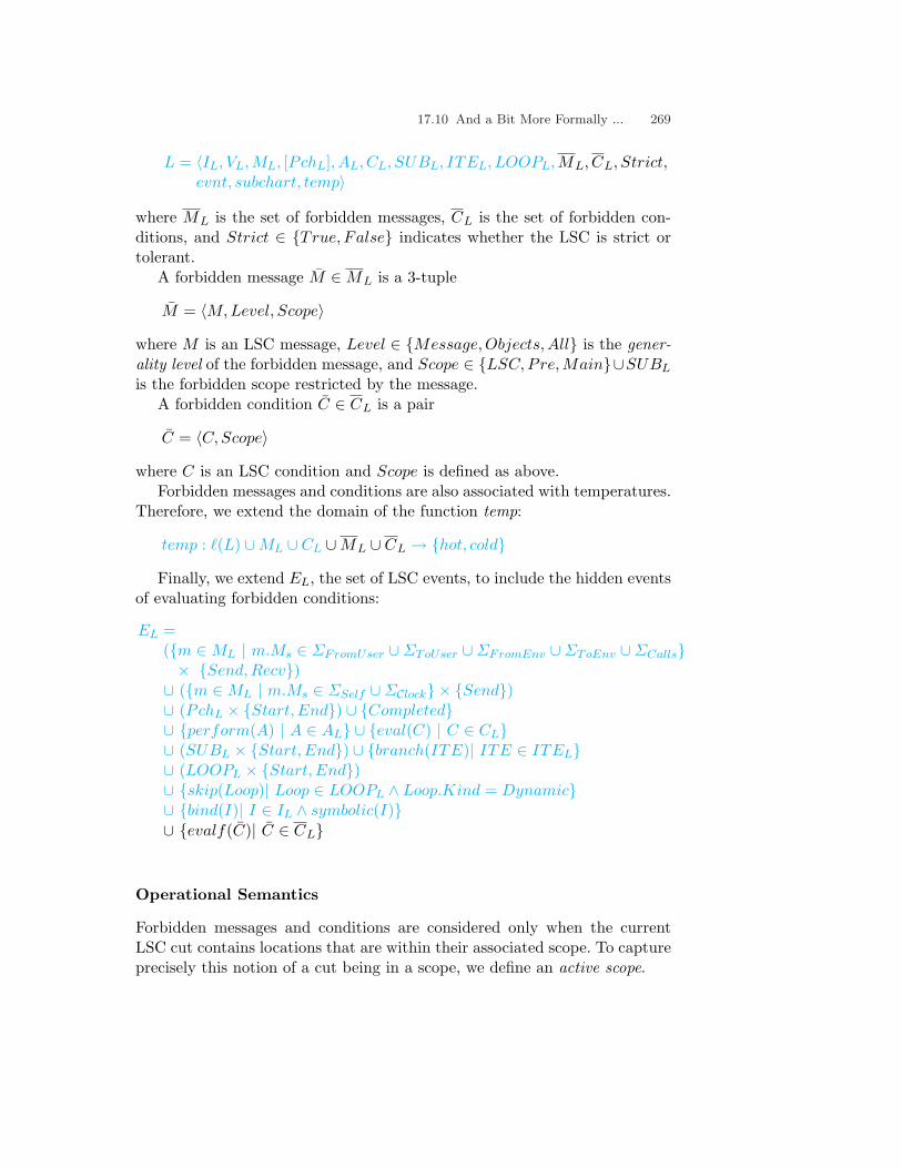
17.10 And a Bit More Formally ... 269
L = 〈IL, VL,ML, [PchL], AL, CL, SUBL, ITEL, LOOPL, ML, CL, Strict,evnt, subchart, temp〉
where ML is the set of forbidden messages, CL is the set of forbidden con-ditions, and Strict ∈ {True, False} indicates whether the LSC is strict ortolerant.
A forbidden message M ∈ ML is a 3-tuple
M = 〈M, Level, Scope〉where M is an LSC message, Level ∈ {Message, Objects, All} is the gener-ality level of the forbidden message, and Scope ∈ {LSC, Pre,Main}∪SUBL
is the forbidden scope restricted by the message.A forbidden condition C ∈ CL is a pair
C = 〈C, Scope〉where C is an LSC condition and Scope is defined as above.
Forbidden messages and conditions are also associated with temperatures.Therefore, we extend the domain of the function temp:
temp : `(L) ∪ML ∪ CL ∪ML ∪ CL → {hot, cold}Finally, we extend EL, the set of LSC events, to include the hidden events
of evaluating forbidden conditions:
EL =({m ∈ ML | m.Ms ∈ ΣFromUser ∪ΣToUser ∪ΣFromEnv ∪ΣToEnv ∪ΣCalls}× {Send, Recv})
∪ ({m ∈ ML | m.Ms ∈ ΣSelf ∪ΣClock} × {Send})∪ (PchL × {Start, End}) ∪ {Completed}∪ {perform(A) | A ∈ AL} ∪ {eval(C) | C ∈ CL}∪ (SUBL × {Start, End}) ∪ {branch(ITE)| ITE ∈ ITEL}∪ (LOOPL × {Start, End})∪ {skip(Loop)| Loop ∈ LOOPL ∧ Loop.Kind = Dynamic}∪ {bind(I)| I ∈ IL ∧ symbolic(I)}∪ {evalf(C)| C ∈ CL}
Operational Semantics
Forbidden messages and conditions are considered only when the currentLSC cut contains locations that are within their associated scope. To captureprecisely this notion of a cut being in a scope, we define an active scope.

270 17. Forbidden Elements
Definition 17.10.1 (active scope). A scope S ∈ {LSC, Pre,Main} ∪SUBL is active in an LSC live copy CL if one of the following holds:
1. S = LSC.2. S = Pre and CL.Mode = PreActive.3. S = Main and CL.Mode ∈ {Active, Check}.4. S ∈ SUBL and ∀I ∈ IS , loc((S, Start)) <L CL.Cut(I) <L loc((S,End)).
Recall that Cut(I) denotes the location of instance I in Cut. Since the startand end of a subchart are synchronization points for all its instances, it issufficient to check any instance in the subchart to see if the subchart is active.We will use the predicate notation active(S) to indicate that a scope S isactive.
We explained in the text that when looking for a violation in the setof forbidden messages we use positive-unification. Moreover, since forbiddenmessages can be in one of several levels of generality, we should define adifferent algorithm for checking whether a forbidden message is unifiablewith a regular one.
Definition 17.10.2 (forbidden message unification). A system messageMs and a forbidden message M are unifiable if one of the following holds:
1. M.Level = All.2. M.Level = Objects and Ms.Src 4 M.M.ISrc ∧ Ms.Dst 4 M.M.IDst.3. M.Level = Message and Ms and M.M are positively-unifiable.
Checking for unification of an LSC message Ml with a forbidden messageM is defined similarly, with Ms.Src and Ms.Dst replaced by Ml.ISrc andMl.IDst, respectively.
Before modifying the transition relation, we define a utility function thatgets as input a set of forbidden messages and returns one of the dominantmessages in the set. A hot message is more dominant than a cold one, and onecold message is more dominant than another if the former’s scope containsthat of the latter. Note that if two forbidden messages are active, their scopesmust be identical or one scope must be contained in the other.

17.10 And a Bit More Formally ... 271
dominant(S)
1. If ∃M ∈ S s.t. temp(M) = hot then return M .2. If all messages are cold then
a) Set M to be any message in S.b) S ← S \ {M}.c) While S 6= ∅ do
i. Choose a message M ′ ∈ S.ii. S ← S \ {M ′}.iii. If M.Scope ⊂ M ′.Scope then set M ← M ′.
d) Return M .
The function dominant is defined in the same way for sets of forbiddenconditions.
The definition of a violating event is now modified, so that events thatappear in an LSC and are not enabled in it are considered violating only ifthe LSC is strict.
Definition 17.10.3 (violating event). An event e violates a chart L in acut C if L.Strict = True and e ∈ ML × {Send, Recv}, but e is not enabledwith respect to C.
The transition relation ∆[SO,SC ] is now modified to handle unification withforbidden messages and to evaluate forbidden conditions. The transition rela-tion assumes that if it is applied to a forbidden condition, the condition holdsand its forbidden scope is active. These assumptions are later guaranteedby the various execution functions, i.e., step, super-step and monitor-event.∆[SO,SC ] is therefore given as:
• If e = 〈M, t〉 (where t ∈ {Send, Recv}) then:1. If e.M.m = Tick then set Clock.T ime ← Clock.T ime + 1.2. Set Context ← ∅.3. If ∃CL ∈ SC and ∃M ∈ CL.LSC.ML, such that e.M and M are unifiable
and active(M.Scope), and there is no enabled event e′ positively level2-unifiable with e, then:
a) Set S ← {M ∈ CL.LSC.ML| Unifiable(e.M, M) ∧ active(M.Scope)}.b) Set M ← dominant(S).c) If temp(M) = hot then
i. Set SC ← SC \ {CL}.ii. Set Violating ← True.
d) If temp(M) = cold theni. If M.Scope ∈ {LSC, Pre,Main} then set SC ← SC \ {CL}.ii. If M.Scope = Sub ∈ SUBL then set

272 17. Forbidden Elements
CL.Cut ← AdvanceCut(CL.Cut, (Sub, End))
4. If ∃CL ∈ SC and ∃e′ ∈ CL.LSC, such that e and e′ are negativelylevel2-unifiable and e′ violates CL, then:
a) Set SC ← SC \ {CL}.b) If temp(CL.Cut) = hot, set Violating ← True.c) If symbolic(e′.M.ISrc) or symbolic(e′.M.IDst) then create an identical
copy C ′L of CL, set SC ← SC ∪ {C ′L}, and in the copy sete′.M.ISrc.Φ ← e′.M.ISrc.Φ ∪ {e.M.Src} if symbolic(e′.M.ISrc)e′.M.IDst.Φ ← e′.M.IDst.Φ ∪ {e.M.Dst} if symbolic(e′.M.IDst)
5. For every universal LSC L ∈ SO which has an event e′, positively level2-unifiable with e, as a minimal event in its prechart, create a copy ofL, CL, and set SC ← SC ∪ {CL}. Set CL.Mode = PreActive and setits cut by CL.Cut ← AdvanceCut(InitialCut(L), 〈PchL, Start〉). Unifythe variables of e and e′, by Unify(e, e′, Context). For each hidden evente′′ <L e′, apply ∆(e′′).
6. For every existential LSC L ∈ SO which has an event e′, positively level2-unifiable with e, as a minimal event in the chart body, create a copy ofL, CL, and set SC ← SC ∪{CL}. Set CL.Mode = Check, and set its cutto the beginning of the chart by CL.Cut ← BeginMainCut(CL.LSC).Unify the variables of e and e′, by Unify(e, e′, Context). For each hiddenevent e′′ <L e′, apply ∆(e′′).
7. For every copy CL ∈ SC that has a reachable event e′ positively level2-unifiable with e:
a) If symbolic(e′.M.ISrc) or symbolic(e′.M.IDst) then create an identicalcopy of CL, C ′L, set SC ← SC ∪ {C ′L}, and in the copy set
e′.M.ISrc.Φ ← e′.M.ISrc.Φ ∪ {e.m.Src} if symbolic(e′.M.ISrc)e′.M.IDst.Φ ← e′.M.IDst.Φ ∪ {e.m.Dst} if symbolic(e′.M.IDst)
b) Set CL.Cut ← AdvanceCut(CL.Cut, e′).c) If e′ = 〈M,Send〉, M is synchronous and e′′ = 〈M, Recv〉,
set CL.Cut ← AdvanceCut(CL.Cut, e′′).d) Unify the events e and e′, Unify(e, e′, Context).e) For each hidden event e′′ <L e′, apply ∆(e′′).
• If e = Completed(CL) for some CL ∈ SC then set SC ← SC \ {CL}.• If e = 〈PchL, End〉 for some CL ∈ SC , then set
CL.Cut ← BeginMainCut(CL.LSC) and CL.Mode ← Active.• If e = perform(A) for some A ∈ AL s.t. CL ∈ SC , then set CL.Cut ←
AdvanceCut(CL.Cut, e) and set

17.10 And a Bit More Formally ... 273
A.V ←
A.C if A.Type = constantV alue(A.P ) if A.Type = propertyA.f(A.λF
f ) if A.Type = function
Clock.T ime if A.Type = time
• If e = eval(C) for some C ∈ CL s.t. CL ∈ SC then1. If value(C) = true then set CL.Cut ← AdvanceCut(CL.Cut, e).2. If value(C) = false then
a) If subchart(C) ∈ {ITE.SubT , ITE.SubE} for some ITE then
set CL.Cut ← AdvanceCut(CL.Cut, (ITE,End))
b) If subchart(C) = Sub ∈ SUBL then
set CL.Cut ← AdvanceCut(CL.Cut, (Sub, End))
c) If subchart(C) = ⊥ then set SC ← SC \ {CL}.d) If temp(C) = hot then set Violating ← True.
• If e = branch(ITE) for some ITE ∈ CL s.t. CL ∈ SC then1. If value(ITE.C) = true then set
CL.Cut ← AdvanceCut(CL.Cut, (ITE.SubT , Start))2. If value(ITE.C) = false then
set CL.Cut ←{
AdvanceCut(CL.Cut, (ITE.SubE , Start)) if ITE.SubE 6= ⊥AdvanceCut(CL.Cut, (ITE.SubT , End)) if ITE.SubE = ⊥
• If e = (ITE.SubT , End) for some ITE ∈ CL s.t. CL ∈ SC then
set CL.Cut ← AdvanceCut(CL.Cut, (ITE,End))
• If e = (ITE.SubE , End) for some ITE ∈ CL s.t. CL ∈ SC then
set CL.Cut ← AdvanceCut(CL.Cut, (ITE.SubE , End))
• If e = (Sub, End) for some Sub ∈ CL s.t. CL ∈ SC then
set CL.Cut ← AdvanceCut(CL.Cut, (Sub, End))
• If e = skip(Loop) for some Loop ∈ CL s.t. CL ∈ SC then
set CL.Cut ← AdvanceCut(CL.Cut, (Loop,End))
• If e = (Loop, Start) for some Loop ∈ CL s.t. CL ∈ SC then
set CL.Cut ← AdvanceCut(CL.Cut, (Loop, Start))
For every variable V ∈ VL that is used in Loop for the first time, setV.ω ← ⊥.

274 17. Forbidden Elements
• If e = (Loop, End) for some Loop ∈ CL s.t. CL ∈ SC and Loop.Kind 6=Dynamic then1. Set µ ← µ− 1.2. If µ > 0 then
set CL.Cut ← AdvanceCut(CL.Cut, (Loop, Start))
For every variable V ∈ VL that is used in Loop for the first time, setV.ω ← ⊥.
3. If µ = 0 then
set CL.Cut ← AdvanceCut(CL.Cut, (Loop,End))
• If e = bind(I) for some symbolic instance I ∈ CLs.t. CL ∈ SC , then:1. S ← {O ∈ O | O 4 I, O satisfies I.ψ and @I ′ ∈ CL s.t. I ′.O = O}.2. If S = ∅ then SC ← SC \ {CL}.3. If I.Mode = Existential then
a) Set I.O = O, for some O ∈ S.b) Set I.C = ⊥.
4. If I.Mode = Universal then perform the following for every O ∈ S:a) Create an identical copy C ′L of CL.b) Set SC ← SC ∪ {C ′L}.c) Set I.O = O.d) Set I.C = ⊥.Finally, set SC ← SC \ {CL}.
• If e = evalf(C) for some C ∈ CL s.t. CL ∈ SC , then (it is guaranteed thatvalue(C) = true)1. If temp(C) = hot then
a) Set SC ← SC \ {CL}.b) Set Violating ← True.
2. If temp(C) = cold thena) If C.Scope ∈ {LSC, Pre, Main} then set SC ← SC \ {CL}.b) If C.Scope = Sub ∈ SUBL then set
CL.Cut ← AdvanceCut(CL.Cut, (Sub, End))
To complete the modifications in the formal semantics caused by forbid-den messages and conditions, we need to modify the procedures super-stepand monitor-event. As opposed to conventional conditions, which are eval-uated according to the partial order induced by the LSC, forbidden condi-tions should affect the course of execution immediately upon becoming true.Therefore, they should be given precedence over other hidden events, both insuper-step and in monitor-event. We begin with the changes in monitor-event:

17.10 And a Bit More Formally ... 275
monitor-event(ev)
1. Apply ∆[SM ,ML](ev).2. Compute the set of forbidden conditions:
Forbidden ←⋃
CL∈ML{C ∈ CL| active(C.Scope) ∧ value(C.C) = true}
3. If Forbidden 6= ∅ thena) C ← dominant(Forbidden).b) Apply ∆[SM ,ML](evalf(C)).c) Go back to 2.
4. Compute the set of enabled events:
Enabled ←⋃
CL∈ML{e ∈ EL|enabled(e)}
Waiting ←⋃
CL∈ML{e | e = branch(ITE)}
∪⋃
CL∈ML{e|e = (Loop, End) ∧ Loop.Kind = Dynamic}
Enabled ← Enabled \Waiting
5. If there is a hidden enabled event e ∈ Enabled, thena) Apply ∆[SM ,ML](e).b) Go back to 2.
6. Terminate monitor-event.
As the Play-Engine selects events to be carried out, it avoids choosingones that are unifiable with active hot forbidden messages, and tries to deferevents that are unifiable with cold forbidden messages. Moreover, it avoidschoosing events that will cause active hot forbidden conditions to becometrue. To capture this behavior formally, we define hot-forbidden events andcold-forbidden events.
Definition 17.10.4 (hot-forbidden event). An event e is hot-forbiddenin a chart L being in a cut C if e is not enabled with respect to C, and if, inaddition, one of the following holds:
• ∃M ∈ ML s.t. active(M.Scope) ∧ temp(M) = hot ∧ Unifiable(e.M, M)• e.M.P 6= ⊥ (i.e., e represents a change in the value of a property) and∃C ∈ CL s.t. temp(C) = hot ∧ active(C) and C will become true if thecurrent value of P is replaced with the value in e.M .

276 17. Forbidden Elements
Definition 17.10.5 (cold-forbidden event). An event e is cold-forbiddenin a chart L being in a cut C if e is not enabled with respect to C and∃M ∈ ML s.t. active(M.Scope) ∧ temp(M) = cold ∧ Unifiable(e.M, M).
We can now continue with the modified super-step:

17.10 And a Bit More Formally ... 277
super-step
1. Compute the set of forbidden conditions:
Forbidden ←⋃
CL∈RL{C ∈ CL | active(C.Scope) ∧ value(C.C) = true}
2. If there is a forbidden condition in Forbidden, thena) C ← dominant(Forbidden).b) Apply ∆[SC ,RL](evalf(C)).c) Go back to 1.
3. Compute the set of enabled events:
Enabled ←⋃
CL∈RL{e ∈ EL|enabled(e)}
Waiting ←⋃
CL ∈ RL,CL.Mode = PreActive
{e | e = branch(ITE)}
Enabled ← Enabled \ (External ∪Waiting)
4. If there is a hidden enabled event e ∈ Enabled, thena) Apply ∆[SC ,RL](e).b) Go back to 1.
5. If there is a visible enabled event e ∈ Enabled, such that e doesnot violate and is neither hot-forbidden nor cold-forbidden in anycopy that is either in active or preactive mode, thena) step(e).b) Go back to 1.
6. If there is a visible enabled event e ∈ Enabled, such that e doesnot violate and is neither hot-forbidden nor cold-forbidden in anycopy that is in active mode, thena) step(e).b) Go back to 1.
7. If there is a visible enabled event e ∈ Enabled, such that e doesnot violate and is not hot-forbidden in any copy that is in activemode with a hot cut, thena) step(e).b) Go back to 1.
8. Terminate super-step.

278 17. Forbidden Elements
17.11 Bibliographic Notes
Forbidden conditions can be used to construct invariants, which are to betrue during the behavior described in an LSC specification. The use of in-variants in programming languages, mainly for capturing the semantics ofloops and for specifying pre-conditions and post-conditions, is one of themost fundamental ideas in program semantics and verification. It was firstproposed by Floyd in [37] and was given a significant push by Hoare’s workin [58].
In the Eiffel programming language [87], invariants are part of the lan-guage itself. They are used to specify pre- and post-conditions for objectmethods, and also to capture class-level invariants, i.e., conditions thatare asserted to hold during the entire life cycle of a class.
In interval temporal logic (ITL) [89, 90], a variant of temporal logicgeared towards expressing properties that hold along specified intervals, onecan specify that a variable has some value during an interval, or that an event,usually indicated by a change in a variable value, is not allowed to happenduring an interval. These capabilities resemble our forbidden conditions andforbidden messages, respectively.

Part VI
Enhancing the Play-Engine


18. Smart Play-Out (with H. Kugler)
In this chapter we provide a brief overview of smart play-out1, a predictivestrengthening of the play-out mechanism, which uses methods from programverification — mainly model-checking.
The chapter should not be viewed as describing another Play-Engine fea-ture, but, rather, as a broader and more recent approach to the very ideaof executing scenario-based requirements. Also, the material described hereis somewhat less complete than that appearing in the rest of the book; forexample, it has not yet been worked out for several features of the LSCs lan-guage. The same applies to the robustness and scope of the implementationof smart play-out, as compared with that of the rest of the Play-Engine. Weexpect to be able to provide a more detailed report on smart play-out in thenear future, as well as a more powerful implementation.
18.1 Introduction
In recent years, formal specification and verification techniques are beginningto be applied to the development of complex reactive systems. Major obsta-cles that still prevent even wider usage of such methods include the factsthat errors are found relatively late in the development process and thathigh expertise is required to correctly capture the properties to be verified.There has been a particular surge in interest in the verification of software-based reactive systems, especially given the success of verification techniquesin hardware development. Due to the size and complexity of such systems,it is desirable to understand all the system requirements, and to make surethey are consistent, before moving on to the implementation phase. In classicverification, a model is first constructed and then verified against well-definedrequirements, whereas one of the main points of this chapter is that verifi-cation techniques can be beneficially applied to the requirements themselvestoo. Alternatively, if one adopts the more ambitious potential of play-in/play-out, leading to systems specified solely in a scenario-based fashion, then smart1 Smart play-out is the central topic of the Ph.D. work of Hillel Kugler (cosupervised by
Amir Pnueli), who is also the main co-author of this chapter.

282 18. Smart Play-Out (with H. Kugler)
play-out can be viewed as utilizing verification techniques to run programsrather than to verify them.
Recall that play-out is actually an iterative process, where after each steptaken by the user the Play-Engine computes a super-step, i.e., a sequenceof events carried out by the system as a response to the event input bythe user. However, the play-out mechanism is, in general, rather naive. Forexample, there can be many possible sequences that are valid responses to auser event, and some of these may not constitute ‘correct’ super-steps. Weconsider a super-step to be correct if when it is executed no active universalchart is violated. By acting blindly by the ‘book’ of requirements, reactingto a user-generated event with the first action it encounters as a possiblereaction to that event, the naive play-out process could very well follow asequence of events that eventually causes violation, even though some othersequence might have been chosen that would have completed successfully. Wewill illustrate this shortly.
From a conceptual point of view, the potential of many possible sequencesof reactions to a user event is due to the fact that LSCs is a declarative,inter-object language, and as such it enables the formulation of high-levelrequirements in pieces (e.g., scenario fragments), leaving open details thatmay depend on the implementation. Technically, the two sources of this non-determinism are the partial order semantics among events in each chart, anddifferent charts containing scenarios that do not have explicit informationabout their interrelationship. These features are very useful in early require-ments stages, but can cause undesired underspecification when one attemptsto execute them. Smart play-out attempts to remove these sources of non-determinism during execution. Thus, depending on whether we view play-in/play-out as a requirements method or an implementation, smart play-outeither ‘helps’ the system fulfil its requirements or strengthens its very execu-tion mechanism.
The smart play-out process uses a powerful program verification tech-nique, called model-checking, to find a ‘correct’ super-step if one exists, andotherwise proving that such a super-step does not exist. In our implementa-tion, the procedure can be applied anew at the occurrence of each user eventin order to examine the different potential super-steps and to find a correctsequence of system reactions if there is one. Once found, the smart play-outmodule feeds this sequence into the Play-Engine, which then executes it tocompletion as a super-step. Model-checking thus drives the execution.
We do not assume that the reader of this chapter is an expert in verifica-tion or model-checking. To get a clear idea of what this chapter describes, itsuffices to know that model-checking is a method by which a desired behav-ioral property of a reactive system is verified over a given system (the model)

18.2 Being Smart Helps 283
through exhaustive enumeration (explicit or implicit) of all the states reach-able by the system and the behaviors that traverse through them. Comparedto other verification approaches, model-checking has two main advantages.First, it is fully automatic, and its application requires no user supervisionor complex mathematical expertise. Second, when the design fails to satisfythe checked-for property, the model-checker is able to produce a counterex-ample that demonstrates some behavior that falsifies the property. In oursmart play-out approach, we make use of these two advantages. Recent yearshave seen intensive research on developing ever-stronger and more efficientmodel-checking algorithms, which renders the approach successful in variousindustrial settings. It also serves to boost our own motivation in seeking waysto make smart play-out more powerful.
18.2 Being Smart Helps
We now use some simple examples to illustrate the role and possible usage ofsmart play-out. Consider the two charts of Fig. 18.1. The first, ‘LSC1’, statesthat when the phone’s cover is opened the display sets its state to show anumber (rather than the current time), the antenna opens and the speakerbecomes silent. It is important to realize that this LSC does not enforce anyparticular order on these three events, since they are relevant to differentobjects. The play-out mechanism will choose one order for execution, in away that is not controllable by the user.
The second chart in the figure, ‘LSC2’, states that whenever the antennaopens, the display should be showing the current time (and this is a hotcondition), it should then set its state to show a number, and only then shouldthe speaker become silent. (The order of these last two events is enforced bythe SYNC condition.)
Assuming that these are the only two specified charts of the system,and that the user opens the cover during play-out, the play-out mechanismchooses the events in an order that results in the charts shown in Fig. 18.2,which describes the situation during the execution. The first event the enginehas chosen to take is the topmost, i.e., setting the display’s state to show anumber. The second is opening the antenna. As this event occurs, ‘LSC2’is activated but cannot progress, since the display shows a number and notthe current time, so the hot condition is false. ‘LSC1’ is also not allowed toprogress, since the event of the speaker turning silent violates ‘LSC2’. There-fore, no progress is allowed at all and the super-step terminates. Note thatthe location of the event of the speaker becoming silent is also hot (denotedby a solid line from that location) so that the entire cut depicted in Fig. 18.2

284 18. Smart Play-Out (with H. Kugler)
Fig. 18.1. Opening the cover of a cellular phone
is also hot. Now, it could be the case that the user decides not to do any-thing else, and, hence, the cut will not progress. This is clearly a violation ofthe requirements, since hot cuts must eventually make progress, and it wascaused by what we call an ‘incorrect’ super-step.
If we apply the smart play-out process to this example, it computes andcarries out a different order of events, as shown in Fig. 18.3. The first eventtaken after the cover is opened is that of opening the antenna. This event ac-tivates ‘LSC2’, but this time the display still shows the current time. The hotcondition is thus evaluated to true and propagated. The display now changesits state to show a number, thus making progress in both charts. Next, thesynchronization condition is successfully passed, and the event of the speakerbecoming silent can be performed, causing the successful completion of bothcharts.
There are situations in which there exists no correct super-step. Consider,for example, the two charts ‘Green First’ and ‘Red First’ in Fig. 18.4. Whenthe user clicks on the PWR button, both charts are activated. However,

18.2 Being Smart Helps 285
Fig. 18.2. Naive play-out
there is no way to satisfy them both since they require the events Changebackground(Green) and Change background(Red) to occur in contradictingorder. Smart play-out proves in this case that no legal super-step exists andannounces this to the user. While this is a very simple example, such con-tradictions can be a lot more subtle, arising as a result of the interactionbetween several charts. In large specifications this can be very hard to ana-lyze manually. The smart play-out framework would prove that in such casesno correct super-step exists.
Another situation in which smart play-out is useful is in detecting theexistence of an infinite loop. Consider the three LSCs of Fig. 18.5. The first,‘LSC1’, states that when the phone’s antenna is opened the reception in thedisplay is set to value 2. The second chart in the figure, ‘LSC2’, states thatwhenever the reception in the display is set to value 2, it should later be setto value 4, while the third chart, ‘LSC3’, requires that setting the receptionin the display to value 4 will later cause the reception value to be set to 2.These three charts together will cause an infinite reaction if the antenna is

286 18. Smart Play-Out (with H. Kugler)
Fig. 18.3. Using smart play-out instead
opened, in which ‘LSC2’ and ‘LSC3’ repetitively activate each other. Theplay-out mechanism would indeed execute this ‘infinite loop’ while smartplay-out will detect this situation and notify the user.
Smart play-out can be used to satisfy existential charts. As discussedearlier, existential LSCs may be used to specify system tests. Smart play-outcan then be used to find a trace that satisfies the chart without violatinguniversal charts on the way. Figure 18.6 shows a test, in which user andexternal environment actions are performed and expected system responsesare described using conditions. In this chart, the user opens the cover andenters the number 4050. In response, the display is expected to show thedialed number. Next, the user clicks the ‘SEND’ button and the phone’sspeaker is expected to ring. Finally, when a signal from the environmentindicating the acceptance of the call (denoted by the “ACK” reserved word)is received by the phone’s chip, the speaker turns silent. Smart play-outfinds a trace satisfying the chart and all the activated universal charts and

18.3 The General Approach 287
Fig. 18.4. Inconsistent LSCs
the execution is then shown by the Play-Engine. More information on usingsmart-play to satisfy existential charts can be found in Sect. 18.6.
18.3 The General Approach
The approach we use is to formulate the play-out task as a verification prob-lem, and to use the counterexample provided by a model-checking algorithmas the desired super-step. The system on which we perform model-checkingis constructed according to the universal charts in the LSC specification. Wedefine a transition relation from the LSC specification, which is designed toallow progress of active universal charts but prevents any violations. Thesystem is initialized to reflect the status of the application just after the lastexternal event occurred, including the current values of object properties, in-formation on the universal charts that were activated as a result of the mostrecent external events, and the progress in all precharts.
The model-checker is then given a property claiming that always (in thetemporal sense) at least one of the universal charts is active. In order to

288 18. Smart Play-Out (with H. Kugler)
Fig. 18.5. Infinite loop
falsify the property, the model-checker searches for a run in which eventuallynone of the universal charts is active, i.e., all active universal charts completesuccessfully, and, by the definition of the transition relation, no violationsoccurred in the process. Such a counterexample is exactly the desired super-step. If the model-checker verifies the property then no correct super-stepexists. The next section provides details on how we construct the input tothe model checker.
It is important to note that smart play-out (at least as it stands when thiswas written — February 2003) does not backtrack over super-steps. Thus, wemay get to a situation where no correct super-step exists due to moves thesystem made in previous super-steps, which could perhaps have been donedifferently. This demonstrates the difference between smart play-out, whichlooks one super-step ahead, and full synthesis, which performs a completeanalysis. Moreover, currently smart play-out is limited to a rather restrictedversion of the LSCs language, as we discuss later.
It should also be emphasized that from a computational complexity pointof view smart play-out, being based on model-checking, is more problem-atic then naive play-out. First, model-checking is in general undecidable forinfinite-state systems. Second, even for finite-state systems, the time complex-

18.4 The Translation 289
Fig. 18.6. Smart play-out satisfying an existential chart
ity of the problem turns its application to real-world systems into a majorchallenge.
Having said all this, our goal in future research on smart play-out is toextend the subset of LSCs that is supported and to improve the efficiencyof the algorithms. We shall address several aspects of this in the remainingparts of the chapter.
18.4 The Translation
A formal definition of the operational semantics of LSCs as implemented inthe Play-Engine appears in Appendix A. Central to the semantics is a sym-bolic transition system, where the states are the set of LSC copies (whichcontain cuts that specify progress), and LSC events correspond to the tran-sitions. The transition system is then used to define the play-out executionmechanism. Roughly speaking, play-out selects an enabled event that doesnot cause a violation in any of the universal LSC copies and executes it, it-erating this process until no such enabled events exist. If, at a certain stagein the super-step, there are several enabled events, the play-out mechanismchooses one of them in an uncontrollable way that is a function of the con-crete implementation of the Play-Engine and the particular LSC specificationexecuted. No special effort is made to prefer a certain event over another. The

290 18. Smart Play-Out (with H. Kugler)
choice is purely ‘local’, and does not take into account the effects this mayhave down the line.
Smart play-out uses model-checking algorithms to make a ‘global’ deci-sion on the super-step level. The technique takes into account the effects ofchoosing a particular enabled event, and makes the actual choice in a waythat guarantees successful completion of the super-step, if possible.
Our main focus is to search for a correct behavior of the system whenseveral charts act together. Accordingly, we construct a transition systemwith one process for each actual object. A state in this system indicates thecurrently active charts and the location of each object therein. The transitionrelation restricts the transitions of each process to moves that are allowed byall the currently active charts. Note that our translation does not explicitlyconstruct the cuts for each chart (which by itself causes an exponential growthin the size of the initial representation).
We now provide more details on how to translate a play-out problem intoa model-checking problem. In the rest of this section, we use terms that weredefined in the more formal sections of the book.
An LSC specification S = SU ∪ SE consists of a set of charts, where eachchart m ∈ S is existential or universal. We denote by pch(m) the prechart ofchart m. Assume that the set of universal charts in S is SU = {m1,m2, ...,mt},and that the objects participating in the specification are O = {O1, ..., On}.
We define a transition system with the following variables:
actmi – determining if universal chart mi is active. Its value is 1 when mi isactive and 0 otherwise.
msgsOj→Ok
– denoting the sending of message msg from object Oj to objectOk. Its value is set to 1 at the occurrence of the send and is changed to0 at the next state.
msgrOj→Ok
– denoting the receipt by object Ok of message msg sent by objectOj . Its value is set to 1 at the occurrence of the receive and is changedto 0 at the next state.
lmi,Oj – denoting the location of object Oj in chart mi. It ranges over0 · · · lmax, where lmax is the last location of Oj in mi.
lpch(mi),Oj– denoting the location of object Oj in the prechart of mi. It ranges
over 0 · · · lmax, where lmax is the last location of Oj in pch(mi).
Throughout this chapter, we assume the asynchronous mode of messages,in which a send and a receive are separate events; however, smart play-out supports the synchronous mode too. We denote by f(l) = evnt(l) theevent associated with location l, and use the convention that primed variablesdenote the value of a variable in the next state, while unprimed variablesrelate to the current state.

18.4 The Translation 291
The following subsections show the definition of the transition relation,organized by the various features of the LSC language.
Messages
We first define the transition relation for the location variable when thelocation corresponds to the sending of a message:
l′mi,Oj=
{l if lmi,Oj = l − 1 ∧msgs
Oj→Ok
′ = 1l − 1 if lmi,Oj = l − 1 ∧msgs
Oj→Ok
′ = 0
Intuitively, if object Oj is at location l−1 in chart mi, and the next locationof Oj corresponds to the sending of message msg from Oj to Ok, then if in thenext state the message is sent, the location is advanced; otherwise it remainswhere it is. It is important to notice that the event msgs
Oj→Okmay not be
allowed to occur at the next state due to the happenings in some other chart.This is one of the places where the interaction between the different chartsbecomes important.
As for the receipt of events, given that n is the location in which messagemsg is sent from object Oj to object Ok in mi, we define the transitionrelation as:
l′mi,Ok=
{l if lmi,Ok
= l − 1 ∧ lmi,Oj ≥ n ∧msgrOj→Ok
′ = 1l − 1 if lmi,Ok
= l − 1 ∧ (lmi,Oj < n ∨msgrOj→Ok
′ = 0)
If object Ok is at location l − 1 in chart mi, and the next location ofOk corresponds to the receipt of the message msg sent by object Oj , andthis message has already been sent, then if in the next state the message isreceived, the location is advanced; otherwise it remains where it is.
We now define the transition relation for the variable that determines theoccurrence of a send event (the receive case is similar):
msgsOj→Ok
′ ={
1 if φ1 ∧ φ2
0 otherwise
φ1 ,∨
mi∈SU∧msgsOj→Ok
∈Messages(mi)
actmi = 1
φ2 ,∧
mi∈SU∧msgsOj→Ok
∈Messages(mi)
(actmi = 0 ∨ ψ(mi))
ψ(mi) ,∨
lt s.t. f(lt)=msgsOj→Ok
(lmi,Oj = lt − 1 ∧ l′mi,Oj= lt)

292 18. Smart Play-Out (with H. Kugler)
Let us explain. In order for the event of sending msg from Oj to Ok to oc-cur, we require two conditions to hold, which are expressed by the formulas φ1
and φ2, respectively. The first, φ1, states that at least one of the main chartsin which this message appears is active. The assumption is that message com-munication is caused by universal charts that are active and does not occurspontaneously. The second requirement, φ2, states that all active charts must‘agree’ on the message. For an active chart mi that contains msgs
Oj→Ok, we
require that object Oj progresses to a location lt corresponding to this mes-sage, as expressed by the formula ψ(mi). Formula φ2 states that for all chartsmi containing msgs
Oj→Ok(that is, msgs
Oj→Ok∈ Messages(mi)), either the
chart is not active or the message can occur (that is, ψ(mi) holds). Accordingto the semantics of LSCs, if a message does not appear in a chart explicitly,it (i.e., its sending and receipt) is allowed to occur between the messages thatdo appear, without violating the chart. This is reflected in φ2 by the fact thatthe conjunction is only over the charts containing msgs
Oj→Ok.
Precharts
The prechart of a universal chart describes the scenario which, if completedsuccessfully, forces the scenario described in the main chart to occur. Themain chart becomes active if all locations of the prechart have reached max-imal positions, which is what successful completion of the prechart means.A central feature of play-out is that a sequence of events in a super-stepmay cause the activation of some additional universal chart, which now mustalso be completed successfully as part of the same super-step. For this pur-pose precharts are monitored, and locations along instance lines are advancedwhen messages are sent and received.
The transition relation for a location variable in a prechart is similar tothe one defined for locations in the main chart, with one major difference:precharts are allowed to be violated. If a message is sent or received while it isnot enabled in the prechart, the prechart is ‘reset’ by moving all its instancesback to their initial locations. This reset action allows the prechart to start‘looking’ for another way to be satisfied. In fact, when the model-checkersearches for a ‘correct’ super-step it often tries to violate a prechart in ordernot to get into the obligation of having to satisfy the corresponding mainchart. When all locations in the prechart reach their maximal positions, theytoo are reset.
Formally, if the prechart location is lpch(mi),Oj= l − 1, and the next
location corresponds to a message sending, then its transition relation isgiven by:

18.4 The Translation 293
l′pch(mi),Oj=
l if msgsOj→Ok
′ = 10 if msgs
Oj→Ok
′ = 0 ∧ Φ(mi)l − 1 otherwise
Φ(mi) ,∨
msgsOx→Oy
∈Messages(mi)
Ψ s(msgsOx→Oy
)
∨∨
msgrOx→Oy
∈Messages(mi)
Ψ r(msgrOx→Oy
)
∨∧
Oj∈Obj(mi)
(lpch(mi),Oj= lmax
pch(mi),Oj)
Ψ s(msgsOx→Oy
) ,
1 if lmi,Ox = lx − 1 ∧ f(lx) 6= msgsOx→Oy
∧msgs
Ox→Oy
′ = 10 otherwise
Ψ r(msgrOx→Oy
) ,
1 if lmi,Oy = ly − 1 ∧ f(ly) 6= msgrOx→Oy
∧msgr
Ox→Oy
′ = 10 otherwise
Ψ s (respectively, Ψ r) checks whether a send (respectively, receive) event oc-curred while not enabled by its sender (respectively, receiver) instance inthe chart. Φ(mi) checks whether all locations have reached their maximalposition.
Activation of Charts
For a universal chart mi, we define the transition relation for actmi as follows:
act′mi=
1 if φ(pch(mi))0 if φ(mi)actmi otherwise
φ(mi) ,∧
Oj∈Obj(mi)
(l′mi,Oj= lmax
mi,Oj)
The main chart mi becomes active when all locations of the prechart reachmaximal positions, and it stops being active when all locations of the mainchart reach maximal positions.
Object Properties and Conditions
Although the basic strength of scenario-based languages like LSCs is in show-ing message communication, the LSC language has the ability to reason about

294 18. Smart Play-Out (with H. Kugler)
the properties of objects too. Object properties can be referenced in conditionconstructs, and these can be hot or cold. According to the semantics of LSCs,if a cold condition is true the chart progresses to the location that immedi-ately follows the condition, whereas if it is false the surrounding (sub)chartis exited. A hot condition, on the other hand, must always be met, otherwisethe requirements are violated and the system aborts. To support this kind ofreasoning, we have to update the value of each property as the system runs.
More formally, let P tOk
denote the tth property of object Ok, defined overa finite domain D. For many of the object properties there are simple rules— defined when the application and the GUI are constructed — that relatethe value of the property to message communication. Accordingly, supposethat message msg received by Ok from Oj has the effect of changing propertyP t of object Ok to the value d ∈ D. We then add to the transition relationof process Oj the clause
P tOk
′ = d if msgrOj→Ok
′ = 1
In this way, the values of the properties are updated as the objects sendand receive messages.
Object properties can be referred to in conditions. In fact, we take acondition expression to be a Boolean function over the domains of the objectproperties, C : D1 ×D2 × · · · ×Dr → {0, 1}, so that a condition can relateto the properties of several objects. Here, the properties appearing in thecondition are P1, P2, . . . , Pr.
A condition affects the transition relation of the location of a participatingobject. Here is how we deal with a hot condition: To simplify the presentationof the definition, we assume only two objects participating in the condition.In the general case, of course, there could be a single object or many objects.If object Oj is at location lj − 1 and object Ok is at location lk − 1 in chartmi, and if their next locations correspond to the hot condition C, we define:
l′mi,Oj=
{lj if C(dj , dk)′ = 1 ∧ lmi,Oj = lj − 1 ∧ lmi,Ok
= lk − 1lj − 1 if lmi,Oj = lj − 1 ∧ ((C(dj , dk)′ = 0 ∨ lmi,Ok
6= lk − 1)
Object Oj moves to location lj if both objects participating in the con-dition are ready for the evaluation of the condition expression, being at lo-cations lj − 1 and lk − 1, respectively, and the condition C holds. Here, dj
and dk are the values of properties P sOj
and P tOk
, respectively. The transi-tion relation thus ensures synchronization of the objects when evaluating thecondition and allows progress only if the condition expression holds, thuspreventing violation of the chart. In this definition, we assume that there are

18.4 The Translation 295
two objects, Oj and Ok, constrained by the condition, whereas, as mentioned,in the general case there could be a single object or several.
For a cold condition we define:
l′mi,Oj=
lj if C(dj , dk)′ = 1 ∧ lmi,Oj = lj − 1 ∧ lmi,Ok= lk − 1
ls if C(dj , dk)′ = 0 ∧ lmi,Oj = lj − 1 ∧ lmi,Ok= lk − 1
lj − 1 if lmi,Oj = lj − 1 ∧ lmi,Ok6= lk − 1
The difference between this and the previous definition for a hot conditionis that here, if the objects are ready for the evaluation of the condition butthe condition does not hold, the smallest surrounding (sub)chart is exited,as per the semantics of LSCs. Here, ls is the location of object Oj at the endof the surrounding (sub)chart. In such a case, all the other objects will alsosynchronize their exit of this (sub)chart. Note that this is a ‘peaceful exit’,and it does not constitute a violation of the universal chart mi.
Assignments
Among other things, assignments enable us to refer to system propertiesafter they are set. In the assignment x := d, the value d may be a constant,a property value of some object, or the value obtained by applying somefunction to other values. To handle assignments we add to our translation aBoolean variable assign(x, d) that is set to 1 exactly when the assignment isperformed. Actually, these variables are used only for notational clarity, sincein the implementation they can be computed from the values of the locationvariables. The translation is straightforward:
x′ ={
d if lmi,Ok= l − 1 ∧ l′mi,Ok
= l ∧ assign(x, d)x otherwise
Intuitively, if object Ok is at location l − 1 in chart mi, and the nextlocation of Ok corresponds to the assignment x := d, the value of x is set tod.
We also add to the system a Boolean variable xbound, which determineswhether variable x is already bound to a concrete value. After an assignmentis evaluated, xbound is set to 1. More information about this appears in the“Symbolic Messages” subsection below.
Assignments are local to a chart. Typically, the variable x on the left-handside of the assignment will be used later in the chart, as part of a conditionor a symbolic message.

296 18. Smart Play-Out (with H. Kugler)
Symbolic Messages
A symbolic message is of the form msg(x), where x is a parameter rangingover a finite domain D. (Actually, a message can have more than one variable,but for clarity we explain the simple case of a single variable.) It representsconcrete messages of the form msg(d), where d ∈ D. Using symbolic messagesit is possible to describe generic scenarios, which are typically instantiatedand bound to concrete values during play-out.
To handle msg(x) in smart play-out, we add a variable representing theparameter x, which can be bound to a concrete value as the result of the oc-currence of a concrete message or an assignment. The binding of this variablealso affects other messages in the same chart that are parameterized by x,binding them to the same value. Once the variables of a symbolic message arebound to concrete values, the usual rules concerning message communicationapply to it, so that the message will affect the transition relation in a waysimilar to that of a regular message.
Formally, for a symbolic message of the form msg(x) we add a variablex ∈ D and a Boolean variable xbound that determines whether variable x isalready bound to a concrete value. Initially, we set xbound to 0, and we definethe transition relation as follows:
x′bound ={
1 if φ1 ∨ φ2 ∨ xbound = 10 otherwise
φ1 , lmi,Oj = l − 1 ∧ l′mi,Oj= l ∧
∨
d∈D
msg(d)′ = 1
φ2 ,∨
lt s.t. f(lt)=assign(x)
(lmi,Ok= lt − 1 ∧ l′mi,Ok
= lt)
Thus, xbound is changed to 1 if the concrete message msg(d) occurs, withd ∈ D (as defined by φ1), or when x appears in the left-hand side of anassignment that is being evaluated (as defined by φ2).
The transition relation for the variable x is defined as follows:
x′ ={
d if lmi,Oj = l − 1 ∧ l′mi,Oj= l ∧ (msg(d)′ = 1 ∨ assign(x, d)′ = 1)
x otherwise
The first case corresponds to the binding of x to the value d, as the resultof the occurrence of the concrete message msg(d) or as the result of x beingassigned the value d. Otherwise, x remains unchanged.

18.4 The Translation 297
We now define the transition relation for the location variable when thelocation corresponds to a symbolic message:
l′mi,Oj=
{l if lmi,Oj = l − 1 ∧∨
d∈D (msg(d)′ = 1 ∧ x′bound = 1 ∧ x′ = d)l − 1 if lmi,Oj = l − 1 ∧∧
d∈D (msg(d)′ = 0 ∨ x′bound = 0 ∨ x′ 6= d)
Intuitively, if object Oj is at location l−1 in chart mi, and the next locationof Oj corresponds to a symbolic message, then the location is advanced if themessage msg(d) occurs and x is bound to the value d ∈ D.
If-Then-Else
The transition relation of the if-then-else construct is a variation on theway conditions are handled earlier. All participating objects are synchronizedwhen the condition is evaluated and when entering and exiting the ‘then’ and‘else’ parts.
l′mi,Oj=
lj if C(dj , dk)′ = 1 ∧ lmi,Oj = lj − 1 ∧ lmi,Ok= lk − 1
lej if C(dj , dk)′ = 0 ∧ lmi,Oj = lj − 1 ∧ lmi,Ok= lk − 1
lj − 1 if lmi,Oj = lj − 1 ∧ lmi,Ok6= lk − 1
lej − 1 if lmi,Oj = lej − 1 ∧ lmi,Ok6= lek − 1
lxj if (lmi,Oj = lxj − 1 ∧ lmi,Ok6= lxk − 1)
∨ (lmi,Oj = lej − 1 ∧ lmi,Ok= lek − 1)
Here, lej and lek are the locations of objects Oj and Ok at the beginning ofthe else subchart, and lxj and lxk are the locations of these objects at the endof the else subchart, respectively.
Loops
A loop is a sub-chart whose behavior is iterated, and all objects are synchro-nized at the beginning and end of each iteration. Loops can be of two basictypes, bounded or unbounded; see Chap. 13. The transition relation shouldsynchronize the objects at the beginning and end of each iteration, and forthe bounded case a counter variable is added to ensure that the given boundis not exceeded.
To simplify the presentation of the definition, we assume that there areonly two objects participating in the loop, Oj and Ok, and that they end theloop at locations lej and lek, respectively. (In the general case, of course, therecould be a single object or many objects.)

298 18. Smart Play-Out (with H. Kugler)
For the bounded case, where the loop is iterated N times, and where lejis the first location of object Oj after the loop and lbj is the first location ofOj inside the loop, we add a loop variable x, initialized to 1, and add thefollowing conjunct to the transition relation:
l′mi,Oj=
{lej if x = N ∧ lmi,Oj = lej − 1 ∧ lmi,Ok
= lek − 1lbj if x < N ∧ lmi,Oj = lej − 1 ∧ lmi,Ok
= lek − 1
x′ ={
x + 1 if x < N ∧ lmi,Oj = lej − 1 ∧ lmi,Ok= lek − 1
1 if x = N ∧ lmi,Oj = lej − 1 ∧ lmi,Ok= lek − 1
Intuitively, if the objects do not exit the loop by the variable x reachingthe required number of iterations N , they reiterate the loop (object Oj movesto its loop start location lbj). The transition relation synchronizes the objectsat the beginning and end of each iteration. The loop variable x is incrementedin each iteration of the loop.
For an unbounded loop we do not add a loop variable, and the transitionrelation is defined as follows:
l′mi,Oj= lb if lmi,Oj = lj − 1 ∧ lmi,Ok
= lk − 1
When they reach the end of the loop the objects always change locationsto their start loop ones. The loop can be exited by a cold condition beingevaluated to false inside the loop, as explained earlier.
The Model-Checking Formula
To compute a super-step in the execution of an LSC system using a modelchecker, the system is initialized according to the current locations of in-stances in precharts, while all locations in the main charts are set to 0. Themain chart’s activation state is also initialized to reflect the current state. Af-ter each external event, the Play-Engine decides which precharts have com-pleted and sets their corresponding main charts to be active. We also set theproperties of the objects to reflect their current value.
The model checker is then given the following property to prove, statingthat it is always the case that at least one of the universal charts is active:
G(∨
mi∈SU(actmi = 1))
As explained earlier, falsifying this property amounts to finding a runthat leads to a point at which all active universal charts have completedsuccessfully, with no violations — which is exactly the desired super-step.

18.5 Current Limitations 299
18.5 Current Limitations
Features Not Covered
Smart play-out, being based on model-checking, cannot support the LSClanguage in full. We now briefly discuss those LSC features that are eithernot supported yet or are supported only in part. Some of these we believe weknow how to handle, but have not yet worked out the details.
String variables: Model checkers can handle only finite-state systems. Inthe Play-Engine all types are indeed finite, although using a string type witha large maximal length would make model-checking infeasible in practice.In our current implementation of smart play-out, string variables are notsupported. In the future we intend to use abstractions, either automatic orproposed by an advanced user, to enable smart play-out to handle strings orinfinite types.
Dynamic loops: We explained earlier how smart play-out handles fixedloops and unbounded loops. A third type of loop is the dynamic loop, inwhich the user determines the number of times the loop is iterated. How toperform this interaction with the user while in smart play-out and how tohandle some of the subtle semantic issues regarding dynamic loops requirefurther research.
External objects: When the chart body contains interactions with enti-ties that are external to the system — the user, environment, external objectsor time — we cannot guarantee that all maximal positions are reached withina single super-step, because play-out cannot initiate moves that are not madeby the system. Currently smart play-out has limitations in handling these sit-uations and we are working on trying to overcome them.
Multiple active copies of a chart: In order to identify the activationof a universal chart it is sometimes necessary to maintain several copies ofthe same prechart, each one in a different stage of the prechart’s scenario.A universal chart may also be reactivated before its main chart completes,causing several copies of the main chart to be active simultaneously. In theabsence of unbounded loops, the maximal number of simultaneously activecharts and precharts is bounded and can be easily computed. Actually, wepredict that in most practical cases these bounds will be small, because inorder for the bound to be large there must be a very strong correlationbetween the messages in the prechart and the main chart, and this is usuallynot the case. In any case, we have not yet dealt with multiple active copiesof the same chart.
Implemented functions: As explained in Sect. 18.4, message communi-cation can have an effect on the values of object properties. If there is a simple

300 18. Smart Play-Out (with H. Kugler)
rule relating the value of a property to message communication, this can befully handled in the transition relation. In cases where implemented functionsare used, the situation is more complicated. We plan to investigate severaldirections in trying to deal with implemented functions in smart play-out.Currently we use a practical approach, creating a symbolic trace of eventsthat is bound to actual values at a later stage, iteratively. This approach,however, is not guaranteed to produce a correct super-step; in such cases theproblem will be indicated during execution of the super-step.
Probabilistic nondeterminism: Smart play-out handles probabilisticnondeterministic choices without taking into account the probabilities. Thenondeterminism is directly reflected in the transition relation, and smartplay-out can thus consider all possible choices when searching for a satisfyingrun. Future research directions may include taking into account the proba-bilities obtained by analyzing the probability of a satisfying run, or finding asatisfying run with the highest probability, etc. Recent work on probabilisticverification and probabilistic model-checking may be relevant here too.
Classes and symbolic instances: Extending live sequence charts tohandle symbolic instances enhances the expressive power of the LSC languageand thus makes smart play-out a harder challenge. For the general case inwhich the number of objects is not bounded the problem is undecidable. Thecurrent Play-Engine implementation does not allow dynamic creation anddestruction of objects, so that their number is fixed per specification. Evenso, applying the smart play-out idea to specifications with symbolic instancesis a difficult challenge, which we are currently investigating.
Time: Extending LSCs with time can introduce undecidability resultswhen attempting to apply smart play-out. Our work focuses on characterizinginteresting cases in which smart play-out can be performed, and handlingthem efficiently. Another research direction is dealing with continuous timeinstead of the discrete time approach used in the Play-Engine.
Forbidden elements: The use of forbidden elements is another recentextension of LSCs, which is not yet covered in the smart play-out. We believethat it does not present new fundamental limitations, and hope to work outthe details soon.
The Semantics of Smart Play-Out
Although we have made an effort to base play-out and smart play-out on thesame LSC semantics, there are still some small differences, for a number ofreasons. One reason is that play-out implements ‘violation policies’, i.e., itfirst tries to find an event that does not violate a prechart and only if that isimpossible does it choose a violating event. In contrast, smart play-out does

18.6 Satisfying Existential Charts 301
not implement such policies and ‘cares’ only about finding a correct super-step. This difference, however, is not an inherent limitation, and in the futurewe may consider adding information to the smart play-out process that willallow it to implement different violation policies.
A similar difference is that smart play-out sometimes allows more nonde-terminism — for example, in deciding when a certain LSC construct shouldbe evaluated. There are some cases (e.g., assignments) in which we believethis freedom is not necessary and we plan to modify our translation schemeto capture the same semantics as in the standard play-out. There are situ-ations, however, in which the smart play-out approach has the potential tocapture a more realistic and convenient semantics, such as in certain cases ofevaluating conditions and in determining exactly when a prechart has beenactivated. We plan to further investigate these possibilities, while gainingmore experience in using LSCs for more realistic examples.
18.6 Satisfying Existential Charts
An additional powerful way to utilize the techniques we have developed forcalculating a super-step is in satisfying an existential LSC. Here the smartplay-out approach enhances the Play-Engine’s capabilities by automaticallyfinding a satisfying run for a given existential chart. To do this using onlythe standard play-out we would have to designate the existential LSC as amonitored chart, and then run play-out as we see fit, trying on our own tocause the chart to be traced to completion.
In this section we briefly describe some of the ways in which smart play-out provides extended analysis capabilities for satisfying existential charts.We illustrate the ideas using a biological model of the development of partsof the egg-laying system of the nematode Caenorhabditis elegans, fondlycalled C. elegans by the research community.
Satisfying from Any Configuration
When formulating a play-out task as a verification problem, the system mustbe initialized to reflect the status of the application, in particular, the currentvalues of all object properties. For the purpose of using smart play-out forsatisfying existential charts, it is often useful to relax this constraint andallow the setting of a more general initial configuration.
Consider the C. elegans model whose GUI appears in Fig. 18.7. The GUIcontains elements representing simplified versions of the worm’s gonad, in-cluding its anchor cell (AC), and the six vulval precursor cells (VPCs). During

302 18. Smart Play-Out (with H. Kugler)
Fig. 18.7. GUI for part of the egg-laying system of C. elegans
normal development, three of the six VPCs are induced by the AC to executevulval (primary or secondary) fates. Induced cells go through three roundsof cell division, resulting in 22 cells that form the worm’s vulva. Uninducedcells adopt a tertiary (non-vulva) fate, and divide only once. The GUI in thefigure represents the developmental decisions that occur during a discretewindow of time, and it was constructed to directly reflect the way biologistsrepresent the relevant part of the anatomy of C. elegans. Its form is naturaland clear for anyone working on C. elegans vulval development.
The general behavioral scheme of our C. elegans model is that during theexperimental setup the user can perform various genetic manipulations andcell ablations. After this setup stage, the development starts (captured duringthe modeling by clicking the Start button), and the egg-laying subsystemevolves; the different cells communicate and adopt different fates. The be-havior is strongly dependent on the types of mutations that occurred at theinitial stages.
This is consistent with the relevant biological data obtained from C. ele-gans researchers. Large parts of this data are of the ‘condition-result’ kind,and are usually gathered in an experiment triggered by a certain set of circum-stances (conditions), following which an observation is made and the resultsrecorded. The condition is often a set of perturbations, such as mutatinggenes or exposing cells to an altered environment. Another example includesobservations of the effects of anatomical manipulations (e.g., cell destructionor tissue transplantation) on the behavior of the remaining structures. Tomodel such condition-result experiments, the prechart of the LSC is playedin to represent the experimental setup (i.e., the alterations that were intro-

18.6 Satisfying Existential Charts 303
duced to the biological system), and the main chart captures the observedbehavior (e.g., cell fates adopted during development). Thus, most of theinteractions between experimentalists and the biological system they inves-tigate, and therefore also between them and our biological model, involvemodifications to the initial configuration of the system.
As an example, consider the task of satisfying the existential chart ofFig. 18.8, which states that some time after the system starts development,the P7.p cell adopts a tertiary fate, which shows up in the GUI by the cellbeing colored yellow. We instruct the smart play-out module to find a way to
Fig. 18.8. Cell P7.p adopts a tertiary fate
initialize the system with some combination of mutations and cell ablations,which leads to the chart being satisfied. This corresponds to trying to findthe experimental conditions that lead to the desired result. If the systemsucceeds, it informs the user of the initial configuration that it used to satisfythe chart, as shown in Fig. 18.9. Notice the mutation of dig-1, which enables
Fig. 18.9. Notifying the user of the initial configuration used
the scenario of ‘displacement of the gonad’ to be activated, as described inFig. 18.10, and leads P7.p to adopt a tertiary fate, as desired.

304 18. Smart Play-Out (with H. Kugler)
Fig. 18.10. Displacing the gonad (DIG) mutation
Finding Different Satisfying Runs
When using smart play-out to satisfy an existential LSC, it can be veryhelpful to obtain not only a single satisfying run but many such runs, if theyexist. Our experience in the work on C. elegans showed that in certain casesthe fact that there is a way to satisfy a given existential chart did not comeas a surprise to the biology experts. However, they were often surprised bythe different ways of satisfying it, sometimes by scenarios that they initiallydid not think were relevant.
To make it possible to find a number of satisfying runs within the smartplay-out framework, the Play-Engine can be instructed to record a satisfy-ing run and to transform it automatically into an anti-scenario. Figure 18.11

18.6 Satisfying Existential Charts 305
shows the anti-scenario obtained from the satisfying run of the ‘Dig’ scenariodiscussed above. We can now add this anti-scenario to the LSC specification
Fig. 18.11. Automatically generated anti-scenario for the DIG mutation
and go back to the smart play-out procedure, asking it again to satisfy theoriginal existential chart. However, now it does so after enriching the spec-ification with the new anti-scenario, so that the first solution will not bedetected, since the first satisfying scenario is now forbidden. Indeed, a differ-ent satisfying run is found, which starts with the ‘loss-of-function’ mutation(lof) of the let-23 gene, resulting in a vulvaless phenotype: all six VPC cells,and in particular P7.p, adopt a tertiary fate. See Figs. 18.12 and 18.13.
Fig. 18.12. Another way for P7.p to become tertiary

306 18. Smart Play-Out (with H. Kugler)
Fig. 18.13. The vulvaless scenario

18.7 Bibliographic Notes 307
18.7 Bibliographic Notes
Smart play-out was first described in [47], and is the central topic of thePh.D. work of H. Kugler. For a survey on model checking, with a wealth ofinformation, see [22].
Preliminary results on using LSCs for the modeling and analysis of C. ele-gans development appear in [63], and are the central topic of the Ph.D. workof N. Kam. This recent modeling and analysis project helped inspire some ofthe features described in Sect. 18.6. For further information about C. elegansvulva development, see [38, 79].


19. Inside and Outside the Play-Engine
In this chapter, we give a brief overview of the Play-Engine’s architecture, andprovide schematic descriptions of the way it handles its two main functions,play-in and play-out.
19.1 The Engine’s Environment
Figure 19.1 shows the main components that participate in the play-in andplay-out processes, and how the Play-Engine itself fits in. The top cloud rep-resents the various graphical user interfaces that can be used for playing inand playing out. Among other things, they include mock-ups of electronicdevices, dialogs and forms used in software systems, object model diagrams,etc. The Application Interface is implemented by any GUI application thatwants to interact with the Play-Engine. It is used by the engine to instructthe GUI application to perform various commands, such as changing valuesof properties, highlighting objects, etc. The Play-Engine Interface is imple-mented by the Play-Engine, and is used by the GUI application to notify thePlay-Engine of various events, such as right-clicking on an object or changinga property’s value (e.g., flipping a switch, dragging a slider, etc.).
The Play-Engine is responsible for generating the LSC specifications dur-ing play-in and executing them during play-out. When playing in, the userspecifies the behavior of the target system using a GUI representation ofthat system and an object model diagram for the GUI-less objects. As thisis happening, the GUI application notifies the Play-Engine of events, usingthe Play-Engine Interface. In response, the Play-Engine generates an LSC foreach played-in scenario. These LSCs are then added to the LSC specification.
During play-out, the user operates the GUI application and/or the objectmodel diagram in a similar way, and events are again generated and sentto the Play-Engine using the Play-Engine Interface. This time, the Play-Engine monitors the LSC specification and generates events as dictated bythe universal charts. The effects of these events on the GUI application arereflected in the GUI by commands sent from the Play-Engine to the GUIapplication, using the Application Interface.

310 19. Inside and Outside the Play-Engine
Fig. 19.1. The Play-Engine in its environment
We now zoom in, and take a somewhat closer look at the main componentsof the Play-Engine itself that are involved in play-in and play-out.
19.2 Playing In
Figure 19.2 shows how the play-in process is handled. The user specifiesscenarios by playing in events for GUI objects using the GUI application,and events for internal and external objects using the object map. In theformer case, the GUI application sends the events to the Play-Engine viathe Play-Engine Interface, and from there the events are transferred to theGUI Manager, which is the Play-Engine’s point of contact with the GUIapplication.
In the latter case, where the user plays in via the object map, the eventsare transmitted in a similar way to the ObjectMap Manager, which is the

19.3 Playing Out 311
Fig. 19.2. The play-in process
Play-Engine’s point of contact with the object map. (In this case, however,the communication occurs directly inside the Play-Engine.) The GUI Man-ager and the ObjectMap Manager provide identical interfaces (denoted bythe surrounding ellipse) to the other modules in the Play-Engine, and theseindeed do not distinguish between GUI objects and internal objects.
Next, the GUI Manager and the ObjectMap Manager forward the eventsto the Sequence Manager, which is the module responsible for generatingthe LSC specification. Recall that during play-in, the user specifies systemreactions by right-clicking objects and specifying new values for their proper-ties. The Sequence Manager is also responsible for conducting this interactionwith the user, a process that begins with the right-click event, continues withopening the different menus and dialogs, and ends with instructing the GUIapplication or the object map to visually reflect the change of value in theobject’s graphical representation. The instruction that causes these changesto show goes through the chain of interfaces described above, and if it isdesignated for the GUI application, it is sent to it by calling the ApplicationInterface implemented by the GUI application.
19.3 Playing Out
Figure 19.3 shows how the complementary play-out process is handled. Justlike with play-in, the user operates the GUI application and the object map,and the generated events are sent through the chain of interfaces until they

312 19. Inside and Outside the Play-Engine
Fig. 19.3. The play-out process
reach the GUI Manager or the ObjectMap Manager. In play-out, the mod-ule that ‘listens’ to the events is not the Sequence Manager but, rather, theExecution Manager, which is the module responsible for executing LSC spec-ifications.
When the Execution Manager receives a user event, it performs a step withthe event and then performs a super-step. During the super-step, the Exe-cution Manager tracks the universal LSCs in the specification and generatesevents as dictated by their bodies. Every such event is executed by callingstep again. When an event is executed using step, the GUI Manager andthe ObjectMap Manager are instructed to reflect the changes caused by theevent in the GUI application and in the object map, respectively. In addition,the event is sent to another module, the LSCs Monitor, which is responsiblefor monitoring existential (and universal) LSCs that the user asked to betraced. The LSCs Monitor does not affect the application but only indicatesthe progress of execution in the traced LSCs. This is done by applying theprocedure Monitor Event to the event to be monitored.

19.5 Additional Play-Engine Features 313
19.4 Recording Runs and Connecting External Applications
As an LSC specification is executed, the generated sequence of events can berecorded and saved into Run Files. These files can also be produced manuallyor by any other model or implementation, and either way they can then beloaded and replayed. Thus, a system model or an implementation can beinstrumented to record the events generated as it runs, and these recordedruns can then be loaded into the Play-Engine and replayed there to checkwhether the system satisfies the specification.
The module responsible for recording and replaying runs is called the RunManager. When a run is replayed, the Run Manager injects the events oneafter the other into the LSCs Monitor, so that they can affect the tracedLSCs, and at the same time it instructs the GUI application and the objectmap to reflect the changes in the values of properties, as indicated by theinjected events.
The Play-Engine is able to do more than just test an LSC specificationwith respect to prerecorded runs. It can also receive events online from ex-ternal models or implementations via a TCP/IP connection. The moduleresponsible for receiving such events and injecting them into the executionmechanism is the External Manager. The External Manager can also be usedto transmit events along a communication line as they are being generatedby the Execution Manager.
This functionality of receiving and transmitting events through commu-nication lines can be used, among other things, to connect two Play-Engines.In Chap. 14 we showed how component-based specifications can be devel-oped using external objects to represent elements that are external to thecurrently specified system or component. After preparing two such ‘comple-mentary’ specifications for two related parts of a system, we can connect twoPlay-Engines and have each of them execute one part of the specification.In this configuration, incoming events serve as inputs from external sources,while messages that are sent to external objects are actually sent along thecommunication line, feeding the other executed specification. For a discussionof a more general approach for connecting multiple Play-Engines, see Sect.21.5.
19.5 Additional Play-Engine Features
We have implemented several features in the Play-Engine that are not cru-cial to its main functionality, but which nevertheless make the system moreconvenient and useful. Some of the features were mentioned here and there in

314 19. Inside and Outside the Play-Engine
previous chapters, and some were not. This section provides brief descriptionsof them all.
Run-time information – The Play-Engine can be asked to reflect its cur-rent mode by coloring the background of the work area with differentlight hues. If this option is chosen then, when playing in, the work area iscolored light green, when specifying forbidden elements it is colored lightred, and when playing out it is colored light blue.During play-out, the user is often interested in the values of various el-ements in the charts. By pointing to an element, the Play-Engine showsa tool tip with the relevant information. When pointing to assignmentsor messages, the variables used are shown with their values (if they arebound). When pointing to a condition, the participating objects are high-lighted in the GUI application or object map, and for each object itsconstraints are shown in a separate tool tip. Moreover, the condition isevaluated anew whenever the pointing occurs, and its current value isshown in a separate tool tip.When pointing to an assignment, the Play-Engine connects the assign-ment with a thin purple line to all the conditions that directly involve theassignment’s variable. Similarly, when pointing to a condition, lines aredrawn to all the assignments that have a variable to which the conditionrefers.Lines are also drawn between forbidden elements and their scopes.
Notes – LSCs can sometimes be quite complicated. The Play-Engine allowsthe user to attach notes to charts and point from the notes to the elementsin the chart that are of interest. The user may write a short descriptionthat will appear in the note, and may also give a longer, more detaileddescription that will be displayed as a tooltip when the mouse is locatedover the note (see Fig. 19.4). A note can include pointers to websites thatwill open up when clicked. This has been found useful in the C. elegansapplication of the Play-Engine (see Chap. 18) to point to pdf files ofscientific articles that are relevant to the part of the chart in question.
Jump starts – Users often describe different scenarios, assuming differentinitial system configurations. The Play-Engine allows the setting up ofJump Starts. A Jump Start is a set of object properties associated withinitial values, and is used to represent initial configurations. Any suchconfiguration can then be reached with a single mouse click. A jumpstart can be defined to reflect the system’s state at any given momentduring play-in or play-out; i.e., at the user’s request the engine will queryall the objects for the current values of their properties, and will createan appropriate jump start from those values.

19.5 Additional Play-Engine Features 315
Fig. 19.4. Attaching a note to an LSC
Breakpoints – When debugging a large specification, we often run througha scenario and at some point want to examine the situation more closely.The Play-Engine enables the setting of breakpoints on messages, condi-tions and assignments. When a breakpoint is reached during execution,the engine moves into step mode, thus letting the user examine the systemconfiguration and the currently active charts in a step-by-step fashion.
Statistics – The Play-Engine provides various statistics, including informa-tion about the size of the specification (e.g., number of use cases andLSCs) and the number of different LSC constructs used in it (e.g., totalnumber of messages, conditions, loops, etc.). It also produces on-the-flyinformation about the length of super-steps carried out and the numberof simultaneously active LSC live copies.
Controlling the execution – As we know, a specification will typicallyconsist of many LSCs. While preparing for playing out, the user candecide which of the universal LSCs will participate in the execution andwhich of the universal and existential LSCs will be merely traced. More-over, some of the charts can be set up to participate in the execution butwithout being shown when activated. This feature is useful for small triv-ial charts that are opened many times during execution. The user mayalso instruct the Play-Engine not to show any charts during play-out.Using this feature, and minimizing the Play-Engine’s own window, givesthe feeling of working with a truly independent application.


20. A Play-Engine Aware GUI Editor
This chapter describes GUIEdit, a rather rudimentary editor we have builtto help the user construct GUI applications that can be used with the Play-Engine.
20.1 Who Needs a GUI Editor?
The Play-Engine in its current guise does not support the process of buildinga GUI application as the front end to a desired system model. The main rea-son is the fact that we did not want to restrict the methodology or the tool towork with a specific technology for building user interfaces, since such tech-nologies constantly evolve, providing increasingly faster ways of constructingever nicer-looking applications.
Several skills are required of a user faced with the task of constructing anontrivial GUI application to work with the Play-Engine:
• The GUI application must be written in some convenient programminglanguage, in which the user must be able to program.
• Each GUI application must implement an application interface that wecall IUserApp. It consists of all the procedures and functions that may becalled by the Play-Engine to obtain information from the application (e.g.,values of properties, values of implemented functions applied to specifiedvalues, etc.), or to instruct the application to perform changes (e.g., set newvalues for properties, highlight objects, etc.). IUserApp is a COM (Com-ponent Object Model) interface, which is described in detail in AppendixD. To implement this interface, the user again has to be familiar with aprogramming language that supports COM.
• The structure of the system model (i.e., the types, objects, properties,functions, etc.) should be given in a separate file (see Appendix B) in XMLformat. To create such a file, the user should be familiar with XML.
Although these skills are not beyond reach, and can be expected of mostprogrammers, we would not like to limit the use of the Play-Engine to people

318 20. A Play-Engine Aware GUI Editor
with such skills. Moreover, even for the more skilled user, the task of con-structing such an application entails a large amount of tedious work, involvinglittle creativity or imagination, and is bound to be error-prone.
To tackle these problems, and to show that the task of constructing GUIapplications for the Play-Engine can be carried out by most end-users, wehave developed GUIEdit, an editor with which one can relatively easilybuild GUI applications that are ‘aware’ of the Play-Engine. This means thatthey can provide all the information required by the Play-Engine, and caninteract with it as needed. Moreover, as we argue in Sect. 20.5, this showsthat standard commercially available software for building GUIs can be easilyadapted to do the same.
20.2 GUIEdit in Visual Basic
GUIEdit was developed as an Add-On to the Visual Basic 6.0 developmentenvironment. Having no aspirations to compete with existing GUI builders,we have chosen Visual Basic as the basis for GUIEdit, for the following rea-sons:
• Visual Basic provides a friendly and powerful environment for creatingforms and putting controls onto them. It provides many libraries of ready-to-use standard controls, such as buttons, text boxes, sliders, lists, etc.
• Using Visual Basic, one can create custom controls of various shapes, pro-viding different required functionality, and can then easily load them intothe Visual Basic environment, where they can be used just like any otherstandard controls.
• Visual Basic inherently supports COM. Every class can be automaticallyreferred to as a COM object and no complicated programming is required(in contrast to Visual C++, for example).
Having Visual Basic as our underlying foundation, the GUIEdit Add-Oncan be loaded from the Visual Basic standard menu bar and can then beused as if it were an integral part of the environment itself. The interface ofGUIEdit is really just a small toolbar, as shown in Fig. 20.1.
20.3 What Does GUIEdit Do?
The process of constructing a GUI application with GUIEdit consists of thefollowing steps, in which the numbers in parentheses refer to the buttons inFig. 20.1.

20.3 What Does GUIEdit Do? 319
Fig. 20.1. The GUIEdit toolbar
Build GUI representation of the system – The graphical representationof the system is built with the standard tools of Visual Basic. The usercreates forms, drags controls from the controls toolbox and drops themonto the forms. When developing a Visual Basic project, the next stepwould have been to associate code with the different controls, describ-ing their behavior and reactions to different events. In our case, no suchprogramming is needed.
Define application types – All object properties are based on applicationtypes. Therefore, before we can define the system objects and their prop-erties we should specify the various types in the application domain.GUIEdit allows us to define types by clicking the Types button (number(2) in Fig. 20.1) and then filling in the type’s details. GUIEdit also allowsus to load type libraries, which contain one or more types in an XML for-mat. The user can load type libraries by clicking the Load Type Librariesbutton (6) and then selecting the files to be loaded.
Define objects and properties – The main step in working with GUIEditis defining the system’s objects and their properties. This step consistsof going through the graphical objects and defining those that will beused as system objects,1 to be recognized by the Play-Engine. This isdone by clicking an object and then clicking the Properties button on theGUIEdit toolbar (5). In response, an object dialog opens, in which theuser may give the object a name and define its properties with all of theirattributes. An object property can be defined as being standard, meaningthat it maps directly to a property of the Visual Basic control (e.g., adisplay object that is based on a label control can have a color propertythat maps directly to the BackgroundColor property of the label control).Later, when the code is generated, GUIEdit knows that it should reflect
1 Not all visual objects must be declared as system objects. One can certainly add objectsthat have no functionality, but give a more realistic nature to the graphical representationof the system.

320 20. A Play-Engine Aware GUI Editor
the changes in object properties by applying the corresponding changesto the Visual Basic properties of the underlying controls.Visual Basic allows us to create arrays of controls. GUIEdit recognizessuch arrays and enables the user to give each object a different name butto specify the set of properties only once. This set of properties is thenautomatically replicated for all the objects in the array. Later, when theGUI application is loaded into the Play-Engine, the natural thing wouldbe to create a class based on one of these objects and to associate all ofthem with this class.
Load implemented functions – Implemented functions are used by thePlay-Engine during the specification and execution processes, and shouldbe implemented by the GUI application. This, of course, cannot be doneautomatically, since such functions are domain-dependent. One way ofimplementing them would be to simply write their code after all theother code is automatically generated by GUIEdit. This would result in aprocess that is not fully automatic and which cannot be conducted totallyby an end-user. We therefore propose a different approach.Implemented functions are written in function libraries. A function libraryis an XML file that contains all the function information that should beexported to the Play-Engine. In addition, the XML file contains the nameof a Visual Basic module in which the functions are actually implemented.This way, the task of developing function libraries can be given to expertprogrammers, and these libraries can then be used by people who wantto build GUIs but have no programming skills.The Play-Engine allows the user to load function libraries by clicking theLoad Function Library button (7).
Generate application description file – When a GUI application is loadedinto the Play-Engine, the first thing the engine does is read its descrip-tion file. This file contains all the information the Play-Engine needs toknow about the application. The application description file is generatedautomatically by GUIEdit using the Save to XML button (4).
Generate code – The final step in creating a GUI application with GUIEditis automatic code generation. By clicking the Generate Code button (1),GUIEdit generates all the code that is needed for the GUI applicationto interact with the Play-Engine. This includes the data structures forstoring property values, the procedures and functions required by theIUserApp interface, the code that will notify the Play-Engine as eventsoccur, and more.GUIEdit also generates hook procedures for the user to fill in when acertain behavior should be overridden or redefined. For example, supposethere is an object that is rendered using different bitmaps according to its

20.4 Incorporating Custom Controls 321
state — say, on or off. The code for associating correctly the bitmaps withthe states cannot be generated automatically. GUIEdit therefore createsa procedure that is automatically called when the state is changed. Allthe user has to do is endow this procedure with the details for correctlydisplaying the bitmaps.At the end of this step, the user has a working Visual Basic project, whichis compiled and linked like any other Visual Basic project, resulting in adll file that can be loaded by the Play-Engine.
Refine the application – Constructing a GUI application can be an iter-ative process, which will usually be interleaved with the process of spec-ifying the system’s behavior. When the user wishes to modify the GUIapplication by adding properties to existing objects, adding new objects,adding types or functions, etc., he/she will have to first open the VisualBasic project. To load the Play-Engine information that is relevant tothat project, the user clicks the Load XML File button (3). He/she thenselects the file that was saved earlier and the information is loaded andassociated with the Visual Basic controls. The user may then continue tomodify the application, save it again and generate the new code.
20.4 Incorporating Custom Controls
Since GUIEdit is based on Visual Basic, it can utilize the capability of VisualBasic to incorporate user-defined custom controls. To enable the constructionof rich and nice-looking GUI applications, expert programmers and graphicdesigners can create custom controls for specific purposes, with specific func-tionality. Custom controls can export their properties as standard VisualBasic properties and encapsulate the code needed to graphically render thevarious property values.
Building such libraries of controls has obvious benefits in developingreusable components. It also the following advantage: since all the propertiesare exported as standard Visual Basic properties, end-users can use the con-trols within GUIEdit without having to worry about implementing any hookprocedures. Indeed, almost all of the GUI applications described in this bookwere built with GUIEdit using various kinds of controls (e.g., the switch andlight in the calculator, the thermometers in the bakery panel, the phones inthe NetPhone application, etc.).

322 20. A Play-Engine Aware GUI Editor
20.5 GUIEdit As a Proof of Concept
We developed GUIEdit with two objectives in mind. The first, the one thischapter concentrated on, was to make our life, and the life of our users, easier,by enabling us and them to create different examples and modify them veryquickly. The other objective, which is of broader interest, was to prove thatthe concept of a GUI builder with inherent capabilities for interacting withthe Play-Engine, is indeed feasible. After demonstrating this concept withGUIEdit, it is clear that any visual programming environment (e.g., Delphi,Visual Studio, Java Swing, etc.) and any product for building rich graphicalinterfaces (e.g., Altia FacePlate, e-SIM Rapid, Macromedia Flash, etc.) canbe easily modified to contain the GUIEdit capabilities, so that applicationsbuilt with these environments will be able to interact seamlessly with thePlay-Engine.
This concept leads to a new possible development process for various kindsof systems. The user first builds the graphical user interface with tools thatspecialize in doing just that. Then the graphical user interface is loaded intothe Play-Engine, where its behavior is played in, resulting in LSCs. These twocomponents, i.e., the GUI application and the LSC specification, can then beexecuted in tandem by the play-out part of the Play-Engine, which acts as auniversal reactive system, running a particular ‘program’. Obviously, eachof the two components — the GUI application and the LSC behavior — canbe changed separately, thus adding a measure of flexibility and independenceto the process.
20.6 Bibliographic Notes
Microsoft Visual Basic [116] is an integrated development environment (IDE)that uses the BASIC programming language. The Component Object Model(COM) [24] is a software architecture that allows applications to be built upfrom binary software components. COM is the underlying architecture thatforms the foundation for Microsoft’s higher-level software services.
Borland Delphi [30] is a visual IDE, which uses Object Pascal as its pro-gramming language. Swing is a graphical user interface (GUI) component kit,part of the Java Foundation Classes (JFC) integrated into Java 2 platform,Standard Edition (J2SE). Swing provides a complete set of user-interfaceelements written in the Java programming language.
Macromedia Flash [36] is software for the creation and implementationof vector-based interactive animations and rich graphical interfaces. AltiaFacePlate [2] and e-SIM Rapid [35] are powerful environments for rapid de-velopment of Human-Machine Interface (HMI) prototypes.

20.6 Bibliographic Notes 323
The Extensible Markup Language (XML) [122] is the universal format forstructured documents and data on the Web.
A detailed description of how to use GUIEdit and how to build customcontrols that can be used within GUIEdit appears in the Play-Engine User’sGuide [50].

21. Future Research Directions
The play-in/play-out methodology is very new. The first ideas for play-inwere conceived of only in 1998, around the time that the first version of theLSCs paper [27] was being written. While we do feel that our work, includingits implementation in the form of the Play-Engine, has matured enough tobe deserving of a detailed book-length treatment, there are still many issuesthat have not been dealt with yet at all, and others that require considerablefurther investigation before they can be finalized. Thus, we regard our workas still being a research-level effort, with much remaining to be done.
In this chapter, we give a short overview of some of the topics that havenot yet found their way into the Play-Engine. For some of these we onlymention the problems, but for others we share our thoughts regarding theway they should be resolved. Indeed, some of them are being investigatedand implemented even as we write. We have only included topics that we feelare truly important, and which have the potential to significantly increasethe power and appeal of the entire approach.
21.1 Object Refinement and Composition
In Chap. 14, we introduced internal, non-GUI objects, and discussed theirimportance in specifying system behavior. However, anyone who has beeninvolved in complex system development recognizes the need for a hierarchyof structural elements, and here this would translate into the need for ahierarchy of objects. Accordingly, as the design becomes more detailed, wewant to be able to carry out downward and upward enrichment of the objecthierarchy, by allowing the designer to refine objects into sets of sub-objectsand to compose sets of objects into compound objects, respectively. Thus, wewant mechanisms for object refinement and object composition, bothof which have to be dealt with in terms of structure and behavior.
As for the structure, we would like to have user-friendly methods forrefining an abstract object into actual sub-objects and for composing several‘real’ objects into one high-level object. A main issue that has to be resolved

326 21. Future Research Directions
is whether the high-level object will be an actual object in its own right, oronly an abstract container that is totally defined by its sub-objects. The maindifference is whether the high-level object can have properties and methodsof its own that can be changed and invoked (respectively) directly, or whetherthe properties and methods of the high-level object are only a facade for thoseof its sub-objects.
In the first approach, there need not be a direct linkage between the inter-face (properties and methods) of the high-level object and the interfaces ofits sub-objects. Thus, there cannot be an automatic transformation betweenan LSC consisting of the high-level object and another consisting only of itssub-objects. In the second approach, the high-level object is but an abstractcontainer, and refinement and composition should be consistent across thelevels of the hierarchy. This means that a high-level object should providean interface that is consistent with the interfaces of its sub-objects, so thatwhen a property of the high-level object is changed or one of its methodsis invoked, these can be directly mapped to the corresponding property ormethod of the appropriate sub-object, and vice versa. In this case, an auto-matic transformation between abstract and detailed LSCs is possible.
Note that there is no loss of generality in choosing the second approach,since we can always add a ‘controller’ object, which would contain the mainlogic of the high-level object and would interact with the other sub-objectsand the object’s environment. As a matter of fact, real-world composed ob-jects are usually implemented that way. Indeed, we feel that the second ap-proach for defining object hierarchies is more suitable in the context of theLSC language and the play-in/play-out approach, enabling more rigorous andsemantically meaningful relations between abstract and detailed LSCs.
So much for the structural aspects of refinement and composition. Thebehavioral aspects are far more complicated. They involve the use of the ap-propriate level of detail in inter-object behavior, while preserving the meaningof such behavior under the refinement and composition operations. Thus, af-ter defining the desired hierarchy of objects and sub-objects, we would liketo be able to automatically transform an LSC containing a high-level objectinto an equivalent LSC containing the concrete sub-objects, by preserving theproperty changes and the method calls using the mapping between the ob-ject interfaces. The natural next step after carrying out such a transformationwould usually be to add the interaction between the sub-objects (should wecall it sub-interaction?) so that the desired behavior of the high-level objectis achieved in full.
All this is not at all straightforward. Here is one example of why. Withrefinement and composition, several LSCs of varying levels of detail may beactive simultaneously, yet they must be executed by the play-out mechanism

21.2 Object Model Diagrams, Inheritance and Interfaces 327
in a synchronized manner. Thus, if some LSC L1 contains a message M goinginto a high-level object O, and another LSC L2 contains the same message Mgoing into O’s sub-object O1, then the two messages should be propagatedsimultaneously. Things get even more complicated when taking conditionsinto account. Consider an LSC L1 containing a condition that refers to twoproperties P1 and P2 of a high-level object O, and a more detailed LSCL2 containing the same condition, but this time the condition refers to sub-objects (since P1 can be a property of sub-object O1 and P2 a property ofsub-object O2). Now, suppose that the two LSCs are active simultaneously,the condition in L1 is enabled and that in L2 is not, since O2 has not yetreached it. Should the condition in L1 be evaluated and propagated, or shouldit wait for the equivalent, more detailed condition to become enabled too?
These kinds of synchronization issues between high-level and detailedLSCs that describe consistent behavior arise in many other cases. Carefulthought must be given to all of them, and rules and mechanisms should bedefined and implemented to enable the most natural execution of an LSCspecification consisting of LSCs with different levels of detail.
21.2 Object Model Diagrams, Inheritance and Interfaces
In Chap. 15, we showed how classes can be used to specify general scenariosthat are not limited to concrete objects. We have also shown how symbolicinstances can be bound to concrete objects using general binding expressions.One of the most natural ways to refer to concrete objects in the OO worldis to use navigation expressions, which can be built up from specific re-lationships (associations) specified to exist between objects. We would thuslike to extend the Play-Engine’s object map to support the full features ofobject model diagrams, which enable graphical specification of associationsbetween objects. We would then use the resulting navigation expressions (e.g.,Phone.Channel(3)) to create statically defined binding expressions in a moreintuitive manner.
Object model diagrams also support the specification of class inheri-tance, which we have not dealt with in our work yet either. Thus, they canbe used to model class hierarchies that involve both inheritance and composi-tion. Once we are able to incorporate class inheritance into our methodologyand tool, a symbolic instance would be able to represent any class in the classhierarchy, and it would be able to bind in runtime to any concrete object thatis an instance of that class or of some other class that inherits from it.
Since at present the Play-Engine supports only a flat one-level organiza-tion of classes, each class is associated with a set of properties and methods

328 21. Future Research Directions
and all of its instance objects share these same sets. When introducing classinheritance, the Play-Engine must be modified so that in general a class in-herits the properties and methods from its base class, but can also be endowedwith additional properties and methods of its own, and can also override theinherited ones.
Another issue that will have to be considered is the way symbolic in-stances are played in. Currently, the user plays in scenarios using one of theconcrete objects, and after the scenario is completed, the instance is declaredas symbolic. Since we still have a one-level class hierarchy, determining theclass that is represented by the symbolic instance is straightforward. Given amultilevel hierarchy of classes, the user would have to specify which class isintended. It may be the class of which the object in question is an instance,or any class from which that class (even indirectly) inherits. However, sinceeach class can contain new properties and methods, we must make sure dur-ing play-in that the class to be represented by the symbolic instance supportsall the properties and methods that are used in the particular LSC at hand.Clearly, there are a number of ways to enforce this.
The problem of handling different objects using different views (e.g., con-sidering telephones, televisions and VCRs as all being electronic devices) canbe solved not only by class inheritance but also by using interfaces. In thecontext of the Play-Engine, an interface is simply a set of properties andmethods. Given a set of interfaces, each object can be defined as implement-ing one or more of the interfaces. In a way, using interfaces is more powerfulthan using simple class inheritance (i.e., with multiple inheritance being for-bidden), since an object can implement multiple interfaces, thus providingdifferent views of its functionality. Using interfaces, the same instance canimplement the interface for a telephone, for an electronic device, and for amachine with a mouthpiece. The play-in process could still be conducted asis, but at the end, when the user declares an instance as being symbolic,he/she would have to choose the interface that is to be represented by the in-stance. Again, the Play-Engine would have to verify that candidate interfaceshave all the properties and methods that were used in the LSC at hand.
21.3 Dynamic Creation and Destruction of Objects
The use of classes via symbolic instances allows us to specify general behaviorfor an a priori unknown number of actual object instances. We can thusspecify parameterized systems, in which the number of objects is fixed butunknown. In principle, this should also allow the specification of behaviorfor systems with a dynamically varying number of objects, but we have not
21.4 Structured Properties and Types 329
yet extended our work to support dynamic creation and destruction ofobjects.1
Several problems must be resolved in order to extend the Play-Enginealong these lines. We limit the discussion to the creation and destruction ofinternal objects, since we would like to assume that GUI objects are presentfrom the start and do not get destroyed during execution.
First, we must provide a setup for initializing classes, so that they startout with some number of initial instances, perhaps zero. Second, for thoseclasses that start out with no live instances, we have to find a convenientway of starting the play-in process despite this fact. This could be done bydisplaying classes in the object model diagram and allowing play-in fromthere as with internal objects, even though these classes are still empty.
Creating an object during system execution would consist of clicking theclass and selecting the act of object creation. A new object should be createdand placed in the object model diagram, so that it can be used during play-in.Obviously, the life cycle of an object need not necessarily begin and end in asingle chart, which means that we must find a way to identify the object inthe different LSCs. This issue is non-trivial, and should be subject to furtherresearch. One direction, which we think may be suitable, is to index objectsaccording to their order of creation (e.g., Phone(5) is the phone that wascreated fifth), and use the indexing for identification. During play-in, whenan object is dynamically destroyed, it should be removed from the objectmodel diagram, so the current state of the system will be correctly depicted.This imposes a difficulty in modifying a chart that was played in earlier, sincethe object no longer shows up.
21.4 Structured Properties and Types
In the current implementation of the Play-Engine, each object is associatedwith a set of properties. There is no structure to the properties, and theyall reside on a single level. It could be useful to allow the organization ofproperties into a hierarchy, so that if there is a large number of them, theycould be accessed in a more convenient and intuitive manner.
Some of the properties are based on enumeration types, each of which isdefined by a set of values, and these values do not form a hierarchy either.As opposed to arranging properties in a hierarchy, which is purely cosmetic,we would like to arrange type values into a hierarchy that imposes a seman-tic relation between them. The semantics would be that a property can be1 Although the Play-Engine does not support dynamic creation and destruction of objects,
it can be used to monitor systems that do support these features.

330 21. Future Research Directions
specified to have some high-level value, meaning that the actual value couldbe any sub-value thereof.
Arranging values of a type in a hierarchy is like having super-states andsub-states in statecharts. For example, the status of a system can be definedover a ‘flat’ type, consisting of the values {Open, Initializing, Ready, Closed}.It could also be defined over a hierarchy of values that has Open and Closedon the top level and Initializing and Ready as sub-values of Open. As in stat-echarts, this is not merely cosmetic, but has semantic significance that makesa difference in the dynamics of executing the model. Using this hierarchy, onecould specify a condition that says S is Open, and the condition will hold ifS evaluates to Open, Initializing or Ready. Note that saying S is Open herereally means that we do not know or care about the exact value, but onlyabout the more abstract one, and play-out would have to be able to dealwith this too. This feature has already been defined, and is currently beingimplemented in the Play-Engine.
A related issue has to do with compound types. In the current imple-mentation of the Play-Engine, all the properties and variables are arrangedaround basic types (i.e., enumerations, strings or discrete ranges). We wouldlike to have compound types and arrays, just like in most programming lan-guages. An array would contain a fixed number of values from a given typeand a compound type would contain several fields, each based on some type,which need not necessarily be the same for all fields. To do this, we wouldhave to modify the play-in and play-out processes by helping the user fill invalues for compound types, and by enriching the unification mechanisms tosupport them.
21.5 Linking Multiple Engines
One of the most important features needed in order to support large-scaleuse of play-in/play-out and the Play-Engine is the ability to link up severalengines, and to link these up also to other, complementary tools. In recentmonths we have been modifying the Play-Engine along these lines.
In a project called SEC (simulation engines coordinator) we are in themidst of defining and implementing a standard interface and an interactionprotocol for reactive simulation engines, so that a number of them can beused together, each executing a different part of the system. By and large,every such part considers the other parts to be its environment. Thus, we canuse SEC to execute a large system, with various parts specified by differentteams, and even systems for which some parts have been implemented ormodeled in an intra-object fashion (e.g., using code or statecharts).

21.5 Linking Multiple Engines 331
Current experimentation with a number of linked Play-Engines playingout a specification together, or with a Play-Engine linked to the Rhapsodytool, are very encouraging.

Part VII
Appendices


A. Formal Semantics of LSCs
This appendix summarizes the combined syntax and operational semanticsof the entire LSC language and its extensions. It can be viewed as the grandsum of all the “And a Bit More Formally ...” sections that appear in manyof the chapters of the book.
A.1 System Model and Events
Object Systems
An object system Sys is defined as
Sys = 〈D, C,O,F , Clock〉where D is the set of application types (domains), C is the set of classes, Ois the set of objects, F is the set of externally implemented functions, andClock is the system global clock. We refer to the user of the system as Userand to the external environment as Env.
A type D ∈ D is simply a finite set of values.A class C is defined as
C = 〈Name,P,M〉where Name is the class name, P is the set of class properties, and M is theset of class methods.
An object O is defined as
O = 〈Name, C,PV, External〉where Name is the object’s name, C is its class, PV : C.P → ⋃
i Di is afunction assigning a value to each of the object’s properties, and Externalindicates whether the object is external to the system. We define the functionclass : O → C to map each object to the class it is an instance of. We alsouse V alue(O.P ) = O.PV(O.C.P ) to denote the current value of property Pin object O.

336 A. Formal Semantics of LSCs
An object property P is defined as
P = 〈Name,D , InOnly ,ExtChg ,Affects,Sync〉
where Name is the property name and D is the type it is based on.InOnly ∈ {True, False} indicates whether the property can be changed onlyby the user, ExtChg ∈ {True, False} indicates whether the property can bechanged by the external environment, Affects ∈ {User,Env, Self} indicatesthe instance to which the message arrow is directed to when the propertyis changed by the system, and Sync ∈ {True, False} indicates whether theproperty is synchronous.
An object method M is defined as
M = 〈Name(D1, D2, . . . , Dn), Sync〉
where Name is the method name, Di ∈ D is the type of its ith formal pa-rameter, and Sync ∈ {True, False} indicates whether calling this method isa synchronous operation.
An implemented function is defined as
Func = Name : D1 ×D2 × . . .×Dn → DF
where Name is the function name, Di ∈ D is the type of its ith formalparameter, and DF ∈ D is the type of its returned value.
The clock is an external object with one Time property and one Tickmethod:
Clock.P = {Time}Clock.M = {Tick}Clock.External = True
Messages and Events
Given a system model Sys, we define a system message Ms as
Ms = 〈Src,Dst, P, V, f, λFf ,m, λM
m , Symbolic〉
where Src is the object sending the message, Dst is the object receiving themessage (which could be the same as Src), P ∈ P ∪ {⊥} is the propertychanged, V is a variable holding a new value for the property P , f ∈ F ∪{⊥}is a function describing a new value for P , λF
f is a function informationstructure, m ∈ Dst.M ∪ {⊥} is the method of Dst called by Src, λM
m isa method information structure, and Symbolic is a Boolean flag indicating

A.1 System Model and Events 337
whether the message is symbolic. Each message represents either a propertychange or a method call:
∀Ms : (Ms.P 6= ⊥)⊕ (Ms.m 6= ⊥)
A function information structure λFf is defined for f ∈ F ∪ {⊥} as follows:
λFf =
{(V1 ∈ f.D1, . . . , Vn ∈ f.Dn) if f ∈ F⊥ if f = ⊥
A method information structure λMm is defined for m ∈ ⋃
C∈C C.M ∪ {⊥}as follows:
λMm =
{(V1 ∈ m.D1, . . . , Vn ∈ m.Dn) if m ∈ ⋃
C∈C C.M⊥ if m = ⊥
The message content Λ of a message Ms is defined as
Ms.Λ =
Ms.λFf λF
f 6= ⊥Ms.λ
Mm λM
m 6= ⊥Ms.V otherwise
Definition A.1.1 (synchronous system messages). A message Ms issynchronous if Ms.P 6= ⊥ ∧Ms.P.Sync = true or Ms.m 6= ⊥ ∧Ms.m.Sync =true. A self message is also synchronous.
The alphabet of possible messages of Sys, denoted by Σ, is defined as
Σ = ΣFromUser ∪ΣToUser ∪ΣFromEnv ∪ΣToEnv ∪ΣSelf ∪ΣCalls
∪ ΣClock
ΣFromUser = {Ms | Src = User ∧ P ∈ class(Dst).P}ΣToUser = {Ms | Dst = User ∧ P ∈ class(Src).P ∧ P.Affects = User
∧ P.InOnly = False}ΣFromEnv = {Ms | Src = Env ∧ P ∈ class(Dst).P ∧ P.ExtChg = True
∧ P.InOnly = False}ΣToEnv = {Ms | Dst = Env ∧ P ∈ class(Src).P ∧ P.Affects = Env
∧ P.InOnly = False}ΣSelf = {Ms | Dst = Src ∧ P ∈ class(Src).P ∧ P.Affects = Self
∧ P.InOnly = False}ΣCalls = {Ms | Dst, Src ∈ O ∧ m ∈ class(Dst).M}ΣClock = {Ms | Dst = Src = Clock ∧ m = Tick}
The set of system events, E , is defined as
E = ((ΣFromUser ∪ΣToUser ∪ΣFromEnv ∪ΣToEnv ∪ΣCalls)× {Send, Recv})∪ ((ΣSelf ∪ΣClock)× {Send})

338 A. Formal Semantics of LSCs
A.2 LSC Specification
LSC Constructs
An LSC specification for Sys is defined as the disjoint union
S = SU ∪ SE
where SU is a set of universal charts and SE is a set of existential charts.An LSC L is defined to be
L = 〈IL, VL,ML, [PchL], AL, CL, SUBL, ITEL, LOOPL, ML, CL, Strict,evnt, subchart, temp〉
where IL is the set of LSC instances, VL is the set of variables used in L, ML
is the set of messages in L, PchL is the prechart of L (in universal charts), AL
is the set of assignments in L, CL is the set of conditions in L, SUBL is the setof subcharts in L, ITEL is the set of if-then(-else) constructs in L, LOOPL
is the set of loops in L, ML is the set of forbidden messages in L, CL is theset of forbidden conditions in L, Strict is a Boolean flag indicating whetherthe LSC is strict or tolerant, and evnt, subchart and temp are functions thatwill be discussed shortly.
An instance I is defined as
I = 〈`,O, C, ψ,Mode, Φ〉
where ` is the set of instance locations, O ∈ O ∪ {⊥} is the concrete objectrepresented by I (O = ⊥ if I is symbolic), C ∈ C ∪ {⊥} is the class repre-sented by I (C = ⊥ if I is not symbolic), ψ ∈ {P × Oper × RHS} is thebinding expression of I, Mode ∈ {Existential, Universal} is the instancequantification, and Φ is a set of forbidden objects, which the instance is notallowed to bind to.
We denote by lix the xth location of instance Ii, and by `(I) = I.` the setof locations of instance I. We use `(L) as an abbreviation for
⋃I∈L `(I).
We define the function AppObj to map each instance to the object or classit represents
AppObj :⋃
L∈SIL → O ∪ C
and we require that a single object cannot be represented by more than oneinstance in an LSC:
∀I, I ′ ∈ IL : AppObj(I) ∈ O ⇒ AppObj(I ′) 6= AppObj(I)

A.2 LSC Specification 339
We use the predicate symbolic(I) as an abbreviation for I.C 6= ⊥. We definethe relation X 4 Y , where X ∈ O and Y ∈ O ∪ C, to denote that either Xand Y are the same object, or Y is the class to which X belongs:
X 4 Y , (X ∈ O ∧ (X = Y ∨ class(X) = Y ))
The relation 4 is extended to have instances as arguments in the natural way(i.e., the relation refers to the objects or classes represented by the instances).
A message M ∈ ML is defined as
M = 〈ISrc, IDst,MS〉
where ISrc ∈ IL is the instance representing the sender, IDst ∈ IL is theinstance representing the receiver, and Ms ∈ Σ is the system message rep-resented by M , so that MS .Src 4 AppObj(ISrc) ∧MS .Dst 4 AppObj(IDst).The message M is synchronous if and only if M.Ms is synchronous.
A variable V ∈ VL is defined as
V = 〈D, ω〉
where D ∈ D is the variable’s type, and ω ∈ D∪{⊥} is the value assigned toV . For a free variable we have ω = ⊥. We shall use simple predicate notationfor notions like free and bound, as in free(x).
An assignment A ∈ AL is defined as
A = 〈V, IA, C, P, f, λFf , T imed〉
where V is the assigned-to variable, IA ⊆ IL is the set of instances thatare synchronized with the assignment, C ∈ (
⋃D∈D D) ∪ {⊥} is a constant
of some type in case the assignment stores a constant and ⊥ if not, P ∈(⋃
I∈IAAppObj(I).P) ∪ {⊥} is the property stored in case this assignment
stores a property value and ⊥ if not, f ∈ F ∪ {⊥} is a function in case theassignment stores some function and ⊥ if not, λF
f is a function informationstructure in case f 6= ⊥, and Timed ∈ {True, False} is a flag indicatingwhether A is a timed assignment. We require that one and only one of thefollowing expressions holds for each assignment:
(C 6= ⊥), (P 6= ⊥), (f 6= ⊥), (Timed = true)
We say that the assignment kind (or simply kind) of A is constant if C 6= ⊥,property if P 6= ⊥, function if λF
f 6= ⊥, and time if Timed = true.A condition C in an LSC L is defined as
C = 〈IC , Ψ〉

340 A. Formal Semantics of LSCs
where IC ⊆ IL is the set of instances that are synchronized with the conditionand Ψ is the set of basic expressions. A basic expression ψ ∈ Ψ is definedover the following alphabet:
ψ ∈ {LHS ×Oper ×RHS} ∪ {TRUE, FALSE, SELECT(P),⊥}∪ {Time×Oper × VL ×RHS}
where
LHS ∈ {O.P | O ∈ O, P ∈ O.P} ∪ VL
Oper ∈ {=, <,≤, >,≥, 6=}RHS ∈ (
⋃
D∈DD) ∪ VL ∪ {(f, λF
f )|f ∈ F}
The first kind of expression is used to constrain a property or a variable,using some comparison operator, with a constant value, another variable orwith a function. The second kind of expression consists of the reserved words(SYNC is considered as a synonym for TRUE), the SELECT statement withprobability P , and free expressions (all free expressions are reduced to ⊥).The third kind of basic expression is timing constraints, which constrain thecurrent time with respect to a time value stored in some variable and a delaythat can be a constant value, another variable or a function. We denote byvalue(ψ) the result of evaluating ψ in the natural way. If ψ = SELECT (P ),a Boolean value is chosen randomly with probability P for true, and if ψ = ⊥the user is prompted for a value. In case ψ is a time constraint, value(ψ) iscomputed by evaluating ψ in the natural way where Time is replaced by thecurrent value of Clock.T ime. The value of a condition C is defined as:
value(C) =∧
ψ∈Ψ
value(ψ)
SUBL is the set of subcharts in L. Every LSC construct can be containedin at most one subchart. The function subchart returns for each constructthe subchart to which it belongs (if there is no such subchart the functionreturns ⊥). The domain of subchart includes SUBL, thus enabling nestedsubcharts:
subchart : ML ∪AL ∪ CL ∪ SUBL → SUBL ∪ {⊥}The set of instances, ISub, participating in a subchart Sub is defined as theset of all instances that are involved in some activity in Sub:
ISub = {I ∈ IL| ∃M ∈ ML s.t. (subchart(M) = Sub∧ (I = M.ISrc ∨ I = M.IDst))∨ ∃A ∈ AL s.t. (subchart(A) = Sub ∧ I ∈ IA)∨ ∃C ∈ CL s.t. (subchart(C) = Sub ∧ I ∈ IC)∨ ∃Sub′ ∈ SUBL s.t. subchart(Sub′) = Sub ∧ I ∈ ISub′}

A.2 LSC Specification 341
An if-then-else construct ITE in L is defined as
ITE = 〈IITE , C, SubT , SubE〉
where IITE = IC ∪ ISubT∪ ISubE
is the set of instances participating inthe if-then-else construct, C is the main condition of the if-then-else con-struct, SubT ∈ SUBL is the subchart containing the ‘then’ part, andSubE ∈ SUBL ∪ {⊥} is the subchart containing the ‘else’ part (if thereis no such part, SubE = ⊥).
A loop construct Loop in L is defined as
Loop = 〈Kind, µ, Sub〉
where Kind ∈ {Fixed, Unbound, Dynamic} is the loop’s kind, µ ∈ N∪{∞} isthe loop’s number of iterations, and Sub ∈ SUBL is the subchart containingthe loop events to be iterated. We denote by ILoop = ISub the set of instancesparticipating in the loop.
A forbidden message M ∈ ML is defined as
M = 〈M, Level, Scope〉
where M is an LSC message, Level ∈ {Message, Objects, All} is the gener-ality level of the forbidden message, and Scope ∈ {LSC, Pre,Main}∪SUBL
is the forbidden scope restricted by the message.A forbidden condition C ∈ CL is a pair
C = 〈C, Scope〉
where C is an LSC condition and Scope is defined as above.The temperature function temp assigns temperatures to some of the LSC
constructs:
temp : `(L) ∪ML ∪ CL ∪ML ∪ CL → {hot, cold}
Locations and Events
We denote by EL the set of LSC events in L:

342 A. Formal Semantics of LSCs
EL =({m ∈ ML | m.Ms ∈ ΣFromUser ∪ΣToUser ∪ΣFromEnv ∪ΣToEnv ∪ΣCalls}× {Send, Recv})
∪ ({m ∈ ML | m.Ms ∈ ΣSelf ∪ΣClock} × {Send})∪ (PchL × {Start, End}) ∪ {Completed}∪ {perform(A) | A ∈ AL} ∪ {eval(C) | C ∈ CL}∪ (SUBL × {Start, End}) ∪ {branch(ITE)| ITE ∈ ITEL}∪ (LOOPL × {Start, End})∪ {skip(Loop)| Loop ∈ LOOPL ∧ loop.Kind = Dynamic}∪ {bind(I)| I ∈ IL ∧ symbolic(I)}∪ {evalf(C)| C ∈ CL}
The virtual event (ITE,End) is defined as:
(ITE, End) ,{
(ITE.SubE , End) ITE.SubE 6= ⊥(ITE.SubT , End) ITE.SubE = ⊥
Events that match system events are called visible events while events thatare internal to an LSC are called hidden events.
The function evnt : `(L) → EL maps a location to the event it is associatedwith. Its inverse, loc : EL → 2`(L) = evnt−1, maps an event to the set oflocations associated with it.
The function subchart is extended to events and to instance locationsin the natural way. We also use the notation e ∈ Sub as an equivalent tosubchart(e) = Sub.
There is one point to be clarified regarding the relation between sys-tem events and LSC events. A system event es is defined over the setΣ×{Send, Recv}. When such an event is generated by the system, it has tobe matched with LSC events that are defined over the set ML×{Send,Recv}.As we shall see later, we also want to be able to match two LSC events (usu-ally in different charts). We use the expression e = 〈m, t〉 both for systemevents and for LSC visible events. Note that in the first case m ∈ Σ and inthe second m ∈ ML. In both cases t ∈ {Send, Recv}.
The Partial Order of an LSC
Every LSC induces a partial order among locations, which is the centralaspect in determining the order of execution.
Definition A.2.1 (affecting a variable). An LSC message M ∈ ML af-fects a variable X if M.Ms.V = X ∨ X ∈ M.Ms.λ
Mm . An assignment A ∈ AL
affects a variable X if A.V = X.

A.2 LSC Specification 343
Definition A.2.2 (using a variable). An LSC message M ∈ ML uses avariable X if X ∈ M.Ms.λ
Ff . An assignment A ∈ AL uses a variable X if
X ∈ A.λFf .
A condition basic expression ψ uses a variable X if at least one of thefollowing holds:
1. ψ.LHS ∈ VL and ψ.LHS = X.2. ψ.RHS ∈ VL and ψ.RHS = X.3. ψ.RHS = (f, λF
f ) and X ∈ λFf .
A condition C uses a variable X if one of its basic expressions uses it.
The notions of affecting and using a variable are extended to LSC events andlocations in the natural way.
We say that lix is the first location in L to affect the variable X if it affectsX, and for any other location ljy that affects X either lix <L ljy or lix <V ljy(where <V is the vertical order in L). The predicate first(l,X) is true iff l isthe first location that affects X.
The partial order ≤L, induced by a chart L, is obtained by the followingrelations:
Instance line - The locations along a single instance line are ordered top-down, beginning with the prechart start and ending with the chart end.Thus, things higher up are carried out earlier:
x < y ⇒ lix <L liy
Send-Receive - For an asynchronous message m ∈ ML, the location of the〈m, Send〉 event precedes the location of the 〈m, Recv〉 event. Thus, anasynchronous message is sent before it is received. For synchronous mes-sages, the two events take place simultaneously:
∀m ∈ ML :(async(m) ⇒ loc(〈m,Send〉) <L loc(〈m,Recv〉))∧ (sync(m) ⇒ loc(〈m,Send〉) =L loc(〈m, Recv〉))
Prechart - All the instances participating in the prechart are synchronizedat the beginning of the prechart and at its end.
∀lix, ljy ∈ loc((Pch, Start)) : lix =L ljy
∀lix, ljy ∈ loc((Pch, End)) : lix =L ljy
Chart completion - In order for a chart to complete, all the instances mustreach their final location.
∀lix, ljy ∈ FinalLocations(L) : lix =L ljy

344 A. Formal Semantics of LSCs
Variables - The first location that affects a variable precedes all other loca-tions that affect or use the variable.
∀l, l′ ∈ `(L) : first(l, X) ∧ (affects(l′, X) ∨ uses(l′, X)) ⇒ l <L l′
Synchronize at assignments - All the instances that participate in an assign-ment are synchronized there.
∀A ∈ AL, ∀lix, ljy ∈ loc(A) : lix =L ljy
Synchronize at conditions - All the instances that participate in a conditionare synchronized there.
∀C ∈ CL, ∀lix, ljy ∈ loc(C) : lix =L ljy
Synchronize at subcharts - All the instances that participate in a subchartare synchronized at its start and at its end.
∀Sub ∈ SUBL ∀lix, ljy ∈ loc((Sub, Start)) : lix =L ljy
∀lix, ljy ∈ loc((Sub,End)) : lix =L ljy
If-then-else branch - All the events in an if-then-else construct may be carriedout only after the main condition has been evaluated and one of the ‘then’or ‘else’ branches has been selected.
∀ITE ∈ ITEL ∀e ∈ ITE.SubT ∪ ITE.SubE : branch(ITE) <L e
Disconnect If and Else - Events in ‘then’ subcharts should not be consideredas preceding events in ‘else’ subcharts.
∀ITE ∈ ITEL, ∀lix, liy s.t. lix ∈ ITE.SubT ∧ liy ∈ ITE.SubE : lix ≮L liy
We extend the partial order ≤L to events in the following way:
e′ <L e if ∃l ∈ loc(e), ∃l′ ∈ loc(e′) s.t. l′ <L l
A.3 Operational Semantics
Copies, Cuts and Events
Definition A.3.1 (LSC legal cut). An LSC cut of L is a tuple of locationsmapping every instance of L to one of its possible locations.

A.3 Operational Semantics 345
CutL ∈∏
I∈IL
`(I)
A set of locations S is down-closed if
lix ∈ S ⇒ ∀y ≤ x, liy ∈ S
The down-closure of an LSC cut C, denoted by ¼C, is the minimal down-closed set that contains C.
An LSC legal cut C is an LSC cut that satisfies:
∀l ∈ C, ∀l′ ≤L l : l′ ∈ ¼C
The top-line of a down-closed set S, denoted by »S, is a set of locationsobtained by:
lix ∈ »S ⇐⇒ lix ∈ S ∧ @liy ∈ S s.t. y > x
We denote by Cut(I) the location of instance I in Cut.The following utility functions dealing with cuts are used as we continue:
• The function InitialCut(L) returns a legal cut of L containing the initiallocation for each instance.
• The function BeginMainCut(L) returns the cut containing for each in-stance the location associated with the beginning of the main chart.
• The function AdvanceCut(C, e) =»(¼C ∪ loc(e)) is defined for a legal cutC and an event e that is enabled with respect to C, and returns a legal cutthat is the result of advancing the cut C beyond e.
Definition A.3.2 (temperature of a cut). The temperature of a cut ishot if at least one of the instances is in a hot location and is cold otherwise.We use temp(C) to denote the temperature of cut C.
Definition A.3.3 (LSC live copy). Given an LSC L, a live copy of L,denoted by CL, is defined as
CL = 〈LSC,Mode, Cut〉
where LSC is a copy of the original chart, Mode ∈ {PreActive, Active,Check} is the execution mode of this copy, and Cut is some legal cut ofL representing the current location of the instances of L in this particularcopy.
Definition A.3.4 (minimal event in a chart). A visible event e is mini-mal in a chart L if there is no visible event e′ in L such that e′ <L e.

346 A. Formal Semantics of LSCs
Definition A.3.5 (enabled event). An event e is enabled with respect toa cut C if »(¼C ∪ loc(e)) is a legal cut. That is, if the location in C of everyinstance participating in the event e is the one exactly prior to e, and thereis no e′ <L e that is not already in the down-closure of C.
• If e = 〈m,Send〉, m is synchronous and e′ = 〈m,Recv〉, we require alsothat ¼C∪loc(e)∪loc(e′) is down-closed, thus making sure that a synchronousmessage will not be sent unless it can be received.
• If e = eval(C), temp(C) = hot and FALSE /∈ C.Ψ , we require also thatvalue(C) = true.
Definition A.3.6 (reachable event). A visible event e is reachable froma cut C if:
1. The event e is enabled with respect to C, or2. There exists an enabled hidden event e′ such that e is reachable from the
cut C ′ = AdvanceCut(C, e′), or3. There exists an enabled dynamic loop, Loop, such that e is reachable from
the cut C ′ = AdvanceCut(C, (Loop,End)), or4. There exists an enabled dynamic loop, Loop, such that (Loop,End) is
currently enabled from C, and e is reachable from the cutC ′ = AdvanceCut(C, (Loop, Start)).
Definition A.3.7 (violating event). An event e violates a chart L in acut C if L.Strict = True and e ∈ ML × {Send, Recv} but e is not enabledwith respect to C.
Unification
Definition A.3.8 (variable unification). Two variables X and Y arepositively-unifiable if X.ω = Y.ω ∨ free(X) ∨ free(Y ). X and Y arenegatively-unifiable if X.ω = Y.ω 6= ⊥.
Definition A.3.9 (function unification). Two function information struc-tures λF
f and λFg are unifiable (both positively and negatively) if f(λF
f ) =g(λF
g ) (where f(λFf ) is the value of f applied to the actual parameters in λF
f ).
Definition A.3.10 (variable-function unification). A variable X and afunction information structure λF
f are positively-unifiable if X.ω = f(λFf ) ∨
free(X). X and λFf are negatively-unifiable if X.ω = f(λF
f ).
Definition A.3.11 (method unification). Two method information struc-tures λM
m1and λM
m2are Q-unifiable (where Q is ‘positively’ or ‘negatively’) if:

A.3 Operational Semantics 347
m1 = m2
∧ ∀i λMm1
.Vi and λMm2
.Vi are Q-unifiable.
Definition A.3.12 (message unification). Two system messagesMs = 〈Src, Dst, P, V, f, λF
f , m, λMm , Symbolic〉 and
M ′s = 〈Src′, Dst′, P ′, V ′, f ′, λF
f ′ ,m′, λM
m′ , Symbolic′〉 are Q-unifiable (whereQ is ‘positively’ or ‘negatively’) if they represent the same property or methodP = P ′∧m = m′ and their contents are Q-unifiable. In case m = m′ = Tick,Ms and M ′
s are only positively-unifiable.
Definition A.3.13 (event unification).
1. A system event es = 〈ms, t〉 and an LSC event el = 〈ml, t′〉 with t, t′ ∈
{Send,Recv} are Q-unifiable (where Q is ‘positively’ or ‘negatively’) if:a) t = t′.b) ml.Ms and ms are Q-unifiable.c) ms.Src 4 ml.ISrc ∧ms.Src /∈ ml.ISrc.Φ.d) ms.Dst 4 ml.IDst ∧ms.Dst /∈ ml.IDst.Φ.
2. Two LSC events e = 〈m, t〉 and e′ = 〈m′, t′〉 with t, t′ ∈ {Send,Recv} areQ-unifiable if t = t′, m.Ms and m′.Ms are Q-unifiable, and
((m.ISrc 4 m′.ISrc ∧ AppObj(m.ISrc) /∈ m′.ISrc.Φ)∨ (m′.ISrc 4 m.ISrc ∧ AppObj(m′.ISrc) /∈ m.ISrc.Φ))
and((m.IDst 4 m′.IDst ∧ AppObj(m.IDst) /∈ m′.IDst.Φ)∨ (m′.IDst 4 m.IDst ∧ AppObj(m′.IDst) /∈ m.IDst.Φ))
When we use the term unification without specifying whether it is positiveor negative, it should be read as positive unification.
As events occur in the system, LSC events are checked to see if theycan be unified, and, if so, their variables are actually bound to new valuesaccording to the unification process. In the following we describe the differentprocedures used in the unification process.
If the two variables to be unified are free, no binding occurs and the twovariables are connected in a connection set:

348 A. Formal Semantics of LSCs
Connect(X, Y, Context)
1. Create a connected pair in the context:
S ← {X,Y }; Context ← Context ∪ {S}
2. If X or Y are already connected, join the sets:
if ∃SX ∈ Context, s.t. X ∈ SX , then S ← S ∪ SX ;Context ← Context \ {SX}
if ∃SY ∈ Context, s.t. Y ∈ SY , then S ← S ∪ SY ;Context ← Context \ {SY }
Binding a variable in Context with a given value entails binding all thevariables in its connection set:
Bind(X, Val, Context)
1. Let SX be the set in Context s.t. X ∈ SX .2. Assign values to all variables in the set:
∀U ∈ SX , U.ω ← V al
Context ← Context \ {SX}Variables are therefore unified as follows:
Unify(X, Y, Context)
1. If X.ω = ⊥ ∧ Y.ω 6= ⊥ then X.ω ← Y.ω.2. If X.ω 6= ⊥ ∧ Y.ω = ⊥ then Y.ω ← X.ω.3. If X.ω = ⊥ ∧ Y.ω = ⊥ then Connect(X, Y, Context).4. If X.ω 6= ⊥ then Bind(X, X.ω,Context).5. If Y.ω 6= ⊥ then Bind(Y, Y.ω, Context).
A variable and a function information structure are unified as follows:
Unify(X, λFf , Context)
1. If X.ω = f(λFf ) then return.
2. X.ω ← f(λFf ).
3. Bind(X, X.ω, Context).
And two method information structures are unified as follows:

A.3 Operational Semantics 349
Unify(λMm , λM
m′, Context)
1. For i = 1, . . . , n:a) Unify(λM
m .Vi, λMm′.Vi, Context).
For two unifiable messages, we use Unify(M, M ′, Context) as an abbre-viation toUnify(M.Λ, M ′.Λ, Context). Next, we show how two LSC events are unified:
Unify(e, e′, Context)
1. Unify(e.m, e′.m′, Context).2. If symbolic(e.m.ISrc) ∧ e′.m′.ISrc 4 e.m.ISrc then bind the sym-
bolic instance with the concrete object:a) e.m.ISrc.O ← e′.m′.ISrc.O.b) e.m.ISrc.C ← ⊥.
3. If symbolic(e′.m′.ISrc) ∧ e.m.ISrc 4 e′.m′.ISrc then bind the sym-bolic instance with the concrete object:a) e′.m′.ISrc.O ← e.m.ISrc.O.b) e′.m′.ISrc.C ← ⊥.
4. If symbolic(e.m.IDst) ∧ e′.m′.IDst 4 e.m.IDst then bind the sym-bolic instance with the concrete object:a) e.m.IDst.O ← e′.m′.IDst.O.b) e.m.IDst.C ← ⊥.
5. If symbolic(e′.m′.IDst) ∧ e.m.IDst 4 e′.m′.IDst then bind the sym-bolic instance with the concrete object:a) e′.m′.IDst.O ← e.m.IDst.O.b) e′.m′.IDst.C ← ⊥.
A system event es = 〈ms, t〉 and an LSC event el = 〈ml, t〉 are also unifiedaccording to these same lines, except that the system event is guaranteed tohave concrete objects as the sender and receiver of the message:
Unify(es, el, Context)
1. Unify(es.ms, el.ml, Context).2. If symbolic(el.ml.ISrc)∧es.ms.Src 4 el.ml.ISrc then bind the sym-
bolic instance with the concrete object:a) el.ml.ISrc.O ← es.ms.Src.b) el.ml.ISrc.C ← ⊥.
3. If symbolic(el.ml.IDst)∧es.ms.Dst 4 el.ml.IDst then bind the sym-bolic instance with the concrete object:a) el.ml.IDst.O ← es.ms.Dst.b) el.ml.IDst.C ← ⊥.

350 A. Formal Semantics of LSCs
A different kind of unification is used when trying to match events withforbidden messages.
Definition A.3.14 (forbidden message unification). A system messageMs and a forbidden message M are unifiable if one of the following holds:
1. M.Level = All.2. M.Level = Objects and Ms.Src 4 M.M.ISrc ∧ Ms.Dst 4 M.M.IDst.3. M.Level = Message and Ms and M.M are positively-unifiable.
Checking for unification of an LSC message Ml with a forbidden messageM is defined similarly, with Ms.Src and Ms.Dst replaced by Ml.ISrc andMl.IDst, respectively.
Definition A.3.15 (active scope). A scope S ∈ {LSC, Pre,Main} ∪SUBL is active in an LSC live copy CL if one of the following holds:
1. S = LSC.2. S = Pre and CL.Mode = PreActive.3. S = Main and CL.Mode ∈ {Active, Check}.4. S ∈ SUBL and ∀I ∈ IS , loc((S, Start)) <L CL.Cut(I) <L loc((S,End)).
We use the predicate notation active(S) to indicate that a scope S is active.
Definition A.3.16 (hot-forbidden event). An event e is hot-forbiddenin a chart L being in a cut C if e is not enabled with respect to C and one ofthe following holds:
• ∃M ∈ ML s.t. active(M.Scope) ∧ temp(M) = hot ∧ Unifiable(e.M, M).• e.M.P 6= ⊥ (i.e., e represents a change of property value) and∃C ∈ CL s.t. temp(C) = hot ∧ active(C) and C will become true if thecurrent value of P is replaced with the value in e.M .
Definition A.3.17 (cold-forbidden event). An event e is cold-forbiddenin a chart L being in a cut C if e is not enabled with respect to C and∃M ∈ ML s.t. active(M.Scope) ∧ temp(M) = cold ∧ Unifiable(e.M, M).
Since the same event can cause the violation of more than one forbid-den message or more than one forbidden condition, we define the functiondominant(S), which gets a set of forbidden messages and returns one of thedominant messages in the set. A hot message is more dominant than a coldone, and a cold message with a scope containing the scope of another coldmessage is more dominant than the message whose scope is contained.

A.3 Operational Semantics 351
dominant(S)
1. If ∃M ∈ S s.t. temp(M) = hot then return M .2. If all messages are cold then
a) Set M to be any message in S.b) S ← S \ {M}.c) While S 6= ∅ do
i. Choose a message M ′ ∈ S.ii. S ← S \ {M ′}.iii. If M.Scope ⊂ M ′.Scope then set M ← M ′.
d) Return M .
The function dominant is defined in the same way for sets of forbiddenconditions.
The Transition System
The operational semantics is given as a transition system
Sem(S) = 〈V, V0,SD,SM , ∆[SO,SC ]〉
where V is the set of possible configurations (states) of Sem(S), V0 is theinitial configuration, SD ⊆ SU is the set of driving LSCs, SM ⊆ SU ∪ SE isthe set of monitored LSCs, and ∆ ⊆ V × (E ∪ ⋃
L∈S EL) × V is the set ofallowed transitions. We require that SD ∩ SM = ∅.
A state V ∈ V is defined as
V = 〈RL,ML,Violating〉
where RL is a set of live copies of ‘driving’ LSCs, ML is a set of live copiesof monitored LSCs, and Violating indicates by True or False whether thestate is a violating one.
The initial configuration contains no copies of driving LSCs and no copiesof monitored LSCs, and is defined as:
V0 = 〈∅, ∅, False〉
The transition relation ∆ is parameterized with two sets. The first setSO is the set of original LSCs to which ∆ should be applied. The secondset SC is the set of live copies that currently exist. This set contains onlycopies of LSCs from SO. The two sets are instantiated with either (SD,RL)or (SM ,ML). The ‘standard’ part of the semantics, i.e., the part that enablesa system to be tested and verified against an LSC specification, is achievedby setting SM = S and SD = ∅.

352 A. Formal Semantics of LSCs
We describe ∆ as a set of rules to be applied to its set parameters andto Violating with respect to a given event e. Since the set parameters areinstantiated also by RL and ML, which are taken from a state V , the re-sult of applying ∆ is a new state V ′ consisting of the modified components.Given an event, all the applicable rules are applied before the next event isconsidered. Also, ∆ handles hidden events with higher priority than visibleevents. Therefore, in order for a visible event to be handled, all hidden eventsmust be processed first. Other than that, the semantics imposes no order onthe particular event to be processed, and is thus nondeterministic:
• If e = 〈M, t〉 (where t ∈ {Send, Recv}) then:1. If e.M.m = Tick then set Clock.T ime ← Clock.T ime + 1.2. Set Context ← ∅.3. If ∃CL ∈ SC and ∃M ∈ CL.LSC.ML, such that e.M and M are unifiable
and active(M.Scope), and there is no enabled event e′ positively level2-unifiable with e, then:
a) Set S ← {M ∈ CL.LSC.ML| Unifiable(e.M, M) ∧ active(M.Scope)}.b) Set M ← dominant(S).c) If temp(M) = hot then
i. Set SC ← SC \ {CL}.ii. Set Violating ← True.
d) If temp(M) = cold theni. If M.Scope ∈ {LSC, Pre,Main} then set SC ← SC \ {CL}.ii. If M.Scope = Sub ∈ SUBL then set
CL.Cut ← AdvanceCut(CL.Cut, (Sub, End))
4. If ∃CL ∈ SC and ∃e′ ∈ CL.LSC, such that e and e′ are negativelylevel2-unifiable and e′ violates CL, then:
a) Set SC ← SC \ {CL}.b) If temp(CL.Cut) = hot, set Violating ← True.c) If symbolic(e′.M.ISrc) or symbolic(e′.M.IDst) then create an identical
copy C ′L of CL, set SC ← SC ∪ {C ′L}, and in the copy sete′.M.ISrc.Φ ← e′.M.ISrc.Φ ∪ {e.M.Src} if symbolic(e′.M.ISrc)e′.M.IDst.Φ ← e′.M.IDst.Φ ∪ {e.M.Dst} if symbolic(e′.M.IDst)
5. For every universal LSC L ∈ SO which has an event e′, positively level2-unifiable with e, as a minimal event in its prechart, create a copy ofL, CL, and set SC ← SC ∪ {CL}. Set CL.Mode = PreActive and setits cut by CL.Cut ← AdvanceCut(InitialCut(L), 〈PchL, Start〉). Unifythe variables of e and e′, by Unify(e, e′, Context). For each hidden evente′′ <L e′, apply ∆(e′′).

A.3 Operational Semantics 353
6. For every existential LSC L ∈ SO which has an event e′, positively level2-unifiable with e, as a minimal event in the chart body, create a copy ofL, CL, and set SC ← SC ∪{CL}. Set CL.Mode = Check, and set its cutto the beginning of the chart by CL.Cut ← BeginMainCut(CL.LSC).Unify the variables of e and e′, by Unify(e, e′, Context). For each hiddenevent e′′ <L e′, apply ∆(e′′).
7. For every copy CL ∈ SC that has a reachable event e′ positively level2-unifiable with e:
a) If symbolic(e′.M.ISrc) or symbolic(e′.M.IDst) then create an identicalcopy of CL, C ′L, set SC ← SC ∪ {C ′L}, and in the copy set
e′.M.ISrc.Φ ← e′.M.ISrc.Φ ∪ {e.m.Src} if symbolic(e′.M.ISrc)e′.M.IDst.Φ ← e′.M.IDst.Φ ∪ {e.m.Dst} if symbolic(e′.M.IDst)
b) Set CL.Cut ← AdvanceCut(CL.Cut, e′).c) If e′ = 〈M,Send〉, M is synchronous and e′′ = 〈M, Recv〉,
set CL.Cut ← AdvanceCut(CL.Cut, e′′).d) Unify the events e and e′, Unify(e, e′, Context).e) For each hidden event e′′ <L e′, apply ∆(e′′).
• If e = Completed(CL) for some CL ∈ SC then set SC ← SC \ {CL}.• If e = 〈PchL, End〉 for some CL ∈ SC , then set
CL.Cut ← BeginMainCut(CL.LSC) and CL.Mode ← Active.• If e = perform(A) for some A ∈ AL s.t. CL ∈ SC , then set
CL.Cut ← AdvanceCut(CL.Cut, e) and set
A.V ←
A.C if A.Type = constantV alue(A.P ) if A.Type = propertyA.f(A.λF
f ) if A.Type = function
Clock.T ime if A.Type = time
• If e = eval(C) for some C ∈ CL s.t. CL ∈ SC then1. If value(C) = true then set CL.Cut ← AdvanceCut(CL.Cut, e).2. If value(C) = false then
a) If subchart(C) ∈ {ITE.SubT , ITE.SubE} for some ITE then
set CL.Cut ← AdvanceCut(CL.Cut, (ITE,End))
b) If subchart(C) = Sub ∈ SUBL then
set CL.Cut ← AdvanceCut(CL.Cut, (Sub, End))
c) If subchart(C) = ⊥ then set SC ← SC \ {CL}.d) If temp(C) = hot then set Violating ← True.
• If e = branch(ITE) for some ITE ∈ CL s.t. CL ∈ SC then
354 A. Formal Semantics of LSCs
1. If value(ITE.C) = true then setCL.Cut ← AdvanceCut(CL.Cut, (ITE.SubT , Start)).
2. If value(ITE.C) = false then
set CL.Cut ←{
AdvanceCut(CL.Cut, (ITE.SubE , Start)) if ITE.SubE 6= ⊥AdvanceCut(CL.Cut, (ITE.SubT , End)) if ITE.SubE = ⊥
• If e = (ITE.SubT , End) for some ITE ∈ CL s.t. CL ∈ SC then
set CL.Cut ← AdvanceCut(CL.Cut, (ITE,End))
• If e = (ITE.SubE , End) for some ITE ∈ CL s.t. CL ∈ SC then
set CL.Cut ← AdvanceCut(CL.Cut, (ITE.SubE , End))
• If e = (Sub, End) for some Sub ∈ CL s.t. CL ∈ SC then
set CL.Cut ← AdvanceCut(CL.Cut, (Sub, End))
• If e = skip(Loop) for some Loop ∈ CL s.t. CL ∈ SC then
set CL.Cut ← AdvanceCut(CL.Cut, (Loop,End))
• If e = (Loop, Start) for some Loop ∈ CL s.t. CL ∈ SC then
set CL.Cut ← AdvanceCut(CL.Cut, (Loop, Start))
For every variable V ∈ VL that is used in Loop for the first time, setV.ω ← ⊥.
• If e = (Loop, End) for some Loop ∈ CL s.t. CL ∈ SC and Loop.Kind 6=Dynamic then1. Set µ ← µ− 1.2. If µ > 0 then
set CL.Cut ← AdvanceCut(CL.Cut, (Loop, Start))
For every variable V ∈ VL that is used in Loop for the first time, setV.ω ← ⊥.
3. If µ = 0 then
set CL.Cut ← AdvanceCut(CL.Cut, (Loop,End))
• If e = bind(I) for some symbolic instance I ∈ CL s.t. CL ∈ SC , then:1. S ← {O ∈ O | O 4 I, O satisfies I.ψ and @I ′ ∈ CL s.t. I ′.O = O}.2. If S = ∅ then SC ← SC \ {CL}.

A.3 Operational Semantics 355
3. If I.Mode = Existential thena) Set I.O = O, for some O ∈ S.b) Set I.C = ⊥.
4. If I.Mode = Universal then perform the following for every O ∈ S:a) Create an identical copy C ′L of CL.b) Set SC ← SC ∪ {C ′L}.c) Set I.O = O.d) Set I.C = ⊥.Finally, set SC ← SC \ {CL}.
• If e = evalf(C) for some C ∈ CL s.t. CL ∈ SC , then (it is guaranteed thatvalue(C) = true)1. If temp(C) = hot then
a) Set SC ← SC \ {CL}.b) Set Violating ← True.
2. If temp(C) = cold thena) If C.Scope ∈ {LSC, Pre, Main} then set SC ← SC \ {CL}.b) If C.Scope = Sub ∈ SUBL then set
CL.Cut ← AdvanceCut(CL.Cut, (Sub, End))
Using ∆ for Testing Systems
Definition A.3.18 (violating transition). A transition in ∆ is violatingif it sets Violating to false.
Definition A.3.19 (run/trace). A run or trace is a sequence of visibleevents.
Definition A.3.20 (consistent run). A run R is consistent with an LSCspecification S if, starting from V0, the rules of ∆ can be applied to the eventsin R and to the hidden events generated between them, without reaching aviolating transition.
Definition A.3.21 (consistent system). A system Sys is consistent withan LSC specification S if all the runs of Sys are consistent with the specifi-cation, and for every existential LSC L ∈ SE, there exists a run that satisfiesL.
If a sequence of visible events is monitored against an LSC specification,the events are sent one by one to the procedure monitor-event. The input tomonitor-event is a single event, and after monitoring this event the procedureadvances all the hidden events until there are no hidden events enabled:

356 A. Formal Semantics of LSCs
monitor-event(ev)
1. Apply ∆[SM ,ML](ev).2. Compute the set of forbidden conditions:
Forbidden ←⋃
CL∈ML{C ∈ CL| active(C.Scope) ∧ value(C.C) = true}
3. If Forbidden 6= ∅ thena) C ← dominant(Forbidden).b) Apply ∆[SM ,ML](evalf(C)).c) Go back to 2.
4. compute the set of enabled events:
Enabled ←⋃
CL∈ML{e ∈ EL|enabled(e)}
Waiting ←⋃
CL∈ML{e|e = branch(ITE)}
∪⋃
CL∈ML{e|e = (Loop, End) ∧ Loop.Kind = Dynamic}
Enabled ← Enabled \Waiting
5. If there is a hidden enabled event e ∈ Enabled, thena) Apply ∆[SM ,ML](e).b) Go back to 2.
6. Terminate monitor-event.

A.3 Operational Semantics 357
Using ∆ for Executing Specifications
One of the main purposes of the Play-Engine is to execute the specificationdirectly. The engine’s execution mechanism works in phases of step and super-step. The input to a step is a system event e. The procedure for a stepphase consists of applying the transition relation onto the event e and, if theevent represents a property change, changing the state of the system modelaccording to the new value in the message:
step(e)
1. Apply ∆[SD,RL](e).2. If e.M.P 6= ⊥ then change the property value according to the
value in the message:a)
O ←{
e.M.Src if M ∈ ΣToUser ∪ΣToEnv
e.M.Dst otherwise
b) P ← e.M.P .c)
V alue(O.P ) ←{
e.M.f(e.M.λFf ) if e.M.f 6= ⊥
e.M.V.ω otherwise
3. monitor-event(e).
Step also calls monitor-event, so that while some LSCs are used to drivemodel execution other LSCs can be monitored.
In the super-step phase, the Play-Engine continuously executes the stepsassociated with internal events, i.e., those that do not originate with the user,the environment, the Clock or with external objects, until it reaches a ‘stable’state where no further such events can be carried out. We define
External = {⋃
L∈S〈m,Send〉|m.Ms.Src.External = true}
and a super-step phase is then given as:

358 A. Formal Semantics of LSCs
super-step
1. Compute the set of forbidden conditions:
Forbidden ←⋃
CL∈RL{C ∈ CL | active(C.Scope) ∧ value(C.C) = true}
2. If Forbidden 6= ∅ thena) C ← dominant(Forbidden).b) Apply ∆[SC ,RL](evalf(C)).c) Go back to 1.
3. Compute the set of enabled events:
Enabled ←⋃
CL∈RL{e ∈ EL | enabled(e)}
Waiting ←⋃
CL ∈ RL,CL.Mode = PreActive
{e | e = branch(ITE)}
Enabled ← Enabled \ (External ∪Waiting)
4. If there is a hidden enabled event e ∈ Enabled, thena) Apply ∆[SC ,RL](e).b) Go back to 1.
5. If there is a visible enabled event e ∈ Enabled, such that e doesnot violate and is neither hot-forbidden nor cold-forbidden in anycopy which is either in active or preactive mode, thena) step(e).b) Go back to 1.
6. If there is a visible enabled event e ∈ Enabled, such that e doesnot violate and is neither hot-forbidden nor cold-forbidden in anycopy which is in active mode, thena) step(e).b) Go back to 1.
7. If there is a visible enabled event e ∈ Enabled, such that e doesnot violate and is not hot-forbidden in any copy which is in activemode with a hot cut, thena) step(e).b) Go back to 1.
8. Terminate super-step.

B. XML Description of a GUI Application
The GUI application is described using an XML file. If GUIEdit is used (seeChap. 20), then this file is generated as an outcome of the GUI-buildingactivity. In this appendix, we describe the required structure of this XML fileand explain each of the fields. The XML structure is tree-like.? Application – The root element of the XML file.
¯ Types – A root node for the application types.• Type – A single type.
– ID (Integer) – A unique ID for each type. Begins with 1 and iscontinuously incremented.
– Name (String) – The type name.– Description (String) – The type description.– Symbolic (True/False) – Indicates whether the type is symbolic.
That is, whether, if used in a symbolic message, values of this typecan be interchanged.
– Kind (Enum/Range/String) – The kind of the type. Enum standsfor a list of values. Range stands for a discrete range going from aminimal value to a maximal value in steps of a given delta. Stringrepresents different strings characterized by a given length.
– Values – The root node of an Enum type’s possible values.• Val (String) – One value of an enumeration.
– MinValue (Real) – The minimal value in a Range type.– MaxValue (Real) – The maximal value in a Range type.– Delta (Real) – The delta step in a Range type.– Length (Integer) – The length of allowed strings in a String type.
¯ GUIObjects – A root node for the GUI objects.• GUIObject – A single GUI object.
– ID (Integer) – A unique ID for the object. Begins with 1 and iscontinuously incremented.
– Name (String) – The object’s name.– Kind (GUI In/Internal/App Class) – The object’s kind. Should
always be GUI In. The other two types are for the Play-Engine’sinternal use.

360 B. XML Description of a GUI Application
– Layout – A root node for the object’s layout.• Top (Integer) – The top coordinate of the object.• Left (Integer) – The left coordinate of the object.• Width (Integer) – The width of the object.• Height (Integer) – The height of the object.
– Properties – The root node for the object’s properties.• Property – A single property.
· ID (Integer) – A unique ID for the property. Begins with 1(separated for each object) and is continuously incremented.
· Name (String) – The property name.· Type (String) – The name of the type upon which the prop-
erty is based. The type must be one of the types defined earlierin the types section.
· Prefix (String) – A verb that can be used to denote theaction of setting a value to this property (e.g., Set, Change,Turn, Click, etc.).
· Affects (Self/User/Env) – Shows where the message arrowin the LSC leads to when the property is changed.
· InOnly (True/False) – Indicates whether this property canbe changed only by a user action (e.g., clicking a button).
· Default (True/False) – Indicates whether the property isa default property, i.e., whether we can omit its name whenreferring to it in the object’s context.
· Synchronous (True/False) – Indicates whether the mes-sages generated when the property is changed are synchronous.
· CanBeChangedExternally (True/False) – Indicates whetherthis property can be changed by the external environment.
¯ Implemented Functions – The root node for functions that are imple-mented within the GUI application. Every such function must be backedup by a function in the code.• ImplementedFunction – A single implemented function.
– ID (Integer) – A unique ID for the function. Begins with 1 and iscontinuously incremented.
– Name (String) – The function’s name.– Description (String) – The function’s description.– BinaryOp (True / False) – Indicates whether the function is a
binary operation (e.g., +, −, etc.). Binary operations are written asArg1 op Arg2 instead of op(Arg1, Arg2).
– ReturnType (String) – The name of the type returned by thefunction. The type must be one of the types defined earlier in thetypes section.
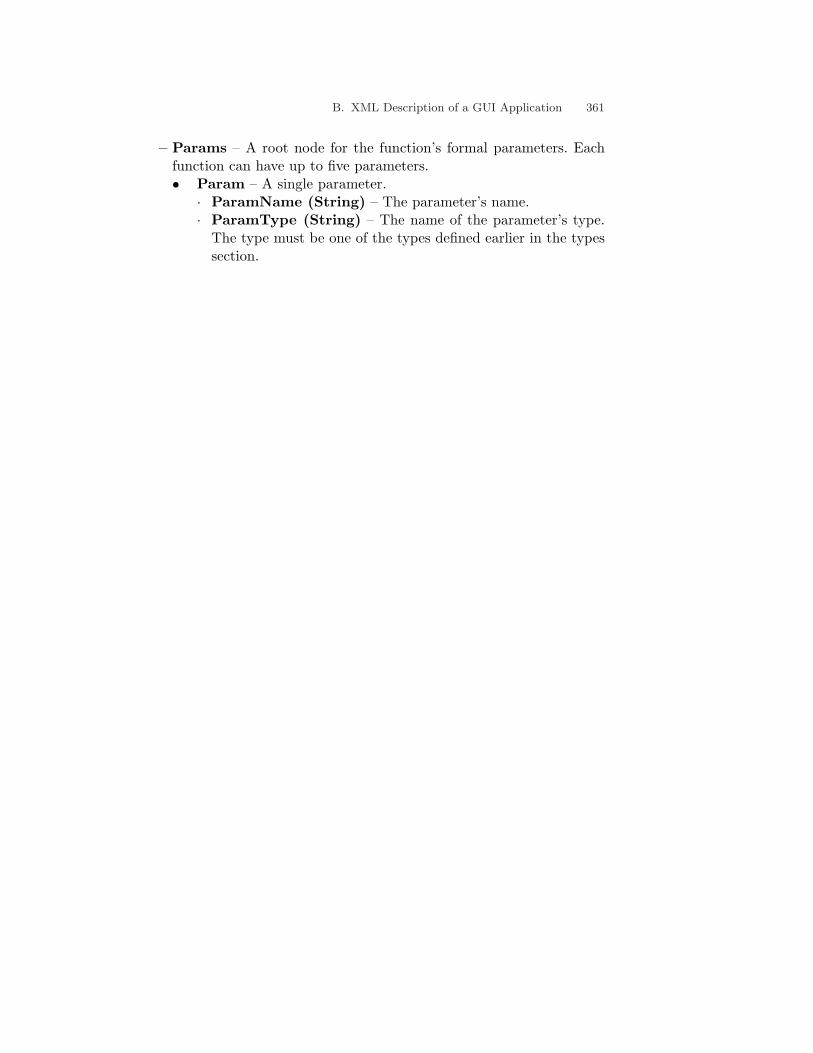
B. XML Description of a GUI Application 361
– Params – A root node for the function’s formal parameters. Eachfunction can have up to five parameters.• Param – A single parameter.
· ParamName (String) – The parameter’s name.· ParamType (String) – The name of the parameter’s type.
The type must be one of the types defined earlier in the typessection.


C. The Play-Engine Interface
This appendix describes IPlayEngine, an interface implemented by the Play-Engine and used by GUI applications to interact with it. The IPlayEngineinterface is installed as part of the Play-Engine installation, in the formof a COM (Component Object Model) component with the file name En-gineLib.dll.
The IPlayEngine interface has three methods:
ObjectClicked(ObjID: Integer) – The GUI application should call this methodwhenever a GUI object is clicked. The ObjID parameter should containthe ID of the clicked object.
ObjectChanged(ObjID: Integer, PropID: Integer, strValue: String) – The GUIapplication should call this method whenever a property of some objectis changed (e.g., clicking a switch to on, moving a slider, writing text ina text box, etc.). ObjID should contain the ID of the object, PropID theID of the modified property, and strValue the new value of the property.
ObjectRightClicked(ObjID: Integer) – The GUI application should call thismethod whenever a GUI object is right-clicked. The ObjID parametershould contain the ID of the right-clicked object.
C.1 Visual Basic Code
Here is the Visual Basic code for the IPlayEngine interface:Public Sub ObjectClicked(ByVal ObjID As Integer)End SubPublic Sub ObjectChanged(ByVal ObjID As Integer, PropID As Integer,strValue As String)End SubPublic Sub ObjectRightClicked(ByVal ObjID As Integer)End Sub

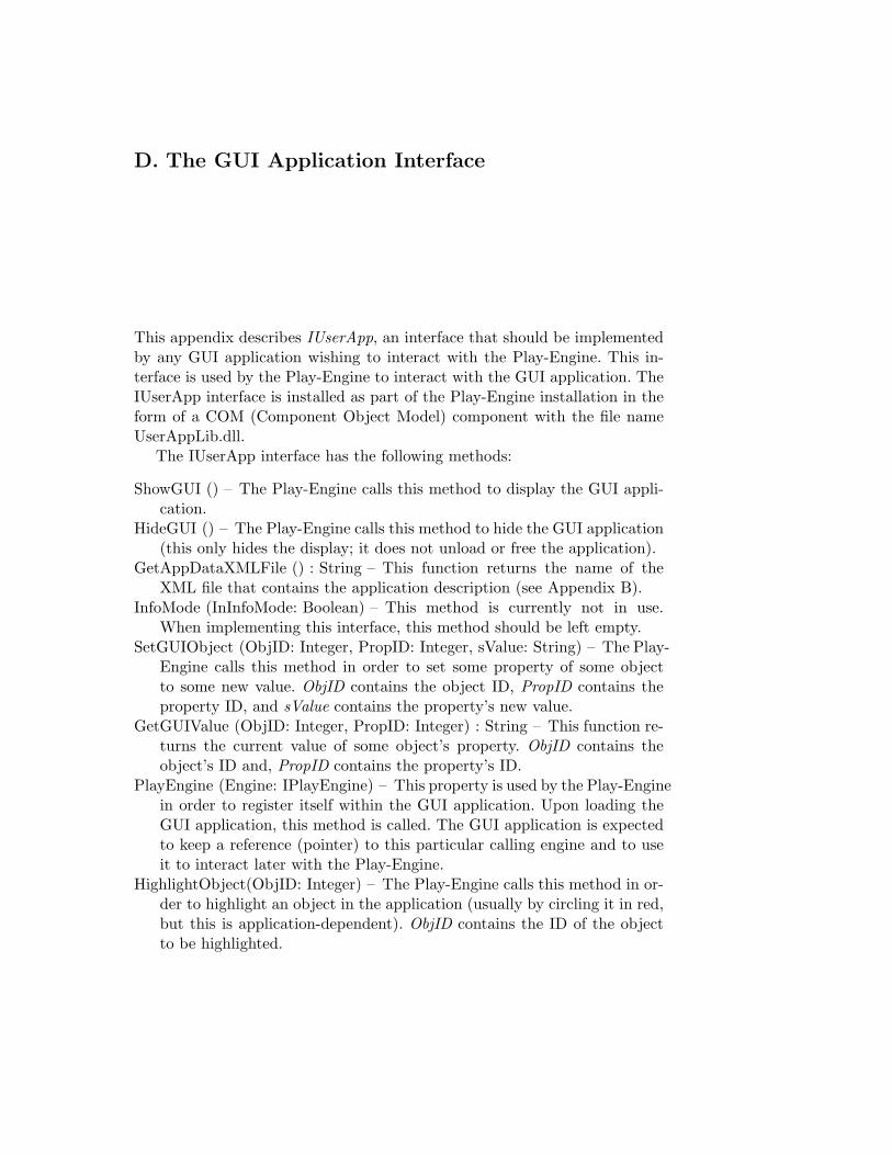
D. The GUI Application Interface
This appendix describes IUserApp, an interface that should be implementedby any GUI application wishing to interact with the Play-Engine. This in-terface is used by the Play-Engine to interact with the GUI application. TheIUserApp interface is installed as part of the Play-Engine installation in theform of a COM (Component Object Model) component with the file nameUserAppLib.dll.
The IUserApp interface has the following methods:
ShowGUI () – The Play-Engine calls this method to display the GUI appli-cation.
HideGUI () – The Play-Engine calls this method to hide the GUI application(this only hides the display; it does not unload or free the application).
GetAppDataXMLFile () : String – This function returns the name of theXML file that contains the application description (see Appendix B).
InfoMode (InInfoMode: Boolean) – This method is currently not in use.When implementing this interface, this method should be left empty.
SetGUIObject (ObjID: Integer, PropID: Integer, sValue: String) – The Play-Engine calls this method in order to set some property of some objectto some new value. ObjID contains the object ID, PropID contains theproperty ID, and sValue contains the property’s new value.
GetGUIValue (ObjID: Integer, PropID: Integer) : String – This function re-turns the current value of some object’s property. ObjID contains theobject’s ID and, PropID contains the property’s ID.
PlayEngine (Engine: IPlayEngine) – This property is used by the Play-Enginein order to register itself within the GUI application. Upon loading theGUI application, this method is called. The GUI application is expectedto keep a reference (pointer) to this particular calling engine and to useit to interact later with the Play-Engine.
HighlightObject(ObjID: Integer) – The Play-Engine calls this method in or-der to highlight an object in the application (usually by circling it in red,but this is application-dependent). ObjID contains the ID of the objectto be highlighted.

366 D. The GUI Application Interface
ClearObject(ObjID: Integer) – The Play-Engine calls this method in orderto remove the highlight from an object in the application. ObjID containsthe ID of the object to be de-highlighted.
GetObjectPosition(ObjID: Integer, Left: Integer reference, Top: Integer reference) –The Play-Engine calls this method in order to get the top and left coor-dinates of an object. ObjID contains the object’s ID. The returned valuesshould be placed in Left and Top, respectively.
GetObjectLayout(ObjID: Integer, Left: Integer reference, Top: Integer reference,Width: Integer reference, Height: Integer reference) – The Play-Enginecalls this method in order to get the layout information for an object.ObjID contains the object’s ID. The layout values should be placed inLeft, Top, Width and Height, respectively.
TerminateGUI () – The Play-Engine calls this method just before it termi-nates, thus giving the GUI application a chance to free memory andconduct all the actions needed for clean termination.
ApplyFunction(XMLFuncData: String) : String – This function is used bythe Play-Engine in order to compute the value of an implemented func-tion applied to given parameter values. XMLFuncData is a string thatcontains an XML description of the function to be applied. Its XMLstructure is as follows:• Function Info – The function information node
– Func Name (String) – The name of the implemented function.One of the functions that were declared in the implemented functionssection in the application XML description file.
– Param1 (String) – The value of parameter 1.– Param2 (String) – The value of parameter 2.– Param3 (String) – The value of parameter 3.– Param4 (String) – The value of parameter 4.– Param5 (String) – The value of parameter 5.If there are fewer than five1 parameters, only the relevant number ofparameters is given in the string.
D.1 Visual Basic Code
Here is the Visual Basic code for the IUserApp interface:Public Sub HideGUI()End Sub1 In the current implementation, there is a technical bound of up to five parameters. This
bound can be easily increased or avoided.

D.1 Visual Basic Code 367
Public Sub ShowGUI()End SubPublic Function ApplyFunction(XMLFuncData As String) As StringEnd FunctionPublic Property Get AppDataXMLFile() As StringEnd PropertyPublic Property Let InfoMode(InInfoMode As Boolean)End PropertyPublic Sub SetGUIObject(ObjID As Integer, PropID As Integer, sValue As
String)End SubPublic Function GetGUIValue(ObjID As Integer, PropID As Integer) As
StringEnd FunctionPublic Property Let PlayEngine(Engine As IplayEngine)End PropertyPublic Sub HighlightObject(ObjID As Integer)End SubPublic Sub ClearObject(ObjID As Integer)End SubPublic Sub GetObjectPosition(ObjID As Integer, ByRef Left As Integer,
ByRef Top As Integer)End SubPublic Sub GetObjectLayout(ObjID As Integer, ByRef Left As Integer,
ByRef Top As Integer, ByRef Width As Integer, ByRef HeightAs Integer)
End SubPublic Sub TerminateGUI()End Sub


E. The Structure of a (Recorded) Run
A recorded run of the Play-Engine is saved as an XML file, which can laterbe loaded and replayed. This appendix provides information on the structureof such an XML file and explains each of its fields. Knowing the structureof a run can be very useful if one wishes to create a run, either manuallyor by using another tool, and then load it into the Play-Engine. Runs cantherefore be generated by actual applications, by implementation tools, byconventional intra-object models, and so on.? Run – The root element of the Run XML file.
• ID (Integer) – The ID of the run.• Name (String) – The name of the run.• RunEvents – The root node for the events in the run.
– RunEvent – A single run event.• ID (Integer) – A unique ID for each event. Starts from 1 and is
continuously incremented.• Value (String) – If the event corresponds to a property change,
then the new property value is given here (for example, Off). If theevent corresponds to a method call between objects, the full string thatdescribes the method call is written here (for example, SetState(Off),Method1(X1,X2), and so on).
• EventKind (Send/Recv) – Indicates whether this is a send event ora receive event. For synchronous messages and for self-messages, onlythe Send event is specified in the run.
• FromObjID (Integer) – The ID of the object sending the message.This is the object ID that is specified in the application descriptionfile.
• ToObjID (Integer) – The ID of the object receiving the message.This is the object ID that is specified in the application descriptionfile. In the case of a self-message, ToObjID is the same as FromObjID.
• ToProperty (Integer) – The ID of the property that was changed.This is specified only if the parent run event describes a property valuechange, and is the ID associated with this property in the applicationdescription file.

370 E. The Structure of a (Recorded) Run
• Method (Integer) – The ID of the method that was called. Thisshould be specified only if the parent run event describes a method call,and is the ID associated with this method in the application descriptionfile.
• Param1 (String) – The value of parameter 1.• Param2 (String) – The value of parameter 2.• Param3 (String) – The value of parameter 3.• Param4 (String) – The value of parameter 4.• Param5 (String) – The value of parameter 5.
Parameter values are given only in the case of a method call. Whenthere are fewer than five parameters, only the relevant number of pa-rameters is given.

References
1. M. Abadi, L. Lamport, and P. Wolper. Realizable and Unrealizable Concurrent Pro-gram Specifications. In Proc. 16th Int. Colloq. Aut. Lang. Prog., vol. 372, LectureNotes in Computer Science, pp. 1–17. Springer-Verlag, 1989.
2. Altia Design & Altia FacePlate. Web page http://www.altia.com.3. R. Alur. Timed Automata. In 11th Int. Conf. on Computer-Aided Verification, vol.
1633, Lecture Notes in Computer Science, pp. 8–22. Springer-Verlag, 1999.4. R. Alur and D.L. Dill. A Theory of Timed Automata. Theoretical Computer Science,
126:183–235, 1994.5. R. Alur, K. Etessami, and M. Yannakakis. Inference of Message Sequence Charts.
In Proc. 22nd Int. Conf. on Software Engineering (ICSE’00), Limerick, Ireland, June2000.
6. R. Alur and T.A. Henzinger. Logics and Models of Real Time: a Survey. In Real-Time:Theory in Practice, REX Workshop, vol. 600, Lecture Notes in Computer Science, pp.74-106. Springer-Verlag, 1991.
7. R. Alur and T.A. Henzinger. A Really Temporal Logic. In Proc. 30th Annual Symp. onFoundations of Computer Science (FOCS’89), pp. 164–169. IEEE Computer SocietyPress, 1989.
8. R. Alur and T.A. Henzinger. Real-Time System = Discrete System + Clock Variables.Software Tools for Technology Transfer, 1:86–109, 1997.
9. R. Alur, G.J. Holzmann, and D. Peled. An Analyzer for Message Sequence Charts.Software Concepts and Tools, 17(2):70–77, 1996.
10. R. Alur and M. Yannakakis. Model Checking of Message Sequence Charts. In Proc.10th Int. Conf. on Concurrency Theory (CONCUR’99), Eindhoven, The Netherlands,August 1999.
11. D. Amyot and A. Eberlein. An Evaluation of Scenario Notations for Telecommunica-tion Systems Development. In Int. Conf. on Telecommunication Systems, Dallas, TX,2001.
12. K. Apt. Verification of Sequential and Concurrent Programs. Springer-Verlag, 2ndedition, 1997.
13. H. Ben-Abdallah and S. Leue. Timing Constraints in Message Sequence Chart Specifi-cations. In Proc. 10th Int. Conf. on Formal Description Techniques FORTE/PSTV’97,Osaka, Japan, November 1997. Chapman & Hall.
14. G. Berry and G. Gonthier. The Esterel Synchronous Programming Language: Design,Semantics, Implementation. Sci. Comput. Program., 19:87–152, 1992.
15. A.W. Biermann and R. Krishnaswamy. Constructing Programs from Example Com-putations. IEEE Trans. Softw. Eng., SE-2:141–153, 1976.
16. G. Booch. Object-Oriented Analysis and Design with Applications. Addison-Wesley,1994.
17. G. Booch, J. Rumbaugh, and I. Jacobson. Unified Modeling Language for Object-Oriented Development (Version 0.91 Addendum). RATIONAL Software Corporation,1996.
18. M. Broy and I. Kruger. Interaction Interfaces – Towards a Scientific Founda-tion of a Methodological Usage of Message Sequence Charts. In J. Staples, M.G.

372 References
Hinchey, Shaoying Liu Hinchey, and Shaoying Liu (ed.), Formal Engineering Methods(ICFEM’98), pp. 2–15. IEEE Computer Society, 1998.
19. F. Buschmann, R. Maunier, H. Rohnert, P. Sommerald, and M. Stal. A System ofPatterns. Pattern-Oriented Software Architecture. Wiley, 1996.
20. A.K. Chandra and P.M. Merlin. Optimal Implementation of Conjunctive Queries inRelational Databases. In Proc. 9th ACM Symp. on the Theory of Computing, pp.77–90, 1977.
21. P.P. Chen. The Entity-Relationship Model: Toward a Unified View of Data. ACMTrans. on Database Systems, 1:9–36, 1976.
22. E.M. Clarke, O. Grumberg, and D. Peled. Model Checking. MIT Press, 2000.23. A. Colmeraurer, H. Kanoui, P. Roussel, and R. Pasero. Un systeme de communication
homme-machine en francais. Technical Report, Group de Recherche en IntelligenceArtificielle, Univ. d’Aix-Marseille, 1973.
24. Microsoft COM. Web page: http://www.microsoft.com/com.25. L. Constantine and E. Yourdon. Structured Design. Prentice-Hall, 1979.26. S. Cook and J. Daniels. Designing Object Systems: Object-Oriented Modeling with
Syntropy. Prentice-Hall, 1994.27. W. Damm and D. Harel. LSCs: Breathing Life into Message Sequence Charts. Formal
Methods in System Design, 19(1), 2001. Preliminary version in Proc. 3rd IFIP Int.Conf. on Formal Methods for Open Object-Based Distributed Systems (FMOODS’99),pp. 293–312, P. Ciancarini, A. Fantechi and R. Gorrieri, (eds.), Kluwer, 1999.
28. W. Damm, B. Josko, and R. Schlor. Specification and Verification of VHDL-BasedSystem-Level Hardware Designs. In E. Borger (ed), Specification and Validation Meth-ods, pp. 331–410. Oxford University Press, 1995.
29. W. Damm and J. Klose. Verification of a Radio-Based Signalling System Usingthe STATEMATE Verification Environment. Formal Methods in System Design,19(2):121–141, 2001.
30. Borland Delphi. Web page http://www.borland.com/delphi/.31. T. DeMarco. Structured Analysis and System Specification. Yourdon Press, 1978.32. L.K. Dillon, G.Kutty, L.E. Moser, P.M. Melliar-Smith, and Y.S. Ramakrishna. A
Graphical Interval Logic for Specifying Concurrent Systems. ACM Trans. on Soft.Eng. and Meth., Vol 3(2), pp. 131–165, 1994.
33. R.G. Dromey. Genetic Software Engineering. Manuscript, 2001.34. E.A. Emerson and E.M. Clarke. Using Branching Time Temporal Logic to Synthesize
Synchronization Skeletons. Science of Computer Programming, 2:241–266, 1982.35. e-SIM Rapid. Web page http://www.e-sim.com/home/.36. Macromedia Flash. Web page http://www.macromedia.com/software/flash/.37. R.W. Floyd. Assigning Meanings to Programs. In Proc. Symp. on Applied Math., vol.
19: Mathematical Aspects of Computer Science, pp. 19–32. American MathematicalSociety, 1967.
38. I. Greenwald. Development of the vulva. In: D.L. Riddle, , T. Blumenthal, B.J. Meyer,and J.R. Priess (eds.) C. elegans vol. II pp. 519–541. Cold Spring Harbor LaboratoryPress, 1997.
39. R. Grosu, I. Kruger, and T. Stauner. Hybrid Sequence Charts. Tech. Report TUM-I9914, Technical University of Munich, 1999.
40. E.L. Gunter, A. Muscholl, and D. Peled. Compositional Message Sequence Charts. InTools and Algorithms for Construction and Analysis of Systems, vol. 2031 of LectureNotes in Computer Science pp. 496–511. Springer-Verlag, 2001.
41. N. Halbwachs, P. Caspi, P. Raymond, and D. Pilaud. The Synchronous Data-FlowProgramming Language LUSTRE. Proc. IEEE, 79(9):1305–1320, September 1991.
42. D. Harel. Statecharts: A Visual Formalism for Complex Systems. Sci. Comput. Prog.,pp. 231–274, 1987. (Preliminary version: Tech. Report CS84-05, The Weizmann Insti-tute of Science, Rehovot, Israel, February 1984.)
43. D. Harel. From Play-In Scenarios to Code: An Achievable Dream. IEEE Computer,pp. 53–60, January 2001.

References 373
44. D. Harel and E. Gery. Executable Object Modeling with Statecharts. IEEE Computer,pp. 31–42, 1997.
45. D. Harel and Y. Koren. Drawing Graphs with Non-uniform Vertices. In Proc. WorkingConf. on Advanced Visual Interfaces (AVI’02), pp. 157–166. ACM Press, 2002.
46. D. Harel and H. Kugler. Synthesizing State-Based Object Systems from LSC Specifica-tions. Int. J. of Foundations of Computer Science (IJFCS), 13(1):5–51, Febuary 2002.(Also, Proc. 5th Int. Conf. on Implementation and Application of Automata (CIAA2000), July 2000, vol. 2088, Lecture Notes in Computer Science. Springer-Verlag, 2000.)
47. D. Harel, H. Kugler, R. Marelly, and A. Pnueli. Smart Play-Out of Behavioral Re-quirements. In Proc. 4th Int. Conf. on Formal Methods in Computer-Aided Design(FMCAD’02), Portland, USA, 2002. Also available as Tech. Report MCS02-08, TheWeizmann Institute of Science, 2002.
48. D. Harel, H. Lachover, A. Naamad, A. Pnueli, M. Politi, R. Sherman, A. Shtull-Trauring, and M. Trakhtenbrot. STATEMATE: A Working Environment for theDevelopment of Complex Reactive Systems. IEEE Trans. Soft. Eng., 16:403–414,1990. (Preliminary version in Proc. 10th Int. Conf. Soft. Eng. pp. 396–406. IEEEPress, 1988).
49. D. Harel and R. Marelly. Specifying and Executing Behavioral Requirements: ThePlay-In/Play-Out Approach. Software and System Modeling (SoSyM), to appear,2003.
50. D. Harel and R. Marelly. Play-Engine User’s Guide. 3rd edition, 2002.51. D. Harel and R. Marelly. Playing with Time: On the Specification and Execution of
Time-Enriched LSCs. In Proc. 10th IEEE/ACM Int. Symp. on Modeling, Analysisand Simulation of Computer and Telecommunication Systems (MASCOTS’02), FortWorth, Texas, 2002.
52. D. Harel and A. Pnueli. On the Development of Reactive Systems. In K. R. Apt, (ed.),Logics and Models of Concurrent Systems, NATO ASI Series, Vol. F-13, pp. 477–498.Springer-Verlag, 1985. 1985.
53. D. Harel and M. Politi. Modeling Reactive Systems with Statecharts: The STATEM-ATE Approach. McGraw-Hill, 1998. Early version titled The Languages of STATE-MATE, Technical Report, I-Logix, Inc., Andover, MA (250 pp.), 1991.
54. D. Hatley and I. Pirbhai. Strategies for Real-Time System Specification. Dorset House,1987.
55. C. Heitmeyer, J. Kirby, B. Labaw, and R. Bharadwaj. SCR*: A Toolset for Specifyingand Analyzing Software Requirements. In A.J. Hu and M.Y. Vardi (eds.), Int. Conf.on Computer Aided Verification (CAV’98), vol. 1427 of Lecture Notes in ComputerScience, pp. 5–51. Springer-Verlag, 1998.
56. J.G. Henriksen, M. Mukund, K. Narayan Kumar, and P.S. Thiagarajan. On MessageSequence Graphs and Finitely Generated Regular MSC Languages. In Proc. 27th Int.Colloq. on Automata Languages and Programming (ICALP’2000), Geneva, Switzer-land, 2000, vol. 1853 of Lecture Notes in Computer Science. Springer-Verlag.
57. J.G. Henriksen, M. Mukund, K. Narayan Kumar, and P.S. Thiagarajan. RegularCollections of Message Sequence Charts. In Proc. of the 25th Int. Symp. on Mathe-matical Foundations of Computer Science (MFCS’2000), vol. 1893 of Lecture Notes inComputer Science, Bratislava, Slovakia, 2000. Springer-Verlag.
58. C.A.R. Hoare. An Axiomatic Basis for Computer Programming. Comm. Assoc. Com-put. Mach., 12(10):576–583, 1969.
59. C.A.R. Hoare. Communicating Sequential Processes. Comm. Assoc. Comput. Mach.,21:666–677, 1978.
60. I-Logix, Inc. Products Web page. http://www.ilogix.com/fs prod.htm.61. American National Standards Institute. Reference Manual for the ADA Programming
Language. February 1983. ANSI/MIL-STD 1815A. Also published by Springer-Verlagas vol. 155 of Lecture Notes in Computer Science.
62. I. Jacobson. Object-Oriented Software Engineering: A Use Case Driven Approach.Addison-Wesley, 1992.

374 References
63. N. Kam, D. Harel, H. Kugler, R. Marelly, A. Pnueli, E.J.A. Hubbard, and M.J. Stern.Formal Modeling of C. elegans Development: A Scenario-Based Approach. In Proc.Int. Workshop on Computational Methods in Systems Biology (CMSB 2003). Kluwer,February 2003.
64. J. Klose and B. Westphal. Relating LSC Specifications to UML Models. In Proc. 2ndInt. Workshop on Integration of Specification Techniques for Applications in Engineer-ing (INT 2002), Grenoble, France, 2002.
65. J. Klose and H. Wittke. An Automata Based Interpretation of Live Sequence Charts.In Proc. 7th Intl. Conf. on Tools and Algorithms for the Construction and Analysis ofSystems (TACAS’01), 2001.
66. K. Koskimies and E. Makinen. Automatic Synthesis of State Machines from TraceDiagrams. Software — Practice and Experience, 24(7):643–658, 1994.
67. K. Koskimies, T. Mannisto, T. Systa, and J. Tuomi. SCED: A Tool for DynamicModeling of Object Systems. Tech. Report A-1996-4, University of Tampere, July1996.
68. K. Koskimies, T. Systa, J. Tuomi, and T. Mannisto. Automated Support for ModelingOO Software. IEEE Software, 15(1):87–94, 1988.
69. R.A. Kowalski. Predicate Logic as a Programming Language. Information Process-ing’74, pp. 569–574. North-Holland, 1974.
70. R. Koymans, J. Vytopil, and W.-P. de Roever. Real-Time Programming and Asyn-chronous Message Passing. In Proc. 2nd Annual Symp. on Principles of DistributedComputing, pp. 187–197. ACM Press, 1983.
71. I. Krueger. Distributed System Design with Message Sequence Charts. Ph.D. Thesis,Department of Informatics, Technical University of Munich, 2000.
72. I. Kruger, R. Grosu, P. Scholz, and M. Broy. From MSCs to Statecharts. In Proc.DIPES’98. Kluwer, 1999.
73. O. Kupferman and M.Y. Vardi. Synthesis with Incomplete Information. In 2nd Int.Conf. on Temporal Logic, pp. 91–106, Manchester, July 1997.
74. L. Lamport. Time, Clocks, and the Ordering of Events in a Distributed System.Communications of the ACM, Vol 21(7), pp. 558–565, 1978.
75. L. Lamport. The Temporal Logic of Actions. ACM Trans. on Prog. Lang. and Sys.,Vol 16(3), pp. 872–923, 1994.
76. M. Lettrari and J. Klose. Scenario-Based Monitoring and Testing of Real-Time UMLModels. In 4th Int. Conf. on the Unified Modeling Language, Toronto, October 2001.
77. S. Leue, L. Mehrmann, and M. Rezai. Synthesizing ROOM Models from MessageSequence Chart Specifications. Tech. Report 98-06, University of Waterloo, April1998.
78. M. Broy, C. Hofmann, I. Kruger, and M. Schmidt. A Graphical Description Techniquefor Communication in Software Architectures. Tech. Report TUM-I9705, TechnicalUniversity of Munich, 1997.
79. P.W. Sternberg and M. Wang. Pattern Formation During C. elegans Vulval Induction.Curr. Top. Dev. Biol., 51:189–220, 2001.
80. J. Magee and J. Kramer. Concurrency - State Models & Java Programs. Wiley, 1999.81. J. Magee, N. Pryce, D. Giannakopoulou, and J. Kramer. Graphical Animation of
Behavior Models. 22nd Int. Conf. on Soft. Eng. (ICSE’00), Limeric, Ireland, 2000.82. Z. Manna and A. Pnueli. The Temporal Logic of Reactive and Concurrent Systems:
Specification. Springer-Verlag, 1992.83. Z. Manna and R.J. Waldinger. A Deductive Approach to Program Synthesis. ACM
Trans. on Programming Languages and Systems, 2:90–121, 1980.84. R. Marelly, D. Harel, and H. Kugler. Multiple Instances and Symbolic Variables in
Executable Sequence Charts. In Proc. 17th Ann. ACM Conf. on Object-Oriented Pro-gramming, Systems, Languages and Applications (OOPSLA’02), Seattle, WA, 2002.
85. S. Mauw and M.A. Reniers. Refinement in Interworkings. In U. Montanari andV. Sassone (eds.), CONCUR’96, vol. 1119 of Lecture Notes in Computer Science, pp.671–686. Springer, 1996.
References 375
86. N. Meng-Siew. Reasoning with Timing Constraints in Message Sequence Charts. Mas-ter’s Thesis, University of Stirling, UK, August 1993.
87. B. Meyer. Eiffel: The Language. Prentice-Hall, 1992.88. R. Milner. A Calculus of Communicating Systems, vol. 92 of Lecture Notes in Com-
puter Science. Springer-Verlag, 1980.89. B. Moszkowski. A Temporal Logic for Multi-level Reasoning about Hardware. IEEE
Computer, 18:10–19, 1985.90. B. Moszkowski. Executing Temporal Logic Programs. Cambridge University Press,
Cambridge, UK, 1986.91. ITU-TS Recommendation Z.120 (11/99): MSC 2000. ITU-TS, Geneva, 1999.92. A. Pnueli. The Temporal Semantics of Concurrent Programs. Theoretical Computer
Science, 13:1–20, 1981.93. A. Pnueli. Applications of Temporal Logic to the Specification and Verification of
Reactive Systems: A Survey of Current Trends. In de Bakker et al. (eds.), CurrentTrends in Concurrency , vol. 224 of Lecture Notes in Computer Science, pp. 510–584.Springer-Verlag, 1986.
94. A. Pnueli and W.-P. de Roever. Rendez-vous with Ada: A Proof Theoretical View. InProc. SIGPLAN AdaTEC Conf. on Ada, pp. 129–137. ACM Press, 1982.
95. A. Pnueli and E. Harel. Applications of Temporal Logic to the Specification of Real-Time Systems. In M. Joseph (ed.), Formal Techniques in Real-Time and Fault-TolerantSystems, vol. 331 of Lecture Notes in Computer Science, pp. 84–98. Springer-Verlag,1988.
96. A. Pnueli and R. Rosner. On the Synthesis of an Asynchronous Reactive Module.In Proc. 16th Int. Colloq. Aut. Lang. Prog., vol. 372 of Lecture Notes in ComputerScience, pp. 652–671. Springer-Verlag, 1989.
97. A. Pnueli and R. Rosner. Distributed Reactive Systems Are Hard To Synthesize. InProc. 31th IEEE Symp. Found. of Comp. Sci., pp. 746–757, 1990.
98. A. Pnueli and R. Rosner. On the Synthesis of a Reactive Module. In Proc. 16th ACMSymp. on Principles of Programming Languages, pp. 179–190, Austin, TX, January1989.
99. N. Pryce and J. Magee. SceneBeans: A Component-Based Animation Framework forJava. http://www-dse.doc.ic.ac.uk/Software/SceneBeans/.
100. Rational, Inc. Web page http://www.rational.com.101. W. Reisig. Petri Nets: An Introduction. Springer-Verlag, 1985.102. M.A. Reniers. Message Sequence Charts. Syntax and Semantics. Ph.D. Thesis, Eind-
hoven University of Technology, 1999.103. J.A. Robinson. Logic: Form and Function, Chap. 11, pp. 182–198. North-Holland,
1979.104. A. Roychoudhury and P.S. Thiagarajan. Interface Modeling with Cyclic Transaction
Processes. In Formal Methods at the Crossroads: From Panacea to Foundation Sup-port, 10th Anniversary Colloq. of UNU/IIST, Lisbon, Portugal, 2002, Lecture Notesin Computer Science, Springer-Verlag, to appear.
105. J. Rumbaugh, M. Blaha, W. Premerlani, F. Eddy, and W. Lorensen. Object-OrientedModeling and Design. Prentice-Hall, 1991.
106. J. Rumbaugh, I. Jacobson, and G. Booch. The Unified Modeling Language ReferenceManual. Addison-Wesley, 1999.
107. S. Bornot and J. Sifakis. An Algebraic Framework for Urgency. Information andComputation, 163:172–202, 2000.
108. R. Schlor and W. Damm. Specification and Verification of System-Level HardwareDesigns using Timing Diagram. In Proc. European Conf. on Design Automation, Paris,France, 1993, pp. 518–524. IEEE Computer Society Press.
109. R. Schlor, B. Josko, and D. Werth. Using a Visual Formalism for Design Verifica-tion in Industrial Environments. In T. Margaria, B. Steffenan, R. Ruckert, and J.Posegga (eds.), Services and Visualization: Towards User-Friendly Design, ACoS’98,

376 References
VISUAL’98, AIN’97, Selected Papers, vol. 1385 of Lecture Notes in Computer Science,pp. 208–221. Springer-Verlag, 1998.
110. SDL: ITU-T Recommendation Z.100, Languages for Telecommunications Applica-tions: Specification and Description Language, Geneva, 1999.
111. B. Selic, G. Gullekson, and P. Ward. Real-Time Object-Oriented Modeling. Wiley,1994.
112. J. Sifakis. Modeling Real-Time Systems – Challenges and Work Directions. In EM-SOFT01, Tahoe City, CA, USA, October 2001, vol. 2211 of Lecture Notes in ComputerScience, Springer-Verlag.
113. J. Suzuki and Y. Yamamoto. Extending UML for Modelling Reflective SoftwareComponents. In R. France and B. Rumpe (eds.), UML’99 — the Unified ModelingLanguage. Beyond the Standard. 2nd Int. Conf., Fort Collins, CO, USA, 1999, vol.1723 of Lecture Notes in Computer Science, pp. 220–235. Springer-Verlag, 1999.
114. S. Uchitel, J. Kramer, and J. Magee. Detecting Implied Scenarios in Message SequenceChart Specifications. In 9th European Software Engineering Conferece and 9th ACMSIGSOFT Int. Symp. on the Foundations of Software Engineering (ESEC/FSE’01).Vienna, Austria., September 2001.
115. Documentation of the Unified Modeling Language (UML), available from the ObjectManagement Group (OMG). http://www.omg.org.
116. Microsoft Visual Basic. Web page http://msdn.microsoft.com/vbasic/.117. P. Ward and S. Mellor. Structured Development for Real-Time Systems, vol. 1–3.
Yourdon Press, 1985.118. D.H.D. Warren. Implementing Prolog – Compiling Logic Programs (1 and 2). DAI
Research Reports 39 and 40, University of Edinburgh, 1977.119. J. Whittle and J. Schumann. Generating Statechart Designs from Scenarios. In 22nd
Int. Conf. on Software Engineering (ICSE 2000), pp. 314–323. ACM Press, 2000.120. R.J. Wieringa. Design Methods for Reactive Systems: Yourdon, Statemate, and the
UML. Morgan Kaufmann, 2002.121. H. Wong-Toi and D.L. Dill. Synthesizing Processes and Schedulers from Temporal
Specifications. In Computer-Aided Verification ’90, DIMACS Series in Discrete Math-ematics and Theoretical Computer Science, vol. 3, pp. 177–186, 1991.
122. Web page http://www.xml.com.123. ITU-TS Recommendation Z.120: Message Sequence Chart (MSC). ITU-TS, Geneva,
1996.124. ITU-TS Recommendation Z.120: Message Sequence Chart (MSC) — Annex B: Alge-
braic Semantics of Message Sequence Charts. ITU-TS, Geneva, 1995.

Index
activation modes– active, 67– check, 161– completed, 161– preactive, 67– terminate, 161Ada, 249Altia FacePlate, 322anti-scenario, 5, 15, 17, 59, 125, 251– automatic creation, 304application type, see typeassignment, 35, 108–111, 231, 295– affecting a variable, 111– assigned-to variable, 35, 108– definition, 115, 243– in precharts, 113– monitoring, 161– semantics of, 339– storing constants, 111– storing functions, 111– storing properties, see property, store– synchronize, 111– using a variable, 111
basic expression, see condition, basicexpression
behavior, 14– debugging, 19– inter-object, VII, 4, 14, 65, 211, 282– intra-object, 4, 14, 211– refinement and composition, 326behavior tree, see GSEbelongs relation, 221– semantics of, 339Bind procedure, 102– semantics of, 348binding expression, see instance, symbolicbiology, 302– surprising biologists, 304Booch method, 12Borland Delphi, 322bounded temporal operator, 230breakpoint, 315
C. elegans, 301– development, 307– GUI, 301CCITT, 13, 59CCS, 10class, 38, 209, 300– adding, 211– definition, 58, 201– in a scenario, 210–212– inheritance, 212, 327– instance, 210– organization, 327– semantics of, 335– vs. interface, 328clock, 46, 231– automatic mode, 46, 238– instance, 46, 231, 235– interval, 238– manual mode, 46, 238– object, 236– – definition, 242– – semantics of, 336– Tick button, 46, 236– Tick method, 231– Time property, 231clock variable, 230, 231, 248closed system, 205code, 211code generation, 11COM, 317, 322component object model, see COMcondition, 119–128, 231, 286, 293– arranging tool tips, 123– basic expression, 121– – dialog, 122, 123– – semantics of, 340– cold, 31, 119, 295– conjunctive query, 121– constraining a variable, 124– constraining properties, 122– definition, 128– dialog, 30, 122– displaying, 123

378 Index
– execution policies, 126– forbidden, see forbidden condition– free expression, 30, 125– hot, 31, 120, 294– – in anti-scenarios, 125– in if-then-else, 134– in loops, 34, 176, 251– in precharts, 127– monitoring, 161– participating instances, 32, 120– probabilities, 125, 300– relation operators, 30– reserved words, 124– SELECT, 125– semantics of, 339– stand-alone, 31– SYNC, 34– synchronize, 31, 121, 123– tooltip, 41– TRUE, 34– using a variable, 126– wizard, 31Connect procedure, 101, 348constructs– assignment, see assignment– if-then-else, see if-then-else– loop, see loop– subchart, see subchartcontrol signal, see methodCSP, 10CTL, 206CTL∗, 206cursor, 26cut, 67, 264– AdvanceCut function, 345– BeginMainCut function, 345– cold, 153– definition, 77– InitialCut function, 345– semantics of, 344– temperature, 67, 78– – semantics of, 345
delay, 230, 249delay interval, 230, 247delayed deadline, 249design, 189–201, 325– activities, 189– by teams, 198– debugging, 45, 197– patterns, 190– traceability, 195– transition from requirements, 44, 189– working with interfaces, 199discrete system, 231
drawing rule, 231, 247
e-SIM Rapid, 322EET, 81Eiffel, 278entity-relationship diagrams, 10environment, 36, 64, 198–200, 264, 286, 299– interaction with, 38– play-out, 42Esterel, 10, 249event– cold-forbidden, 276– – semantics of, 350– definition, 75– enabled, 67, 130, 289– – definition, 78– – semantics of, 346– hidden, 76, 112, 126– hot-forbidden, 275– – semantics of, 350– injecting, 164, 165– LSC event vs. system event, 342– minimal, 67, 113, 116, 161– – definition, 78– – semantics of, 345– reachable, 143, 184– – semantics of, 346– receive, 59– semantics of, 341– send, 59– violating, 67, 266, 271– – definition, 78– – semantics of, 346– visible, 76, 157examples– bakery, 25– C. elegans, 301– cellular phone, 91– cruise control system, 251– pocket calculator, 105– telephone network, 209external change, see environment, play-outexternal environment, see environmentexternal event manager, 164– event queue, 165external objects, see object, external
first-order logic, 248forbidden condition, 258–261– cold, 259– definition, 269– hot, 259– semantics of, 341forbidden element, 251–266, 300– active scope, 270– – semantics of, 350

Index 379
– contained scopes, 263– dominant, 262– dominant function, 271– – semantics of, 351– scope, 253, 262–263– – semantics of, 341– time constraints, 266forbidden message, 252–258– adding, 255– cold, 253– definition, 269– exact, 255– hot, 253– levels of generality, 255–256– semantics of, 341– symbolic, 255– symbolic instances, 256– temperature, 253freeze quantifier, 230, 248function information structure, 114– semantics of, 337function library, 320functional decomposition, 9future work, 190, 214, 325–331
genetic software engineering, see GSEgraph layout, 132GSE, 206guards, see condition, stand-aloneGUI application, VII, 22, 84, 189, 309, 317– XML description, 359GUI controls, see GUIEdit, custom controlsGUI Editor, see GUIEditGUIEdit, 83, 317–322– add-on, 318– as proof of concept, 322– building the GUI, 319– custom controls, 321– defining objects, 319– defining types, 319– generating application file, 320– generating code, 320– hook procedures, 320– loading functions, 320– modifying applications, 321– toolbar, 318
hierarchical MSCs, see HMSCsHMI, 322HMSCs, 146, 188HySC, 81
I-Logix, 10IDE, 322if-then-else, 30, 133–134, 297
– definition, 142– in precharts, 138– monitoring, 139, 161– nested, 157– scheduling policies, 140– semantics of, 341– wizard, 137implemented function, 36, 105–108, 299,
320– actual parameters, 106– binary, 107– definition, 114– formal parameters, 105– semantics of, 336– XML description, 360inductive assertions, 12, 20information passing, see methodinitial configuration, see jump startinstance, 26, 59– clock, see clock, instance– definition, 75, 221– locations, see location– semantics of, 338– symbolic, 38, 209–220, 300– – binding, 42, 210, 213, 327– – binding expression, 213–215, 217, 327– – existential, 215– – in existential charts, 218– – in forbidden messages, 256– – playing in, 212– – quantification, 215–216– – scenario prefix, 216– – static binding, 213– – symmetric precharts, 227– – universal, 215– – wizard, 214interface, 328internal object, see object, internalinterval temporal logic, 82, 278interworkings, 81invariant, 13, 251, 278– class level, 278IPlayEngine, 86, 363ITL, see interval temporal logicITU, 13, 59IUserApp, 86, 317, 320, 365
J2SE, 322Java, 322Java foundation class, see JFCJFC, 322jump start, 314
live copy, 67, 155, 161, 216, 289, 299– definition, 79, 167– life cycle, 67, 161

380 Index
– semantics of, 345live sequence charts, see LSCliveness constraints, 13location, 59, 61, 292– affecting a variable, 96– cold, 61– conflicts with messages, 71–73– final, 59– hot, 61– initial, 59loop, 33, 175–183, 297– adding elements, 176– bounded, see loop, fixed– definition, 183– dynamic, 178, 182, 299– – monitoring, 181– end, 176– exiting, 183– fixed, 34, 176, 298– in MSCs, 187– infinite, see smart play-out, detecting
infinite loops– monitoring vs. executing, 181– number of iterations, 178– playing in, 176– prompting for iterations, 182– repeat until, 177– run-time information, 41– runtime information, 178– semantics of, 341– unbounded, 176, 240, 266, 298– while do, 177– wizard, 33, 176LSC, VII, 6, 16, 22, 26, 59–81, 251, 325– activation, 67, 290, 293– activation condition, 82– as final implementation, 23– automata-based semantics, 248– background color, 314– breakpoint, see breakpoint– chart body, see main chart– clone, see live copy– completion, 41, 69, 161– consistency, 206– constant, 60– copy, see live copy– cut, see cut– definition, 75– executing vs. monitoring, 165–166– existential, 43, 60, 159, 161, 162, 196,
286, 312– – satisfying, see smart play-out, satisfying
existential charts– forbidden element, see forbidden element– forbidden elements area, 255
– forbidden elements header, 254– main chart, 293– monitoring, 160–163, 165, 171– natural language description, 62– playing in, 62–65– playing out, 65–71– prechart, see prechart– recursion, 155– refinement, 190– semantics of, 338– simultaneous activation, 155– specification, 75– statistics, see Play-Engine, statistics– strict, 267– time extensions, see time– tolerant, 267– tolerant semantics, 266–268– universal, 22, 39, 60, 287, 293, 312– violation, 161, 254, 255, 259, 264– watchdog, 266LSC event– semantics of, see event, semantics ofLSC message– semantics of, 339LSC specification– semantics of, 338–344Lustre, 10
Macromedia Flash, 322main chart, see LSC, main chartmessage, 26, 59, 291– asynchronous, 61, 290– cold, 61– conflicts with locations, see location,
conflicts with messages– definition, 74, 99, 201– exact, 93– forbidden, see forbidden message– hot, 61– self, 27, 61– semantics of, see system message,
semantics of; LSC message, semantics of– symbolic, 27, 91–99, 133, 209, 296– synchronous, 61– – semantics of, 337message content– semantics of, 337message delivery interval, 247message sequence charts, see MSCsmethod, 193–196– asynchronous, 193– definition, 201– in object map, 193– semantics of, 336– synchronous, 193

Index 381
method information structure, 201– semantics of, 337Microsoft Visual Basic, 318, 322model– intra-object, 164model checking, 20, 248, 307model execution, 10monitor-event, 165, 166, 170, 187, 275, 356MSCs, 13, 59, 81, 187, 247– high-level, see HMSCs– MSC 2000, 81multiple charts, see play-out, multiple
charts
navigation expression, 327nondeterministic choice, see condition,
probabilities, 135–136note, 314
object, 319– abstract, 326– associate with class, 211– composition, 325– definition, 58, 201– dialog, 191, 193– dynamic creation and destruction, 209,
328–329– external, 198–201– – controlling behavior, 199– – interacting with, 199– hierarchy, 325– internal, 190–193, 325– – adding, 191, 211– – playing in, 193– methods, see method– properties, see property– refinement, 190, 325– semantics of, 335– sub-object, 326– XML description, 359object interaction, see methodobject map, 45, 192, 251, 309object model, 213object model diagram, 10, 12, 192, 227, 327object oriented, 10, 209– analysis and design, 10object system, 55– semantics of, 335ObjectTime, 11OCL, 132OMG, 12OMSC, 81OMT, 12OOAD, see object oriented, analysis and
design
open system, 205operational semantics, 344–358– transition system, see transition systemoverlapping charts, see play-out, overlap-
ping charts
parameterized instance, see instance,symbolic
parameterized system, 209partial order, 15, 59, 254– definition, 76– enriching with variables, 94– semantics of, 342–344Petri nets, 10Play-Engine, VII, 21, 26, 83–86, 152, 164,
238, 282, 301, 318, 325– additional features, 313–315– application description file, 320, 359–361– application extension, 86– application interface, 309, 311– application section, 84– architecture, 309–313– – play-in, 310– – play-out, 311– breakpoint, see breakpoint– connecting, 330– connecting two engines, 165, 313– Execution manager, 312, 313– External manager, 313– GUI manager, 310, 312– interfaces, 86– look and feel, 83– LSC monitor, 312– notes, see note– ObjectMap manager, 310, 312– Play-Engine interface, 309, 310– run file, 313– Run manager, 313– run-time information, 314– saving files, 85– Sequence manager, 311– specification section, 85– statistics, 315– user guide, 323– workspace file, 86play-in, VII, 6, 21, 26, 310, 325– conditions, 121– if-then-else, 137– subcharts, 136play-in scenarios, 21play-in/play-out approach, 21– overview, 25play-out, VII, 6, 22, 39, 282, 311, 325– animating interactions, 45, 197– assignments, 111

382 Index
– conditions, 126– forbidden elements, 264– general schema, 66, 153, 160– if-then-else, 138– internal objects, 196– loops, 178– maximal approach, 153– minimal approach, 153– monitoring, 43, 312– monitoring dynamic loops, 181– multiple charts, 149–153– overlapping charts, 154–157, 161– participating LSCs, 315– smart, see smart play-out– symbolic messages, 99– time, 237–239– tracing, see play-out, monitoringpost-condition, 13, 278pre-condition, 13, 278prechart, 26, 60, 290, 292– violation, 70, 151, 218, 292primitive recursive functions, 178processor speed interval, 247property, 56–57, 294, 319– adding, 190– affects, 57, 61, 64– changed externally, 57– default, 57– definition, 58– in object map, 192– in only, 57– prefix, 56, 92– semantics of, 336– store, 35, 108– structured, 329– synchronous, 57– XML description, 360prototype, 22
quantified object binding, 215
Rational, 11reachable event, see event, reachablereactive system, VII, 3, 10, 36, 198, 281– programming, 6reactivity, 3real-time system, 10, 46, 231, 248recursive functions, 178regression tests, see testing, regressionrequirements, 6, 12, 165, 196, 198, 281– component-based, 201– executing, 65– liveness, 13– safety, 13– violation, 254, 259
reserved words, see condition, reservedwords
Rhapsody, 11, 19, 171ROOM, 11, 205Rose RealTime, 11run– consistent, 67, 161, 169– – definition, 80– – semantics of, 355– definition, 80– importing, 44, 164– manipulations, 164– recorded, 162, 369– recorded event, 164– recording and replaying, 44, 162–164,
196, 304– semantics of, 355– trace, 162
safety constraints, 13SCED, 205scenario, VII, 3, 13, 189– anti, see anti-scenario– fragment, 48, 134, 151– generic, 15, 209, 296, 327– multiple, see multiple charts– provisional, 161– satisfying, 161– symbolic, 91scenario fragment, 282SCR, 206SDL, 10SDT, see timing diagramsSEC, 330SELECT, see condition, SELECT, 135– in a loop, 177sequence diagram, 13, 14, 59, 81, 171smart play-out, 47, 281–306– as verification problem, 287– assignments, 295– complexity, 288– conditions, 293– detecting infinite loops, 285– examples, 283–287– if-then-else, 297– limitations, 299– loops, 297– LSC activation, 293– messages, 291– model checking, 50, 281, 290– – formula, 298– nondeterminism, 48, 282– prechart, 292– satisfying existential charts, 286, 301–306– semantics, 300

Index 383
– symbolic messages, 296– transition system, 290– variables, 296software cost reduction, see SCRsquiggle, 249state diagram, 9state explosion problem, 206state-based modeling, 3statecharts, 9, 14, 164, 206, 211, 330Statemate, 10, 171step, 68, 118, 166, 312– definition, 80– semantics of, 357step mode, 40, 69, 315structured-analysis, 9structured-design, 9subchart, 134–135– definition, 141– participating instances, 134– semantics of, 340– synchronize, 134super-step, 47, 68, 132, 145, 158, 166, 238,
276, 289, 312– correct, 48, 282– definition, 80– semantics of, 357super-step mode, 40, 69Swing, 322symbol table, 93symbolic instance, see instance, symbolicsymbolic messages, see message, symbolicsymbolic mode, 28, 92symbolic scenario, see scenario, symbolicsynchronize, see condition, synchronizesynchrony hypothesis, 231, 238, 249synthesis, 17, 20, 132, 205, 288– distributed systems, 206– from LSCs, 20, 171, 206– from MSCs, 205– from temporal logic, 205system– consistent– – semantics of, 355– consistent with specification, 161, 169,
171– implementation, 164– reactions, 162system event, 337system message– alphabet, 337– semantics of, 336system model, 55–58– objects, see object– properties, see property– semantics of, 335–337
system run, see run
TCP/IP, 164temperature, 253– semantics of, 341temporal logic, 13, 23, 82, 230, 248Tempura, 82TestConductor, 19, 171testing, 6, 17, 43, 159–160– design, 195– on-line, 164–165– regression, 44, 164, 196– using hot conditions, 44time, 46, 229–242, 300– as environment, 238– clock, see clock– conjunctive constraints, 234– constraint, 46, 231, 236, 243– – cold, 234–235– – hot, 231–234– event, 46, 235– example, 240– forbidden elements, 266– in Wonderland, 234– indication lines, 237– message delay interval, 232– playing in, 236–237– property, 46– standard constraints, 231– storing, 236– Tick event, 231, 235, 239, 266– Tick method, 46– timer, 232– vertical delay interval, 231time-bounded operator, 248timed automata, 248timed specification, see timetimeout, 230, 249timer, 230, 247timing diagrams, 20, 23, 81timing mark, 231, 247tool tip, 314transition system, 79– semantics of, 351–355– state– – semantics of, 351– transition relation (∆), 352–355– violating transition– – semantics of, 355tree automata, 205type, 55–56, 319– compound, 330– discrete, 56– enumeration, 55– examples, 56

384 Index
– string, 56, 299– structured, 329– value hierarchy, 330– XML description, 359
UML, 12unification, 103– clock ticks, 239– event– – semantics of, 347– forbidden messages, 270– – semantics of, 350– functions, 116– – semantics of, 346– implemented functions, 114– level0, 100– level1, 101– level2, 223– messages, 101, 116, 204, 212, 222, 244– – semantics of, 347– methods, 197, 203– – semantics of, 346– negative, 98, 255– – semantics of, 346– positive, 98, 240, 255– – semantics of, 346– semantics of, 346–350– variable and function, 116– – semantics of, 346– variables, 97–99, 101– – semantics of, 346Unify procedure, 102, 117, 204, 224– semantics of, 348universal reactive system, 322use case, 6, 12
user, 200user-defined controls, see GUIEdit, custom
controls
variable, 28, 92, 157, 296– affecting, 111– – semantics of, 342– binding, 40, 113, 180, 296– bound, 97– constant, 110– definition, 99– free, 97– in assignments, 35, 108– in conditions, 124– in functions, 106– in loops, 179– in messages, 94– in time constraints, 236– rebinding, 180– semantics of, 339– unification, see unification, variables– using, 107, 111, 116, 129– – semantics of, 343– using vs. affecting, 107verification, 17, 19, 171, 281vertical order, 96VHDL, 81visual formalisms, 9
watchdog, 230, see LSC, watchdog
XML, 57, 87, 162, 317, 323XUML, 12
Z120, 13, 81, 247