i

Project Report on

“HARDWARE AD SOFTWARE ISSUES

USIG PIEZO-TRASDUCERS”

CED 310

Mini Project

Submitted by:

SAHIL BASAL

2005CE10285

Under the Guidance of:

DR. SURESH BHALLA

Department of Civil Engineering,

Indian Institute of Technology, Delhi

April 2008

ii

CERTIFICATE ________________________________________________________________

“I do certify that this report explains the work carried out by me in the

courses CED310 Mini-Project, under the overall supervision of Dr. Suresh

Bhalla. The contents of the report including text, figures, tables, computer

programs, etc. have not been reproduced from other sources such as books,

journals, reports, manuals, websites, etc. Wherever limited reproduction

from another source had been made the source had been duly acknowledged

at that point and also listed in the References.”

SAHIL BASAL

Date: April 20th 2008

iii

CERTIFICATE _____________________________________________________________________

“This is to certify that the report submitted by Mr. Sahil Bansal describes the

work carried out by him in the courses CED310 Mini-Project, under my

overall supervision.”

Dr. Suresh Bhalla

Assistant professor

Department of Civil Engineering

Indian Institute of Technology Delhi

Date: April 24th 2008

iv

ACKOWLEDGEMET _____________________________________________________________________

I would like to express my sincere thanks & gratitude to Dr. Suresh Bhalla

for his continuous and unfailing support, guidance and help, which have

been invaluable during the course of this project. His knowledge, insight and

constant motivation at each step of the project has been instrumental in its

completion.

I would also like to thank Mr. Ramashankar for his full co-operation.

I would also like to thank SSDL, for their co-operation.

Sahil Bansal

v

ABSTRACT ______________________________________________________________________________________

This paper presents a new low cost alternative for structural health

monitoring (SHM) and non destructive evaluation (NDE) of structures using

smart material technologies. The basic principle behind this method is to

use high frequency structural excitation (>30 KHz) using surface bonded

piezoelectric to detect any damage. Conventionally, LCR/impedance

analyzers which are employed in EMI technique are very expensive. The

alternative cost effective approach that is suggested in this paper uses

wave propagation based method and employee an array of surface

bonded piezoelectric patches which act as actuator and sensor of elastic

wave through the monitored structure and a combination of Function

generator and Digital Multimeter for applying and measuring voltage.

Application of the proposed technique is successfully demonstrated to

detect damage on structural component.

vi

TABLE OF COTETS

PAGE

CERTIFICATES0000000000000000000000000..ii ACKNOWLEDGMENT0000000000000000000000.iv ABSTRACT000000000000000000000000000.v TABLE OF CONTENTS...0000000000000000000.0..vi LIST OF FIGURES00000000000000000000000..viii

CHAPTER1: INTRODUCTION...����������.............................1

1.1 Project Objective...............................................................................2

1.2 Report Organization00....0000000000000. 0.00..2

CHAPTER 2: Principle and Method of application�.��������3

2.1 Principle of EMI method00000000000000000......3

2.2 Wave propagation method00000000000000000..4

2.3 Proposed cost effective approach00000000000000..4

CHAPTER 3: TESTS, RESULTS AND ANALYSIS ���������..6

3.1 Experimental Details000.. 0000000000000000.6

3.2 Results using proposed approach00000000000000..9

3.3 Results using EMI method0000000000000000...09

3.4 Results using Peairs Low cost method00000000000011

3.5 Comparisons0000000000000000000000012

CHAPTER 4: CONCLUSIONS AND RECOMMENDATIONS ����.. 14

4.1 Conclusions00000000000000000000000..14

4.2 Limitations and Sources of Error0.000000000000 014

REFERENCES �����������������������.. ..15

vii

APPENDIX���������������������������16

A1: Readings using Proposed Low cost method000000000..16

A2: Readings using EMI method0000000000000000.17

A3: Readings using Peairs Low Cost method (Before and after

Damage)000000000000000000000000018

A4: Damage Metric Calculations0000000000000000.19

viii

List of Figures

Figure 2.3(a) Circuit for approximating PZT admittance (Peairs et al.

2004)

Figure 2.3(b) Setup for proposed approach

Figure 3.1(a) Specimen before Damage

Figure 3.1(b) Specimen after Damage

Figure 3.2 Variation of Gain vs. Frequency (Proposed approach)

Figure 3.3(a) Variation of Conductance vs. Frequency (EMI method)

Figure 3.3(b) Variation of Susceptance vs. Frequency (EMI method)

Figure 3.3(c) Variation of Admittance vs. Frequency (EMI method)

Figure 3.4(a) Variation of Admittance vs. Frequency (Peairs low cost)

Figure 3.4(b) Admittance before damage by EMI and (Peairs low cost

method)

Figure 3.4(c) Admittance after damage by EMI and Peairs low cost

method

Figure 3.5 Comparison b/w different methods

1

CHAPTER 1

INTRODUCTION

There is a great interest in the engineering community, in development of

real-time in service health monitoring techniques to reduce cost and

improve safety, based on a preventive inspection schedule.

The crucial factors that are of concern when any Non destructive

evaluation (NDE) technique is considered are:

• The principle behind these techniques is ‘preventive inspection’, i.e.,

inspect the structure in question at frequent intervals in an attempt to

detect damage in the early stages.

• The capability of the technique to perform on-line health monitoring, i.e.,

monitoring the integrity if the structure while it is in service.

• An NDE technique should rely on usage of small, non-intrusive sensors

and actuators.

Current NDE techniques, such as ultrasonic, X-radiography passive

thermography and laser Doppler vibrometry can provide significantly many

details about the nature of damage. How ever, they often require clear

access to the structure and involve bulky and costly equipments and take

the structure out of service.

However, extensive analysis and investigation have been carried out on

integrating smart material technology (e.g. piezoelectric materials) into

health monitoring of structures. This is due to the fact that smart materials

possess an important property that they can serve as sensor as well as

actuators and do no contain any natural frequency. Furthermore, they

come in variety of sizes and abilities, allowing them to be placed

everywhere, even in remote and inaccessible locations to actively monitor

the condition of various types of structures.

2

1.1 Project Objective

The main objectives of this project were:

• To propose a new low cost and efficient approach for non destructive

health monitoring of structures by modifying the existing NDE

techniques.

• To verify the results obtained from the new proposed approach and

compare them with results obtained from existing methods.

1.2 Report organization

This report consists of a total of four chapters including this introductory

chapter. Chapter 2 provides a theoretical background on various aspects.

It provides information regarding existing NDE methods and their features,

EMI technique, wave propagation method, proposed low cost method and

hardware details. Chapter 3 includes the test results. It discusses the

experimental details and observations and comparison. Finally,

conclusions and sources of error are presented in Chapter 4, which is

followed by a list of references.

3

Chapter 2

Principle and Method of application

The new NDE structural health monitoring technique studied presently

relies on small patches of piezoelectric (PZT) materials, surface bonded or

embedded onto the structure. The basic principle behind this technique is

the use of high frequency (typically >30 kHz) to detect changes in structure

due to surface cracks, internal cracks etc. At this high frequency because

of very small wavelength the ability to detect very fine changes increases,

but at the cost of limited sensing area. Another important factor that is of

concern is the voltage level. It is observed that with decrease in voltage the

ability to detect damage also decrease. This reflects on the sensing region

of PZT, with decrease in voltage there is a corresponding decrease in

sensing region. At very low voltage (<0.1V) the frequency response is well

into the noise region and varying the voltage improves the signal to noise

ratio. This improvement in signal to noise ratio with increase in voltage

levels improves to ability to detect damage (F.P. Sun et al). EMI and Wave

propagation technique are discussed in the following sections.

2.1 Principle of EMI method:

EMI technique has been widely established as an SHM/NDE technique

(Sun el al. 1995). This technique makes use of piezoelectric patch as

admittance transducer by utilizing their direst and converse piezoelectric

properties simultaneously. Physical changes such as mass, stiffness or

damping causes a change in the mechanical admittance of the structure

and all other PZT properties remain constant. Due to electromechanical

coupling of the piezo transducer this change in the mechanical admittance

causes a change in the electrical admittance of the piezo electric material.

Hence by monitoring the change in electrical admittance signature with

respect to baseline measurement we can know if any damage has

4

occurred in a structure. It has been observed that real part of admittance

i.e. conductance-G is more reactive to the structural change than the

imaginary part i.e. susceptance-B.

2.2 Wave Propagation Method

In Wave Propagation approach for NDE (Bhalla et al. 2004), a pair of PZT

patches is permanently bonded to the structure to be monitored using high

strength epoxy adhesive. One of the patch which acts as actuator is

electrically excited by applying harmonic voltage at high frequencies of

order 100 kHz. Due to converse piezoelectric effect (production of

mechanical stress on application of potential difference), the excited patch

transmits its vibration to the monitored structure, generating stress waves

propagating away from the patch. The resulting stress waves are picked

up by other PZT patch, which via direct piezoelectric (production of

electricity when stress is applied) effect develops alternating voltage

signals across its terminals thus acting as a sensor. A plot of voltage gain

(voltage across sensor / voltage applied at actuator) as a function of

frequency serves as frequency transfer function. This function transfer

function is unique for a path between the actuator and sensor. Usually

structural damage leads to loss of mass and stiffness and increase in

damping. Any structural change in the path of the traveling wave causes a

significant change in transfer function, indicating damage.

2.3 Proposed Cost effective hardware system

Conventionally EMI technique discussed above employs impedance

analyzer or LCR meter, which typically cost in the range of $20,000 to

$40,000 for its application for SHM/NDE.

Peairs et al (2004) proposed a low cost electrical admittance measurement

technique based on FFT analyzer, which is much less expensive as

5

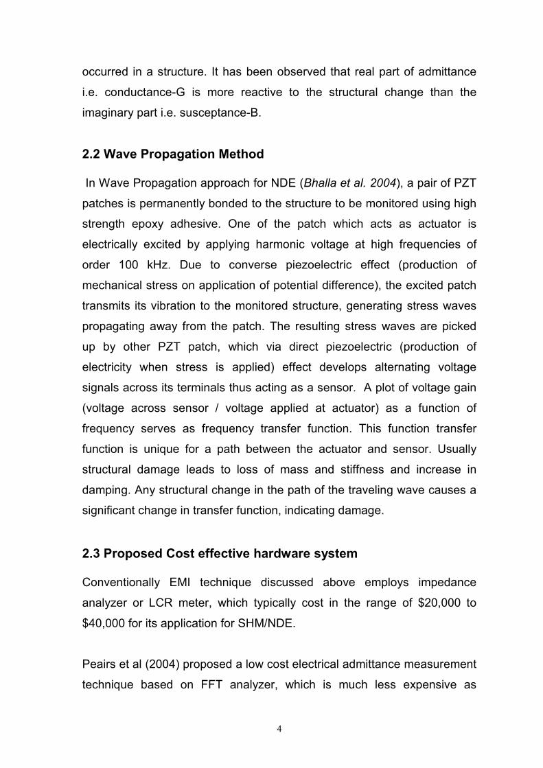
compared to LCR meter. Figure 2.3(a) shows the electrical circuit

employed by Peairs and co-workers. It essentially consisted of a small

resistance (10-20Ώ) connected in series with the PZT patch bonded to the

structure to be monitored. Upon applying the input voltage Vi and

measuring the output voltage Vo the total admittance can be calculated

using the relation given by:

A=Vo/ViR

Figure 2.3(a) Circuit for approximating PZT admittance (Peairs et al. 2004)

Typically an FFT analyzer costs in excess of $10,000 and the above

relation gave total admittance which is not much sensitive to damage.

Conventionally used LCR meter gave the values of Real admittance-G and

imaginary admittance separately and as stated above it is observed that

the real admittance is more sensitive to damage. By using the total

admittance the change in frequency response function reduces

considerably which have been successfully demonstrated in the

experiment conducted.

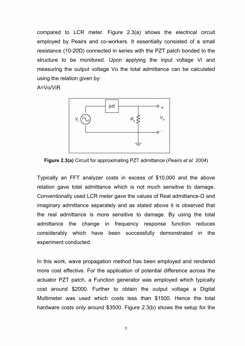
In this work, wave propagation method has been employed and rendered

more cost effective. For the application of potential difference across the

actuator PZT patch, a Function generator was employed which typically

cost around $2000. Further to obtain the output voltage a Digital

Multimeter was used which costs less than $1500. Hence the total

hardware costs only around $3500. Figure 2.3(b) shows the setup for the

6

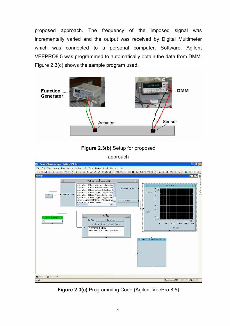
proposed approach. The frequency of the imposed signal was

incrementally varied and the output was received by Digital Multimeter

which was connected to a personal computer. Software, Agilent

VEEPRO8.5 was programmed to automatically obtain the data from DMM.

Figure 2.3(c) shows the sample program used.

Figure 2.3(b) Setup for proposed

approach

Figure 2.3(c) Programming Code (Agilent VeePro 8.5)

7

Chapter 3

Tests Results and Analysis

3.1 Experimental Details

The test specimen consisted of an aluminum beam having dimensions

600*25*5. Two PZT patches were bonded to the sample using standard

araldite epoxy adhesive. One of the PZT patch was used as actuator and

other as sensor. The actuator PZT was excited by applying a sinusoidal

voltage of RMS 5V by means of a function generator FG-702C (µ-TEC

Electronic Measuring Instruments). The excitation frequency was varied

from 150 kHz to 160 kHz. Due to converse piezoelectric effect the vibration

was passed to the monitored specimen. The resulting vibration was picked

by the sensor patch, which developed a voltage across its terminals

because of direct piezoelectric effect and was measured using a Digital

Multimeter (Agilent 34411A Digital Multimeter). Measurements were made

at an interval of 200Hz. A plot of voltage gain served as frequency

response function. Damage was introduced by drilling a hole of diameter

5mm in the middle of the specimen. After inducing the damage the

frequency transfer function was recorded again. To quantify the deviation

in the transfer function, damage metric was defined as follow:

%100)(

2

1

2

12×

−=

∑∑

G

GGM

M = damage metric (Root Mean Square Deviation)

G1 = Baseline measurement

G2 = After Damage measurement

In order to verify the new low cost measuring method the test specimen

was also tested using EMI (Electro Mechanical Impedance) method and

Peairs low cost electrical admittance technique (Peairs et al 2004). The

8

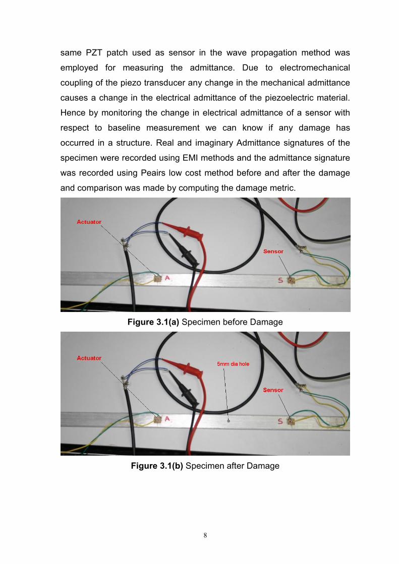
same PZT patch used as sensor in the wave propagation method was

employed for measuring the admittance. Due to electromechanical

coupling of the piezo transducer any change in the mechanical admittance

causes a change in the electrical admittance of the piezoelectric material.

Hence by monitoring the change in electrical admittance of a sensor with

respect to baseline measurement we can know if any damage has

occurred in a structure. Real and imaginary Admittance signatures of the

specimen were recorded using EMI methods and the admittance signature

was recorded using Peairs low cost method before and after the damage

and comparison was made by computing the damage metric.

Figure 3.1(a) Specimen before Damage

Figure 3.1(b) Specimen after Damage

9

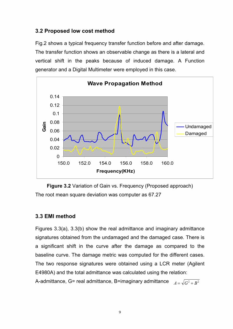
3.2 Proposed low cost method

Fig.2 shows a typical frequency transfer function before and after damage.

The transfer function shows an observable change as there is a lateral and

vertical shift in the peaks because of induced damage. A Function

generator and a Digital Multimeter were employed in this case.

Wave Propagation Method

0

0.02

0.04

0.06

0.08

0.1

0.12

0.14

150.0 152.0 154.0 156.0 158.0 160.0

Frequency(KHz)

Gain

Undamaged

Damaged

Figure 3.2 Variation of Gain vs. Frequency (Proposed approach)

The root mean square deviation was computer as 67.27

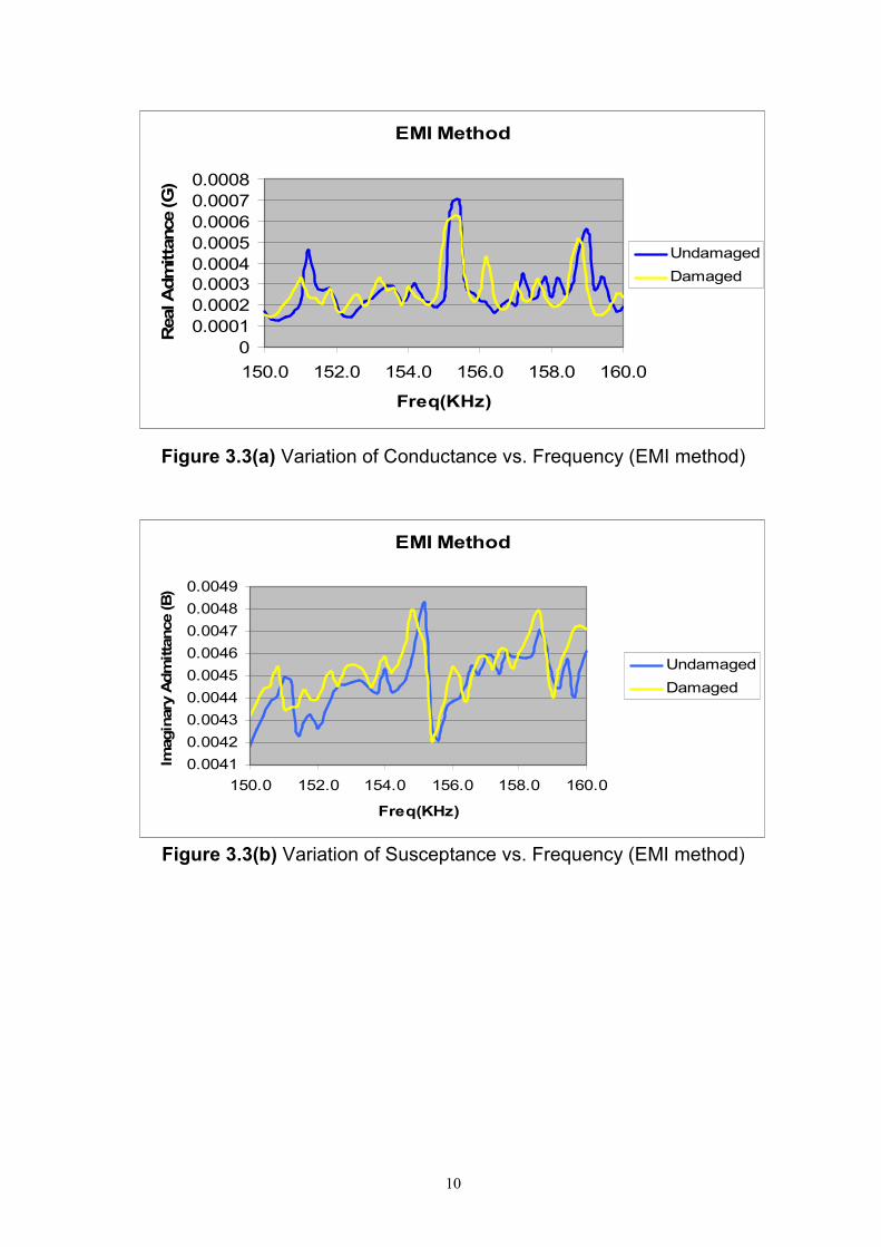
3.3 EMI method

Figures 3.3(a), 3.3(b) show the real admittance and imaginary admittance

signatures obtained from the undamaged and the damaged case. There is

a significant shift in the curve after the damage as compared to the

baseline curve. The damage metric was computed for the different cases.

The two response signatures were obtained using a LCR meter (Agilent

E4980A) and the total admittance was calculated using the relation:

A-admittance, G= real admittance, B=imaginary admittance 22 BGA +=

10

EMI Method

0

0.0001

0.0002

0.00030.0004

0.0005

0.0006

0.0007

0.0008

150.0 152.0 154.0 156.0 158.0 160.0

Freq(KHz)

Real A

dm

itta

nce (G

)

Undamaged

Damaged

Figure 3.3(a) Variation of Conductance vs. Frequency (EMI method)

EMI Method

0.0041

0.0042

0.0043

0.0044

0.0045

0.0046

0.0047

0.0048

0.0049

150.0 152.0 154.0 156.0 158.0 160.0

Freq(KHz)

Imagin

ary

Adm

itta

nce (B

)

Undamaged

Damaged

Figure 3.3(b) Variation of Susceptance vs. Frequency (EMI method)

11

EMI Method

0.0041

0.0042

0.0043

0.0044

0.0045

0.0046

0.0047

0.0048

0.0049

0.005

150.0 152.0 154.0 156.0 158.0 160.0

Freq(KHz)

Adm

itta

nce(A

)

Undamaged

Damaged

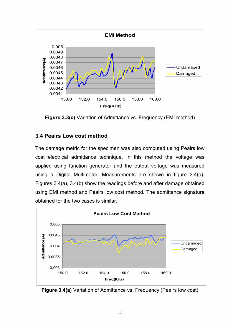
Figure 3.3(c) Variation of Admittance vs. Frequency (EMI method)

3.4 Peairs Low cost method

The damage metric for the specimen was also computed using Peairs low

cost electrical admittance technique. In this method the voltage was

applied using function generator and the output voltage was measured

using a Digital Multimeter. Measurements are shown in figure 3.4(a).

Figures 3.4(a), 3.4(b) show the readings before and after damage obtained

using EMI method and Peairs low cost method. The admittance signature

obtained for the two cases is similar.

Peairs Low Cost Method

0.003

0.0035

0.004

0.0045

0.005

150.0 152.0 154.0 156.0 158.0 160.0

Freq(KHz)

Adm

itta

nce (A

)

Undamaged

Damaged

Figure 3.4(a) Variation of Admittance vs. Frequency (Peairs low cost)

12

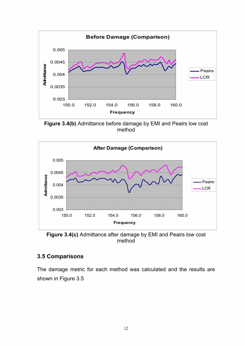
Before Damage (Comparison)

0.003

0.0035

0.004

0.0045

0.005

150.0 152.0 154.0 156.0 158.0 160.0

Frequency

Adm

itta

nce

Peairs

LCR

Figure 3.4(b) Admittance before damage by EMI and Peairs low cost method

After Damage (Comparison)

0.003

0.0035

0.004

0.0045

0.005

150.0 152.0 154.0 156.0 158.0 160.0

Frequency

Ad

mit

tan

ce

Peairs

LCR

Figure 3.4(c) Admittance after damage by EMI and Peairs low cost method

3.5 Comparisons

The damage metric for each method was calculated and the results are

shown in Figure 3.5

13

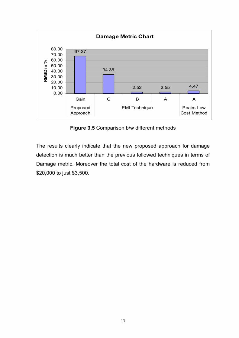
Damage Metric Chart

67.27

34.35

2.52 2.55 4.47

0.00

10.00

20.00

30.00

40.00

50.00

60.00

70.00

80.00

Gain G B A A

Proposed

Approach

EMI Technique Peairs Low

Cost Method

RM

SD

in %

Figure 3.5 Comparison b/w different methods

The results clearly indicate that the new proposed approach for damage

detection is much better than the previous followed techniques in terms of

Damage metric. Moreover the total cost of the hardware is reduced from

$20,000 to just $3,500.

14

Chapter 4

Conclusions

4.1 Conclusion

This report proposes a new low-cost technique for non destructive health

monitoring of structures suitable for widespread industrial applications.

This technique makes use of a function generator and a Digital Multimeter,

which are commonly available in structural laboratories, and is much more

cost-effective as compared to the conventionally employed impedance

analyzers/LCR meters as well as the FFT analyzers. The test result

indicates that the new proposed approach is more able to detect any

damage as compared to traditional methods.

4.2 Limitations and Sources of error

One of the limitations in the test technique was the use of old function

generator which did not connect to a computer. There fore the frequency at

function generator had to be set manually which made the process time

consuming and slow. Though the limitation of function generator the use of

Digital Multimeter which has inbuilt storage capacity was able to record the

readings both frequency and output voltage and reduced the error. Errors

because of noise were inevitable.

The testing process can be made more time efficient by employing a digital

function generator and programming the two equipments together so that

the whole procedure is made automatic and faster.

15

References:

• Agilent Technologies (2008). http://www.agilent.com

• Bhalla, S., Soh, C. K. And Liu, Z. (2005) Wave propagation

approach for NDE using surface bonded piezoceramics. NDT & E

International 38, 143-150.

• Bhalla, S. and Soh, C. k. (2004) Structural health monitoring by

piezo-admittance transducers. II: Applications. Journal of Aerospace

Engineering ASCE 17, 154-165.

• Daniel M. Peairs, Gyuhae Park, and Daniel J. Inman Low Cost

Admittance Monitoring Using Smart Materials

• Peairs, D., Park, G., Inman, D.J. (2002a) “Self-Healing Bolted Joint

Analysis,” Proceedings of 20th International Modal Analysis

Conference, February 4-7, Los Angles, CA.

• Peairs, D. M., Park, G. and Inman, D. J. (2004). “Improving

accessibility of the 17 impedance-based structural health monitoring

method.” Journal of Intelligent Material 18 Systems and Structures,

15, 129-39.

• Raju, V., (1998) “Implementing Impedance-Based Health Monitoring

Technique,” Master’s thesis, Virginia Polytechnic Institute and State

University, Blacksburg, VA.

• Soh, C. K. and Bhalla, S. (2005) Calibration of piezo-admittance

transducers for strength prediction and damage assessment of

concrete. Smart Materials and Structures 14, 671-684.

16

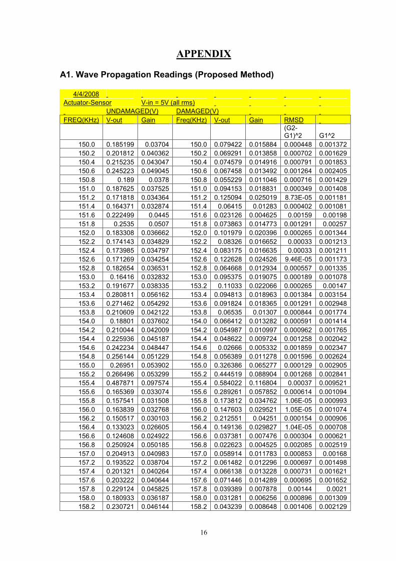
APPEDIX A1. Wave Propagation Readings (Proposed Method)

4/4/2008

Actuator-Sensor V-in = 5V (all rms)

UNDAMAGED(V) DAMAGED(V)

FREQ(KHz) V-out Gain Freq(KHz) V-out Gain RMSD

(G2-G1)^2 G1^2

150.0 0.185199 0.03704 150.0 0.079422 0.015884 0.000448 0.001372

150.2 0.201812 0.040362 150.2 0.069291 0.013858 0.000702 0.001629

150.4 0.215235 0.043047 150.4 0.074579 0.014916 0.000791 0.001853

150.6 0.245223 0.049045 150.6 0.067458 0.013492 0.001264 0.002405

150.8 0.189 0.0378 150.8 0.055229 0.011046 0.000716 0.001429

151.0 0.187625 0.037525 151.0 0.094153 0.018831 0.000349 0.001408

151.2 0.171818 0.034364 151.2 0.125094 0.025019 8.73E-05 0.001181

151.4 0.164371 0.032874 151.4 0.06415 0.01283 0.000402 0.001081

151.6 0.222499 0.0445 151.6 0.023126 0.004625 0.00159 0.00198

151.8 0.2535 0.0507 151.8 0.073863 0.014773 0.001291 0.00257

152.0 0.183308 0.036662 152.0 0.101979 0.020396 0.000265 0.001344

152.2 0.174143 0.034829 152.2 0.08326 0.016652 0.00033 0.001213

152.4 0.173985 0.034797 152.4 0.083175 0.016635 0.00033 0.001211

152.6 0.171269 0.034254 152.6 0.122628 0.024526 9.46E-05 0.001173

152.8 0.182654 0.036531 152.8 0.064668 0.012934 0.000557 0.001335

153.0 0.16416 0.032832 153.0 0.095375 0.019075 0.000189 0.001078

153.2 0.191677 0.038335 153.2 0.11033 0.022066 0.000265 0.00147

153.4 0.280811 0.056162 153.4 0.094813 0.018963 0.001384 0.003154

153.6 0.271462 0.054292 153.6 0.091824 0.018365 0.001291 0.002948

153.8 0.210609 0.042122 153.8 0.06535 0.01307 0.000844 0.001774

154.0 0.18801 0.037602 154.0 0.066412 0.013282 0.000591 0.001414

154.2 0.210044 0.042009 154.2 0.054987 0.010997 0.000962 0.001765

154.4 0.225936 0.045187 154.4 0.048622 0.009724 0.001258 0.002042

154.6 0.242234 0.048447 154.6 0.02666 0.005332 0.001859 0.002347

154.8 0.256144 0.051229 154.8 0.056389 0.011278 0.001596 0.002624

155.0 0.26951 0.053902 155.0 0.326386 0.065277 0.000129 0.002905

155.2 0.266496 0.053299 155.2 0.444519 0.088904 0.001268 0.002841

155.4 0.487871 0.097574 155.4 0.584022 0.116804 0.00037 0.009521

155.6 0.165369 0.033074 155.6 0.289261 0.057852 0.000614 0.001094

155.8 0.157541 0.031508 155.8 0.173812 0.034762 1.06E-05 0.000993

156.0 0.163839 0.032768 156.0 0.147603 0.029521 1.05E-05 0.001074

156.2 0.150517 0.030103 156.2 0.212551 0.04251 0.000154 0.000906

156.4 0.133023 0.026605 156.4 0.149136 0.029827 1.04E-05 0.000708

156.6 0.124608 0.024922 156.6 0.037381 0.007476 0.000304 0.000621

156.8 0.250924 0.050185 156.8 0.022623 0.004525 0.002085 0.002519

157.0 0.204913 0.040983 157.0 0.058914 0.011783 0.000853 0.00168

157.2 0.193522 0.038704 157.2 0.061482 0.012296 0.000697 0.001498

157.4 0.201321 0.040264 157.4 0.066138 0.013228 0.000731 0.001621

157.6 0.203222 0.040644 157.6 0.071446 0.014289 0.000695 0.001652

157.8 0.229124 0.045825 157.8 0.039389 0.007878 0.00144 0.0021

158.0 0.180933 0.036187 158.0 0.031281 0.006256 0.000896 0.001309

158.2 0.230721 0.046144 158.2 0.043239 0.008648 0.001406 0.002129

17

158.4 0.250758 0.050152 158.4 0.042229 0.008446 0.001739 0.002515

158.6 0.255124 0.051025 158.6 0.054185 0.010837 0.001615 0.002604

158.8 0.187873 0.037575 158.8 0.161286 0.032257 2.83E-05 0.001412

159.0 0.150828 0.030166 159.0 0.290041 0.058008 0.000775 0.00091

159.2 0.189096 0.037819 159.2 0.164949 0.03299 2.33E-05 0.00143

159.4 0.298602 0.05972 159.4 0.097594 0.019519 0.001616 0.003567

159.6 0.529479 0.105896 159.6 0.083091 0.016618 0.00797 0.011214

159.8 0.400724 0.080145 159.8 0.084586 0.016917 0.003998 0.006423

160.0 0.358569 0.071714 160.0 0.094885 0.018977 0.002781 0.005143

0.051675 0.114188

RMSD= 67.27121

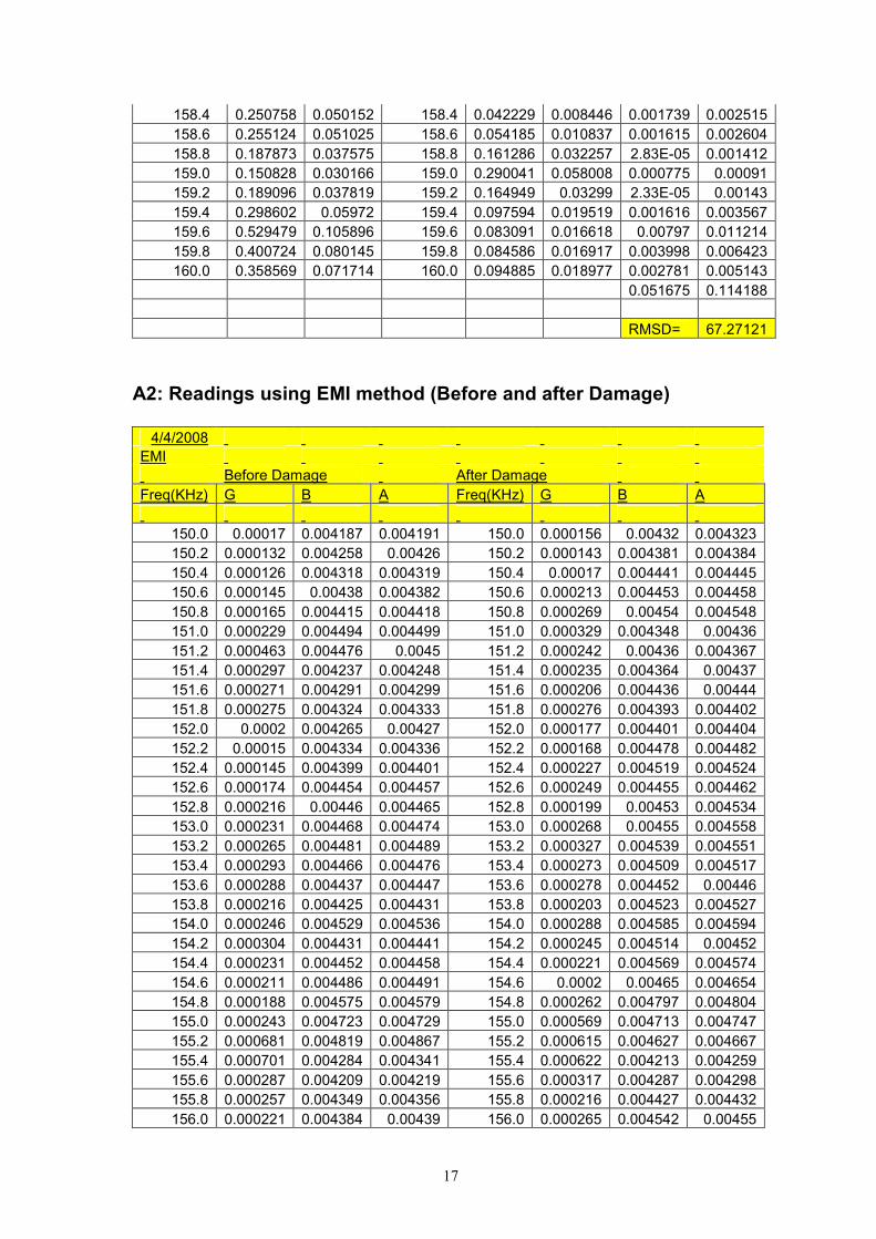
A2: Readings using EMI method (Before and after Damage)

4/4/2008

EMI

Before Damage After Damage

Freq(KHz) G B A Freq(KHz) G B A

150.0 0.00017 0.004187 0.004191 150.0 0.000156 0.00432 0.004323

150.2 0.000132 0.004258 0.00426 150.2 0.000143 0.004381 0.004384

150.4 0.000126 0.004318 0.004319 150.4 0.00017 0.004441 0.004445

150.6 0.000145 0.00438 0.004382 150.6 0.000213 0.004453 0.004458

150.8 0.000165 0.004415 0.004418 150.8 0.000269 0.00454 0.004548

151.0 0.000229 0.004494 0.004499 151.0 0.000329 0.004348 0.00436

151.2 0.000463 0.004476 0.0045 151.2 0.000242 0.00436 0.004367

151.4 0.000297 0.004237 0.004248 151.4 0.000235 0.004364 0.00437

151.6 0.000271 0.004291 0.004299 151.6 0.000206 0.004436 0.00444

151.8 0.000275 0.004324 0.004333 151.8 0.000276 0.004393 0.004402

152.0 0.0002 0.004265 0.00427 152.0 0.000177 0.004401 0.004404

152.2 0.00015 0.004334 0.004336 152.2 0.000168 0.004478 0.004482

152.4 0.000145 0.004399 0.004401 152.4 0.000227 0.004519 0.004524

152.6 0.000174 0.004454 0.004457 152.6 0.000249 0.004455 0.004462

152.8 0.000216 0.00446 0.004465 152.8 0.000199 0.00453 0.004534

153.0 0.000231 0.004468 0.004474 153.0 0.000268 0.00455 0.004558

153.2 0.000265 0.004481 0.004489 153.2 0.000327 0.004539 0.004551

153.4 0.000293 0.004466 0.004476 153.4 0.000273 0.004509 0.004517

153.6 0.000288 0.004437 0.004447 153.6 0.000278 0.004452 0.00446

153.8 0.000216 0.004425 0.004431 153.8 0.000203 0.004523 0.004527

154.0 0.000246 0.004529 0.004536 154.0 0.000288 0.004585 0.004594

154.2 0.000304 0.004431 0.004441 154.2 0.000245 0.004514 0.00452

154.4 0.000231 0.004452 0.004458 154.4 0.000221 0.004569 0.004574

154.6 0.000211 0.004486 0.004491 154.6 0.0002 0.00465 0.004654

154.8 0.000188 0.004575 0.004579 154.8 0.000262 0.004797 0.004804

155.0 0.000243 0.004723 0.004729 155.0 0.000569 0.004713 0.004747

155.2 0.000681 0.004819 0.004867 155.2 0.000615 0.004627 0.004667

155.4 0.000701 0.004284 0.004341 155.4 0.000622 0.004213 0.004259

155.6 0.000287 0.004209 0.004219 155.6 0.000317 0.004287 0.004298

155.8 0.000257 0.004349 0.004356 155.8 0.000216 0.004427 0.004432

156.0 0.000221 0.004384 0.00439 156.0 0.000265 0.004542 0.00455

18

156.2 0.000211 0.004399 0.004404 156.2 0.000427 0.004499 0.004519

156.4 0.000165 0.00446 0.004463 156.4 0.000243 0.004386 0.004393

156.6 0.000191 0.004544 0.004548 156.6 0.00018 0.004493 0.004496

156.8 0.000224 0.004504 0.00451 156.8 0.000203 0.004581 0.004585

157.0 0.000201 0.004591 0.004596 157.0 0.000308 0.004583 0.004593

157.2 0.000352 0.004583 0.004596 157.2 0.000225 0.004529 0.004534

157.4 0.000234 0.004508 0.004514 157.4 0.000229 0.004613 0.004619

157.6 0.000241 0.004603 0.004609 157.6 0.000322 0.004616 0.004627

157.8 0.000334 0.004584 0.004596 157.8 0.000241 0.004533 0.004539

158.0 0.000237 0.004585 0.004591 158.0 0.000194 0.004601 0.004605

158.2 0.00033 0.004582 0.004594 158.2 0.000196 0.004666 0.00467

158.4 0.000249 0.0046 0.004606 158.4 0.000237 0.004751 0.004757

158.6 0.000295 0.004707 0.004716 158.6 0.000422 0.004792 0.004811

158.8 0.000476 0.004636 0.004661 158.8 0.000507 0.004593 0.004621

159.0 0.000555 0.004487 0.004521 159.0 0.000269 0.004403 0.004411

159.2 0.000276 0.004443 0.004451 159.2 0.000166 0.004541 0.004544

159.4 0.000332 0.004575 0.004587 159.4 0.000154 0.004631 0.004634

159.6 0.000244 0.004405 0.004412 159.6 0.000178 0.004711 0.004714

159.8 0.000168 0.004525 0.004528 159.8 0.000255 0.004723 0.004729

160.0 0.000189 0.004608 0.004612 160.0 0.000239 0.004708 0.004714

RMSD(%) G 34.3533

B 2.520366

A 2.546461

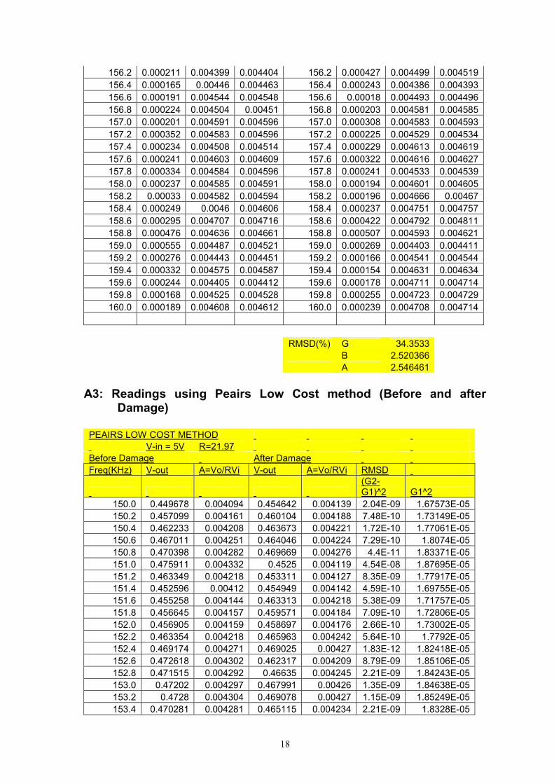
A3: Readings using Peairs Low Cost method (Before and after Damage) PEAIRS LOW COST METHOD

V-in = 5V R=21.97

Before Damage After Damage

Freq(KHz) V-out A=Vo/RVi V-out A=Vo/RVi RMSD

(G2-G1)^2 G1^2

150.0 0.449678 0.004094 0.454642 0.004139 2.04E-09 1.67573E-05

150.2 0.457099 0.004161 0.460104 0.004188 7.48E-10 1.73149E-05

150.4 0.462233 0.004208 0.463673 0.004221 1.72E-10 1.77061E-05

150.6 0.467011 0.004251 0.464046 0.004224 7.29E-10 1.8074E-05

150.8 0.470398 0.004282 0.469669 0.004276 4.4E-11 1.83371E-05

151.0 0.475911 0.004332 0.4525 0.004119 4.54E-08 1.87695E-05

151.2 0.463349 0.004218 0.453311 0.004127 8.35E-09 1.77917E-05

151.4 0.452596 0.00412 0.454949 0.004142 4.59E-10 1.69755E-05

151.6 0.455258 0.004144 0.463313 0.004218 5.38E-09 1.71757E-05

151.8 0.456645 0.004157 0.459571 0.004184 7.09E-10 1.72806E-05

152.0 0.456905 0.004159 0.458697 0.004176 2.66E-10 1.73002E-05

152.2 0.463354 0.004218 0.465963 0.004242 5.64E-10 1.7792E-05

152.4 0.469174 0.004271 0.469025 0.00427 1.83E-12 1.82418E-05

152.6 0.472618 0.004302 0.462317 0.004209 8.79E-09 1.85106E-05

152.8 0.471515 0.004292 0.46635 0.004245 2.21E-09 1.84243E-05

153.0 0.47202 0.004297 0.467991 0.00426 1.35E-09 1.84638E-05

153.2 0.4728 0.004304 0.469078 0.00427 1.15E-09 1.85249E-05

153.4 0.470281 0.004281 0.465115 0.004234 2.21E-09 1.8328E-05

19

153.6 0.468035 0.004261 0.46135 0.0042 3.7E-09 1.81534E-05

153.8 0.470993 0.004288 0.466385 0.004246 1.76E-09 1.83835E-05

154.0 0.478969 0.00436 0.452765 0.004122 5.69E-08 1.90115E-05

154.2 0.470138 0.00428 0.465315 0.004236 1.93E-09 1.83169E-05

154.4 0.471673 0.004294 0.450866 0.004104 3.59E-08 1.84366E-05

154.6 0.476013 0.004333 0.453153 0.004125 4.33E-08 1.87775E-05

154.8 0.484593 0.004411 0.466085 0.004243 2.84E-08 1.94605E-05

155.0 0.49742 0.004528 0.46119 0.004198 1.09E-07 2.05044E-05

155.2 0.481553 0.004384 0.445355 0.004054 1.09E-07 1.92171E-05

155.4 0.443338 0.004036 0.407091 0.003706 1.09E-07 1.62881E-05

155.6 0.450546 0.004101 0.42243 0.003846 6.55E-08 1.6822E-05

155.8 0.462911 0.004214 0.434996 0.00396 6.46E-08 1.7758E-05

156.0 0.467733 0.004258 0.444187 0.004044 4.59E-08 1.81299E-05

156.2 0.467823 0.004259 0.44163 0.00402 5.69E-08 1.81369E-05

156.4 0.474685 0.004321 0.430397 0.003918 1.63E-07 1.86729E-05

156.6 0.481158 0.00438 0.462524 0.004211 2.88E-08 1.91856E-05

156.8 0.476072 0.004334 0.45493 0.004141 3.7E-08 1.87821E-05

157.0 0.485056 0.004416 0.449767 0.004094 1.03E-07 1.94977E-05

157.2 0.478445 0.004355 0.4402 0.004007 1.21E-07 1.89699E-05

157.4 0.478011 0.004351 0.451083 0.004106 6.01E-08 1.89354E-05

157.6 0.48592 0.004423 0.454944 0.004142 7.95E-08 1.95673E-05

157.8 0.479877 0.004368 0.444571 0.004047 1.03E-07 1.90836E-05

158.0 0.48642 0.004428 0.447245 0.004071 1.27E-07 1.96076E-05

158.2 0.483272 0.004399 0.479142 0.004362 1.41E-09 1.93546E-05

158.4 0.48683 0.004432 0.453028 0.004124 9.47E-08 1.96406E-05

158.6 0.494638 0.004503 0.459895 0.004187 1E-07 2.02757E-05

158.8 0.476219 0.004335 0.464079 0.004225 1.22E-08 1.87937E-05

159.0 0.457072 0.004161 0.447008 0.004069 8.39E-09 1.73129E-05

159.2 0.468708 0.004267 0.463459 0.004219 2.28E-09 1.82056E-05

159.4 0.476558 0.004338 0.477088 0.004343 2.33E-11 1.88205E-05

159.6 0.469137 0.004271 0.486737 0.004431 2.57E-08 1.82389E-05

159.8 0.481023 0.004379 0.482326 0.004391 1.41E-10 1.91748E-05

160.0 0.488465 0.004447 0.484441 0.00441 1.34E-09 1.97728E-05

1.88E-06 0.000941056

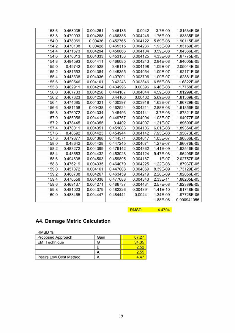
RMSD 4.4704

A4. Damage Metric Calculation RMSD %

Proposed Approach Gain 67.27

EMI Technique G 34.35

B 2.52

A 2.55

Peairs Low Cost Method A 4.47