FEDERAL RESERVE BANK OF SAN FRANCISCO

WORKING PAPER SERIES

Working Paper 2008-19 http://www.frbsf.org/publications/economics/papers/2008/wp08-19bk.pdf

The views in this paper are solely the responsibility of the authors and should not be interpreted as reflecting the views of the Federal Reserve Bank of San Francisco or the Board of Governors of the Federal Reserve System.

Happiness, Unhappiness, and Suicide: An Empirical Assessment

Mary C. Daly

Federal Reserve Bank of San Francisco

Daniel J. Wilson Federal Reserve Bank of San Francisco

August 2008

Happiness, Unhappiness, and Suicide: An Empirical Assessment

Mary C. Dalya and Daniel J. Wilsona

Economic Research Department Federal Reserve Bank of San Francisco

101 Market Street, Mail Stop 1130 San Francisco, CA 94610

Prepared for the Annual Meetings of the European Economic Association Invited Session on Status and Utility

August 27-31, 2008

First Draft: August 2008

Please cite as: Daly, Mary C., Daniel J. Wilson. “Happiness, Unhappiness, and Suicide: An Empirical Assessment.” Federal Reserve Bank of San Francisco Working Paper, 2008-18. a Federal Reserve Bank of San Francisco Corresponding author’s email: Daniel.Wilson@sf.frb.org This paper benefited from helpful comments from Heather Royer. We thank Norm Johnson at the U.S. Census Bureau for providing us with the regression estimates reported in this paper involving the National Longitudinal Mortality Study. We also thank Thomas O’Connell and Joyce Kwok for excellent research assistance. Research results and conclusions expressed are those of the authors and do not necessarily indicate concurrence by the Federal Reserve Bank of San Francisco, the Federal Reserve System, or the U.S. Census Bureau.

1

Happiness, Unhappiness, and Suicide: An Empirical Assessment

Abstract

The use of subjective well-being (SWB) data for investigating the nature of individual preferences has increased tremendously in recent years. There has been much debate about the cross-sectional and time-series patterns found in these data, particularly with respect to the relationship between SWB and relative status. Part of this debate concerns how well SWB data measures true utility or preferences. In a recent paper, Daly, Wilson, and Johnson (2007) propose using data on suicide as a revealed preference (outcome-based) measure of well-being and find strong evidence that reference-group income negatively affects suicide risk. In this paper, we compare and contrast the empirical patterns of SWB and suicide data. We find that the two have very little in common in aggregate data (time series and cross-sectional), but have a strikingly strong relationship in terms of their determinants in individual-level, multivariate regressions. This latter result cross-validates suicide and SWB micro data as useful and complementary indicators of latent utility.

Keywords: Happiness and unhappiness trends, suicide, utility, relative income.

JEL Codes: I31, D6, H0, J0

2

Happiness, Unhappiness, and Suicide: An Empirical Assessment

I. Introduction

Over the past decade economists have dramatically increased their interest in and use of subjective well-

being data to track individual and aggregate welfare and to examine issues related to preference formation

and utility. Empirical research has included comparing subjective assessments of well-being over time

(e.g., time series patterns in happiness, unhappiness, life-satisfaction) and analyzing the individual and

group-specific correlates of these measures in the cross-section. The work has produced intriguing

results—aggregate happiness does not rise monotonically with income (Easterlin 1995, Blanchflower and

Oswald 2004), individuals care about their own and others’ income (Luttmer 2005; McBride 2001; Clark

and Oswald 1996; Ferrer-i-Carbonell 2005), and preferences seem to adapt to the environment (Gardner

and Oswald 2007). Despite widespread interest in these results outside of economics, they have been slow

to affect mainstream economic theory and its application.

An important barrier to greater acceptance of the findings from subjective well-being research has been

concerns about data quality. Subjective survey questions, by design, elicit information about individuals’

feelings, attitudes, opinions, and views. Critics argue that these features introduce systematic and non-

systematic measurement errors that make it difficult to compare answers to such questions over time or

across individuals (see Bertrand and Mullainathan 2001 for a broad critique of subjective survey data). In

the subjective well-being surveys, for example, in which respondents are asked to “rate” or “score” their

happiness or life satisfaction, errors can arise from language ambiguities (respondents may not all agree

on the exact meaning of terms like “happiness” and “life satisfaction”), scale comparability (one person’s

“very satisfied” may be higher, lower, or equal to another person’s “satisfied”), ambiguity regarding the

time period over which respondents base their answers, respondent candidness, and the difficulty of

drawing cardinal inferences from ordinal survey responses.1 These problems have prompted some to

discount the results from subjective well-being research and have left a larger number unconvinced of the

robustness of the findings.

At issue with each of these concerns is whether subjective well-being reports accurately capture the

underlying latent variable that is utility. Since we are not able to observe the latent variable, debates

about whether it can be accurately measured are hard to resolve. This has led researchers to seek

alternative, outcome-based (i.e., non-subjective) sources of data to verify or reject the findings from 1Bertrand and Mullainathan (2001) argue that even when questions are well-stated and well-understood, respondents may make cognitive errors that bias their answers and limit their usefulness as dependent variables in outcome studies.

3

subjective surveys. These alternative data sources include laboratory experimental work and naturally

occurring phenomena. Experiments have the advantage of controlling the environment so as to reduce

measurement error but have the disadvantage of small sample sizes and contrived situations. Outcome-

based studies, such as those looking at mortality and status (Miller and Paxson 2006) or the consumption

of positional goods (Carlsson, Johansson-Stenman, and Martinsson 2007), have the advantage of tracking

actual occurrences, rather than attitudes or laboratory responses, but carry the disadvantage of embodying

many potential determinants unrelated to preferences.

In the vein of outcome-based studies, Daly, Wilson, and Johnson (2007) consider whether suicide data

can be used to address questions regarding interdependent preferences. They argue that suicide represents

a revealed choice that can be considered a direct measure of well-being. Using individual-level

longitudinal data, they find that relative income does matter for suicide risk, confirming results from

subjective well-being and experimental work. An obvious concern regarding suicide data, however, is

that the preferences of suicide victims, who arguably are at the extreme lower tail of the well-being

distribution, may not be representative of the overall population.

In this paper we attempt to resolve some of the uncertainty regarding the reasonableness of the subjective

well-being and suicide data by performing a type of cross-validation exercise across the two data types.

At the root of our study is an interest in knowing whether the two data series capture the latent variable on

well-being that would allow one to infer preferences from their relationships with other variables. To

move toward an answer, we assess how subjective well-being and suicide data match up over a range of

analyses. We look first at the aggregate patterns, both in the time-series and in population-based cross-

sections. We then consider micro-multivariate patterns in the data by comparing the results from parallel

individual-level regressions.

Under the principles of cross-validation, failure to find a systematic relationship between these data

means we keep searching, since a negative result could be driven by either or both of the series. If,

however, we find a strong relationship across these sources, then we have additional support for the

notion that the results reflect true preferences of the general population. Previewing our results, we find

essentially no relationship between the suicide rate and the subjective well-being data in the aggregate

time series patterns. We find a weak relationship between suicide in the aggregate cross-sectional results,

but it is inconsistent across variables. In contrast, at the micro level, we find a strikingly strong

relationship between the relative risks on the variables associated with greater suicide risk and higher

likelihood of unhappiness. Our results suggest that while researchers should be cautious about inferences

4

based on time series data from SWB surveys or suicide rates, the findings from micro data on SWB and

suicide appear to be quite reflective of typical preferences in society.

II. Data

Our analysis is based on information from two main sources. The data on subjective well-being come

from the General Social Survey (GSS). The GSS is a survey of American demographics, behaviors,

attitudes, and opinions, administered since 1972 by the National Opinion Research Center out of the

University of Chicago. It is structured to be a representative sample of the U.S. population; it was

administered to about 1,500 respondents per year from 1972-1993 (excluding 1979, 1981, and 1992),

3,000 from 1994 through 2004, and about 4,500 respondents in 2006.2 Our analysis relies on a wide

range of variables from the GSS including demographic and income variables. Our key interest is the

question on subjective well-being. This question reads: “Taken all together, how would you say things

are these days—would you say that you are very happy, pretty happy, or not too happy?” To underscore

the purely ordinal content of the responses and avoid letting any connotations of the answer choices

influence how we treat the data or discuss the results, we simply recode the responses “very happy,”

“pretty happy,” and “not too happy” as “high”, “medium”, and “low,” respectively.

Results for suicide come from three different sources, all of which are based on U.S. Death Certificate

data. The time series of U.S. suicide rates, available from 1950 to 2006, come from U.S. Vital Statistics

(VS). The VS data are useful for plotting trends but have limited demographic information (age, race,

gender) so are not useful for more detailed comparisons. For more detailed analyses we rely on two

additional sources that we have used in other work (Daly, Wilson, and Johnson 2007). The first is the

Mortality Detail Files (MDF), which are produced by the National Center for Health Statistics and

distributed by the Inter-university Consortium for Political and Social Research (ICPSR). For any given

year, the MDF is essentially the data from all death certificates recorded in the United States in that year

(see U.S. Department of Health and Human Services 1992). These data include a variety of important

demographic and employment-related variables, and so we rely on them for cross-sectional descriptive

analysis. Finally, we use the National Longitudinal Mortality Study (NLMS) for individual level

regressions. The NLMS consists of files from the Current Population Surveys (CPS) from 1978 to 1998,

matched to the National Death Index (NDI), a national database containing the universe of U.S. death

certificates. The matching process appends to individual CPS records (1) whether the person has died

within the follow-up period (1979 through 1998), (2) date of death (if deceased), and (3) cause of death (if

2 Note that only about one half the total respondents were asked about their happiness from 2002 through 2004, and about two-thirds were asked in 2006.

5

deceased). Importantly, suicide rates computed from VS, the MDF, and the NLMS are very similar and

assure us that the data sources are interchangeable for research purposes.

III. Aggregate Patterns in Subjective Well-Being and Suicide Data

Time Series

To get a sense of how subjective well-being and suicide line up it is useful to look at a simple time series

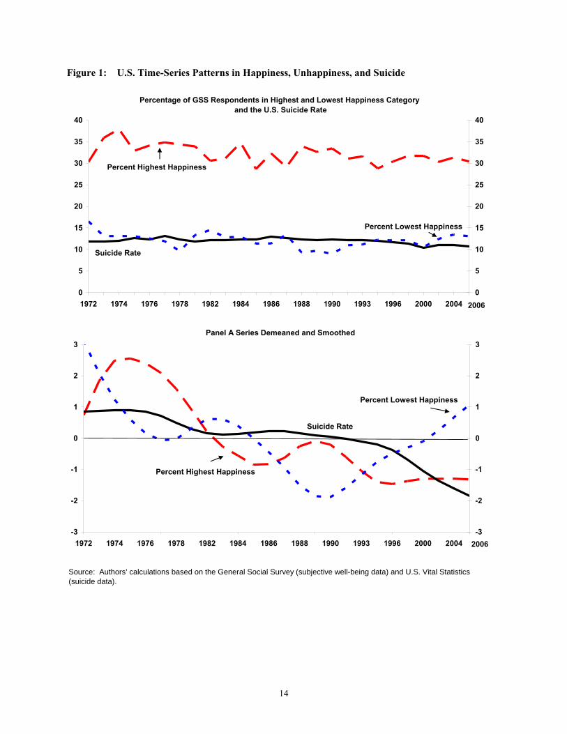
plot. Figure 1, panel A shows three series: (1) percent highest happiness – the percent of respondents in

the high happiness category, (2) percent lowest happiness– the percent in the low category, and (3) the

suicide rate – the number of suicides per 100,000 population. The data span the period from 1972 to

2006. The most striking pattern in Figure 1 is the relative constancy of all three series. Over the period

of more than 30 years, the proportions of reported happiness, unhappiness, and suicide have hardly

changed.3 On average over the period, about 30% of GSS respondents reported being in the highest of the

three happiness categories and about 14% reported being in the lowest category. The average suicide rate

was 12 per 100,000.

The broad characterization of little change over time masks considerable year to year variability in reports

on subjective well-being. The percentage of respondents reporting being in the highest and lowest

category fluctuates considerably from year to year, raising concerns about the signal, versus noise, that

can be gleaned from annual comparisons. On the positive side, the percent highest and percent lowest

tend to exhibit negative co-movement at a yearly frequency, as one would expect. The suicide data are

far smoother than the subjective well-being data. As such, neither of the subjective well-being measures

co-move with suicide at high frequency intervals.

To make it easier to observe lower frequency co-movement among our series, Figure 1, panel B shows

demeaned and smoothed (HP-filtered) plots. At low frequencies, percent highest and percent lowest co-

move negatively up until the middle of the 1990s. After 1996, these percentages start to move together,

implying that that the fraction reporting that they are in the middle of the happiness distribution is

shrinking.4 Comparing trends in the suicide rate to those in subjective well-being reveal little co-

movement across these series. The suicide rate has mostly moved independently, trending down over

3 The relative stability of the subjective well-being responses underlies the “Easterlin Paradox,” the lack of a long-term relationship between income and happiness. 4 See Stevensen and Wolfers (2008) for a more detailed analysis of happiness inequality over time.

6

time. Other investigations suggest that this downward trend is more likely related to improvement in and

access to antidepressants rather than to any underlying changes in the happiness of the population.5

Overall, we find little evidence of a relationship between reports of happiness and unhappiness from the

GSS and suicide data over time. Although we find some evidence that happiness and unhappiness move

together over time, the direction of that movement changes from negative to positive over the sample,

raising concerns about the signal that can be extracted from these time series. The key message we take

away from these time series comparisons is that they are not likely to be fruitful for pinning down

underlying preferences or parameters of the utility function.

Cross-Sectional

We next turn to assessing how happiness, unhappiness, and suicide compare in terms of their simple

bivariate relationships with important demographic and socioeconomic variables in the cross section.

Specifically, we examine whether the demographic and labor market characteristics of suicide victims

positively correlate, in a simple bivariate sense, with the characteristics of GSS respondents reporting low

happiness and/or negatively correlate with the characteristics of those reporting high happiness. The

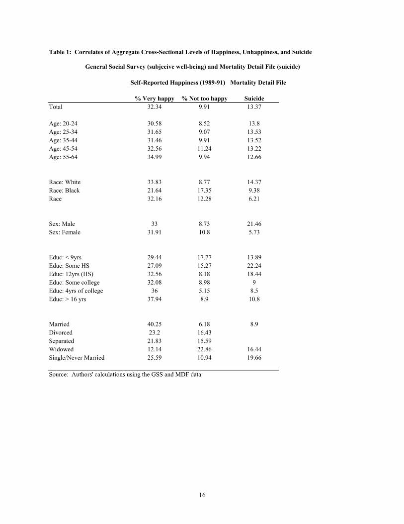
results of this analysis are reported in Table 1.

In terms of age, the results suggest a similar profile for suicide and happiness: the age-group-specific

share of respondents reporting in the highest happiness category, percent highest, rises with age, while

suicide risk falls with age. Seemingly inconsistent with the percent highest and suicide categories, the

age profile for percent lowest is not monotonically downward sloping, suggesting some asymmetry in the

low and high happiness reporting. Turning to race, whites have the highest suicide rate, followed by

blacks and then other races. The SWB data tell a very different story about race: a much larger

percentage of whites report being in the highest happiness category and a much lower fraction report

being in the lowest category than do blacks, while the percentages for other racial groups lie in between

whites and blacks. As with race, the gender pattern of suicide and SWB diverge considerably. Men are

much more likely to commit suicide than women, but the percentages reporting high and low levels of

happiness are quite similar.6

5 The downward trend in suicide may also be related to improved recognition of suicidal behavior or ailments that create suicidal feelings, improved therapeutic treatments for these conditions, and improved suicide prevention networks. 6 The difference between men and women in suicide rates may be the result of difference in means of suicide. Men are more likely to use means that have higher completion rates (jumping, guns, drowning) while woman are more likely to use means with higher probabilities of survival (overdose, cutting). In fact, attempt rates are actually two to three times higher for women than men.

7

The remainder of the table compares more behavioral or circumstantial correlates of well-being that

generally are thought to affect preferences and/or utility: marital status and educational attainment.

Being married has a consistent effect on suicide and subjective well-being, reducing suicide risk and

reported unhappiness and raising reported happiness. For the other marital statuses, the effects on suicide

and subjective well-being are less clearly aligned. For example, although being single/never married

raises suicide risk considerably relative to being separated/divorced/widowed, it has the opposite or no

effect on reported happiness and unhappiness.7 The effects of educational attainment on suicide and

SWB appear more similar. Although the relationship is far from one to one, in general, higher educational

attainment lowers suicide risk and unhappiness and increases reported happiness.

Overall, we find a weak relationship between the cross-sectional aggregate patterns in the suicide and

SWB data. The low association between these series both in the time series and across several aggregate

correlates is worrisome, and raises concern that either suicide data or SWB data, or both, may not be good

indicators of the latent variable that they are often used to measure—utility of a typical member of the

population. With this in mind, we consider how these data compare in individual level, multivariate

analyses.

IV. Micro, Multivariate Relationships Across Suicide and Subjective Well-Being Data

The lack of a strong and consistent relationship between aggregate trends and between correlates of

suicide and subjective well-being data does not necessarily imply the absence of a micro, multivariate

relationship. Aggregation bias and limited numbers of data points may be obscuring or failing to pick out

true individual-level relationships. To investigate this possibility we use individual-level data from

repeated cross-sections of the GSS and the NLMS. For the GSS, we have data from 1972-2006 and a

total of about 37,000 sample members. For the NLMS, we have data from 1978-1998 and a sample size

of about 900,000. Of these 900,000 individuals, about 63,000 died by the end of the follow-up period

(Dec. 31, 1998) and roughly 1,300 of these died of suicide. We restrict our samples from both data sets to

working-age (18 to 65 year old) individuals since much of our focus in this analysis is on variables like

labor market status and relative income that are likely to be most relevant for the preferences of the

working-age population.

7 The Mortality Detail Files data do not allow one to compute separate suicide rates for separated, divorced, and widowed.

8

Using the maximum set of variables that the GSS and NLMS have in common, we set up parallel

regressions on suicide and subjective well-being data. We then compare the results from these

regressions as a way of cross-validating the ability of suicide and SWB data to represent the underlying

latent variable on well-being. Our starting point is the familiar latent variable model in which Ui is an

unobservable index of well-being for an individual i. We model Ui as a linear function of a vector of

explanatory variables, Xi: Ui = Xi βi. The probability that Ui is below any individual-level threshold, θi

—say the threshold below which the individual would report being “not too happy” or the threshold

below which the individual would commit suicide—is then:

Prob[Ui < θi] = Prob[Xi β + θi < 0]. (1)

Our objective here is to estimate the vector β = dUi /dXi, the relative risk of Ui falling below the threshold

in question, for the thresholds of suicide, reported happiness, and reported unhappiness. We compare the

estimates from parallel regressions, using both the SWB and suicide data, arguing that a close relationship

between the results supports both the reasonableness of the data sources and the robustness of the findings

regarding determinants of utility.

For reported happiness and unhappiness, we estimate equation (1) using an ordered probit model on the

GSS data. We do ordered probit on the full 3-value scale of happiness responses rather than separate

probits for high (vs. low or medium) or low (vs. high or medium) for the sake of exposition as well as

estimation efficiency. In unreported results, we have verified that the estimated coefficients from the

separate probits look very similar to each other and to those of the ordered probit. To ease comparability

with the suicide regressions, we order the dependent variable with low at the top and high at the bottom,

so it can be thought of as a measure of unhappiness. For suicide risk, we estimate a Cox Proportional

Hazards (PH) model, given the longitudinal nature of the NLMS data.

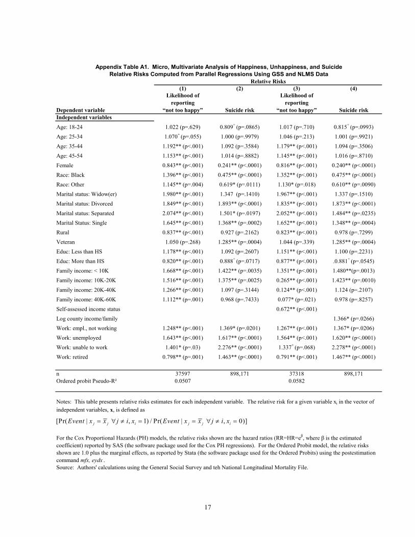
To be able to directly compare the results obtained from the GSS and NLMS, we transform the probit and

PH coefficients into their corresponding relative risk estimates. The relative risk for a given variable xi in

the vector of independent variables, Xi, is defined as

[Pr( | , 1) / Pr( | , 0)]j j i j j iEvent x x j i x Event x x j i x= ∀ ≠ = = ∀ ≠ = , where jx denotes the sample

mean. For the Cox Proportional Hazards (PH) models, the relative risks are the hazard ratios

(RR=HR=eλ, where λ is the coefficient in the PH model). For the Ordered Probit model, the relative risks

are 1.0 plus the probit marginal effects, evaluated at the sample mean.

9

The relative risk for a particular characteristic is interpreted as the probability of the event for an

individual with that characteristic relative to the probability for an individual in the omitted category. For

example, our regressions include dummy variables for whether individuals have more or less than a

secondary education, the omitted category being those who have a secondary (but not post-secondary)

education. In the regressions, we obtain a relative risk for the less than secondary education group of

1.178 in the ordered probit for unhappiness and 1.092 for the PH model of suicide. These relative risks

imply that those with less than a secondary education had a 17.8% higher risk of reporting lowest

happiness and a 9.2% higher risk of suicide compared with someone with a secondary (but not post-

secondary) education. The Xi vector in both regressions are computed similarly and include age, race,

gender, marital status, urban/rural residence, veteran status, education, employment status, family income,

and year fixed effects. The full results and p-values are reported in Appendix Table A1.

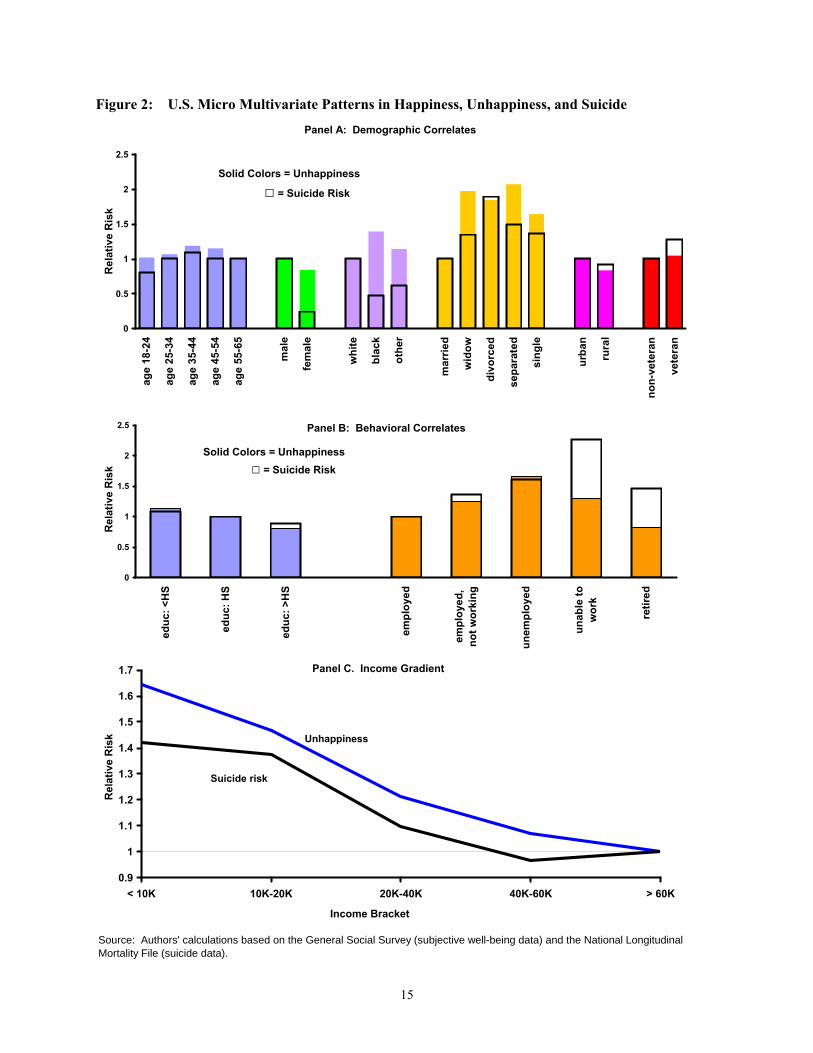
The results are summarized in Figure 2, panels A-C. Panel A shows the relative risks for the basic

demographic variables. The solid bars in the figure are the relative risks estimated from the ordered probit

regression on reported unhappiness. The black, hollow boxes show the relative risks of suicide estimated

from the Cox PH regressions. In all cases, the omitted category has a relative risk of one. Although there

are some differences in the magnitude of the coefficients in some cases, the results show strikingly similar

patterns in the effects of age, gender, marital status, urban/rural residence, and veteran status across the

two data sources. Race is the one exception, where the results move in opposite directions.

Panel B of Figure 2 shows the relative risks for educational attainment and several labor market status

variables. The educational profiles of relative risks are nearly identical, confirming the expected pattern

that unhappiness and suicide risk both fall with education. The results for the labor market status

variables also exhibit a very close association across suicide and SWB, particularly for the “employed but

not working” and unemployed categories. There is less of an association in the “unable to work” group,

but this may reflect differences in measurement of this status across data sources.8

The final comparison shown in Figure 2 is on own income. Here we plot the relative risks in terms of the

implied income gradient in each data source. Again, the pattern of the results shows a close association in

the effects of income on unhappiness and suicide risk. Both reported unhappiness and suicide risk fall

with income. Moreover, in both cases, with the exception of the first income category, the effect of

additional income declines as income grows—consistent with diminishing marginal utility of income.

8 The unable to work category is computed using a single variable in the NLMS but the combination of two variables in the GSS.

10

The last aspect of our analysis returns to the question discussed in the introduction of whether and how

relative income affects suicide risk and unhappiness (full results shown in Columns 3 and 4 of Appendix

Table A1). We add relative income to the regressions. The relative income variable for the GSS is the

respondent’s self-assessment of their own family income relative to the “typical American family,” with

possible answers of far above, above, about, below, or far below average. It should be noted that it is not

obvious what reference group the “typical American family” represents and whether this is taken to be the

national average, local area average, or something else. In the NLMS regressions, we capture relative

income by including, in addition to own family income, the average family income for their county of

residence. Note this is an abbreviated version of regressions reported in Daly, Wilson, and Johnson

(2007), which obtained very similar coefficients on variables in common.9 The GSS findings indicate

that higher perceived relative income reduces the likelihood of reporting low happiness. Similarly,

having low relative income—i.e., high county income relative to own income— increases the risk of

suicide. Consistent with previous work on relative income, both of these regressions show that relative

income is statistically significant, controlling for a wide range of demographic variables and own income.

The micro data results show a strikingly strong association between the results obtained from suicide and

SWB data. The similar pattern found in both data sources cross-validates the value of these alternative

data sources for assessing determinants of latent well-being in general and supports the findings of

diminishing marginal utility and the importance of relative income in particular.

V. Suicide and Happiness

The micro results suggest that the same factors that shift people down the happiness continuum also

increase their suicide risk. These results suggest that suicide data may be a useful way to assess the

preferences of the general population, not just those in the extreme lower tail of the distribution. To

formalize this idea, Daly, Wilson, and Johnson (2007) developed a theoretical framework describing how

one can make inferences about the preferences of the general population from the behavior of suicide

victims.

The formal model embodies the idea that suicide is an outcome of an individual’s dynamic optimization

problem weighing the present discounted value of current and expected future lifetime utility against the

value of exiting life right now. Individuals differ in their inherent levels of happiness (set points) or

9 Daly, Wilson, and Johnson 2007 performed a wide variety of robustness checks intended to rule out the possibility of spurious correlations. These checks confirmed the interpretation of the relative income findings for suicide risk.

11

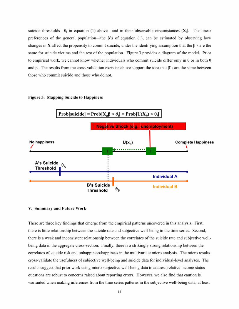
suicide thresholds—θi in equation (1) above—and in their observable circumstances (Xi). The linear

preferences of the general population—the β’s of equation (1), can be estimated by observing how

changes in X affect the propensity to commit suicide, under the identifying assumption that the β’s are the

same for suicide victims and the rest of the population. Figure 3 provides a diagram of the model. Prior

to empirical work, we cannot know whether individuals who commit suicide differ only in θ or in both θ

and β. The results from the cross-validation exercise above support the idea that β’s are the same between

those who commit suicide and those who do not.

Figure 3. Mapping Suicide to Happiness

V. Summary and Future Work

There are three key findings that emerge from the empirical patterns uncovered in this analysis. First,

there is little relationship between the suicide rate and subjective well-being in the time series. Second,

there is a weak and inconsistent relationship between the correlates of the suicide rate and subjective well-

being data in the aggregate cross-section. Finally, there is a strikingly strong relationship between the

correlates of suicide risk and unhappiness/happiness in the multivariate micro analysis. The micro results

cross-validate the usefulness of subjective well-being and suicide data for individual-level analyses. The

results suggest that prior work using micro subjective well-being data to address relative income status

questions are robust to concerns raised about reporting errors. However, we also find that caution is

warranted when making inferences from the time series patterns in the subjective well-being data, at least

No happiness

II

Negative Shock (e.g., unemployment)

II

Individual A

Individual B

A’s Suicide Threshold

B’s Suicide Threshold

θA

θB

U(xit)

Prob[suicide] = Prob[Xitβ < θi] = Prob[U(X= Prob[U(Xitit) < ) < θθii]]

Complete Happiness

12

those obtained from the GSS. Going forward, we see the results of this study as supportive of additional

and complementary work on preferences using both subjective well-being and suicide data.

13

References

Bertrand, Marianne, and Sendhil Mullainathan. "Do People Mean What They Say? Implications for

Subjective Survey Data." American Economic Review, 2001, 91(2), pp. 67-72.

Blanchflower, David G., and Andrew J. Oswald. “Well-being over time in Britain and the USA.” Journal of Public Economics, 2004, 88, no. 7-8, pp. 1359-86.

Carlsson F., Johansson-Stenman, and P. Martinsson "Do You Enjoy Having More than Others? Survey Evidence of Positional Goods" Economica, 2007, 74, 586-98. Clark, Andrew E., and Andrew J. Oswald. "Satisfaction and Comparison Income." Journal of Public

Economics, September 1996, 61(3), pp. 359-81.

Daly, M.C., Daniel Wilson, and Norman Johnson. Federal Reserve Bank of San Francisco Working Paper 2007-12.

Easterlin, Richard A. "Will Raising the Incomes of All Increase the Happiness of All?" Journal of

Economic Behavior and Organization, 1995, 27, pp. 35-48. Ferrer-i-Carbonell, Ada. “Income and well-being: an empirical analysis of the comparison income

effect.” Journal of Public Economics, June 2005, 89(5-6), pp. 997-1019. Ferrer-i-Carbonell, Ada. “Income and well-being: an empirical analysis of the comparison income

effect.” Journal of Public Economics, June 2005, 89(5-6), pp. 997-1019. Gardner,J. and Andrew J. Oswald, Money and mental wellbeing: A longitudinal study of medium-sized

lottery wins, Journal of Health EconomicsVolume 26, Issue 1, , January 2007, Pages 49-60. Luttmer, Erzo F.P. “Neighbors as Negatives: Relative Earnings and Well-Being.” Quarterly Journal of

Economics, 2005, 102(3), pp. 963-1002. McBride, M. Relative-income effects on subjective well-being in the cross-section, Journal of Economic

Behavior & OrganizationVolume 45, Issue 3, July 2001, Pages 251-278. Miller, Douglas, and Christina Paxson. "Relative Income, Race, and Mortality." Journal of Health

Economics, 2006, 25(5), pp. 979-1003. U.S. Department of Health and Human Services. National Center for Health Statistics. Mortality Detail

File, 1992 [Computer file]. Hyattsville, MD: U.S. Dept. of Health and Human Services, National Center for Health Statistics [producer], 1994. Ann Arbor, MI: Interuniversity Consortium for Political and Social Research [distributor], 1996.

Stevensen, B. and J. Wolfers. “Happiness Inequality in the United States.” Forthcoming in the Journal of

Legal Studies.

14

Figure 1: U.S. Time-Series Patterns in Happiness, Unhappiness, and Suicide

Source: Authors' calculations based on the General Social Survey (subjective well-being data) and U.S. Vital Statistics (suicide data).

Percentage of GSS Respondents in Highest and Lowest Happiness Category and the U.S. Suicide Rate

0

5

10

15

20

25

30

35

40

1972 1974 1976 1978 1982 1984 1986 1988 1990 1993 1996 2000 20040

5

10

15

20

25

30

35

40

Percent Highest Happiness

Percent Lowest Happiness

Suicide Rate

2006

Panel A Series Demeaned and Smoothed

-3

-2

-1

0

1

2

3

1972 1974 1976 1978 1982 1984 1986 1988 1990 1993 1996 2000 2004-3

-2

-1

0

1

2

3

2006

Percent Highest Happiness

Suicide Rate

Percent Lowest Happiness

15

Figure 2: U.S. Micro Multivariate Patterns in Happiness, Unhappiness, and Suicide

Source: Authors' calculations based on the General Social Survey (subjective well-being data) and the National Longitudinal Mortality File (suicide data).

0

0.5

1

1.5

2

2.5ag

e 18

-24

age

25-3

4

age

35-4

4

age

45-5

4

age

55-6

5

mal

e

fem

ale

whi

te

blac

k

othe

r

mar

ried

wid

ow

divo

rced

sepa

rate

d

sing

le

urba

n

rura

l

non-

vete

ran

vete

ran

Rel

ativ

e R

isk

Solid Colors = Unhappiness

□ = Suicide Risk

Panel A: Demographic Correlates

0

0.5

1

1.5

2

2.5

educ

: <H

S

educ

: HS

educ

: >H

S

empl

oyed

empl

oyed

,no

t wor

king

unem

ploy

ed

unab

le to

wor

k

retir

ed

Rel

ativ

e R

isk

Solid Colors = Unhappiness □ = Suicide Risk

Panel B: Behavioral Correlates

Panel C. Income Gradient

0.9

1

1.1

1.2

1.3

1.4

1.5

1.6

1.7

< 10K 10K-20K 20K-40K 40K-60K > 60K

Income Bracket

Rel

ativ

e R

isk Unhappiness

Suicide risk

16

Table 1: Correlates of Aggregate Cross-Sectional Levels of Happiness, Unhappiness, and Suicide

Mortality Detail File

% Very happy % Not too happy SuicideTotal 32.34 9.91 13.37

Age: 20-24 30.58 8.52 13.8Age: 25-34 31.65 9.07 13.53Age: 35-44 31.46 9.91 13.52Age: 45-54 32.56 11.24 13.22Age: 55-64 34.99 9.94 12.66

Race: White 33.83 8.77 14.37Race: Black 21.64 17.35 9.38Race 32.16 12.28 6.21

Sex: Male 33 8.73 21.46Sex: Female 31.91 10.8 5.73

Educ: < 9yrs 29.44 17.77 13.89Educ: Some HS 27.09 15.27 22.24Educ: 12yrs (HS) 32.56 8.18 18.44Educ: Some college 32.08 8.98 9Educ: 4yrs of college 36 5.15 8.5Educ: > 16 yrs 37.94 8.9 10.8

Married 40.25 6.18 8.9Divorced 23.2 16.43Separated 21.83 15.59Widowed 12.14 22.86 16.44Single/Never Married 25.59 10.94 19.66

Source: Authors' calculations using the GSS and MDF data.

Self-Reported Happiness (1989-91)

General Social Survey (subjecive well-being) and Mortality Detail File (suicide)

17

(1) (2) (3) (4)

Dependent variable

Likelihood of reporting

“not too happy” Suicide risk

Likelihood of reporting

“not too happy” Suicide riskIndependent variables

Age: 18-24 1.022 (p=.629) 0.809+ (p=.0865) 1.017 (p=.710) 0.815+ (p=.0993)

Age: 25-34 1.070+ (p=.055) 1.000 (p=.9979) 1.046 (p=.213) 1.001 (p=.9921)

Age: 35-44 1.192** (p<.001) 1.092 (p=.3584) 1.179** (p<.001) 1.094 (p=.3506)

Age: 45-54 1.153** (p<.001) 1.014 (p=.8882) 1.145** (p<.001) 1.016 (p=.8710)

Female 0.843** (p<.001) 0.241** (p<.0001) 0.816** (p<.001) 0.240** (p<.0001)

Race: Black 1.396** (p<.001) 0.475** (p<.0001) 1.352** (p<.001) 0.475** (p<.0001)

Race: Other 1.145** (p=.004) 0.619* (p=.0111) 1.130* (p=.018) 0.610** (p=.0090)

Marital status: Widow(er) 1.980** (p<.001) 1.347 (p=.1410) 1.967** (p<.001) 1.337 (p=.1510)

Marital status: Divorced 1.849** (p<.001) 1.893** (p<.0001) 1.835** (p<.001) 1.873** (p<.0001)

Marital status: Separated 2.074** (p<.001) 1.501* (p=.0197) 2.052** (p<.001) 1.484** (p=.0235)

Marital Status: Single 1.645** (p<.001) 1.368** (p=.0002) 1.652** (p<.001) 1.348** (p=.0004)

Rural 0.837** (p<.001) 0.927 (p=.2162) 0.823** (p<.001) 0.978 (p=.7299)

Veteran 1.050 (p=.268) 1.285** (p=.0004) 1.044 (p=.339) 1.285** (p=.0004)

Educ: Less than HS 1.178** (p<.001) 1.092 (p=.2607) 1.151** (p<.001) 1.100 (p=.2231)

Educ: More than HS 0.820** (p<.001) 0.888+ (p=.0717) 0.877** (p<.001) .0.881+ (p=.0545)

Family income: < 10K 1.668** (p<.001) 1.422** (p=.0035) 1.351** (p<.001) 1.480**(p=.0013)

Family income: 10K-20K 1.516** (p<.001) 1.375** (p=.0025) 0.265** (p<.001) 1.423** (p=.0010)

Family income: 20K-40K 1.266** (p<.001) 1.097 (p=.3144) 0.124** (p<.001) 1.124 (p=.2107)

Family income: 40K-60K 1.112** (p=.001) 0.968 (p=.7433) 0.077* (p=.021) 0.978 (p=.8257)

Self-assessed income status 0.672** (p<.001)

Log county income/family 1.366* (p=.0266)

Work: empl., not working 1.248** (p<.001) 1.369* (p=.0201) 1.267** (p<.001) 1.367* (p=.0206)

Work: unemployed 1.643** (p<.001) 1.617** (p<.0001) 1.564** (p<.001) 1.620** (p<.0001)

Work: unable to work 1.401* (p=.03) 2.276** (p<.0001) 1.337+ (p=.068) 2.278** (p<.0001)

Work: retired 0.798** (p=.001) 1.463** (p<.0001) 0.791** (p<.001) 1.467** (p<.0001)

n 37597 898,171 37318 898,171Ordered probit Pseudo-R² 0.0507 0.0582

Source: Authors' calculations using the General Social Survey and teh National Longitudinal Mortality File.

Notes: This table presents relative risks estimates for each independent variable. The relative risk for a given variable xi in the vector of independent variables, x, is defined as

For the Cox Proportional Hazards (PH) models, the relative risks shown are the hazard ratios (RR=HR=eβ, where β is the estimated coefficient) reported by SAS (the software package used for the Cox PH regressions). For the Ordered Probit model, the relative risks shown are 1.0 plus the marginal effects, as reported by Stata (the software package used for the Ordered Probits) using the postestimation command mfx, eydx .

Relative Risks

Appendix Table A1. Micro, Multivariate Analysis of Happiness, Unhappiness, and SuicideRelative Risks Computed from Parallel Regressions Using GSS and NLMS Data

[Pr( | , 1) / Pr( | , 0)]j j i j j iEvent x x j i x Event x x j i x= ∀ ≠ = = ∀ ≠ =