PNNL-16099

Hanford Soil Inventory Model (SIM) Rev. 1 User’s Guide B. C. Simpson R. A. Corbin M. J. Anderson C. T. Kincaid September 2006 Prepared for the U.S. Department of Energy under Contract DE-AC05-76RL01830

DISCLAIMER This report was prepared as an account of work sponsored by an agency of the United States Government. Neither the United States Government nor any agency thereof, nor Battelle Memorial Institute, nor any of their employees, makes any warranty, express or implied, or assumes any legal liability or responsibility for the accuracy, completeness, or usefulness of any information, apparatus, product, or process disclosed, or represents that its use would not infringe privately owned rights. Reference herein to any specific commercial product, process, or service by trade name, trademark, manufacturer, or otherwise does not necessarily constitute or imply its endorsement, recommendation, or favoring by the United States Government or any agency thereof, or Battelle Memorial Institute. The views and opinions of authors expressed herein do not necessarily state or reflect those of the United States Government or any agency thereof.

PACIFIC NORTHWEST NATIONAL LABORATORY operated by BATTELLE

for the UNITED STATES DEPARTMENT OF ENERGY

under Contract DE-AC05-76RL01830

Printed in the United States of America

Available to DOE and DOE contractors from the Office of Scientific and Technical Information,

P.O. Box 62, Oak Ridge, TN 37831-0062; ph: (865) 576-8401 fax: (865) 576-5728

email: reports@adonis.osti.gov

Available to the public from the National Technical Information Service, U.S. Department of Commerce, 5285 Port Royal Rd., Springfield, VA 22161

ph: (800) 553-6847 fax: (703) 605-6900

email: orders@ntis.fedworld.gov online ordering: http://www.ntis.gov/ordering.htm

This document was printed on recycled paper.

PNNL-16099

Hanford Soil Inventory Model (SIM) Rev. 1 User’s Guide NuvotecUSA, Inc. B. C. Simpson R. A. Corbin M. J. Anderson Pacific Northwest National Laboratory C. T. Kincaid September 2006 Prepared for the U.S. Department of Energy under Contract DE-AC05-76RL01830 Pacific Northwest National Laboratory Richland, Washington 99352

iii

Summary

The objective of this document is to support the simulation results reported by Corbin et al. (2005) by providing a user’s guide for Hanford Soil Inventory Model (SIM) Rev. 1. This document is meant to provide technical support of Corbin et al. (2005), which is a significant revision and update to an earlier product Simpson et al. (2001). The SIM application computed waste discharges composed of 75 analytes at 377 waste sites (liquid disposal, unplanned releases, and tank farm leaks) over an operational period of approximately 50 years. The development and application of SIM was an effort to develop a probabilistic approach to estimate comprehensive, mass balanced-based contaminant inventories for the Hanford Site post-closure setting. A computer model capable of calculating inventories and the associated uncer-tainties as a function of time was identified to address the needs of the Remediation and Closure Science (RCS) Project. This user’s guide is a companion document to a report on the requirements, conceptual model, simulation, methodology, testing, and quality assurance associated with the Hanford SIM Rev. 1 (Simpson et al. 2006)

To estimate mass balanced contaminant inventories and their uncertainties for the Hanford Site post-closure setting, a stochastic simulation method (a Monte Carlo-type calculation) was selected to provide estimates of inventory and uncertainty. The Open Crystal Ball (OCB) statistical package was selected in 2002 for application in this model.

The design of SIM is highly modular with separate data input (Microsoft Excel) and calculation engine (OCB.dll) files administered through an interface application that acquires the inputs, manages the data reporting, and creates the output files. Each data input is considered an independent variable; therefore, the waste stream composition/properties and waste stream discharge histories for the waste disposal sites can be examined and developed using a variety of source data (e.g., historical process data, tank waste modeling, etc.) and assumptions without impacting other variables.

There are several limitations to the application of SIM. Principal among them is that history match-ing the model results with reference data was not a goal of SIM prior to publication of model results (e.g., Corbin et al. 2005); rather, history matching is an ongoing effort that relies on the interpretation of field characterization data. Other limitations of the software are associated with the reliability and availability of input data, because the inputs used to generate the inventories using the SIM architecture are controlled by various independent organizations (Pacific Northwest National Laboratory; CH2M HILL Hanford Group, Inc.; and/or Fluor Hanford, Inc.), and because of the stability/appropriateness of the various physical and chemical assumptions used in quantifying model behavior. While an intensive history matching effort has not been undertaken, some limited comparisons between model results and historical data were performed. Accordingly, despite its limitations, the SIM results reported by Corbin et al. (2005) are the best available information on contaminant releases to the waste sites simulated.

A programmatic limitation of this effort is as a consequence of the software business environment there has been refinement and updating of OCB and Crystal Ball (CB), thus the SIM platform developed as part of the RCS Project and documented in Corbin et al. (2005) is not currently available software. There remains capability to do inventory calculations with this model with the current resources, licenses, and support from Decisioneering, however, acquiring additional licenses for the legacy version of OCB and CB in use in order to distribute the software is not possible.

v

Terms/Acronyms AMD advanced micro devices CB Crystal Ball DVD digital video disc GB gigabytes GHz gigahertz HDW Hanford Defined Waste (Model) OCB Open Crystal Ball LHS Latin hypercube sampling MB megabytes ML megaliters PNNL Pacific Northwest National Laboratory RAM random access memory RCS Remediation and Closure Science (Project) SIM Soil Inventory Model UPR unplanned release UPS uninterruptible power supplies USB universal serial bus

vii

Contents Executive Summary ............................................................................................................................ iii Terms/Acronyms................................................................................................................................. v 1.0 Project Requirements and Overview .......................................................................................... 1.1 1.1 Program Development........................................................................................................ 1.1 1.2 Overview of Software Capabilities .................................................................................... 1.1 1.3 Hardware and Software Requirements............................................................................... 1.2 1.3.1 Software System Requirements............................................................................... 1.3 1.4 Program Documentation .................................................................................................... 1.3 2.0 Modeling Environment............................................................................................................... 2.1 2.1 Simulation Control ............................................................................................................. 2.1 2.1.1 Setup Worksheet...................................................................................................... 2.1 2.1.2 Legend Worksheet................................................................................................... 2.3 2.2 Input File Preparation, Variable Definition and Parameterization ..................................... 2.8 3.0 Input Modification through the MS Excel User Interface .......................................................... 3.1 3.1 Adding or Editing a Site for Inclusion in the Simulation................................................... 3.1 3.2 Adding or Editing Site Volumes ........................................................................................ 3.1 3.3 Adding or Editing a Waste Stream Entry........................................................................... 3.2 3.4 Defining Analyte Concentrations in a Waste Stream......................................................... 3.3 3.5 Editing Analytes to SIM..................................................................................................... 3.4 3.6 Adding a Waste Stream Density Definition ....................................................................... 3.5 3.7 Determining Correction Factor Values .............................................................................. 3.5 4.0 Executing a Soil Inventory Model Simulation ........................................................................... 4.1 4.1 Distributed Computing....................................................................................................... 4.2 4.1.1 Splitting Runs.......................................................................................................... 4.2 4.1.2 Merging the Runs .................................................................................................... 4.3 5.0 Quality Assurance and Error Recovery Guidance...................................................................... 5.1 5.1 Convergence....................................................................................................................... 5.1 5.2 Top 10 Lists........................................................................................................................ 5.2 5.3 Blackbox Test..................................................................................................................... 5.2 5.4 Volume Balance Macro...................................................................................................... 5.3 5.5 Other QA and Error Recovery Tests .................................................................................. 5.4 6.0 SIM Outputs ............................................................................................................................... 6.1 6.1 Category (Operable unit) Workbook Results..................................................................... 6.1 6.2 SAC Output Files ............................................................................................................... 6.1

viii

6.3 Summary Inventory Spreadsheets ...................................................................................... 6.2 6.4 Top 10 Lists Spreadsheets.................................................................................................. 6.2 7.0 References .................................................................................................................................. 7.1

Figures 2.1 Simulation Control—Setup Worksheet Illustration.................................................................... 2.2 2.2 Legend Identification Matrices—Locations, Analytes, Waste Streams ..................................... 2.4 2.3 Legend Worksheet (continued)—Distributed Computing Administration................................. 2.5 2.4 SIM Dialog Box ......................................................................................................................... 2.7

Tables 1.1 Hardware Requirements for SIM Operation............................................................................... 1.2 2.1 Available Distribution Parameter Definitions ............................................................................ 2.8 2.2 Proposed Distribution Selection Criteria and Application ......................................................... 2.9 3.1 SiteInput Worksheet Example .................................................................................................... 3.2 3.2 AnalyteInput Worksheet Example .............................................................................................. 3.4 3.3 DensityInput Worksheet Example .............................................................................................. 3.5 3.4 CorrFactors worksheet Example ............................................................................................... 3.6

1.1

1.0 Project Requirements and Overview

The focus of the development and application of a soil inventory model as part of the Remediation and Closure Science (RCS) Project managed by Pacific Northwest National Laboratory (PNNL) was to develop a probabilistic approach to estimate comprehensive, mass balanced-based contaminant inventories for the Hanford Site post-closure setting. The outcome of this effort was the Hanford Soil Inventory Model (SIM). This document is a user’s guide for the Hanford SIM.

The principal project requirement for SIM was to provide comprehensive quantitative estimates of contaminant inventory and its uncertainty for the various liquid waste sites, unplanned releases, and past tank farm leaks as a function of time and location at Hanford. The majority, but not all of these waste sites are in the 200 Areas of Hanford where chemical processing of spent fuel occurred. A computer model capable of performing these calculations and providing satisfactory quantitative output representing a robust description of contaminant inventory and uncertainty for use in other subsequent models was determined to be satisfactory to address the needs of the RCS Project. The ability to use familiar, commercially available software on high-performance personal computers for data input, modeling, and analysis, rather than custom software on a workstation or mainframe computer for modeling, was desired.

1.1 Program Development

The objective of the RCS Project is to provide new knowledge, data, tools, and the understanding needed to make sound remediation decisions. The RCS Project is focused on resolving key technical issues that help inform and influence remediation decisions and decisions that impact the closure of the Hanford Site. This effort is being done in collaboration with the Groundwater Remediation Project managed by Fluor Hanford, Inc.; the Tank Farm Vadose Zone Project managed by CH2M HILL Hanford Group, Inc.; and the Hanford Remediation Assessments and Characterization of Systems Project managed by PNNL. Because the Hanford SIM has matured into an application tool, this task and other ongoing efforts are funded under the Characterization of Systems Project.

The inventory effort with regard to vadose zone and groundwater contamination is focused on extending the Hanford Defined Waste (HDW) Model (Agnew et al. 1997; Higley et al. 2004) and other process knowledge to quantify contaminant inventories and uncertainties for liquid waste disposal sites, unplanned releases, and tank leaks that directly received process waste in the 200 Areas of the Hanford Site; and a select number of sites in the 300 Area. The software described here is an improved version of the initial Hanford SIM published in 2001 (Simpson et al. 2001). The current software has been used to estimate the inventories discharged or leaked to the vadose zone (Corbin et al. 2005).

1.2 Overview of Software Capabilities

The current Hanford SIM application simulates the discharge of 75 analytes at 377 waste sites over an operational period of approximately 50 years. SIM provides annual and consolidated inventory and uncertainty estimates for each analyte and waste site, with the capability to group waste site contaminant inventories in a variety of ways. The Monte Carlo calculations can be done in either simple random sampling or Latin hypercube sampling (LHS) (Iman and Conover 1982)with large numbers of iterations.

1.2

The SIM architecture is flexible enough to add/modify waste streams and waste sites as needed or focus the model calculations and analyses on a specific set of years, waste sites, and analytes. Additional post-processing quality assurance, diagnostic, and analytical tools exist as part of the overall system to further evaluate the SIM results.

1.3 Hardware and Software Requirements

Using conventional personal computers for this task was desired; thus, there are several hardware-based challenges that impede the execution of the model. These challenges are associated with reading and writing the input data, performing large numbers of computations, and managing the output data. Thus, operation of SIM is predominantly limited by the amount of available random access memory (RAM) provided in the computer. However, because the Windows XP operating system constrains RAM memory use to 1.3 Gigabytes (GB), more RAM above this limit does not enhance performance. Table 1.1 details the minimum and recommended hardware necessary to operate SIM.

Computers meeting the minimum requirements can be used to run SIM, but the run times for the simulations become exceedingly long. A complete converged model run (assuming a typical 2005 model configuration) using the recommended hardware configuration distributed over four computers takes over 100 hours of chronological time or over 400 machine-hours of computing time. Therefore, using a single machine with the minimum requirements to execute a full simulation as defined would take in excess of two weeks of continuous operation to complete.

Table 1.1. Hardware Requirements for SIM Operation

Minimum Required Hardware to Operate/Execute SIM Recommended Hardware to Operate/Execute SIM

Intel Pentium 4 system, with a clock speed of at least 2.53 GHz (SIM has not been tested on the AMD platform)

Several Intel-based Pentium 4 systems with clock speeds greater than 3.0 GHz

1 GB of RAM 2 GB of RAM 1 GB of free hard drive space 5 GB of free hard drive space Smaller than a 20” monitor Greater than a 20” monitor

PC Case with room for and at least operating 4 case fans

PC Case operating with the original equipment manufacturer’s installed fan

Uninterruptible power supplies (UPS) DVD-RW DVD-R USB mass storage drive

AMD = Advanced micro devices. DVD = Digital video disc. GB = Gigabytes. GHz = Gigahertz. PC = Personal computer. RAM = Random access memory. SIM = Soil Inventory Model. UPS = Uninterruptible power supplies. USB = Universal storage bus.

1.3

The amount of time necessary to complete a simulation varies as a function of the number of trials, sites, and analytes being evaluated, but other than for relatively simple troubleshooting situations, these models are very demanding with regard to the amount of time they take to perform.

1.3.1 Software System Requirements

These are the minimum software requirements for performing calculations using the current SIM and its associated infrastructure:

• Windows XP Professional;1 provides the operating system for the computer

• Windows.NET 1.11 provides the application environment

• Crystal Ball2 v5.2provides the ability to evaluate scenarios using macros as part of the quality assurance infrastructure

• Open Crystal Ball2 (OCB.dll); provides the computational engine to perform the stochastic calculations

• C# interface (OCBHanford3); administers the simulation by managing inputs and outputs through OCB

• Microsoft Excel1 2000 (or later); user interface for data input/output and analysis.

A complete discussion of Hanford SIM requirements, design, and limitations can be found in Simpson et al. (2006).

1.4 Program Documentation

The proof-of-principle software product and its application were documented in Simpson et al. (2001). That product, SIM Rev. 0, was applied to generate inventory estimates for 46 radionuclides and 27 chemicals from 88 liquid waste disposal sites. These estimates provided uncertainty bounds around the calculated inventory using uncertainties defined in the input data.

The successful outcome of the proof-of-principle task led to the development of the effort described in Corbin et al. (2005). In addition to the soil waste site inventories, the RCS Project also coordinated with tasks funded by the Tank Farm Vadose Zone Project for particular unplanned releases (i.e., past tank leak losses) documented for boiling waste tanks (S, SX, A, and AX), dilute waste tanks (B, BX, T, TY, and C), and concentrated tank leaks (BY, U, and TX) (Field and Jones 2005). The scope of activities for fiscal years 2002 through 2005 was to provide comprehensive chemical and radionuclide inventories and uncertainties for a variety of liquid waste disposal sites, unplanned releases, and tank leaks as a function

1 Software product of Microsoft Corporation, Redmond, Washington. 2 Software product of Decisioneering, Denver, Colorado. 3 OCBHanford is part of the Hanford SIM model and not a vendor product.

1.4

of time using SIM, Rev. 1. These estimates present a statistical description of the inventories for these sites and, thus, consist of a mean, median, standard deviation about the mean, and several percentiles for each analyte for each year of operation.

There are several substantial differences between SIM Rev. 0 and SIM Rev. 1. Because SIM Rev. 0 was a proof-of-principle effort (Simpson et al. 2001), the model was modest in scope and relatively straightforward. The initial SIM used a combination of HDW Model Rev. 4 (Agnew et al. 1997) and historical data regarding analytes, waste streams, and a limited number of significantly simplified assumptions. Only 16 waste streams were used to describe the waste stream inputs to the disposal sites. The uncertainty distributions selected to represent the waste stream conditions were highly constrained (normal, lognormal, or triangular), often based on limited data, and not unusually large in magnitude.

The current model, SIM Rev. 1, is based on the more recent HDW Model Rev. 5 (Higley et al. 2004) as well as the latest ORIGEN2 simulation of production estimates (Watrous et al. 2002). More sophisti-cated technical assumptions and capabilities were incorporated as part of SIM Rev. 1. It includes the chemical and radionuclide composition estimates of 196 waste streams for computing inventories for 377 waste sites.

2.1

2.0 Modeling Environment

There are three principal elements to the SIM system: the SIMInput_Base workbook, OCBHanford, and the OCB.dll. The SIMInput_Base data file is a MS Excel workbook that contains the necessary input definitions. The OCBHanford C# interface code extracts the necessary information from the various SIMInput_Base worksheets to allow the OCB.dll to perform calculations as needed and is accessed through activating a dialog box. The OCBHanford C# interface code also creates the output spread-sheets, writes the results to the output files, and writes summary results into the SIMInput_Base file. The OCB.dll performs all the stochastic calculations and does not have a direct user interaction.

2.1 Simulation Control

The SIMInput_Base workbook has two worksheets related to simulation control—the Setup work-sheet and the Legend worksheet; these worksheets provide an interface for the user to define the bound-aries and reporting requirements of the simulation. It is the primary interface with which the end user will interact.

The other interface element that controls SIM is OCBHanford. It is accessed using a desktop shortcut and operated via a dialog box which activates the simulation. Once the parameters in the SIMInput_Base file are set, the specific file to be used must be opened using OCBHanford and the program will execute. The calculation will then proceed as directed and outputs are generated until the simulation is completed or interrupted.

2.1.1 Setup Worksheet

This is the top level administrative spreadsheet. An illustration of the Setup worksheet is provided in Figure 2.1. The Setup spreadsheet is used to define, control, and report the Monte Carlo calculation parameters of SIM:

• Seed (Cell B4). This parameter is the random number seed. As part of the OCB kernel, if a seed value greater than zero is entered into this cell, the results will be exactly repeatable because a common random number list will be used. If the seed is zero, the random number generator will provide a similar result to a given model such that, with enough trials, the values will converge to whatever tolerance is desired, but the results will not be exactly repeatable.

• Trials (Cell B5). This is the number of times the model is simulated with random values for assumptions within the distribution definition.

• Sampling Method (Cell B6). Open Crystal Ball has two methods of simulation, Monte Carlo and LHS. By setting this value to 0, a Monte Carlo calculation using a simple random sampling method will be performed.

2.2

Figure 2.1. Simulation Control—Setup Worksheet Illustration

In setting this value to 1, the LHS method will be selected. This sampling method works by segmenting the assumption's probability distribution into a number of non-overlapping intervals, each having equal probability.

• LHS Sample Size (Cell B8). For the LHS method, this value controls the number of interval segments and sample points across the segmented distribution for an assumption. The outcome of dividing the sample size value by the number of trials must result in an integer, otherwise the model will not execute.

• Start/End/Duration (Cells B13…B15). This is the duration of the simulation. A calculated duration for the simulation using these start and end times is used, rather than the dynamic values reported in the Application Window. This value is not a running total; thus, the total time will not be calculated unless the simulation completes.

2.3

• Create SAC Output (Cells A17…A20). The button, Create SAC Output activates a command that generates an output file that the SAC model can read and use in its computations (Kincaid et al. 2006). This output file is different in structure from the direct output files generated by SIM and does not contain the summary statistics for a site or operable unit, but contains the same site-year-analyte inventory and aggregate concentration and volume data.

• Percentiles (Cells G3…G23). There are twenty-one percentiles in a list. The number of percentiles reported must remain at twenty-one and are user defined. Percentiles are required for reporting the output to the SumFrcLiquid, SumFrcSolid, and SumFrcTotal worksheets in the SIMInput_Base file. The percentiles may have varying intervals, but must be non-duplicate values from 0 through 100.

• Save Results Directory (Cell B26). This cell sets the pathname for saving the output from SIM.

• Notification (Cells B27, C27, and D27). These cells provide an e-mail address with subject line that can be notified as the simulation progresses, should a simulation require a long time to execute (e.g., greater than a workday) and the user desires a means of monitoring the progression of the simulation remotely.

• Optimization Parameters: Trials per loop (Cell B31). This cell defines the calculation size performed in one pass through the simulation. It must evenly divide into the number of trials and can be no greater than the number of trials.

• Combine Top 10 Lists (Cell B35). This cell defines the pathway for recombining distributed models and creating a consolidated Top 10 list. Cells G34 to H36 define a button, Merge Top 10 Lists, for executing the command to initiate reconstitution of the distributed Top 10 lists into a single file.

• List the Resulting SimInput files (full location) to Merge into ‘THIS’ Empty Directory (Cells B39…B48). This merging macro (Merge Summaries) uses the listed SIMInput_Base files to determine which set of distributed results are to be merged into the newly specified directory. A set of successful simulations are assumed to have occurred and that the various output files are located in the pathways specified with the above listed SIMInput_Base files.

2.1.2 Legend Worksheet

This worksheet is the backbone of the simulation. It defines the boundaries of the simulation, i.e., which disposal sites, waste streams, and analytes that are to be included in calculating inventories in a simulation; it also controls the distributed computing features in SIM.

Figures 2.2 and 2.3 provide an example of the Legend worksheet. All input information is sorted and configured as defined in the Legend sheet. All of the data input sheets are directly related to the Legend. The SiteInput spreadsheet provides specific disposal volume data, describing the waste site, year(s) of operation, and the waste stream(s) for both liquid and solids. The AnalyteInput spreadsheet defines the waste stream concentration data. DensityInput defines the density of a waste stream phase (solid or liquid).

2.4

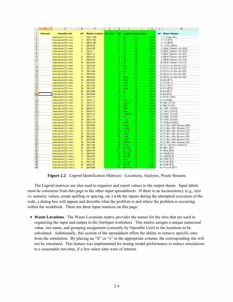
Figure 2.2. Legend Identification Matrices—Locations, Analytes, Waste Streams

The Legend matrices are also used to organize and report values to the output sheets. Input labels must be consistent from this page to the other input spreadsheets. If there is an inconsistency (e.g., text vs. numeric values, errant spelling or spacing, etc.) with the inputs during the attempted execution of the code, a dialog box will appear and describe what the problem is and where the problem is occurring within the workbook. There are three input matrices on this page:

• Waste Locations. The Waste Locations matrix provides the names for the sites that are used in organizing the input and output in the SiteInput worksheet. This matrix assigns a unique numerical value, site name, and grouping assignment (currently by Operable Unit) to the locations to be calculated. Additionally, this section of the spreadsheet offers the ability to remove specific sites from the simulation. By placing an “X” or “x” in the appropriate column, the corresponding site will not be simulated. This feature was implemented for testing model performance to reduce simulations to a reasonable run-time, if a few select sites were of interest.

2.5

Figure 2.3. Legend Worksheet (continued)—Distributed Computing Administration

• Analytes/Radionuclides. The Analytes/Radionuclides matrix identifies the chemical species/ isotopes being inventoried for the sites and assigns a unique numerical index value, appropriate element/chemical name, and corresponding units in SIM. The unit assignments for each analyte/ radionuclide are directly copied from these values to the output. Additionally, this section of the spreadsheet offers the ability to remove specific analytes from the simulation. By placing an “X” or “x” in the appropriate column, the corresponding analyte will be removed. This feature was imple-mented for testing model performance to reduce simulations to a reasonable run-time, if a few select analytes were of interest.

• Waste Stream. This matrix assigns a unique numerical index value and name to each waste stream used in the AnalyteInput worksheet.

The waste location and waste stream matrices are not currently fixed in size in the modeling code, but the number of analytes/radionuclides that can be present in a waste stream is fixed at 75 (e.g., the current set of code instructions describes the analytes in a waste stream as a fixed array). If there is a need to add locations or waste streams to the model, they can be added to the current matrix, and included in SIM by maintaining the appropriate identification index number sequence and labeling. Analytes can also be

2.6

modified within a waste stream so long as they are consistent in labeling and indexing throughout the SIM definition worksheets (e.g., Legend and AnalyteInput). Similarly, if a parameter needs to be deleted, that change can be accommodated as well; there is the option of excluding analytes from the calculation as a feature or setting the concentration values to zero in the waste stream definition, but there must be 75 specific elements described in the array.

However, there cannot be any blank cells in the input matrices because the modeling code determines the maximum number of sites, analytes, and waste streams in each matrix by stepping through the array until it finds an undefined cell. Thus, the elements of these matrices must be contiguous and the identi-fication index numbers must be sequential integers for the model code to execute. Cells containing a space, ‘ ‘, within a label are not considered “undefined” cells, but may interrupt the model execution because of the potential ambiguity. If this error occurs, the model will describe the problem and its location to the user within the workbook in a message box.

Because of the size and run times associated with SIM, a simple distributed computing function was incorporated. The distributed computing management function was placed in the Legend worksheet of the production workbook. By placing an "X" or "x" in the appropriate column then executing the macro OpUnit_Selection, the corresponding sites of that Operable Unit are removed from the simulation. By using the Update Operable Unit List and Split into Sections macro command, the computer automati-cally loads a file that is reasonably balanced as a function of the number of machines used to perform a simulation with the pieces having approximately concurrent run-time completions.

These pieces are estimated using the number of site-year elements as a metric and are split into roughly equal numbers; however, sites within a specified operable unit are conserved (i.e., all members of an operable unit grouping are maintained together) within the same sub-file. A simulation can be split among as many machines as is needed; however, the reconstitution function (Merge in the Setup worksheet) can handle a maximum of 10 files at a time.

On activation of OCBHanford, a dialog box appears (Figure 2.4). OCBHanford is the executable file containing the C# code that manages the communication between the input file and the calculation engine, provides the data reporting, and creates the output files. The OCBHanford dialog box also presents a series of diagnostic data regarding simulation time and computing resources demand that can be useful in gauging model parameter settings. The dialog box has only one drop-down menu command, which is “File,” and from there the file to be used must be selected. The SIMInput_Base file can then be checked for inconsistencies or errors by checking the appropriate box, and selecting “Test Distributions.” The code will then review the various input definitions and assign the index identification numbers used to organize the inputs and calculate the results. If there is an error or problem with the SIMInput_Base file, a series of message boxes will appear describing them and their location within the workbook.

2.7

Figure 2.4. SIM Dialog Box

2.8

During initialization of the model, several actions occur. The site labels in the SiteInput spreadsheet are matched to the site labels in the Legend spreadsheet and indexed to their specific site identification numbers from the Legend spreadsheet. These indices are assigned to the first column of the SiteInput sheet and are used by the OCB interface to execute and administer the calculation. Similarly, the waste stream labels in the SiteInput spreadsheet are matched to the waste streams in the Legend spreadsheet and indexed to their specific waste stream identification number from the Legend spreadsheet and assigned the waste stream identification numbers to the second column of the SiteInput sheet.

Once the model is initialized, if the file is satisfactory, unchecking the box and selecting “Calculate” will activate SIM and calculation will commence. If during a simulation a problem is discovered or if the user has a need, there are “Pause” and “Cancel” commands that will alternately temporarily suspend the simulation or stop and quit the application entirely as desired.

2.2 Input File Preparation, Variable Definition and Parameterization

Each model input (total volume, volume percent solids, liquid composition, solids composition, liquid density, solids density, unit correction factors, and simulation administration boundaries) must have a practical, defensible, quantitatively defined set of values. These inputs will characterize the typical value and range of uncertainty for each variable in the calculation or govern the execution of the simulation. Distributions for modeling parameters and their quantitative descriptions can be assigned by a variety of methods.

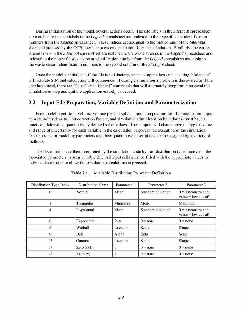
The distributions are then interpreted by the simulation code by the “distribution type” index and the associated parameters as seen in Table 2.1. All input cells must be filled with the appropriate values to define a distribution to allow the simulation calculations to proceed.

Table 2.1. Available Distribution Parameter Definitions

Distribution Type Index Distribution Name Parameter 1 Parameter 2 Parameter 3

0 Normal Mean Standard deviation 0 = unconstrained; value = low cut-off

1 Triangular Minimum Mode Maximum

4 Lognormal Mean Standard deviation 0 = unconstrained; value = low cut-off

6 Exponential Rate 0 = none 0 = none

8 Weibull Location Scale Shape

9 Beta Alpha Beta Scale

12 Gamma Location Scale Shape

17 Zero (null) 0 0 = none 0 = none

18 1 (unity) 1 0 = none 0 = none

2.9

Table 2.2 describes commonly selected reasons for assigning distributions and how they are currently applied in SIM. Further guidance on the development of parameter definitions and conventions currently used in SIM can be found in Corbin et al. (2005); however the requirements and methods to complete a satisfactory set of input files to execute a simulation are not necessarily tied to these assumptions.

Table 2.2. Proposed Distribution Selection Criteria and Application

Distribution Reasons for Using Distribution Where/How Used in Hanford

SIM

Normal Conventional statistical selection when variable uncertainty behavior is unknown or sparsely quantified

Tank leak volumes; volume percent solids

Triangular Conventional engineering selection when variable uncertainty behavior is sparsely quantified but a typical range is indicated

Liquid waste disposal volumes; selected chemical concentrations

Lognormal Variable uncertainty behavior is considered to be strictly positive, having a strong central tendency and long tail

Chemical concentrations; densities; selected UPR volumes

Exponential Variable uncertainty behavior is considered to be strictly positive, having a strong first impulse with decay behavior

Selected UPR volumes

Weibull Optional variable uncertainty behavior Not currently used in SIM

Beta Variable behavior is conditioned to poorly fit data in order to minimize bias and provide strictly non-negative results

Radionuclide concentrations

Gamma Optional variable uncertainty behavior Not currently used in SIM

Zero (null) Reasonable certainty regarding the absence of a particular quantity; also used in software testing

Volume (all), concentration (all)

1 (unity) Used as part of software calculation testing Not currently used in SIM

SIM = Soil Inventory Model. UPR = Unplanned release.

3.1

3.0 Input Modification through the MS Excel User Interface

As previously noted, a series of MS Excel worksheets (SiteInput, AnalyteInput, DensityInput, CorrFactors, Legend, and Setup) were created in a workbook as a user interface and integrated into a comprehensive model input data file. The following sections describe the steps necessary to make changes or additions to the variable definitions.

3.1 Adding or Editing a Site for Inclusion in the Simulation

1. Select the Legend sheet from the SIMInput_Base file (refer to Figure 2.2).

2. Examine the list that extends from column F cell 2 (F2) down to see if the site to be added already exists in the model.

3. At the bottom of the list started in cell F2 (or in F2 if it is blank and a new series of sites is being simulated), enter in the name of the site. There cannot be any blank spots in the list (e.g., the list must be continuous and sequential) and the site label must be unique.

4. In Column E, next to the name of the newly entered site, enter in the next consecutive number. The number in column E should be the row the site was added into minus 1. If the site was added into cell F527, the index value in E527 should be 526.

5. On the same row, in column D, enter in the name of the operable unit (e.g., category) to which the site belongs. If this is an operable unit name that has been used before, it is recommended that the label be copied and pasted into this cell to ensure that the name is identical.

6. If a site label needs to be edited, the name can be edited in the Legend sheet and the prior label be replaced in the SiteInput worksheet as a correction.

3.2 Adding or Editing Site Volumes

Quantifying and parameterizing the waste volume for a site involves a significant degree of analysis and judgment, the details of which are outside the scope of this user’s guide. However, as a brief over-view of this process, the initial step in this phase is identifying and verifying source information and assumptions regarding the site’s overall volume, individual volume contributions, and its operating life (e.g., annual waste receipts).

This information must then be entered into the SiteInput worksheet in the appropriate cells, must be in a form that can be used by the program (e.g. properly assigning and quantifying the distributions), and does not violate any of the various physical, chemical, or mathematical boundary conditions inherent in the simulation (e.g., waste volumes are greater than or equal to zero, waste streams are charge balanced systems, lognormal distributions are strictly positive, etc.). The indices in the Legend #, s (Legend worksheet site index number) and Legend #, w (Legend worksheet waste stream index number) are assigned as part of simulation initialization and are not part of the data entry in the SiteInput worksheet.

3.2

The default total volume unit basis is megaliters (e.g., in the SiteInput file, a value of 1 = 1,000,000 L); the volume percent solids basis is percent, expressed as a decimal (e.g., in the SiteInput, a value of 0.01 = 1%). As illustrated in Table 3.1, the data entry process for the SiteInput worksheet follows:

1. From the SIMInput_Base file, select the SiteInput sheet.

2. Enter the site label, corresponding to the site name in the Legend worksheet.

3. Enter the site year of operation for that waste site-waste stream-year combination (from 1944 to 2001).

4. Enter the site waste stream label, corresponding to the site name in the Legend worksheet.

5. Enter the distribution type for the waste volume.

6. Enter the parameterization for total volume for that waste site-waste stream-year combination.

7. Enter the parameterization for volume percent solids for that waste site-waste stream-year combination.

8. Once entered, the quantitative description can be modified as needed.

9. If revisions to the input definition are necessary as a result of newly discovered site information (or other technical/programmatic reasons), maintaining a change control log is recommended to provide traceability and defensibility of the change.

Table 3.1. SiteInput Worksheet Example

Legend #

Legend # Total Volume (ML) Vol % Solids

s w Site Year Waste Stream Dist Type Parm 1 Parm 2 Parm 3

Dist Type

Parm 1

Parm 2

Parm 3

1 45 200-E-100 1945 BiPO4 (BT1) Cool Wtr-Stm Cond

1 0.00219 0.00438 0.00657 17 0 0 0

65 50 216-A-19 1955 PUREX (P1) Cold Start

1 0.825 1.10 1.38 1 0.045 0.09 0.125

3.3 Adding or Editing a Waste Stream Entry

There can be as many waste streams as is required (within certain practical limits) to perform a simulation in SIM. The label identifying the waste stream must be defined in the Legend worksheet and is assigned by the analyst when defining the site in the SiteInput worksheet. The waste stream must also be assigned a unique and appropriately descriptive label. Although SIM does not use the location label per se as part of the calculation, a well selected waste stream label assists in troubleshooting, analysis, and

3.3

evaluation of the simulation inputs and outputs as well as providing traceability to reference documentation/data.

The waste stream must also be assigned an index number as part of a list of sequential integers in the Legend worksheet and is assigned as part of the simulation initialization. Without an index number, the code will not execute and an error message will be generated.

1. From the SimInput_Base workbook, select the Legend worksheet.

2. At the bottom of the list in column M, enter the name of the new waste stream. Also, verify that this is a new waste stream and there is not an entry for this waste stream already.

3. In column N, next to the new waste stream name, enter in the index number for this line. This number should be one greater then the index number above it (or the row number minus 1).

4. Define the composition of the waste stream and incorporate it into the AnalyteInput worksheet. This composition must be comprehensive and include a description for each analyte/radionuclide together with a definition of uncertainty. Additionally, analyte constituent lists for all waste streams must be identical.

3.4 Defining Analyte Concentrations in a Waste Stream

The concentration unit bases are micrograms/gram for chemical constituents or microcuries/gram for radionuclides (radionuclides values in the AnalyteInput worksheet are inflated by 1E+09 to allow for very small values and corrected later in the inventory calculation using the correction factors). As illustrated in Table 3.2, the data entry process for the AnalyteInput worksheet follows.

1. From the SIMInput_Base file, select the Legend sheet.

2. Copy the analyte list from column I.

3. Select the AnalyteInput worksheet, and paste the analyte list at the bottom of the list in column D.

4. Copy and paste the corresponding analyte index numbers from Column H of the Legend worksheet into the AnalyteInput worksheet in column B.

5. From the Legend worksheet, copy the label of the waste stream from Column M.

3.4

Table 3.2. AnalyteInput Worksheet Example

Legend # Legend #

Derivation Worksheet Liquids Input

(µg/g or μCi/g; radionuclides *10e9)

Derivation Worksheet Solids Input (μg/g or μCi/g; radionuclides

*10e9)

w A

Waste Stream_ Unc Analyte

Dist - liquid Parm 1 Parm 2 Parm 3

Dist - Solid Parm 1 Parm 2 Parm 3

1 1 1C Evap (BT2) Na 4 8.99E+04 1.40E+04 3.43E+05 4 1.78E+05 2.77E+04 6.78E+05

6. Paste the waste stream label into Column C for every row that the analyte list was pasted into.

7. Copy and paste the waste stream index number from the Legend worksheet column L, into the AnalyteInput worksheet column A for each row that the analyte label was pasted into.

8. Each analyte in the new waste stream listing must be parameterized for both liquids and solids (e.g., a distribution must be assigned with a quantitative description). Table 2.2 provides guidance on selecting appropriate distributions for various inputs. Useful sources for waste stream compositions include historical process information identified in Corbin et al. (2005) and the HDW Rev. 5 Model (Higley et al. 2004).

9. If revisions to the waste stream compositions occur or if new waste stream definitions are developed and incorporated into SIM, maintaining a change control log is recommended to provide traceability and defensibility of the change.

3.5 Editing Analytes to SIM

Each waste stream has two distinct phases (solids and liquids) and 75 different analytes (29 chemicals and 46 radionuclides as part of the Hanford SIM) as part of its overall definition. Each of these phase-analyte combinations has its own parameterization (e.g., U-238 in the liquid and solid phases for a particular stream). If a phase-analyte combination for a waste stream is not considered plausible or defensible for a particular reason, a distribution assignment is still required as part of the definition (and in this case a null [e.g., zero] designation is recommended) because otherwise the code will not execute.

The analytes in the waste stream must also be assigned an index number as part of a corresponding list of sequential integers in the Legend and AnalyteInput worksheets. If there is already an entry for a waste stream, but an analyte has been changed as part of the waste stream definition, then each waste stream on the AnalyteInput worksheet needs to be modified, changing the particular analyte and label, to ensure consistency in definition with the corresponding changes to the Legend analyte indices.

The labels can be changed to whatever the analyst desires, but the index number, total analytes/ indices, and labels must correspond between the two sheets. If this is not the case, the code will not execute and an error message will appear. Currently, the number of analytes included as part of the calculation is fixed at 75.

3.5

The data entry process for the Legend and AnalyteInput worksheets follows:

1. From the SIMInput_Base workbook, select the Legend sheet.

2. Evaluate the list in column I, entering the name of the new analyte. Also, verify that this is not a duplicate analyte.

3. If modifications to the waste stream analyte list occur, maintaining a change control log is recommended to provide traceability and defensibility of the change.

4. Review all of the waste streams in the AnalyteInput worksheet and ensure that all analyte definitions are consistent with their labeling in the Legend.

3.6 Adding a Waste Stream Density Definition

Each waste phase for each waste stream must have a density definition. This label must be identical between the Legend worksheet, SiteInput worksheet, and DensityInput worksheet. It must also be assigned the corresponding index number as part of a list of continuous, sequential integers in the Legend and DensityInput worksheets, otherwise the code will not execute.

The default density concentration unit bases are grams/milliliter for both phases. As illustrated in Table 3.3, the data entry process for the DensityInput worksheet follows:

1. From the SIMInput_Base file, select the Legend worksheet.

2. Copy the waste stream label list and index list from columns L and M.

3. Select the DensityInput worksheet and paste the list into cell A3.

4. Define and parameterize each waste stream according to guidance in Table 3.3 using selected source data, such as the HDW Model Rev. 5, subject-matter expertise, or other historical process information

Table 3.3. DensityInput Worksheet Example

Legend # Supernatants Density (g/mL) Solids

Density (g/mL)

w Waste Streams—

Current Dist Type Parm 1 Parm 2 Parm 3 Dist Type Parm 1 Parm 2 Parm 3

1 1C Evap (BT2) 4 1.26 0.063 0 4 1.77 0.088 0

3.7 Determining Correction Factor Values

The CorrFactors worksheet contains scalar values that are used to convert units of the analyte inventories calculated in SIM to those desired by the user as input in their models. The unit basis for the chemical analytes allows the correction factor to be 1 for results to be reported in kilograms.

3.6

The unit basis for radionuclides dictates that the correction factor be 1E-06 to provide for reporting results in curies , after correcting for the 1E+09 inflation factor applied to the inputs. However, if the reporting requirements for SIM are changed and different units are desired, the correction factor values can be modified as needed. Table 3.4 illustrates an example of the inputs in the CorrFactors worksheet with the identifying analyte index number and label from the Legend and the values for each phase used in the calculation.

Table 3.4. CorrFactors worksheet Example

4.1

4.0 Executing a Soil Inventory Model Simulation

After preparing a SimInput_Base file with the desired sites, waste streams, compositions, and simulation parameters, the next step is to run SIM:

1. Open the SIM dialog box by double clicking on the OCBHanford shortcut.

2. Select File: Open. Select the prepared SIMInput_Base file and open it from the dialog box.

3. In Excel, verify the simulation administration settings.

a. From the Setup sheet (in Figure 2.1):

i. There must be 21 percentiles entered. Each percentile must be unique and in descending order.

ii. The number of trials must be filled completed. The number of trials necessary for a converged simulation is not usually known a priori. Testing to determine model stability is described in Section 5.1; however, for general troubleshooting much smaller values such as 500 or 1000 trials can be used to conserve time before running a complete simulation.

iii. Sampling method must be selected (0 for Monte Carlo, 1 for LHS).

iv. If LHS is selected, fill in the sample size. This number must be an integer and the result of the ratio of sample size to trials must result in an integer. It is strongly recommended that values for this parameter be less then or equal to 1/50th of the number of trials. For example, if the number of trials is 25,000, then the sample size should be 500.

v. Trials per loop must be an integer which is evenly divisible into the number of trials. Larger values for this parameter improve performance, but also risk exceeding the memory available on the machine, causing the simulation to fail. For example, if the number of trials is 25,000, then a potential value for this parameter is 2500, providing 10 calculational loops for completing a simulation. New input distributions are created as a function of the number of calculational loops, minimizing a potential source of bias.

vi. Save Directory. This directory is where the final results of this simulation are stored, including the updated SIMInput_Base file.

b. From the Legend sheet (in Figures 2.2 and 2.3).

i. Operable Units (Column R). “Operable Units” is a label that is used to define a category of waste sites considered to be related in the Hanford SIM. This term and grouping label could be used for any collection of sites the user deems interesting or appropriate. Additionally, sometimes performing a simulation with some operable units (op units) removed is desirable. To do this, place an “x” in column R next to the operable unit name that does not need to be

4.2

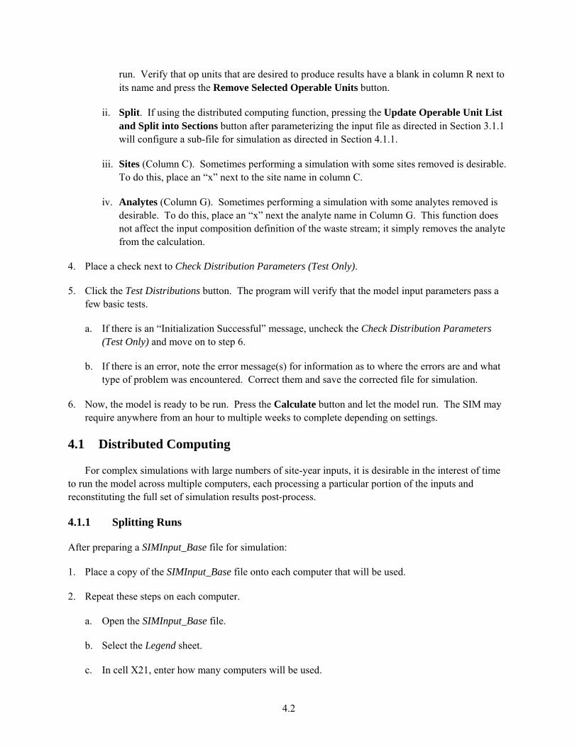
run. Verify that op units that are desired to produce results have a blank in column R next to its name and press the Remove Selected Operable Units button.

ii. Split. If using the distributed computing function, pressing the Update Operable Unit List and Split into Sections button after parameterizing the input file as directed in Section 3.1.1 will configure a sub-file for simulation as directed in Section 4.1.1.

iii. Sites (Column C). Sometimes performing a simulation with some sites removed is desirable. To do this, place an “x” next to the site name in column C.

iv. Analytes (Column G). Sometimes performing a simulation with some analytes removed is desirable. To do this, place an “x” next the analyte name in Column G. This function does not affect the input composition definition of the waste stream; it simply removes the analyte from the calculation.

4. Place a check next to Check Distribution Parameters (Test Only).

5. Click the Test Distributions button. The program will verify that the model input parameters pass a few basic tests.

a. If there is an “Initialization Successful” message, uncheck the Check Distribution Parameters (Test Only) and move on to step 6.

b. If there is an error, note the error message(s) for information as to where the errors are and what type of problem was encountered. Correct them and save the corrected file for simulation.

6. Now, the model is ready to be run. Press the Calculate button and let the model run. The SIM may require anywhere from an hour to multiple weeks to complete depending on settings.

4.1 Distributed Computing

For complex simulations with large numbers of site-year inputs, it is desirable in the interest of time to run the model across multiple computers, each processing a particular portion of the inputs and reconstituting the full set of simulation results post-process.

4.1.1 Splitting Runs

After preparing a SIMInput_Base file for simulation:

1. Place a copy of the SIMInput_Base file onto each computer that will be used.

2. Repeat these steps on each computer.

a. Open the SIMInput_Base file.

b. Select the Legend sheet.

c. In cell X21, enter how many computers will be used.

4.3

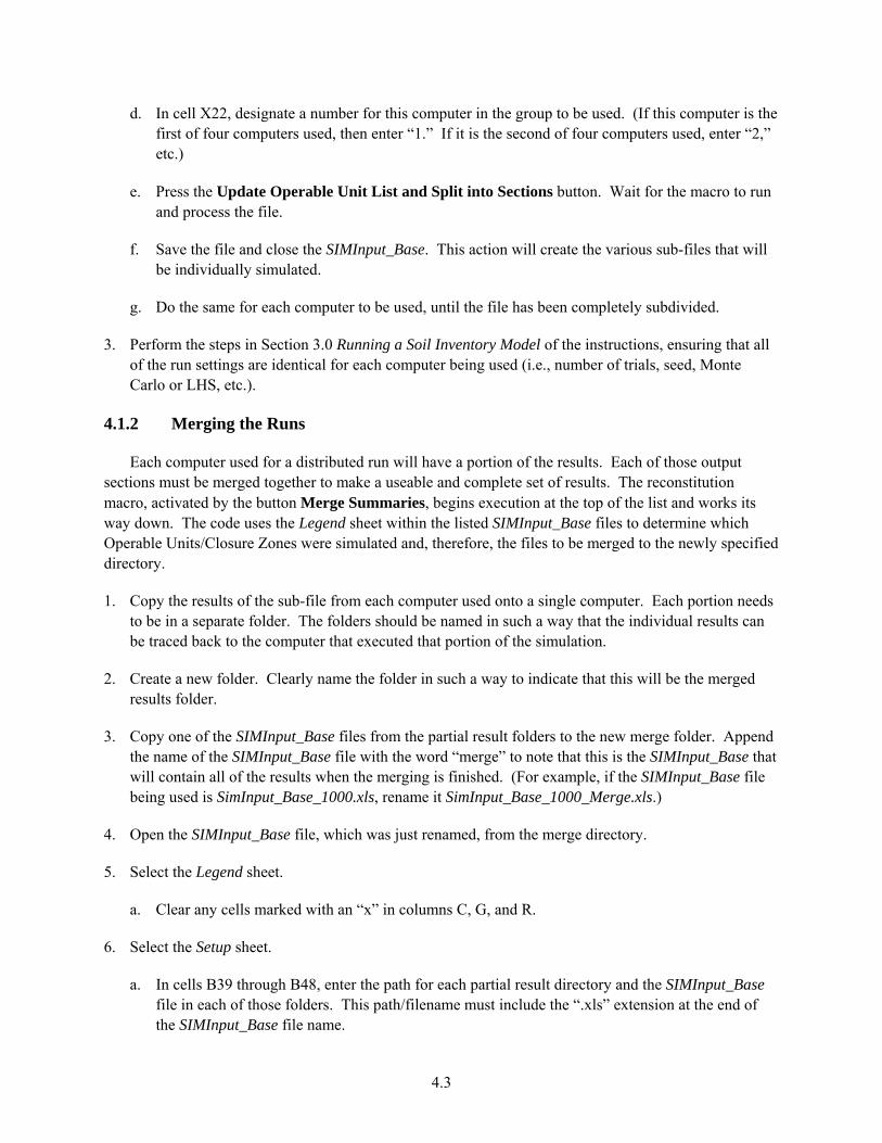
d. In cell X22, designate a number for this computer in the group to be used. (If this computer is the first of four computers used, then enter “1.” If it is the second of four computers used, enter “2,” etc.)

e. Press the Update Operable Unit List and Split into Sections button. Wait for the macro to run and process the file.

f. Save the file and close the SIMInput_Base. This action will create the various sub-files that will be individually simulated.

g. Do the same for each computer to be used, until the file has been completely subdivided.

3. Perform the steps in Section 3.0 Running a Soil Inventory Model of the instructions, ensuring that all of the run settings are identical for each computer being used (i.e., number of trials, seed, Monte Carlo or LHS, etc.).

4.1.2 Merging the Runs

Each computer used for a distributed run will have a portion of the results. Each of those output sections must be merged together to make a useable and complete set of results. The reconstitution macro, activated by the button Merge Summaries, begins execution at the top of the list and works its way down. The code uses the Legend sheet within the listed SIMInput_Base files to determine which Operable Units/Closure Zones were simulated and, therefore, the files to be merged to the newly specified directory.

1. Copy the results of the sub-file from each computer used onto a single computer. Each portion needs to be in a separate folder. The folders should be named in such a way that the individual results can be traced back to the computer that executed that portion of the simulation.

2. Create a new folder. Clearly name the folder in such a way to indicate that this will be the merged results folder.

3. Copy one of the SIMInput_Base files from the partial result folders to the new merge folder. Append the name of the SIMInput_Base file with the word “merge” to note that this is the SIMInput_Base that will contain all of the results when the merging is finished. (For example, if the SIMInput_Base file being used is SimInput_Base_1000.xls, rename it SimInput_Base_1000_Merge.xls.)

4. Open the SIMInput_Base file, which was just renamed, from the merge directory.

5. Select the Legend sheet.

a. Clear any cells marked with an “x” in columns C, G, and R.

6. Select the Setup sheet.

a. In cells B39 through B48, enter the path for each partial result directory and the SIMInput_Base file in each of those folders. This path/filename must include the “.xls” extension at the end of the SIMInput_Base file name.

4.4

b. Press the Merge Summaries button. Verify that the macro is ready to run when the dialog boxes appear. Wait for the macro to finish executing.

c. If an error message appears at this point, verify the directory paths to each partial result, ensuring that the SIMInput_Base file that is currently open has had its name appended and is from the new merge folder. Clear the merge folder except for the SIMInput_Base file that is open, fix any error(s), and run the macro again.

7. Save and close the open SIMInput_Base file that was appended with the word “merge.” This SIMInput_Base is now the file of record for this set of results.

5.1

5.0 Quality Assurance and Error Recovery Guidance

There are several different macro testing codes that are used to evaluate the performance of the simulation and to confirm that SIM executed correctly. These codes test the stability of the Monte Carlo calculation (Convergence), run a test calculation on a selected site-analyte combination (Evaluate Top 10 List), run a series of separate qualifying calculations for convergence and arithmetic performance on a variety of different sites with different parameters (Blackboxtest_1), examine the waste volumes associated with a series of years or waste streams (VolumeBalance), and evaluate the model results with documented reference values at various levels of resolution (cCDI Database Query; Model Granularity; and Specific Analyte Comparison).

5.1 Convergence

Convergence testing ensures repeatability and stability of the model operation and the results produced. Development of convergence criteria is user defined. The results for the Hanford SIM include evaluations at the 5% and 10% deviation rate for the selected percentiles/outcomes (mean, median, standard deviation, 0.5th percentile, 5th percentile, 95th percentile, and 99.5th percentile). Corbin et al. (2005) discusses and illustrates the convergence testing protocol that was used. Perform the following steps to complete convergence testing:

1. Create a new folder and place a copy of the convergence testing Excel file into the new directory.

2. Open the convergence file. (Convergence)

3. Open the SIMInput_Base used to generate results.

4. Select the Legend sheet. Copy the list of the operable units (in cells Q2 to the bottom of that list), and copy them.

5. Using the open copy of the convergence file; paste the operable unit list into cell B8.

6. Close the SIMInput_Base file. (Do not save.)

7. Specify the directory path for each result set in cells B1 through B5. The end of the directory path must end with the “\”. At least two directories must be specified, and up to five sets of results can be used. Using five different sets of results is recommended to verify repeatability.

8. Press the Run Convergence button and wait for the macro to finish. This action can take several hours.

9. The results from this test are reported in columns F through M of the Convergence worksheet file.

10. The corrected convergence values for identified/specified small number errors are listed in cells K60 to K62.

5.2

When the convergence macro is completed, ensure that each “drop” line on the graph produced approximately aligns with other lines. If one of the “drop” lines behaves substantially differently than the others (if that “drop” is much lower then the others and is by itself), then note which run was removed from that comparison and track that run to the computer used.

That type of quantitative behavior from the test indicates either:

1. Potential hardware errors were introduced in the simulation; or

2. A potential outlier run was generated coincidentally.

In either case, a new simulation should be run as part of the final results file, potentially on a different machine. If there is an interest in the results of a specific operable unit, each operable unit has a file created which contains the entire individual site comparisons run for that operable unit.

5.2 Top 10 Lists

This tool uses the three top 10 lists for each analyte for a particular simulation as a basis for evalu-ation. The first list is determined by the highest mean inventory (Column A thru Column H). The second is determined by the greatest median inventory (Column I thru Column P). The third list consists of the sites with the highest relative standard deviation (Column Q thru Column X).

The SiteEval (Site Evaluation) spreadsheet is a diagnostic tool that allows investigation of a specific analyte inventory at a particular site in the Top 10 list. Selecting the site name a list and pressing the Evaluate Top 10 List button at the top of the page runs a Crystal Ball simulation for that one analyte for that site for all years that the site received waste. On activation of the Evaluate Top 10 List macro, the SiteEval worksheet will be populated with the model input parameters and uncertainty definitions for that site-analyte combination and run a conventional Crystal Ball Monte Carlo scenario so that the individual contributing elements to the total inventory can be evaluated. However, the SiteEval spreadsheet can only run one site-analyte combination at a time on the Top 10 list, although multiple evaluation scenarios could be saved in a separate workbook if the user so desires.

Results will be shown on the SiteEval sheet of the SIMInput_Base file. Columns AN through AZ contain the Crystal Ball results for each waste stream and year contribution to the site total. The area formatted with a light yellow background in columns AS through AZ contain the results from the OCB-based SIM run for comparison purposes.

5.3 Blackbox Test

This test verifies that the results for sites with the ten highest relative standard deviations for each analyte and their associated median values are calculated the same by Crystal Ball and by OCB. The Test_BlackBox1 macro command performs an independent test of the OCB results by running the Top 10 list outputs for the relative standard deviation results comprehensively through the Evaluate Top 10 List macro and compares those results to the output obtained using regular Crystal Ball. The results are reported to the BlackBoxTest1 sheet. This test is done as an internal QA consistency check to establish that the model parameters and computation commands are functioning correctly, the calculations are being performed correctly, and as a second check on satisfying the convergence criteria.

5.3

This test serves as a double check for the validity of the OCB results by verifying the outcomes of the calculations using a different piece of software and evaluating the results to ensure that they are within the user defined quality assurance tolerances. If the Crystal Ball based outcomes for relative standard deviation or median are substantially different for any of the site-analyte combinations, then that result is counted as an error. As a result of the intrinsic modeling variability of these sites and the associated possible small number errors, perfect agreement between the OCB results and Crystal Ball is not expected. Error rates will vary depending on parameterizations used in the model and the error tolerance incorporated as part of this test is a function of the user requirements.

1. Open the SIMInput_Base file located in the results directory.

2. Press Alt-F8 to bring up the run macro dialog box. (This can also be done through Tools menu-> Macro -> Macros.)

3. Select Test_Blackbox1, and press run.

4. In the first dialog box, enter 1 and press “OK.”

5. In the second dialog box, enter 1, and press “OK.”

6. This process will take approximately 5 days to complete on a computer with the recommended hardware and software configuration with the same simulation parameterizations. The results will be reported in columns A-H.

7. When completed, select the BlackBoxTest1 sheet.

a. The number of results that fall out of the specified tolerance for relative standard deviations and medians (in this case, 5%) is found in cells M10 and N10 respectively.

b. The total error rate for relative standard deviation and median are listed M11 and N11, respectively.

5.4 Volume Balance Macro

The volume balance macro is a diagnostic tool that allows for the checking of volumes used in the SiteInput. It provides a compact way of reviewing the total volumes of waste discharged in three ways: by waste stream as a function of time; by year, with each total waste stream contribution; and by total waste stream volume. Thus, waste losses can be reconciled and allocated to the proper time and amount. This worksheet aids in enforcing the overall mass balance boundary condition and can assist in evaluating analyte solubilities and volume percent solids lost.

1. Beginning with an open SIMInput_Base, press Alt-F8 to bring up the macro selection window (or access via the Tools menu -> Macro -> Macros).

2. Select volume balance from the list of macros and press the run button. Wait briefly for the macro to finish executing.

3. Results will be written to the VolumeBalance sheet in the SIMInput_Base file.

5.4

This macro provides three sets of results. The first set of columns (A through C) shows the total volume of each waste stream discharged by year. The next set of columns (E through G) shows the total volumes discharged each year of the model as a function of waste stream. The last set of columns (I through K) displays the sum of the total volume mean values used for each waste stream, providing a comprehensive volume discharge estimate.

5.5 Other QA and Error Recovery Tests

There are a variety of macro commands that assemble specific sets of SIM results to compare to reference values at differing levels of resolution. The results of these comparisons are then written to the appropriate worksheets within the SIMInput_Base file. The principal evaluation command is: cCDIcompare.

1. Open the current SimInput_Base file.

2. Navigate to the most current series of operable unit workbook files.

3. Select the operable unit workbooks that have comparable reference data and open them all.

4. Press Alt-F8 to bring up the macro selection window (or access via the Tools menu -> Macro -> Macros).

5. Select cCDIcompare from the list of macros and press the run button. Wait briefly for the macro to finish executing.

6. Results will be written to the cCDIDatabaseQuery, the individual cCDI analyte comparison sheets (Pu239, U238, Cs137, and Sr90), and the 0,1,2 compare) in the SIMInput_Base file and comparison metrics developed.

This macro command has several subroutines that execute when this global macro is activated (Zero_0_1_compare, insertlessthansfor_blues, and insertlessthansfor_bluesandgreens). These commands can be executed individually, through the Tools menu, but are usually done as part of the overall comparison testing.

The cCDIcompare macro will populate the specified cells in the various worksheets for evaluation and the results of the comparisons are tabulated and reported. The 0,1,2 compare worksheet provides global and rolled up high level comparisons with regard to the site categories. The specific analyte comparisons for Pu-239, U-238, Cs-137, and Sr-90 worksheets have the resulting simulation percentile values and the comparisons reported in them. These results are also consolidated in the cCDIDatabaseQuery worksheet using the lessthan worksheet as part of the comparison process.

Subroutines (insertlessthansfor_blues, and insertlessthansfor_bluesandgreens) in the macro modify the comparison metrics appropriately so as not to penalize the model performance. Additionally, the comparisons require a one to one correspondence for the comparisons to be valid. Thus, a site that does not have an inventory estimate from Diediker (1999) for one of the analytes is excluded from this evaluation and any further quantitative comparisons. Cells colored blue are the “less than” values included in Diediker (1999); cells colored light green are the “less than” values found in other source

5.5

documents that were not carried forward as “less than” values. Other cells, shaded yellow, highlight corrections to the supplied data that were incorporated as part of this comparison. These corrections have been incorporated and documented as part of Table 6-32 in Section 6.0 of Corbin et al. (2005).

The simulation results for a site are compared with the information from specific reference data and the number of reference data values Diediker (1999) that fall within the 99th percentile range are counted as agreement. Simulation results that disagree with the reference data are counted and qualified as out-of-range either high or low.

6.1

6.0 SIM Outputs

The results generated by SIM are written to the results folder specified in the Setup worksheet, with the number of individual workbooks dictated by the Legend worksheet. There are two places SIM-created outputs can be found depending on the level of resolution needed: the individual category (operable unit) workbooks in the Results folder have the comprehensive results for each site-analyte-year result; and the SimInput_Base file has a variety of summary level results compiled in various worksheets (Top 10 List; SumFrcLiq, SumFrcSol; SumFrcTot). Other outputs are generated as a result of executing macro commands after SIM has been completed (e.g., the SACOutput).

6.1 Category (Operable unit) Workbook Results

The comprehensive SIM outputs are reported in separate workbooks organized by category as specified by the user. In the case of the Hanford SIM the selected category designation was operable unit. They are created and populated automatically by OCBHanford in the folder designated in the Setup worksheet, with multiple model runs of the same input file assigned separate folders (Results001, Results002, etc.). The site grouping organization in the Legend can be constructed using any number of desired criteria; however, care must be taken to ensure that no output file exceeds the maximum length of an Excel worksheet (65,536 rows); otherwise, the computation will cause the computer to stall, and the code will not run to completion.

Each site-year-analyte-phase combination inventory result is reported along with total inventory results for each analyte by site and the comprehensive total for the operable unit. In addition, the input volume is described in terms of percentiles in order to derive a corresponding concentration percentile value for the site-year-analyte combination. Therefore, these concentration and volume percentile data are also calculated and are provided in the individual operable unit/closure zone results workbooks.

6.2 SAC Output Files

The category workbook outputs and consolidated results are useful in a variety of ways, from diagnosing systemic errors in modeling to evaluating specific site-year analyte results of interest. However, the Inventory Module used in SAC (Bryce et al. 2002; Kincaid et al. 2006) to evaluate groundwater contamination requires the SIM-generated inventories to be decoupled into concentration and volume components to be used as inputs. These components are generated concurrently and reported together with the inventories providing a comprehensive, consolidated quantitative description of the site-year analyte inventories, waste stream volumes, and aggregate waste compositions.

The previously described operable unit workbooks created by OCB cannot be used directly by the System Assessment Capability (SAC) model, thus reformatting the results is required to make them usable by the SAC. The Create SAC Output macro takes the specified set of output files in a directory and assembles them into a structure that can be directly read by SAC.

1. Open the SIMInput_Base file that resides with the results.

2. Select the Setup sheet.

6.2

3. Press the Create SAC Output button.

This macro will create two suitably sized SAC Output files (MS Excel workbook format) in a subdirectory to the current results directory that can be directly used by SAC.

6.3 Summary Inventory Spreadsheets

These summary spreadsheets (SumFrcTotal, SumFrcLiquid, and SumFrcSolid) are part of the SimInput_Base file. The labels are relatively self-explanatory: SumFrcTotal (summary, fraction total), SumFrcLiquid (summary, fraction liquid), and SumFrcSolid (summary, fraction solid). They provide the total inventory by category (e.g., operable unit) and the total site inventory (as a summary of the summations for each operable unit). As noted previously, the comprehensive site inventory summary results are not available if a distributed model is performed because the overall binning information is not carried over in that process, but the sum of the various mean values for the operable units is present.

6.4 Top 10 Lists Spreadsheets

The Top 10 lists are diagnostic tools and offer a high-level view of the overall model results. Its function is also self-explanatory—the Top 10 list provides a list of the site locations for the 10 highest total inventory and concentration values for each analyte. The values measured are mean inventory, median inventory, and relative standard deviation at the consolidated site level.

This series of results provides where the largest inventories for a particular analyte are and where the most uncertain inventory values are. From a diagnostic standpoint, this table allows for evaluation of significant systemic errors or patterns in the input that impact the output. From an overall view of the model results, the selected organization of the results is an efficient method for inspecting and evaluating the data. These data are useful to identify specific sites of greater risk and those where the application of potential mitigation strategies and resources is most warranted.

7.1

7.0 References

Agnew SF, J Boyer, RA Corbin, TB Duran, JR FitzPatrick, KA Jurgensen, TP Ortiz, and BL Young. 1997. Hanford Tank Chemical and Radionuclide Inventories: HDW Model Rev. 4. LA-UR-96-3860, Los Alamos National Laboratory, Los Alamos, New Mexico.

Bryce RW, CT Kincaid, PW Eslinger, and LF Morasch (eds.). 2002. An Initial Assessment of Hanford Impact Performed with the System Assessment Capability. PNNL-14027, Pacific Northwest National Laboratory, Richland, Washington.

Corbin RA, BC Simpson, MJ Anderson, WF Danielson, JG Field, TE Jones, and CT Kincaid. 2005. Hanford Soil Inventory Model, Revision 1. RPP-26744, Rev. 0, CH2M HILL Hanford Group, Inc., Richland, Washington.

Diediker LP. 1999. Radionuclide Inventories of Liquid Waste Disposal Sites on the Hanford Site. HNF-1744, Fluor Daniel Hanford, Inc., Richland, Washington.

Field JG and TE Jones. 2005. Tank Farm Vadose Zone Contamination: Volume Estimates for Risk Assessments. RPP-23405, Rev. 1, CH2M HILL Hanford Group, Inc., Richland, Washington.

Higley BA, DE Place, RA Corbin, and BC Simpson. 2004. Hanford Defined Waste Model, Rev. 5. RPP-19822, Rev. 0, CH2M HILL Hanford Group, Inc., Richland, Washington.

Iman RL and WJ Conover. 1982. “A Distribution-Free Approach to Inducing Rank Correlations Among Input Variables.” Communications in Statistics B11(3):311-334.

Kincaid CT, PW Eslinger, RL Aaberg, TB Miley, IC Nelson, DL Strenge, and JC Evans. 2006. Inventory Data Package for Hanford Assessments. PNNL-15829, Pacific Northwest National Laboratory, Richland, Washington.

Simpson BC, RA Corbin, and SF Agnew. 2001. Hanford Soil Inventory Model. BHI-01496, Rev. 0, Bechtel Hanford Inc., Richland, Washington.

Simpson BC, RA Corbin, MJ Anderson, and CT Kincaid. 2006. Hanford Soil Inventory Model (SIM) Rev. 1 Software Documentation Requirements, Design, and Limitations. PNNL-16098, Pacific Northwest National Laboratory, Richland Washington.

Watrous RA and DW Wootan, and SF Finfrock. 2002. Activity of Fuel Batches Processed Through Hanford Separations Plants, 1944 Through 1989. RPP-13489, Rev. 0, CH2M HILL Hanford Group, Inc., Richland, Washington.

PNNL-16099

Distr.1

Distribution No. of No. of Copies Copies OFFSITE 3 B.C. Simpson NuvotecUSA, Inc. 723 The Parkway Richland, WA 99352 ONSITE 20 DOE Richland Operations Office B.L. Charboneau A6-33

13 Pacific Northwest National Laboratory R.W. Bryce E6-35 P.W. Eslinger K6-52 M.D. Freshley K9-33 C.T. Kincaid (5) K9-33 G.V. Last K6-81 B.E. Opitz K6-75 M.B. Triplett K6-52 Hanford Technical Library (2) P8-55