PNNL-16098

Hanford Soil Inventory Model (SIM) Rev. 1 Software Documentation – Requirements, Design, and Limitations B. C. Simpson R. A. Corbin M. J. Anderson C. T. Kincaid September 2006 Prepared for the U.S. Department of Energy under Contract DE-AC05-76RL01830

DISCLAIMER This report was prepared as an account of work sponsored by an agency of the United States Government. Neither the United States Government nor any agency thereof, nor Battelle Memorial Institute, nor any of their employees, makes any warranty, express or implied, or assumes any legal liability or responsibility for the accuracy, completeness, or usefulness of any information, apparatus, product, or process disclosed, or represents that its use would not infringe privately owned rights. Reference herein to any specific commercial product, process, or service by trade name, trademark, manufacturer, or otherwise does not necessarily constitute or imply its endorsement, recommendation, or favoring by the United States Government or any agency thereof, or Battelle Memorial Institute. The views and opinions of authors expressed herein do not necessarily state or reflect those of the United States Government or any agency thereof.

PACIFIC NORTHWEST NATIONAL LABORATORY operated by BATTELLE

for the UNITED STATES DEPARTMENT OF ENERGY

under Contract DE-AC05-76RL01830

Printed in the United States of America

Available to DOE and DOE contractors from the Office of Scientific and Technical Information,

P.O. Box 62, Oak Ridge, TN 37831-0062; ph: (865) 576-8401 fax: (865) 576-5728

email: reports@adonis.osti.gov

Available to the public from the National Technical Information Service, U.S. Department of Commerce, 5285 Port Royal Rd., Springfield, VA 22161

ph: (800) 553-6847 fax: (703) 605-6900

email: orders@ntis.fedworld.gov online ordering: http://www.ntis.gov/ordering.htm

This document was printed on recycled paper.

PNNL-16098

Hanford Soil Inventory Model (SIM) Rev. 1 Software Documentation – Requirements, Design, and Limitations NuvotecUSA, Inc B. C. Simpson R. A. Corbin M. J. Anderson Pacific Northwest National Laboratory C. T. Kincaid September 2006 Prepared for the U.S. Department of Energy under Contract DE-AC05-76RL01830 Pacific Northwest National Laboratory Richland, Washington 99352

iii

Summary

The objective of this document is to support the simulation results reported by Corbin et al. (2005) by documenting the requirements, conceptual model, simulation methodology, testing, and quality assurance associated with the Hanford Soil Inventory Model (SIM). There is no conventional software life-cycle documentation associated with the Hanford SIM because of the research and development nature of the project. Because of the extensive use of commercial off-the-shelf software products, there was little actual software development as part of this application. This document is meant to provide historical context and technical support of Corbin et al. (2005), which is a significant revision and update to an earlier product Simpson et al. (2001). The SIM application computed waste discharges composed of 75 analytes at 377 waste sites (liquid disposal, unplanned releases, and tank farm leaks) over an operational period of approximately 50 years. The development and application of SIM was an effort to develop a probabilistic approach to estimate comprehensive, mass balanced-based contaminant inventories for the Hanford Site post-closure setting. A computer model capable of calculating inventories and the associated uncertainties as a function of time was identified to address the needs of the Remediation and Closure Science (RCS) Project.

In order to estimate mass balanced contaminant inventories and their uncertainties for the Hanford Site post-closure setting, a stochastic simulation method (a Monte Carlo-type calculation) was selected to provide estimates of inventory and uncertainty. Stochastic simulation was chosen because the modeling parameters for this calculation did not have satisfactory closed-form definitions to approach the problem from a purely mathematical standpoint; the available waste stream/site data were not sufficiently compre-hensive to apply regression analysis; and the desire for a comprehensive description of uncertainty eliminated sensitivity analysis as potential methods for analysis. Stochastic simulation is a broadly accepted modeling technique that meets the requirements of the task. Furthermore, there are substantial resources available to its application in practice; therefore, this method was used in developing SIM. In this approach, several options were considered for model development and the Open Crystal Ball (OCB) statistical package was selected in 2002.

The design of SIM is highly modular with separate data input (Microsoft Excel) and calculation engine (OCB.dll) files administered through an interface application that acquires the inputs, manages the data reporting, and creates the output files. This design method allowed for concurrent development of the individual model elements, increasing project efficiency. Each data input is considered an inde-pendent variable; therefore, the waste stream composition/properties and waste stream discharge histories for the waste disposal sites could be examined and developed using a variety of source data (e.g., historical process data, tank waste modeling, etc.) and assumptions without impacting other variables.

There are several limitations to the application of SIM. Principal among them is that history matching the model results with reference data was not a goal of SIM prior to publication of model results (e.g., Corbin et al. 2005); rather, history matching is an ongoing effort that relies on the interpretation of field characterization data. Intensive history matching is a proposed activity that is currently unfunded. Other limitations of the software are associated with the reliability and availability of input data, because the inputs used to generate the inventories using the SIM architecture are controlled by various independent organizations (Pacific Northwest National Laboratory; CH2M HILL Hanford Group, Inc.; and/or Fluor Hanford, Inc.), and because of the stability/appropriateness of the various physical and

iv

chemical assumptions used in quantifying model behavior. While an intensive history matching effort has not been undertaken, some limited comparisons between model results and historical data were performed. Accordingly, despite its limitations, the SIM results reported by Corbin et al. (2005) are the best available information on contaminant releases to the waste sites simulated.

A programmatic limitation of this effort is as a consequence of the software business environment there has been refinement and updating of OCB and Crystal Ball (CB), thus the SIM platform developed as part of the RCS Project and documented in Corbin et al. (2005) is not currently available software. There remains capability to do inventory calculations with this model with the current resources, licenses, and support from Decisioneering, however, acquiring additional licenses for the legacy version of OCB and CB in use in order to distribute the software is not possible.

v

Terms/Acronyms AMD advanced micro devices CB Crystal Ball CFL correction factors - liquid CFS correction factors - solid HDW Hanford Derived Waste (Model) GB gigabytes GHz gigahertz OCB Open Crystal Ball LHS Latin hypercube sampling MB megabytes ML megaliters PNNL Pacific Northwest National Laboratory QA quality assurance RAM random access memory RCS Remediation and Closure Science (Project) SAC System Assessment Capability SIM Soil Inventory Model UPS uninterruptible power supplies USB universal serial bus VBA Visual Basic for Applications

vii

Contents Executive Summary ............................................................................................................................ iii Terms/Acronyms................................................................................................................................. v 1.0 Project Requirements and Overview .......................................................................................... 1.1 1.1 Functional Requirement Description and Evaluation for SIM Task .................................. 1.1 1.2 Supplemental Project Implementation Decisions............................................................... 1.2 1.3 Hardware Requirements ..................................................................................................... 1.3 1.4 Software Requirements ...................................................................................................... 1.4 1.5 Project Requirements Translated to Software Requirements ............................................. 1.4 2.0 Mathematical Framework and Model Design ............................................................................ 2.1 2.1 SIM Conceptual Model ...................................................................................................... 2.3 2.2 Inventory Equation Descriptions........................................................................................ 2.3 2.3 Constraint Conditions of SIM ............................................................................................ 2.4 2.4 Model Input Data Requirements ........................................................................................ 2.5 2.5 SIM input Data Structure ................................................................................................... 2.6 2.5.1 Volume Definition and Parameterization................................................................ 2.8 2.5.2 Waste Stream Definition and Parameterization....................................................... 2.8 2.5.3 Density Definition and Parameterization ................................................................ 2.9 2.5.4 Correction Factors ................................................................................................... 2.10 2.6 Modeling Assumptions and Software Performance Limitations........................................ 2.10 3.0 Model Architecture..................................................................................................................... 3.1 3.1 Executable Modeling File .................................................................................................. 3.1 3.2 Visual Basic for Applications (VBA) Simulation Management Macros ........................... 3.3 3.3 Model Approach for Computing and Reporting Output .................................................... 3.3 4.0 Software and Modeling Quality Assurance Testing ................................................................... 4.1 4.1 Distribution Integrity Verification ..................................................................................... 4.1 4.2 Model Methodology Testing.............................................................................................. 4.1 4.3 Quality Assurance Testing ................................................................................................. 4.2 4.3.1 Convergence Testing............................................................................................... 4.3 4.3.2 Computation Verification and Convergence Testing .............................................. 4.4 4.3.3 Testing Model Output ............................................................................................. 4.4 4.3.4 Model Hardware Testing......................................................................................... 4.5 5.0 SIM Outputs ............................................................................................................................... 5.1 6.0 References .................................................................................................................................. 6.1 Appendix A – Software Architectural Diagrams ................................................................................ A.1 Appendix B – Computer Hardware Testing Description.................................................................... B.1

viii

Figures 2.1 Monte Carlo Sampling vs. Latin Hypercube Sampling.............................................................. 2.2 3.1 Illustration of Calculation Sequence, Inventory Generation and Binning Process at

the Innermost Level .................................................................................................................... 3.4

Tables 1.1 Hardware Requirements for SIM Operation............................................................................... 1.3 2.1 Available Distribution Parameter Definitions ............................................................................ 2.6 2.2 SiteInput Worksheet Example .................................................................................................... 2.8 2.3 AnalyteInput Worksheet Example .............................................................................................. 2.9 2.4 DensityInput Worksheet Example .............................................................................................. 2.10 3.1 Relationships and Descriptions of SIM Files ............................................................................. 3.2 3.2 Model Trial Output Organization and Summary Statistical Bases............................................. 3.5

1.1

1.0 Project Requirements and Overview

The principal project requirement for the Soil Inventory Model (SIM) was to provide comprehensive quantitative estimates of contaminant inventory and its uncertainty for the various liquid waste sites, unplanned releases, and past tank farm leaks as a function of time and location at Hanford. A computer model capable of performing these calculations and providing satisfactory quantitative output represent-ing a robust description of its inventory and uncertainty for use in other subsequent models was identified to address the needs of the Remediation and Closure Science (RCS) Project. Other requirements were identified from the initial project guidance (DOE 1999):

• Using process chemistry models, historical records, and currently available field data to develop radionuclide and chemical inventories

• Focus on the priority list established through the System Assessment Capability (SAC); the solution should be able to increase the list of contaminants of interest as individual project needs and SAC requirements evolve

• Use probabilistic modeling to describe uncertainty

• Report inventory with standard deviations for the Hanford 100, 200, and 300 Areas

• Report inventory cases that represent maximum inventories associated with each specific waste type

• Reconcile field data and model predictions

This document is meant to provide historical context and technical support of Corbin et al. (2005), which is a significant revision and update to an earlier product, Simpson et al. (2001). The development of this software was completed under the RCS Project managed by Pacific Northwest National Labora-tory (PNNL). The application described in Corbin et al. (2005) is viewed to be a mature product and its documentation and other SIM efforts are now being conducted under the Characterization of Systems Project at PNNL. A companion report (Simpson et al. 2006) provides a user’s guide for the Hanford SIM.

This report describes the software, requirements, design and limitations of SIM. Neither the purpose nor the goal of this model required specific history matching for site inventories as part of this effort (i.e., model results are not fitted to published data). Disagreement of the model with reference values or inconsistent behavior between historically similar sites in the model or observed in the reference values are causes for further investigation with respect to the model system bases and the reference data. Evaluation of these disagreements is part of the error recovery guidance process.

1.1 Functional Requirement Description and Evaluation for SIM Task

The ability to use familiar, commercially available software on high-performance personal computers for data input, modeling, and analysis, rather than custom software on a workstation or mainframe

1.2

computer for modeling, was preferred. The proof-of-principle task documented in Simpson et al. (2001) led to the development and application effort described in Corbin et al. (2005).

Several quantitative tools/programs such as sensitivity analysis, multivariate statistical models, and stochastic simulation, were considered to represent the disposal situation at the Hanford Site and provide analysis of the contaminant inventories discharged to ground. Each modeling method that was evaluated had its advantages and disadvantages and they were evaluated in context for this particular application (Corbin et al. 2005).

Because the objective of this task is to provide an approach to estimate mass balanced inventories and their uncertainties for the Hanford Site post-closure setting, and appreciating the limitations of the other methods under consideration, a stochastic simulation technique was selected to provide estimates of inventory and its uncertainty.

Stochastic simulation (or Monte Carlo) models typically use random number generators to draw samples from probability distributions and perform calculations. The objective of this simulation method is to quantify the uncertainties of the dependent variables based on the assumed uncertainties of a set of independent variables, when the relationships between the dependent and independent variables are too complex for an analytical solution. This method was considered to be the most appropriate for the task presented, but this method also has its limitations:

• The independent variables identified in the analysis may not actually be independent.

• The probability distributions assumed for the independent variables are often subjectively assumed and may not reliably describe historical actions.

• The number of iterations necessary to provide statistically valid results for the simulation is usually not known a priori; therefore, an evaluation of the results to demonstrate model repeatability and stability is necessary.

1.2 Supplemental Project Implementation Decisions

Several stochastic simulation options were considered for model development and the Open Crystal Ball (OCB) statistical package (Decisioneering 2002) was selected. The OCB software provided an appropriate development platform with which to construct a model that could accommodate the scope and requirements associated with this task (e.g. compute the annual inventories and uncertainties for several hundred waste sites for 75 analytes over a 50 year timeframe, using approximately 200 waste streams to describe the various discharges that occurred).

Because there was no a priori method to determine a sufficient number of iterations for this model to ensure statistically valid and repeatable results, an experiment using a test file with a variety of distribu-tions was developed and tested for convergence behavior. This process allowed for determining a sufficiently rigorous number of iterations necessary for the SIM results to be stable and repeatable. A separate discussion regarding software testing, verification, and validation processes is presented in Section 4.0.

1.3

1.3 Hardware Requirements

Because of the desire to use conventional personal computers for this task, there are several hardware-based challenges that impede the execution of the model. These challenges are associated with reading and writing the input data, performing large numbers of computations, and managing the output data. Thus, operation of SIM is predominantly limited by the amount of available random access memory (RAM) provided in the computer. However, because the Windows XP Professional operating system (Version 2002, Service Pack 2) constrains RAM memory use to 1.3 gigabytes (GB), more RAM above this limit does not enhance performance. Table 1.1 details the minimum and recommended hardware necessary for SIM.

Table 1.1. Hardware Requirements for SIM Operation

Minimum Required Hardware to Operate/Execute SIM Recommended Hardware to Operate/Execute SIM

Intel Pentium 4, 2.53 GHz or greater system (SIM has not been tested on the AMD platform)

Several Intel-based Pentium 4 systems with a clock speed greater than 3.0 GHz; each system is a single processor, not dual or multi-processor based.

1 GB of RAM 2 GB of RAM 1 GB of free hard drive space 5 GB of free hard drive space Smaller than a 20” monitor Greater than a 20” monitor

PC Case with room for and operating at least 4 case fans

PC Case operating with the original equipment manufacturer’s installed fan

Uninterruptible power supplies (UPS) DVD-RW DVD-R USB mass storage drive

AMD = Advanced micro devices. GB = Gigabytes. GHz = Gigahertz. PC = Personal computer. RAM = Random access memory. SIM = Soil Inventory Model. UPS = Uninterruptible power supplies. USB = Universal storage bus.

Computers meeting the minimum requirements can be used to run SIM, but the run times for the simulations become exceedingly long. A complete converged model run (assuming a typical 2005 model configuration) using the recommended hardware configuration distributed over four computers takes over 100 hours of chronological time or over 400 machine-hours of computing time. Therefore, using a single machine to execute a simulation as defined would take nearly three weeks of continuous operation to complete.

The amount of time necessary to complete a simulation varies as a function of the number of trials, sites, and analytes being evaluated, but other than for relatively simple troubleshooting situations, these models are very demanding with regard to the amount of time they require to perform an analysis.

1.4

1.4 Software Requirements

These are the minimum off-the-shelf software requirements for performing calculations using the current SIM and its associated infrastructure:

• Windows XP Professional;1 provides the operating system for the computer

• Windows.NET 1.11 provides the application environment

• Crystal Ball2 v5.2 provides the ability to evaluate scenarios using macros as part of the quality assurance infrastructure

• Open Crystal Ball 2 (OCB.dll); provides the computational engine to perform the stochastic calculations

• C# interface (OCBHanford3); administers the simulation by managing inputs and outputs through OCB

• Microsoft Excel1 2000 (or later); user interface for data input/output and analysis.

A consequence of the software business environment has resulted in the refinement and updating of Crystal Ball and OCB in the marketplace, thus the developed SIM platform is not in alignment with the currently available software that was documented in Corbin et al. (2005). There remains capability to do inventory calculations with this model with the current resources, licenses, and support from Decisioneering; however, acquiring additional licenses for the legacy version of OCB in use to distribute is not possible.

1.5 Project Requirements Translated to Software Requirements

In summary, the Hanford SIM, Rev. 1, software requirements at a high level are

1. Use a Monte Carlo approach to achieve a probabilistic model.

2. Compute annual inventories, volumes, and waste concentrations.

3. Simulate 75 analytes including chemicals and radionuclides.

4. Simulate the period between Hanford Site startup and present day, more than 50 years of operation.

5. Simulate several hundred waste sites and unplanned releases using approximately 200 waste streams.

6. Be able to simulate 25,000 realizations.

1 Software product of Microsoft Corporation, Redmond, Washington. 2 Software product of Decisioneering, Denver, Colorado. 3 OCBHanford is part of the Hanford SIM model and not a vendor product.

1.5

7. Be able to accept the following parameter distributions: normal, triangular, lognormal, exponential, beta, gamma, zero (null), and unity.

8. Provide results decay correct to 1 January 2001.

9. Simulate and report the mean, minimum, maximum, standard deviation, median, and the following percentiles: 0.5%, 5%, 10%, 15%, 20%, 25%…85%, 90%, 95%, and 99.5%.

10. Compute the mass or activity of the liquid and entrained solids using the general equation

ssss CF*V*C* CF*V*C* I ρ+ρ= llll (1.1)

where: I = inventory ρ = density C = concentration V = volume CF = correction factor l = liquid s = entrained solid.

11. Employ a highly modular architecture with three principal elements: a C# interface code, an Open Crystal Ball calculation engine, and data input/output provided by MS Excel.

2.1

2.0 Mathematical Framework and Model Design

Stochastic simulation was the method chosen because the modeling parameters for this calculation did not have satisfactory closed-form definitions to approach the problem from a purely mathematical standpoint; the available waste stream/site data were not sufficiently comprehensive to apply regression analysis; and the desire for a comprehensive description of uncertainty eliminated sensitivity analysis as potential methods for analysis.

The theory underlying the Monte Carlo method of stochastic simulation used in SIM is briefly addressed in the following text. Monte Carlo is the method of approximating an expectation by the sample mean of a function of simulated random variables. It is about invoking laws of large numbers to approximate expectations. In mathematical terms, consider a random variable X having probability mass function or probability function fX(x) which is greater than zero on a set of values χ. Then, the expected value of a function g of X is:

(2.1)

if X is discrete and

(2.2)

if X is continuous. Now, if an n-sample of independently generated X’s, (a, b, c, …), and the mean of g(x) is computed over the sample, then that would result in the Monte Carlo estimate

of . (2.3)

Alternately, the random variable,

(2.4)

can be considered the Monte Carlo estimator of .

If exists, then the weak law of large numbers indicates that for any arbitrarily small є

(2.5)

2.2

This equation indicates that as n gets large, then there is a small probability that deviates much from . For the purposes of this task, the weak law of large numbers says that so long as n is large enough, arising from the Monte Carlo calculation shall be as close to as desired. For further detail regarding Monte Carlo methods, a principal reference cited in the Crystal Ball documentation is Hammersley and Handscomb (1964).

There are several variations of stochastic calculations. In this case, OCB has two methods of simulation, Monte Carlo and Latin hypercube sampling (LHS). By selecting Monte Carlo, the calculation will proceed using a simple random sampling method. The random behavior in games of chance is similar to how the Monte Carlo simulation selects variable values at random throughout the selected probability distribution to simulate a model.

The LHS variation of this calculation works by segmenting the assumed probability distribution into a number of non-overlapping intervals, each having equal probability, as shown in Figure 2.1. Thus, LHS simulation can provide a faster convergence to a theoretical result than the simple random sampling Monte Carlo simulation for a given number of trials. However, demands on computing resources are higher for LHS (memory usage is higher and run-time performance is slower in the LHS simulation) and there is no guarantee of improvement (i.e., faster convergence).

Figure 2.1. Monte Carlo Sampling vs. Latin Hypercube Sampling

2.3

2.1 SIM Conceptual Model

The SIM conceptual model is relatively straightforward:

1. Review and select source data and model boundaries 2. Develop, configure, and test model inputs 3. Develop, administer, and perform model calculation/simulation 4. Report model calculation results 5. Perform model quality assurance and error correction on model 6. Refine model elements as necessary

Evaluation and execution of the conceptual model elements was often performed concurrently and iteratively during the development of SIM. The sequence of the following narrative sections presents how the implementation of the various portions of the concept increased in sophistication as the model evolved and not necessarily the linear progression of the model’s development.

2.2 Inventory Equation Descriptions

SIM is executing a basic equation that computes the mass or activity of a particular constituent. The general form of this equation is:

I = ρ*C*V*CF (2.6)

Inventory (I) = density*concentration*volume*correction factor

Because in some cases there are entrained solids included as part of the overall inventory, both liquid and solid phases of a waste stream must be computed, resulting in a slightly more complicated version of the equation:

I = ρl*Cl*Vt*(1-V%s)*CFL + ρs*Cs* Vt*V%s *CFS (2.7)

Inventory = density (liquid)*concentration (liquid)*total volume*(1-volume percent solids) + density (solids)*concentration (solids)*volume percent solids.

• Inventory is the calculated output and is reported in kilograms (kg) or curies (Ci).

• Density (ρl and ρs) is the bulk density used to describe each waste stream phase (liquid or solid) reported in g/mL.

• Concentration (Cl and Cs)is the analyte amount per unit mass in each waste stream phase reported in μg/g or μCi/g.

• Volume (Vt) is the total discharged amount reported in megaliters (ML).

• Volume percent solids (V%s) are the estimated or assumed solids’ contribution of a particular waste stream and are dimensionless.

2.4

• Correction factors applied to the liquid and solid phases (CFL and CFS) are the scalar multipliers used to provide inventory unit consistency. In this case the units in calculating the amounts for the chemicals result in kilograms, thus the correction factor is 1; the calculation for the radionuclides must be multiplied by 1E-06 to discount the inflation factor used to compensate for certain small radionuclide concentrations and provide output in Ci.

This form of the equation was selected based on the observed prevalence of the units associated with the analytical data, and these parameters are also presented in the Hanford Defined Waste (HDW) Model waste stream descriptions (Higley et al. 2004).

2.3 Constraint Conditions of SIM

The following list presents a short summary that the SIM system used as definitions, assumptions, and constraint conditions for modeling bases, data integrity, and uncertainty development. These modeling elements and their development are described in more detail in Corbin et al. (2005). Because of the flexible architecture of SIM, these constraint conditions can usually be modified or relaxed to accommodate specific situations or different environments as needed.

• The application of a minimum basis set of waste streams is assumed to be appropriate and sufficient to describe disposal site inventories.

• Waste management procedures and operating conditions are (or have been) reasonably consistent throughout Hanford Site processes.

• Comprehensive waste stream compositions, such as HDW Rev. 5 waste stream definitions (Higley et al. 2004) were used where possible and analyte correlations were maintained.

• Waste streams are charge balanced and site inventories are strictly non-negative; simplicity in describing waste stream-waste site input allocations/contributions was maintained throughout model development, within known physical/chemical limits.

• The model parameters do not have any intrinsic behavior that is highly extreme (e.g., asymptotically or discontinuously approaching zero or infinity).

• Contamination control measures and physical constraints in place generally prevented the loss of solids from the tank-canyon system.

• Waste stream compositions are as independent as practicable and minimize direct circularity in applying reference data values to modeling inputs.

• Alignment with available surveillance data with regard to waste stream-disposal site volume assignments and inventory values is maintained where possible.

• Alignment with Hanford tank farms regarding HDW stream compositions and chemistry assumptions is maintained, using contemporary sampling data sparingly.

2.5

• The mass balance assumption for the tank-canyon-disposal site system is enforced; thus, there are no losses assumed to the atmosphere.

• Logical extensions of contemporary waste stream data for analogous (but data sparse) situations in the absence of early Hanford Site surveillance information are used.

• The specified campaign subdivisions for the ORIGEN2 reactor production data (Watrous et al. 2002) are assumed to be appropriate groupings for defining uncertainty behavior as a function of time for the various radionuclides in each separation process and their associated discharges.

• The various input variables are assumed to be mathematically independent;

• The uncertainties defined for the radionuclide concentrations are assumed to be well described by the ORIGEN2 beta distribution curve-fits (radionuclides) and that they are not substantially confounded by solubility behavior.

• The inter-batch variability for a particular waste stream is assumed to be encompassed by the selected uncertainty definition.

2.4 Model Input Data Requirements

The data requirements dictate that the inputs used in SIM (site volumes, waste stream compositions, densities, etc.) can be appropriately assigned, quantitatively described using the available distributions, and are technically defensible. An assumption used in the SIM input files that is entered for use in OCB is the type of distribution and its corresponding quantitative description (e.g., expected value and range) for each independent variable (e.g. volume, density, concentration).

Each data input is considered an independent variable; therefore, the waste stream composition/properties and waste stream discharge histories for the waste disposal sites could be examined and developed using a variety of source data and assumptions that do not necessarily impact the other modeling variables. The references cited in Corbin et al. (2005) provide a broad spectrum of process engineering, modeling, and historical waste management data that were used in developing the inputs and represent a reasonable example of populating a model of this type.

Distributions for modeling parameters and their quantitative descriptions are assigned by a variety of methods. The distributions are then interpreted by the OCB.dll by the “distribution type” index and the associated parameters as seen in Table 2.1 (parameter 1, parameter 2, and parameter 3, which are different depending on the distribution). All input cells in the simulation control Microsoft Excel spreadsheet must be filled with the appropriate values to define a distribution, or if a distribution does not use three parameters, zero (0) must be entered in the remaining cells to allow the simulation calculations to proceed.

2.6

Table 2.1. Available Distribution Parameter Definitions

Distribution Type Index

Distribution Name Parameter 1 Parameter 2 Parameter 3

0 Normal Mean Standard deviation 0 = unconstrained; value = low cut-off

1 Triangular Minimum Mode Maximum

4 Lognormal Mean Standard deviation 0 = unconstrained; value = high cut-off

6 Exponential Rate 0 = none 0 = none

8 Weibull Location Scale Shape

9 Beta Alpha Beta Scale

12 Gamma Location Scale Shape

17 Zero (null) 0 0 = none 0 = none

18 1 (unity) 1 0 = none 0 = none

For a greater understanding of each type of distribution and their definition, refer to Decisioneering’s Crystal Ball 2000 User Manual (Decisioneering 2000) or their website at http://www.decisioneering.com.

2.5 SIM input Data Structure

The SIM has an input data structure represented as a series of matrices. These matrices use MS Excel worksheets as a user interface for data input. This section provides guidance on where the variables reside in the user interface. There are four worksheets used to collect and organize input data in the SIM production workbook (i.e., SimInput_Base) workbook. They are named SiteInput, AnalyteInput, DensityInput, and CorrFactors and are listed below to the right of the input matrices. These worksheets contain the quantitative information describing the input values and the corresponding distribution definitions used in the model. They represent the basis for calculation.

Model Input Matrix Workbook Location CL(i,k): concentration liquid matrix (μg/g or μCi/g); AnalyteInput worksheet CS(i,k): concentration solid matrix (μg/g or μCi/g); AnalyteInput worksheet TV(j,k,l): total volume matrix (ML); SiteInput worksheet VP(j,k, l): volume percent solids matrix (%); SiteInput worksheet CFL(i): correction factor liquid matrix; CorrFactor worksheet CFS(i): correction factor solid matrix; CorrFactor worksheet DL(i,k): density liquid matrix (g/mL); DensityInput worksheet DS(i,k): density solid matrix (g/mL); DensityInput worksheet

2.7

i = number of chemicals or radionuclides; i=1,imax imax = 75 analytes j = number of sites; j=1,jmax jmax = 377 total sites k = number of waste streams; k=1,kmax kmax = 196 waste streams l = years of operation l = 1944, lmax lmax = 2001 calendar year

The inventory calculations follow the example below and illustrate the correspondence of how the matrices relate to Equation 7 as part of executing the Monte Carlo simulation. Each parameter has an input distribution for each i, j, k, and l that serve as inputs to the simulation. A random selection from each independent input distribution is then used to calculate inventory and the resulting output matrices are computed.

FL(i,j,l,): inventory forecast liquid matrix for a specific site-analyte-year calculated over a waste stream, k (kg or Ci);

FL(i,j,l) = CL(i,k) *DL(i,k) * TV(j,k,l) * [1-VP(j,k,l)] * CFL(i) (2.8)

FS(i,j,l): inventory forecast solid matrix for a specific site-analyte-year calculated over a waste stream, k (kg or Ci);

FS(i,j,l) = CS(i,k) * DS(i,k) * TV(j,k,l) * VP(j,k,l) * CFS(i) (2.9)

FT(i,j,l): inventory forecast total matrix for a specific site-analyte-year calculated over a waste stream, k for both phases (kg or Ci);

FT(i,j,l) = CL(i,k) * DL(i,k) * TV(j,k,l) * [1-VP(j,k,l)] * CFL(i) + CS(i,k) * DS(i,k)*TV(j,k,l) * VP(j,k,l) * CFS(i) (2.10)

These next equations illustrate the comprehensive inventory forecast calculations over all contrib-uting waste streams for a site-analyte-year. The binning of the various outcomes to determine the fore-casted results for each analyte, site, year, and operating history is described in more detail in Section 3.3.

Deterministically:

FLi,j,l = CFLi * (Σk CLi,k*DLi,k* TVj,k,l* [1-VPj,k,l]) (2.11)

FSi,j,l = CFSi * (Σk CSi,k*DSi,k* TVj,k,l* VPj,k,l) (2.12)

FTi,j,l = FLi,j,l + FSi,j,l (2.13)

Stochastically:

FLi,j,l,t = CFLi * (Σk CLi,k,t *DLi,k,t * TVj,k,l,t * [1-VPj,k,l,t]) (2.14)

FSi,j,l,t = CFSi * (Σk CSi,k,t *DSi,k,t * TVj,k,l,t * VPj,k,l,t) (2.15)

2.8

FTi,j,l,t = FLi,j,l,t + FSi,j,l,t (2.16)

Where t = one trial

2.5.1 Volume Definition and Parameterization

Volume input data were reviewed and modeling parameters developed (Corbin et al. 2005) for both total volume and volume percent solids. These definitions were converted into a standard electronic format, the SiteInput worksheet of the SIMInput_Base workbook. The volume assumptions are particular to the site, year, and waste stream that contributed to the inventory and vary between categories (e.g., liquid waste disposal volumes, unplanned releases, and tank farm leaks have different volume distribution assumptions associated with them). The complete data record used in the model includes the site label, year, waste stream label, total volume, and volume percent solids, which are entered in the subsequent columns of this worksheet, respectively. Input volumes are provided in megaliters (ML).

The waste site and waste stream indices correspond to the identification number in the Legend worksheet. The comprehensive volume definition (total volume and volume percent solids, waste stream assignments, their mean values, and their respective distribution descriptions) has quantitative infor-mation about the amount and uncertainty associated with a particular waste stream for each site-year combination. Each site has a unique combination of waste stream and year descriptions assigned. Table 2.2 provides an example of the structure of the volume input matrix.

Table 2.2. SiteInput Worksheet Example

Legend # Legend # Total Volume (ML) Vol % Solids

s w Site Year Waste Stream

Dist Type Parm 1 Parm 2 Parm 3

Dist Type Parm 1 Parm 2 Parm 3

1 45 200-E-100 1945 BiPO4 (BT1) Cool Wtr-Stm Cond

1 0.00219 0.00438 0.00657 17 0 0 0

65 50 216-A-19 1955 PUREX (P1) Cold Start

1 0.825 1.10 1.38 1 0.045 0.09 0.125

2.5.2 Waste Stream Definition and Parameterization

After the sites for analysis in SIM were selected, the waste streams necessary to compute inventory and uncertainty were defined. Each waste stream has its own qualitative and quantitative description derived from historical process engineering data, assumptions regarding the presence and behavior of various analytes, and the previously developed waste stream values in the HDW Model (Higley et al. 2004). The AnalyteInput worksheet in the SIM production workbook defines the quantitative information about concentration and uncertainty behavior, in μg/g or μCi/g, of a specific analyte (or radionuclide) within a waste stream. Table 2.3 presents an example of the structure of the AnalyteInput worksheet. The radionuclide values in the AnalyteInput worksheet are all inflated by a multiplicative

2.9

Table 2.3. AnalyteInput Worksheet Example

Legend # Legend #

Liquids Input Values (µg/g or μCi/g; radionuclides values are shown multiplied by 10e9 in this sheet

for use during simulation)

Solids Input Values (μg/g or μCi/g; radionuclide values are shown multiplied by 10e9 in this sheet

for use during simulation)

w a Waste Stream_ Unc Analyte Dist - Liquid Parm 1 Parm 2 Parm 3

Dist - Solid Parm 1 Parm 2 Parm 3

1 1 1C Evap (BT2) Na 4 8.99E+04 1.40E+04 3.43E+05 4 1.78E+05 2.77E+04 6.78E+05

factor of 1E+09 because the OCB.dll calculation engine cannot perform computations on values less than 1E-16; thus, this accommodation was made as part of the development process and the correction factor for the radionuclides is specified accordingly.

In the Hanford SIM, the chemical uncertainties were generally parameterized using the HDW Model-derived uncertainties for the various process waste streams and assigned a lognormal distribution. For the radionuclides, regression analysis was used in the curve fitting process involving the ORIGEN2 data (Watrous et al. 2002) to quantify the radionuclide uncertainty distributions/parameters as they changed over time. The curve fit algorithm in Crystal Ball was used to quantify the uncertainty parameters in a consistent and technically defensible manner.

These distributions were applied to the appropriate waste stream compositions for use in the stochastic simulation. Beta distributions were assumed for the radionuclides to best represent the data from ORIGEN2 for several reasons. They provide non-negative values throughout the data range, and they avoid certain mathematically extreme conditions (i.e., infinities). The ORIGEN2 data do not fit any distribution well; therefore, the beta distribution is as good as any other.

The described method was used for the Hanford SIM to maintain consistency throughout the model; however, the uncertainties associated with the analytes/radionuclides with respect to the individual waste streams compositions can be crafted and applied to the specific inputs as desired or as the available data may dictate.

2.5.3 Density Definition and Parameterization

The DensityInput worksheet of the SIM workbook defines the density of a specific waste stream in g/mL. In this case, the guiding assumption is that all analytes have the same density within a waste stream phase (e.g., a separate bulk density is assumed for solids and liquids in a waste stream); thus, the density will be defined only by the specific waste stream and phase. Sources for density information include the HDW Model (Higley et al. 2004), historical process engineering data, and subject-matter expertise.

The waste stream index corresponds to the identification number in the Legend worksheet with the waste stream label. The mean values and distribution definitions for the supernatants and the solids are defined in the subsequent columns. Table 2.4 presents an example of the DensityInput worksheet.

2.10

Table 2.4. DensityInput Worksheet Example

Legend # Supernatants Density (g/mL) Solids

Density (g/mL)

w Waste Streams—

Current Dist Type Parm 1 Parm 2 Parm 3 Dist Type Parm 1 Parm 2 Parm 3

1 1C Evap (BT2) 4 1.26 0.063 0 4 1.77 0.088 0

2.5.4 Correction Factors

The CorrFactors worksheet contains scalar values that are used to convert units of the analyte inventories calculated in SIM to those desired by RCS for use in their models. The unit basis for the chemical analytes allows the correction factor to be 1 for results to be reported in kilograms. The unit basis for radionuclides dictates that the correction factor be 1E-06 to provide for reporting results in curies, after correcting for the 1E+09 inflation factor applied to the inputs. The definition and application of the correction factors are discussed in more detail in Corbin et al. (2005).

2.6 Modeling Assumptions and Software Performance Limitations

There are several limitations associated with the modeling assumptions and software performance incorporated in SIM. Specific history matching between SIM results and documented reference values was not a goal of the modeling effort, although there was some history matching for certain site-analyte combinations done as part of the SIM development. The SIM system also includes other limitations:

• Physical and mathematical simplifications of the various behaviors and boundary conditions necessary to reasonably quantify the model in the software.

• Errors that come to light in interpretation of the historical process chemistry or site descriptions as a result of obtaining discovery information that refutes or illuminates unclear or undocumented disposal situations.

• Use of contemporary tank data to define solubility conditions.

• Acceptance of current technical conventions as part of the waste definition.

• Ambiguity on the part of the past-practice data collection and recording methods that established the baseline site inventory values.

Furthermore, the SIM software was not necessarily intended to correct discrepancies attributable to human error or historical inconsistencies in the reference data, although identification, analysis, and correction of errors is part of the review and quality assurance (QA) process as demonstrated in Table 6-32 of Corbin et al. (2005). These limitations are described more fully in Corbin et al. (2005).

3.1

3.0 Model Architecture

The design of SIM is highly modular with separate data input and executable files. There are three principal elements to the SIM system: OCBHanford, the OCB.dll, and the SIMInput_Base data work-book. The OCBHanford C# interface code directs communication between the OCB.dll calculation engine and the user interface and data input provided by MS Excel. A modular architecture was selected to allow for efficiencies in model development and evaluation. Additionally, because run-time perform-ance is a major constraint for models of this type, several design approaches were examined to optimize the speed of the simulation with regard to the available computing resources. A distributed computing feature with the ability to add or remove sites and analytes was developed for use in production to reduce the amount of time necessary to test and generate results.

The SIM computing user interface also has three distinct elements. The MS Excel production workbook (SIMInput_Base) has two of them—the Setup worksheet and the Legend worksheet; these worksheets provide an interface for the user to define the boundaries and reporting requirements of the simulation. MS Excel was used because there was the desire to use a familiar and broadly available interface for data input and analysis.

The other interface element is OCBHanford. It is accessed via a dialog box which activates the simulation. Once the parameters in the SIMInput_Base workbook are set, the specific workbook to be used must be opened using OCBHanford and the program will execute. The calculation will then proceed as directed and outputs generated until the simulation is completed or interrupted. Table 3.1 briefly describes the various elements, functions, and relationships of the SIM system. Appendix A presents a series of use case diagrams that illustrate the core SIM functions.

3.1 Executable Modeling File

SIM Rev. 1 uses the OCBHanford interface application to generate the various output files. It is the executable file containing the C# code that interfaces with the SIMInput_Base workbook, which contains all of the inputs and the OCB.dll, which creates the probability distributions and performs the inventory calculations. OCBHanford creates the output workbooks and manages the data reporting. The OCBHanford dialog box also presents a series of diagnostic data regarding simulation time and computing resources demand that can be useful in gauging hardware suitability and model parameter settings. More detailed discussion of the operation of OCBHanford is in the SIM User’s Guide (Simpson et al. 2006).

3.2

Table 3.1. Relationships and Descriptions of SIM Files

File/Sub-File (application) Function Reads from Sends to/Read by

SIMInput_Base/SiteInput (MS Excel)

Source data: waste site definition, waste stream identification, waste volumes, years of operation

None; fundamental input file

OCBHanford (Reads)

SIMInput_Base/AnalyteInput (MS Excel)

Source data: waste stream composition definition, solids and liquids

None; fundamental input file

OCBHanford (Reads)

SIMInput_Base/DensityInput (MS Excel)

Source data: waste stream density definition, solids and liquids

None; fundamental input file

OCBHanford (Reads)

SIMInput_Base/CorrFactors (MS Excel)

Source data: scalar adjustment for unit correction

None; fundamental input file

OCBHanford (Reads)

SIMInput_Base/Setup (MS Excel)

Source data: simulation control parameters with regard to program execution

None; fundamental input file

OCBHanford (Reads)

SIMInput_Base/Legend (MS Excel)

Source data: simulation control parameters with regard to source data involved

None; fundamental input file

OCBHanford (Reads)

OCBHanford C# Interface Executable file: simulation data management and program administration

SIMInput_Base/ SiteInput, AnalyteInput, DensityInput, CorrFactor, Setup, Legend

OCB.dll; C# interface directs OCB.dll to send results to various Operable Unit output files; reads inputs from SIMInput_Base and sends results to SIMInput_Base/ SumFrc/SolFrc/LiqFrc

OCB.dll Dynamically linked library: computational engine performing probabilistic inventory and uncertainty calculations

OCBHanford OCBHanford C# interface directs OCB.dll to send results to various Operable Unit output files

3.3

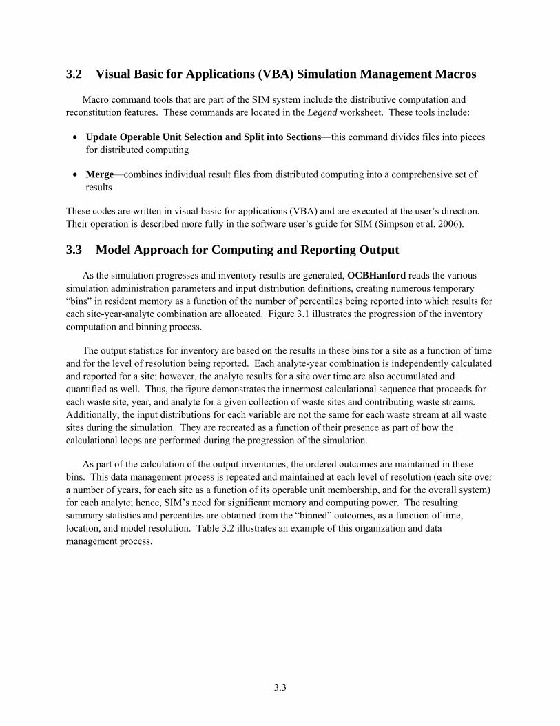
3.2 Visual Basic for Applications (VBA) Simulation Management Macros

Macro command tools that are part of the SIM system include the distributive computation and reconstitution features. These commands are located in the Legend worksheet. These tools include:

• Update Operable Unit Selection and Split into Sections—this command divides files into pieces for distributed computing

• Merge—combines individual result files from distributed computing into a comprehensive set of results

These codes are written in visual basic for applications (VBA) and are executed at the user’s direction. Their operation is described more fully in the software user’s guide for SIM (Simpson et al. 2006).

3.3 Model Approach for Computing and Reporting Output

As the simulation progresses and inventory results are generated, OCBHanford reads the various simulation administration parameters and input distribution definitions, creating numerous temporary “bins” in resident memory as a function of the number of percentiles being reported into which results for each site-year-analyte combination are allocated. Figure 3.1 illustrates the progression of the inventory computation and binning process.

The output statistics for inventory are based on the results in these bins for a site as a function of time and for the level of resolution being reported. Each analyte-year combination is independently calculated and reported for a site; however, the analyte results for a site over time are also accumulated and quantified as well. Thus, the figure demonstrates the innermost calculational sequence that proceeds for each waste site, year, and analyte for a given collection of waste sites and contributing waste streams. Additionally, the input distributions for each variable are not the same for each waste stream at all waste sites during the simulation. They are recreated as a function of their presence as part of how the calculational loops are performed during the progression of the simulation.

As part of the calculation of the output inventories, the ordered outcomes are maintained in these bins. This data management process is repeated and maintained at each level of resolution (each site over a number of years, for each site as a function of its operable unit membership, and for the overall system) for each analyte; hence, SIM’s need for significant memory and computing power. The resulting summary statistics and percentiles are obtained from the “binned” outcomes, as a function of time, location, and model resolution. Table 3.2 illustrates an example of this organization and data management process.

3.4

Figure 3.1. Illustration of Calculation Sequence, Inventory Generation and Binning Process at the Innermost Level

Trial 1

Trial 2

Random Volume

Random % Solids 1

Random Concentration 1

Random Density 1

Trial 1 Randomly Generated Inventory

To Memory: Stored as Trial 1

BINNING

Random Density 2

Random Volume

Random % Solids 2

Random Concentration 2

Trial 2 Randomly Generated Inventory

To Memory: Stored as Trial 2

Trial n

Random Volume

Random % Solids n

Random Concentration n

Trial n Randomly Generated Inventory

To Memory: Stored as Trial n

Random Density n

: :

3.5

Table 3.2. Model Trial Output Organization and Summary Statistical Bases

Site 216-X-001

Trial 1 Analyte Inventory

Result

Trial 2 Analyte Inventory

Result

Trial 3 Analyte Inventory

Result

Trial 4 Analyte

Inventory Result

Trial 5 Analyte Inventory

Result

Results for Year Summation Bin

(Fig. )

1961 a h o v ac a,h,o,v,ac…

1962 b i p w ad b,i,p,w,ad…

1963 c j q x ae c,j,q,x,ae…

1964 d k r y af d,k,r,y,af…

1965 e l s z ag e,l,s,z,ag…

1966 f m t aa ah f,m,t,aa,ah…

1967 g n u ab ai g,n,u,ab,ai…

Results for Site Summation Bin

T1 = a + b + c + d + e + f + g

T2 = h + i + j + k + l + m + n

T3 = o + p + q + r + s + t + u

T4 = v + w + x + y + z + aa + ab

T5 = ac + ad + ae + af + ag + ah + aj

T1, T2, T3, T4, T5,…T25,000

Thus, the percentile outcomes for a site over time (or the percentiles for a series of sites in a closure zone) cannot be simply summed and generate the resulting output distribution correctly, although summing the means over a series of years will provide the correct overall site mean. Each site-year-analyte outcome is analyzed over the number of selected trials and the resulting statistics generated. Furthermore, the distributive computing function prevents the creation of bins at the overall site level of resolution; thus, that series of comprehensive outputs can only be created running a complete simulation on a single machine.

4.1

4.0 Software and Modeling Quality Assurance Testing

A variety of tests dictated by good engineering practice and quality assurance were performed to ensure that SIM provides reliable output. The tests were directed at different issues relevant to the stability and calculation integrity of SIM and to determine the degree of agreement between the model estimates and the currently accepted inventory values.

4.1 Distribution Integrity Verification

A series of tests examined the performance of OCB and the associated distributions being used as part of SIM. These tests evaluated a variety of inputs and outputs using Crystal Ball and S-PLUS (an independent third-party stochastic software application marketed by Insightful Corporation) and created results as benchmark comparisons. These tests provide assurance that the individual uncertainty components used in the model are being correctly quantified.

The distribution verification test was performed to ensure that the OCB algorithms provide legitimate distribution definitions when compared to an independent third-party software package. All distributions available for use in SIM were evaluated. Varying parameterizations were defined and forecasts created in Crystal Ball and OCB. Similarly, these same distributions and outputs were created using S-PLUS. Each of these forecast outputs were then compared to each other to establish that the results generated by each software package were statistically indistinguishable (e.g., S-PLUS was compared with Crystal Ball; OCB was compared with Crystal Ball; and S-PLUS was compared with OCB).

4.2 Model Methodology Testing

The purpose of the methodology test is to establish that the method and parameters selected in modeling the system do not introduce bias and are consistent and repeatable within an acceptable tolerance. To accomplish this goal, an input test file that has a wide variety of component distributions with varying degrees of behavior and number of trials was used to establish the type of simulation (simple random sampling Monte Carlo vs. LHS) and to determine the model settings to be used for SIM and test various LHS size settings.

An initial determination regarding whether or not simple random sampling Monte Carlo analysis was appropriate for SIM was made. The tests conducted as part of Corbin et al. (2005) demonstrated that the simple random sampling Monte Carlo test file outputs do not show convergence at 25,000 trials. Because of this behavior, simple random sampling Monte Carlo analysis is not considered a viable option for SIM. After establishing that a conventional Monte Carlo modeling scenario using 25,000 trials will not satisfy model convergence requirements, the use of LHS simulation was investigated and found to provide acceptable results. Appropriate LHS modeling parameters were established to administer the simulation.

After completing several (e.g., up to five) separate runs for each parameterization for the test file, the results were checked for convergence at several selected points of the output probability distribution function (e.g., the mean, median, standard deviation, 2.5 percentile, 5 percentile, 95 percentile, and 97.5 percentile). These criteria established a 95th percentile range that was used as a metric for evaluation in this test. The convergence criterion for the SIM test file was set at this threshold: no more than 5% of

4.2

the individual analyte results could have deviations (percent differences) greater than 5%, using a maximum trial to trial variation on the selected outputs through the range. Mathematically, the deviations for each statistic were evaluated as follows:

Percent Difference = Max (S1…377 Y1…58 A1…75) – Min (S1…377 Y1…58 A1…75) Average [Max (S1…377 Y1…58 A1…75), Min (S1…377 Y1…58 A1…75)] (4.1) where S = site Y = year A = analyte

The results from these trials must demonstrate that the model as defined provides reproducible results within the convergence definition. The convergence test in this case was to quantify the differences between the maximum result and minimum result from any of the five runs over the average of the runs. The entire collection of outputs is evaluated for convergence as well as eliminating one trial, so that the outcomes for four out of the five outputs are graphed as well. Appendix B in Corbin et al. (2005) provides a comprehensive illustration of the process of identifying and determining convergence for a series of model results that was used to establish the use of LHS in the simulation.

This treatment quickly establishes the quantitative behavior of the model runs and allows for the detection of an outlier run. Once convergence as a function of the number of trials is verified, the results were compared against each other to find which of these settings gives the most consistent results. This set of output percentiles for the test file was selected to reduce the effect of small number error bias that has been observed in the left hand tail of the larger SIM file.

4.3 Quality Assurance Testing

There are elements of model verification and validation necessary as part of the quality assurance associated with this modeling effort. These requirements are not intrinsic to the development and execution of SIM but are separate activities necessary to maintain the technical integrity of the model and results produced. These requirements include ensuring that the code is executing the instruction set as desired (algorithmically), that the code is executing the instructions correctly (mathematically), and that there is a reasonable degree of agreement with observation or reference data using a quantifiable metric. The selected QA regimen includes testing model stability, calculation verification, and hardware inspection. These tests are performed post-simulation using macro commands or in the case of the hardware test, a specific executable file.

• Convergence—performs comprehensive trial-to-trial evaluation of SIM results to determine model stability and repeatability. There is a separate file and macro command that performs this test and reports the results.

• BlackBoxtest1—performs comprehensive check of selected Top 10 site-analyte list to perform calculation verification and as an additional check on the model convergence behavior. The results from this macro are reported in the SIMInput_Base workbook.

• cCDI Analyte Comparison—performs selected inventory comparisons between model results and reference values for particular sites. This macro command performs a series of comparisons at

4.3

various stages of resolution (including the 0,1,2 Compare test) and reports the results in the SIMInput_Base workbook.

• 0,1,2 Compare—performs selected inventory comparisons for groups of sites against the sums of reference inventory values. This macro can be performed on its own, but is usually performed as part of the cCDI Analyte Comparison.

• Site Evaluation—performs Crystal Ball evaluation of specific site-inventory using currently defined model parameters. It is usually run during the development and testing of model inputs. The results are not saved from run to run. The BlackBoxtest1 is a comprehensive, structured, application of this test.

• Volume Balance—performs global and year-by-year check on disposal site volumes for reconciliation with reference values.

4.3.1 Convergence Testing

Convergence testing was conducted to ensure that the comprehensive model results were repeatable within the convergence tolerance definition. This test does not measure error in the conventional sense (divergence from an accepted or known value); it only determines if the model parameters and model environment provide for stability in the results—returning statistically indistinguishable results for any selected model output. If this condition is observed, the number of iterations performed is considered to be satisfactory, and the modeling software and hardware are considered reliable.

This evaluation is similar in method and execution to the previous LHS qualification test, but with a different intent. In the prior series of tests, a test file was run to establish that the LHS parameters did not introduce a significant bias into the results. This test is significantly more rigorous in that it evaluates the results from five different model runs and illustrates the run-to-run behavior to determine model stability, establishing that the number of trials selected for the comprehensive model is indeed satisfactory.

Evaluation of the central tendencies, standard deviation, and tails were done for each site-analyte-year combination. The convergence definition in use for the comprehensive model is that no more than 5% of the results can have greater than 5% deviation within the 5th to 95th percentile ranges, inclusive (e.g., a 90th percentile output range), allowing for the observed bias of small numbers in the evaluation formula at the lower tail of the distribution.

The small number bias threshold for radionuclides was 1E-12 Ci (1 picocurie). This level was selected as a practical compromise that allowed for detection limits of the instruments/analytical methods and background interference. Results are also provided for the practical minimum (0.5th percentile) and maximum (99.5th percentile) returned by the SIM calculation. The minimum and maximum values are included in this series of evaluations, but are not used to establish whether convergence of the model was

4.4

achieved because they represent the most extreme conditions of the distribution, and the instability at the extremes (e.g., minimum and maximum values) is anticipated to be greater than the acceptance criteria, especially in the lower tail.

4.3.2 Computation Verification and Convergence Testing

In computation verification (e.g., black-box) testing, an input test file is evaluated based upon a number of specific SIM analyte and site combinations. This test determines the model stability for the most variable sites on two different bases: variability observed in relative standard deviation and median values. A Crystal Ball simulation is then run based on these parameterizations and a specific set of run preferences that match the OCB model parameters. Statistical output from this Crystal Ball test is then compared against the OCB output for the same analytes for each site.

The test file selected was the output Top 10 list from the production SIM run for all 75 analytes. The Site Evaluation macro was executed for each site-analyte combination for the highest relative standard deviation sites. The median and relative standard deviation for each site-analyte combination was then compared. The relative standard deviations were evaluated using a simple ratio of the black-box test result divided by the OCB result, where less than 95% is considered an error. The median was compared using a simple relative percent difference formula, where errors greater than 5% are noted and considered to be outliers.

4.3.3 Testing Model Output

An important project requirement and relevant QA comparison is to determine if the resulting overall model inventory estimates correspond to accepted literature estimates within a specified quantitative metric (e.g., global and individual model agreement with observation/reference data). This check serves as additional verification of the model performance. However, no comprehensive validation of SIM is currently possible because of the lack of independent field results. This comparison only incorporates data from where there is an accepted literature value in Diediker (1999) that was not determined to be in dispute with other historical information, for example, subject to correction for the presence of “less than” values in the reference literature.

For this comparison, a 99% estimate range of four analytes with reasonably comprehensive historical results (Cs-137, Sr-90, U-238, and Pu-239) was selected as the basis for comparison. Agreement is presumed between the model results and the accepted literature data if the literature result falls within SIM estimated 99% range. More sophisticated statistical tests are not warranted because the Diediker (1999) inventory values do not have an uncertainty definition.

Because of the lack of a comprehensive set of accepted reference values, there are no comparisons available for the tank leaks or most of the unplanned releases. Results for 179 of the 377 sites for each of the four specific analytes are provided in Corbin et al. (2005) at three different levels of model resolution (site-wide, operable unit, and site specific). The degree of agreement between model and observation using this metric for the selected specific sites and analytes is shown in Tables 6-3, 6-6, 6-7, 6-8, 6-9, and 6-31 of Corbin et al. (2005) for the four analytes.

4.5

4.3.4 Model Hardware Testing

The individual computers utilized for the simulations were tracked for performance using a test file, Memtest86 (http://www.memtest86.com), to ensure a controlled computing environment. Memtest86 is able to identify potentially unstable computing performance and allow the modelers to remove these machines from use in performing SIM calculations. Appendix B describes the various tests in more detail. These tests were allowed to run multiple times for each machine to ensure that the hardware was thoroughly tested. This testing is conducted before the SIM trials are run and after they are finished to ensure that simulation results do not suffer in quality and content validity from potential errors introduced by hardware malfunctions.

5.1

5.0 SIM Outputs

The individual category (Operable Unit) workbooks specified by the user in the Legend worksheet are created as defined in OCBHanford, with their respective sites, analytes, years, and categories. There can be as many output workbooks as there are sites being evaluated, however that structure is cumbersome because the number of workbooks created can be unwieldy. In the Hanford SIM there were logical groupings that existed and these were used to reduce the overall number of output files produced.

Additionally, as a function of producing the individual site-year-analyte results, summary analyte results were developed for the sites, analytes, and groupings over their operating lives resulting in a distribution for each for all the contributing years. Summary outputs for selected sites and each operable unit group are exported into their respective worksheets of the production SIMInput_Base workbook (SumFrcTotal, SumFrcSolid, SumFrcLiquid

Additionally, there is a post-process macro command used to generate SAC input files, Create SAC Output that creates a file that can be read and used directly by the SAC model. Other outputs created by the SIM post-process macro commands involve producing the results from the QA testing process. The execution of these macro commands will create or refresh results from a simulation (or series of simulations) in the production workbook (such as activating the VolumeBalance macro or the cCDI Analyte Comparision); or in a separate file as a result of executing the Convergence test macro.

6.1

6.0 References

Corbin RA, BC Simpson, and MJ Anderson (Nuvotec USA); WF Danielson III (Advanced Imaging Technologies); JG Field and TE Jones (CH2M HILL Hanford Group, Inc); and CT Kincaid (Pacific Northwest National Laboratory). 2005. Hanford Soil Inventory Rev. 1. RPP-26744, Rev. 0, CH2M HILL Hanford Group, Inc, Richland, Washington.

Decisioneering. 2000. Crystal Ball 2000 User Manual, Decisioneering, Inc., Denver, Colorado.

Decisioneering. 2002. Crystal Ball 2000 Software. Decisioneering, Inc., http://www.decisioneering.com, Denver, Colorado.

Diediker LP. 1999. Radionuclide Inventories of Liquid Waste Disposal Sites on the Hanford Site. HNF-1744, Fluor Daniel Hanford, Inc., Richland, Washington.

DOE-RL. 1999. Groundwater/Vadose Zone Integration Project Science and Technology Summary Description. DOE/RL-98-48, Vol. III, Rev. 0, U.S. Department of Energy, Richland Operations Office, Richland, Washington.

Hammersley JM and DC Handscomb. 1964. Monte Carlo Methods. Methuen & Co. Ltd., London, England.

Higley BA, DE Place, RA Corbin, and BC Simpson. 2004. Hanford Defined Waste Model, Rev. 5. RPP-19822, Rev. 0, CH2M HILL Hanford Group, Inc., Richland, Washington.

Simpson BC, RA Corbin, and SF Agnew. 2001. Hanford Soil Inventory Model. BHI-01496, Rev. 0, Bechtel Hanford Inc., Richland, Washington.

Simpson BC, RA Corbin, MJ Anderson, and CT Kincaid. 2006. Hanford Soil Inventory Model (SIM) Rev. 1 User’s Guide. PNNL-16099, Pacific Northwest National Laboratory, Richland Washington.

Watrous RA, DW Wootan, and SF Finfrock. 2002. Activity of Fuel Batches Processed Through Hanford Separations Plants, 1944 Through 1989. RPP-13489, Rev. 0, CH2M HILL Hanford Group, Inc., Richland, Washington.

Appendix A

Software Architectural Diagrams

A.1

Appendix A

Software Architectural Diagrams

The following use case architectural diagrams illustrate the essential modeling activities: generating soil inventories and reviewing/analyzing soil inventories.

Software Architectural Diagram A.1: Global SIM Use Case Diagram

This use case illustrates at the top level the interface of the scientist/user with the Soil Inventory Model (SIM) in either performing a simulation to generate inventory information, or in reviewing the results of the simulation to evaluate the performance of the model.

Software Architectural Diagram A.2: Generate Soil Inventory

This illustration demonstrates the interface of the user and model at the initial stage of executing a simulation. Several of the subsequent activity diagrams (A.3 through A.6.) show the interface of the scientist with SIM in finer detail with respect to generating inventory data.

A.2

Software Architectural Diagram A.3: Enter Simulation Data

The following activity diagram represents the sequence of activities for the user to enter simulation administration parameters for the model Setup and Legend sheets in the SIMInput_Base workbook. Specific guidance and instruction with regard to the identified activity blocks can be found in the SIM User’s Guide (Simpson et al. 2006).

A.3

Software Architectural Diagram A.4: Enter Site and Analyte Input Data

The following activity diagram represents the sequence of activities for the user to enter inventory calculation parameters for the model SiteInput and AnalyteInput sheets in the SIMInput_Base workbook. Section 2 of this document describes the processes involved in developing input data definitions. Specific guidance and instruction with regard to the identified activity blocks can be found in the SIM User’s Guide (Simpson et al. 2006).

A.4

Software Architectural Diagram A.5: Enter Density and Correction Factor Inputs

The following activity diagram represents the sequence of activities for the user to enter inventory calculation parameters for the model DensityInput and CorrFactors sheets in the SIMInput_Base workbook. Section 2 of this document describes the processes involved in developing these waste stream and inventory reporting data definitions. Specific guidance and instruction with regard to the identified activity blocks can be found in the SIM User’s Guide (Simpson et al. 2006).

A.5

Software Architecture Diagram A.6: Conduct Simulation

The following activity diagram represents the sequence of activities for the user to execute a simulation in order to calculate the soil inventory. Specific guidance and instruction with regard to the identified activity blocks can be found in the SIM User’s Guide (Simpson et al. 2006).

A.6

Software Architectural Diagram A.7: Review Inventory

This illustration demonstrates the interface of the scientist/user and model results at the initial stage of reviewing a simulation. The subsequent activity diagrams (A.8 and A.9) show the interface of the user with the model in finer detail with respect to reviewing inventory data.

A.7

Software Architectural Diagram A.8: Review Component and Total Inventory

The following activity diagram represents the where the summary result outputs for the solid, liquid, and total analyte inventories for a simulation are located in the SIMInput_Base workbook. Further description of SIM outputs and results can be found in Section 5.

A.8

Software Model Activity Diagram A.9: Review Top 10 and Operable Unit Inventory

The following activity diagram represents the flow of activity for reviewing output for the top 10 inventories by total mean, median, and standard deviation and by individual site-analyte-year inventories for a category (operable unit).

A.9

References

Simpson BC, RA Corbin, MJ Anderson, and CT Kincaid. 2006. Hanford Soil Inventory Model (SIM) Rev. 1 User’s Guide. PNNL-16099, Pacific Northwest National Laboratory, Richland Washington.

Appendix B

Computer Hardware Testing Description

B.1

Appendix B

Computer Hardware Testing Description

Memtest86 executes a series of numbered test sections to check for errors. These test sections consist of a combination of test algorithm, data pattern, and cache setting. The execution order for these tests was arranged so that data errors/hardware flaws will be detected as rapidly as possible from the highly obvious to the very subtle. A description of each of the test sections follows:

Test 0 [Address test, walking ones, no cache]

Tests all address bits in all memory banks by using an address pattern of walking ones. This test should find the most obvious hardware faults.

Test 1 [Address Test, Own Address]

Each address is written to memory with its own address and then is checked by the software for consistency. In theory, the previous test should have caught any memory addressing problems. This test should catch any additional addressing errors that somehow were not previously detected.

Test 2 [Moving Inversions, Ones and Zeros]

This test uses the moving inversions algorithm with patterns of all ones and zeros. The memory cache is enabled even though it interferes to some degree with the test algorithm. With cache enabled, this test does not take long and should quickly find all of the persistent or “hard” errors and some more subtle errors. This test is only a quick check.

Test 3 [Moving Inversions, 8 Bit Pattern]

This is the same as Test 1, but uses an 8-bit-wide pattern of "walking" ones and zeros. This test will better detect subtle errors in "wide" memory chips. A total of 20 data patterns are used.

Test 4 [Moving Inversions, Random Pattern]

Test 4 uses the same algorithm as Test 1 but the data pattern is a random number and its complement. This test is particularly effective in finding difficult to detect data sensitive errors. A total of 60 patterns are used. The random number sequence is different with each pass so multiple passes of Memtest86 increases the effectiveness of the test at locating errors.

Test 5 [Block Move, 64 Moves]

This test stresses memory by using block move (movsl) instructions. Memory is initialized with shifting patterns that are inverted every 8 bytes. Then, 4-MB blocks of memory are moved around using the movsl instruction. After the moves are completed, the data patterns are checked. Because the data are checked only after the memory moves are completed, it is not possible to know where the error occurred.

B.2

The addresses reported are only for where the bad pattern was found. Since the moves are con-strained to an 8-MB segment of memory, the failing address will always be less than 8 MB away from the reported address.

Test 6 [Moving Inversions, 32 Bit Pattern]

This is a variation of the moving inversions algorithm that shifts the data pattern left one bit for each successive address. The starting bit position is shifted left for each pass. To use all possible data patterns, 32 passes are required. This test is quite effective at detecting data sensitive errors, but the execution time is long.

Test 7 [Random Number Sequence]

This test writes a series of random numbers into memory. By resetting the seed for the random number, the same sequence of number can be created for a reference. The initial pattern is checked and then complemented and checked again on the next pass. However, unlike the moving inversions test, writing and checking can only be done in the forward direction.

Test 8 [Modulo 20, Ones and Zeros]

Using the Modulo-X algorithm in this test should uncover errors that are not detected by moving inversions due to cache and buffering interferences associated with that algorithm. As with Test 1, only ones and zeros are used for data patterns.

PNNL-16098

Distr.1

Distribution No. of No. of Copies Copies OFFSITE 3 B.C. Simpson NuvotecUSA, Inc. 723 The Parkway Richland, WA 99352 ONSITE 20 DOE Richland Operations Office B.L. Charboneau A6-33

13 Pacific Northwest National Laboratory R.W. Bryce E6-35 P.W. Eslinger K6-52 M.D. Freshley K9-33 C.T. Kincaid (5) K9-33 G.V. Last K6-81 B.E. Opitz K6-75 M.B. Triplett K6-52 Hanford Technical Library (2) P8-55