Embed Size (px)
Citation preview

Handwritten Digit Recognition using Convolutional Neural Networks in Python with Keras
Dr. Petra Kralj Novak
10.1.2019
https://machinelearningmastery.com/handwritten-digit-recognition-using-convolutional-neural-networks-python-keras/

Neural networks
Neuron, perceptron
The perceptron is a mathematical model of a biological neuron
• A single perceptron can separate linearly.
Output of P = {1 if A x + B y > C
{0 if A x + B y < = C
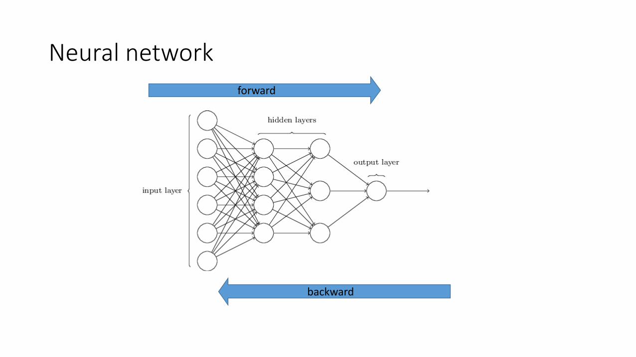
Neural network
forward
backward
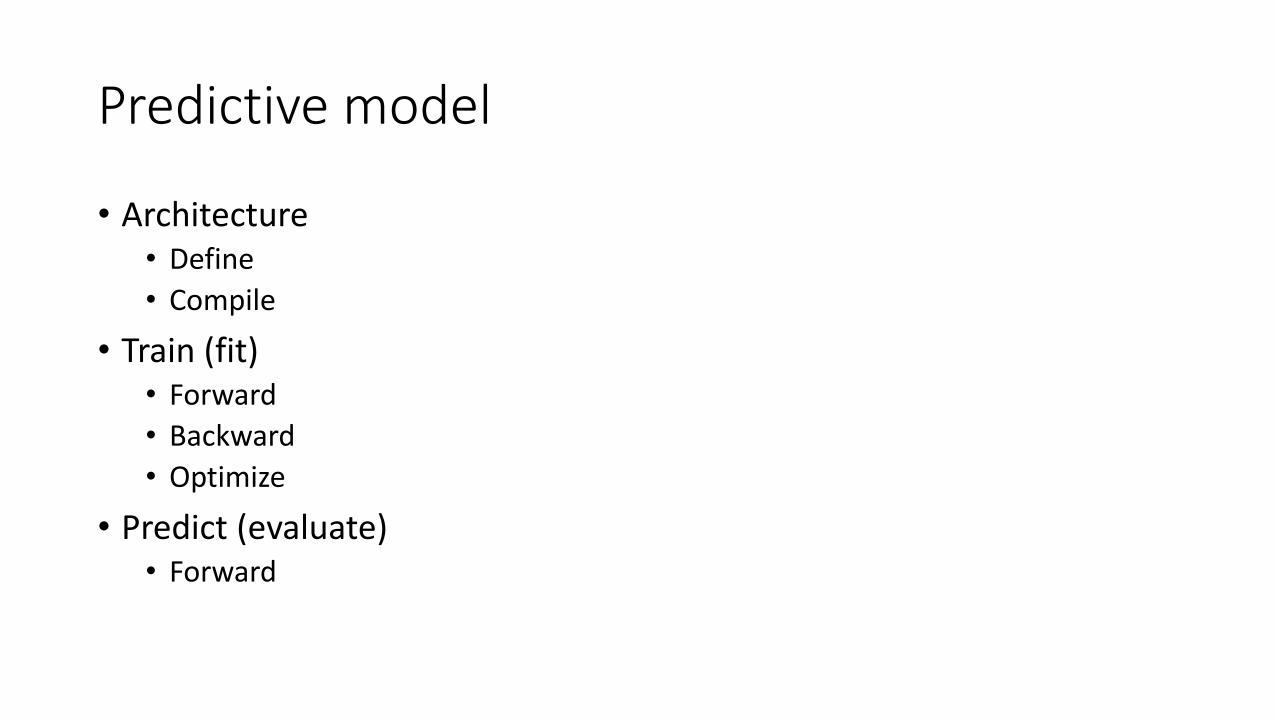
Predictive model
• Architecture• Define
• Compile
• Train (fit)• Forward
• Backward
• Optimize
• Predict (evaluate)• Forward
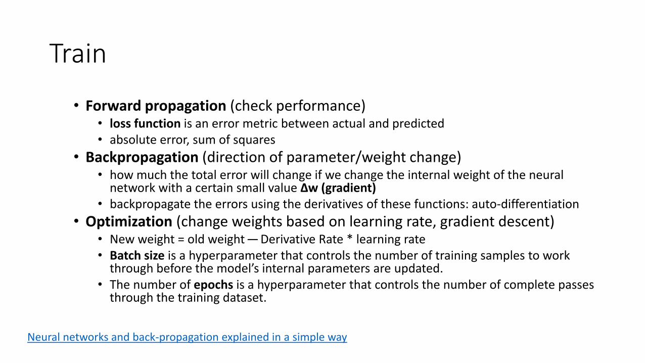
Train
• Forward propagation (check performance)• loss function is an error metric between actual and predicted• absolute error, sum of squares
• Backpropagation (direction of parameter/weight change)• how much the total error will change if we change the internal weight of the neural
network with a certain small value Δw (gradient)• backpropagate the errors using the derivatives of these functions: auto-differentiation
• Optimization (change weights based on learning rate, gradient descent)• New weight = old weight — Derivative Rate * learning rate• Batch size is a hyperparameter that controls the number of training samples to work
through before the model’s internal parameters are updated.• The number of epochs is a hyperparameter that controls the number of complete passes
through the training dataset.
Neural networks and back-propagation explained in a simple way
Keras: The Python Deep Learning library
• Keras is a high-level neural networks API, written in Python and capable of running on top of TensorFlow, CNTK, or Theano.
• Google’s Tensorflow: is a low-level framework that can be used with Python and C++.
• Install packages: tensorflow, keras

MINST – handwritten digits
• Each image is a 28 by 28 pixel square (784 pixels total).
• Normalized in size and centered
• A standard spit of the dataset is used to evaluate and compare models, where 60,000 images are used to train a model and a separate set of 10,000 images are used to test it.
Exercise
• Load the MNIST dataset in Keras.
• Train and evaluate a baseline neural network model for the MNIST problem.
• Train and evaluate a simple Convolutional Neural Network for MNIST.
• Implement a close to state-of-the-art deep learning model for MNIST.
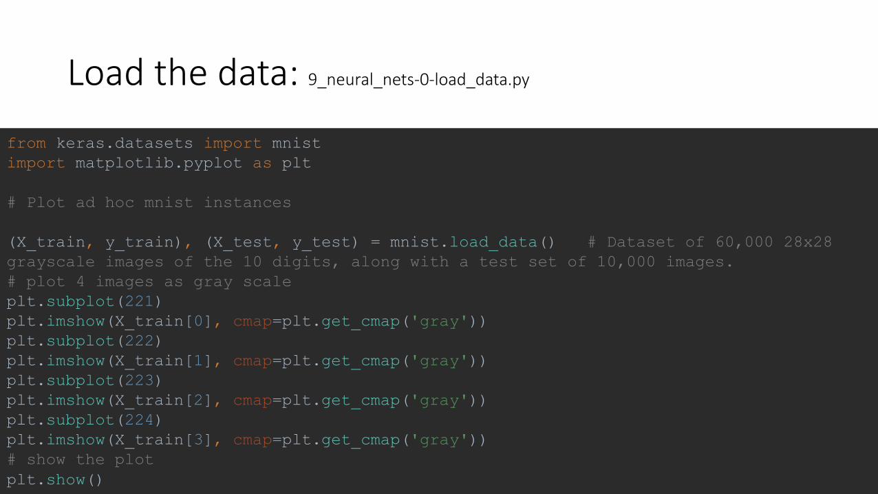
Load the data: 9_neural_nets-0-load_data.py
from keras.datasets import mnist
import matplotlib.pyplot as plt
# Plot ad hoc mnist instances
(X_train, y_train), (X_test, y_test) = mnist.load_data() # Dataset of 60,000 28x28
grayscale images of the 10 digits, along with a test set of 10,000 images.
# plot 4 images as gray scale
plt.subplot(221)
plt.imshow(X_train[0], cmap=plt.get_cmap('gray'))
plt.subplot(222)
plt.imshow(X_train[1], cmap=plt.get_cmap('gray'))
plt.subplot(223)
plt.imshow(X_train[2], cmap=plt.get_cmap('gray'))
plt.subplot(224)
plt.imshow(X_train[3], cmap=plt.get_cmap('gray'))
# show the plot
plt.show()

Prepare data: 9_neural_nets-1-perceptron.py
# fix random seed for reproducibility
seed = 7
numpy.random.seed(seed)
# load data
(X_train, y_train), (X_test, y_test) = mnist.load_data()
# flatten 28*28 images to a 784 vector for each image
num_pixels = X_train.shape[1] * X_train.shape[2]
X_train = X_train.reshape(X_train.shape[0], num_pixels).astype('float32')
X_test = X_test.reshape(X_test.shape[0], num_pixels).astype('float32')
# train-validation split
X_train, X_validation, y_train, y_validation = train_test_split(X_train, y_train, test_size=0.1, random_state=42)
# normalize inputs from 0-255 to 0-1
X_train = X_train / 255
X_test = X_test / 255
# one hot encode outputs
y_train = np_utils.to_categorical(y_train)
y_validation = np_utils.to_categorical(y_validation)
y_test = np_utils.to_categorical(y_test)
num_classes = y_test.shape[1]
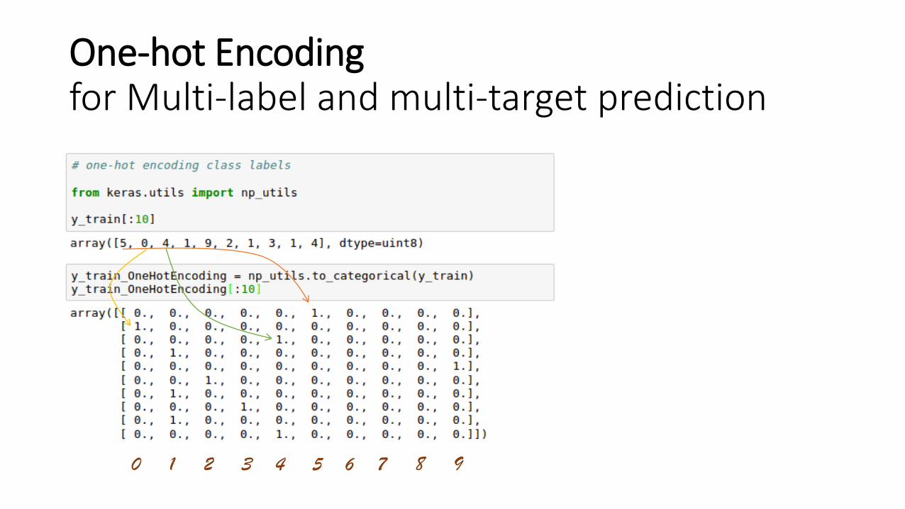
One-hot Encoding for Multi-label and multi-target prediction
0 1 2 3 4 5 6 7 8 9
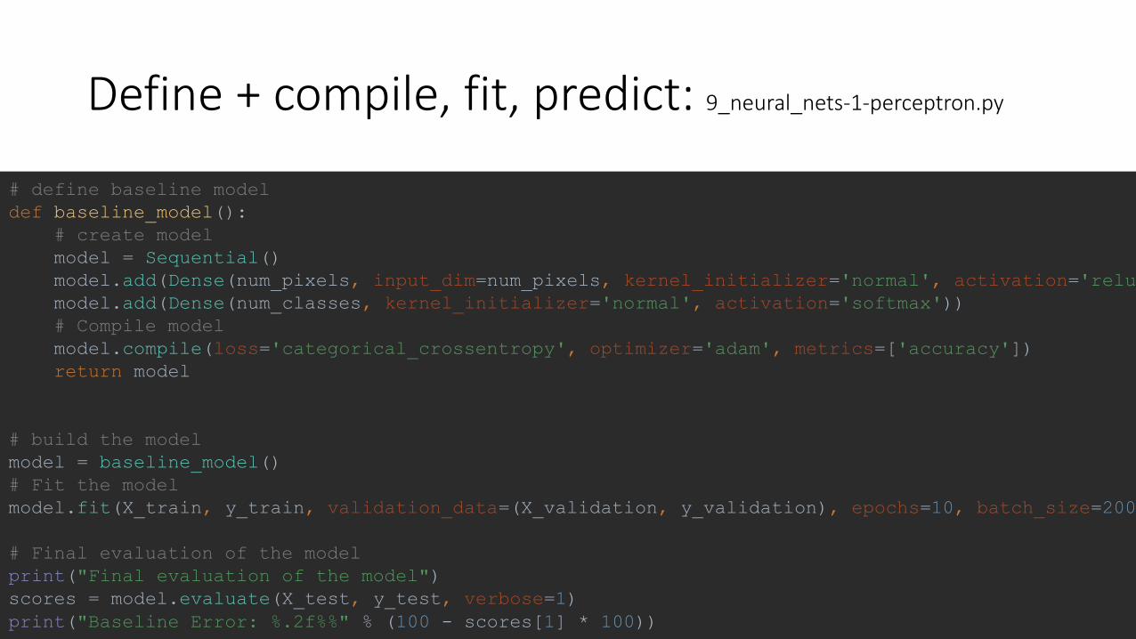
Define + compile, fit, predict: 9_neural_nets-1-perceptron.py
# define baseline model
def baseline_model():
# create model
model = Sequential()
model.add(Dense(num_pixels, input_dim=num_pixels, kernel_initializer='normal', activation='relu'))
model.add(Dense(num_classes, kernel_initializer='normal', activation='softmax'))
# Compile model
model.compile(loss='categorical_crossentropy', optimizer='adam', metrics=['accuracy'])
return model
# build the model
model = baseline_model()
# Fit the model
model.fit(X_train, y_train, validation_data=(X_validation, y_validation), epochs=10, batch_size=200,
# Final evaluation of the model
print("Final evaluation of the model")
scores = model.evaluate(X_test, y_test, verbose=1)
print("Baseline Error: %.2f%%" % (100 - scores[1] * 100))
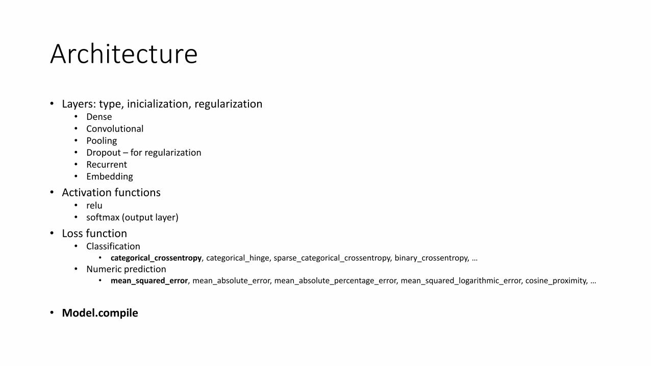
Architecture
• Layers: type, inicialization, regularization• Dense• Convolutional• Pooling• Dropout – for regularization• Recurrent• Embedding
• Activation functions • relu• softmax (output layer)
• Loss function• Classification
• categorical_crossentropy, categorical_hinge, sparse_categorical_crossentropy, binary_crossentropy, …
• Numeric prediction• mean_squared_error, mean_absolute_error, mean_absolute_percentage_error, mean_squared_logarithmic_error, cosine_proximity, …
• Model.compile
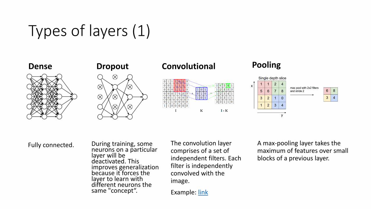
Types of layers (1)
Dense Convolutional
A max-pooling layer takes the maximum of features over small blocks of a previous layer.
Dropout Pooling
Fully connected. During training, some neurons on a particular layer will be deactivated. This improves generalization because it forces the layer to learn with different neurons the same "concept“.
The convolution layer comprises of a set of independent filters. Each filter is independently convolved with the image.
Example: link
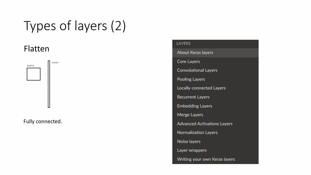
Types of layers (2)
Flatten
Fully connected.
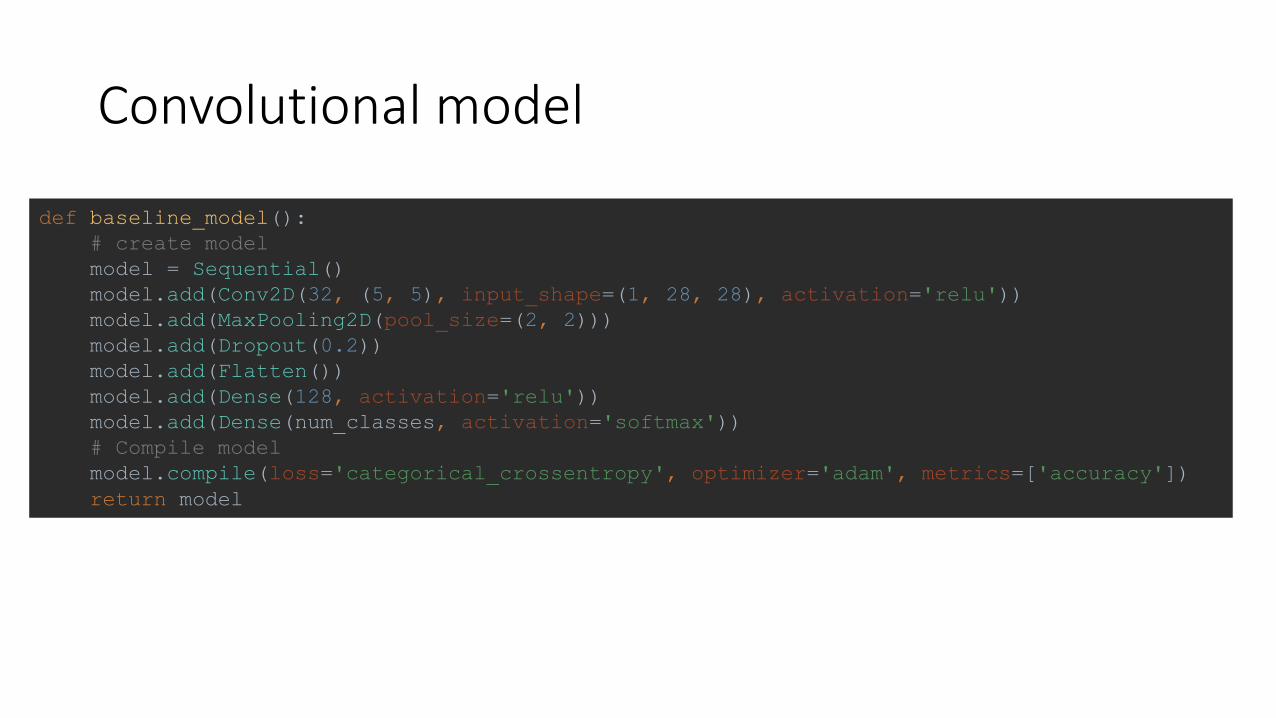
Convolutional model
def baseline_model():
# create model
model = Sequential()
model.add(Conv2D(32, (5, 5), input_shape=(1, 28, 28), activation='relu'))
model.add(MaxPooling2D(pool_size=(2, 2)))
model.add(Dropout(0.2))
model.add(Flatten())
model.add(Dense(128, activation='relu'))
model.add(Dense(num_classes, activation='softmax'))
# Compile model
model.compile(loss='categorical_crossentropy', optimizer='adam', metrics=['accuracy'])
return model
![CNTK: deep learning framework - Nvidiaimages.nvidia.com/events/sc15/pdfs/CNTK-Overview-SC150-Kamanev.pdfmeanFile=$WorkDir$/ImageNet1K_mean.xml ] labels=[ labelDim=1000 ] ] ] Next steps:](https://img.pdfslide.us/doc/110x75/5b3b80847f8b9a26728c9428/cntk-deep-learning-framework-workdirimagenet1kmeanxml-labels-labeldim1000.jpg)


![Benchmarking and Analyzing Deep Neural Network Trainingpekhimenko/Papers/iiswc18-tbd.pdf · frameworks (TensorFlow [8], MXNet [22], CNTK [89]) across different hardware configurations](https://img.pdfslide.us/doc/110x75/5ec680dabfa4d65d8a462ec1/benchmarking-and-analyzing-deep-neural-network-pekhimenkopapersiiswc18-tbdpdf.jpg)
![Comparative Study of Deep Learning Framework in HPC ......2) CNTK The Microsoft Cognitive Toolkit (CNTK) is a unified deep-learning toolkit developed by Microsoft [2]. It provides](https://img.pdfslide.us/doc/110x75/5ec91671233920076327a1d6/comparative-study-of-deep-learning-framework-in-hpc-2-cntk-the-microsoft.jpg)