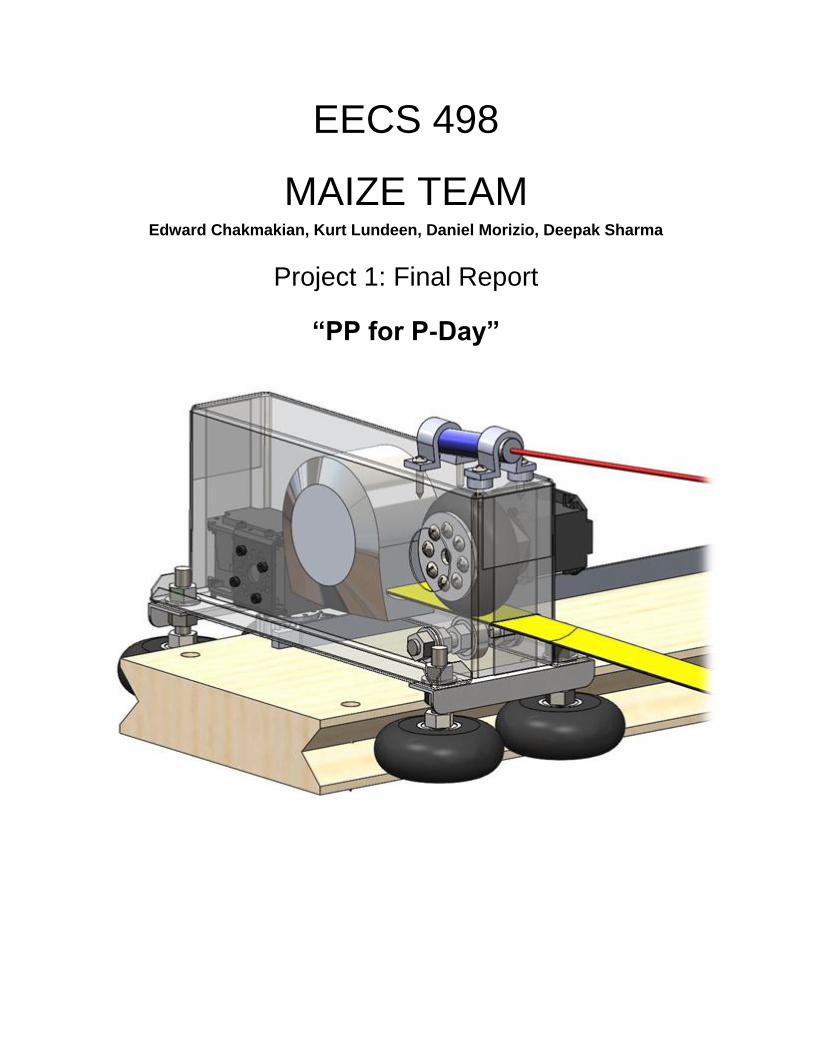
EECS 498

MAIZE TEAM

Edward Chakmakian, Kurt Lundeen, Daniel Morizio, Deepak Sharma

Project 1: Final Report

“PP for P-Day”

CONTENT

1. Background

1.1. Project Introduction

1.2. Equipment Involved

1.2.1. Computer Vision System

1.2.2. Dynamixel RX-64 and EX-106 Servo Motors

1.3. Design brainstorming

1.3.1. Hardware

1.3.1.1. Walker Robot

1.3.1.2. Crane Robot

1.3.1.3. Adaptation to Red teams (2014) Project 0 robot

1.3.1.4. Revolute-Revolute Manipulator Robot

1.3.1.5. Prismatic-Prismatic Robot

1.3.2. Software

2. Implementation

2.1. Initial Concept

2.2. Robot Design and Construction

2.3. Design Considerations

2.3.1. Sources of Error

2.3.2. Re-evaluation and Modifications

2.4. Motion Algorithm

2.4.1. Robot

2.4.2. Manual Controller

2.4.3. Autonomous Controller

3. Expected Performance

3.1. Modelling Software

3.2. Calibration and Modification

4. Results

4.1. P-Day Results

4.2. Observations

5. Discussion

5.1. Discussion of Other Teams

5.2. Reflection on Current Design

5.2.1. Mechanical Design

5.2.2. Software

5.3. Future Modifications

5.3.1. Mechanical Design

5.3.2. Software

6. References

7. Appendix

1. Background

1.1 Project Introduction

The project task is to develop a robot which could reach a sequence of waypoint

tags in a specific order while always pointing a laser mounted on the robot in +y

direction (red line as shown in Figure 1 (Fig. 1)).

Figure 1: Schematic diagram of the 2D tags (grey boxes) and robot with red laser in the

arena.

The details of the project (as discussed in Project 1 Task Specification file [1]) is

mentioned the following four points:

● Trajectory defined by waypoints: The four waypoints enveloped by the corner

tags (as shown in Fig. 1) define the overall path that robot has to take to

complete the task. The location of a waypoint, indicated by tag, is the centroid of

the corners recovered by the vision system. The robot also carries a tag, which

defines the location of the robot. A waypoint is reached when the center of the

robot tag is within the tag diameter of the waypoint tag on the plane of the

waypoint.

● Simulated sensor readings: The project also includes an optional aid provided

by the vision system to help with the navigation of the bot. The vision system

simulates two sensors (cyan and magenta circle markers in Fig. 1). It measures

the perpendicular distance between each sensor and the line segment

connecting previous and next waypoint (tag). If these perpendicular distances fall

outside the segment between the waypoints, or the sensor is too far away from

the line segment, the sensor value is 0.

● Information available to robot: Messages are sent to the robot controller when

the robot tag is observed. This message contains two sets of data. First, the

sensor measurements (as discussed above) in form of a dictionary of key-value

pairs, where keys ‘f’ and ‘b’ indicate the “front” and “back” sensors and have 8-bit

values. Second is the waypoint information; which consists of key ‘w’, which is

part of the aforementioned dictionary, containing a list of waypoints with each

waypoint containing two integers (global x and y coordinates of waypoints). The

waypoints list is sent periodically and when a waypoint is reached. The list keeps

on reducing as the waypoints are reached. Before P-Day trials, coordinates of

four corners of the arena will be given to make safety checks of keeping robot in

the arena. Also, apart from the arena dimensions, another important

measurement consideration is to keep the laser dot projected on the whiteboard

at a distance of at least 25 cm above arena.

● Objective and Pass-Fail criterion: On P-Day, teams will be given 15 minutes to

transverse the waypoints and will be scored on the basis of the RMS (root-of-

mean-of-squares) of the “tracking error”. This error is defined as the difference

between the x-Coordinate of laser dot on screen (whiteboard) and the robot tag’s

projected x-Coordinate (as shown in Fig. 2). After setting the bot in behind the

arena in 1 meter deep area, team can manually drive the bot to the first waypoint.

Upon reaching this waypoint, bot has to automatically navigate through the

remaining three waypoints. To pass the P-Day specification, robot (not just the

tag) has to remain in the arena, robot should reach the final waypoint within 15

minutes and laser should never illuminate in the negative y-direction. In the case

where any of these rules aren’t met, the team will be allowed to manually driving

the bot through remaining waypoints, forfeiting any chances of winning the

competition.

Figure 2: Schematic Representation of “tracking error”.

1.2 Equipment Involved

1.2.1 Computer vision system

To track the arena and robot barcode tags, computer-vision system was provided

that used a Logitech webcam. The software simulated the two aforementioned robot tag

sensors, in addition to mapping arena coordinates and noticing if the robot tag has

reached the next waypoint.

1.2.2 Dynamixel RX-64 and EX-106 Servo Motors

Servo motors were provided along with the python library. These motors allowed

both constant rotation and joint mode operations, where prescribed torque between -1 to

+1 or prescribed angles between -10000 to 10000 could be specified. Maximum of 6

servo motors (a combination of RX-64 and EX motors) were allowed in any suitable

configuration.

1.3 Design Brainstorming

1.3.1 Hardware

Group brainstorming meetings focused on making a design which is efficient and

avoids the usage of complex mechanical structures and mechanisms which could be

interfaced with robust and flexible code. The team came up with 5 designs satisfying the

constraints in the given problem statement. These robot ideas are as follows:

1.3.1.1 Walker Robot

At first, the team came up with an idea of a robot moving on wheels with a

“walker” attached to it. The walker pushes down each time the robot has to turn and

helps in turning of the wheels by lifting them. Walker also mounts the laser on it so that

laser doesn’t change direction each time the robot turns (see Fig. 3). This idea is

inspired from the Blue team’s bot from 2012. The idea was also implemented by Blue

team in this year’s project 1.

Pros and Cons: This bot solves the issue of laser always pointing in the Y-direction.

Also, it discretizes motion in x and y direction only and with good calibration, could lead

to very accurate 90 degree turns. But, on the downside, the robot includes complexity at

both hardware and software ends. Two complex mechanical mechanisms including

rotating wheels and walker are required on the same bot chassis which could hinder

with the laser projection.

Figure 3: Concept design of Walker Robot

1.3.1.2 Crane Robot

This robot uses a slider-linkage mechanism to cover the arena in y-direction by

moving robot in a guided rail. When the robot moves in x-direction, the robot is lifted

using the rope attached to the base of the robot (as shown in Fig. 4). This rope also

helps the bot in pushing and pulling it in y-direction.

Pros and Cons: The robot provides discrete x and y motions running on two different

rails. Also, the bot uses a slider-linkage mechanism which has well-documented

mathematical modeling. But, the bot is bulky in design and may threaten the design

parameters of having less complex design.

Figure 4: Concept design of Crane Robot

1.3.1.3 Adaptation of Red Team’s Project 0 Robot

Red team in project 0 made a robot which could make precise and repeatable

movements and could use a servo controlled turret style laser to adapt to this project.

Pros. and Cons: Fig. 5 shows the robot Red team made for project 0 which has an

advantage that it’s already made but it is susceptible to error accumulation.

Figure 5: Concept design of Adaptation Robot

1.3.1.4 Revolute-Revolute (RR) Manipulator Robot

This robot has two rotating links operated by controlling the joint angles as shown

in Fig. 6.

Pros. and Cons: The bot is able to orient laser quite accurately using synchronized

belt-pulleys as shown in Fig. 7 (side view) and Fig. 8 (top view). But, the bot may require

high torque motor to move the arms. Also, to avoid crossing out of the arena, the bot

may need a robust trajectory planning while reaching waypoints placed anywhere in the

arena.

Figure 6: End effector of R-R robot locating different points in arena (top view)

Figure 7: R-R Robot showing belts and pulley system (side view)

Figure 8: Belt-Pulley system (with constantly upward pointing arrows) of R-R Robot (top view)

1.3.1.5 Prismatic-Prismatic (P-P) Robot

This robot works with two prismatic links moving in both x and y directions. Being

inspired from a video [2] showing the usage of automatically controlled tape measure,

team came up with idea of using the “electric tape measure” to govern the movements

in y-direction. An extension-retraction system shown in Fig. 9. A guiding track made out

of belts, rails or rack and pinion could be used for the movements in x-direction as

shown in Fig. 10 using belt and pulley assembly (as shown in horizontal (x) direction).

Pros and Cons: This robot has a simpler design than that the aforementioned R-R

robot and will require easier to implement control system. But, this bot could be slower

than some of the aforementioned bot designs and will need a better consideration over

measuring the extension of robot tag in y-direction.

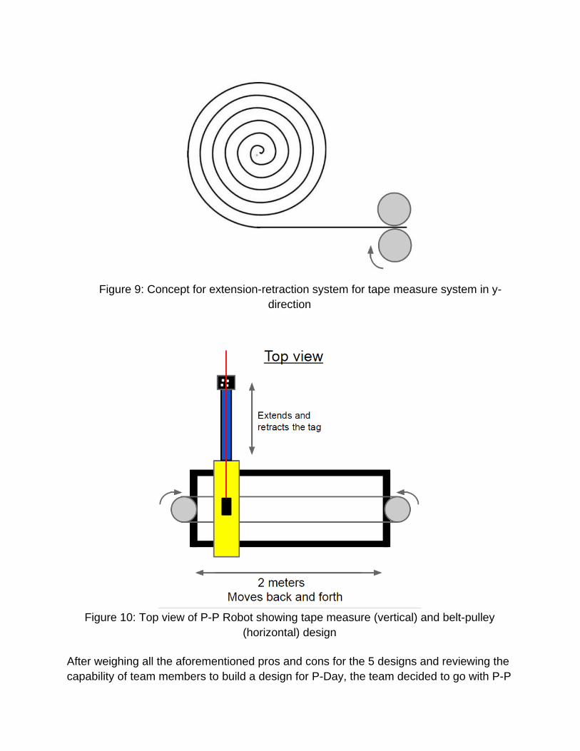
Figure 9: Concept for extension-retraction system for tape measure system in y-

direction

Figure 10: Top view of P-P Robot showing tape measure (vertical) and belt-pulley

(horizontal) design

After weighing all the aforementioned pros and cons for the 5 designs and reviewing the

capability of team members to build a design for P-Day, the team decided to go with P-P

Robot (5th design) and used rack and pinion instead of belt-pulley system for x-direction

motion.

1.3.2 Software

The 1996 paper by Borenstein et al [3] influenced the direction of our software

design. Knowing that the accumulating odometry error of buggy style robots was

unbounded, we quickly settled on a mechanical platform that avoided this movement

style. Initially a revolute-revolute planar manipulator was decided upon and software

development moved forward in this direction. If the team would have settled with this

design, a controller using the inverse kinematics described in Kucuk and Bingul’s Robot

Kinematics [4] would have been implemented in Python to calculate the necessary

servo angles to move to the waypoints. However a mechanical change to a prismatic-

prismatic manipulator changed the course of development.

The initial plan for the software controller was to first implement manual

controller based on the ShaveAndHaircut.py; included in the virtual machine

environment. This would help debug the mechanics of the robot before a final

automated controller was implemented. This manual controller would utilize a Korg MIDI

controller which included sliders, which could be used to fine tune arm speed and

buttons to activate movement.

Finally an autopilot would be implemented which would use the odometry with the

rack and pinion controlling movement in x-direction. A rack and pinion with the

Dynamixel MX-64 motor and its no dead-zone encoder controller was considered

adequately accurate to get our waypoint within the bounds of the target waypoints. This

assumption would need to be tested in system later on and if it fails, additional x-axis

sensors such as the Sharp GP2Y0A21YK0F could be implemented to increase the

accuracy. The flowchart shown in Fig. 11 shows the general outline of the vision for our

robots controller. It is based on the assumption that we would have MX-64 motor

modules and our odometry would be accurate enough to get us within the waypoint

perfectly.

Figure 11. Initial Controller Flowchart

2. Implementation

2.1 Initial Concept

A top view of the initial concept is shown in Fig. 10. The concept was inspired by

the recollection of the existence of electrically-driven tape measures during a

brainstorming discussion. The initial robot concept was drawn with a belt and pulley

system, but it was only meant to represent a generic mechanism for linear translation

along the x- direction.

2.2 Robot Design and Construction

The design process for the Prismatic-Prismatic (PP) Electric Tape Robot began

with a consideration of the robot’s x- and y- movements. The requirement that the robot

be able to reach any point in the arena, combined with the inherent nature of a

prismatic-prismatic manipulator, suggested that the tag should be capable of translating

the entire length of the arena in both the x- and y- directions (see Fig. 12). Such

prismatic motion is often accomplished mechanically by means of rails, guide ways, or

tracks. In some systems like gantry cranes and 3D printing machines, tracks span the

entire workspace and the end effector remains within the confines of the tracks. In other

prismatic systems like cabinet drawers and telescoping cranes, the end effector extends

beyond the limits of the track. In general, spanning tracks over the entire workspace

seemed to offer the benefits of increased position control and mechanical stability.

Figure 12: Competition Arena

The first decision confronting the design was whether to span tracks over the

entire arena, or to extend the robot beyond its tracks. Translations along the x-direction

were considered first. Although the robot is constrained to begin each competition run

inside the setup area, the setup area spans the entire x-dimension of the arena, so it

seemed sensible to span a track along the entire x-dimension of the arena. However,

translations along the y-direction are different. Since the robot is constrained to begin

each run inside the setup area, and since the setup area is outside the span of the

workspace, it follows that the robot must either extend into the arena or deploy a y-

displacement track system into the arena after the start of the run. While deployment of

a track system may have been a surmountable challenge, it seemed to add a level of

complexity to the system in terms of mechanical design and operation. Considering the

time constraints of the project, it was decided to sacrifice position control and

mechanical stability for simplicity in mechanical design and operation. Thus, it was

decided the robot would extend in the y-dimension of the arena, rather than deploying a

track system.

The specifics of the robot’s y-directional extension were considered next. Likely,

the simplest method for extending the robot may be to translate a single rigid member

relative to the main robot. One can imagine a long stick being moved across the robot to

reach long distances. However, such a solution was not pursued because the rigid

member would need to be at least 2 meters long to reach all points in the arena, while

the setup area is only 1 meter deep. Thus, it might be difficult to fit the rigid member in

the setup area at the start of the run, and the member would likely protrude from the

rear of the setup area during the run.

Possibly the next simplest method for extending the robot outward would be to

translate multiple rigid members relative to the robot, and relative to one another, i.e.,

the robot could extend along the y-direction by telescoping. As the setup area is 1 meter

deep and the arena is 2 meters long, the robot would require a minimum of two

telescoping members and one stationary member to reach every point in the arena.

However, the actuation of one member relative to another member, as well as a second

member relative to the first member, in both forward and reverse directions seemed to

present considerable challenges in terms of mechanical design. Thus, the telescoping

solution was not pursued.

Lastly, extending the robot could be accomplished by translating a member

having properties of both rigidity and flexibility. The member could sufficiently resist

compression, bending, and buckling while extending outward, but exhibit those

behaviors when retracted into the setup area. For example, one can think of a tape

measure. A tape measure can be extended out and support its own weight at some

distances, yet can also be retracted and coiled around a spool inside a compact

enclosure. Such a system offers the benefits of being both compact and requiring

actuation of only one member. This was the method selected for extending the robot in

the y direction.

Once it was determined that extension in the y-direction would be accomplished

by a member possessing both rigidity and flexibility, a further investigation of that

mechanism was in order. As previously mentioned, a tape measure is capable of

exhibiting both rigidity and flexibility by changing its cross sectional shape. The tape can

be thought of as a spring. In fact, one material commonly used to make tape measures

is spring steel. The tape is pre-stressed to form a cupped shape when relaxed, but can

be flattened when rolled against a flat spool. Due to the properties of spring material, the

tape will return to a cupped shape after leaving the spool. A comparison of a cupped

tape cross section versus a flattened tape cross section is shown in Fig. 12, where the

images represent the tape in extension from the robot. It can be seen that, in general,

the cupped cross-sectional area has shifted away from the neutral axis. In other words,

each infinitesimal area of the cross section has a greater y-displacement from the

neutral axis, and thus the squared sum of infinitesimal area centroid y-displacements

has increased. More concisely, the second moment of area, 𝐼, has increased (see the

equation below).

𝐼𝑥𝑥 = ∫ ∫ 𝑦2𝑑𝑥 𝑑𝑦𝐴

Material stress due to bending is related to the inverse of the second moment of

area, 𝐼. Thus, the internal stresses in the tape are less in the cupped shape, and the

material is better able to support the load of its own weight (with some deflection).

Figure 12: Cross Sections and Side Views of Extended Members

Although a tape measure is known to exhibit the desired characteristics of rigid

extension and flexible storage, a brainstorming of alternatives led to a counterpart

foamcore concept. In the foamcore concept, a piece of ½” or 1” thick foamcore is cut

into a beam. Then, transverse slits are cut through the foamcore at a fixed interval along

the length of the beam, leaving the upper skin intact (see Fig. 13). When the foamcore is

rolled on a spool, the slits open, and the foamcore beam bends into an arc. When the

foamcore is extended, the slits close, and the lower portions of the foamcore compress

against one another. The foamcore concept works in a similar manner to the tape (see

Fig. 12). If the foamcore is thick, its second moment of area will be large, its internal

stresses will be low enough to resist crushing or tearing, and the foamcore will stand

horizontally (with some deflection). The foamcore might be actuated by driving the spool

itself, or by driving the foamcore with smooth or toothed rollers. The foamcore concept

seemed like a viable solution, but was not pursued due to lack of familiarity with the

material’s characteristics and concerns about bulkiness.

Fig. 13: Foamcore Beam Concept

Having decided that a tape measure would be used for y-extension, actuation of

the tape was considered next. Brainstorming led to three primary options for actuating

the tape: drive the tape using toothed rollers, drive the spool directly, and drive the tape

using smooth rollers. Driving the tape using toothed rollers offers the benefits of

negligible accumulated slip and tracking error, but may require making numerous

precision cuts in the tape material. Additionally, such cuts may have the undesirable

effect of increasing the tape’s deflection. Driving the spool directly offers the benefits of

negligible accumulated slip and tracking error. However, in order for the system to

function properly, the tape measure would need a smooth outer track upon which to

slide as it is uncoiling from the spool. One can imagine attempting to drive a tape by

rotating a spool. When the spool is rotated backward, the tape is pulled firmly against

the spool, but when the spool is rotated forward, the tape may have a tendency to uncoil

itself from the spool. Thus, rotating the spool forward does not necessarily produce

forward motion of the tape out of the enclosure, but rather, might cause unspooling of

the tape inside the enclosure. The spool itself can be thought of as an inner track to

guide the tape as it is being drawn inside the enclosure, but tape measures, in general,

do not possess an outer track to guide the tape as it is being pushed out of the

enclosure. This is due to the fact that tapes are generally not pushed out of the

enclosure, but pulled out. Attempts were made to create a smooth outer track to allow

for a spool-driven system, but were unsuccessful. Based on observations, it seemed

likely that such an outer track could be successfully developed, if given more time. Thus,

it was decided the tape itself would be driven by smooth rollers. Despite the fact that

smooth rollers were expected to produce slip and tracking errors, they offered simplicity

in terms of mechanical design and fabrication.

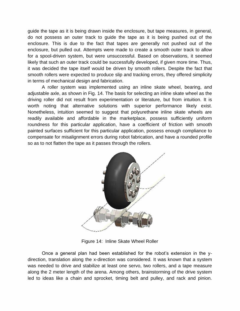
A roller system was implemented using an inline skate wheel, bearing, and

adjustable axle, as shown in Fig. 14. The basis for selecting an inline skate wheel as the

driving roller did not result from experimentation or literature, but from intuition. It is

worth noting that alternative solutions with superior performance likely exist.

Nonetheless, intuition seemed to suggest that polyurethane inline skate wheels are

readily available and affordable in the marketplace, possess sufficiently uniform

roundness for this particular application, have a coefficient of friction with smooth

painted surfaces sufficient for this particular application, possess enough compliance to

compensate for misalignment errors during robot fabrication, and have a rounded profile

so as to not flatten the tape as it passes through the rollers.

Figure 14: Inline Skate Wheel Roller

Once a general plan had been established for the robot’s extension in the y-

direction, translation along the x-direction was considered. It was known that a system

was needed to drive and stabilize at least one servo, two rollers, and a tape measure

along the 2 meter length of the arena. Among others, brainstorming of the drive system

led to ideas like a chain and sprocket, timing belt and pulley, and rack and pinion.

Although all three systems seemed equally suitable for driving the robot along the 2

meter span, a search of sizes and pricing suggested that a nylon rack and pinion system

would likely be the most economical solution.

Not only was it important to consider the mechanism for driving the robot’s

translation along the x-direction, but also stabilizing such movements. For the case of

this particular robot, it was expected that control the robot’s Euler angles would be

critical to the robot’s performance due to the distance of the laser from the screen. For

example, with the tag fully retracted, the tag and laser pointer could be approximated as

being at the same location, roughly 3 meters from the projection screen. In such a case,

a 1 degree perturbation in the robot’s yaw angle could produce roughly a 5 centimeter

discrepancy between the tag’s x-location and the projected laser dot’s x-location.

Similarly, with the tag fully extended (2 meters from the robot), a perturbation in yaw

angle could initiate oscillations in the tape. The tape’s oscillations could potentially

continue after the main robot and laser have come to rest, thereby accumulating error

from discrepancies between the tag’s x-location and the projected laser dot’s x-location

until the oscillations dampen out.

The mechanism selected for achieving such stabilization was a track and loaded

roller system. By preloading the rollers against the track, especially with a viscoelastic

material, the robot is equipped with some ability to reject disturbances from such

sources as track irregularities, roller irregularities, friction between the tape and the

ground, and resistance between the tag and air. Similar to passive automobile

suspension systems, which consist of a spring and a damper, viscoelastic materials

naturally exhibit the properties of a spring and a damper. Thus, polyurethane inline

skate wheels were selected for the track rollers due to their perceived market availability

and affordability, uniform roundness, viscoelastic material properties, and rounded

profile. The reason for seeking a rounded profile was to provide the robot with

multidirectional support. As can be seen in Fig. 15, the combination of a rounded profile

roller and a v-grooved track allows for directional control of the contact forces. The

multidirectional, preloaded forces statically load the robot’s body in all degrees of

freedom (y, z, yaw, pitch, and roll) except along the x-direction. These forces, along with

the damping properties of the rollers, act to support the weight of the robot, reduce

impulse forces between the rollers and track that might otherwise occur if the rollers

were not statically loaded, and help to reject disturbances to the system.

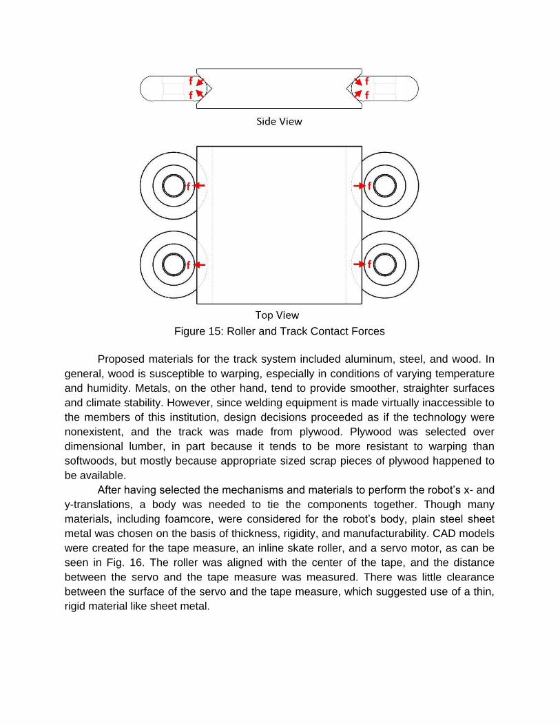
Figure 15: Roller and Track Contact Forces

Proposed materials for the track system included aluminum, steel, and wood. In

general, wood is susceptible to warping, especially in conditions of varying temperature

and humidity. Metals, on the other hand, tend to provide smoother, straighter surfaces

and climate stability. However, since welding equipment is made virtually inaccessible to

the members of this institution, design decisions proceeded as if the technology were

nonexistent, and the track was made from plywood. Plywood was selected over

dimensional lumber, in part because it tends to be more resistant to warping than

softwoods, but mostly because appropriate sized scrap pieces of plywood happened to

be available.

After having selected the mechanisms and materials to perform the robot’s x- and

y-translations, a body was needed to tie the components together. Though many

materials, including foamcore, were considered for the robot’s body, plain steel sheet

metal was chosen on the basis of thickness, rigidity, and manufacturability. CAD models

were created for the tape measure, an inline skate roller, and a servo motor, as can be

seen in Fig. 16. The roller was aligned with the center of the tape, and the distance

between the servo and the tape measure was measured. There was little clearance

between the surface of the servo and the tape measure, which suggested use of a thin,

rigid material like sheet metal.

Figure 16: Clearance between Tape Measure and Servo Influences Material Selection

Another design concern was the potential for tracking error caused by

misalignment of the roller. It was anticipated that a high force would be required

between the roller and the tape to minimize tape slip, but that such a force might

inadvertently bend the body of the robot. As can be seen in Fig. 17 where the body of

the robot is represented by a green line, bending of the body can result in misalignment

of the roller, and therefore tracking error of the tape. Thus, rigidity was also an important

criteria for selection of the body material. Additionally, sheet metal was selected

because it was a material with which members of the team were familiar.

Figure 17: Potential for Body Bending to Produce Tracking Errors

Lastly, a guide way was incorporated in the design as a mechanism for limiting

the accumulation of tape tracking error. If the roller were to push the tape to the left or

right, the tape would track to that side until contacting the guide way. Upon contact,

forces exerted on the tape from the guide way would restrict the tape from tracking

further. Said another way, the slot’s edges would act to constrain the transverse motion

of the tape. The guide way was formed by cutting a rectangular slot in the robot body, as

shown in Fig. 18.

Figure 18: Tape Guide way to Limit Accumulation of Tape Tracking Error

More details regarding the specific dimensions, materials, hardware, costs, CAD

files, and manufacturing processes used to make the Prismatic-Prismatic (PP) Electric

Tape Robot can be found in the project construction document [5].

2.3 Design Considerations

2.3.1 Sources of Error

We identified three main potential sources of error for our robot: camera

projection, tape measure angle, and y-axis slip. Of the three errors, we concluded that y-

axis slip error caused by extending and retracting our tag would be the most problematic

for our design. Below is a more in depth description and our thoughts on each of these

errors.

Camera projection error is the error caused by having the tag off of the ground at

a certain height. Fig. 19 shows the physical set up of the arena how we can

conceptualize the projection error.

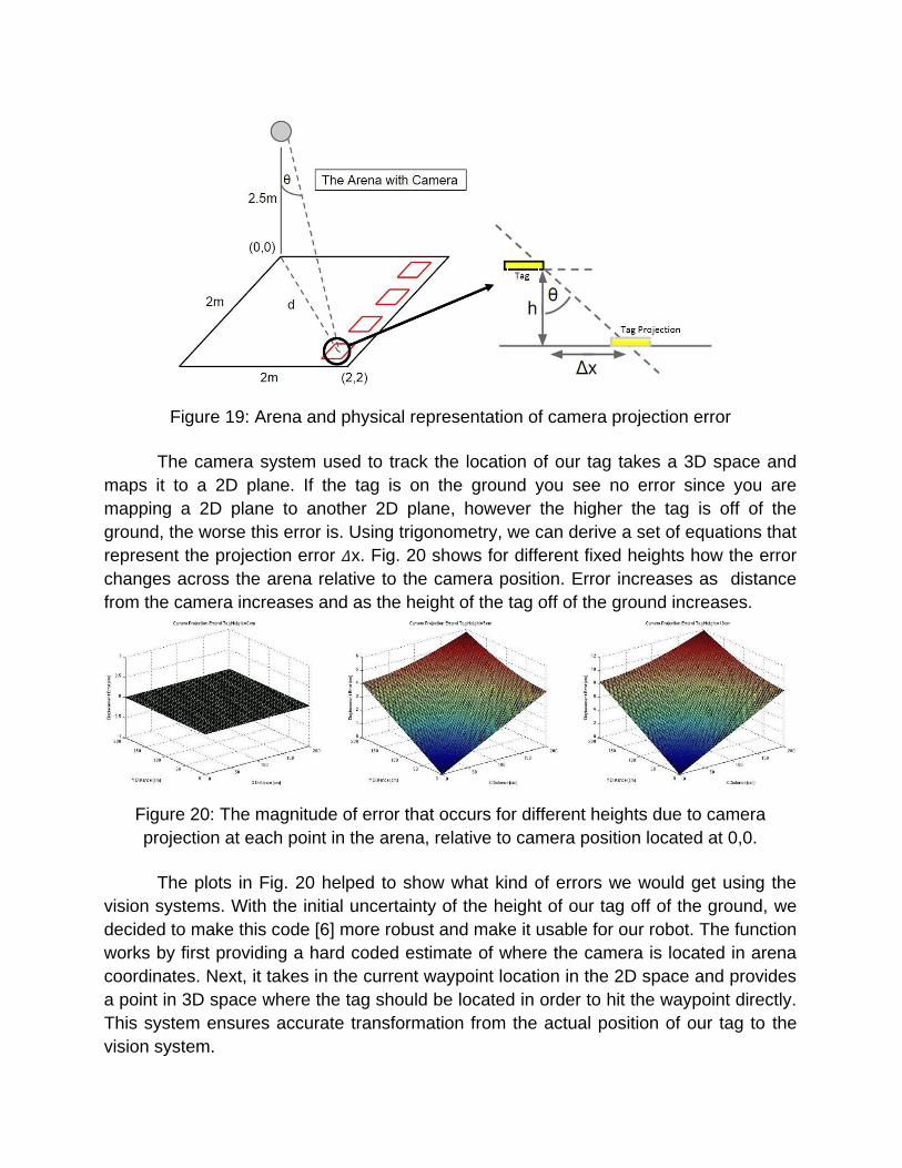
Figure 19: Arena and physical representation of camera projection error

The camera system used to track the location of our tag takes a 3D space and

maps it to a 2D plane. If the tag is on the ground you see no error since you are

mapping a 2D plane to another 2D plane, however the higher the tag is off of the

ground, the worse this error is. Using trigonometry, we can derive a set of equations that

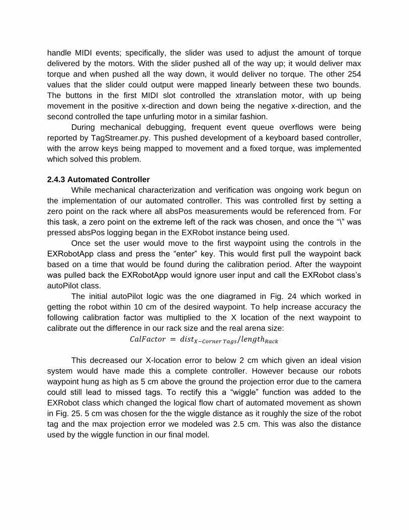
represent the projection error 𝛥x. Fig. 20 shows for different fixed heights how the error

changes across the arena relative to the camera position. Error increases as distance

from the camera increases and as the height of the tag off of the ground increases.

Figure 20: The magnitude of error that occurs for different heights due to camera

projection at each point in the arena, relative to camera position located at 0,0.

The plots in Fig. 20 helped to show what kind of errors we would get using the

vision systems. With the initial uncertainty of the height of our tag off of the ground, we

decided to make this code [6] more robust and make it usable for our robot. The function

works by first providing a hard coded estimate of where the camera is located in arena

coordinates. Next, it takes in the current waypoint location in the 2D space and provides

a point in 3D space where the tag should be located in order to hit the waypoint directly.

This system ensures accurate transformation from the actual position of our tag to the

vision system.

Tape measure angle error is caused by the potential of our tape to extend at

some angle theta away from our desired path; our desired path is parallel with the laser

which is shown in Fig. 21. This deflection in theta could be caused by misalignment or a

force on the side of the tape measure. To gauge how bad of a problem this would be for

our robot, we applied a force to the tape while it was extended; we measured a

maximum deflection angle 𝜃=10°. Fig. 22 shows error with respect to the distance our

tape is extended and the angle 𝜃. It is easily seen that as both theta and the extended

distance increase, the error is very large.

Figure 21: Tape measure angle error caused by misalignment or force on the side of the

tape measure

Figure 22: Error of the tape measure as it extends out at different angles

This error can be related to the acceleration of the base in x-direction. Using the

first principles, this arrangement could be related to an accelerated pendulum where the

tape acts like a pendulum. Two forces (given air drag is assumed to be zero) acting on

the end of the hanging tape are surface friction (F) and tension force (T) caused by tape.

For an acceleration of “a”, there’s a deflection in tape by an angle theta when the end of

the tape moves with a velocity “v” (as shown in Fig. 23).

Figure 23: Schematic representation of accelerating robot (base) and deflecting tape

This system of forces could be resolved in x and y direction as follows:

X- Direction: 𝑇. 𝑐𝑜𝑠(𝜃) − 𝐹. 𝑠𝑖𝑛(𝜃) = 𝑚.𝑣2

𝐿

Y- Direction:𝑇. 𝑠𝑖𝑛𝜃) + 𝐹. 𝑐𝑜𝑠(𝜃) = 𝑚. 𝑎

where,

F= K.(Normal from ground)= K.m.g ;

K= Coefficient of rolling friction, m=mass of the end (clip) of measuring tape, g=gravitational force constant.

These equations give x-acceleration in terms of deflection angle error 𝜃 as:

𝑎 =𝑣2. 𝑡𝑎𝑛 (𝜃)

𝐿+ 𝐾. 𝑔. 𝑠𝑒𝑐( 𝜃)

Using this equation, for a given value of 𝜃, appropriate value of acceleration could be

obtained.

Y-axis slip error is caused by the slipping of the roller on the tape as it extends or

retracts. This is a problem because if there is a little bit of slippage, it goes unaccounted

for because there is no way to track it. This error is even more dangerous because it

will accumulate throughout the run. There is no way to accurately model y-axis slip error

for our system because it is based solely off physical design and performance of the

system. However, it is easy to conceptualize how to reduce this slippage; we can

increase the friction between the roller and the tap. This could be done by adding a

material with a high friction coefficient or by providing a large upward force on the tape.

2.3.2 Re-evaluations and Modifications

After looking at our potential errors and where our robot could fail, we made

several conclusions. The first, our robot’s tag should remain as close to the ground as

possible. Large errors in both finding the waypoints and laser tracking make us shy

away from having a tag high off the ground. Instead of angling our tape measure up in

the air so that when fully extend it does not hit the ground, we extend our tape out

straight with no angle compensation and allow it to hit the ground. The tag will hit the

ground when the tape is extended at a distance of approximately one meter. Once it hits

the ground, it will slide on a furniture slider that is placed at the end of the tape. After

looking at Fig. 20 and taking into account the low heights of our tag, the camera

projection error seems negligible. Also with this modification, it limits our movement in

the x-direction as the tape will be touching the ground producing friction force. Similar to

Fig. 21, the tape will experience some amount of angular deflection. Since the tape Is

subject to deflect up to 10° and causing a large error, we found it best not to translate in

the x-direction while the end of the tape was touching the ground.

The second conclusion we made is that a guardrail for the tape measure should

be in place to ensure the extension and retraction of the tape was inline with the laser.

Looking at Fig. 22, it is clear that if we can limit angle 𝜃 to less that 1.5°, the error will be

reduced for most of the points in the arena. But during testing, it was observed that even

with the guardrail in place, the tape still wobbled while translating in the x-direction as it

touched the ground. This leaves us with only one option of retracting the tape and tag in

the y-direction, before each x-direction movement from one tag to another. With this

being said, we no longer have to take into the x-acceleration error since we will be

moving with our tag fully retracted. Overall, this modification simplifies the movement of

our robot.

The last conclusion we made was that we would not be able to track the y-

position of our tag accurately if there is slip between the roller and the tape. If we tried to

match the tag position with the encoder in the motor and slip occurred, the encoder

value would not match up with tag position. Over time, this error would accumulate and

the tag would not be able to hit the waypoints and potentially go out of bounds. To

compensate for this, our plan is to fully extend our tag to the edge of the arena and then

retract it back to its original location based off of a manual time calibration. This

calibration will help to alleviate the uncertainties associated with the tape extension.

2.4 Motion Algorithm

2.4.1 Robot

Inside of Robot.py there are two implementations of a robot included. The first

class named Robot was designed under the assumption that we would be using MX-64

motors. These motors would be populated by the Cluster command in the logical.py

module and passed into the Robot instance. The original implementation of this robot

was designed with guiding idea that the rack which our robot rode on could be broken

up into integer N rotation chunks and then its location could be fine tuned using the no

deadzone encoder in the MX-64 motor controller. This was chosen as due to the

diameter of our pinion being 3.18 cm which led to the full rotation x-translation shown

below:

𝑑𝑒𝑛𝑐𝑜𝑑𝑒𝑟 ∗ 𝜋 = 9.99 𝑐𝑚

This nicely segmented the the arena into 20 equal chunks. Movement was

facilitated by the moveNRotationsForward and moveNRotationsBackward functions

inside the robot. These would move the robot approximately 10cm to the right or left

respectively and update the robots Xrotations variable by the amount of rotations

moved. Fine movement was handled by the move2EncoderPos and the

move2EncoderPosBack functions which when given an encoder position would move

the robot to within 1° or 0.028 of the desired location. Once the use of our two MX-64

modules was made impossible due to failure, development of this class was halted.

The second class in Robot.py named EXRobot was the class used for our robot

once we had made the switch to EX-106 motor modules and the one used in final

competetion. The deadzone in these modules was large and thus could not be used

reliably with the code developed for the MX-64 modules. The decision was made to

instead configure the EX-106 modules for multi-turn mode which reported encoder

positions from -13000 to 390000 in units of hundredths of a degree. Given this fact, an

incrementPosRegister was developed which, during movement would increment the

absPos instance variable to keep track of absolute position of the robot on the rack.

Next a function called calcTargetPos was developed to calculate the

corresponding absPos needed to line the robot tag with the next waypoint tag. This

value was stored in the targetPos member variable. This function along with checkPast

were the two functions that facilitated the logic of movement in the autopilot. The

function checkPast would return false unless absPos was greater or less than the

targetPos for forward and backward movement respectively.

The last base EXRobot function was the unfurl function. This facilitated the

expelling of the tape measure and its subsequent retraction. It based its timing using the

time library in Python, which was deemed sufficient as the only alternative was to

implement another sensor for control.

2.4.2 Manual Controller

The slider and buttons of the Korg MIDI controller made it easy to create a

manual controller that offered our team the ability to test our mechanical platform easily.

Our implementation is contatined in TagStreamer.py and used a joyApp subclass to

handle MIDI events; specifically, the slider was used to adjust the amount of torque

delivered by the motors. With the slider pushed all of the way up; it would deliver max

torque and when pushed all the way down, it would deliver no torque. The other 254

values that the slider could output were mapped linearly between these two bounds.

The buttons in the first MIDI slot controlled the xtranslation motor, with up being

movement in the positive x-direction and down being the negative x-direction, and the

second controlled the tape unfurling motor in a similar fashion.

During mechanical debugging, frequent event queue overflows were being

reported by TagStreamer.py. This pushed development of a keyboard based controller,

with the arrow keys being mapped to movement and a fixed torque, was implemented

which solved this problem.

2.4.3 Automated Controller

While mechanical characterization and verification was ongoing work begun on

the implementation of our automated controller. This was controlled first by setting a

zero point on the rack where all absPos measurements would be referenced from. For

this task, a zero point on the extreme left of the rack was chosen, and once the “\” was

pressed absPos logging began in the EXRobot instance being used.

Once set the user would move to the first waypoint using the controls in the

EXRobotApp class and press the “enter” key. This would first pull the waypoint back

based on a time that would be found during the calibration period. After the waypoint

was pulled back the EXRobotApp would ignore user input and call the EXRobot class’s

autoPilot class.

The initial autoPilot logic was the one diagramed in Fig. 24 which worked in

getting the robot within 10 cm of the desired waypoint. To help increase accuracy the

following calibration factor was multiplied to the X location of the next waypoint to

calibrate out the difference in our rack size and the real arena size:

𝐶𝑎𝑙𝐹𝑎𝑐𝑡𝑜𝑟 = 𝑑𝑖𝑠𝑡𝑋−𝐶𝑜𝑟𝑛𝑒𝑟 𝑇𝑎𝑔𝑠/𝑙𝑒𝑛𝑔𝑡ℎ𝑅𝑎𝑐𝑘

This decreased our X-location error to below 2 cm which given an ideal vision

system would have made this a complete controller. However because our robots

waypoint hung as high as 5 cm above the ground the projection error due to the camera

could still lead to missed tags. To rectify this a “wiggle” function was added to the

EXRobot class which changed the logical flow chart of automated movement as shown

in Fig. 25. 5 cm was chosen for the the wiggle distance as it roughly the size of the robot

tag and the max projection error we modeled was 2.5 cm. This was also the distance

used by the wiggle function in our final model.

Figure 24: Initial Controller Flowchart

Figure 25: Final Controller Flowchart

Wherever set_torque commands were sent to the two motors a value of .5 input.

This was decided because we verified that this was a torque high enough to ensure

movement both directions without being too fast for the camera system.

3. Expected Performance

3.1 Modeling Software

The modeling code for our robot was stored in simTagStreamer.py, robotSim.py,

robotFunctions.py and plotter.py. simTagStreamer.py holds both the manual controls

for the robot along with the mechanism by which the robots postion is reported to

waypointServer.py in the TestRobot class. The manual control was implemented with

the left and right arrow keys handling negative and positive x-axis translation and the up

and down arrow keys handling positive and negative y-axis translation. Two other

controls were also implemented. The first being a save function which is controlled by

the ‘s’ key and saves a log of the laser and tag position for plotting. The other control is

the autopilot controlled by the ‘a’ key. Once pressed the robot assumes full control of its

motions.

The error modeling is implemented in the robotFuncitons.py which includes

functions that handle the three sources of error: the tape being expelled at an angle, the

error induced by the camera and slip on the tape and rack and pinion. The function

tapeAngleError returns an array of the x-axis and y-Axis error induced by the measuring

tape being expelled at an angle relative to the laser pointer. These values are governed

by the following equations:

𝑥𝑒𝑟𝑟𝑜𝑟 = 𝑡𝑎𝑝𝑒𝐿𝑒𝑛𝑔𝑡ℎ ∗ 𝑠𝑖𝑛(𝜃𝑒𝑟𝑟𝑜𝑟)

𝑦𝑒𝑟𝑟𝑜𝑟 = 𝑡𝑎𝑝𝑒𝐿𝑒𝑛𝑔𝑡ℎ − 𝑡𝑎𝑝𝑒𝐿𝑒𝑛𝑔𝑡ℎ ∗ 𝑐𝑜𝑠(𝜃𝑒𝑟𝑟𝑜𝑟)

The function cameraProjectionError implements the error caused by the camera

not being positioned at the same x and y location of our robot. This error is implemented

as shown in the previous section and has a controllable height parameter referring to

the height of our robot’s tag off the ground.

Finally the slipError function takes in a given movement distance and returns a

movement distance that is subject to some slip in the actuation. We modeled slip as a

simple coefficient referring to the percentage of motor rotation that has no effect on

movement. As an example a movement distance of 1m and a slipCoef of 0.1 would be

returned as 99cm

The functional logic for our robot is held in robotSim.py, specifically in the

ppRobot class. This includes the horizTranslate and vertTranslate functions which

facilitate a horizontal or vertical translation respectively based on some input distance. A

save function is also implemented which pickles (a form of data serialization) a log of

laser location and waypoint location data for later plotting. Finally the autopilot and

wiggle functions handle autonomous motion using the same program flow as shown in

Fig. 25.

To get a better idea of robot performance relative to the task a plotting tool,

plotter.py, was also developed which unpickles the laser and waypoint location saved in

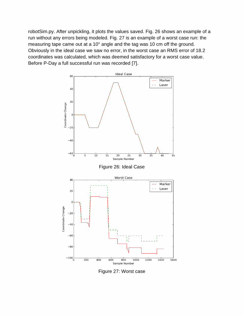
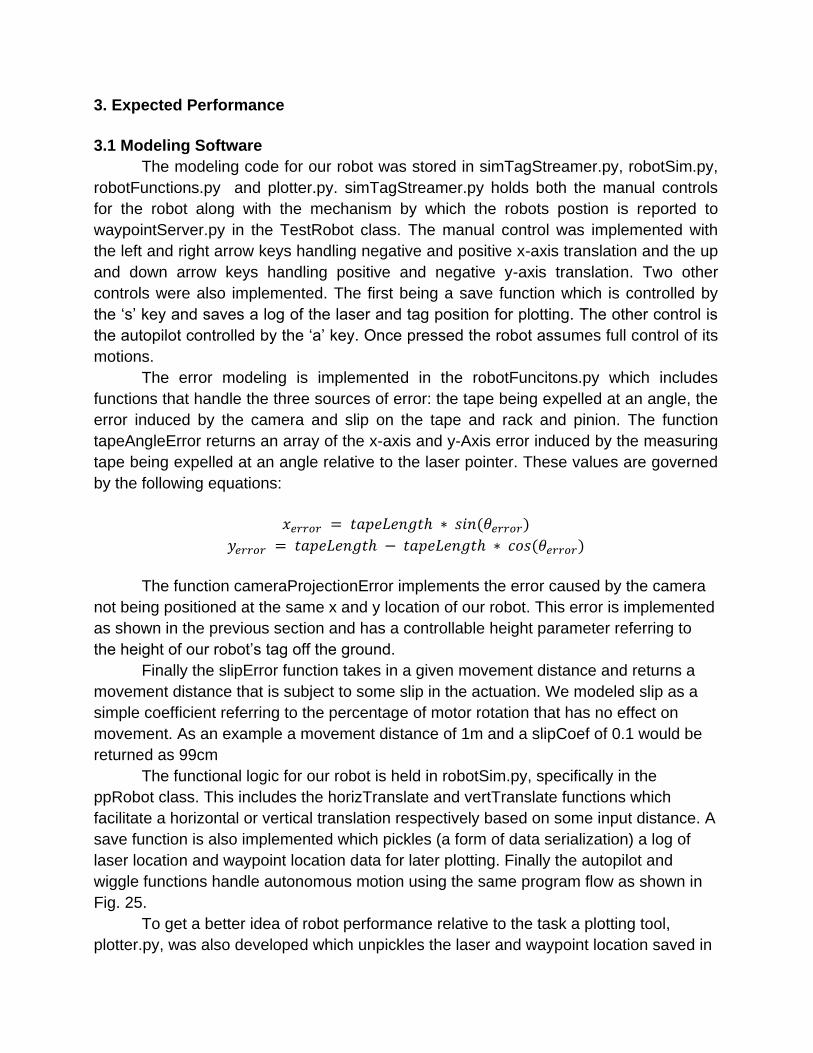
robotSim.py. After unpickling, it plots the values saved. Fig. 26 shows an example of a

run without any errors being modeled. Fig. 27 is an example of a worst case run: the

measuring tape came out at a 10° angle and the tag was 10 cm off the ground.

Obviously in the ideal case we saw no error, in the worst case an RMS error of 18.2

coordinates was calculated, which was deemed satisfactory for a worst case value.

Before P-Day a full successful run was recorded [7].

Figure 26: Ideal Case

Figure 27: Worst case

3.2 Calibration and Verification

3.2.1 Laser Calibration

In order to verify that our robot’s laser system, we used a long exposure camera.

During the test, we moved our robot from one end of the track to the other end and then

back to the original position, thus covering the full range of x-translation. Fig. 28 shows

that our laser tracks a horizontal line during the test. This is exactly what we expect with

our robot since our laser only moves along the x-axis. This laser tracking provides us

with a visual representation of what the camera system will see during P-Day.

Figure 28: Long Exposure Picture of Real Time Laser Tracking

3.2.2 Tape Angle Validation

In testing our measuring tape before its installation inside of the housing we

measured a maximum deflection angle of 10 degrees. This would lead to a maximum

tag to laser x-location error of 35 cm. This was deemed unacceptable so in the final

mechanical design a small output window 3 cms after the output of the measuring tape

was added to help keep the tape straight. Fig. 29 shows two images of the tape being

extended from the same location and an overlay showing the output angle. The output

angle is clearly smaller than the maximum of 10 degrees allowed for in our model. We

concluded that this error is negligible.

Figure 29: Tape Angle Validation

(The red line represents the initial axis of the measuring tape before extending it to a

length of 2 meters. After full extension, we can see that the red line deviates slightly

from the center of measuring tape. We found this error be negligible.)

3.2.3 X-Movement Slip Verification

Due to its rack and pinion design it was assumed before testing that the X-

translation would be very resistant to slip. This was validated using Fig. 30 below that

shows two images of the robot moving 5 rotations to the right and back taken from the

same position. No slip was observed.

Figure 30: x-translation Slip Validation

The red box represents the initial position of our tag. After moving 5 rotations and

coming back to the original position, we can see that the error is minimal.

3.2.4 Tape Extension Calibration

To ensure our robot would not be disqualified we calibrated the tape unfurling by

measuring the time it took to fully extend the tape and the time it took to completely

detract it. This measurement was required in both directions because we noticed after

repeated usage that the retracting slip was larger than the extending. In the end, values

of 10.5 seconds for unfurling and 12 seconds for retracting were decided upon.

3.2.5 X-Translation Calibration

The X-length of the arena could be variable and our rack is of constant length.

We established a scale factor by using the following expression:

(x-length of the arena)/(x-length of our rack)

This factor helps us to achieve the correct x-position on our rack in relation to the arena

coordinates.

4. Results

4.1 P-Day Results

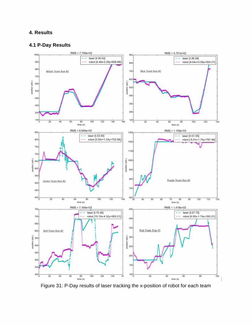
Figure 31: P-Day results of laser tracking the x-position of robot for each team

On P-Day, each team was allowed two attempts to complete the course. For the

second attempt, the arena was modified and one waypoint was moved. Many teams

had issues on the first run and decided to run their robots manually to ensure course

completion. However, during a manual run, scores did not count toward the competition.

Fig. 31 shows each teams results during the second run of the competition.

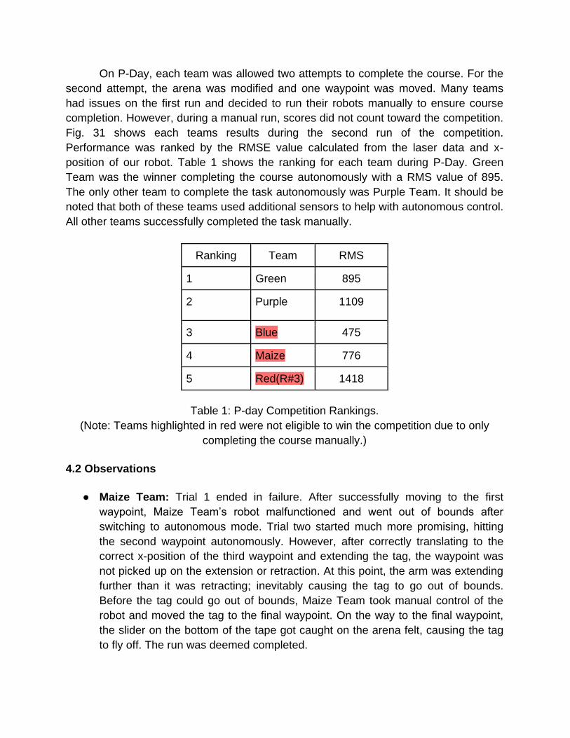
Performance was ranked by the RMSE value calculated from the laser data and x-

position of our robot. Table 1 shows the ranking for each team during P-Day. Green

Team was the winner completing the course autonomously with a RMS value of 895.

The only other team to complete the task autonomously was Purple Team. It should be

noted that both of these teams used additional sensors to help with autonomous control.

All other teams successfully completed the task manually.

Ranking Team RMS

1 Green 895

2 Purple 1109

3 Blue 475

4 Maize 776

5 Red(R#3) 1418

Table 1: P-day Competition Rankings.

(Note: Teams highlighted in red were not eligible to win the competition due to only

completing the course manually.)

4.2 Observations

● Maize Team: Trial 1 ended in failure. After successfully moving to the first

waypoint, Maize Team’s robot malfunctioned and went out of bounds after

switching to autonomous mode. Trial two started much more promising, hitting

the second waypoint autonomously. However, after correctly translating to the

correct x-position of the third waypoint and extending the tag, the waypoint was

not picked up on the extension or retraction. At this point, the arm was extending

further than it was retracting; inevitably causing the tag to go out of bounds.

Before the tag could go out of bounds, Maize Team took manual control of the

robot and moved the tag to the final waypoint. On the way to the final waypoint,

the slider on the bottom of the tape got caught on the arena felt, causing the tag

to fly off. The run was deemed completed.

● Green Team: In trial 1, Green Team successfully navigated to the second

waypoint autonomously. However, an error in their code prevented them from

finishing the course autonomously and they were forced to manually finish the

run. During trial 2, they successfully completed the course autonomously. The

laser looked a little jumpy during the run, but based on Fig. 30 it was tracking the

x-position fairly well.

● Red Team: Started off having trouble with the calibration of their robot. During

trial 1, Red team was disqualified because the laser tracking system ended up

pointing in the -y-direction. For trial 2, Professor asked the team to finish a

manual run before attempting autonomous run. The team was able to

successfully complete a manual run and further, tried an autonomous run in trial

3 which was completed as a manual run.

● Blue Team: After an initial problem where their robot would not stop driving while

headed to the first waypoint, Blue Team completed trial 1 manually. Trial 2 for

Blue team was perhaps one of the biggest disappointments of the competition.

After successful autonomous navigation to the third waypoint and turning to hit

the final waypoint, Blue Team’s robot moved away from the last waypoint. They

were then forced to disconnect and manually drive their robot to final waypoint.

● Purple Team: Did not attempt an autonomous run in trial 1 Purple team did

complete the manual movement to each waypoint with ease. During the second

trial, Purple team had problems finding the first waypoint autonomously. After a

little bit of waiting and searching, the robot made it and then very quickly finished

the rest of the course, all autonomously.

5. Discussion

5.1 Discussion of Other Teams

Blue Team: Blue Team utilized a five section robot that used 3 servos and 2 continuous

rotation motors attached to wheels. Using the second to end servos on both sides the

robot could pick up the wheels which were used for translation. The center servo

allowed for rotation around a central base allowing the robot to make turns without

changing the position of the laser. This novel movement style was clearly very

successful leading to the lowest RMS error for Blue team amongst any team. On the

other hand perhaps the complicated mechanism proved difficult to control which lead to

the team not being able to complete an autonomous run.

Red Team: Red Team utilized a simple buggy style robot with a rotatable “mast” which

allowed them to decouple the rotation of the robot and the laser. This proved to be a

tough controls challenge. The Red Team scored highest RMS error in both of their trials.

This robot would have benefited considerably from another form of sensing such as the

ones implemented by Purple and Green as measuring rotations of a robot using only

odometry from the wheels according to works of Borenstein et al. [3].

Purple Team: The “Dorito” fared well in the task after some late game modifications. It

utilized a three omniwheel translation platform which allowed the base to move without

changing its angle relative to the positive-y direction. On top of that a vision system was

developed which improved the robots ability to compensate for minor rotation changes.

Their simple mechanical platform led to a completed autonomous run and the vision and

omniwheel aided laser position managed to score a fourth place error score. Future

refinements to the vision system could probably have cut this error but given the felt

surface of the challenge area its unlikely that the omniwheels could have performed

better.

Green Team: The Green team built a simply two wheel buggy platform with an elevated

laser platform which was controlled by a magnetometer. The simple buggy mechanism

proved to be easy to control leading to this team registering one of the two fully

autonomous runs. The feedback loop developed for the laser also scored a 3rd place

error score. This made the Green Team the overall champions. Further optimizations to

the laser control could have likely lowered the error score even more, also the robot

operated more slowly than it needed to and could have cut its run time significantly.

5.2 Reflection on Current Design

5.2.1 Mechanical Design

The mechanical system generally performed as anticipated, though some

subsystems exceeded expectations. For example, the fully extended tape measure was

not as susceptible to oscillations from x-directional accelerations as anticipated.

Similarly, the tape and marker were less affected by aerodynamic disturbances than

expected.

Conversely, some subsystems did not meet expectations. For example, tracking

error proved to be a greater challenge than anticipated. The tape was driven from the

robot at a slight yaw angle and forced to rub along the edges of the guide way slot.

Eventually, such rubbing distorted the edges of the tape and caused bouncing of the tag

as the tape extended from the robot. On the day of the competition, the roller system

was adjusted to reduce misalignment. In general, the system seemed more sensitive to

tracking error than expected.

Similarly, the accumulation of slip error between the roller and tape proved more

detrimental than anticipated. Though slip error was expected, it was thought its effects

could be mitigated through calibration to achieve acceptable system performance. In the

end, that was found to not be true. It is worth noting, however, that slip seemed to

increase on the day of the competition. It is also worth noting that the aforementioned

roller adjustments were made in the direction of decreasing pressure between rollers.

Therefore, one cause of tape slip could likely have been the adjustment of the rollers on

competition day.

5.2.2 Software

Our robot’s software performance held up in line with our model on two accounts,

namely that camera projection did not hurt autonomous performance and that angle

error would not be a problem. On the other hand we modeled tape slip insufficiently.

During early testing the tape was deemed a robust mechanical system, as the robot was

used this began to change.

The control software’s major strength is its relative simplicity. The autonomous

code is based off one simple loop which has only one branch, the wiggle system. This

allowed for quick prototyping and changes could be implemented quickly. On top of that

the simplicity kept the codebase small.

The performance of the autonomous controller allowed the robot to navigate to

two waypoints totally autonomously and the logic and proved the logic of the controller.

The robot was slow but finished the task in 2:20 which was well within the bounds of the

task. During the manual positioning portion of the run our manual controller was running

into an issue where the EX-106 servos were timing out while reading the position

register. This issue was likely due to the length of the CAT-5 cables used and wasn’t

worth the time it would have taken to mitigate.

5.3 Future Modifications

5.3.1 Mechanical Design

With proper design, it is believed many of the robot’s components could have

been built from less expensive, easier to manufacture materials like foamcore.

Fabrication of the rack and pinion system from foamcore, for example, could have

resulted in an overall cost savings of approximately 35 percent.

Similarly, the incorporation of modularity in the design could have helped save

time in development. On one occasion during the development process, both servos

needed replacement. Without modularity in the design, such servo replacement required

a near complete dismantling and reassembly of the robot.

Lastly, a more careful design of the tape guide way system might have helped

improve the robot’s overall performance. If the edges of the guide way slot had been

rounded or made from a smoother, softer material like plastic, they might not have worn

away the edges of the tape as quickly, and the system might have been more robust to

tracking errors. Similarly, applying greater pressure to the rollers might have helped

reduce slip between the rollers and tape. In that same regard, a more sophisticated

adjustment system might have helped to properly adjust roller pressure and tracking.

5.3.2 Software

The largest flaw in the software design for this robot stems from an inability to

compensate for fatigue on mechanical parts and the assumption that external sensors

were not a worthwhile addition to the design. The two teams who developed the best

autonomous platforms both relied heavily on sensing. The green team used a feedback

loop and a magnetometer to keep the laser aligned with the robot and the purple team

implemented a full vision system to again help with alignment. The benefit of sensing

systems and feedback loops in general is immunity to plant changes.

The most significant plant change our robot experienced was a large change in

performance of the measuring tape while being expelled and retracted. During testing it

was decided that a dead reckoning style time based controller would be able to control

the waypoint extending without problem but as more trials were put onto the tape it

became clear that this trend wouldn’t continue. By P-Day the performance of the tape

was erratic and hard to model which led to our robots near disqualification.

Had some sensing system been implemented to alert the robot controller when

the waypoint was fully extending, this issue could have been avoided. Something as

simple as a slack servo with a string attaching the servo horn to the end of the tape

could have accomplished this. While the tape was extending the string would have

pulled the servo horn up changing the encoder angle until some critical angle was

reached. After reaching this angle the tape could have been retracted without risking

disqualification.

Another improvement that could have been implemented was the inclusion of x-

axis location sensors. A simple IR distance sensor could have lessened our reliance on

servo odometry and made the x-axis location finding trivial. The obvious downside to

these solutions is the time required for implementation, but given another chance, they

would definitely improve autonomous performance.

6. References

[1] Project 1 Task Description:

https://wiki.eecs.umich.edu/hrb/index.php/File:2014Project1Task.docx

[2] Electric tape measure video (used as inspiration for the robot design):

http://www.youtube.com/watch?v=8QYbqkR2BgY

[3] Borenstein, J., & Feng, L. (1996). Measurement and Correction of Systematic

Odometry Errors in Mobile Robots. IEEE Transactions on Robotics and Automation,

12(5). Retrieved from

https://wiki.eecs.umich.edu/global/data/hrb/images/a/a6/Borenstein-1996.pdf

[4] Kucuk, S., & Bingul, Z. (n.d.). Robot Kinematics: Forward and Inverse Kinematics. In Robot

Kinematics.

[5] Chakmakian, E., Lundeen, K., Morizio, D., Sharma, D. (2014, Nov. 3). Construction,

Calibration & Validation, Project 1, Maize Team. Retrieved from https://wiki.

eecs.umich.edu/hrb/index.php/File:Fall2014_P1_Maize_ConstCalibValidDoc.pdf

[6] Error Modeling Code: mainly for camera projection

https://drive.google.com/open?id=0B65jDZ3dAk83aE5Ja0dYSHhEdms&authuser=0

[7] Practice run of our robot finishing the track autonomously:

https://www.youtube.com/watch?v=Q3oJIg4bsaY

7. Appendix

● Modeling Code

https://drive.google.com/a/umich.edu/folderview?id=0B65jDZ3dAk83ZEhfdjFtVG5

2LXc&usp=drive_web

● Robot Code

https://drive.google.com/a/umich.edu/folderview?id=0B65jDZ3dAk83dHZnMmJjT

GxRZkk&usp=drive_web

● Calibration Pictues

https://drive.google.com/a/umich.edu/folderview?id=0B65jDZ3dAk83RzFrTm96a

21URGs&usp=drive_web

● CAD (Computer Aided Design) Models

https://umich.box.com/s/0uy0m3k2qe48x2exn8l0

● Construction Photos

https://umich.box.com/s/aifpky8s7iufhl9y4yax

● Brainstorming Documents

https://umich.box.com/s/evehzociv3j8gdbztwr3