Handover Count Based Velocity Estimation andMobility State Detection in Dense HetNets

Arvind Merwaday1, and Ismail Guvenc2

Email: 1amerw001@fiu.edu, 2iguvenc@fiu.edu

Abstract

In wireless cellular networks with densely deployed base stations, knowing the ve-locities of mobile devices is a key to avoid call drops and improve the quality of serviceto the user equipments (UEs). A simple and efficient way to estimate a UE’s velocityis by counting the number of handovers made by the UE during a predefined timewindow. Indeed, handover-count based mobility state detection has been standardizedsince Long Term Evolution (LTE) Release-8 specifications. The increasing density ofsmall cells in wireless networks can help in accurate estimation of velocity and mobilitystate of a UE. In this paper, we model densely deployed small cells using stochasticgeometry, and then analyze the statistics of the number of handovers as a function ofUE velocity, small-cell density, and handover count measurement time window. Usingthese statistics, we derive approximations to the Cramer-Rao lower bound (CRLB)for the velocity estimate of a UE. Also, we determine a minimum variance unbiased(MVU) velocity estimator whose variance tightly matches with the CRLB. Using thisvelocity estimator, we formulate the problem of detecting the mobility state of a UEas low, medium, or high-mobility, as in LTE specifications. Subsequently, we derivethe probability of correctly detecting the mobility state of a UE. Finally, we evaluatethe accuracy of the velocity estimator under more realistic scenarios such as clustereddeployment of small cells, random way point (RWP) mobility model for UEs, andvariable UE velocity. Our analysis shows that the accuracy of velocity estimation andmobility state detection increases with increasing small cell density and with increasinghandover count measurement time window.

keywords: Cramer-Rao lower bound (CRLB), heterogeneous networks (Het-Nets), long term evolution (LTE), mobility state estimation, mobile velocityestimation, phantom cell, small cells.

1

arX

iv:1

506.

0824

8v3

[cs

.IT

] 5

Apr

201

6

1 Introduction

Since the introduction of advanced mobile devices with data-intensive applications, cellular

networks are witnessing rapidly increasing data traffic demands from mobile users. To keep

up with the increasing traffic demands, cellular networks are being transformed into het-

erogeneous networks (HetNets) by the deployment of small cells (picocells, femtocells, etc)

over the existing macrocells. Cisco has recently predicted an 11-fold increase in the global

mobile data traffic between 2013 and 2018 [1], while Qualcomm has forecasted an astounding

1000x increase in mobile data traffic in the near future [2]. Addressing this challenge will

lead to extreme densification of the small cells which will give rise to hyper-dense HetNets

(HDHNs).

Mobility management in cellular networks is an important task that is critical to provide

good quality of service to the mobile users by minimizing the handover failures. Velocity of a

user equipment (UE) plays critical role on the handover performance of the UE particularly

when the cell density is high [3–5], where knowing the UE’s velocity becomes necessary

for effective mobility management. In homogeneous networks that only have macrocells,

handovers are typically finalized at the cell edge due to large cell sizes. With the deployment

of small cell base stations (SBSs) [6–9], due to smaller cell sizes, it becomes difficult to

finalize the handover process at the cell edge for mobile devices [3, 4, 10]. In particular,

high-mobility devices may run deep inside the coverage areas of small cells before finalizing

a handover, thus incurring handover failure due to degraded signal to interference plus noise

ratio (SINR). These challenges motivate the need for UE-specific and cell-specific handover

parameter optimization, which typically require estimation of the UE’s velocity for effective

configuration of handover parameters [11]. A UE’s velocity estimate may also be used for

scheduling [12, 13], mobility load balancing [14], channel quality indicator (CQI) feedback

enhancements [15], and energy efficiency enhancements [16].

In this paper, we introduce a novel and efficient handover-count1 based UE velocity

1Subsequently, “handover-count” is used in a broad sense to refer to the number of cells traversed by a

2

estimation technique using the tools from stochastic geometry, and characterize its accuracy

through Cramer-Rao Lower Bounds (CRLBs), when the density of SBSs is known. Since the

service provider has the information of the number of SBSs in a particular geographic area,

the SBS density in that area can be calculated and broadcasted as part of system information

in next generation networks. The SBS density may also be signaled in a user-specific manner

to the next generation UEs which are capable of velocity estimation. Our contributions in this

paper are as follows: 1) for a given small-cell density, two approximations to the probability

mass function (PMF) of handover-count of a UE are derived using a heuristic approach; 2)

using the PMF approximations, expressions for the CRLB of velocity estimation are derived;

3) a minimum variance unbiased (MVU) velocity estimator is derived whose variance tightly

matches with the CRLB, and accuracy of the estimator is investigated for various UE speeds,

SBS densities, and handover-count measurement times; 4) the estimated velocity is used to

detect the mobility state (low/medium/high) of a UE, and the expressions for the probability

of detection and probability of false alarm are derived; 5) accuracy of the velocity estimator is

analyzed for different realistic scenarios such as: RWP mobility model for the UEs, clustered

deployment of SBSs, and variable UE velocity.

This paper is organized as follows. We briefly review the related works and the state of

the art in Section 2. In Section 3, we describe our system model of small-cells using stochastic

geometry. Subsequently, we derive the approximations to the PMF of handover-count of a

UE in Section 4. In Section 5, we find CRLB for the velocity estimation of UE and also

derive a MVU velocity estimator. In Section 6, we provide expressions for the mobility state

(low, medium, high) probabilities, the probability of detection, and the probability of false

alarm. We show numerical results on our findings in Section 7 and conclude the paper in

Section 8.

UE. E.g., in phantom cells [17], a UE is always connected to the MBSs, and can get additional throughputfrom SBSs, minimizing handover failures.

3

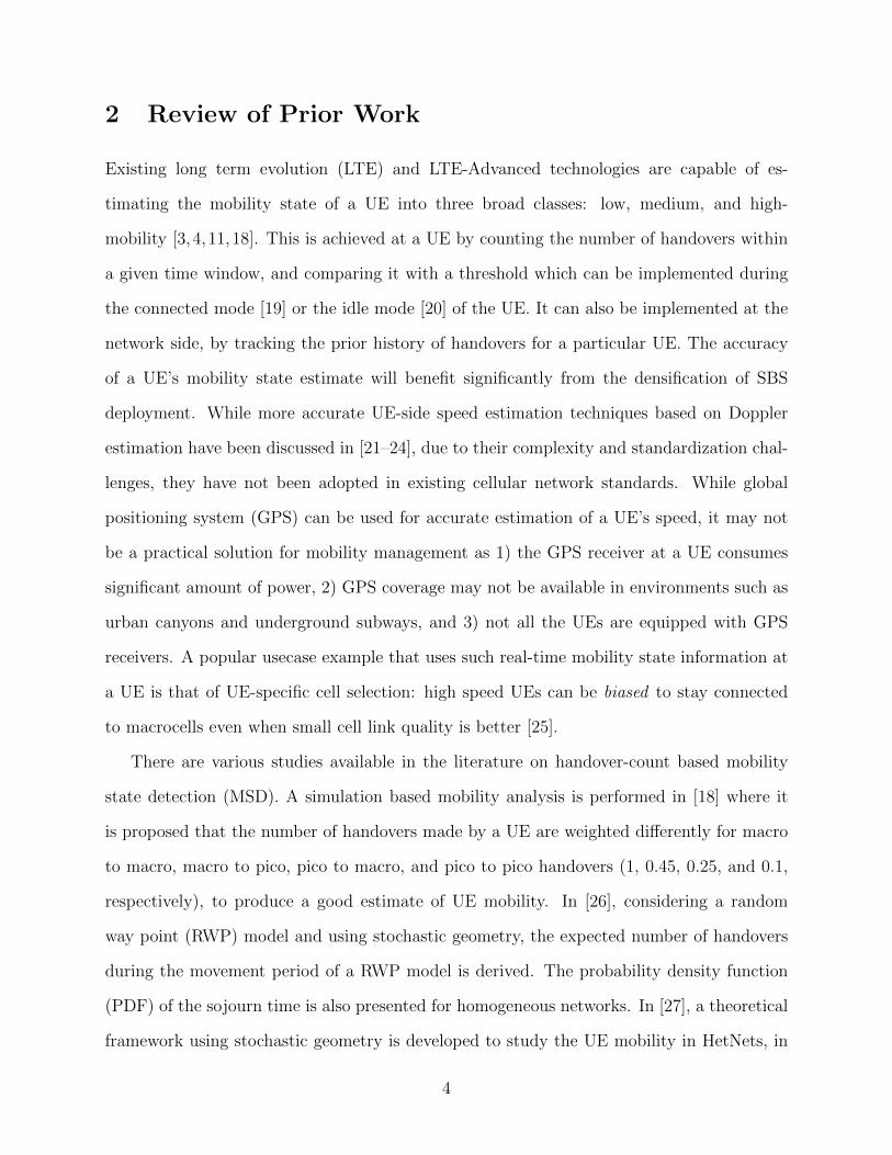
2 Review of Prior Work

Existing long term evolution (LTE) and LTE-Advanced technologies are capable of es-

timating the mobility state of a UE into three broad classes: low, medium, and high-

mobility [3,4,11,18]. This is achieved at a UE by counting the number of handovers within

a given time window, and comparing it with a threshold which can be implemented during

the connected mode [19] or the idle mode [20] of the UE. It can also be implemented at the

network side, by tracking the prior history of handovers for a particular UE. The accuracy

of a UE’s mobility state estimate will benefit significantly from the densification of SBS

deployment. While more accurate UE-side speed estimation techniques based on Doppler

estimation have been discussed in [21–24], due to their complexity and standardization chal-

lenges, they have not been adopted in existing cellular network standards. While global

positioning system (GPS) can be used for accurate estimation of a UE’s speed, it may not

be a practical solution for mobility management as 1) the GPS receiver at a UE consumes

significant amount of power, 2) GPS coverage may not be available in environments such as

urban canyons and underground subways, and 3) not all the UEs are equipped with GPS

receivers. A popular usecase example that uses such real-time mobility state information at

a UE is that of UE-specific cell selection: high speed UEs can be biased to stay connected

to macrocells even when small cell link quality is better [25].

There are various studies available in the literature on handover-count based mobility

state detection (MSD). A simulation based mobility analysis is performed in [18] where it

is proposed that the number of handovers made by a UE are weighted differently for macro

to macro, macro to pico, pico to macro, and pico to pico handovers (1, 0.45, 0.25, and 0.1,

respectively), to produce a good estimate of UE mobility. In [26], considering a random

way point (RWP) model and using stochastic geometry, the expected number of handovers

during the movement period of a RWP model is derived. The probability density function

(PDF) of the sojourn time is also presented for homogeneous networks. In [27], a theoretical

framework using stochastic geometry is developed to study the UE mobility in HetNets, in

4

which the expressions for vertical and horizontal handoff rates are derived. In [28], closed

form expressions of cross-tier handover rate and sojourn time in a small cell are provided

using stochastic geometry for a two-tier network. In another study [29], stochastic geometry

is used to derive the handover rate, which in turn is used to derive coverage probability of a

UE in HetNet by considering that the UE is mobile and a fraction of the handovers result

into failure.

A set of related works in the literature have studied the path prediction of UEs and the

handoff time estimation along the predicted path which can help in improving the quality

of service to the UEs. A destination and mobility path prediction model called DAMP is

proposed in [30], while a handoff time window estimation method and mobility-prediction-

aware bandwidth (MPBR) allocation scheme is presented in [31]. In [32], different methods

for predicting the future location of a UE based on prior knowledge of the UE’s mobility

are studied. A method for tracing UE’s location using semi-supervised graph Laplacian

approach is proposed in [33].

Despite the earlier work in [3,4,11,18–24,26,27,29–33], fundamental performance bounds

and optimum algorithms for handover-count based velocity estimation have not been studied

in the literature. The focus of this paper is on velocity estimation and MSD based on

the handover counts of a UE; path prediction and handoff time estimation techniques are

not considered. Mobility state estimation itself is an important topic in 3GPP Release-8

specifications, and being researched currently. Additionally, there are applications which

require velocity estimation at the UE side, in which case, implementing the path prediction

algorithms at a UE would be difficult. To our best knowledge, velocity estimation based on

handover counts at a UE has not been studied analytically in the literature, which is one of

the main contribution of this paper.

5

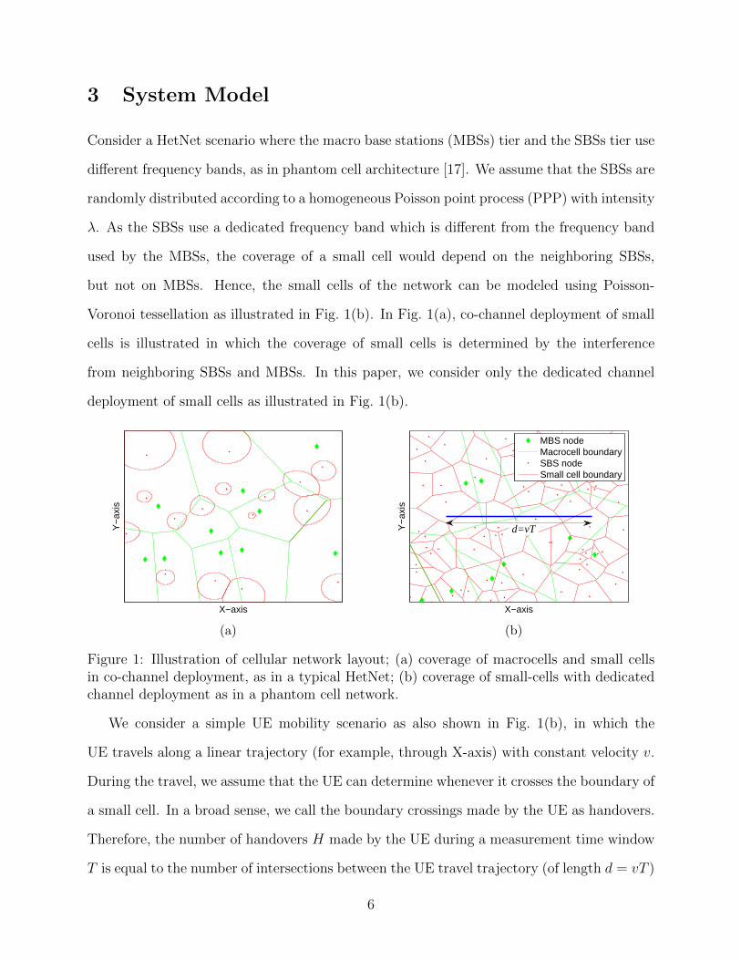
3 System Model

Consider a HetNet scenario where the macro base stations (MBSs) tier and the SBSs tier use

different frequency bands, as in phantom cell architecture [17]. We assume that the SBSs are

randomly distributed according to a homogeneous Poisson point process (PPP) with intensity

λ. As the SBSs use a dedicated frequency band which is different from the frequency band

used by the MBSs, the coverage of a small cell would depend on the neighboring SBSs,

but not on MBSs. Hence, the small cells of the network can be modeled using Poisson-

Voronoi tessellation as illustrated in Fig. 1(b). In Fig. 1(a), co-channel deployment of small

cells is illustrated in which the coverage of small cells is determined by the interference

from neighboring SBSs and MBSs. In this paper, we consider only the dedicated channel

deployment of small cells as illustrated in Fig. 1(b).

X−axis

Y−

axis

(a)

X−axis

Y−

axis

MBS nodeMacrocell boundarySBS nodeSmall cell boundary

d=vT

(b)

Figure 1: Illustration of cellular network layout; (a) coverage of macrocells and small cellsin co-channel deployment, as in a typical HetNet; (b) coverage of small-cells with dedicatedchannel deployment as in a phantom cell network.

We consider a simple UE mobility scenario as also shown in Fig. 1(b), in which the

UE travels along a linear trajectory (for example, through X-axis) with constant velocity v.

During the travel, we assume that the UE can determine whenever it crosses the boundary of

a small cell. In a broad sense, we call the boundary crossings made by the UE as handovers.

Therefore, the number of handovers H made by the UE during a measurement time window

T is equal to the number of intersections between the UE travel trajectory (of length d = vT )

6

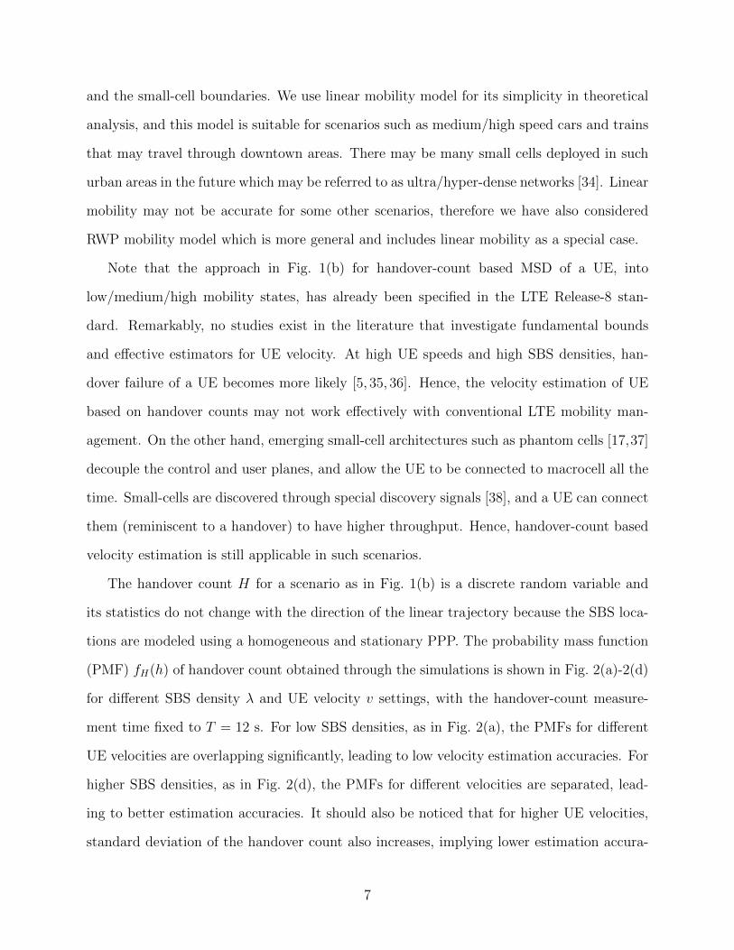
and the small-cell boundaries. We use linear mobility model for its simplicity in theoretical

analysis, and this model is suitable for scenarios such as medium/high speed cars and trains

that may travel through downtown areas. There may be many small cells deployed in such

urban areas in the future which may be referred to as ultra/hyper-dense networks [34]. Linear

mobility may not be accurate for some other scenarios, therefore we have also considered

RWP mobility model which is more general and includes linear mobility as a special case.

Note that the approach in Fig. 1(b) for handover-count based MSD of a UE, into

low/medium/high mobility states, has already been specified in the LTE Release-8 stan-

dard. Remarkably, no studies exist in the literature that investigate fundamental bounds

and effective estimators for UE velocity. At high UE speeds and high SBS densities, han-

dover failure of a UE becomes more likely [5, 35, 36]. Hence, the velocity estimation of UE

based on handover counts may not work effectively with conventional LTE mobility man-

agement. On the other hand, emerging small-cell architectures such as phantom cells [17,37]

decouple the control and user planes, and allow the UE to be connected to macrocell all the

time. Small-cells are discovered through special discovery signals [38], and a UE can connect

them (reminiscent to a handover) to have higher throughput. Hence, handover-count based

velocity estimation is still applicable in such scenarios.

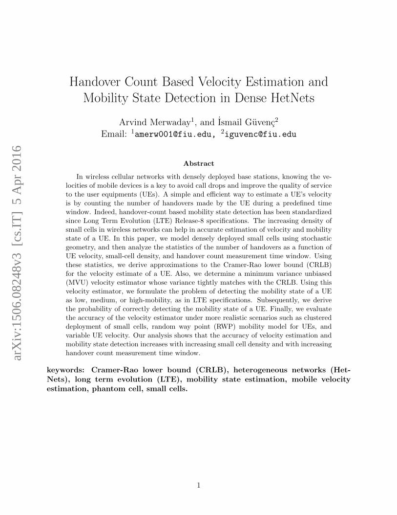
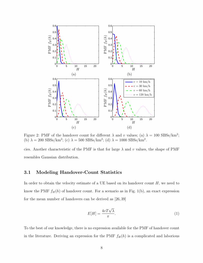
The handover count H for a scenario as in Fig. 1(b) is a discrete random variable and

its statistics do not change with the direction of the linear trajectory because the SBS loca-

tions are modeled using a homogeneous and stationary PPP. The probability mass function

(PMF) fH(h) of handover count obtained through the simulations is shown in Fig. 2(a)-2(d)

for different SBS density λ and UE velocity v settings, with the handover-count measure-

ment time fixed to T = 12 s. For low SBS densities, as in Fig. 2(a), the PMFs for different

UE velocities are overlapping significantly, leading to low velocity estimation accuracies. For

higher SBS densities, as in Fig. 2(d), the PMFs for different velocities are separated, lead-

ing to better estimation accuracies. It should also be noticed that for higher UE velocities,

standard deviation of the handover count also increases, implying lower estimation accura-

7

0 5 10 15 200

0.1

0.2

0.3

0.4

0.5

0.6

PMF

fH(h

)

H

(a)

0 5 10 15 200

0.1

0.2

0.3

0.4

0.5

0.6

PMF

fH(h

)

H

(b)

0 5 10 15 200

0.1

0.2

0.3

0.4

0.5

0.6

PMF

fH(h

)

H

(c)

0 5 10 15 200

0.1

0.2

0.3

0.4

0.5

0.6

PMF

fH(h

)

H

v = 10 km/h

v = 30 km/h

v = 60 km/h

v = 120 km/h

(d)

Figure 2: PMF of the handover count for different λ and v values; (a) λ = 100 SBSs/km2;(b) λ = 200 SBSs/km2; (c) λ = 500 SBSs/km2; (d) λ = 1000 SBSs/km2.

cies. Another characteristic of the PMF is that for large λ and v values, the shape of PMF

resembles Gaussian distribution.

3.1 Modeling Handover-Count Statistics

In order to obtain the velocity estimate of a UE based on its handover count H, we need to

know the PMF fH(h) of handover count. For a scenario as in Fig. 1(b), an exact expression

for the mean number of handovers can be derived as [26,39]

E[H] =4vT√λ

π. (1)

To the best of our knowledge, there is no expression available for the PMF of handover count

in the literature. Deriving an expression for the PMF fH(h) is a complicated and laborious

8

task, which might result into a mathematically intractable expression [39]. Hence, we derive

an approximation to the PMF fH(h) in this paper.

There are several papers in the literature where the PPP based parameters are approx-

imated rather than deriving the exact expressions due to the complexity involved in the

derivation of exact expressions. For example, in [40], geometrical characteristics of the

perimeter, area and number of edges in a 2-dimensional Voronoi cell, and volume, surface

area and number of faces in a 3-dimensional Voronoi cell are approximated by fitting gen-

eralized gamma distribution to the respective histograms. Similarly, the distributions of

2-dimensional cell area and 3-dimensional cell volume are approximated in [41] by fitting

some simple expressions.

In this paper, we derive two approximations to the PMF fH(h) for the handover count:

1) approximation f gH(h) derived using gamma distribution;

2) approximation fnH(h) derived using Gaussian distribution.

These two approximations to the handover count PMF will be discussed in more detail in

Section 4, and their accuracies will be further investigated and compared in Section 7.1.

4 Approximation of the Handover Count PMF Using

Gamma and Gaussian Distributions

In this section, two approximations for the PMF of handover count will be introduced.

In each approximation method, the parameters of a distribution (gamma distribution or

Gaussian distribution) will be approximated using the curve fitting tools in Matlab.

9

4.1 Approximation of the PMF of Handover Count using Gamma

Distribution

Gamma distribution has been commonly used in approximating the statistical distribution

of the parameters related to PPPs such as area, volume, number of edges, etc., of Poisson

Voronoi cells [40, 41]. It can be effectively used to approximate the handover count PMF.

The gamma PDF can be expressed using the shape parameter α > 0 and rate parameter

β > 0 as

f g(x) =βα

Γ(α)xα−1e−βx, for x ∈ (0,∞), (2)

where Γ(α) =∫∞

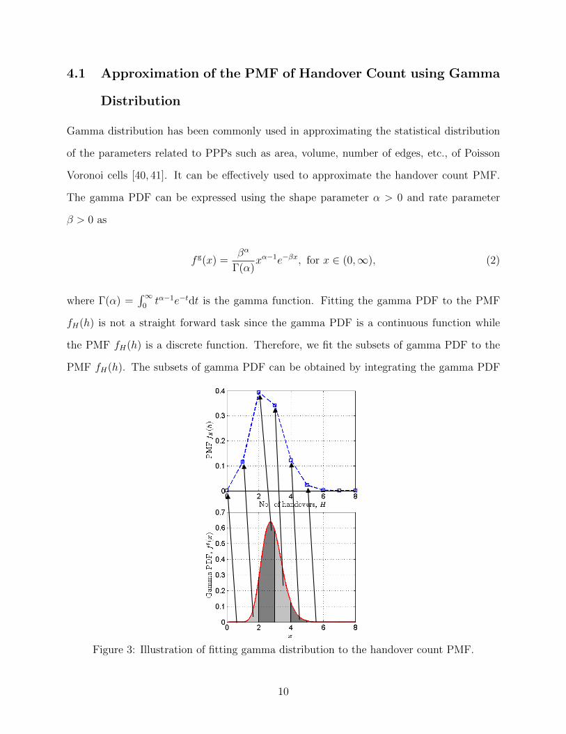
0tα−1e−tdt is the gamma function. Fitting the gamma PDF to the PMF

fH(h) is not a straight forward task since the gamma PDF is a continuous function while

the PMF fH(h) is a discrete function. Therefore, we fit the subsets of gamma PDF to the

PMF fH(h). The subsets of gamma PDF can be obtained by integrating the gamma PDF

Figure 3: Illustration of fitting gamma distribution to the handover count PMF.

10

between the integer values of x as illustrated in Fig. 3. Integrating the gamma PDF between

0 and 1 provides the PMF value for h = 0, integrating the gamma PDF between 1 and 2

provides the PMF value for h = 1, and so on. This process can be mathematically described

as:

f gH(h) =

∫ h+1

h

f g(x)dx, for h ∈ {0, 1, 2, ...}, (3)

where, f gH(h) is an approximation to the PMF fH(h). Substituting (2) into (3), we get

f gH(h) =

∫ h+1

h

βα

Γ(α)xα−1e−βxdx =

βα

Γ(α)

∫ h+1

h

xα−1e−βxdx, for h ∈ {0, 1, 2, ...}. (4)

With the change of variable x = t/β, we can rewrite (4) in its equivalent form as

f gH(h) =

βα

Γ(α)

∫ β(h+1)

βh

(t

β

)α−1

e−tdt

β=

1

Γ(α)

∫ β(h+1)

βh

tα−1e−tdt =Γ(α, βh, β(h+ 1)

)Γ(α)

, (5)

where, Γ(α, βh, β(h+ 1)

)=∫ β(h+1)

βhtα−1e−tdt is the generalized incomplete gamma function.

However, for the approximation in (5) to be accurate, the values for α and β parameters

should be chosen such that the mean squared error (MSE) between fH(h) and f gH(h) is

minimized.

Lemma 1. The α and β parameters for the approximation in (5) which minimize the MSE

between fH(h) and f gH(h) can be expressed as

α = 2.7 + 4d√λ, (6)

β = π +0.8

0.38 + d√λ, (7)

where d = vT is the distance traveled by UE during the handover-count measurement time.

Proof. See Appendix A.

11

Using (5)-(7), we can capture the statistical distribution of handover count if the SBS

density and the distance traveled by UE are known. Through (6) and (7), it can also be

noticed that the handover-count distribution depends on the distance traveled by UE, rather

than the UE velocity or the time period independently.

4.2 Approximation of the PMF of Handover Count using Gaus-

sian Distribution

In the previous section, approximation to the handover count PMF fH(h) was derived using

gamma distribution which resulted into an expression in integral form. In this section, we

will approximate the PMF fH(h) using Gaussian distribution which results into a closed

form expression for the handover-count PMF.

The PDF of Gaussian distribution can be expressed as a function of mean µ and variance

σ2:

fn (x) =1√

2πσ2e−

(x−µ)2

2σ2 . (8)

Since the PMF fH(h) is discrete and the Gaussian distribution in (8) is continuous, we

consider only non-negative integer samples of the Gaussian distribution for the fitting process.

Henceforth, the approximation to fH(h) can be expressed as,

fnH(h) =

1√2πσ2

e−(h−µ)2

2σ2 , for h ∈ {0, 1, 2, ...}. (9)

The values of µ and σ2 should be chosen to minimize the MSE between fH(h) and fnH(h).

Lemma 2. The µ and σ2 parameters for the approximation in (9) which minimize the MSE

12

between fH(h) and fnH(h) can be expressed as

µ =4d√λ

π, (10)

σ2 = 0.07 + 0.41d√λ, (11)

where d = vT is the distance traveled by the UE during the handover count measurement

time.

Proof. See Appendix B.

5 Cramer-Rao Lower Bound for Velocity Estimation

CRLB can be used to serve as a lower bound on the variance of an unbiased estimator [42].

An estimator is said to be unbiased if its expected value is same as the true value of the

parameter being estimated. An unbiased estimator whose variance can achieve the CRLB is

said to be an efficient estimator, and it can achieve minimum MSE among all the unbiased

estimators. In some scenarios, it might not be feasible to determine an efficient estimator. In

that case, the unbiased estimator with the smallest variance is said to be a MVU estimator.

In this section, we will derive the CRLB for velocity estimation using the mathematical

tools from estimation theory. Since we have two different approximations for the PMF of

the number of handovers, we will obtain two separate CRLB expressions.

5.1 CRLB Derivation using Gamma PMF Approximation

In this sub-section we will obtain the CRLB by considering the handover count PMF ap-

proximation that was derived using gamma distribution in Section 4.1.

Theorem 1. In a Poisson-Voronoi tessellation of small cells with SBS node density λ, let a

UE travel with velocity v over a linear trajectory and make H handovers over a time duration

13

T . If the PMF of the handover count can be expressed using f gH(H; v) as in (5), then the

CRLB for velocity estimation is given by

var(v) ≥ 1

E[(

∂ log fgH(H;v)

∂v

)2] , (12)

where, E[·] is the expectation operator with respect to H, and

∂ log f gH(h; v)

∂v=

4T√λβα

α2 Γ(α, βh, β(h+ 1))

[hα2F2(α, α;α + 1, α + 1;−βh)

− (h+ 1)α2F2(α, α;α + 1, α + 1;−β(h+ 1))]

− 4T√λ

Γ(α, βh, β(h+ 1))

[γ(α, βh) log(βh)− γ(α, β(h+ 1)) log(β(h+ 1))

]+

0.8T√λβα−1e−βh

[hα − e−β(h+ 1)α

]Γ(α, βh, β(h+ 1))(0.38 + vT

√λ)2

− 4T√λ ψ(α), (13)

where, ψ(·) is digamma function, γ(α, x) =∫ x

0tα−1e−tdt is lower incomplete gamma function,

and 2F2(a1, a2; b1, b2; z) is generalized hypergeometric function which is expressed as

2F2(a1, a2; b1, b2; z) =∞∑k=0

(a1)k(a2)k(b1)k(b2)k

zk

k!, (14)

where, (a)0 = 1 and (a)k = a(a+ 1)(a+ 2)...(a+ k − 1), for k ≥ 1.

Proof. See Appendix C.

Due to the complexity of expression in (13), it is impractical to derive the right hand

side (RHS) of (12) in closed form. For this reason, we can only find asymptotic CRLB by

numerically evaluating the RHS of (12). Through simulations, we generate N samples of the

random variable H and denote them as {Hn}, for n ∈ 1, 2, ..., N . Using these N samples,

14

we can numerically evaluate the asymptotic CRLB using

var(v) ≥ N∑Hmax

m=Hmin

(Nm

(∂ log fgH(m;v)

∂v

)2) , (15)

where, Hmax = max{Hn : ∀n ∈ 1, 2, ..., N}, is the maximum value of Hn, Hmin = min{Hn :

∀n ∈ 1, 2, ..., N}, is the minimum value of Hn, and Nm =∑N

n=1 1{Hn = m} is the number

of elements in the set {Hn} that are equal to m. Here, 1{·} is the indicator function whose

value is 1 if the condition inside the braces is true, 0 otherwise.

5.2 CRLB Derivation using Gaussian PMF Approximation

In this sub-section, we will obtain the CRLB by considering the PMF approximation using

Gaussian distribution that was derived in Section 4.2.

Theorem 2. In a Poisson-Voronoi tessellation of small cells with SBS node density λ, let a

UE travel with velocity v over a linear trajectory and make H handovers over a time duration

T . If the PMF of the handover count can be expressed using fnH(H; v) as in (9), then the

CRLB for velocity estimation is given by

var(v) ≥ 1(µvσ

)2+ 1

2

(0.41T

√λ

σ2

)2 . (16)

Proof. Consider the PMF approximation fnH(h) in (9) which can be represented as a general

Gaussian distribution, H ∼ N (µ, σ2) , where µ and σ2 are given by (10) and (11) respectively.

The Fisher information for the general Gaussian observations is given by [42, Section 3.9]

I(v) =

(∂µ

∂v

)21

σ2+

1

2 (σ2)2

(∂σ2

∂v

)2

=

(4T√λ

π

)21

σ2+

1

2 (σ2)2

(0.41T

√λ)2

. (17)

Using inverse of the Fisher information, the CRLB can be expressed as in (16).

15

5.3 Minimum Variance Unbiased Estimator for UE Velocity

In Section 4.1 and Section 4.2, two CRLB expressions were derived by considering gamma

and Gaussian distributions, respectively, for approximating the handover count PMF. In the

case of using gamma distribution, the CRLB expression was complicated and not in closed

form. On the other hand, in the case of using Gaussian distribution, the CRLB expression

was relatively simple and in closed form. Hence, in this sub-section, we will consider the

case with Gaussian distribution and derive an estimator v for a UE’s velocity, which takes

the number of handovers H as the input. We will further derive the mean and the variance

of this estimator and show that it is a MVU estimator.

To derive the MVU velocity estimator, we first use Neyman-Fisher factorization to find

the sufficient statistic for v [42, Section 5.4]. Then, we make use of Rao-Blackwell-Lehmann-

Scheffe (RBLS) theorem to find the MVUE [42, Section 5.5]. The Neyman-Fisher factoriza-

tion theorem states that if we can factor the PMF fnH(h) as

fnH(h) = g

(F(h), v

)r(h), (18)

where g is a function depending on h only through F(h) and r is a function depending only

on h, then F(h) is a sufficient statistic for v. Using (9) and letting F(h) = h, we can factor

the PMF fnH(h) in the form of (18) as

fnH(h) =

1√2πσ2

e−(F(h)−µ)2

2σ2︸ ︷︷ ︸ · 1︸︷︷︸, (19)

g(F(h), v

)r(h)

Therefore, the sufficient statistic for v is F(h) = h. The sufficient statistic can be used

to find the MVU estimator by determining a function s so that v = s(F) is an unbiased

estimator of v. By inspecting the relationship between the mean number of handovers H

16

and the velocity v in (1), we can formulate an estimator for v as:

v =πH

4T√λ. (20)

In order to evaluate whether this estimator is unbiased, the expectation of the above esti-

mator can be derived as

E[v] = E

[πH

4T√λ

]=

π

4T√λE[H] =

π

4T√λµ. (21)

Plugging (10) into (21), we get

E[v] =π

4T√λ

4vT√λ

π= v. (22)

Therefore, the estimator v expressed in (20) is unbiased. Since this estimator is derived

through RBLS theorem, it is an MVU estimator. To determine whether it is an efficient

estimator, we derive the variance of the MVU estimator as follows:

var(v) =var

(πH

4T√λ

)=

(π

4T√λ

)2

var(H) =

(vσ

µ

)2

. (23)

Comparing (23) with (16), we can notice that the variance of MVU estimator is greater than

the CRLB, and hence, the derived estimator is not an efficient estimator. Nevertheless, in

Section 7.3, we show that the variance of the MVU estimator is very close to the CRLB.

6 Mobility State Detection

In this section, we will perform statistical analysis of MSD, in which a UE is categorized into

one of the three different mobility states: low mobility, medium mobility and high mobility,

as in 3GPP LTE Release-8 specifications [18, 43, 44]. We assume that the unbiased velocity

estimator derived in Section 5.3 is used to estimate the UE velocity, and we will derive

17

expressions for the probabilities that a UE is categorized into each of the three mobility

states.

Using the estimated UE velocity v from (20), the UE can be categorized into one of

the three mobility states: low (SL), medium (SM), and high (SH), based on the following

conditions:

S =

SL if v ≤ vl,

SM if vl < v ≤ vu,

SH if v > vu,

(24)

where, S ∈ {SL, SM, SH} is the detected mobility state of the UE. The thresholds vl and vu

are the lower and upper velocity thresholds, respectively, based on which a UE is classified

into one of the three mobility states.

6.1 Mobility State Probabilities

For a given velocity v, we define mobility state probability as the probability that the UE

is categorized into a particular state. We can define the following three mobility state

probabilities:

P (S = SL; v)→Probability that the mobility state is detected as SL, for a velocity v;

P (S = SM; v)→Probability that the mobility state is detected as SM, for a velocity v;

P (S = SH; v)→Probability that the mobility state is detected as SH, for a velocity v.

For a given velocity v, as the number of handovers H is a random variable, the velocity v

estimated using (20) is also a random variable. Hence, there will be false alarms and missed

detections for calculating the mobility state.

Next, we derive analytic expressions for the mobility state probabilities. Using (20), we

18

can express the PMF of v as,

fv(ν) = P (v = ν) = P

(πH

4T√λ

= ν

)= P

(H =

4T√λν

π

)= fH

(4T√λν

π

)= fH(h), (25)

where, h = 4T√λν

π. Using the approximation of PMF fH(h) with Gaussian distribution as in

(9), we can approximate the PMF of v as,

fv(ν) =fH(h)

≈fnH(h) =

1√2πσ2

e−(h−µ)2

2σ2 , for h ∈ {0, 1, 2, ...}. (26)

Now, we can express the three mobility state probabilities as

P (S = SL; v) = P (v ≤ vl) ≈hl∑h=0

fnH(h), (27)

P (S = SM; v) = P (vl < v ≤ vu) ≈hu∑

h=hl+1

fnH(h), (28)

P (S = SH; v) = P (v > vu) ≈∞∑

h=hu+1

fnH(h), (29)

where, hl =⌊4T√λvl

π

⌋, and hu =

⌊4T√λvu

π

⌋, (30)

are the optimum lower and upper handover count thresholds for MSD, respectively. Given

the velocity thresholds vl and vu, the choice of handover count thresholds has a direct im-

pact on the probability of correctly detecting the mobility state of a UE based on its ve-

locity [45]. In (30), we have theoretically derived the handover-count thresholds for MSD

which are optimum for the given velocity thresholds. In other related works in the liter-

ature, the handover-count thresholds for MSD have been determined through simulations.

In [5, 45, 46], the handover-count thresholds for MSD are found heuristically by considering

the cumulative distribution function (CDF) plots of handover counts, for few different UE

velocities. In [47], the handover counts are assumed to be distributed as Gaussian PDF, and

19

the optimum handover-count thresholds are obtained by using the handover-count PDFs

for few different UE velocities. However, in these prior works, the optimum handover-count

thresholds are determined for some particular values of BS density and measurement time

windows. Moreover, the statistical relationship between the UE velocity and the handover

count is not considered. In this paper, we have derived general expressions for the optimum

handover-count thresholds as a function of SBS density λ, handover-count measurement time

T , and velocity thresholds (vl and vu).

6.2 Probability of Detection and Probability of False Alarm

The probability of detection is the probability that the mobility state of a UE is detected

correctly. Mathematically, it can be expressed as

PD =

P (S = SL; v) if v ≤ vl,

P (S = SM; v) if vl < v ≤ vu,

P (S = SH; v) if v > vu.

(31)

The probability of false alarm is the probability that the mobility state is detected incorrectly,

which can be mathematically expressed as PFA = 1− PD.

Consider an illustrative example in which the UE velocity is v = 60 km/h, SBS density

is λ = 1000 SBSs/km2, and handover-count measurement time is T = 12 s. The PMFs

fH(h) and fv(ν) are shown in Figs. 4(a) and 4(b), respectively, which were obtained through

Monte Carlo Simulations. In Fig. 4(b), the range of v is divided into three regions SL, SM

and SH that are separated from each other through the velocity thresholds vl = 40 km/h

and vu = 80 km/h. It can be noticed in Fig. 4(b) that even though the actual UE velocity

is a constant v = 60 km/h which belongs to SM state, the estimated velocity is spread into

a range of velocities. Hence, there is a small probability that the mobility state could be

erroneously detected as SL or SH states, which is the probability of false alarm PFA. On

the other hand, majority of the times the mobility state would be correctly detected as SM,

20

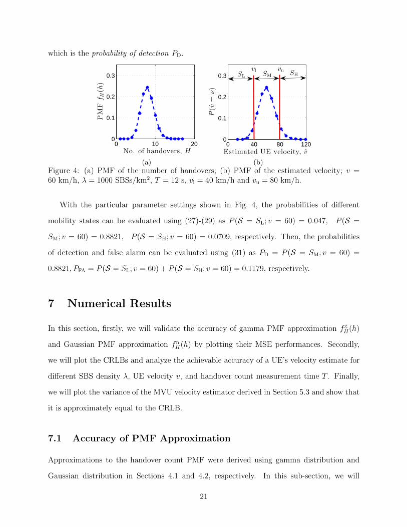
which is the probability of detection PD.

0 10 200

0.1

0.2

0.3

No. of handovers, H

PMF

fH(h

)

(a)

0 40 80 1200

0.1

0.2

0.3

Estimated UE velocity, v

P(v

=ν)

vlSL SM SH

vu

(b)Figure 4: (a) PMF of the number of handovers; (b) PMF of the estimated velocity; v =60 km/h, λ = 1000 SBSs/km2, T = 12 s, vl = 40 km/h and vu = 80 km/h.

With the particular parameter settings shown in Fig. 4, the probabilities of different

mobility states can be evaluated using (27)-(29) as P (S = SL; v = 60) = 0.047, P (S =

SM; v = 60) = 0.8821, P (S = SH; v = 60) = 0.0709, respectively. Then, the probabilities

of detection and false alarm can be evaluated using (31) as PD = P (S = SM; v = 60) =

0.8821, PFA = P (S = SL; v = 60) + P (S = SH; v = 60) = 0.1179, respectively.

7 Numerical Results

In this section, firstly, we will validate the accuracy of gamma PMF approximation f gH(h)

and Gaussian PMF approximation fnH(h) by plotting their MSE performances. Secondly,

we will plot the CRLBs and analyze the achievable accuracy of a UE’s velocity estimate for

different SBS density λ, UE velocity v, and handover count measurement time T . Finally,

we will plot the variance of the MVU velocity estimator derived in Section 5.3 and show that

it is approximately equal to the CRLB.

7.1 Accuracy of PMF Approximation

Approximations to the handover count PMF were derived using gamma distribution and

Gaussian distribution in Sections 4.1 and 4.2, respectively. In this sub-section, we will

21

0 1000 2000 3000 4000 5000

10−7

10−6

10−5

10−4

λ (SBSs/km2)

MS

E

v = 10 km/h

v = 30 km/h

v = 60 km/hv = 120 km/h

(a)

0 1000 2000 3000 4000 5000

10−6

10−5

10−4

10−3

λ (SBSs/km2)

MS

E

v = 60 km/h

v = 10 km/h

v = 30 km/h

v = 120 km/h

(b)

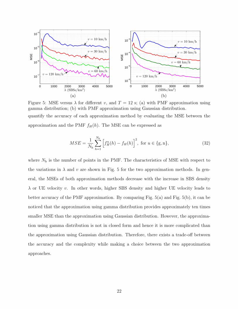
Figure 5: MSE versus λ for different v, and T = 12 s; (a) with PMF approximation usinggamma distribution; (b) with PMF approximation using Gaussian distribution.

quantify the accuracy of each approximation method by evaluating the MSE between the

approximation and the PMF fH(h). The MSE can be expressed as

MSE =1

Nh

Nh∑h=1

[fuH(h)− fH(h)

]2

, for u ∈ {g, n}, (32)

where Nh is the number of points in the PMF. The characteristics of MSE with respect to

the variations in λ and v are shown in Fig. 5 for the two approximation methods. In gen-

eral, the MSEs of both approximation methods decrease with the increase in SBS density

λ or UE velocity v. In other words, higher SBS density and higher UE velocity leads to

better accuracy of the PMF approximation. By comparing Fig. 5(a) and Fig. 5(b), it can be

noticed that the approximation using gamma distribution provides approximately ten times

smaller MSE than the approximation using Gaussian distribution. However, the approxima-

tion using gamma distribution is not in closed form and hence it is more complicated than

the approximation using Gaussian distribution. Therefore, there exists a trade-off between

the accuracy and the complexity while making a choice between the two approximation

approaches.

22

0 20 40 60 80 100 1205

10

15

20

25

30

35

UE velocity, v (km/h)

√

CRLB

(km/h)

λ = 100 SBSs/km2

λ = 200 SBSs/km2

λ = 500 SBSs/km2

λ = 1000 SBSs/km2

(a)

0 20 40 60 80 100 1200

5

10

15

20

25

30

35

UE velocity, v (km/h)

√

CRLB

(km/h)

λ = 100 SBSs/km2

λ = 200 SBSs/km2

λ = 500 SBSs/km2

λ = 1000 SBSs/km2

(b)

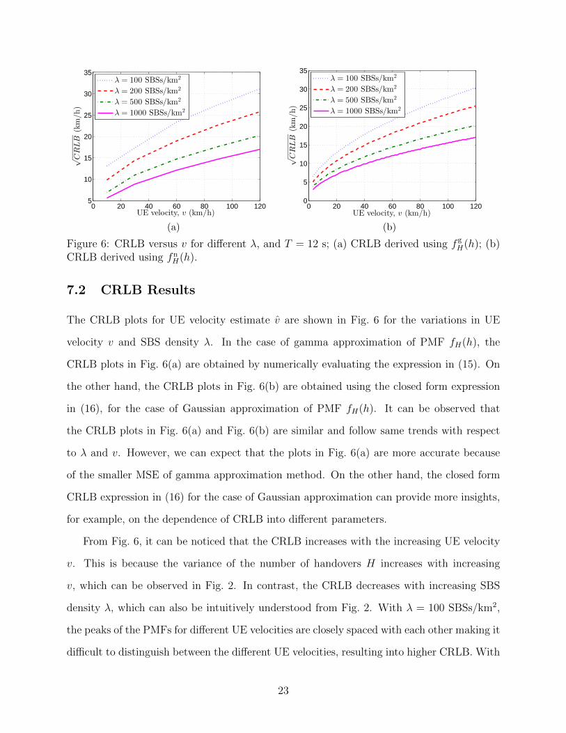
Figure 6: CRLB versus v for different λ, and T = 12 s; (a) CRLB derived using f gH(h); (b)

CRLB derived using fnH(h).

7.2 CRLB Results

The CRLB plots for UE velocity estimate v are shown in Fig. 6 for the variations in UE

velocity v and SBS density λ. In the case of gamma approximation of PMF fH(h), the

CRLB plots in Fig. 6(a) are obtained by numerically evaluating the expression in (15). On

the other hand, the CRLB plots in Fig. 6(b) are obtained using the closed form expression

in (16), for the case of Gaussian approximation of PMF fH(h). It can be observed that

the CRLB plots in Fig. 6(a) and Fig. 6(b) are similar and follow same trends with respect

to λ and v. However, we can expect that the plots in Fig. 6(a) are more accurate because

of the smaller MSE of gamma approximation method. On the other hand, the closed form

CRLB expression in (16) for the case of Gaussian approximation can provide more insights,

for example, on the dependence of CRLB into different parameters.

From Fig. 6, it can be noticed that the CRLB increases with the increasing UE velocity

v. This is because the variance of the number of handovers H increases with increasing

v, which can be observed in Fig. 2. In contrast, the CRLB decreases with increasing SBS

density λ, which can also be intuitively understood from Fig. 2. With λ = 100 SBSs/km2,

the peaks of the PMFs for different UE velocities are closely spaced with each other making it

difficult to distinguish between the different UE velocities, resulting into higher CRLB. With

23

10 20 30 40 50 605

10

15

20

25

Handover count measurement time, T (s)

√

CRLB

(km/h)

λ = 100 SBSs/km2

λ = 200 SBSs/km2

λ = 500 SBSs/km2

λ = 1000 SBSs/km2

(a)

10 20 30 40 50 605

10

15

20

25

Handover count measurement time, T (s)

√

CRLB

(km/h)

λ = 100 SBSs/km2

λ = 200 SBSs/km2

λ = 500 SBSs/km2

λ = 1000 SBSs/km2

(b)

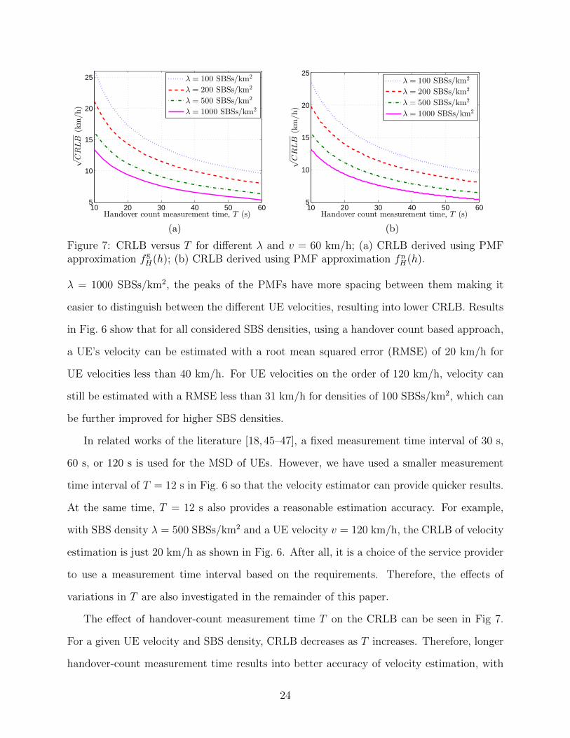
Figure 7: CRLB versus T for different λ and v = 60 km/h; (a) CRLB derived using PMFapproximation f g

H(h); (b) CRLB derived using PMF approximation fnH(h).

λ = 1000 SBSs/km2, the peaks of the PMFs have more spacing between them making it

easier to distinguish between the different UE velocities, resulting into lower CRLB. Results

in Fig. 6 show that for all considered SBS densities, using a handover count based approach,

a UE’s velocity can be estimated with a root mean squared error (RMSE) of 20 km/h for

UE velocities less than 40 km/h. For UE velocities on the order of 120 km/h, velocity can

still be estimated with a RMSE less than 31 km/h for densities of 100 SBSs/km2, which can

be further improved for higher SBS densities.

In related works of the literature [18, 45–47], a fixed measurement time interval of 30 s,

60 s, or 120 s is used for the MSD of UEs. However, we have used a smaller measurement

time interval of T = 12 s in Fig. 6 so that the velocity estimator can provide quicker results.

At the same time, T = 12 s also provides a reasonable estimation accuracy. For example,

with SBS density λ = 500 SBSs/km2 and a UE velocity v = 120 km/h, the CRLB of velocity

estimation is just 20 km/h as shown in Fig. 6. After all, it is a choice of the service provider

to use a measurement time interval based on the requirements. Therefore, the effects of

variations in T are also investigated in the remainder of this paper.

The effect of handover-count measurement time T on the CRLB can be seen in Fig 7.

For a given UE velocity and SBS density, CRLB decreases as T increases. Therefore, longer

handover-count measurement time results into better accuracy of velocity estimation, with

24

the assumption that the UE will continue traveling on a linear trajectory.

7.3 Variance of the MVU Velocity Estimator

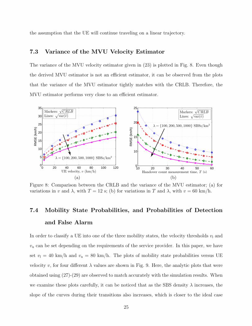
The variance of the MVU velocity estimator given in (23) is plotted in Fig. 8. Even though

the derived MVU estimator is not an efficient estimator, it can be observed from the plots

that the variance of the MVU estimator tightly matches with the CRLB. Therefore, the

MVU estimator performs very close to an efficient estimator.

0 20 40 60 80 100 1200

5

10

15

20

25

30

35

UE velocity, v (km/h)

RM

SE

(km

/h)

Markers:√CRLB

Lines:√

var(v)

λ = {100, 200, 500, 1000} SBSs/km2

(a)

10 20 30 40 50 605

10

15

20

25

Handover count measurement time, T (s)

RM

SE

(km

/h)

Markers:√CRLB

Lines:√

var(v)

λ = {100, 200, 500, 1000} SBSs/km2

(b)

Figure 8: Comparison between the CRLB and the variance of the MVU estimator; (a) forvariations in v and λ, with T = 12 s; (b) for variations in T and λ, with v = 60 km/h.

7.4 Mobility State Probabilities, and Probabilities of Detection

and False Alarm

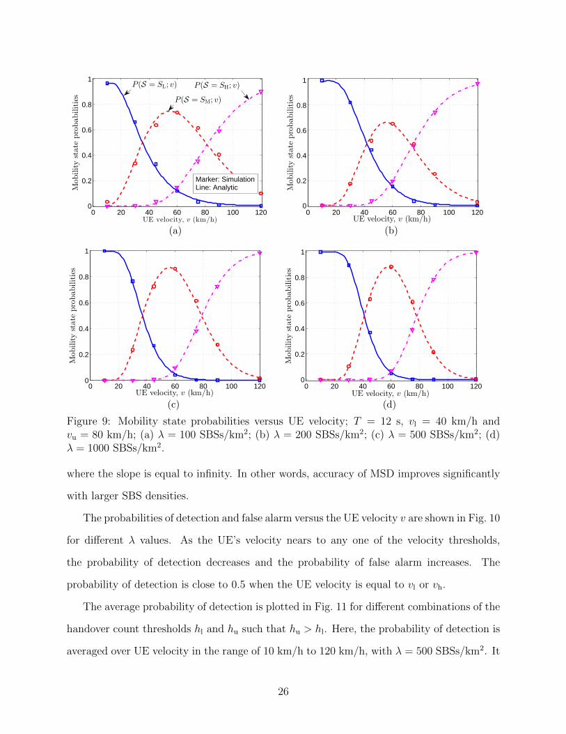
In order to classify a UE into one of the three mobility states, the velocity thresholds vl and

vu can be set depending on the requirements of the service provider. In this paper, we have

set vl = 40 km/h and vu = 80 km/h. The plots of mobility state probabilities versus UE

velocity v, for four different λ values are shown in Fig. 9. Here, the analytic plots that were

obtained using (27)-(29) are observed to match accurately with the simulation results. When

we examine these plots carefully, it can be noticed that as the SBS density λ increases, the

slope of the curves during their transitions also increases, which is closer to the ideal case

25

0 20 40 60 80 100 1200

0.2

0.4

0.6

0.8

1

UE velocity, v (km/h)

Mobilitystate

probabilities

Marker: SimulationLine: Analytic

P(S = SL; v)

P(S = SM; v)

P(S = SH; v)

(a)

0 20 40 60 80 100 1200

0.2

0.4

0.6

0.8

1

UE velocity, v (km/h)

Mobilitystate

probabilities

(b)

0 20 40 60 80 100 1200

0.2

0.4

0.6

0.8

1

UE velocity, v (km/h)

Mobilitystate

probabilities

(c)

0 20 40 60 80 100 1200

0.2

0.4

0.6

0.8

1

UE velocity, v (km/h)

Mobilitystate

probabilities

(d)

Figure 9: Mobility state probabilities versus UE velocity; T = 12 s, vl = 40 km/h andvu = 80 km/h; (a) λ = 100 SBSs/km2; (b) λ = 200 SBSs/km2; (c) λ = 500 SBSs/km2; (d)λ = 1000 SBSs/km2.

where the slope is equal to infinity. In other words, accuracy of MSD improves significantly

with larger SBS densities.

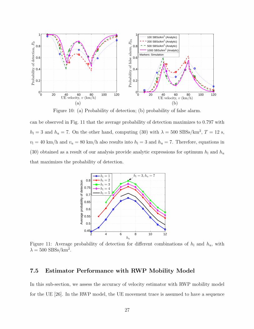
The probabilities of detection and false alarm versus the UE velocity v are shown in Fig. 10

for different λ values. As the UE’s velocity nears to any one of the velocity thresholds,

the probability of detection decreases and the probability of false alarm increases. The

probability of detection is close to 0.5 when the UE velocity is equal to vl or vh.

The average probability of detection is plotted in Fig. 11 for different combinations of the

handover count thresholds hl and hu such that hu > hl. Here, the probability of detection is

averaged over UE velocity in the range of 10 km/h to 120 km/h, with λ = 500 SBSs/km2. It

26

0 20 40 60 80 100 1200

0.2

0.4

0.6

0.8

1

UE velocity, v (km/h)

Probabilityofdetection,PD

(a)

0 20 40 60 80 100 1200

0.2

0.4

0.6

0.8

1

UE velocity, v (km/h)

Probabilityoffalsealarm

,PFA

100 SBSs/km2 (Analytic)

200 SBSs/km2 (Analytic)

500 SBSs/km2 (Analytic)

1000 SBSs/km2 (Analytic)

Markers: Simulation

(b)

Figure 10: (a) Probability of detection; (b) probability of false alarm.

can be observed in Fig. 11 that the average probability of detection maximizes to 0.797 with

hl = 3 and hu = 7. On the other hand, computing (30) with λ = 500 SBSs/km2, T = 12 s,

vl = 40 km/h and vu = 80 km/h also results into hl = 3 and hu = 7. Therefore, equations in

(30) obtained as a result of our analysis provide analytic expressions for optimum hl and hu

that maximizes the probability of detection.

2 4 6 8 10 120.45

0.5

0.55

0.6

0.65

0.7

0.75

0.8

hu

Ave

rage

pro

babi

lity

of d

etec

tion

hl = 1

hl = 2

hl = 3

hl = 4

hl = 5

hl = 3, hu = 7

Figure 11: Average probability of detection for different combinations of hl and hu, withλ = 500 SBSs/km2.

7.5 Estimator Performance with RWP Mobility Model

In this sub-section, we assess the accuracy of velocity estimator with RWP mobility model

for the UE [26]. In the RWP model, the UE movement trace is assumed to have a sequence

27

of quadruples which can be defined as {(Xn−1,Xn, Vn, Sn)}n∈N, where n denotes the n-th

movement period, Xn−1 and Xn denote the starting and target waypoints, respectively, dur-

ing the n-th movement period, Vn denotes the velocity, and Sn denotes the pause time at

the waypoint Xn. The angle between two consecutive waypoints is uniformly randomly dis-

tributed on [−π, π], while the transition length Ln = ‖Xn−Xn−1‖ between two consecutive

waypoints is i.i.d. and Rayleigh distributed with the CDF, P (L ≤ l) = 1−exp(−ξπl2), l ≥ 0,

where ξ is defined as the mobility parameter. Larger ξ statistically implies that the transition

lengths L are shorter and may be appropriate for mobile users walking. In contrast, smaller

ξ statistically implies longer transitions lengths which may be appropriate for driving users.

We performed simulations for a special case of the RWP mobility model in which the UE

velocity Vn ≡ v is a positive constant, and the pause times Sn = 0. The characteristics of

the RMSE of velocity estimator are shown in Fig. 12. It can be observed that the RMSE

increases with increasing v, and decreases with increasing T , similar to the characteristics

of the linear mobility model. The RMSE increases with the increasing mobility parameter

ξ. For large ξ, the UE switches its directions more number of times within the handover

count measurement time interval, leading to larger estimation errors. On the other hand,

for smaller ξ, the UE’s direction switch rate is smaller which results into smaller RMSE. As

ξ → 0, the RMSE of RWP mobility model converges to the RMSE of the linear mobility

model. This is because the direction switch rate tends to zero, and the UE follows a straight

line trajectory indefinitely.

7.6 Mobility State Detection with Variable UE Velocity

In this sub-section, we demonstrate the functionality of our MVU estimator with variable UE

velocity, and the effect of handover-count measurement time on estimation accuracy. Con-

sider an example in which a user is traveling in a train that is moving over a straight line tra-

jectory in a downtown region. Assume that the density of small cells is λ = 1000 SBSs/km2,

and handover counts are measured during regular intervals T . The actual velocity of UE

28

0 20 40 60 80 100 1200

5

10

15

20

25

30

35

40

UE velocity, v (km/h)

RMSE(km/h)

RWP mobility (ξ = 500 waypoints/km2)

RWP mobility (ξ = 200 waypoints/km2)

RWP mobility (ξ = 10 waypoints/km2)

Linear mobility (ξ → 0)

(a)

10 20 30 40 50 605

10

15

20

25

Handover count measurement time, T (s)

RMSE(km/h)

RWP mobility (ξ = 500 waypoints/km2)

RWP mobility (ξ = 200 waypoints/km2)

RWP mobility (ξ = 10 waypoints/km2)

Linear mobility (ξ → 0)

(b)

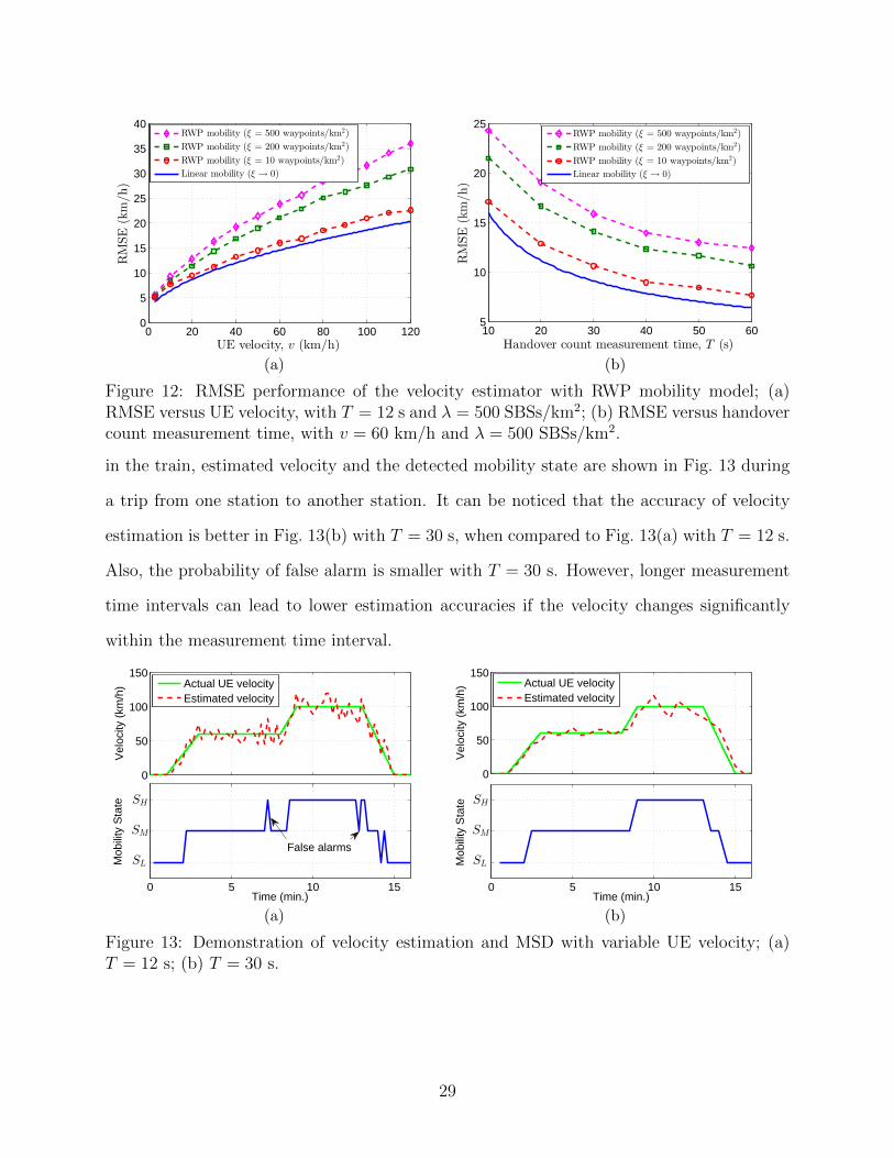
Figure 12: RMSE performance of the velocity estimator with RWP mobility model; (a)RMSE versus UE velocity, with T = 12 s and λ = 500 SBSs/km2; (b) RMSE versus handovercount measurement time, with v = 60 km/h and λ = 500 SBSs/km2.

in the train, estimated velocity and the detected mobility state are shown in Fig. 13 during

a trip from one station to another station. It can be noticed that the accuracy of velocity

estimation is better in Fig. 13(b) with T = 30 s, when compared to Fig. 13(a) with T = 12 s.

Also, the probability of false alarm is smaller with T = 30 s. However, longer measurement

time intervals can lead to lower estimation accuracies if the velocity changes significantly

within the measurement time interval.

0

50

100

150

Vel

ocity

(km

/h)

0 5 10 15Time (min.)

Mob

ility

Sta

te

Actual UE velocityEstimated velocity

False alarms

SH

SM

SL

(a)

0

50

100

150

Vel

ocity

(km

/h)

0 5 10 15Time (min.)

Mob

ility

Sta

te

Actual UE velocityEstimated velocity

SH

SM

SL

(b)

Figure 13: Demonstration of velocity estimation and MSD with variable UE velocity; (a)T = 12 s; (b) T = 30 s.

29

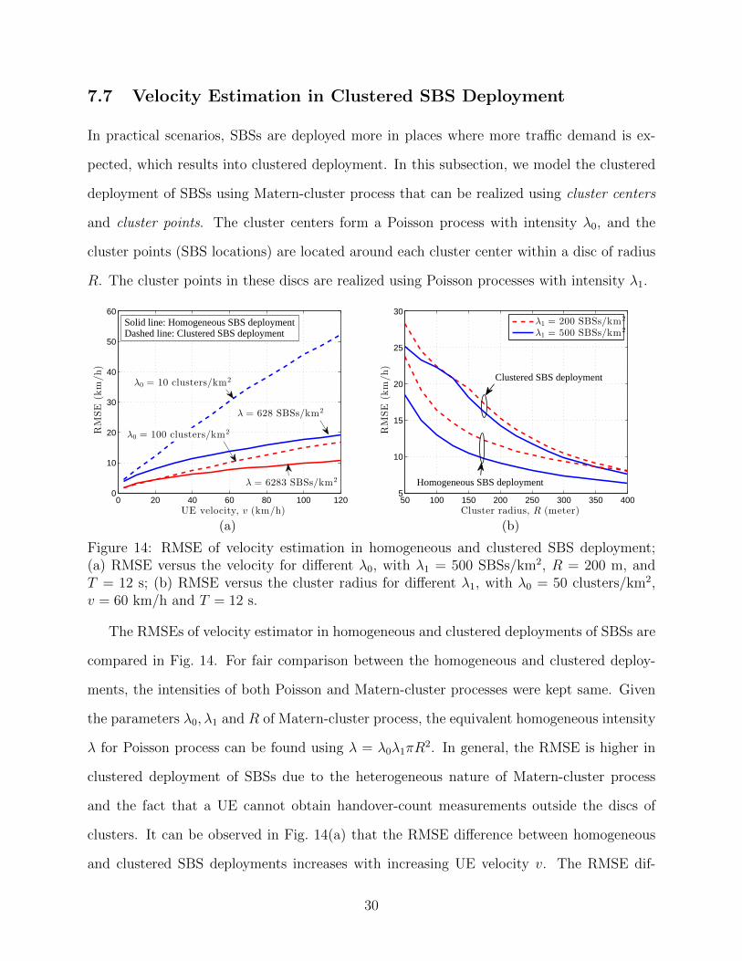
7.7 Velocity Estimation in Clustered SBS Deployment

In practical scenarios, SBSs are deployed more in places where more traffic demand is ex-

pected, which results into clustered deployment. In this subsection, we model the clustered

deployment of SBSs using Matern-cluster process that can be realized using cluster centers

and cluster points. The cluster centers form a Poisson process with intensity λ0, and the

cluster points (SBS locations) are located around each cluster center within a disc of radius

R. The cluster points in these discs are realized using Poisson processes with intensity λ1.

0 20 40 60 80 100 1200

10

20

30

40

50

60

UE velocity, v (km/h)

RMSE

(km/h)

λ0 = 10 clusters/km2

λ = 628 SBSs/km2

λ0 = 100 clusters/km2

λ = 6283 SBSs/km2

Solid line: Homogeneous SBS deploymentDashed line: Clustered SBS deployment

(a)

50 100 150 200 250 300 350 4005

10

15

20

25

30

Cluster radius, R (meter)

RMSE

(km/h)

λ1 = 200 SBSs/km2

λ1 = 500 SBSs/km2

Clustered SBS deployment

Homogeneous SBS deployment

(b)

Figure 14: RMSE of velocity estimation in homogeneous and clustered SBS deployment;(a) RMSE versus the velocity for different λ0, with λ1 = 500 SBSs/km2, R = 200 m, andT = 12 s; (b) RMSE versus the cluster radius for different λ1, with λ0 = 50 clusters/km2,v = 60 km/h and T = 12 s.

The RMSEs of velocity estimator in homogeneous and clustered deployments of SBSs are

compared in Fig. 14. For fair comparison between the homogeneous and clustered deploy-

ments, the intensities of both Poisson and Matern-cluster processes were kept same. Given

the parameters λ0, λ1 and R of Matern-cluster process, the equivalent homogeneous intensity

λ for Poisson process can be found using λ = λ0λ1πR2. In general, the RMSE is higher in

clustered deployment of SBSs due to the heterogeneous nature of Matern-cluster process

and the fact that a UE cannot obtain handover-count measurements outside the discs of

clusters. It can be observed in Fig. 14(a) that the RMSE difference between homogeneous

and clustered SBS deployments increases with increasing UE velocity v. The RMSE dif-

30

ference also increases significantly when λ0 decreases, for example, from 100 clusters/km2

to 10 clusters/km2. In Fig. 14(b), it can be seen that the RMSE difference decreases with

increasing R.

7.8 Velocity Estimation with Matern Hardcore Process for SBS

Locations

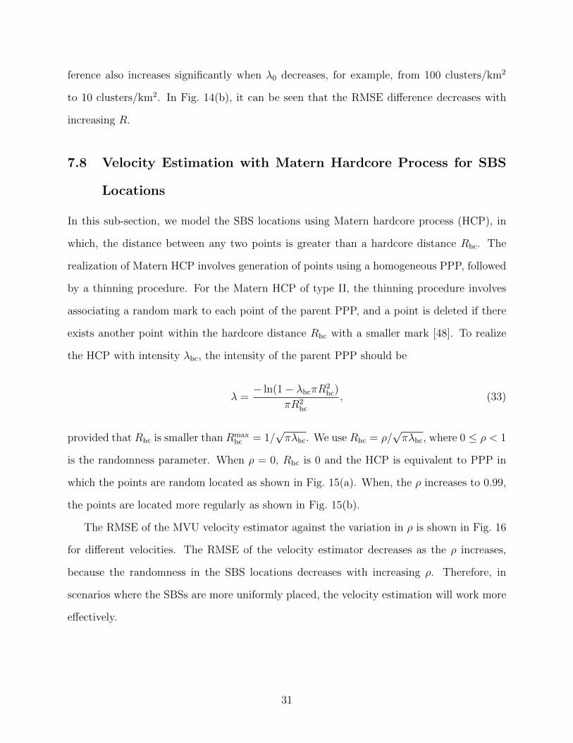
In this sub-section, we model the SBS locations using Matern hardcore process (HCP), in

which, the distance between any two points is greater than a hardcore distance Rhc. The

realization of Matern HCP involves generation of points using a homogeneous PPP, followed

by a thinning procedure. For the Matern HCP of type II, the thinning procedure involves

associating a random mark to each point of the parent PPP, and a point is deleted if there

exists another point within the hardcore distance Rhc with a smaller mark [48]. To realize

the HCP with intensity λhc, the intensity of the parent PPP should be

λ =− ln(1− λhcπR

2hc)

πR2hc

, (33)

provided that Rhc is smaller than Rmaxhc = 1/

√πλhc. We use Rhc = ρ/

√πλhc, where 0 ≤ ρ < 1

is the randomness parameter. When ρ = 0, Rhc is 0 and the HCP is equivalent to PPP in

which the points are random located as shown in Fig. 15(a). When, the ρ increases to 0.99,

the points are located more regularly as shown in Fig. 15(b).

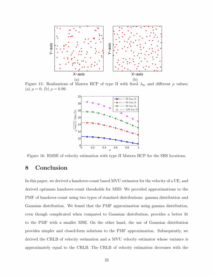
The RMSE of the MVU velocity estimator against the variation in ρ is shown in Fig. 16

for different velocities. The RMSE of the velocity estimator decreases as the ρ increases,

because the randomness in the SBS locations decreases with increasing ρ. Therefore, in

scenarios where the SBSs are more uniformly placed, the velocity estimation will work more

effectively.

31

X−axis

Y−

axis

(a)

X−axis

Y−

axis

(b)Figure 15: Realizations of Matern HCP of type II with fixed λhc and different ρ values;(a) ρ = 0; (b) ρ = 0.99.

0 0.2 0.4 0.6 0.8 18

10

12

14

16

18

20

22

ρ

√

var(v)(km/h)

v = 30 km/h

v = 60 km/h

v = 90 km/h

v = 120 km/h

Figure 16: RMSE of velocity estimation with type II Matern HCP for the SBS locations.

8 Conclusion

In this paper, we derived a handover-count based MVU estimator for the velocity of a UE, and

derived optimum handover-count thresholds for MSD. We provided approximations to the

PMF of handover-count using two types of standard distributions: gamma distribution and

Gaussian distribution. We found that the PMF approximation using gamma distribution,

even though complicated when compared to Gaussian distribution, provides a better fit

to the PMF with a smaller MSE. On the other hand, the use of Gaussian distribution

provides simpler and closed-form solutions to the PMF approximation. Subsequently, we

derived the CRLB of velocity estimation and a MVU velocity estimator whose variance is

approximately equal to the CRLB. The CRLB of velocity estimation decreases with the

32

increasing time interval for counting the number of handovers, which shows the trade-off

between the accuracy and the rapidness of velocity measurements.

The increasing density of small-cells in the future cellular networks is facilitates more

accurate UE velocity estimation, since the CRLB decreases with the increasing SBS den-

sity. Moreover, the probability of MSD also increases with the increasing SBS density. The

results with RWP mobility model showed that the accuracy of the velocity estimator de-

creases with the increasing randomness in UE’s mobility. On the other hand, results with

Matern-cluster process showed that the estimation accuracy is poorer with clustered SBS

deployment when compared to the homogeneous SBS deployment. Future research direc-

tions may include: path prediction of UEs, and development of algorithms to dynamically

adjust the measurement time interval depending on the past samples of estimated velocity.

Appendix A Approximating the α and β Parameters

of Gamma Distribution

In this appendix, we derive the expressions for α and β parameters through a heuristic

approach to minimize the MSE between the approximation f gH(h) and the PMF fH(h) of

the handover count. First, we briefly describe a property of PPP with respect to the scaling

of simulation space which will be used for the derivation of α and β parameters.

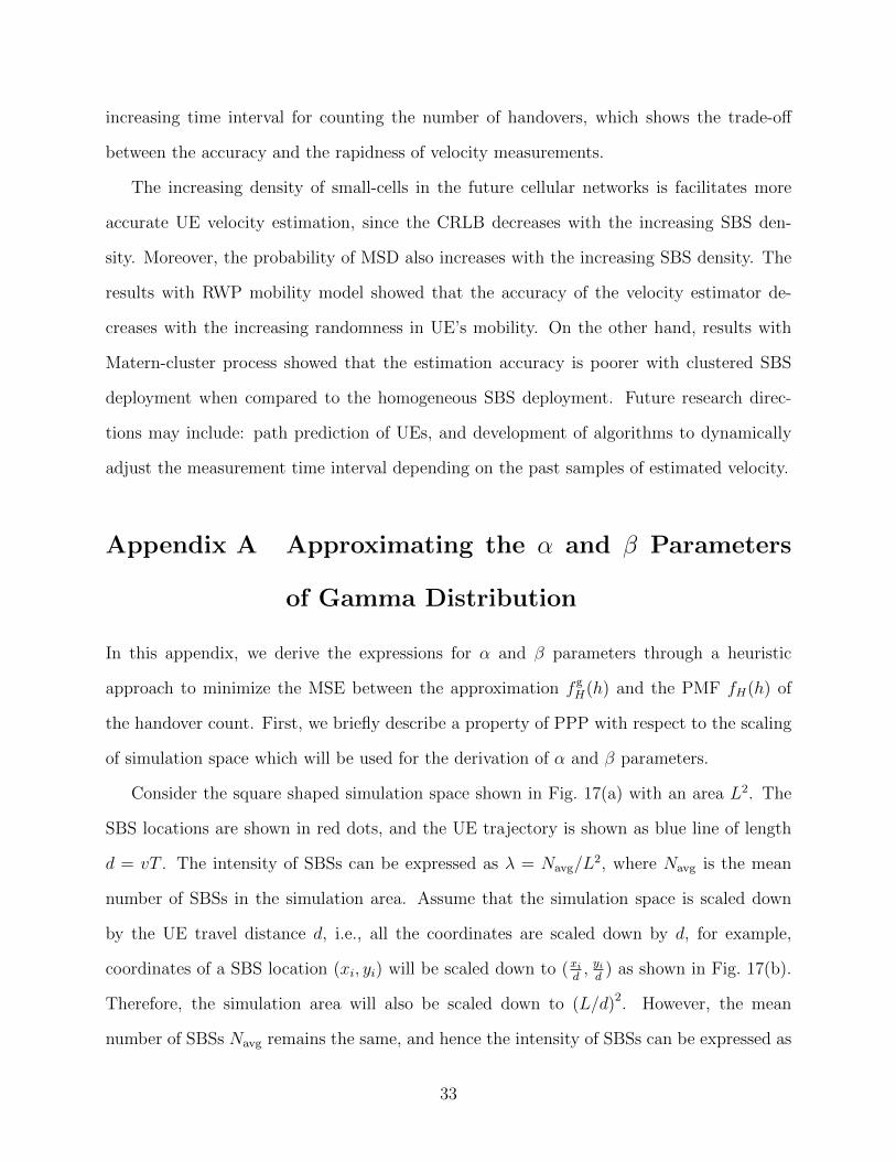
Consider the square shaped simulation space shown in Fig. 17(a) with an area L2. The

SBS locations are shown in red dots, and the UE trajectory is shown as blue line of length

d = vT . The intensity of SBSs can be expressed as λ = Navg/L2, where Navg is the mean

number of SBSs in the simulation area. Assume that the simulation space is scaled down

by the UE travel distance d, i.e., all the coordinates are scaled down by d, for example,

coordinates of a SBS location (xi, yi) will be scaled down to (xid, yid

) as shown in Fig. 17(b).

Therefore, the simulation area will also be scaled down to (L/d)2. However, the mean

number of SBSs Navg remains the same, and hence the intensity of SBSs can be expressed as

33

L

d = vT

( xi , y

i )

L

(a)

L/d

L/d

1

( xi/d , y

i/d )

(b)

Figure 17: Illustration for scaling down the simulation space.

λ′ = Navgd2/L2 = λd2. Here, the term λ′ is a function of λ and d, therefore, the statistics of

the handover count H can be expressed in terms of λ′ alone. For example, the mean number

of handovers in (1) can be expressed as E[H] = 4√λ′/π. Similarly, the parameters α and β

can also be approximated in terms of λ′.

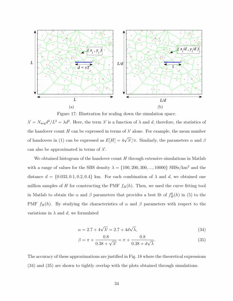
We obtained histogram of the handover count H through extensive simulations in Matlab

with a range of values for the SBS density λ = {100, 200, 300, ..., 10000} SBSs/km2 and the

distance d = {0.033, 0.1, 0.2, 0.4} km. For each combination of λ and d, we obtained one

million samples of H for constructing the PMF fH(h). Then, we used the curve fitting tool

in Matlab to obtain the α and β parameters that provides a best fit of f gH(h) in (5) to the

PMF fH(h). By studying the characteristics of α and β parameters with respect to the

variations in λ and d, we formulated

α = 2.7 + 4√λ′ = 2.7 + 4d

√λ, (34)

β = π +0.8

0.38 +√λ′

= π +0.8

0.38 + d√λ. (35)

The accuracy of these approximations are justified in Fig. 18 where the theoretical expressions

(34) and (35) are shown to tightly overlap with the plots obtained through simulations.

34

0 2000 4000 6000 8000 100000

50

100

150

200

λ (SBSs/km2)

αparameter

Lines: ApproximationMarkers: Simulation

d = {33, 100, 200, 400} m

0 2000 4000 6000 8000 100003

3.5

4

4.5

βparameter

λ (SBSs/km2)

d = {33, 100, 200, 400} m

Lines: ApproximationMarkers: Simulation

Figure 18: Approximations of the α and β parameters.

Appendix B Approximating the µ and σ2 Parameters

of Gaussian Distribution

In this appendix, we derive the expressions for µ and σ2 in (9) to minimize the MSE between

the approximation fnH(h) and the PMF fH(h) of the handover count. We equate µ to the

mean of handover count expressed in (1) as

µ =4vT√λ

π=

4d√λ

π. (36)

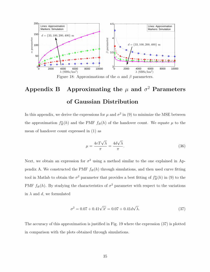
Next, we obtain an expression for σ2 using a method similar to the one explained in Ap-

pendix A. We constructed the PMF fH(h) through simulations, and then used curve fitting

tool in Matlab to obtain the σ2 parameter that provides a best fitting of fnH(h) in (9) to the

PMF fH(h). By studying the characteristics of σ2 parameter with respect to the variations

in λ and d, we formulated

σ2 = 0.07 + 0.41√λ′ = 0.07 + 0.41d

√λ. (37)

The accuracy of this approximation is justified in Fig. 19 where the expression (37) is plotted

in comparison with the plots obtained through simulations.

35

0 2000 4000 6000 8000 100000

5

10

15

20

λ (SBSs/km2)

σ2parameter

Lines: ApproximationMarkers: Simulation

d = {33, 100, 200, 400} m

Figure 19: Approximation of the σ2 parameter.

Appendix C Derivation of CRLB with Gamma Ap-

proximation for Handover Count PMF

In this appendix, CRLB for velocity estimation will be derived by considering the handover

count PMF in (5) that was derived using the gamma distribution. Taking the logarithm of

PMF will provide the log-likelihood function, which will then be differentiated with respect

to v. Finally, the derivative of log-likelihood function will be used to obtain the CRLB

expression. Consider the handover count PMF,

f gH(h; v) =

Γ(α, βh, β(h+ 1)

)Γ(α)

, (38)

where, the α and β parameters are given by (6) and (7), respectively. By taking the logarithm

of (38) and differentiating with respect to v, we get

∂

∂vlog f g

H(h; v) =∂

∂vlog Γ

(α, βh, β(h+ 1)

)− ∂

∂vlog Γ(α). (39)

Consider the first term in the RHS of (39). Let, z1 = βh and z2 = β(h + 1). Then, we

36

have

∂

∂vlog Γ

(α, βh, β(h+ 1)

)=

1

Γ(α, z1, z2)

∂

∂vΓ(α, z1, z2),

=1

Γ(α, z1, z2)

[∂

∂αΓ(α, z1, z2)

dα

dv+

∂

∂z1

Γ(α, z1, z2)dz1

dv+

∂

∂z2

Γ(α, z1, z2)dz2

dv

]. (40)

Each of the differentials in (40) can be derived to be

∂

∂αΓ(α, z1, z2) =

2F2(α, α;α + 1, α + 1;−z1)zα1α2

− 2F2(α, α;α + 1, α + 1;−z2)zα2α2

− γ(α, z1) log(z1) + γ(α, z2) log(z2),

∂

∂z1

Γ(α, z1, z2) = −e−z1zα−11 ,

∂

∂z2

Γ(α, z1, z2) = e−z2zα−12 ,

dα

dv= 4T

√λ,

dz1

dv=

−0.8hT√λ

(0.38 + vT√λ)2

,dz2

dv=−0.8(h+ 1)T

√λ

(0.38 + vT√λ)2

,

where, γ(α, x) =∫ x

0tα−1e−tdt is the lower incomplete gamma function, and 2F2(a1, a2; b1, b2; z)

is generalized hypergeometric function which can be expressed as

2F2(a1, a2; b1, b2; z) =∞∑k=0

(a1)k(a2)k(b1)k(b2)k

zk

k!, (41)

where, (a)0 = 1 and (a)k = a(a+ 1)(a+ 2)...(a+ k − 1), for k ≥ 1.

Now, consider the second term in RHS of (39), ∂∂v

log Γ(α) = ∂ log Γ(α)∂α

∂α∂v

. It is well

known that the logarithmic derivative of the gamma function is the digamma function ψ(·).

Therefore,

∂

∂vlog Γ(α) = ψ(α)

∂α

∂v= ψ(α)

∂

∂v(2.7 + 4vT

√λ) = 4T

√λ ψ(α). (42)

37

Using the equations (40)-(42), we can express (39) as:

∂

∂vlog f g

H(h; v) =4T√λβα

α2Γ(α, βh, β(h+ 1)

)[hα2F2(α, α;α + 1, α + 1;−βh)

− (h+ 1)α2F2

(α, α;α + 1, α + 1;−β(h+ 1)

)]− 4T

√λ

Γ(α, βh, β(h+ 1)

)[γ(α, βh) log(βh)− γ(α, β(h+ 1)

)log(β(h+ 1)

)]+

0.8T√λβα−1e−βh

[hα − e−β(h+ 1)α

]Γ(α, βh, β(h+ 1)

)(0.38 + vT

√λ)2

− 4T√λ ψ(α). (43)

By squaring (43) and evaluating the expectation over H, we obtain the Fisher information

as

I(v) = E

[(∂ log f g

H(H; v)

∂v

)2]. (44)

By taking the reciprocal of Fisher information, we can express the CRLB for v as in (12).

Acknowledgment

This research was supported in part by the U.S. National Science Foundation under the

Grant CNS-1406968.

References

[1] “Cisco Visual Networking Index: Global Mobile Data Traffic Forecast Update, 2013-2018 (White Paper),” Cisco Systems, Feb. 2014.

[2] Qualcomm, “The 1000x mobile data challenge: More small cells, more spectrum, higherefficiency,” Nov. 2013.

[3] D. L. Perez, I. Guvenc, and X. Chu, “Mobility management challenges in 3GPP het-erogeneous networks,” IEEE Commun. Mag., vol. 50, no. 12, pp. 70–78, Dec. 2012.

[4] ——, “Mobility enhancements for heterogeneous networks through interference coor-dination,” in Proc IEEE Wireless Commun. and Networking Conf. Workshops (WC-NCW), Paris, France, April 2012, pp. 69–74.

38

[5] 3GPP TR 36.839, “Evolved universal terrestrial radio access (E-UTRA); mobility en-hancements in heterogeneous networks,” Tech. Rep. V11.1.0, Jan. 2013.

[6] A. Merwaday, S. Mukherjee, and I. Guvenc, “On the capacity analysis of HetNets withrange expansion and eICIC,” in Proc. IEEE Global Commun. Conf. (GLOBECOM),Atlanta, GA, Dec. 2013, pp. 4257–4262.

[7] ——, “HetNet capacity with reduced power subframes,” in Proc. IEEE Wireless Com-mun. and Networking Conf. (WCNC), Istanbul, Turkey, Apr. 2014, pp. 1380–1385.

[8] ——, “Capacity analysis of LTE-Advanced HetNets with reduced power subframes andrange expansion,” EURASIP J. Wireless Commun. Networking, vol. 2014, no. 189, 2014.

[9] H. S. Dhillon, R. K. Ganti, F. Baccelli, and J. G. Andrews, “Modeling and analysisof K-tier downlink heterogeneous cellular networks,” IEEE J. Select. Areas Commun.,vol. 30, no. 3, pp. 550–560, Apr. 2012.

[10] Samsung, “Mobility support to pico cells in the co-channel HetNet deployment,” Stock-holm, Sweden, Mar. 2010, 3GPP Standard Contribution (R2-104017).

[11] J. Puttonen, N. Kolehmainen, T. Henttonen, and J. Kaikkonen, “On idle mode mobilitystate detection in evloved UTRAN,” in Proc. IEEE Int. Conf. Information Technology:New Generations, Las Vegas, NV, Apr. 2009, pp. 1195–1200.

[12] J. Niu, D. Lee, T. Su, G. Li, and X. Ren, “User classification and scheduling in LTEdownlink systems with heterogeneous user mobilities,” IEEE Trans. Wireless Commun.,vol. 12, no. 12, pp. 6205–6213, Dec. 2013.

[13] J. Niu, T. Su, G. Li, D. Lee, and Y. Fu, “Joint transmission mode selection and schedul-ing in LTE downlink MIMO systems,” IEEE Wireless Commun. Letters, vol. 3, no. 2,pp. 173–176, April 2014.

[14] S. M. Musa and N. F. Mir, “An analytical approach for mobility load balancing inwireless networks,” J. Computing and Inform. Technol., vol. 19, no. 3, pp. 169–176,2011.

[15] A. Dua, F. Lu, and V. Sethuraman, “Speed-adaptive channel quality indicator (cqi)estimation,” U.S. Patent 20120163207 A1, June 28, 2012.

[16] A. Prasad, P. Lunden, O. Tirkkonen, and C. Wijting, “Energy-efficient flexible inter-frequency scanning mechanism for enhanced small cell discovery,” in Proc. IEEE Veh.Technol. Conf. (VTC Spring), Dresden, Germany, June 2013, pp. 1–5.

[17] H. Ishii, Y. Kishiyama, and H. Takahashi, “A novel architecture for LTE-B :C-plane/U-plane split and phantom cell concept,” in Proc. IEEE Global Telecommun. Conf.(GLOBECOM) Workshops, 2012, pp. 624–630.

[18] S. Barbera, P. Michaelsen, M. Saily, and K. Pedersen, “Improved mobility performancein LTE co-channel hetnets through speed differentiated enhancements,” in Proc. IEEEGlobecom Workshops (GC Wkshps), 2012, pp. 426–430.

39

[19] 3GPP, “Evolved universal terrestrial radio access (E-UTRA); radio resource control(RRC); protocol specification, (TS 36.331).”

[20] 3GPP TS 36.304, “User Equipment (UE) procedures in idle mode,” 3GPP-TSG RAN,bb, Tech. Rep. 8.5.0, Mar. 2009.

[21] M. Ishii and M. Iwamura, “User device and method in mobile communicationsystem,” European Patent No: 2187671 A1, May 2010. [Online]. Available:https://www.google.com/patents/EP2187671A1

[22] A. Sampath and J. Holtzman, “Estimation of maximum Doppler frequency for handoffdecisions,” in Proc. IEEE Veh. Technol. Conf. (VTC), Secaucus, NJ, May 1993, pp.859–862.

[23] B. Zhou and S. Blostein, “Estimation of maximum Doppler frequency for handoff deci-sions,” in Proc. Sixth Can. Workshop on Info. Theory, June 1999, pp. 111–114.

[24] L. Zhou and S. D. Blostein, “Recursive maximum likelihood estimation of maximumDoppler frequency of a sampled fading signal,” in Proc. Biennial Sym. on Commun.,2000, pp. 361–365.

[25] J. Pang, Q. JIANG, G. Shen, and D. Wang, “Method, apparatus, and systemfor biasing adjustment of cell range expansion,” Oct. 2 2014, wO PatentApp. PCT/IB2014/000,572. [Online]. Available: http://www.google.com/patents/WO2014155197A1?cl=en

[26] X. Lin, R. Ganti, P. Fleming, and J. Andrews, “Towards understanding the fundamen-tals of mobility in cellular networks,” IEEE Trans. Wireless Commun., vol. 12, no. 4,pp. 1686–1698, April 2013.

[27] W. Bao and B. Liang, “Handoff rate analysis in heterogeneous cellular networks: Astochastic geometric approach,” in Proc. ACM Int. Conf. on Modeling, Analysis andSimulation of Wireless and Mobile Systems, Montreal, QC, Canada, Sept. 2014, pp.95–102.

[28] Y. Hong, X. Xu, M. Tao, J. Li, and T. Svensson, “Cross-tier handover analyses in smallcell networks: A stochastic geometry approach,” in Proc. IEEE Int. Conf. Commun.(ICC), London, UK, June 2015, pp. 3429–3434.

[29] S. Sadr and R. Adve, “Handoff rate and coverage analysis in multi-tier heterogeneousnetworks,” IEEE Trans. Wireless Commun., vol. 14, no. 5, pp. 2626–2638, Jan. 2015.

[30] A. Nadembega, A. Hafid, and T. Taleb, “A destination and mobility path predictionscheme for mobile networks,” IEEE Trans. Veh. Technol., vol. 64, no. 6, pp. 2577–2590,2015.

[31] ——, “Mobility-prediction-aware bandwidth reservation scheme for mobile networks,”IEEE Trans. Veh. Technol., vol. 64, no. 6, pp. 2561–2576, 2015.

40

[32] T. Anagnostopoulos, C. Anagnostopoulos, and S. Hadjiefthymiades, “Efficient locationprediction in mobile cellular networks,” Int. J. Wireless Inform. Networks, vol. 19, no. 2,pp. 97–111, 2012.

[33] J. Pan, S. Pan, J. Yin, L. Ni, and Q. Yang, “Tracking mobile users in wireless net-works via semi-supervised colocalization,” IEEE Trans. Pattern Analysis and MachineIntelligence, vol. 34, no. 3, pp. 587–600, 2012.

[34] Nokia Networks, “Evolution to ultra-dense networks.” [Online]. Available: http://networks.nokia.com/portfolio/latest-launches/evolution-to-ultra-dense-networks

[35] H.-S. Park, A.-S. Park, J.-Y. Lee, and B.-C. Kim, “Two-step handover for LTE het-net mobility enhancements,” in Proc. IEEE Int. Conf. ICT Convergence (ICTC), JejuIsland, Korea, Oct 2013, pp. 763–766.

[36] D. Lopez-Perez, I. Guvenc, and X. Chu, “Theoretical analysis of handover failure andping-pong rates for heterogeneous networks,” in Proc. IEEE Int. Conf. Commun. (ICC),Ottawa, ON, June 2012, pp. 6774–6779.

[37] NTT DOCOMO, “5G radio access: Requirements, concept and technologies,” WhitePaper, July 2014. [Online]. Available: https://www.nttdocomo.co.jp/english/binary/pdf/corporate/technology/\whitepaper 5g/DOCOMO 5G White Paper.pdf

[38] Huawei, HiSilicon, “Efficient discovery of small cells and the configurations,” Tech. Rep.3GPP TSG RAN R1-130895, Apr. 2013.

[39] J. Moller, Lectures On Random Voronoi Tessellations. Springer-Verlag, 1994.

[40] M. Tanemura, “Statistical distributions of poisson voronoi cells in two and three dimen-sions,” Forma, vol. 18, no. 4, pp. 221–247, 2003.

[41] J.-S. Ferenc and Z. Nda, “On the size distribution of poisson voronoi cells,” Physica A:Statistical Mechanics and its Applications, vol. 385, no. 2, pp. 518 – 526, 2007.

[42] S. M. Kay, Fundamentals of Statistical Signal Processing: Estimation Theory. Prentice-Hall, Inc., 1993.

[43] 3GPP, “Overview of 3GPP release 8,” Tech. Rep. V0.3.3, Sep. 2014.

[44] Huawei, HiSilicon, “Further evaluation on enhancements of mobility state estimation inhetnet,” Tech. Rep. 3GPP TSG RAN R2-121250, Mar. 2012.

[45] M. Mehta, N. Akhtar, and A. Karandikar, “Enhanced mobility state estimation in LTEhetnets,” in Proc. National Conf. Commun. (NCC), Mumbai, India, Feb 2015, pp. 1–6.

[46] H. Shen, K. Liu, D. Xiao, and Y. He, “The enhancements of UE mobility state estimationin the Het-Net of the LTE-A system,” in Proc. Int. Conf. Information Technol. andSoftware Engineering, ser. Lecture Notes in Electrical Engineering, W. Lu, G. Cai,W. Liu, and W. Xing, Eds. Springer Berlin Heidelberg, 2013, vol. 210, pp. 99–106.

41

[47] J. Turkka, T. Henttonen, and T. Ristaniemi, “Self-optimization of LTE mobility stateestimation thresholds,” in Proc. IEEE Wireless Commun. and Networking Conf. Work-shops (WCNCW), Istanbul, Turkey, April 2014, pp. 161–165.

[48] M. Haenggi, “Mean interference in hard-core wireless networks,” IEEE Commun. Lett.,vol. 15, no. 8, pp. 792–794, 2011.

42