Handout 2: structured programming • Logical expressions and operators • Decision making

– if

– else

– elseif

• Loop structures – for loops – while loops

• How to create your own functions (“function M-files”) • Global variables • Examples

– Optimization of irrigation channel design

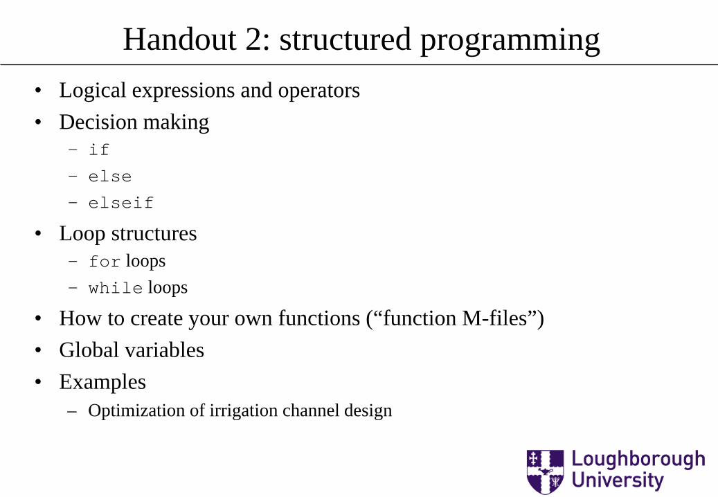
Decision making: use of conditional statements Conditional statements allow one to

introduce decision making into a computer program.

Logical expressions in MATLAB These take the form

variable1 relational_operator variable2

where variable1 and variable2 are MATLAB

scalar variables or constants, and relational_operator is one of:

Relational operator Interpretation < Less than <= Less than or equal to > Greater than >= Greater than or equal to == Equal to ~= Not equal to

Real life examples: 1. “If I get a pay rise I will buy a new car” 2. “If I get a pay rise of at least £100/month I

will buy a new car, else I will put the rise into savings”

3. “If I get a pay rise of at least £100/month, I will buy a new car, else if the rise is greater than £50 per month, I will buy a new stereo, else I will put the rise into savings.

Logical expressions The statement “I get a pay rise”, “I get a pay

rise of at least £100/month”, etc. are examples of logical expressions: they are either true (1) or false (0).

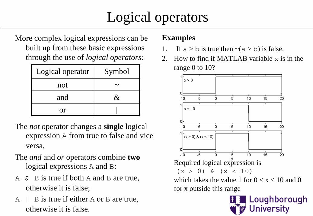
Logical operators More complex logical expressions can be

built up from these basic expressions through the use of logical operators:

The not operator changes a single logical

expression A from true to false and vice versa,

The and and or operators combine two logical expressions A and B:

A & B is true if both A and B are true, otherwise it is false;

A | B is true if either A or B are true, otherwise it is false.

Examples 2. How to find if MATLAB variable x is in the

range 0 to 10? Required logical expression is (x > 0) & (x < 10) which takes the value 1 for 0 < x < 10 and 0 for x outside this range

Logical operator Symbol

not ~ and & or |

1. If a > b is true then ~(a > b) is false.

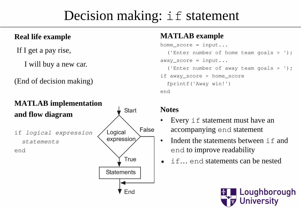
Decision making: if statement Real life example (End of decision making) MATLAB implementation and flow diagram

if logical expression

statements

end

MATLAB example home_score = input...

('Enter number of home team goals > ');

away_score = input...

('Enter number of away team goals > ');

if away_score > home_score

fprintf('Away win!')

end

Notes • Every if statement must have an

accompanying end statement • Indent the statements between if and

end to improve readability • if… end statements can be nested

If I get a pay rise,

I will buy a new car.

Decision making: else statement Real life example If I get a pay rise of at least £100 per month, I will buy a new car; (End of decision making) MATLAB implementation and flow diagram

if logical expression

statement group 1

else

statement group 2

end

MATLAB example if (away_score > home_score)

fprintf('Away team win!')

else

fprintf('Home team win or draw')

end else,

I will put the pay rise into savings.

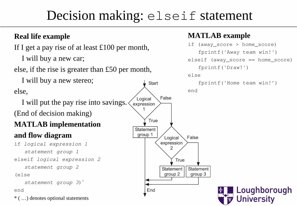
Decision making: elseif statement Real life example If I get a pay rise of at least £100 per month, I will buy a new car; else, if the rise is greater than £50 per month, I will buy a new stereo; else, I will put the pay rise into savings. (End of decision making) MATLAB implementation and flow diagram if logical expression 1

statement group 1

elseif logical expression 2

statement group 2

(else

statement group 3)*

end

* ( …) denotes optional statements

MATLAB example if (away_score > home_score)

fprintf('Away team win!')

elseif (away_score == home_score)

fprintf('Draw!')

else

fprintf('Home team win!’)

end

Loop structures in MATLAB

Each repetition of the loop is a pass. There are two types of loop in MATLAB: 1. The for loop where the number of

passes is known in advance 2. The while loop where the looping

terminates when a specified condition is satisfied (number of passes is not known in advance)

for loop: MATLAB implementation for loop variable = m:s:n

statements

end

for loop: meaning in words loop variable is a standard MATLAB

variable that starts with the value m.

statements are executed, and on reaching end, control is returned to for

Another pass through the loop occurs with loop variable incremented by s

The process is repeated until the loop variable reaches n

Notes on for loops • Every for statement must have an

accompanying end statement • Indent the statements between for and

end to improve readability • for… end loops can be nested

A loop is a structure for repeating a calculation a number of times.

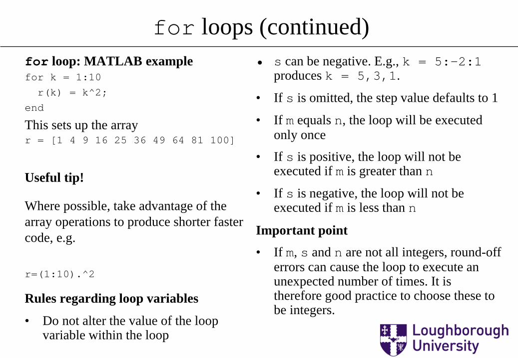
for loops (continued) for loop: MATLAB example for k = 1:10

r(k) = k^2;

end

This sets up the array r = [1 4 9 16 25 36 49 64 81 100]

Useful tip!

r=(1:10).^2

Rules regarding loop variables

• Do not alter the value of the loop variable within the loop

• s can be negative. E.g., k = 5:-2:1 produces k = 5,3,1.

• If s is omitted, the step value defaults to 1

• If m equals n, the loop will be executed only once

• If s is positive, the loop will not be executed if m is greater than n

• If s is negative, the loop will not be executed if m is less than n

Important point • If m, s and n are not all integers, round-off

errors can cause the loop to execute an unexpected number of times. It is therefore good practice to choose these to be integers.

Where possible, take advantage of the array operations to produce shorter faster code, e.g.

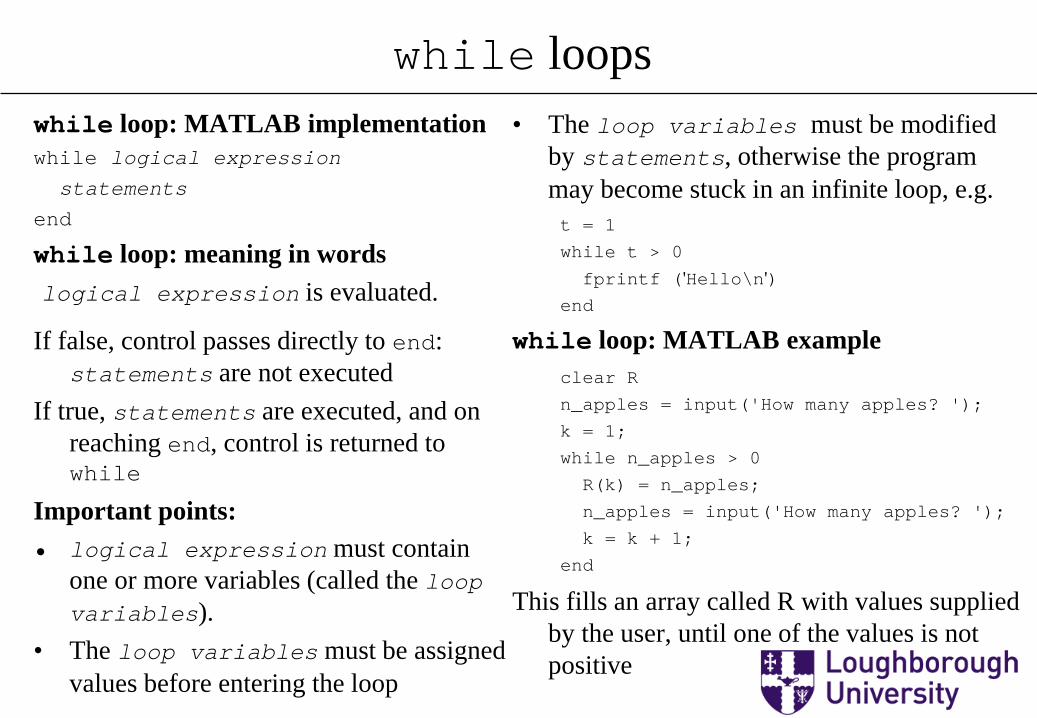
while loops while loop: MATLAB implementation while logical expression

statements

end

while loop: meaning in words

If false, control passes directly to end: statements are not executed

If true, statements are executed, and on reaching end, control is returned to while

Important points: • logical expression must contain

one or more variables (called the loop variables).

• The loop variables must be assigned values before entering the loop

• The loop variables must be modified by statements, otherwise the program may become stuck in an infinite loop, e.g. t = 1

while t > 0

fprintf ('Hello\n') end

while loop: MATLAB example clear R

n_apples = input('How many apples? ');

k = 1;

while n_apples > 0

R(k) = n_apples;

n_apples = input('How many apples? ');

k = k + 1;

end

This fills an array called R with values supplied by the user, until one of the values is not positive

logical expression is evaluated.

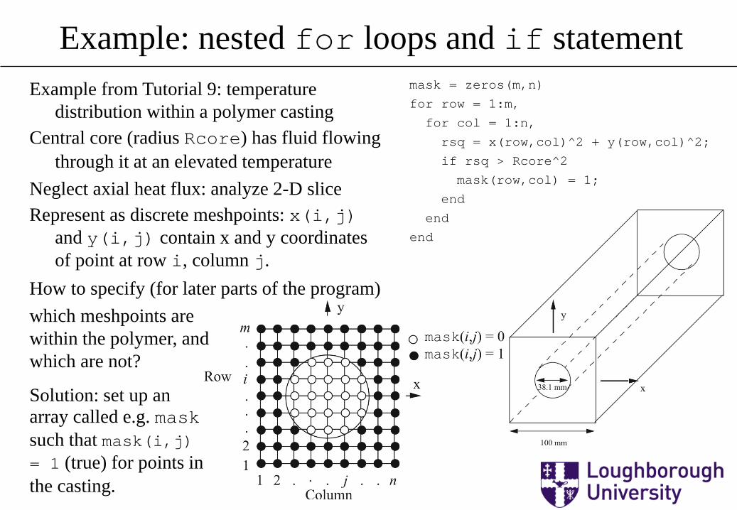
Example: nested for loops and if statement mask = zeros(m,n)

for row = 1:m,

for col = 1:n,

rsq = x(row,col)^2 + y(row,col)^2;

if rsq > Rcore^2

mask(row,col) = 1;

end

end

end

Example from Tutorial 9: temperature distribution within a polymer casting

Central core (radius Rcore) has fluid flowing through it at an elevated temperature

Neglect axial heat flux: analyze 2-D slice Represent as discrete meshpoints: x(i,j)

and y(i,j) contain x and y coordinates of point at row i, column j.

How to specify (for later parts of the program) which meshpoints are within the polymer, and which are not?

Solution: set up an array called e.g. mask such that mask(i,j) = 1 (true) for points in the casting.

Logical expressions involving arrays When logical expressions are evaluated,

they return a value of 0 or 1 which can be written to a MATLAB variable in the usual way.

A MATLAB statement such as y = x > 0

is therefore perfectly valid. It means “evaluate the logical expression ‘x > 0’, which will give the value 1 or 0, and store this in memory location y”

The general form is

var3 = var1 rel_op var2

where var1, var2 and var3 are

MATLAB variables, and rel_op is one of the 6 relational operators.

Powerful commands can be written in particularly compact form when either var1 or var2 (or both) are arrays. (NB if both are arrays, they must be of the same size).

The relational operator is then applied element by element, generating for each element a value 0 or 1. The result is written into a new array called var3.

Example

9 lines from previous slide replaced by 1! Make sure you understand how this

statement works.

mask = (x.^2 + y.^2) > Rcore^2;

Why do we need to create functions? 3 main reasons:

– Long programs are difficult to understand: structure into small blocks to aid readability

– Often need to perform same set of operations at more than one location – avoid duplication of unnecessary lines of code

– Can debug and test code separately Function M-files are M-files that can

accept input arguments and return output arguments, unlike script M-files which are just a collection of MATLAB instructions

[out1,out2,…,outn] =

function_name(in1,in2,…,inm) where in1,in2,…,inm are the m input

variables and out1,out2,…,outn are the n output variables. The sizes of the input and output arrays do not necessarily correspond to one another, but depend on the function.

The input and output variables are commonly called input and output arguments or parameters

The general expression for calling a function that returns more than one variable is:

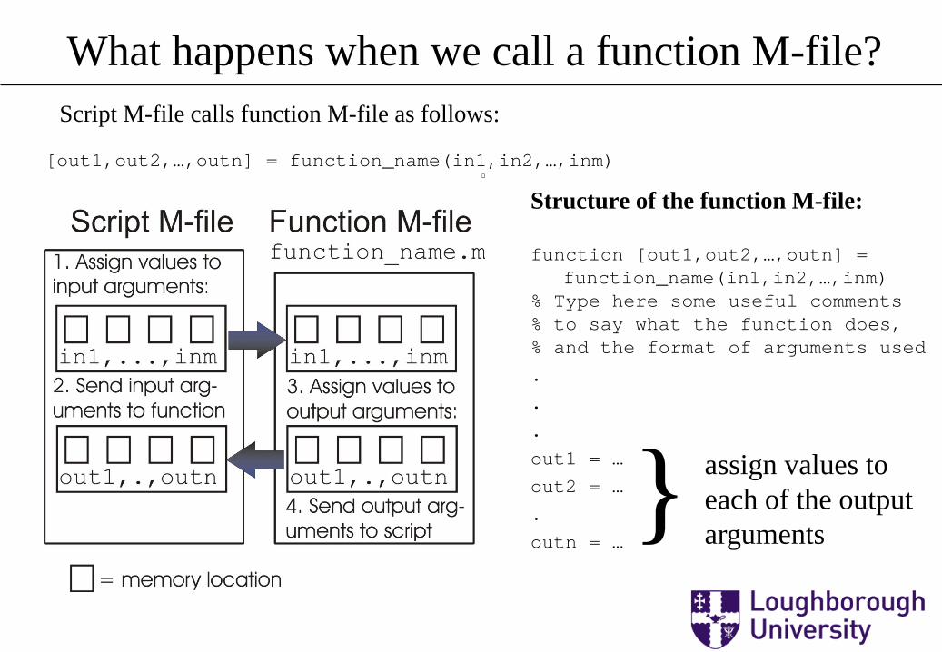
What happens when we call a function M-file?

Structure of the function M-file:

function [out1,out2,…,outn] = function_name(in1,in2,…,inm)

% Type here some useful comments % to say what the function does, % and the format of arguments used

.

.

.

out1 = …

out2 = …

.

outn = …

[out1,out2,…,outn] = function_name(in1,in2,…,inm)

} assign values to each of the output arguments

Script M-file calls function M-file as follows:

Important points for function M-files 1. The first line of the function M-file

must be a function definition line that specifies the input and output arguments

2. If there is only one output variable, the square brackets can be dispensed with: function out1 = function_name(in1,in2,…inm);

3. function_name should be chosen to help you remember what the function actually does, and must be the same as the name of the M-file

4. Provide useful comments on lines 2 onwards since these will be printed on the screen if you type help function_name

5. Variables are local to the function: variables with the same name can appear in both script M-file and function M-file; changes made in one will not affect the value in the other (use global statement to access the variables if necessary – see later)

6. Both input and output variables can be scalars or 1-D or 2-D arrays

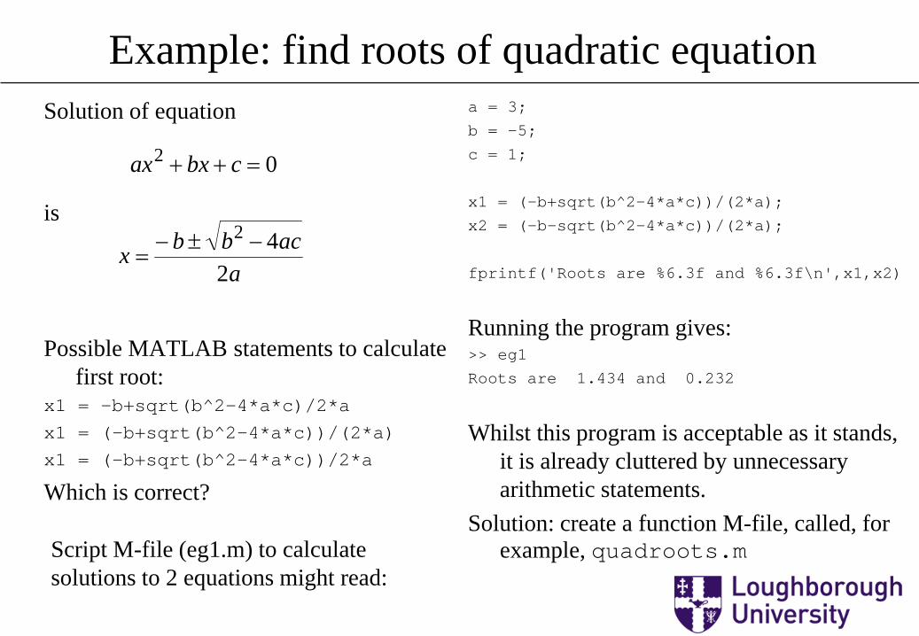
Example: find roots of quadratic equation Solution of equation is Possible MATLAB statements to calculate

first root: x1 = -b+sqrt(b^2-4*a*c)/2*a

x1 = (-b+sqrt(b^2-4*a*c))/(2*a)

x1 = (-b+sqrt(b^2-4*a*c))/2*a

Which is correct?

a = 3;

b = -5;

c = 1;

x1 = (-b+sqrt(b^2-4*a*c))/(2*a);

x2 = (-b-sqrt(b^2-4*a*c))/(2*a);

fprintf('Roots are %6.3f and %6.3f\n',x1,x2)

Running the program gives: >> eg1

Roots are 1.434 and 0.232

Whilst this program is acceptable as it stands, it is already cluttered by unnecessary arithmetic statements.

Solution: create a function M-file, called, for example, quadroots.m

02 =++ cbxax

aacbbx

242 −±−

=

Script M-file (eg1.m) to calculate solutions to 2 equations might read:

Example: script M-file calling function M-file

Script and function M-files in same folder

Function M-file comment lines provide useful help information

Script M-file called in usual way from command window

Script M-file calls function M-file

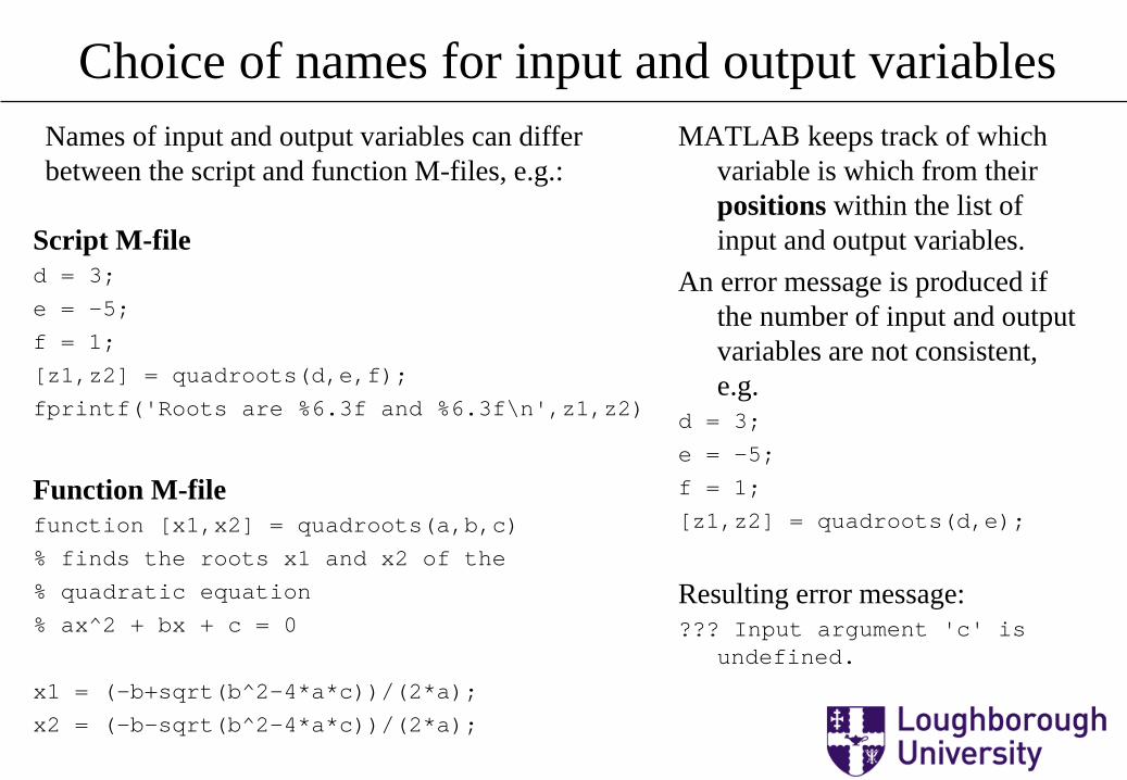
Choice of names for input and output variables

Script M-file d = 3;

e = -5;

f = 1;

[z1,z2] = quadroots(d,e,f);

fprintf('Roots are %6.3f and %6.3f\n',z1,z2)

Function M-file function [x1,x2] = quadroots(a,b,c)

% finds the roots x1 and x2 of the

% quadratic equation

% ax^2 + bx + c = 0

x1 = (-b+sqrt(b^2-4*a*c))/(2*a);

x2 = (-b-sqrt(b^2-4*a*c))/(2*a);

MATLAB keeps track of which variable is which from their positions within the list of input and output variables.

An error message is produced if the number of input and output variables are not consistent, e.g.

d = 3;

e = -5;

f = 1;

[z1,z2] = quadroots(d,e);

Resulting error message: ??? Input argument 'c' is

undefined.

Names of input and output variables can differ between the script and function M-files, e.g.:

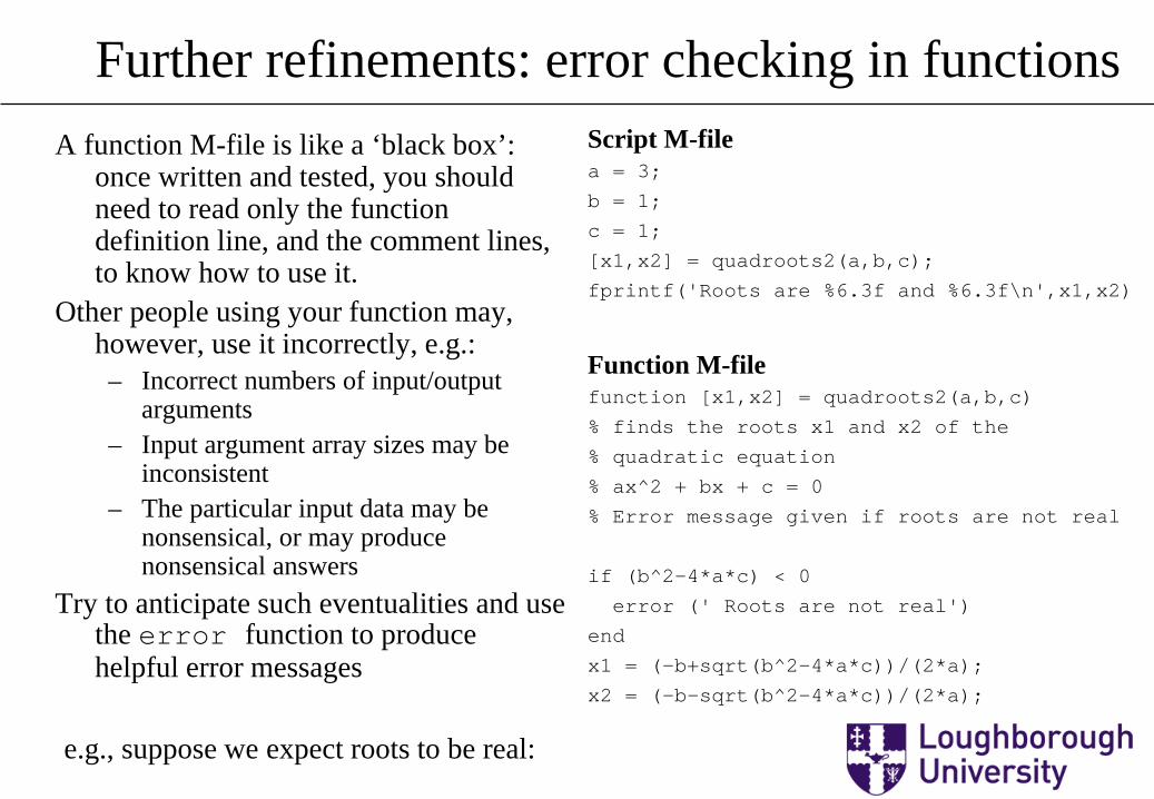
Further refinements: error checking in functions A function M-file is like a ‘black box’:

once written and tested, you should need to read only the function definition line, and the comment lines, to know how to use it.

Other people using your function may, however, use it incorrectly, e.g.:

– Incorrect numbers of input/output arguments

– Input argument array sizes may be inconsistent

– The particular input data may be nonsensical, or may produce nonsensical answers

Try to anticipate such eventualities and use the error function to produce helpful error messages

Script M-file a = 3;

b = 1;

c = 1;

[x1,x2] = quadroots2(a,b,c);

fprintf('Roots are %6.3f and %6.3f\n',x1,x2)

Function M-file function [x1,x2] = quadroots2(a,b,c)

% finds the roots x1 and x2 of the

% quadratic equation

% ax^2 + bx + c = 0

% Error message given if roots are not real

if (b^2-4*a*c) < 0

error (' Roots are not real')

end

x1 = (-b+sqrt(b^2-4*a*c))/(2*a);

x2 = (-b-sqrt(b^2-4*a*c))/(2*a);

e.g., suppose we expect roots to be real:

Use of global variables Variables are normally local to the script

or function M-file containing them. This situation can be modified by

declaring specified variables to be global in all the files requiring access to these variables, by using the global command (followed by a list of the variables) near the start of each M-file.

Important point: This provides an additional route for data

transfer as follows:

the list must be identical, and in the same order, in each M-file.

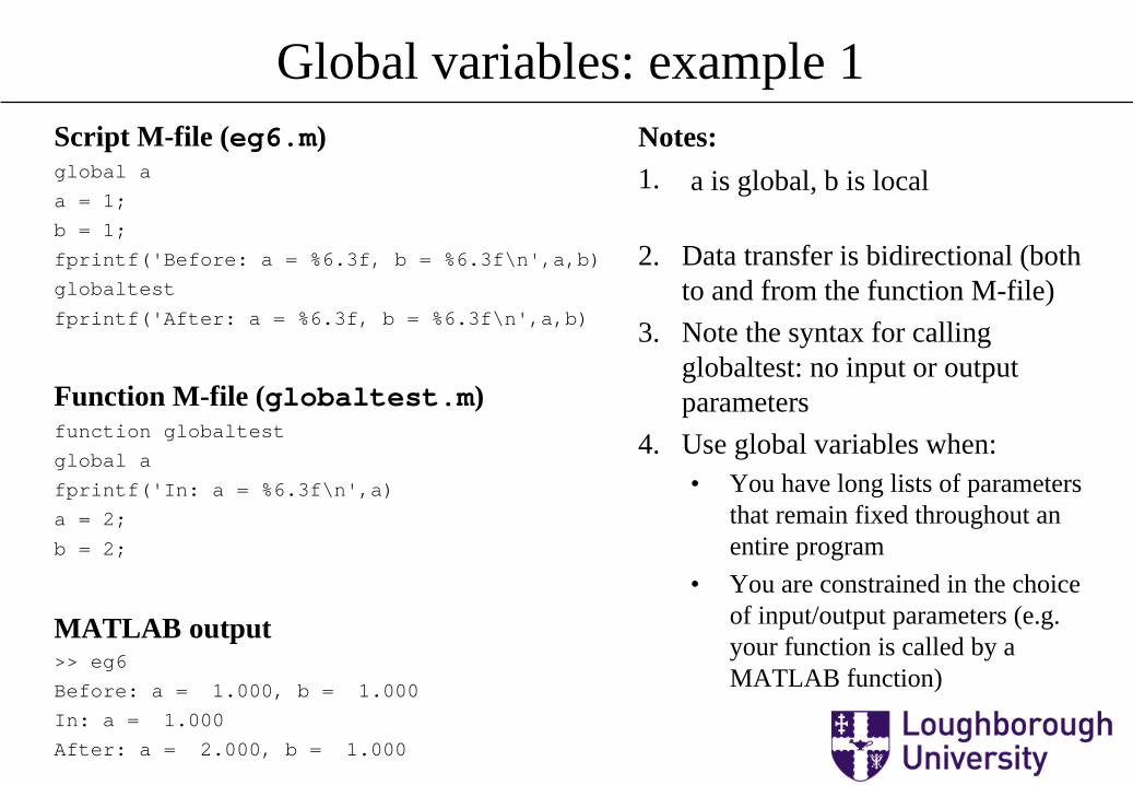
Global variables: example 1 Script M-file (eg6.m) global a

a = 1;

b = 1;

fprintf('Before: a = %6.3f, b = %6.3f\n',a,b)

globaltest

fprintf('After: a = %6.3f, b = %6.3f\n',a,b)

Function M-file (globaltest.m) function globaltest

global a

fprintf('In: a = %6.3f\n',a)

a = 2;

b = 2;

MATLAB output >> eg6

Before: a = 1.000, b = 1.000

In: a = 1.000

After: a = 2.000, b = 1.000

Notes: 1.

2. Data transfer is bidirectional (both

to and from the function M-file) 3. Note the syntax for calling

globaltest: no input or output parameters

4. Use global variables when: • You have long lists of parameters

that remain fixed throughout an entire program

• You are constrained in the choice of input/output parameters (e.g. your function is called by a MATLAB function)

a is global, b is local

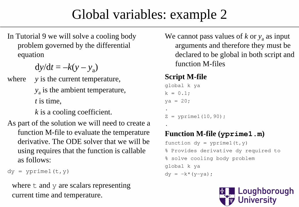
Global variables: example 2 In Tutorial 9 we will solve a cooling body

problem governed by the differential equation

dy/dt = –k(y – ya) where y is the current temperature, ya is the ambient temperature, t is time, k is a cooling coefficient. As part of the solution we will need to create a

function M-file to evaluate the temperature derivative. The ODE solver that we will be using requires that the function is callable as follows:

dy = yprime1(t,y)

We cannot pass values of k or ya as input arguments and therefore they must be declared to be global in both script and function M-files

Script M-file global k ya

k = 0.1;

ya = 20;

.

Z = yprime1(10,90);

.

Function M-file (yprime1.m) function dy = yprime1(t,y)

% Provides derivative dy required to

% solve cooling body problem

global k ya

dy = -k*(y-ya);

where t and y are scalars representing current time and temperature.

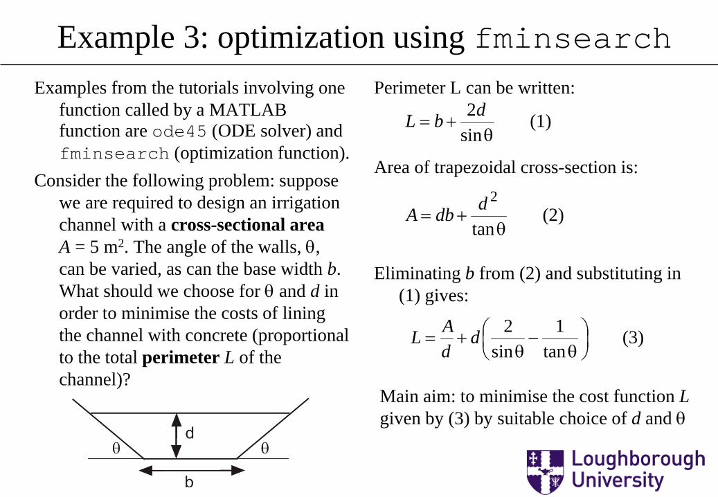
Example 3: optimization using fminsearch Examples from the tutorials involving one

function called by a MATLAB function are ode45 (ODE solver) and fminsearch (optimization function).

Consider the following problem: suppose we are required to design an irrigation channel with a cross-sectional area A = 5 m2. The angle of the walls, θ, can be varied, as can the base width b. What should we choose for θ and d in order to minimise the costs of lining the channel with concrete (proportional to the total perimeter L of the channel)?

Perimeter L can be written: Area of trapezoidal cross-section is: Eliminating b from (2) and substituting in

(1) gives:

(1) sin2

θ+=

dbL

(2) tan

2

θ+=

ddbA

(3) tan

1sin

2

θ−

θ+= d

dAL

Main aim: to minimise the cost function L given by (3) by suitable choice of d and θ

Function M-file called by fminsearch This is an example of a non-linear multi-dimensional (in this case 2-D) optimisation

(minimisation) problem. The MATLAB optimisation toolbox has a range of functions to solve problems of this type. The relevant function in this case is

xo = fminsearch(fun,xi) where xi is an initial estimate of the solution (a row vector with a value for each

variable being optimised – in this case, 2), xo is the optimised solution vector , fun is the name of a user-supplied function to evaluate the cost function, callable as cost = fun(x) and where cost is the value of the cost (a scalar) evaluated at vector x. Suitable function M-file (channel.m) for the channel problem function L = channel(x) % Returns perimeter L for a channel % Input parameters: x(1) = channel depth (d) % : x(2) = wall angle (theta) % Requires cross-sectional area A to be defined as % global in main script M-file global A L = A/x(1) + x(1)*(2/sin(x(2)) - 1/tan(x(2)));

fminsearch: example script M-file and output Script M-file (channeloptimise.m) % Script M-file to optimise the design of irrigation channel

global A

A = 5; % require cross-section of 5m^2

xi = [1 pi/2]; % initial guess for d and theta

xo = fminsearch('channel',xi); % optimised solution for d and theta

Li = channel(xi); % channel perimeter using initial guess

Lo = channel(xo); % channel perimeter using optimised solution

fprintf(' Perimeter = %6.3f with initial guess: d = %6.3f m, theta = %6.3f\n',Li,xi)

fprintf(' Perimeter = %6.3f with optimised solution: d = %6.3f m, theta = %6.3f\n',Lo,xo)

MATLAB output >>channeloptimise

Perimeter = 7.000 with initial guess: d = 1.000 m, theta = 1.571

Perimeter = 5.886 with optimised solution: d = 1.699 m, theta = 1.047

Important point:

Non-linear optimisations can find the wrong solution (a local minimum of the cost function) if the initial estimate is too far from the global minimum.