ME346A Introduction to Statistical Mechanics – Wei Cai – Stanford University – Win 2011

Handout 12. Ising Model

February 25, 2011

Contents

1 Definition of Ising model 2

2 Solving the 1D Ising model 42.1 Non-interacting model (J = 0) . . . . . . . . . . . . . . . . . . . . . . . . . . 42.2 Ising model at zero field (h = 0) . . . . . . . . . . . . . . . . . . . . . . . . . 52.3 The general case (J 6= 0, h 6= 0) . . . . . . . . . . . . . . . . . . . . . . . . . 7

3 Generalized 1D Ising model 113.1 Spins with more than two states . . . . . . . . . . . . . . . . . . . . . . . . . 113.2 More than one row of spins . . . . . . . . . . . . . . . . . . . . . . . . . . . 12

4 2D Ising model 134.1 Analytic solution . . . . . . . . . . . . . . . . . . . . . . . . . . . . . . . . . 134.2 Monte Carlo simulation . . . . . . . . . . . . . . . . . . . . . . . . . . . . . . 144.3 Qualitative behavior . . . . . . . . . . . . . . . . . . . . . . . . . . . . . . . 174.4 Sketch of derivations of partition function in 2D . . . . . . . . . . . . . . . . 20

A major topic of interest in statistical mechanics (and in physics in general) is the under-standing of phase transitions (e.g. freezing of water to form ice), which requires the studyof interacting models.

The 2-dimensional (2D) Ising model (see front page image on coursework) is one of the fewinteracting models that have been solved analytically (by Onsager, who found the expressionof its partition function). It turns out that the 2D Ising model exhibits a phase transition.The analytic and numerical solutions of the Ising model are important landmarks in thefield of statistical mechanics. They have significantly influenced our understanding of phasetransitions.

We will first discuss the simpler 1-dimensional (1D) Ising model, whose analytic solution is

1

easier to obtain. This will pave the road to the discussion of the 2D Ising model which comesnext.

Reading assignment: Sethna p.163-165. Reif Chapter 10.

1 Definition of Ising model

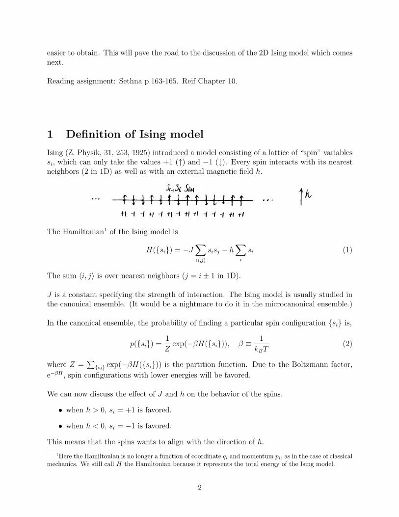
Ising (Z. Physik, 31, 253, 1925) introduced a model consisting of a lattice of “spin” variablessi, which can only take the values +1 (↑) and −1 (↓). Every spin interacts with its nearestneighbors (2 in 1D) as well as with an external magnetic field h.

The Hamiltonian1 of the Ising model is

H({si}) = −J∑〈i,j〉

sisj − h∑i

si (1)

The sum 〈i, j〉 is over nearest neighbors (j = i± 1 in 1D).

J is a constant specifying the strength of interaction. The Ising model is usually studied inthe canonical ensemble. (It would be a nightmare to do it in the microcanonical ensemble.)

In the canonical ensemble, the probability of finding a particular spin configuration {si} is,

p({si}) =1

Zexp(−βH({si})), β ≡ 1

kBT(2)

where Z =∑{si} exp(−βH({si})) is the partition function. Due to the Boltzmann factor,

e−βH , spin configurations with lower energies will be favored.

We can now discuss the effect of J and h on the behavior of the spins.

• when h > 0, si = +1 is favored.

• when h < 0, si = −1 is favored.

This means that the spins wants to align with the direction of h.

1Here the Hamiltonian is no longer a function of coordinate qi and momentum pi, as in the case of classicalmechanics. We still call H the Hamiltonian because it represents the total energy of the Ising model.

2

• when J > 0, neighboring spins prefer to be parallel, e.g. si = +1 and si+1 = +1, orsi = −1 and si+1 = −1. (This is called the ferromagnetic model.)

• when J < 0, neighboring spins prefer to be anti-parallel, e.g. si = +1 and si+1 = −1,or si = −1 and si+1 = +1. (This is called the anti-ferromagnetic model.)

At low enough temperature, all spins in the 2D Ising model will “cooperate” and sponta-neously align themselves (e.g. most spins become +1) even in the absence of the externalfield (h = 0). This phenomenon is called spontaneous magnetization.

At high enough temperatures, the spontaneous magnetization is destroyed by thermal fluc-tuation. Hence the 2D Ising model has a critical temperature Tc, below which there isspontaneous magnetization and above which there isn’t. In other words, there is a phasetransition at Tc.

Unfortunately this doesn’t occur in the 1D Ising model. The 1D Ising model does not havea phase transition. We are discussing it here just to “warm up” for the discussion of the 2DIsing model.

The term “spin” and “magnetic field” in the Ising model originate from its initial applicationto the phenomenon of spontaneous magnetization in ferromagnetic materials such as iron.Each iron atom has a unpaired electron and hence a net spin (or magnetic moment). At lowtemperature, the spins spontaneously align giving rise to a non-zero macroscopic magneticmoment. The macroscopic magnetic moment disappears when the temperature exceeds theCurie temperature (1043 K for iron). (See http://en.wikipedia.org/wiki/Ferromagneticfor more details.) As we will see later, the Ising model can be applied to many other problemsbeyond magnetism, such as phase separation in binary alloys and crystal growth.

3

2 Solving the 1D Ising model

Q: What do we mean by solving the Ising model?

A: We are really after the partition function Z, as a function of J and h. If we have theanalytic expression for Z, we can easily obtain all thermodynamic properties of theIsing model.

2.1 Non-interacting model (J = 0)

Let us first consider the simpler case of J = 0 (h 6= 0). This is a non-interacting model. Itis the same as the two-level systems we have considered in the canonical ensemble section!

Z =∑{si}

eβh∑i si =

∑{si}

N∏i=1

eβhsi =N∏i=1

∑{si=±1}

eβhsi

=(eβh + e−βh

)N= (2 cosh βh)N (3)

Q: What thermodynamic quantities are we interested in?

A: Helmholtz free energy A(N, T, h), energy E, entropy S, and average magnetization

M(N, T, h) ≡⟨∑N

i=1 si

⟩.

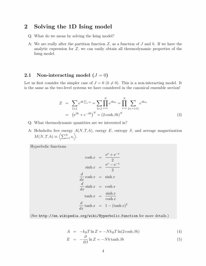
Hyperbolic functions

coshx =ex + e−x

2

sinhx =ex − e−x

2d

dxcoshx = sinhx

d

dxsinhx = coshx

tanhx =sinhx

coshxd

dxtanhx = 1− (tanhx)2

(See http://en.wikipedia.org/wiki/Hyperbolic function for more details.)

A = −kBT lnZ = −NkBT ln(2 cosh βh) (4)

E = − ∂

∂βlnZ = −Nh tanh βh (5)

4

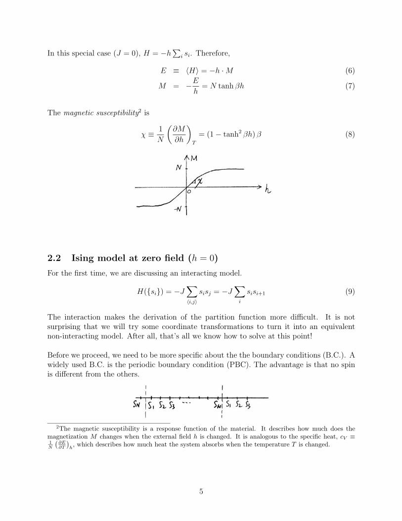
In this special case (J = 0), H = −h∑

i si. Therefore,

E ≡ 〈H〉 = −h ·M (6)

M = −Eh

= N tanh βh (7)

The magnetic susceptibility2 is

χ ≡ 1

N

(∂M

∂h

)T

= (1− tanh2 βh) β (8)

2.2 Ising model at zero field (h = 0)

For the first time, we are discussing an interacting model.

H({si}) = −J∑〈i,j〉

sisj = −J∑i

sisi+1 (9)

The interaction makes the derivation of the partition function more difficult. It is notsurprising that we will try some coordinate transformations to turn it into an equivalentnon-interacting model. After all, that’s all we know how to solve at this point!

Before we proceed, we need to be more specific about the the boundary conditions (B.C.). Awidely used B.C. is the periodic boundary condition (PBC). The advantage is that no spinis different from the others.

2The magnetic susceptibility is a response function of the material. It describes how much does themagnetization M changes when the external field h is changed. It is analogous to the specific heat, cV ≡1N

(∂E∂T

)h, which describes how much heat the system absorbs when the temperature T is changed.

5

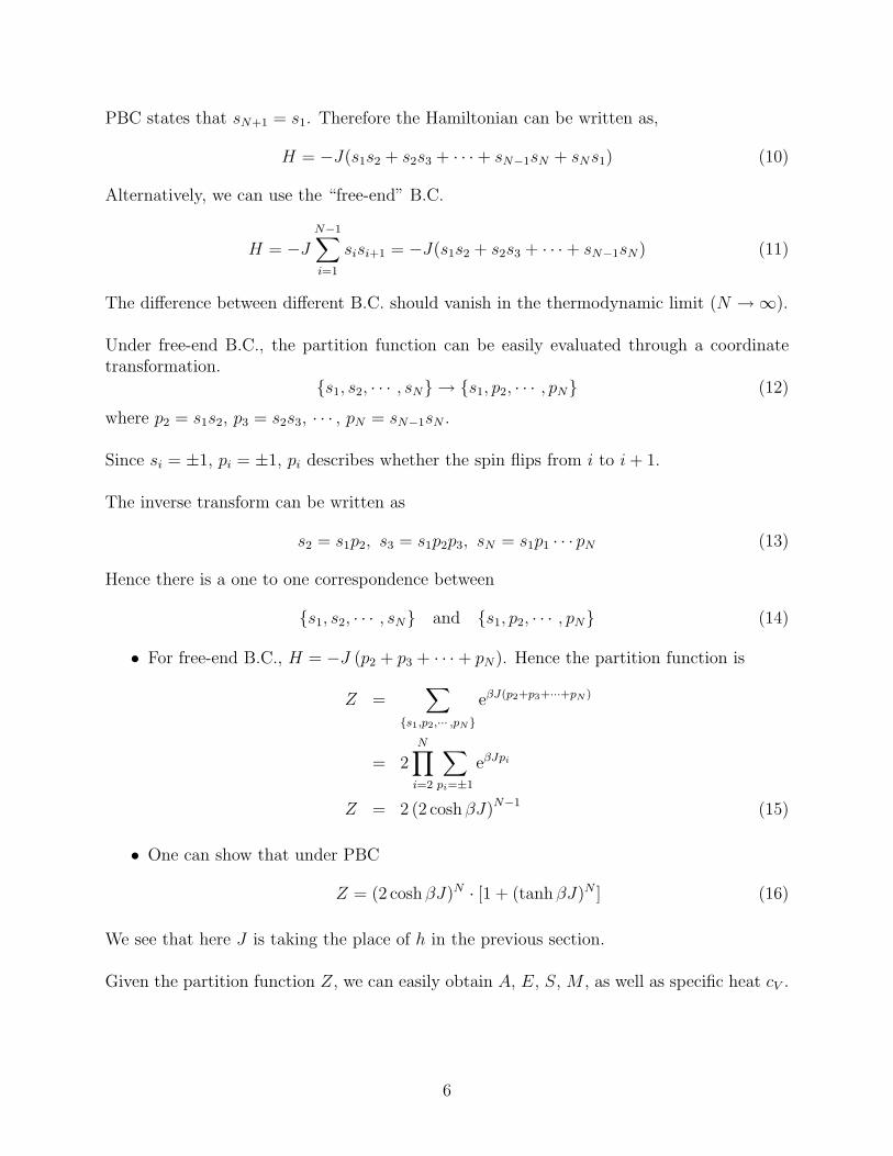
PBC states that sN+1 = s1. Therefore the Hamiltonian can be written as,

H = −J(s1s2 + s2s3 + · · ·+ sN−1sN + sNs1) (10)

Alternatively, we can use the “free-end” B.C.

H = −JN−1∑i=1

sisi+1 = −J(s1s2 + s2s3 + · · ·+ sN−1sN) (11)

The difference between different B.C. should vanish in the thermodynamic limit (N →∞).

Under free-end B.C., the partition function can be easily evaluated through a coordinatetransformation.

{s1, s2, · · · , sN} → {s1, p2, · · · , pN} (12)

where p2 = s1s2, p3 = s2s3, · · · , pN = sN−1sN .

Since si = ±1, pi = ±1, pi describes whether the spin flips from i to i+ 1.

The inverse transform can be written as

s2 = s1p2, s3 = s1p2p3, sN = s1p1 · · · pN (13)

Hence there is a one to one correspondence between

{s1, s2, · · · , sN} and {s1, p2, · · · , pN} (14)

• For free-end B.C., H = −J (p2 + p3 + · · ·+ pN). Hence the partition function is

Z =∑

{s1,p2,··· ,pN}

eβJ(p2+p3+···+pN )

= 2N∏i=2

∑pi=±1

eβJpi

Z = 2 (2 cosh βJ)N−1 (15)

• One can show that under PBC

Z = (2 cosh βJ)N · [1 + (tanh βJ)N ] (16)

We see that here J is taking the place of h in the previous section.

Given the partition function Z, we can easily obtain A, E, S, M , as well as specific heat cV .

6

2.3 The general case (J 6= 0, h 6= 0)

To obtain the magnetic susceptibility χ at non-zero J , we need to consider the case of J 6= 0,h 6= 0, which is a true interacting model.

The partition function is usually expressed in terms of the trace of a matrix.

The trace is the sum of the diagonal elements of a matrix

Tr(B) = B11 +B22 + · · ·+Bnn (17)

where B =

B11 B12 · · · B1n

B21 B22 · · · B2n...

.... . .

Bn1 Bn2 · · · Bnn

(18)

For example, for an Ising model with one spin, H = −h s1, the partition function is

Z = Tr

(eβh 00 e−βh

)= eβh + e−βh (19)

Now consider two spins, under periodic B.C.,

H(s1, s2) = −Js1s2 − Js2s1 − hs1 − hs2 (20)

Define matrix

P ≡(

eβ(J+h) e−βJ

e−βJ eβ(J−h)

)(21)

then,

Z =∑{s1s2}

e−βH = Tr(P · P ) (22)

Q: Why?

A: Notice that P is a 2× 2 matrix.

Let the 1st row (column) correspond to s = +1, and let the 2nd row(column) corre-spond to s = −1, e.g.,

P+1,+1 = eβ(J+h), P+1,−1 = e−β J ,

P−1,+1 = e−β J , P−1,−1 = eβ(J−h),

Ps1s2 = eβ(Js1s2+h2s1+h

2s2) (23)

Tr(P · P ) =∑s1

(P · P )s1,s1 =∑s1,s2

Ps1,s2 Ps2,s1 (24)

7

∴ Tr(P · P ) =∑s1,s2

eβ(Js1s2+h2s1+h

2s2) · eβ(Js2s1+h

2s2+h

2s1)

=∑s1,s2

e−βH(s1,s2)

= Z (25)

In general, for N spins forming a linear chain under PBC, the partition function is

Z =∑{si}

e−βH({si})

=∑{si}

eβ(Js1s2+h2s1+h

2s2) · eβ(Js2s3+h

2s2+h

2s3) · · ·

eβ(JsN−1sN+h2sN−1+h

2sN) · eβ(JsNs1+h

2sN+h

2s1)

= Tr(PN)

(26)

Now we have obtained a concise formal expression for the partition function. But to computematrix PN , it requires a lot of calculations. Fortunately, we don’t need PN . we just needTr(PN). This is the time we need to introduce a little more matrix theory, concerning theproperties of the trace.

1. Every symmetric (real) matrix can be diagonalized,

P = U ·D · UT (27)

where U is a unitary matrix (U ·UT = I), and D is a diagonal matrix. For 2×2matrices, define λ+ ≡ D11, λ− ≡ D22 (D12 = D21 = 0). λ± are the eigenvaluesof matrix P .

2. Trace is unchanged after diagonalization

Tr(P) = Tr(D) = λ+ + λ− (28)

Hence the trace equals the sum of the eigenvalues.

3. The same matrix U that diagonalizes P also diagonalizes PN , because

PN =(U ·D · UT

)·(U ·D · UT

)· · ·(U ·D · UT

)= U ·DN · UT (29)

4. Notice that

DN =

(λN+ 00 λN−

)(30)

We haveTr(PN) = Tr(DN) = λN+ + λN− (31)

8

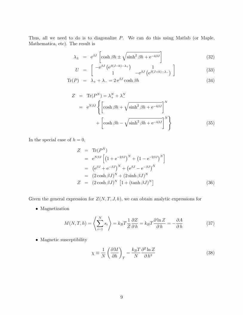
Thus, all we need to do is to diagonalize P . We can do this using Matlab (or Maple,Mathematica, etc). The result is

λ± = eβJ[cosh βh±

√sinh2 βh+ e−4βJ

](32)

U =

[−eβJ

(eβ(J−h)−λ+

)1

1 −eβJ(eβ(J+h)−λ−

) ] (33)

Tr(P ) = λ+ + λ− = 2 eβJ cosh βh (34)

Z = Tr(PN) = λN+ + λN−

= eNβJ

{[cosh βh+

√sinh2 βh+ e−4βJ

]N+

[cosh βh−

√sinh2 βh+ e−4βJ

]N}(35)

In the special case of h = 0,

Z = Tr(PN)

= eNβJ[(

1 + e−2βJ)N

+(1− e−2βJ

)N]=

(eβJ + e−βJ

)N+(eβJ − e−βJ

)N= (2 cosh βJ)N + (2 sinh βJ)N

Z = (2 cosh βJ)N[1 + (tanh βJ)N

](36)

Given the general expression for Z(N, T, J, h), we can obtain analytic expressions for

• Magnetization

M(N, T, h) =

⟨N∑i=1

si

⟩= kBT

1

Z

∂Z

∂ h= kBT

∂ lnZ

∂ h= −∂A

∂ h(37)

• Magnetic susceptibility

χ ≡ 1

N

(∂M

∂h

)T

=kBT

N

∂2 lnZ

∂ h2(38)

9

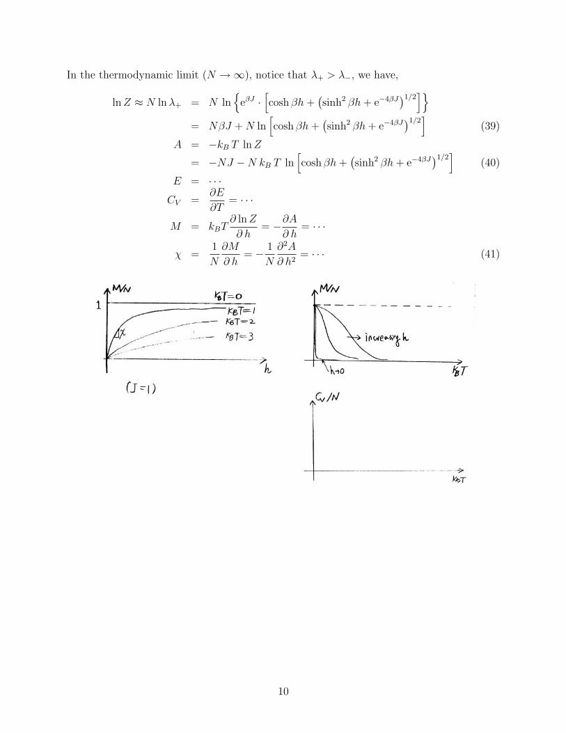
In the thermodynamic limit (N →∞), notice that λ+ > λ−, we have,

lnZ ≈ N lnλ+ = N ln{

eβJ ·[cosh βh+

(sinh2 βh+ e−4βJ

)1/2]}

= NβJ +N ln[cosh βh+

(sinh2 βh+ e−4βJ

)1/2]

(39)

A = −kB T lnZ

= −NJ −N kB T ln[cosh βh+

(sinh2 βh+ e−4βJ

)1/2]

(40)

E = · · ·CV =

∂E

∂T= · · ·

M = kBT∂ lnZ

∂ h= −∂A

∂ h= · · ·

χ =1

N

∂M

∂ h= − 1

N

∂2A

∂ h2= · · · (41)

10

3 Generalized 1D Ising model

3.1 Spins with more than two states

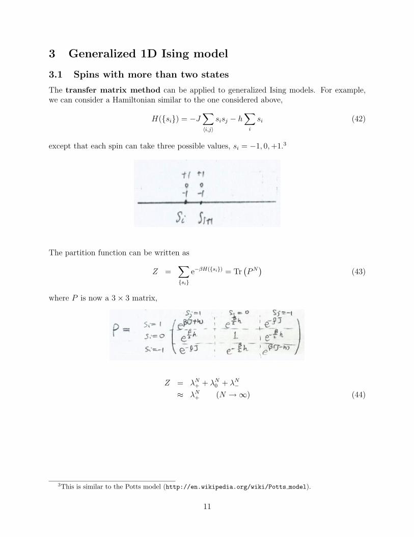
The transfer matrix method can be applied to generalized Ising models. For example,we can consider a Hamiltonian similar to the one considered above,

H({si}) = −J∑〈i,j〉

sisj − h∑i

si (42)

except that each spin can take three possible values, si = −1, 0,+1.3

The partition function can be written as

Z =∑{si}

e−βH({si}) = Tr(PN)

(43)

where P is now a 3× 3 matrix,

Z = λN+ + λN0 + λN−≈ λN+ (N →∞) (44)

3This is similar to the Potts model (http://en.wikipedia.org/wiki/Potts model).

11

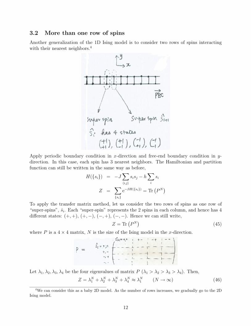
3.2 More than one row of spins

Another generalization of the 1D Ising model is to consider two rows of spins interactingwith their nearest neighbors.4

Apply periodic boundary condition in x-direction and free-end boundary condition in y-direction. In this case, each spin has 3 nearest neighbors. The Hamiltonian and partitionfunction can still be written in the same way as before,

H({si}) = −J∑〈i,j〉

sisj − h∑i

si

Z =∑{si}

e−βH({si}) = Tr(PN)

To apply the transfer matrix method, let us consider the two rows of spins as one row of“super-spins”, si. Each “super-spin” represents the 2 spins in each column, and hence has 4different states: (+,+), (+,−), (−,+), (−,−). Hence we can still write,

Z = Tr(PN)

(45)

where P is a 4× 4 matrix, N is the size of the Ising model in the x-direction.

Let λ1, λ2, λ3, λ4 be the four eigenvalues of matrix P (λ1 > λ2 > λ3 > λ4). Then,

Z = λN1 + λN2 + λN3 + λN4 ≈ λN1 (N →∞) (46)

4We can consider this as a baby 2D model. As the number of rows increases, we gradually go to the 2DIsing model.

12

4 2D Ising model

4.1 Analytic solution

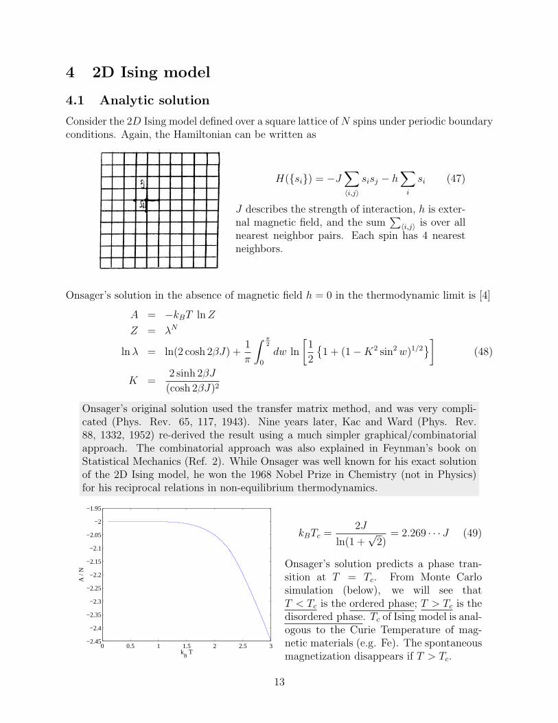
Consider the 2D Ising model defined over a square lattice of N spins under periodic boundaryconditions. Again, the Hamiltonian can be written as

H({si}) = −J∑〈i,j〉

sisj − h∑i

si (47)

J describes the strength of interaction, h is exter-nal magnetic field, and the sum

∑〈i,j〉 is over all

nearest neighbor pairs. Each spin has 4 nearestneighbors.

Onsager’s solution in the absence of magnetic field h = 0 in the thermodynamic limit is [4]

A = −kBT lnZ

Z = λN

lnλ = ln(2 cosh 2βJ) +1

π

∫ π2

0

dw ln

[1

2

{1 + (1−K2 sin2w)1/2

}](48)

K =2 sinh 2βJ

(cosh 2βJ)2

Onsager’s original solution used the transfer matrix method, and was very compli-cated (Phys. Rev. 65, 117, 1943). Nine years later, Kac and Ward (Phys. Rev.88, 1332, 1952) re-derived the result using a much simpler graphical/combinatorialapproach. The combinatorial approach was also explained in Feynman’s book onStatistical Mechanics (Ref. 2). While Onsager was well known for his exact solutionof the 2D Ising model, he won the 1968 Nobel Prize in Chemistry (not in Physics)for his reciprocal relations in non-equilibrium thermodynamics.

0 0.5 1 1.5 2 2.5 3−2.45

−2.4

−2.35

−2.3

−2.25

−2.2

−2.15

−2.1

−2.05

−2

−1.95

kB T

A /

N

kBTc =2J

ln(1 +√

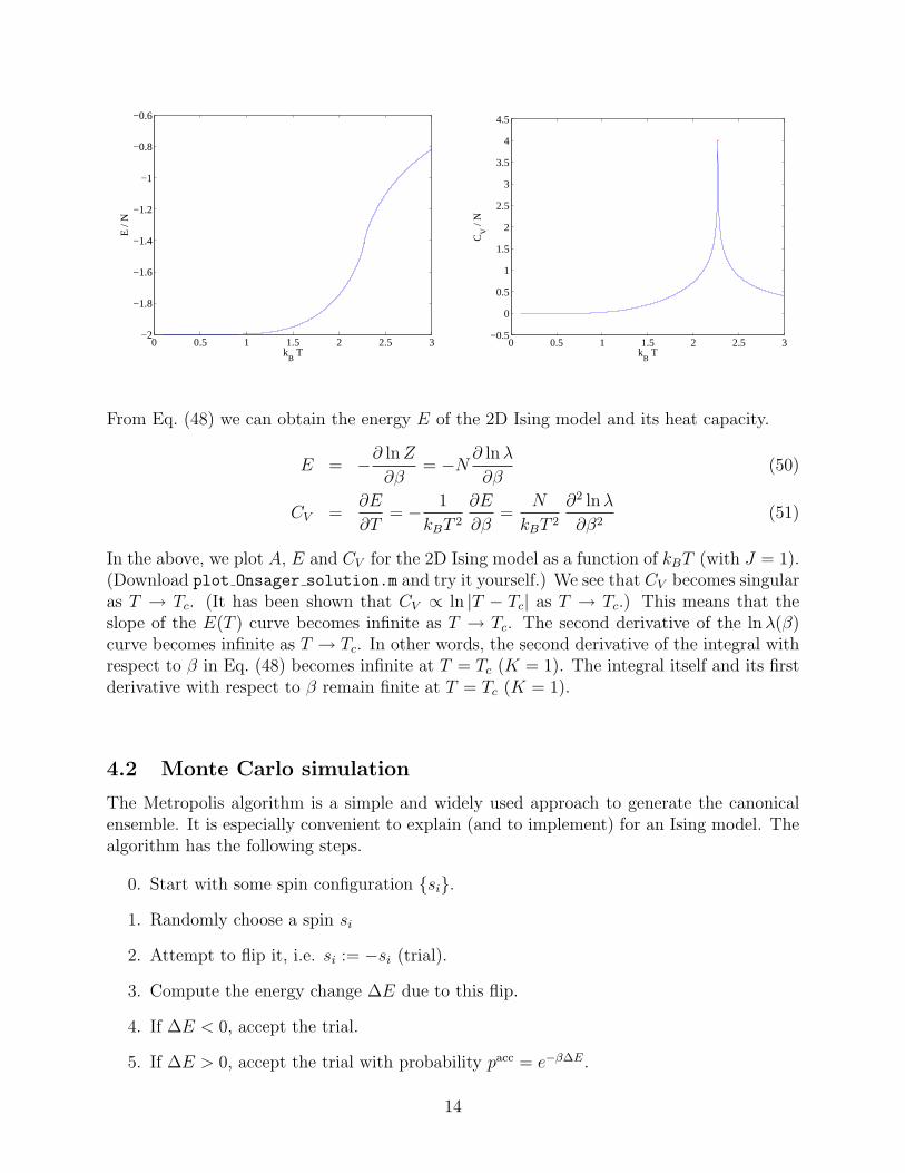
2)= 2.269 · · · J (49)

Onsager’s solution predicts a phase tran-sition at T = Tc. From Monte Carlosimulation (below), we will see thatT < Tc is the ordered phase; T > Tc is thedisordered phase. Tc of Ising model is anal-ogous to the Curie Temperature of mag-netic materials (e.g. Fe). The spontaneousmagnetization disappears if T > Tc.

13

0 0.5 1 1.5 2 2.5 3−2

−1.8

−1.6

−1.4

−1.2

−1

−0.8

−0.6

kB T

E /

N

0 0.5 1 1.5 2 2.5 3−0.5

0

0.5

1

1.5

2

2.5

3

3.5

4

4.5

kB T

CV /

N

From Eq. (48) we can obtain the energy E of the 2D Ising model and its heat capacity.

E = −∂ lnZ

∂β= −N ∂ lnλ

∂β(50)

CV =∂E

∂T= − 1

kBT 2

∂E

∂β=

N

kBT 2

∂2 lnλ

∂β2(51)

In the above, we plot A, E and CV for the 2D Ising model as a function of kBT (with J = 1).(Download plot Onsager solution.m and try it yourself.) We see that CV becomes singularas T → Tc. (It has been shown that CV ∝ ln |T − Tc| as T → Tc.) This means that theslope of the E(T ) curve becomes infinite as T → Tc. The second derivative of the lnλ(β)curve becomes infinite as T → Tc. In other words, the second derivative of the integral withrespect to β in Eq. (48) becomes infinite at T = Tc (K = 1). The integral itself and its firstderivative with respect to β remain finite at T = Tc (K = 1).

4.2 Monte Carlo simulation

The Metropolis algorithm is a simple and widely used approach to generate the canonicalensemble. It is especially convenient to explain (and to implement) for an Ising model. Thealgorithm has the following steps.

0. Start with some spin configuration {si}.

1. Randomly choose a spin si

2. Attempt to flip it, i.e. si := −si (trial).

3. Compute the energy change ∆E due to this flip.

4. If ∆E < 0, accept the trial.

5. If ∆E > 0, accept the trial with probability pacc = e−β∆E.

14

6. If trial is rejected, put the spin back, i.e. si := −si.

7. Go to 1, unless maximum number of iterations is reached.

* More details about this algorithm will be discussed later.

Numerical exercise: run ising2d.m for N = 80×80, starting from random initial conditions,with J = 1, at kBT = 0.5, 1, 1.5, 2, 2.269, 3. Write down your observations.

kBT = 0.5 kBT = 2.269 kBT = 3

Q: Why does the Metropolis algorithm generate the canonical distribution?

To simplify the notation, let A, B represent arbitrary spin configurations {si}. Our goal isto prove that when the MC simulation has reached equilibrium, the probability of samplingstate A is

pA =1

Ze−βH(A) (52)

whereZ =

∑A

e−βH(A) (53)

— the sum is over all possible (2N) spin configurations.

Monte Carlo simulation follows a Markov Chain, which is completely specified by a transitionprobability matrix πAB — the probability of jumping to state B in the next step if the currentstate is A.

For an Ising model with N spins, there are 2N spin configurations (states). So πAB is a2N × 2N matrix. However, most entries in πAB are zeros.

πAB 6= 0 only if there is no more than one spin that is different (flipped) between A and B.For example,

if A = {+1,+1,+1,+1,+1,+1} then

for B = {+1,−1,+1,+1,+1,+1}, πAB > 0

but for B = {−1,−1,+1,+1,+1,+1}, πAB = 0

15

To prove the Metropolis algorithm generates the canonical ensemble:

(1) transition matrix can be written as

πAB = αAB · paccAB, for B 6= A (54)

πAA = 1−∑B 6=A

πAB (55)

where αAB is the trial probability that satisfies

αAB = αBA (56)

and paccAB is the acceptance probability.

without loss of generality, let’s assume EB > EA, then{paccAB = exp

(−EB−EA

kBT

)paccBA = 1

=⇒ πABπBA

=αABαBA

paccABpaccBA

= exp

(−EB − EA

kBT

)(57)

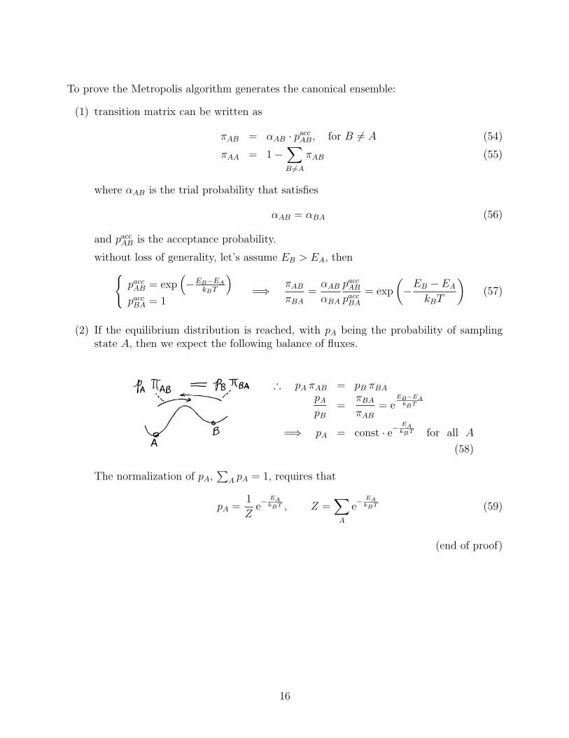
(2) If the equilibrium distribution is reached, with pA being the probability of samplingstate A, then we expect the following balance of fluxes.

∴ pA πAB = pB πBApApB

=πBAπAB

= eEB−EAkBT

=⇒ pA = const · e−EAkBT for all A

(58)

The normalization of pA,∑

A pA = 1, requires that

pA =1

Ze− EAkBT , Z =

∑A

e− EAkBT (59)

(end of proof)

16

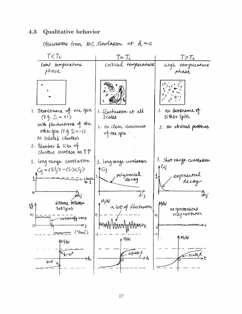
4.3 Qualitative behavior

17

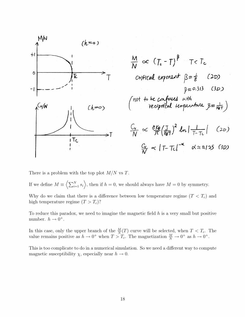
There is a problem with the top plot M/N vs T .

If we define M ≡⟨∑N

i=1 si

⟩, then if h = 0, we should always have M = 0 by symmetry.

Why do we claim that there is a difference between low temperature regime (T < Tc) andhigh temperature regime (T > Tc)?

To reduce this paradox, we need to imagine the magnetic field h is a very small but positivenumber. h→ 0+.

In this case, only the upper branch of the MN

(T ) curve will be selected, when T < Tc. Thevalue remains positive as h→ 0+ when T > Tc. The magnetization M

N→ 0+ as h→ 0+.

This is too complicate to do in a numerical simulation. So we need a different way to computemagnetic susceptibility χ, especially near h→ 0.

18

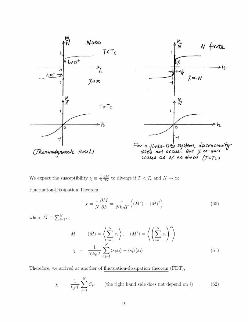
We expect the susceptibility χ ≡ 1N∂M∂N

to diverge if T < Tc and N →∞.

Fluctuation-Dissipation Theorem

χ =1

N

∂M

∂h=

1

NkBT

(〈M2〉 − 〈M〉2

)(60)

where M ≡∑N

i=1 si

M ≡ 〈M〉 =

⟨N∑i=1

si

⟩, 〈M2〉 =

⟨(N∑i=1

si

)2⟩.

χ =1

NkBT

N∑i,j=1

〈sisj〉 − 〈si〉〈sj〉 (61)

Therefore, we arrived at another of fluctuation-dissipation theorem (FDT),

χ =1

kBT

N∑j=1

Cij (the right hand side does not depend on i) (62)

19

whereCij ≡ 〈sisj〉 − 〈si〉〈sj〉 (63)

is the correlation function between spins i and j. When T < Tc, χ → ∞, corresponding tolong range correlation,

∑Nj=1Cij ∝ N . (unbounded as N →∞).

Proof of Eq. (60)

Z =∑{si}

e−βH({si}) =∑{si}

exp

βJ∑〈i,j〉

sisj + βh∑i

si

∂Z

∂h=

∑{si}

e−βH({si}) β M (64)

M = kBT1

Z

∂Z

∂h(65)

∂M

∂h= kBT

[1

Z

∂2Z

∂h2− 1

Z2

(∂Z

∂h

)2]

= kBT[β2〈M2〉 − β2〈M〉2

]=

1

kBT

[〈M2〉 − 〈M〉2

](66)

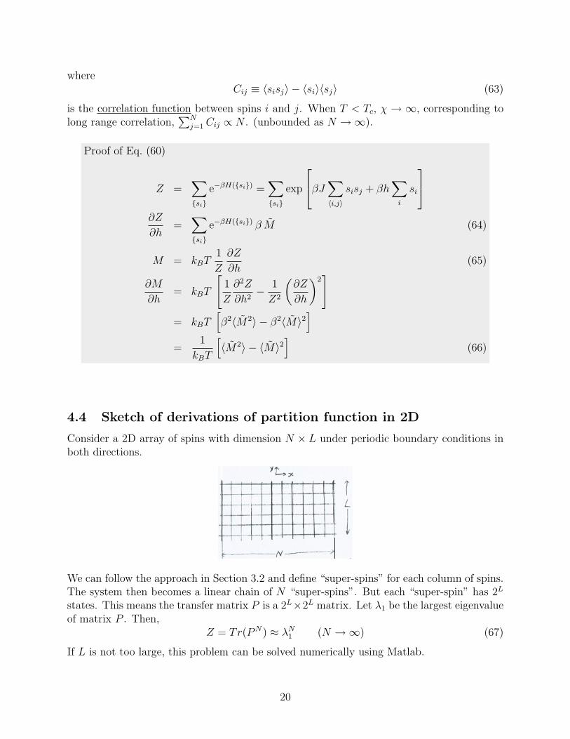
4.4 Sketch of derivations of partition function in 2D

Consider a 2D array of spins with dimension N × L under periodic boundary conditions inboth directions.

We can follow the approach in Section 3.2 and define “super-spins” for each column of spins.The system then becomes a linear chain of N “super-spins”. But each “super-spin” has 2L

states. This means the transfer matrix P is a 2L×2L matrix. Let λ1 be the largest eigenvalueof matrix P . Then,

Z = Tr(PN) ≈ λN1 (N →∞) (67)

If L is not too large, this problem can be solved numerically using Matlab.

20

This is the approach Onsager took (1943) to find the analytic solution for Z in the limit ofN →∞, L→∞.5

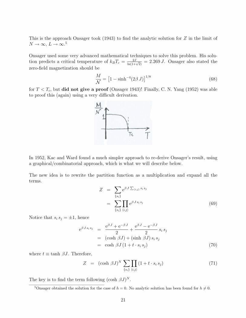
Onsager used some very advanced mathematical techniques to solve this problem. His solu-tion predicts a critical temperature of kBTc = 2J

ln(1+√

2)= 2.269 J . Onsager also stated the

zero-field magnetization should be

M

N=[1− sinh−4(2β J)

]1/8(68)

for T < Tc, but did not give a proof (Onsager 1943)! Finally, C. N. Yang (1952) was ableto proof this (again) using a very difficult derivation.

In 1952, Kac and Ward found a much simpler approach to re-derive Onsager’s result, usinga graphical/combinatorial approach, which is what we will describe below.

The new idea is to rewrite the partition function as a multiplication and expand all theterms.

Z =∑{si}

eβ J∑〈i,j〉 si sj

=∑{si}

∏〈i,j〉

eβ J si sj (69)

Notice that si sj = ±1, hence

eβ J si sj =eβ J + e−β J

2+

eβ J − e−β J

2si sj

= (cosh βJ) + (sinh βJ) si sj

= cosh βJ (1 + t · si sj) (70)

where t ≡ tanh βJ . Therefore,

Z = (cosh βJ)N∑{si}

∏〈i,j〉

(1 + t · si sj) (71)

The key is to find the term following (cosh βJ)N .

5Onsager obtained the solution for the case of h = 0. No analytic solution has been found for h 6= 0.

21

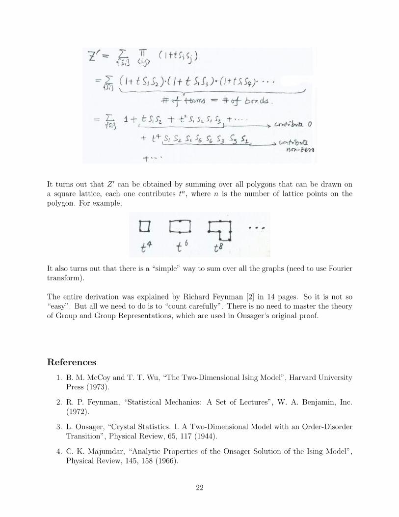
It turns out that Z ′ can be obtained by summing over all polygons that can be drawn ona square lattice, each one contributes tn, where n is the number of lattice points on thepolygon. For example,

It also turns out that there is a “simple” way to sum over all the graphs (need to use Fouriertransform).

The entire derivation was explained by Richard Feynman [2] in 14 pages. So it is not so“easy”. But all we need to do is to “count carefully”. There is no need to master the theoryof Group and Group Representations, which are used in Onsager’s original proof.

References

1. B. M. McCoy and T. T. Wu, “The Two-Dimensional Ising Model”, Harvard UniversityPress (1973).

2. R. P. Feynman, “Statistical Mechanics: A Set of Lectures”, W. A. Benjamin, Inc.(1972).

3. L. Onsager, “Crystal Statistics. I. A Two-Dimensional Model with an Order-DisorderTransition”, Physical Review, 65, 117 (1944).

4. C. K. Majumdar, “Analytic Properties of the Onsager Solution of the Ising Model”,Physical Review, 145, 158 (1966).

22