i

HANDOFFS IN HIERARCHICAL MACRO/FEMTO NETWORKS AND AN

ALGORITHM FOR EFFICIENT HANDOFFS

A THESIS SUBMITTED IN PARTIAL FULLFILLMENT OF THE REQUIREMENTS

FOR THE DEGREE OF

MASTERS IN TECHNOLOGY

IN

COMMUNICATION AND SIGNAL PROCESSING

BY

ABHISHEK MITRA

ROLL NO. 211EC4106

UNDER THE GUIDANCE OF

PROFESSOR SARAT KUMAR PATRA

DEPARTMENT OF ELECTRONICS AND COMMUNICATION ENGINEERING

NATIONAL INSTITUTE OF TECHNOLOGY ROURKELA, ROURKELA, ODISHA,

INDIA- 769008

May, 2014

ii

Certificate

This is to certify that the work in the thesis entitled “HANDOFFS IN HIERARCHICAL

MACRO/FEMTO NETWORKS AND AN ALGORITHM FOR EFFICIENT HANDOFFS”

by Abhishek Mitra is a record of an original research work carried out by him during 2013 -

2014 under my supervision and guidance in partial fulfillment of the requirements for the

award of the degree of Master of Technology in Electronics and Communication Engineering

(Communication and Networks), National Institute of Technology, Rourkela. Neither this

thesis nor any part of it, to the best of my knowledge, has been submitted for any degree or

diploma elsewhere.

Place: NIT Rourkela Dr. Sarat Kumar Patra

Professor,

Department of Electronics and

Communication, NIT Rourkela

Date: 2nd

june 2014

iii

ACKNOWLEDGEMENTS.

It would not have been possible to complete and write this project thesis without the help and

encouragement of certain people whom I would like to deeply honour and value their

gratefulness.

I would like to express my sincere gratitude to my supervisor and guide, Prof. Sarat Kumar

Patra. I highly honour the constant motivation and encouragement shown by him during the

project and writing of the thesis. Without his guidance and help, it would not have been

possible to bring out this thesis and complete the project.

My special thank goes to Prof. S.K.Meher Head of the Department of Electronics and

Communication Engineering, NIT, Rourkela, for providing us with best facilities in the

Department and his timely suggestions.

I am also thankful to other faculty and staff of Electronics and Communication department

for their support.

I would like show my gratitude to all the members of Mobile Communication Lab for their

constant support and co-operation throughout the course of the project. I would also like to

thank all my friends within and outside the department for all their encouragement,

motivation and the experiences that they shared with me.

Finally, I am deeply indebted to my parents who always had their belief in me and gave all

their support for all the choices that I have made.

ABHISHEK MITRA

iv

ABSTRACT.

The surest way to increase the system capacity of a wireless link is by getting the transmitter

and receiver closer to each other, which creates the dual benefits of higher-quality links and

more spatial reuse. In a network with nomadic users, this inevitably involves deploying more

infrastructure, typically in the form of microcells, hot spots, distributed antennas, or relays. A

less expensive alternative is the recent concept of femtocells also called home base stations

which are data access points installed by home users to get better indoor voice and data

coverage.

In macro/femto hierarchical networks, one of the biggest challenges is ensuring efficient

handoffs. Here in this thesis, we first evaluated received signal strength at mobile user using

different path loss models (indoor and outdoor) which is the main criterion for performing

handoff. We also obtained the interference and SINR scenarios for handoff performance.

Then we derived some basic handoff parameters like handoff probability, radio link failure

rate, ping-pong handoff for macro/femto environment. Finally we proposed an algorithm for

efficient handoff. The main idea of the proposed algorithm is to combine the values of

received signal strength from a serving macro BS and a target femto BS in the consideration

of large asymmetry in their transmit powers. Numerical results show that there is a significant

gain in view of the probability that the user will be assigned to the femtocell while keeping

the same level of the number of handoffs.

v

Contents.

Certificate

Acknowledgement

Abstract

List of figures

List of tables

List of abbreviations

1. Introduction………………………………...……………………………………..1

1.1. Background………………………….………………………………………1

1.2. Contribution…………………………………………………………………1

1.3.Thesis organisation………………………………………………………….2

2. Femto cell………………………………………………………………………..3

2.1.What is femtocell…………………………………………………………….4

2.2. Benefits of femtocell………………………………………………………...5

2.3.Femtocell network architecture………………………………………………6

2.4.Other small cell networks…………………………………………………….7

2.5.Femtocell vs. Wi-Fi…………………………………………………………..9

2.6.Challenges in femtocell………………………………………………………10

2.7.Accessing modes………………………………..…………………………..11

vi

3. Handoff……………………………………………………………………………12

3.1.Handoff………………………...……………………………………………….13

3.2.Types of handoff…………………………..……………………………………13

3.3.Handoff performance metrics……………………..……………………………14

3.4.Handoff procedure in femto cell…………………..……………………………14

3.5.Temporary femtocell visitor………………………...…………………………..15

3.6.Time to trigger……………………………………..……………………………16

3.7.SINR criterion…………………………………….…………………………….16

3.8.User state algorithm…………………………………………………………….17

4. Femtocell performance evaluation…………………………………………………18

4.1.Path loss models………………………………………………………………..19

4.2.Outdoor path loss models………………………………………………………19

4.3.Indoor path loss models………………………………………………………..20

4.4.Outdoor to indoor path loss models……………………………………………21

4.5.Capacity calculation in femtocell………………………………………………21

4.6.Channel model………………………………………………………………….22

4.7.Values of different parameters………………………………………………….23

4.8.Simulation results……………………………………………………………….24

4.9.Femtocell interference…………………………………...……………………..27

5. Handoff probabilities and failures…………………………………………………..33

5.1.Handoff probabilities and call arrival rate………………………………………34

5.2.Handover failures……………………………………………………………….37

5.3.Handover latency………………………………………………………………..41

6. Proposed algorithm………………………………………………………………….42

6.1.Mathematics of the algorithm…………………………………………………...45

vii

6.2.Handoff criterion for the algorithm……………………………………………...45

6.3.Performance analysis…………………………………………………………….46

6.4.Results and discussion……………………………………………………………46

7. Concluding remarks………………………………………………………………….49

7.1.Conclusion……………………………………………………………………….50

7.2.Bibliography……………………………………………………………………..52

viii

List of Figures.

Figure 2.1. Femtocell architecture…………………………………..……………………4

Figure 2.2 : Dense femtocellular network deployment scenario…………..……………..5

Figure 2.3 :Device to CN connectivity for femto cell deployment………..….………….7

Figure 2.4. DistributedAntennas…………….…………………………….…………….7

Fig 2.5. Micro cells……………………….………………………….…………………..8

Figure 4.1. Received power from femtocell with distance…………..……..…………..24

Figure 4.2. Received power from macrocell with distance………..…….……..……….25

Figure 4.3. SINR from macrocell/femtocell with distance……….…….…..…………..26

Figure 4.4. Throughput from macrocell/femtocell with distance………………………27

Figure 4.5. Serving and interfering FMC and path of the user…………………………28

Figure 4.6. Interference with no. of femtocells…………………………………………30

Figure 4.7. SINR with no. of femtocells………………………………………………..31

Figure 4.8. Probability of connection with no. of femtocells…………………………...32

Figure 5.1. Handoff probabilities with no. of femtocellls………………………………36

Figure 5.2. Too early handover and too late handover………………………………….37

Figure 5.3: Effect of handover margins on radio link failures due to too early and too late

handover…………………………………………………………...……………………38

Figure 5.4. RLF rate with hysteresis for different UE speed……………………………39

Figure 5.5. Ping-Pong rate with hysteresis for different UE speed……………………..40

ix

Figure 5.6. Handover latency with UE velocity………..……………..………………41

Fig 6.1 : Handoff scenario of MS moving from macrocell to femtocell……....……..44

Figure 6.2. Mobile user at macrocell/femtocell boundary scenario…………………...44

Figure 6.3. Optimal multiplying factor vs. distance of femto-macro BS……………...47

Figure 6.4.Assignment probability to femto BS vs. distance of macro-femto BS…......47

Figure 6.5. Number of handoffs vs. distance of macro-femto BS…………...…....…...48

x

List of Tables.

Table 2.1. Femtocells vs. Wi-Fi………………………………………………………9

Table 4.1. Simulation parameters for macrocell/femtocell handoff………………….23

xi

List of Abbreviations.

3GPP 3rd

Generation Partnership Project

AE Antenna Element

BS Base Station

CDMA Code division Multiple Access

CN Core network

DSL Digital subscriber line

FAP Femtocell Access Point

FBS Femto Base Station

FGW Femtocell gateway

FMC Fixed Mobile Convergence

GSM Global system for Mobile Communication

HeNB Home E-UTRAN Node B

HM Handover margin

ISP Internet service provider

LHO/EHO Too late handover/Too early handover

LOS Line of sight

LTE Long Term Evolution

MBS Macro Base Station

MS Mobile Station

OFDM Orthogonal Frequency Division Multiplexing

xii

QoS Quality of services

RB Resource block

RLF Radio link failure

RNC Radio network controller

RSS Received signal Strength

SON Self organising network

SINR Signal to Interference plus noise ratio

TTT Time to trigger

UE User Equipment

UL/DL Uplink/Downlink

WCDMA Wideband Code Division Multiple access

Wi-Fi Wireless Fidelity

Wi-MAX Worldwide interoperability for Microwave access

xiii

Chapter 1.

Introduction.

1

Introduction.

The best way to increase the system capacity of a wireless link is by getting the transmitter

and receiver closer to each other, which creates the dual benefits of higher-quality links and

more spatial reuse. In a network with nomadic users, this inevitably involves deploying more

infrastructure, typically in the form of microcells, hot spots, distributed antennas, or relays. A

less expensive alternative is the recent concept of femtocells — also called home base

stations — which are data access points installed by home users to get better indoor voice and

data coverage.

1.1.Background.

The concept of a compact self-optimising home cellsite has been documented since 1999.

Alcatel announced in March 1999 that they would bring to market a GSM home basestation

which would be compatible with existing standard GSM phones. They planned to launch the

product in 2000 and forecast capturing 50% of the market of 120 million units the following

year.

The system design re-used and modified the Cordless Telephony Standard (as used by

digital DECT cordless phones), which was a forerunner of the UMA standard used in dual-

mode WiFi/Cellular solutions today.

But now Femtocell technology has emerged as a most promising technology for home

environments. It gives high coverage and capacity as well as it is very cost effective. Now

various researches are going on for its better performance such as interference mitigation

from macro cell, proper spectrum allocation etc.

1.2.Contribution.

Here we concentrated on one the most important issues of femto cell performance i.e.

handoff from macrocell. First using different indoor and outdoor path loss models

received power and SINR from femtocell and macrocell are evaluated which are two

main criterion for handoff. Then various handover parameters are optimised considering

handover failures. Finally a unique algorithm is proposed for handoff from macro cell to

2

femto cell in hierarchical macro/femto networks. It is shown that implementing this

algorithm various handoff performance determining factors such as connectivity to Femto

Base station, no. of handoffs are optimised. Therefore throughput and utilization of femto

networks are also improved.

1.3.Thesis Organization.

In chapter 2, the basics of femto cell, its benefits, comparisons with other small cell

networks, its challenges are described.

In chapter 3, handoff and how it is performed in femtocell and the various criterions are

shown.

In chapter 4, different path loss models, channel model for femtocellular network are

presented and related parameters are simulated.

In chapter 5, handover probabilities and handover failures are examined for macro/femto

networks.

In chapter 6, the proposed algorithm is described and and its performance in different

scenarios are valuated. Numerical results are shown.

In chapter 7, this research is concluded and also the references are shown.

3

Chapter 2.

Femto cell.

4

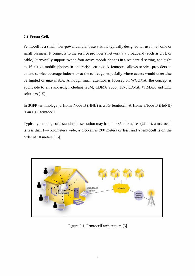
2.1.Femto Cell.

Femtocell is a small, low-power cellular base station, typically designed for use in a home or

small business. It connects to the service provider’s network via broadband (such as DSL or

cable). It typically support two to four active mobile phones in a residential setting, and eight

to 16 active mobile phones in enterprise settings. A femtocell allows service providers to

extend service coverage indoors or at the cell edge, especially where access would otherwise

be limited or unavailable. Although much attention is focused on WCDMA, the concept is

applicable to all standards, including GSM, CDMA 2000, TD-SCDMA, WiMAX and LTE

solutions [15].

In 3GPP terminology, a Home Node B (HNB) is a 3G femtocell. A Home eNode B (HeNB)

is an LTE femtocell.

Typically the range of a standard base station may be up to 35 kilometres (22 mi), a microcell

is less than two kilometers wide, a picocell is 200 meters or less, and a femtocell is on the

order of 10 meters [15].

Figure 2.1. Femtocell architecture [6]

5

2.2.BENEFITS OF FEMTO CELL.

Studies on wireless usage show that more than 50 % of all voice calls and more than 70% of

data traffic originate from indoors. Voice networks are engineered to tolerate low signal

quality, since the required data rate for voice signals is very low, on the order of 10 kb/s or

less. Data networks, on the other hand, require much higher signal quality in order to provide

the multimegabit per second data rates users have come to expect. For indoor devices,

particularly at the higher carrier frequencies likely to be deployed in many wireless

broadband systems, attenuation losses will make high signal quality and hence high data rates

very difficult to achieve. This raises the obvious question: why not encourage the end user to

install a short-range low-power link in these locations? This is the essence of the win-win of

the femtocell approach. The subscriber is happy with the higher data rates and reliability; the

operator reduces the amount of traffic on their expensive macrocell network, and can focus

its resources on truly mobile users. To summarize, the key arguments in favour of femtocells

are the following which is described in [4].

Figure 2.2 : Dense femtocellular network deployment scenario[10]

Better coverage and capacity. Due to their short transmit-receive distance,

femtocells can greatly lower transmit power, prolong handset battery life, and achieve

a higher signal-to-interference- plus-noise ratio (SINR). These translate into improved

reception — so-called five-bar coverage — and higher capacity. Because of the

reduced interference, more users can be packed into a given area in the same region of

6

spectrum, thus increasing the area spectral efficiency or, equivalently, the total

number of active users per Hertz per unit area.

Improved macrocell reliability. If the traffic originating indoors can be absorbed

into the femtocell networks over the IP backbone, the macrocell BS can redirect its

resources toward providing better reception for mobile users.

Cost benefits. Femtocell deployments will reduce the operating and capital

expenditurecosts for operators. A typical urban macrocell costs upwards of

$1000/month in site lease, and additional costs for electricity and backhaul. The

macrocell network will be stressed by the operating expenses, especially when

subscriber growth does not match the increased demand for data traffic . The

deployment of femtocells will reduce the need for adding macro-BS towers. A recent

study shows that the operating expenses scale from $60,000/year/macrocell to just

$200/year/femtocell.

Reduced subscriber turnover. Poor in-building coverage causes customer

dissatisfaction, encouraging them to either switch operators or maintain a separate

wired line whenever indoors. The enhanced home coverage provided by femtocells

will reduce motivation for home users to switch carriers.

2.3.Network Architecture.

Several FAPs are connected to a femto gateway (FGW) through a broadband ISP or another

network. The FGW acts like a concentrator and also provides security gateway functionalities

for the connected FAPs. The FGW communicates with the RNC through the CN (Core

network). The FGW manages the traffic flows for thousands of femtocells. Traffic from

different access networks comes to the FGW and is then sent to the desired destination

networks. Whenever an FAP is installed, the respective FGW provides the FAP’s position

and its authorized user list to the macrocellular BS database (DB) server through the CN [10].

It provides SON (Self organising network) mechanisms. The main functionalities of the SON

for femtocellular networks are self-configuration, self-optimization, and self-healing. Self-

configuration includes frequency allocation. Self -optimization includes transmission power

optimization, neighbour cell list optimization, coverage optimization, and mobility robustness

optimization. Self-healing includes automatic detection and solution of most of the failures.

Neighbour FAPs as well as the macrocellular BS and the neighbour FAPs coordinate with

each other. Whenever an MS desires handover in an overlaid macrocell environment, the MS

7

detects multiple neighbour FAPs because of the dense deployment of femtocells along with

the presence of macrocell coverage.

Figure 2.3 :Device to CN connectivity for femto cell deployment[10]

2.4. Other small cell networks.

1. Distributed antennas.

Operator installed spatially separated antenna elements (AEs) connected to a macro BS via a

dedicated fiber/microwave backhaul link [4].

Fig2.4. Distributed Antennas[4]

8

Benefits. a) Better coverage since user talks to nearby AE;

b) capacity gain by exploiting both macro- and micro-diversity (using multiple AEs per

macrocell user).

Shortcomings. a) Does not solve the indoor coverage problem;

b) RF interference in the same bandwidth from nearby AEs will diminish capacity;

c) backhaul deployment costs may be considerable.

2. Microcells.

Operator installed cell towers, which improve coverage in urban areas with poor

reception.

Fig 2.5. Micro cells[4]

Benefits. a) System capacity gain from smaller cell size;

b) complete operator control.

Shortcomings. a) Installation and maintenance of cell towers is prohibitively expensive;

b) does not completely solve indoor coverage problem.

9

2.5.FEMTOCELLS VS. Wi-Fi.

Key aspect Femtocells Wi-Fi

Spectrum availability

Licensed band

Must reuse operator’s

available spectrum

allocatio

Unlicensed band

Operator need not

concern with

spectrum related

issues

Indoor coverage

Up to 10-30 m.

Transmit power level

is less 1-100 mW

Up to 100 m.

Transmit power

levels of most Wi-Fi

Aps are higher up to

1W.

Interference issues

Co-channel

interference with

macrocell

Interference

avoidance and

management

techniques are

necessary.

Interference cancellation

features are there.

Network planning

Operator effort is needed for

careful frequency planning

and interference avoidance

No special effort is needed

for network planning

Data rates

WCDMA- 384

kbps,HSDPA-14.4

Mbps

LTE – 100 Mbps

WiBro (802.16) - 50

Mbps(2*2 MIMO)

WiMAX 802.16m –

up to 1 Gbps

Up to 450

Mbps(802.11n)

Up to 7

Gbps(802.11ac)

Possibility to provide

LTE like service in

3G environment

Table 2.1. Femtocells vs. Wi-Fi [15]

10

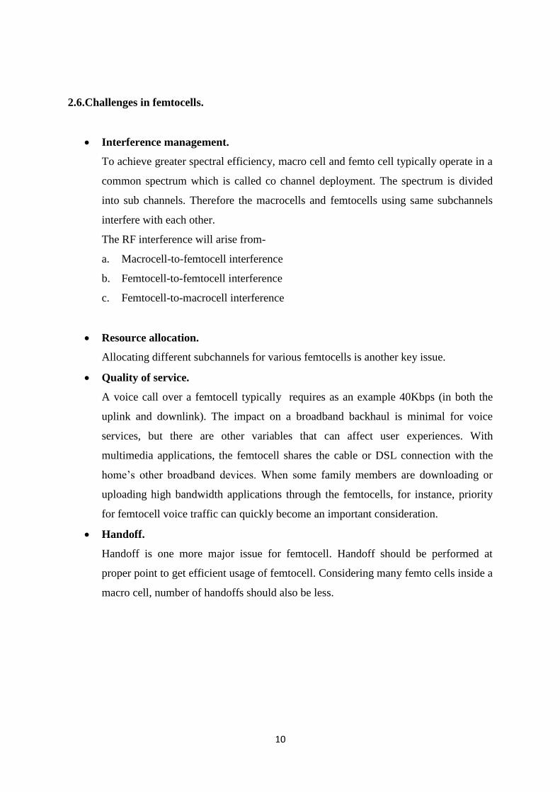
2.6.Challenges in femtocells.

Interference management.

To achieve greater spectral efficiency, macro cell and femto cell typically operate in a

common spectrum which is called co channel deployment. The spectrum is divided

into sub channels. Therefore the macrocells and femtocells using same subchannels

interfere with each other.

The RF interference will arise from-

a. Macrocell-to-femtocell interference

b. Femtocell-to-femtocell interference

c. Femtocell-to-macrocell interference

Resource allocation.

Allocating different subchannels for various femtocells is another key issue.

Quality of service.

A voice call over a femtocell typically requires as an example 40Kbps (in both the

uplink and downlink). The impact on a broadband backhaul is minimal for voice

services, but there are other variables that can affect user experiences. With

multimedia applications, the femtocell shares the cable or DSL connection with the

home’s other broadband devices. When some family members are downloading or

uploading high bandwidth applications through the femtocells, for instance, priority

for femtocell voice traffic can quickly become an important consideration.

Handoff.

Handoff is one more major issue for femtocell. Handoff should be performed at

proper point to get efficient usage of femtocell. Considering many femto cells inside a

macro cell, number of handoffs should also be less.

11

2.7.Accessing Modes in Femtocells.

Femtocells being a network used for private, enterprise or service providers purpose needs to

operate on different Accessing modes so as to provide the service for targeted user [7].

Open Access Mode:

In Open Access Mode any mobile user trying to access the femtocell service is allowed to do

so without any discrimination or extra charge similar to the macrocell. Mostly these type of

femtocells are deployed by Network Service Provider to enhance their coverage area and

QoS.

Closed Access Mode:

In Closed Access Mode the mobile user who is registered to the Femtocell is only allowed to

access the service of these Femtocell. Other users are forced to use service of macrocell even

if it is of poor service. These type of Femtocell are deployed by Organizations, Offices for

their use and good receptionof the mobile service.

Hybrid Access Mode:

It is a Combination of Open and Closed Access Modes.In this mode the preference is given to

the registered user in terms of priority and charging.

12

Chapter 3.

Handoff.

13

3.1. HANDOFF.

When a mobile user moves from coverage area of one Base Station to the coverage area of

another while engaging in active call then the transfer of call from one Base Station to the

other or from one channel to other is known as Handover.

3.2. Types of Handoff.

Handoffs are broadly classified into two categories - hard and soft handoffs. Usually, the hard

handoff can be further divided into two different types – intra and intercell handoffs. The soft

handoff can also be divided into two different types - soft handoffs and softer handoffs [3].

Hard Handoff:

A hard handoff is essentially a “break before make” connection. Under the control of the

MSC, the BS hands off the MS’s call to another cell and then drops the call. In a hard

handoff, the link to the prior BS is terminated before or as the user is transferred to the new

cell’s BS; the MS is linked to no more than one BS at any given time. Hard handoff is

primarily used in FDMA (frequency division multiple access) and TDMA (time division

multiple access), where different frequency ranges are used in adjacent channels in order to

minimize channel interference.

It is the handoff procedure primary in GSM network but also occurs in CDMA network.

Soft Handoff:

If the handoff is between two base stations but operating channel of the call remains the same

then this type of handoff is called soft handoff. In this type of Handoff, only the Mobile Base

station handling the call changes but the operating channel remains same. This type of

handover is found in CDMA network. If the sectors are from the same physical cell site(a

sectored site), it is referred to as softer handoff.

14

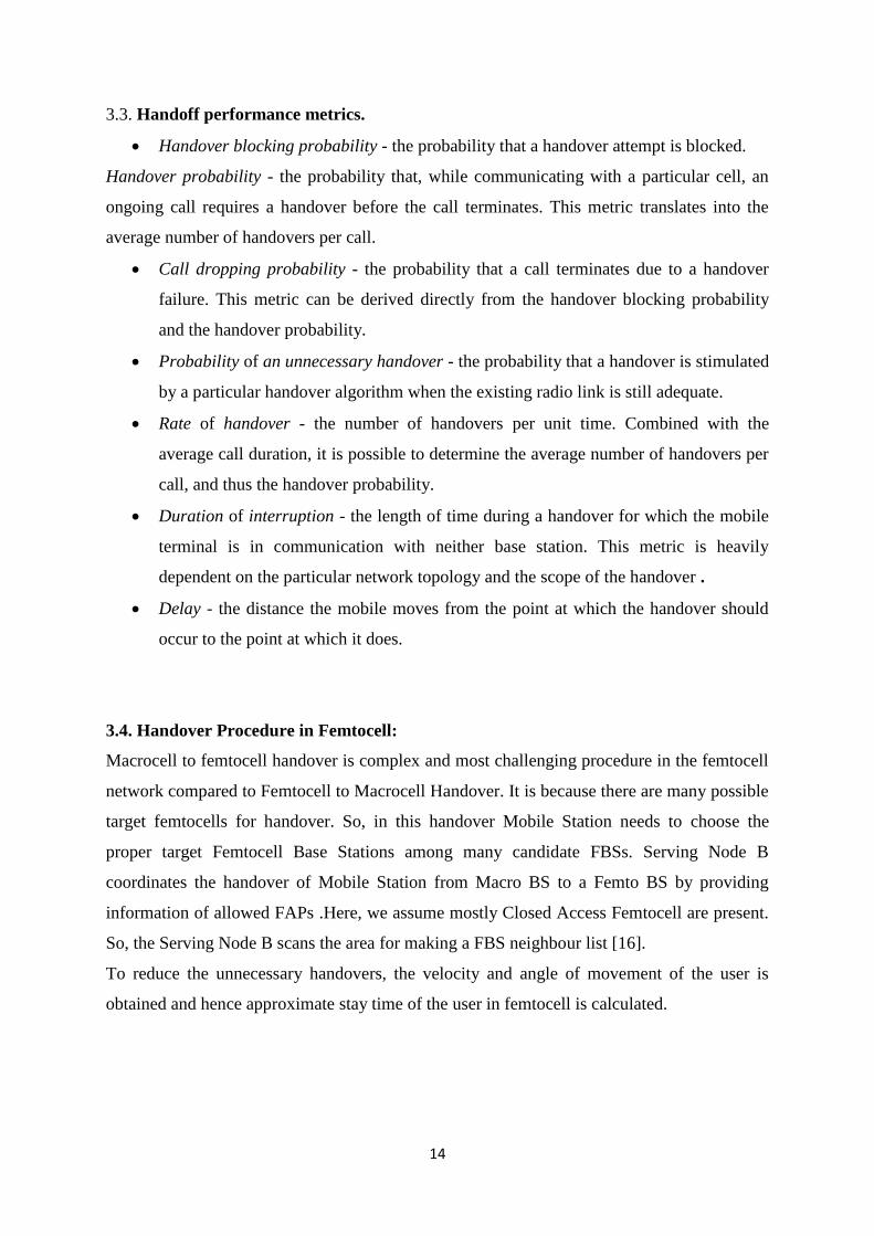
3.3. Handoff performance metrics.

Handover blocking probability - the probability that a handover attempt is blocked.

Handover probability - the probability that, while communicating with a particular cell, an

ongoing call requires a handover before the call terminates. This metric translates into the

average number of handovers per call.

Call dropping probability - the probability that a call terminates due to a handover

failure. This metric can be derived directly from the handover blocking probability

and the handover probability.

Probability of an unnecessary handover - the probability that a handover is stimulated

by a particular handover algorithm when the existing radio link is still adequate.

Rate of handover - the number of handovers per unit time. Combined with the

average call duration, it is possible to determine the average number of handovers per

call, and thus the handover probability.

Duration of interruption - the length of time during a handover for which the mobile

terminal is in communication with neither base station. This metric is heavily

dependent on the particular network topology and the scope of the handover .

Delay - the distance the mobile moves from the point at which the handover should

occur to the point at which it does.

3.4. Handover Procedure in Femtocell:

Macrocell to femtocell handover is complex and most challenging procedure in the femtocell

network compared to Femtocell to Macrocell Handover. It is because there are many possible

target femtocells for handover. So, in this handover Mobile Station needs to choose the

proper target Femtocell Base Stations among many candidate FBSs. Serving Node B

coordinates the handover of Mobile Station from Macro BS to a Femto BS by providing

information of allowed FAPs .Here, we assume mostly Closed Access Femtocell are present.

So, the Serving Node B scans the area for making a FBS neighbour list [16].

To reduce the unnecessary handovers, the velocity and angle of movement of the user is

obtained and hence approximate stay time of the user in femtocell is calculated.

15

RSS BASED HADNOFF CRITERION.

The primary criterion for handoff between a macrocell to femtocell is as follows

sm < sm,th and sf > sm + Δ (3.1)

where sm,th and Δ represent the minimum RSS level from a serving macro BS and the value of

hysteresis, respectively. And sm and sf are the received signal powers from macro and femto

base station respectively which can be calculated by the following equations

sm = Pm,tx − PLm − um (3.2)

sf = Pf,tx − PLf − uf (3.3)

Transmit power from macro cell and femto cell are Pm,tx & Pf,tx and path losses are PLm[k] and

PLf [k] from the macro BS and the femto BS. Um[k] and uf [k] represent the log-normal

shadowing with mean zero and variance σ2

m and σ2 f , respectively [1].

3.5. Temporary Femtocell visitor.

We define temporary femtocell visitor using mathematical notations and present a new

handover decision criterion to prevent unnecessary handover. Firstly, we use the threshold

time Tth to identify temporary femtocell visitor. Tth can be set differently depending on the

administration policy of each femtocell. If handovered user stays in the femtocell for more

than Tth, we assume that it is appropriate femtocell user (appropriate handover). Conversely,

if handovered user stays in the femtocell less than Tth, it becomes temporary femtocell visitor

(unnecessary handover). Thus, we define a new criterion of macro → femto handover as

follows:

Sf > Sth and Tc > Tth (3.4)

where Sf denotes the received signal strength of femtocell, Sth denotes the predefined

threshold value, Tc is cell residence time of user. Our scheme is to predict Tc using future

mobility prediction scheme so that we can perform selective macro → femto handover not to

accept temporary femtocell visitor [14].

16

3.6. TTT.

UE speed is a very important factor in handoff. It should stay inside the femtocell at least for

certain amount of time. Because basically the use of femtocell is not for high speed mobile

users. This minimum amount of time UE needs to stay for handoff is called time to

trigger(TTT). Therefore now condition for handoff is

Sf > Sm + Δ for TTT (3.5)

And for femtocell to femtocell handoff

Sf1 > Sf2 + Δ for TTT (3.6)

If we know the speed of the user, we can estimate the time it will reside in the femtocell.

Then it would be easy to make decision for handoff[ 16].

3.7. SINR criterion.

Now for more accuracy, we will also take into account SINR value at user from both cellular

network. The condition added for macrocell to femtocell handoff is as follows

SINRf > SINRm (3.7)

Calculation of SINR.

Interference and noise are present for both macrocell and femtocell. The value of SINR for

macrocell and femtocell are

SINRm =

(3.8)

SINRf =

(3.9)

RSP is received signal power m0 and f0 are current macrocell and femtocell. N is noise

power.

N = N0B

N0 = -174 dBm/Hz and bandwidth = 10 MHz

N = -174 + 10log (107)

= -104 dBm

17

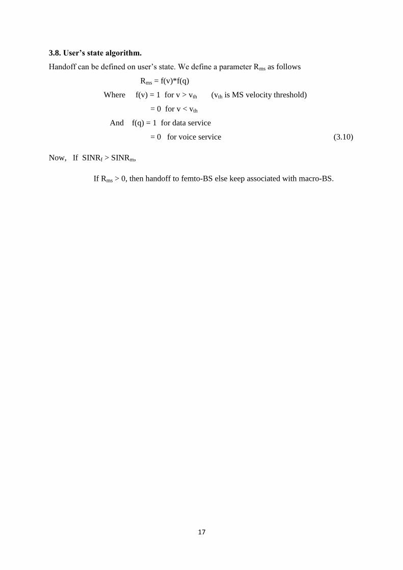
3.8. User’s state algorithm.

Handoff can be defined on user’s state. We define a parameter Rms as follows

Rms = f(v)*f(q)

Where f(v) = 1 for v > vth (vth is MS velocity threshold)

= 0 for v < vth

And f(q) = 1 for data service

= 0 for voice service (3.10)

Now, If SINRf > SINRm,

If Rms > 0, then handoff to femto-BS else keep associated with macro-BS.

18

Chapter 4.

Femto cell performance

evaluation.

19

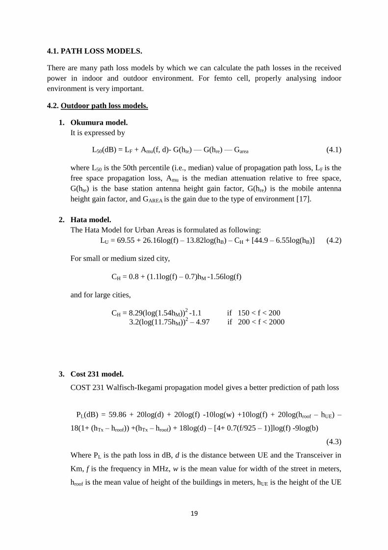
4.1. PATH LOSS MODELS.

There are many path loss models by which we can calculate the path losses in the received

power in indoor and outdoor environment. For femto cell, properly analysing indoor

environment is very important.

4.2. Outdoor path loss models.

1. Okumura model.

It is expressed by

L50(dB) = LF + Amu(f, d)- G(hte) — G(hre) — Garea (4.1)

where L50 is the 50th percentile (i.e., median) value of propagation path loss, LF is the

free space propagation loss, Amu is the median attenuation relative to free space,

G(hte) is the base station antenna height gain factor, G(hre) is the mobile antenna

height gain factor, and GAREA is the gain due to the type of environment [17].

2. Hata model.

The Hata Model for Urban Areas is formulated as following:

LU = 69.55 + 26.16log(f) – 13.82log(hB) – CH + [44.9 – 6.55log(hB)] (4.2)

For small or medium sized city,

CH = 0.8 + (1.1log(f) – 0.7)hM -1.56log(f)

and for large cities,

CH = 8.29(log(1.54hM))2

-1.1 if 150 < f < 200

3.2(log(11.75hM))2 – 4.97 if 200 < f < 2000

3. Cost 231 model.

COST 231 Walfisch-Ikegami propagation model gives a better prediction of path loss

PL(dB) = 59.86 + 20log(d) + 20log(f) -10log(w) +10log(f) + 20log(hroof – hUE) –

18(1+ (hTx – hroof)) +(hTx – hroof) + 18log(d) – [4+ 0.7(f/925 – 1)]log(f) -9log(b)

(4.3)

Where PL is the path loss in dB, d is the distance between UE and the Transceiver in

Km, f is the frequency in MHz, w is the mean value for width of the street in meters,

hroof is the mean value of height of the buildings in meters, hUE is the height of the UE

20

in meters, hTx is the height of the transceiver in meters, b is the mean value of building

separation in meters.

4. UMi Model.

This model is designed specifically for small cells with high user densities and traffic

loads in city centres and dense urban areas. The path loss for the LoS condition is

calculated as

22 log10 d + 42 + 20 log10(fc/5) 10m<d<dBP

LUMi,LOS = 40 log10 d + 9.2 – 18log10 heNB

-18log10 hUE + 2 log10(fc/5) dBP<d<5km (4.4)

Here, the distance between transmitter and receiver is d, the effective breakpoint distance is

calculated as dBP = 4heNBhUEfc/c, where fc is the centre frequency in Hz and h′eNB and h′UE are

the effective antenna heights for the eNB and UE, respectively [12].

The path loss for the non-line-of-sight (nLoS) model is computed as

LUMi,NLOS = 36.7 log10 d + 40.9 + 26 log10(fc/5) 10m<d<5km (4.5)

But in simulation for macrocell/femtocell handoff phenomenon, rather than using these

models, a simplified model is used. It is given below

Path loss L(dB) = 128.1 + 37.6 log(d) (4.6)

Where d is the distance between transmitter and receiver.

4.3.Indoor path loss models.

1. Indoor hotspot model.

This model is used to model the channel for links lying inside the femto-cells. The

LoS path loss is calculated as

LInH, LoS = 16.9 log10(d) + 46.8 + 20 log10(fc/5); 3m < d <100m. (4.7)

The path loss for the nLoS model is calculated as

LInH, nLoS = 43.3 log10(d) + 25.5 + 20 log10(fc/5); 10m < d <150m. (4.8)

2. ITU indoor propagation model.

For indoor path loss ITU indoor path loss model is taken which is as follows [17]

21

PL(dB) = 20 log(f) + N log(d) + Pf(n) -28 (4.9)

where,

L = the total path loss (dB).

f = frequency of transmission.(MHz).

d = Distance. Unit: metre (m).

N = The distance power loss coefficient.

n = Number of floors between the transmitter and receiver.

Pf(n) = the floor loss penetration factor.

For residential area N= 28 and Pf(n) = 4n

4.4.Outdoor to indoor (and vice-versa) model.

The UMi path loss model assists in modelling the indoor↔outdoor path loss as

Loi = Lb + Ltw + Lin; 50m < d < 5 km. (4.10)

Here, Lb is the basic path loss calculated using the UMi model as Lb = LUMi(dout +din). The

parameters dout and din refer to the outdoor and indoor distances respectively. The parameter

Ltw, is the wall penetration loss and Lin, dependent on the indoor distance alone, is calculated

as Lin = 0.5din [12].

4.5.Capacity calculation in femto cells.

Here an LTE OFDMA-FDD system is considered with system bandwidth W which is divided

into NRB resource blocks(RBs), each of bandwidth WRB such that

W=NRBWRB (4.11)

Where the RB represents the basic OFDMA time frequency unit. Two RBs comprise one

subframe and ten subframes together make one LTE frame.

Universal frequency reuse is considered, so that both macro and femto-cells utilise the entire

system bandwidth W, in the uplink (UL) and DL.

The received UL or DL signal power associated with UE u on RB n, Yu

n is given by

Yu

n = Pu

n Σ Gu

m, vu

n + Inu

+ ηRB (4.12)

Where Gu

m, vu

n is the channel gain between UE u and its serving HeNB or eNB vu, observed

at receive antenna m and at RB n. Furthermore, ηRB accounts for thermal noise per RB which

22

is constant across all RBs and both directions of communication. In the DL, the transmit

power is set to Pu

n= PeNB and Pu

n = PHeNB if UE u is served by an eNB or HeNB, respectively.

In the UL, Pu

n = PFUE or Pun = PMUE, depending on whether the UE in question is served by a

HeNB or an eNB, respectively. The values PHeNB, PeNB, PMUE and PFUE are constant across all

RBs. The aggregate interference Iu

n is composed of macro and femto-cell interference [12].

Inu = Σ G

um,

in Pm + Σ G

um,

in Pf (4.13)

iϵMint iϵFint

where the first and second addends represent the macro and femto-cell interference,

respectively. Here, Pm is set respectively to PeNB and PMUE in the DL and UL. Similarly, Pf is

set respectively to PHeNB and PFUE in the DL and UL. Mint represents the set of interfering

macro UEs in the UL and the set of interfering eNBs in the DL. Similarly, Fint denotes the set

of interfering femto Ues in the UL and the set of interfering HeNBs in the DL.

The SINR observed in the UL or DL with regards to UE u on RB n,

Γnu = Pn

u Σ Gm

u,n

vu (4.14)

Inu

+ ηRB

Thus the capacity Cu is calculated by shannon’s law

Cu = Σ WRB. log2(1+ γnu) (4.15)

4.6.Channel model.

The channel gain, Gu

n,vm between a transmitter v and a receiver u, observed at receive

antenna m on RB n is composed of distance dependent path loss, log-normal shadowing and

channel variations due to frequency-selective fading

Gu

n,vm = |H

un,

vm |

2 . 10

(-L+Xσ

)/10 (4.16)

where H u

n,vm denotes the channel transfer function (CTF) between transmitter v and receiver

u, observed at receive antenna m and on RB n, L is the distance-dependent path loss (in dB),

and Xσ is the log-normal shadowing value (in dB) with standard deviation σ [12].

23

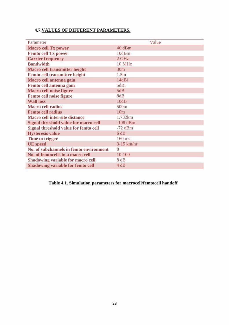
4.7.VALUES OF DIFFERENT PARAMETERS.

Parameter Value

Macro cell Tx power 46 dBm

Femto cell Tx power 10dBm

Carrier frequency 2 GHz

Bandwidth 10 MHz

Macro cell transmitter height 30m

Femto cell transmitter height 1.5m

Macro cell antenna gain 14dBi

Femto cell antenna gain 5dBi

Macro cell noise figure 5dB

Femto cell noise figure 8dB

Wall loss 10dB

Macro cell radius 500m

Femto cell radius 10m

Macro cell inter site distance 1.732km

Signal threshold value for macro cell -108 dBm

Signal threshold value for femto cell -72 dBm

Hysteresis value 6 dB

Time to trigger 160 ms

UE speed 3-15 km/hr

No. of subchannels in femto environment 8

No. of femtocells in a macro cell 10-100

Shadowing variable for macro cell 8 dB

Shadowing variable for femto cell 4 dB

Table 4.1. Simulation parameters for macrocell/femtocell handoff

24

4.8.Simulation results.

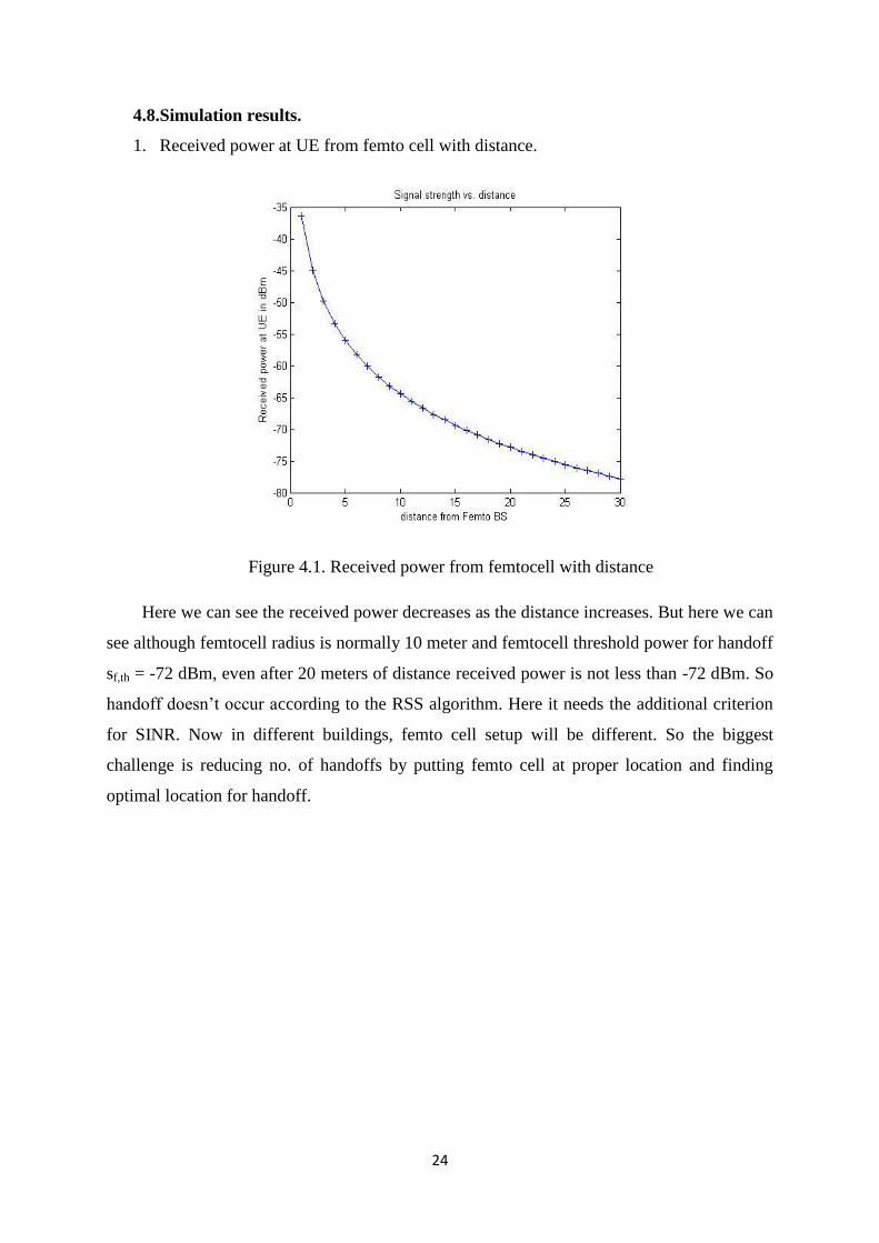
1. Received power at UE from femto cell with distance.

Figure 4.1. Received power from femtocell with distance

Here we can see the received power decreases as the distance increases. But here we can

see although femtocell radius is normally 10 meter and femtocell threshold power for handoff

sf,th = -72 dBm, even after 20 meters of distance received power is not less than -72 dBm. So

handoff doesn’t occur according to the RSS algorithm. Here it needs the additional criterion

for SINR. Now in different buildings, femto cell setup will be different. So the biggest

challenge is reducing no. of handoffs by putting femto cell at proper location and finding

optimal location for handoff.

25

2. Received power at MS(dBm) vs distance(meter) from macro cell in cost 231 model

and simplified outdoor path loss model.

Figure 4.2. Received power from macrocell with distance

This graph depicts the received power at MS from macro base station with distance. Two

curves are according to two different path loss models. We can have an idea of handoff

performance between macro cell and femto cell if we compare this graph and the previous

one. Exactly at which point handoff is taking place. It also depends on how the macro cell

and femto cells are distributed.

26

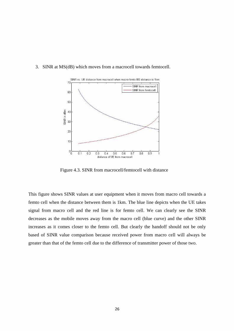
3. SINR at MS(dB) which moves from a macrocell towards femtocell.

Figure 4.3. SINR from macrocell/femtocell with distance

This figure shows SINR values at user equipment when it moves from macro cell towards a

femto cell when the distance between them is 1km. The blue line depicts when the UE takes

signal from macro cell and the red line is for femto cell. We can clearly see the SINR

decreases as the mobile moves away from the macro cell (blue curve) and the other SINR

increases as it comes closer to the femto cell. But clearly the handoff should not be only

based of SINR value comparison because received power from macro cell will always be

greater than that of the femto cell due to the difference of transmitter power of those two.

27

4. Throughput.

Figure 4.4. Throughput from macrocell/femtocell with distance

In this figure, we can see the throughput variation as the user moves from femto cell towards

macro cell. It can also be noted that throughput is much higher near femtocell because of its

high bandwidth and so it’s high coverage in indoors.

4.9.Femtocell interference.

Till now we considered macro/femto network with only one macro cell and one femto cell.

Here we will be considering no. of femtocells to show how it affects handoff.

When FMCs and UEs transmit their signals in the same frequency band (same subchannel)

within the same environment, interference will occur.

28

Downlink OFDMA.

FMCs transmits in different subcarriers than BS in OFDMA systems, which help in

interference avoidance. In addition, in OFDMA system, FMCs are deployed in subchannels

distribution. In downlink the UE which is indoors and receiving signal from indoor FMC

must have different subchannels from the UE which is outdoors and receiving signal directly

from the outdoors BS [9].

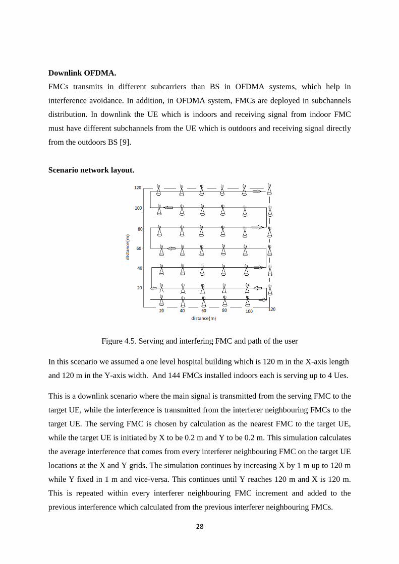
Scenario network layout.

Figure 4.5. Serving and interfering FMC and path of the user

In this scenario we assumed a one level hospital building which is 120 m in the X-axis length

and 120 m in the Y-axis width. And 144 FMCs installed indoors each is serving up to 4 Ues.

This is a downlink scenario where the main signal is transmitted from the serving FMC to the

target UE, while the interference is transmitted from the interferer neighbouring FMCs to the

target UE. The serving FMC is chosen by calculation as the nearest FMC to the target UE,

while the target UE is initiated by X to be 0.2 m and Y to be 0.2 m. This simulation calculates

the average interference that comes from every interferer neighbouring FMC on the target UE

locations at the X and Y grids. The simulation continues by increasing X by 1 m up to 120 m

while Y fixed in 1 m and vice-versa. This continues until Y reaches 120 m and X is 120 m.

This is repeated within every interferer neighbouring FMC increment and added to the

previous interference which calculated from the previous interferer neighbouring FMCs.

29

Propagation loss model.

In indoor residential premises, the path loss model we took as before

PL(dB) = 20 log(f) + 28 log(d) – 24 (4.17)

= 42 + 28 log10(d) where, f=2000 MHz

This equation is used to evaluate path loss power between serving FAP and target UE as well

as interferer FMCs and target UE where d is the distance between them and obtained by

d =[ (UE(x) – X(k))2 + (UE(y) – Y(k))

2]

0.5 (4.18)

Here UE(x) and UE(y) are the x and y coordinates of target UE and X(k) and Y(k) are the x

and y coordinates of serving femto cell and kth

interfering femtocells in respective cases [9].

FAP-UE interference analysis.

Interference occurs in downlink when the signal transmitted from the specific FMC to the

target UE overlap in subchannel with the signals which transmits from the neighbouring

FMCs. This simulation neglect WiMAX BS to FMC interference, and concentrate on the

FMC, neighbouring FMCs and UE interference.

Si = Pi · Gi · Li · PLix · Gx · LxdB (4.19)

where Si is the received signal by the target UE from the serving FMC, Pi is the serving FMC

transmission power, Gi is the serving FMC antenna gain, Li is the serving FMC cable loss,

PLix is the path loss between the serving FMC and the target UE, Gx is the target UE antenna

gain, Lx is the target UE loss.

Sj = Pj · Gj · Lj · PLjx · Gx · LxdB (4.20)

hereSj is the received signals from the interferer FMC by the target UE, Gj is the interferer

neighbouring FMC antenna gain, Lj is the interferer neighbouring FMC cable loss, PLjx is the

path loss between the interferer neighbouring FMC and the target UE. Our simulation will

accumulate to compute the interference value that caused by all interferers neighbouring

FMCs on the target UE. The transmitted signal from the specific FMC to the target UE is

considered as the mean signal, and the sum of the transmitted signals of all interferers

neighbouring FMCs to the target UE as the interference [9].

30

SINR = Si / ( Σ Sj + σ) dB (4.21)

Where, Si is the transmitted signal from the serving FMC to the target UE, Sj is the

accumulation of all the transmitted signals from the interferer FMCs to the target UE.

Σ = n + nF dB

n = - 174 – 30 + 10 log10 (f) dB (4.22)

here, n is the thermal noise in dB, f is the Channel bandwidth frequency which is 5 MHz and

nF is the noise Figure of the target UE which is 8 dB. σ is the sum of the thermal noise and

the target UE noise Figure.

Simulation results.

The desired FMC coverage distance is suggested to be 10 m in each direction and 10 m by 10

m area will be covered by the individual FMC, here for the whole area we used 144 FMCs.

The interference of the target UE is evaluated in the grids of the X and Y axis’s by

substituting the target UE location and calculates the average interference. The simulation

evaluates the interference, SINR, and the probability of connection.

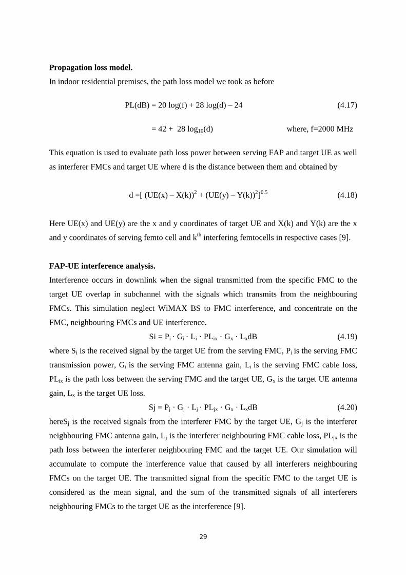
1. Interference.

Figure 4.6. Interference with no. of femtocells

31

Result clearly shows that as number of femtocells increases, magnitude of interference to the

target femtocell increases gradually. The reason being the number of interfering femtocells is

increasing.

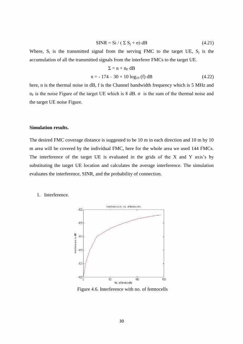
2. SINR.

Figure 4.7. SINR with no. of femtocells

This figure depicts the signal-to-interference and noise ratio SINR, which is calculated by the

main signal that transmitted from the served FMC to the target UE, and the interference that

are accumulated from all the neighbouring FMCs to the target UE. The SINR increases

slightly with the increase of FMCs number.

32

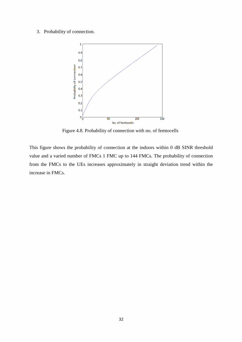
3. Probability of connection.

Figure 4.8. Probability of connection with no. of femtocells

This figure shows the probability of connection at the indoors within 0 dB SINR threshold

value and a varied number of FMCs 1 FMC up to 144 FMCs. The probability of connection

from the FMCs to the UEs increases approximately in straight deviation trend within the

increase in FMCs.

33

Chapter 5.

Handoff probabilities

and failures.

34

5.1. Handoff probabilities and call arrival rates in macro/femto hierarchical

environment.

Three important handoff probabilities for normal cellular network to femto network handoff

are

Pf|m,RSS = P{sm > sm,th , sf > sm + Δ | M}

Pf|m,SINR = P{SINRf > SINRm | M}

Pf|m,SINR & user = P{SINRf > SINRm , Rms > 0 | M} (5.1)

M is the event that the user is currently connected to macro cell.

λo,f and λo,m denote the total originating call arrival rates considering all n number of

femtocells within a macrocell coverage area and only the macrocell coverage area,

respectively. λh,mm, λh,ff, λh,fm, and λh,mf denote the total macrocell-to-macrocell, femtocellto-

femtocell, femtocell-to-macrocell, and macrocell-tofemtocell handover call arrival rates

within the macrocell coverage area, respectively. PB,m (PB,f ) is the new originating call

blocking probability in the macrocell (femtocell) system. PD,m (PD,f ) is the handover call

dropping probability in the macrocell (femtocell) system [10].

We also use two threshold levels of SNIR to admit a call in the system. The first threshold

level Γ1 is the minimum level of the received SNIR that is needed to connect a call to any

FAP. The second signal level Γ2 is higher than Γ1. The second threshold is used in the CAC to

reduce the unnecessary macrocell-to-femtocell handovers. We assume that for a femtocell-to-

femtocell handover, the probability that the received SINR of the T-FAP is greater Γ2 and is

represented by α, and the received SINR of the T-FAP is between Γ1 and Γ2 and is

represented by β.

Equating the net rate of calls entering a cell and requiring handover to those leaving the cell,

the handover call arrival rates are calculated as follows

35

The macrocell-to-macrocell handover call arrival rate is

λh,mm = Ph,mm . (1-PB,m)(λm,o + λf,oPB,f) + (1-PD,m){ λh,fm + λh,ff(1-α+αPD,f)

1 – Ph,mm(1-PD,m) (5.2)

the macrocell-to-femtocell handover call arrival rate is

λh,mf = Ph,mf . (1-PB,m)(λm,o + λf,oPB,f) + (1-PD,m){ λh,fm + λh,ff(1-α+αPD,f)

1 – Ph,mm(1-PD,m) (5.3)

the femtocell-to-femtocell handover call arrival rate is

λh,ff = Ph,ff . λf,o (1-PB,f) + λh,mf(1-PD,f)

1-Ph,ff(1-PD,f){α+(1- α)PD,m} (5.4)

and the femtocell-to-macrocell handover call arrival rate is

λh,fm = Ph,fm . λf,o (1-PB,f) + λh,mf(1-PD,f)

1-Ph,ff(1-PD,f){α+(1- α)PD,m} (5.5)

where Ph,mm, Ph,mf, Ph,ff, and Ph,fm are the macrocell-tomacrocell handover probability,

macrocell-to-femtocell handover probability, femtocell-to-femtocell handover probability,

and femtocell-to-macrocell handover probability, respectively.

The probability of handover depends on several factors such as the average call duration, cell

size, and average user velocity. The handover probabilities from a femtocell and to a

femtocell in integrated femtocell/macrocell networks also depend on the density of femtocells

and the average size of femtocell coverage areas. We derive the formulas for Ph,mm, Ph,mf, Ph,ff,

and Ph,fm as follows which is described in [10].

Macrocell to macrocell handoff probability

Ph,mm = ηm/(ηm+μ) (5.6)

Femtocell to macrocell handoff probability

Ph,fm = [1-n(rf/rm)2]. ηf/(ηf+μ) (5.7)

Femtocell to femtocell handoff probability

Ph,ff = (n-1)( rf/rm)2. ηf/(ηf+μ) (5.8)

36

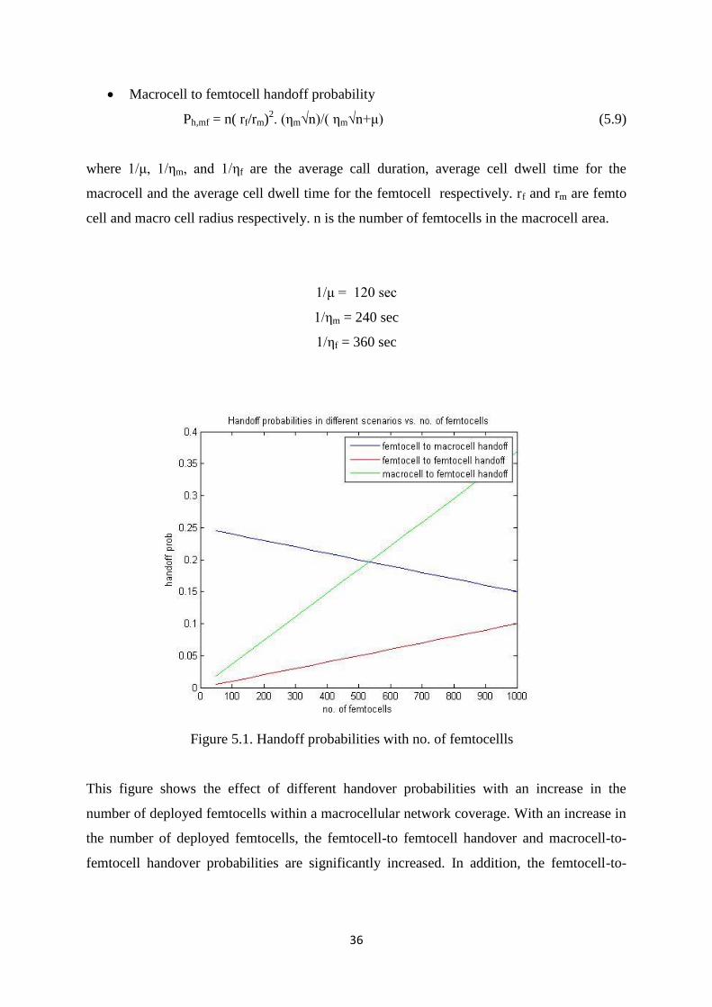
Macrocell to femtocell handoff probability

Ph,mf = n( rf/rm)2. (ηm√n)/( ηm√n+μ) (5.9)

where 1/μ, 1/ηm, and 1/ηf are the average call duration, average cell dwell time for the

macrocell and the average cell dwell time for the femtocell respectively. rf and rm are femto

cell and macro cell radius respectively. n is the number of femtocells in the macrocell area.

1/μ = 120 sec

1/ηm = 240 sec

1/ηf = 360 sec

Figure 5.1. Handoff probabilities with no. of femtocellls

This figure shows the effect of different handover probabilities with an increase in the

number of deployed femtocells within a macrocellular network coverage. With an increase in

the number of deployed femtocells, the femtocell-to femtocell handover and macrocell-to-

femtocell handover probabilities are significantly increased. In addition, the femtocell-to-

37

macrocell handover probability is very high. Thus, the management of this large number of

handover calls is the important issue for dense femtocellular network deployment.

5.2. Handover failures.

Inbound mobility and outbound mobility are supported in LTE-based femtocell system .

Inbound mobility corresponds to the handoff (HO) from the macro cell to the femtocell,

outbound mobility to the macro cell from the femtocell. For inbound mobility, the UE

connecting to the macro cell can move inside the femtocell without the occurrence of radio

link failure (RLF) since the macro and femtocells use different frequency bands. However,

the failure during outbound HO will lead to the disconnection of UE from the femtocell,

which causes serious degradation of user’s experience [11].

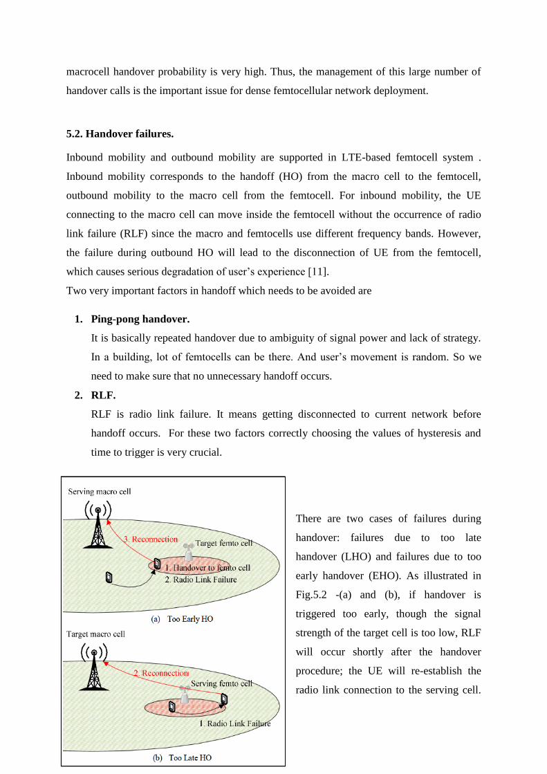
Two very important factors in handoff which needs to be avoided are

1. Ping-pong handover.

It is basically repeated handover due to ambiguity of signal power and lack of strategy.

In a building, lot of femtocells can be there. And user’s movement is random. So we

need to make sure that no unnecessary handoff occurs.

2. RLF.

RLF is radio link failure. It means getting disconnected to current network before

handoff occurs. For these two factors correctly choosing the values of hysteresis and

time to trigger is very crucial.

There are two cases of failures during

handover: failures due to too late

handover (LHO) and failures due to too

early handover (EHO). As illustrated in

Fig.5.2 -(a) and (b), if handover is

triggered too early, though the signal

strength of the target cell is too low, RLF

will occur shortly after the handover

procedure; the UE will re-establish the

radio link connection to the serving cell.

38

On the other hand, if handover is triggered too late, though the signal strength of the serving

cell is already too low, RLF will occur before the handover is initiated or during the handover

procedure; the UE will re-establish the radio link connection to the target cell.

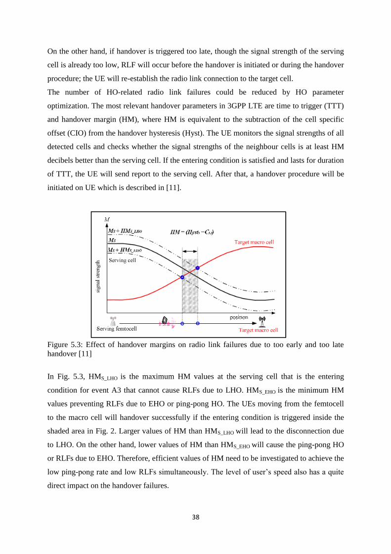
The number of HO-related radio link failures could be reduced by HO parameter

optimization. The most relevant handover parameters in 3GPP LTE are time to trigger (TTT)

and handover margin (HM), where HM is equivalent to the subtraction of the cell specific

offset (CIO) from the handover hysteresis (Hyst). The UE monitors the signal strengths of all

detected cells and checks whether the signal strengths of the neighbour cells is at least HM

decibels better than the serving cell. If the entering condition is satisfied and lasts for duration

of TTT, the UE will send report to the serving cell. After that, a handover procedure will be

initiated on UE which is described in [11].

Figure 5.3: Effect of handover margins on radio link failures due to too early and too late

handover [11]

In Fig. 5.3, HMS_LHO is the maximum HM values at the serving cell that is the entering

condition for event A3 that cannot cause RLFs due to LHO. HMS_EHO is the minimum HM

values preventing RLFs due to EHO or ping-pong HO. The UEs moving from the femtocell

to the macro cell will handover successfully if the entering condition is triggered inside the

shaded area in Fig. 2. Larger values of HM than HMS_LHO will lead to the disconnection due

to LHO. On the other hand, lower values of HM than HMS_EHO will cause the ping-pong HO

or RLFs due to EHO. Therefore, efficient values of HM need to be investigated to achieve the

low ping-pong rate and low RLFs simultaneously. The level of user’s speed also has a quite

direct impact on the handover failures.

39

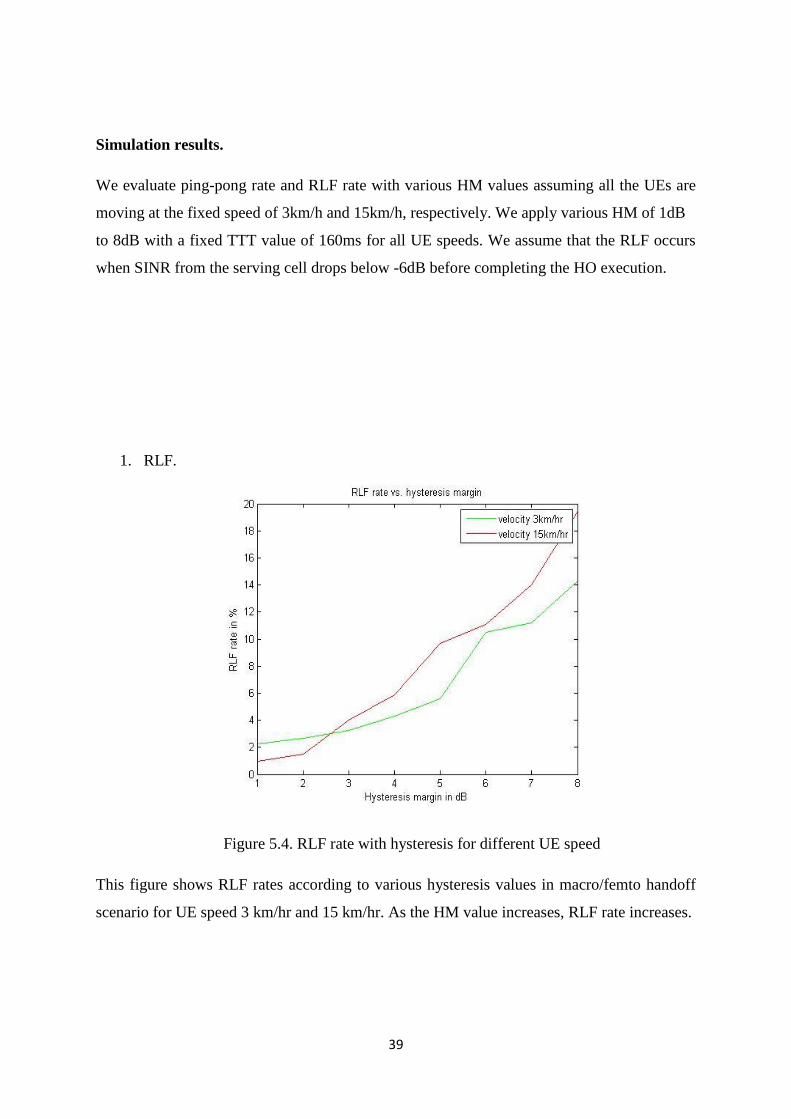
Simulation results.

We evaluate ping-pong rate and RLF rate with various HM values assuming all the UEs are

moving at the fixed speed of 3km/h and 15km/h, respectively. We apply various HM of 1dB

to 8dB with a fixed TTT value of 160ms for all UE speeds. We assume that the RLF occurs

when SINR from the serving cell drops below -6dB before completing the HO execution.

1. RLF.

Figure 5.4. RLF rate with hysteresis for different UE speed

This figure shows RLF rates according to various hysteresis values in macro/femto handoff

scenario for UE speed 3 km/hr and 15 km/hr. As the HM value increases, RLF rate increases.

40

2. Ping-Pong.

Figure 5.5. Ping-Pong rate with hysteresis for different UE speed

Here we can see as the HM value increases, the ping-pong rate decreases. Therefore, the

criteria for selecting proper HM values is to minimize pingpong rates while keeping RLF rate

below 2%, which will lead to the best trade-off between RLF rate and ping-pong rate.

From this evaluation we chose the value for hysteresis as 6 dB when the user velocity is

3km/hr which we will be using for later simulations.

41

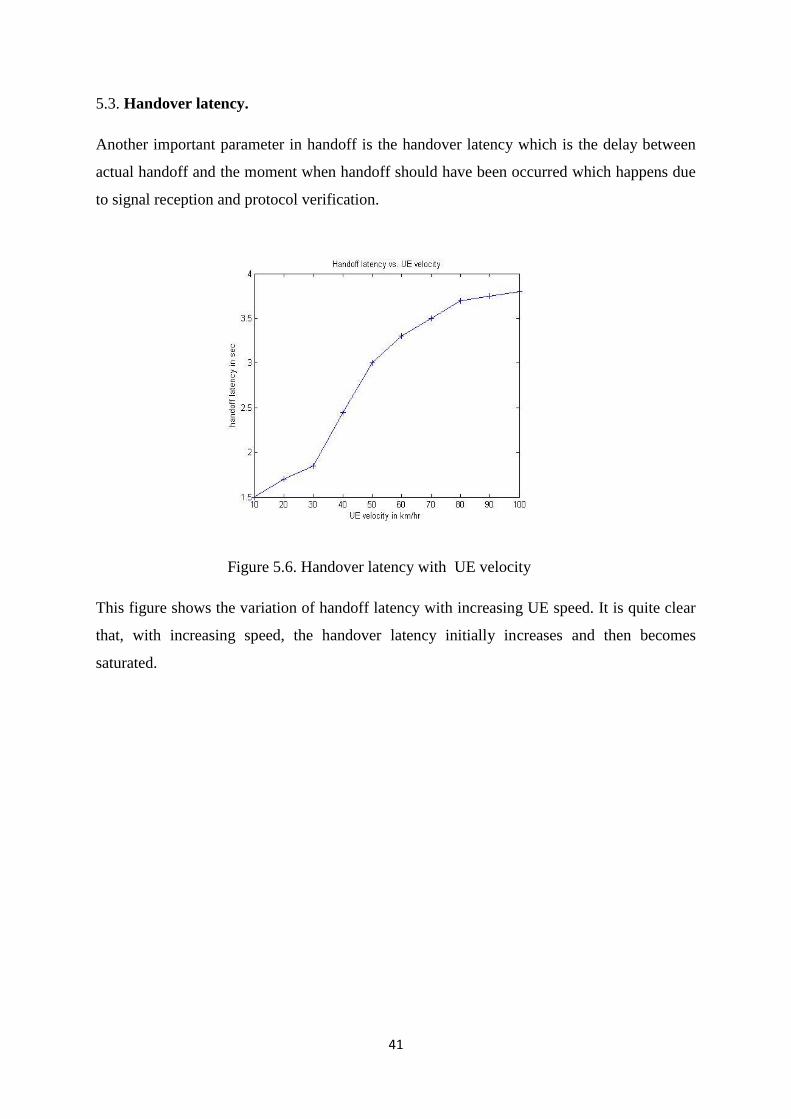
5.3. Handover latency.

Another important parameter in handoff is the handover latency which is the delay between

actual handoff and the moment when handoff should have been occurred which happens due

to signal reception and protocol verification.

Figure 5.6. Handover latency with UE velocity

This figure shows the variation of handoff latency with increasing UE speed. It is quite clear

that, with increasing speed, the handover latency initially increases and then becomes

saturated.

42

Chapter 6.

Proposed algorithm.

43

Proposed algorithm.

The main objective of handoff algorithm is to decide an optimal connection with

respect to user or system performance, while minimizing handoff latency and the number of

handoffs. The most commonly used algorithm is based on the comparison of RSS’s and the

concept of hysteresis and threshold. The threshold sets a minimum RSS from a serving BS

and the hysteresis adds a margin to the RSS from the serving BS over that from a target BS.

This handoff decision algorithm especially can be utilized by a mobile station (MS) moving

from a macrocell to a femtocell. Here, it is assumed that the MS has a capability to detect

neighbouring femtocells. In hierarchical macro/femtocell networks, there are two interesting

requirements about mobility management. First, an MS gives higher priority to a femto BS

over a macro BS when the MS selects its serving BS. A reason for this requirement is not

only the high utilization of femtocells but also the usage of different billing models between

two types of cells. Thus, performing handoff from a macrocell to a femtocell efficiently can

be seen as a way of increasing user satisfaction. Second, the deployment of femtocells should

not cause drastic changes on mobility management procedures used in conventional

macrocell networks. It means that conventional methods, such as cell scanning and handoff,

can also be applied to the hierarchical macro/femto-cell networks. In the aspect of fulfilling

these requirements, various handoff algorithms based on received signal strength (RSS) with

hysteresis and threshold have a common and critical drawback: that is, a criterion for handoff

from a macrocell to a femtocell is hard to be satisfied when the femto BS is installed in the

center or inner region of the macrocell. This phenomenon is caused by much lower transmit

power of the femto BS compared to that of the macro BS. The typical values of the transmit

power are 10 dBm for the femto BS and 46 dBm for the macro BS, respectively. Therefore, it

is necessary to design a suitable handoff decision algorithm for the situation where a user’s

call is handed off from a macrocell to a femtocell.

44

Fig 6.1 : Handoff scenario of MS moving from macrocell to femtocell [1]

The main idea of a proposed RSS based handoff decision algorithm is to multiply the values

of RSS by some constant from a target femto base station which is currently connected to

macro cell in the consideration of each femto BS’s own situation for efficient handoff which

was not occurring due to the huge transmit power difference between macro cell and femto

cell.

Sfmod = αSf where α>1 (6.1)

Figure 6.2. Mobile user at macrocell/femtocell boundary scenario

45

6.1.Mathematics of the algorithm.

Let the distance between macro cell and femto cell be D km. Femto cell radius is rf which is

taken as 10m.

Macro cell transmit power = 46 dBm

Femto cell transmit power = 10 dBm

Macrocell path loss = 128 + 37.6 log10d(km)

Femtocell path loss(simplified) = 42 + 28log10d(m)

Therefore at femtocell boundary, received signal strength from femtocell should not be less

than that of macro cell.

Sf =[10-(42+28log10d(m))]

Sm= 46- [128+37.6 log10(D-d)(km)]

Now replacing d= rf = 10m at boundary, we get

Sf =[10-(42+28log1010)] = -60dBm

Sm= -82-37.6 log10(D-0.01) dBm

Sdiff = Sf – Sm = 22+37.6 log10(D-0.01)

And α = 1+(Sdiff/Sf) (6.2)

6.2.Handoff criterion for proposed algorithm.

if Sf > Sf,th and Sfmod > Sm + Δ

or if Sf < Sf,th and Sf > Sm + Δ

then connect to femto BS

if Sf > Sf,th and Sfmod < Sm + Δ

or if Sf < Sf,th and Sf < Sm + Δ

then connect to macro BS (6.3)

46

6.3.Performance analysis.

Pm[k] and Pf [k] denote the probabilities that the MS will be assigned to the macro BS and

the femto BS at time k, respectively, and M(k) and F(k) indicate the corresponding events

and the probability of handoff at k, denoted by Pho[k], can be expressed as follows [2]:

Pm[k] = Pm[k − 1](1 − Pf|m[k]) + Pf [k − 1]Pm|f [k] (6.4)

Pf [k] = Pm[k − 1]Pf|m[k] + Pf [k − 1](1 − Pm|f [k]) (6.5)

Pho[k] = Pm[k − 1]Pf|m[k] + Pf [k − 1]Pm|f [k] (6.6)

Where, Pf|m[k] represents the probability of handoff from a macrocell to a femtocell at k, and

vice versa for Pm|f [k]. Then, Pf|m[k] can be calculated by using the concept of conditional

probability, as follows:

Pf|m[k] = ( ) ( )

(6.7)

Then, the total number of handoffs Nho can be obtained by summing the probability of

handoff for all k, that is,

Nho = Σk Pho[k]. (6.8)

6.4.Results and discussion.

We observe a single MS moving straightly from a macro BS to a femto BS with the speed of

1 m/s. Then, the MS measures RSS’s from both BSs at an interval of 1 second and a proposed

handoff decision algorithm is operated based solely on the measured values of the RSS’s.

47

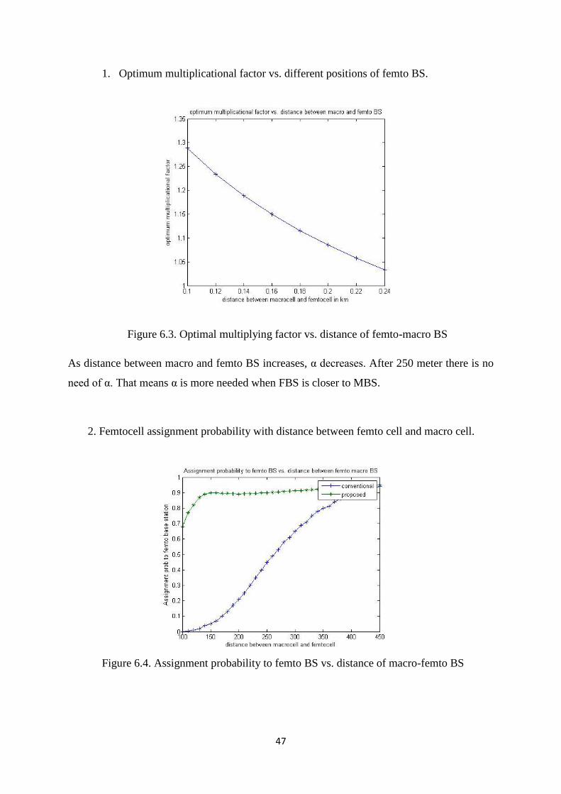
1. Optimum multiplicational factor vs. different positions of femto BS.

Figure 6.3. Optimal multiplying factor vs. distance of femto-macro BS

As distance between macro and femto BS increases, α decreases. After 250 meter there is no

need of α. That means α is more needed when FBS is closer to MBS.

2. Femtocell assignment probability with distance between femto cell and macro cell.

Figure 6.4. Assignment probability to femto BS vs. distance of macro-femto BS

48

When the femto BS is closely located to the macro BS, proposed algorithm has much

higher assignment probability to femto BS compared to conventional algorithm. It is

to be noted that each value is measured at the location separated by 10 m from the

femto BS.

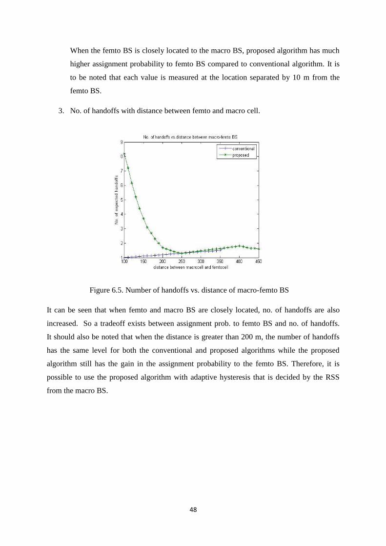
3. No. of handoffs with distance between femto and macro cell.

Figure 6.5. Number of handoffs vs. distance of macro-femto BS

It can be seen that when femto and macro BS are closely located, no. of handoffs are also

increased. So a tradeoff exists between assignment prob. to femto BS and no. of handoffs.

It should also be noted that when the distance is greater than 200 m, the number of handoffs

has the same level for both the conventional and proposed algorithms while the proposed

algorithm still has the gain in the assignment probability to the femto BS. Therefore, it is

possible to use the proposed algorithm with adaptive hysteresis that is decided by the RSS

from the macro BS.

49

Chapter 7.

Concluding remarks.

50

7.1. Conclusion.

First handoff scenarios in macro cell/femto cell coexisting network based on received

signal strength and SINR are observed using different indoor and outdoor path loss

models.

Interference and SINR are calculated in dense femto cell environment and their

effects on handover are obtained. Here we increased the number of femtocells in a

fixed area saw the effect on the interference and SINR considering no macrocell

interference to users. Interference increases with number of femtocells. Probability of

connection also increases.

Different handoff parameters like handover probability, RLF rate, ping –pong rate,

handover latency are evaluated in macro/femto handoff. Like handoff probability to

femto cell increases with increase of the number of femtocells. RLF and Ping-Pong

rate depends on hysteresis value and Time to trigger. There is a trade-off exist

between RLF and ping-pong rate. For reducing handover failures, we had to carefully

select the values of HM and TTT. Also handover latency is seen as a function of user

velocity.

Finally an algorithm is proposed for efficient handoff from macro cell to femto cell.

First it is seen how the value of α varies when the distance between macro cell and

femto cell is varied from 100 m to 1km. As the distance increases, the value of α

decreases and finally becomes 1. We can also see assignment probability to the FAP

is much higher after applying α when distance between macro cell and femto cell is

less which was our main objective. Then we had also shown the effect of α on the

number of handoffs in the network. Therefore it can be concluded that this proposed

algorithm gives much better performance in case of macro cell to femto cell handoff

scenario than conventional one.

51

Limitations.

Here we considered only one femto cell and one macro cell while applying this

algorithm. But practically the number of femtocells lying inside a macro cell is quite

large.

Sometimes due to introduction of the multiplying factor unnecessary handoffs take

place even though the received power from the target femto cell is not good enough.

Future scope of work.

As future works, system performance, such as utilization of femtocells and user

throughput, may be investigated when the proposed handoff decision algorithm is

used. Then, the derivation of optimal handoff location and the corresponding

application of the proposed algorithm can be examined. With more extensive analysis

and study, we are expecting that the proposed algorithm will give the desirable effects

on the improvement of the hierarchical macro/femto cell networks.

Also in real time scenario, using signal estimation, it can be examined how this

algorithm works and what the exact effect on handoff probability, assignment

probability to femto cell and number of handoffs are occurring.

52

7.2. BIBLIOGRAPHY.

[1] Jung-Min Moon “Efficient Handoff Algorithm for Inbound Mobility in

Hierarchical Macro/Femto Cell Networks” in IEEE COMMUNICATIONS

LETTERS, VOL. 13, NO. 10, pp. 755-757, OCTOBER 2009.

[2] K. Itoh et al., “Performance of Handoff Algorithm Based on Distance and RSSI

Measurements,” IEEE Transactions on Vehicular Technology, vol. 51, no. 6, pp.

1460-1468, November 2002.

[3] G. Pollini, “Trends in Handover Design,” IEEE Communications Magazine,vol. 34,

no. 3, pp. 82-90, March 1996.

[4] V. Chandrasekhar et al., “Femtocell Networks: A Survey,” IEEE

CommunicationsMagazine, vol. 46, no. 9, pp 59-67, September 2008.

[5] S. Moghaddam et al., “New Handoff Initiation Algorithm (Optimum Combination of

Hysteresis & Threshold Based Methods),” IEEE VehicularTechnology Conference

2000 Fall, pp. 1567-1574, September 2000.

[6] S. Yeh et al., “WiMAX Femtocells: A Perspective on Network Architecture,

Capacity and Coverage,” IEEE Communications Magazine, vol. 46, no. 10, pp. 58-65,

October 2008.

[7] H. Claussen, “Performance of macro- and co-channel femtocells in a hierarchical cell

structure,” in Proc. IEEE International Symposium on Personal, Indoor and Mobile

Radio Communications 2007, pp. 1–5, Sept.2007.

[8] M. Halgamuge et al., “Signal-based evaluation of handoff algorithms,” IEEE

Communication Letters, vol. 9, no. 9, pp. 790–792, Sept. 2005.

[9] Mohammad Alshami, “Femtocell interference and probability of connection in

different areas,” International journal of computing and digital systems 3, No. 1,

2014.

[10] Mustafa Zaman Chowdhury, “Handover management in high dense

femtocellular networks,”, EURASIP journal on wireless communication and

networking, 2013.

[11] Hyung Deng Bae, “Analysis of handover failures in LTE femtocell systems”.

[12] Zubin Rustam Bharucha, “Ad hoc wireless networks with femto cell

deployment: A study,”2010.

53

[13] Esra Aycan, “Interference scenarios and capacity performances for femtocell

networks,” International conference on Electrical and Electronics Engineering,

Turkey, December 2011.

[14] Ardian Ulvan, “Handover procedure and decision strategy in LTE based

femtocell networks,” Telecommunication systems 52, pp. 2733-2748, 2011.

[15] Femto Forum, http://www.femtoforum.org.

[16] Seoyun Jang, “Self optimization of single Femtocell coverage using handover

events in LTE systems,” Asia Pacific conference on Communications, 2011.

[17] Theodore S. Rappaport, “Wireless communications: Principles and practices,”.

[18] Dennis M.Rose, “Modelling of Femtocells- simulation of interference and

handover in LTE networks,” Vehicular Technology Conference, pp. 1-5, 2011.

[19] Yixue Lei, “Enhanced mobility state detection based mobility optimization for

Femto cells,” IET international conference, 2011.