Handbook of Moduli - Universiteit Utrechtfaber010/faberpandharipande.pdfon the moduli space of curves. Finally, we connect the boundary constructions in M 2,21 to the representation

Tautological and non-tautological cohomology of the modulispace of curves

C. Faber and R. Pandharipande

Abstract. After a short exposition of the basic properties of the tautological ringofMg,n, we explain three methods of detecting non-tautological classes in coho-mology. The first is via curve counting over finite fields. The second is by obtaininglength bounds on the action of the symmetric group Σn on tautological classes. Thethird is via classical boundary geometry. Several new non-tautological classes arefound.

Contents

0 Introduction . . . . . . . . . . . . . . . . . . . . . . . . . . . . . . . . . . . 2931 Tautological classes . . . . . . . . . . . . . . . . . . . . . . . . . . . . . . . 2952 Point counting and elliptic modular forms . . . . . . . . . . . . . . . . . . 3023 Point counting and Siegel modular forms . . . . . . . . . . . . . . . . . . 3074 Representation theory . . . . . . . . . . . . . . . . . . . . . . . . . . . . . . 3155 Boundary geometry . . . . . . . . . . . . . . . . . . . . . . . . . . . . . . . 322

0. Introduction

0.1. Overview

LetMg,n be the moduli space of Deligne-Mumford stable curves of genus gwith n marked points. The cohomology of Mg,n has a distinguished subring oftautological classes

RH∗(Mg,n) ⊂ H∗(Mg,n,Q)

studied extensively since Mumford’s seminal article [51]. While effective methodsfor exploring the tautological ring have been developed over the years, the structureof the non-tautological classes remains mysterious. Our goal here, after reviewingthe basic definitions and properties of RH∗(Mg,n) in Section 1, is to present threeapproaches for detecting and studying non-tautological classes.

2000 Mathematics Subject Classification. Primary 14H10; Secondary 14D10.Key words and phrases. Moduli, tautological classes, cohomology.

294 Tautological and non-tautological cohomology ofMg,n

We viewMg,n as a Deligne-Mumford stack. Not much is lost by considering thecoarse moduli space (if the automorphism groups are not forgotten). We encouragethe reader to take the coarse moduli point of view if stacks are unfamiliar.

0.2. Point counting and modular forms

Since the moduli space of Deligne-Mumford stable curves is defined over Z,reduction to finite fields Fq is well-defined. LetMg,n(Fq) denote the set of Fq-points.For various ranges of g, n, and q, counting the number of points ofMg,n(Fq) isfeasible. A wealth of information about H∗(Mg,n,Q) can be then obtained from theLefschetz fixed point formula applied to Frobenius.

The first examples where point counting reveals non-tautological cohomologyoccur in genus 1. The relationship between point counting and elliptic modularforms is discussed in Section 2. By interpreting the counting results in genus 2, aconjectural description of the entire cohomology ofM2,n has been found by Faberand van der Geer [19] in terms of Siegel modular forms. The formula is consistentwith point counting data for n 6 25. In fact, large parts of the formula have beenproven. The genus 2 results are presented in Section 3.

In genus 3, a more complicated investigation involving Teichmüller modularforms is required. The situation is briefly summarized in Section 3.7. As the genusincreases, the connection between point counting and modular forms becomes moredifficult to understand.

0.3. Representation theory

The symmetric group Σn acts onMg,n by permuting the markings. As a result,an Σn-representation on H∗(Mg,n,Q) is obtained.

Studying the Σn-action onH∗(Mg,n,Q) provides a second approach to the non-tautological cohomology. In Section 4, we establish an upper bound for the length1

of the irreducible Σn-representations occurring in the tautological ring R∗(Mg,n). Inmany cases, the bound is sharp. Assuming the conjectural formulas for H∗(M2,n,Q)

obtained by point counting, we find several classes of Hodge type which are pre-sumably algebraic (by the Hodge conjecture) but cannot possibly be tautological,because the length of the corresponding Σn-representations is too large. The firstoccurs inM2,21.

The proofs of the length bounds for the Σn-action on R∗(Mg,n) are obtainedby studying representations induced from the boundary strata. The strong vanishingof Proposition 2 of [23] with tautological boundary terms plays a crucial role in theargument.

1The number of parts in the corresponding partition.

C. Faber and R. Pandharipande 295

0.4. Boundary geometry

The existence of non-tautological cohomology classes of Hodge type was earlierestablished by Graber and Pandharipande [36]. In particular, an explicit such classin the boundary ofM2,22 was found. In Section 5, we revisit the non-tautologicalboundary constructions. The old examples are obtained in simpler ways and newexamples inM2,21 are found. The method is by straightforward intersection theoryon the moduli space of curves. Finally, we connect the boundary constructions inM2,21 to the representation investigation of Section 4.

0.5. Acknowledgements

We thank J. Bergström, C. Consani, G. van der Geer, T. Graber, and A. Pixtonfor many discussions related to the cohomology of the moduli space of curves.

C.F. was supported by the Göran Gustafsson foundation for research in naturalsciences and medicine and grant 622-2003-1123 from the Swedish Research Coun-cil. R.P. was partially supported by NSF grants DMS-0500187 and DMS-1001154.The paper was completed while R.P. was visiting the Instituto Superior Técnico inLisbon with support from a Marie Curie fellowship and a grant from the Gulbenkianfoundation.

1. Tautological classes

1.1. Definitions

LetMg,n be the moduli space of stable curves of genus g with nmarked pointsdefined over C. Let A∗(Mg,n,Q) denote the Chow ring. The system of tautologicalrings is defined2 to be the set of smallest Q-subalgebras of the Chow rings,

R∗(Mg,n) ⊂ A∗(Mg,n,Q),

satisfying the following two properties:

(i) The system is closed under push-forward via all maps forgetting markings:

π∗ : R∗(Mg,n)→ R∗(Mg,n−1).

(ii) The system is closed under push-forward via all gluing maps:

ι∗ : R∗(Mg1,n1∪{?})⊗Q R

∗(Mg2,n2∪{•})→ R∗(Mg1+g2,n1+n2),

ι∗ : R∗(Mg,n∪{?,•})→ R∗(Mg+1,n),

with attachments along the markings ? and •.While the definition appears restrictive, natural algebraic constructions typicallyyield Chow classes lying in the tautological ring.

2We follow here the definition of tautological classes in Chow given in [23]. Tautological classes incohomology are discussed in Section 1.7.


1.2. Basic examples

Consider first the cotangent line classes. For each marking i, let

Li →Mg,n

denote the associated cotangent line bundle. By definition

ψi = c1(Li) ∈ A1(Mg,n).

Let π denote the map forgetting the last marking,

(1.1) π :Mg,n+1 →Mg,n,

and let ι denote the gluing map,

ι :Mg,{1,2,...,i−1,?,i+1,...,n} ×M0,{•,i,n+1} −→Mg,n+1.

The Q-multiples of the fundamental classes [Mg,n] are contained in the tautologicalrings (as Q-multiples of the units in the subalgebras). A direct calculation shows:

−π∗

((ι∗([Mg,n]× [M0,3])

)2)= ψi.

Hence, the cotangent line classes lie in the tautological rings,

ψi ∈ R1(Mg,n) .

Consider next the κ classes defined via push-forward by the forgetful map (1.1),

κj = π∗(ψj+1n+1) ∈ A

j(Mg,n) .

Since ψn+1 has already been shown to be tautological, the κ classes are tautologicalby property (i),

κj ∈ Rj(Mg,n) .

The ψ and κ classes are very closely related.For a nodal curve C, let ωC denote the dualizing sheaf. The Hodge bundle E

overMg,n is the rank g vector bundle with fiber H0(C,ωC) over the moduli point

[C,p1, . . . ,pn] ∈Mg,n .

The λ classes are defined by

λk = ck(E) ∈ Ak(Mg,n) .

The Chern characters of E lie in the tautological ring by Mumford’s Grothendieck-Riemann-Roch computation [51]. Since the λ classes are polynomials in the Cherncharacters,

λk ∈ Rk(Mg,n) .

The ψ and λ classes are basic elements of the tautological ring R∗(Mg,n) arisingvery often in geometric constructions and calculations. The ψ integrals,

(1.2)∫Mg,n

ψa11 · · ·ψ

ann ,


can be evaluated by KdV constraints due to Witten and Kontsevich [45, 65]. Othergeometric approaches to the ψ integrals can be found in [49, 52]. In genus 0, thesimple formula ∫

M0,n

ψa11 · · ·ψ

ann =

(n− 3

a1, . . . ,an

)holds. Non-integer values occur for the first time in genus 1,∫

M1,1

ψ1 =124

.

Hodge integrals, when the λ classes are included,∫Mg,n

ψa11 · · ·ψ

ann λb1

1 . . . λbgg ,

can be reduced to ψ integrals (1.2) by Mumford’s Grothendieck-Riemann-Rochcalculation. An example of a Hodge integral evaluation3 is

(1.3)∫Mg

λ3g−1 =|B2g|

2g|B2g−2|

2g− 21

(2g− 2)!

The proof of (1.3) and several other exact formulas for Hodge integrals can be foundin [20].

1.3. Strata

The boundary strata of the moduli spaces of curves correspond to stable graphs

A = (V ,H,L,g : V → Z>0,a : H→ V , i : H→ H)

satisfying the following properties:

(1) V is a vertex set with a genus function g,(2) H is a half-edge set equipped with a vertex assignment a and fixed point

free involution i,(3) E, the edge set, is defined by the orbits of i in H,(4) (V ,E) define a connected graph,(5) L is a set of numbered legs attached to the vertices,(6) For each vertex v, the stability condition holds:

2g(v) − 2+ n(v) > 0,

where n(v) is the valence of A at v including both half-edges and legs.

The data of the topological type of a generic curve in a boundary stratum of themoduli space is recorded in the stable graph.

Let A be a stable graph. The genus of A is defined by

g =∑v∈V

g(v) + h1(A).

3Here, B2g denotes the Bernoulli number.


Define the moduli spaceMA by the product

MA =∏

v∈V(A)

Mg(v),n(v).

There is a canonical morphism4

ξA :MA →Mg,n

with image equal to the boundary stratum associated to the graph A. By repeateduse of property (ii),

ξA∗[MA] ∈ R∗(Mg,n) .

We can now describe a set of additive generators for R∗(Mg,n). LetA be a stablegraph of genus g with n legs. For each vertex v of A, let

θv ∈ R∗(Mg(v),n(v))

be an arbitrary monomial in the ψ and κ classes of the vertex moduli space. Thefollowing result is proven in [36].

Theorem 1.4. R∗(Mg,n) is generated additively by classes of the form

ξA∗

( ∏v∈V(A)

θv

).

By the dimension grading, the list of generators provided by Theorem 1.4 isfinite. Hence, we obtain the following result.

Corollary 1.5. We have dimQ R∗(Mg,n) <∞.

1.4. Further properties

The following two formal properties of the full system of tautological rings

R∗(Mg,n) ⊂ A∗(Mg,n,Q),

are a consequence of properties (i) and (ii):

(iii) The system is closed under pull-back via the forgetting and gluing maps.(iv) R∗(Mg,n) is an Sn-module via the permutation action on the markings.

Property (iii) follows from the well-known boundary geometry of the modulispace of curves. A careful treatment using the additive basis of Theorem 1.4 canbe found in [36]. The meaning of property (iii) for the reducible gluing is that theKünneth components of the pull-backs of tautological classes are tautological. Sincethe defining properties (i) and (ii) are symmetric with respect to the marked points,property (iv) holds.

4 To construct ξA, a family of stable pointed curves overMA is required. Such a family is easilydefined by attaching the pull-backs of the universal families over each of theMg(v),n(v) along the sections

corresponding to half-edges.


1.5. Pairing

Intersection theory on the moduli spaceMg,n yields a canonical pairing

µ : Rk(Mg,n)× R3g−3+n−k(Mg,n)→ Q

defined by

µ(α,β) =∫Mg,n

α ∪ β .

While the pairing µ has been speculated to be perfect in [21, 38, 53], very few resultsare known.

The pairing µ can be effectively computed on the generators of Theorem 1.4by the following method. The pull-back property (iii) may be used repeatedly toreduce the calculation of µ on the generators to integrals of the form∫

Mh,m

ψa11 · · ·ψ

amm · κb1

1 · · · κbrr .

The κ classes can be removed to yield a sum of purely ψ integrals∫Mh,m+r

ψa11 · · ·ψ

am+rm+r ,

see [3]. As discussed in Section 1.2, the ψ integrals can be evaluated by KdV con-straints.

1.6. Further examples

We present here two geometric constructions which also yield tautologicalclasses. The first is via stable maps and the second via moduli spaces of Hurwitzcovers.

Let X be a nonsingular projective variety, and let Mg,n(X,β) be the modulispace of stable maps5 representing β ∈ H2(X,Z). Let ρ denote the map to the moduliof curves,

ρ :Mg,n(X,β)→Mg,n.

The moduli spaceMg,n(X,β) carries a virtual class

[Mg,n(X,β)]vir ∈ A∗(Mg,n(X,β))

obtained from the canonical obstruction theory of maps.

Theorem 1.6. Let X be a nonsingular projective toric variety. Then,

ρ∗[Mg,n(X,β)]vir ∈ R∗(Mg,n).

5We refer the reader to [27] for an introduction to the subject. A discussion of obstruction theoriesand virtual classes can be found in [4, 5, 47].


The proof follows directly from the virtual localization formula of [35]. If[C] ∈Mg is a general moduli point, then

ρ∗[Mg(C,1)]vir = [C] ∈ A3g−3(Mg).

Since not all of A3g−3(Mg) is expected to be tautological, Theorem 1.6 is unlikelyto hold for C. However, the result perhaps holds for a much more general class ofvarieties X. In fact, we do not know6 any nonsingular projective variety defined overQ for which Theorem 1.6 is expected to be false.

The moduli spaces of Hurwitz covers of P1 also define natural classes on themoduli space of curves. Let µ1, . . . ,µm bem partitions of equal size d satisfying

2g− 2+ 2d =

m∑i=1

(d− `(µi)

),

where `(µi) denotes the length of the partition µi. The moduli space of Hurwitzcovers,

Hg(µ1, . . . ,µm)

parameterizes morphisms,

f : C→ P1,

whereC is a complete, connected, nonsingular curve with marked profiles µ1, . . . ,µm

overm ordered points of the target (and no ramifications elsewhere). The modulispace of Hurwitz covers is a dense open set of the compactmoduli space of admissiblecovers [39],

Hg(µ1, . . . ,µm) ⊂ Hg(µ1, . . . ,µm).

Let ρ denote the map to the moduli of curves,

ρ : Hg(µ1, . . . ,µm)→Mg,

∑mi=1 `(µ

i).

The following is a central result of [23].

Theorem 1.7. The push-forwards of the fundamental classes lie in the tautological ring,

ρ∗[Hg(µ1, . . . ,µm)] ∈ R∗(Mg,

∑mi=1 `(µ

i)) .

The admissible covers in Theorem 1.7 are of P1. The moduli spaces of admissi-ble covers of higher genus targets can lead to non-tautological classes [36].

6 We do not know any examples at all of nonsingular projective X where

ρ∗[Mg,n(X,β)]vir /∈ RH∗(Mg,n).

See [46] for a discussion.


1.7. Tautological rings

The tautological subrings

(1.8) RH∗(Mg,n) ⊂ H∗(Mg,n,Q)

are defined to be the images of R∗(Mg,n) under the cycle class map

A∗(Mg,n,Q)→ H∗(Mg,n,Q) .

The tautological rings RH∗(Mg,n) could alternatively be defined as the smallestsystem of subalgebras (1.8) closed under push-forward by all forgetting and gluingmaps (properties (i) and (ii)). Properties (iii) and (iv) also hold for RH∗(Mg,n).

Tautological rings in Chow and cohomology may be defined for all stages ofthe standard moduli filtration:

(1.9) Mg,n ⊃Mcg,n ⊃Mrt

g,n.

Here,Mcg,n is the moduli space of stable curves of compact type (curves with tree

dual graphs, or equivalently, with compact Jacobians), andMrtg,n is the moduli space

of stable curves with rational tails (the preimage of the moduli space of nonsingularcurvesMg ⊂Mg). The tautological rings

R∗(Mcg,n) ⊂ A∗(Mc

g,n,Q), RH∗(Mcg,n) ⊂ H∗(Mc

g,n,Q),

R∗(Mrtg,n) ⊂ A∗(Mrt

g,n,Q), RH∗(Mrtg,n) ⊂ H∗(Mrt

g,n,Q)

are all defined as the images of R∗(Mg,n) under the natural restriction and cycle classmaps.

Of all the tautological rings, the most studied case by far is R∗(Mg). A complete(conjectural) structure of R∗(Mg) is proposed in [18] with important advances madein [42, 48, 50]. Conjectures for the compact type cases R∗(Mc

g,n) can be found in[21]. See [22, 54] for positive results for compact type. Tavakol [59, 60] has recentlyproved that R∗(Mc

1,n) and R∗(Mrt

2,n) are Gorenstein, with socles in degrees n− 1 andn, respectively.

1.8. Hyperelliptic curves

As an example, we calculate the class of the hyperelliptic locus

Hg ⊂Mg

following [51].Over the moduli point [C,p] ∈Mg,1 there is a canonical map

φ : H0(C,ωC)→ H0(C,ωC/ωC(−2p))

defined by evaluating sections of ωC at the marking p ∈ C. If we define J to be therank 2 bundle overMg,1 with fiber H0(C,ωC/ωC(−2p)) over [C,p], then we obtaina morphism

φ : E→ J


overMg,1. By classical curve theory, the map φ fails to be surjective precisely whenC is hyperelliptic and p ∈ C is a Weierstrass point. Let

∆ ⊂Mg,1

be the degeneracy locus of φ of pure codimension g − 1. By the Thom-Porteousformula [26],

[∆] =

(c(E∗)c(J∗)

)g−1

.

By using the jet bundle sequence

0→ L21 → J→ L1 → 0,

we conclude

[∆] =

(1− λ1 + λ2 − λ3 + . . .+ (−1)gλg

(1−ψ1)(1− 2ψ1)

)g−1∈ Rg−1(Mg,1) .

To find a formula for the hyperelliptic locus, we view

π :Mg,1 →Mg

as the universal curve over moduli space. Since each hyperelliptic curve has 2g+ 2Weierstrass points,

[Hg] =1

2g+ 2π∗([∆]) ∈ Rg−2(Mg) .

By Theorem 1.7, the class of the closure of the hyperelliptic locus is also tautological,

[Hg] ∈ Rg−2(Mg),

but no simple formula is known to us.

2. Point counting and elliptic modular forms

2.1. Elliptic modular forms

We present here an introduction to the close relationship between modularforms and the cohomology of moduli spaces. The connection is most direct betweenelliptic modular forms and moduli spaces of elliptic curves.

Classically, a modular form is a holomorphic function f on the upper halfplane

H = {z ∈ C : Im z > 0}

with an amazing amount of symmetry. Precisely, a modular form of weight k ∈ Zsatisfies the functional equation

f

(az+ b

cz+ d

)= (cz+ d)kf(z)

for all z ∈ H and all(a bc d

)∈ SL(2,Z). By the symmetry for

(−1 00 −1

),

f(z) = (−1)kf(z),


so kmust be even. Using ( 1 10 1 ), we see

f(z+ 1) = f(z),

so f can be written as a function of q = exp(2πiz). We further require f to beholomorphic at q = 0. The Fourier expansion is

f(q) =

∞∑n=0

anqn.

If a0 vanishes, f is called a cusp form (of weight k for SL(2,Z)).Well-known examples of modular forms are the Eisenstein series7

Ek(q) = 1−2kBk

∞∑n=1

σk−1(n)qn

of weight k > 4 and the discriminant cusp form

(2.1) ∆(q) =

∞∑n=1

τ(n)qn = q

∞∏n=1

(1− qn)24

of weight 12 with the Jacobi product expansion (defining the Ramanujan τ-function).In both of the above formulas, the right sides are the Fourier expansions.

Let Mk be the vector space of holomorphic modular forms of weight k forSL(2,Z). The ring of modular forms is freely generated [44, Exc. III.2.5] by E4 and E6,∞⊕

k=0

Mk = C[E4,E6] ,

and the ideal⊕k Sk of cusp forms is generated by ∆. Let mk = dim Mk and

sk = mk − 1.For every positive integer n, there exists a naturally defined Hecke operator

Tn :Mk →Mk .

The Tn commute with each other and preserve the subspace Sk. Moreover, Sk has abasis of simultaneous eigenforms, which are orthogonal with respect to the Peterssoninner product and can be normalized to have a1 = 1. The Tn-eigenvalue of such aneigenform equals its n-th Fourier coefficient [44, Prop. III.40].

2.2. Point counting in genus 1

While the moduli spaceM1,1 of elliptic curves can be realized over C as theanalytic space H/SL(2,Z), we will viewM1,1 here as an algebraic variety over a fieldk or a stack over Z.

Over k, the j-invariant classifies elliptic curves, so

M1,1∼=k A1

7 Recall the Bernoulli numbers Bk are given by xex−1 =

∑Bk

xk

k! and σm(n) is the sum of them-th

powers of the positive divisors of n.


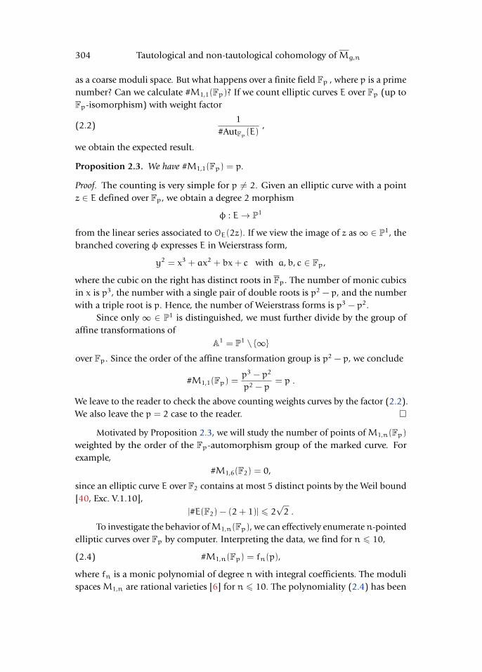
as a coarse moduli space. But what happens over a finite field Fp , where p is a primenumber? Can we calculate #M1,1(Fp)? If we count elliptic curves E over Fp (up toFp-isomorphism) with weight factor

(2.2)1

#AutFp(E),

we obtain the expected result.

Proposition 2.3. We have #M1,1(Fp) = p.

Proof. The counting is very simple for p 6= 2. Given an elliptic curve with a pointz ∈ E defined over Fp, we obtain a degree 2 morphism

φ : E→ P1

from the linear series associated to OE(2z). If we view the image of z as ∞ ∈ P1, thebranched covering φ expresses E in Weierstrass form,

y2 = x3 + ax2 + bx+ c with a,b, c ∈ Fp,

where the cubic on the right has distinct roots in Fp. The number of monic cubicsin x is p3, the number with a single pair of double roots is p2 − p, and the numberwith a triple root is p. Hence, the number of Weierstrass forms is p3 − p2.

Since only ∞ ∈ P1 is distinguished, we must further divide by the group ofaffine transformations of

A1 = P1 \ {∞}

over Fp. Since the order of the affine transformation group is p2 − p, we conclude

#M1,1(Fp) =p3 − p2

p2 − p= p .

We leave to the reader to check the above counting weights curves by the factor (2.2).We also leave the p = 2 case to the reader. �

Motivated by Proposition 2.3, we will study the number of points ofM1,n(Fp)weighted by the order of the Fp-automorphism group of the marked curve. Forexample,

#M1,6(F2) = 0,

since an elliptic curve E over F2 contains at most 5 distinct points by the Weil bound[40, Exc. V.1.10],

|#E(F2) − (2+ 1)| 6 2√2 .

To investigate the behavior ofM1,n(Fp), we can effectively enumeraten-pointedelliptic curves over Fp by computer. Interpreting the data, we find for n 6 10,

(2.4) #M1,n(Fp) = fn(p),

where fn is a monic polynomial of degree n with integral coefficients. The modulispacesM1,n are rational varieties [6] for n 6 10. The polynomiality (2.4) has been


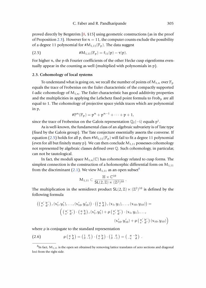
proved directly by Bergström [8, §15] using geometric constructions (as in the proofof Proposition 2.3). However for n = 11, the computer counts exclude the possibilityof a degree 11 polynomial for #M1,11(Fp). The data suggest

(2.5) #M1,11(Fp) = f11(p) − τ(p).

For higher n, the p-th Fourier coefficients of the other Hecke cusp eigenforms even-tually appear in the counting as well (multiplied with polynomials in p).

2.3. Cohomology of local systems

To understand what is going on, we recall the number of points ofM1,n over Fpequals the trace of Frobenius on the Euler characteristic of the compactly supported`-adic cohomology ofM1,n. The Euler characteristic has good additivity propertiesand the multiplicities in applying the Lefschetz fixed point formula to Frobp are allequal to 1. The cohomology of projective space yields traces which are polynomialin p,

#Pn(Fp) = pn + pn−1 + · · ·+ p+ 1,

since the trace of Frobenius on the Galois representation Q`(−i) equals pi.As is well-known, the fundamental class of an algebraic subvariety is of Tate type

(fixed by the Galois group). The Tate conjecture essentially asserts the converse. Ifequation (2.5) holds for all p, then #M1,11(Fp) will fail to fit a degree 11 polynomial(even for all but finitely many p). We can then concludeM1,11 possesses cohomologynot represented by algebraic classes defined over Q. Such cohomology, in particular,can not be tautological.

In fact, the moduli spaceM1,n(C) has cohomology related to cusp forms. Thesimplest connection is the construction of a holomorphic differential form onM1,11

from the discriminant (2.1). We viewM1,11 as an open subset8

M1,11 ⊂H× C10

SL(2,Z)n (Z2)10.

The multiplication in the semidirect product SL(2,Z)n (Z2)10 is defined by thefollowing formula((

a′ b′

c′ d′

), (x ′1,y

′1), . . . , (x

′10,y

′10))·((a bc d

), (x1,y1), . . . , (x10,y10)

)=( (

a′ b′

c′ d′

)·(a bc d

), (x ′1,y

′1) + ρ

(a′ b′

c′ d′

)· (x1,y1), . . . ,

(x ′10,y′10) + ρ

(a′ b′

c′ d′

)(x10,y10)

)where ρ is conjugate to the standard representation

(2.6) ρ(a bc d

)=(1 00 −1

)·(a bc d

)·(1 00 −1

)=(a −b

−c d

).

8In fact,M1,11 is the open set obtained by removing lattice translates of zero sections and diagonalloci from the right side.


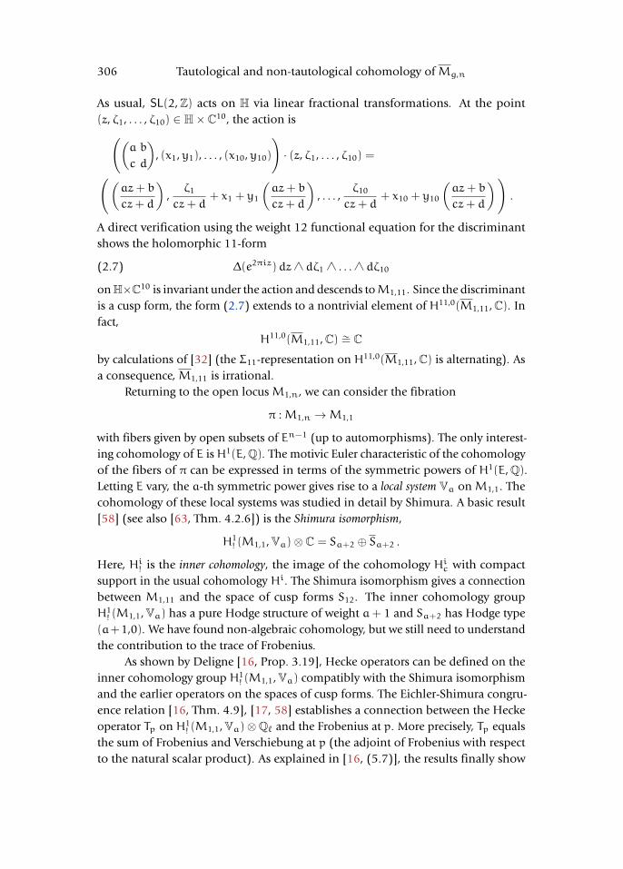
As usual, SL(2,Z) acts on H via linear fractional transformations. At the point(z, ζ1, . . . , ζ10) ∈ H× C10, the action is((

a b

c d

), (x1,y1), . . . , (x10,y10)

)· (z, ζ1, . . . , ζ10) =((

az+ b

cz+ d

),ζ1

cz+ d+ x1 + y1

(az+ b

cz+ d

), . . . ,

ζ10

cz+ d+ x10 + y10

(az+ b

cz+ d

)).

A direct verification using the weight 12 functional equation for the discriminantshows the holomorphic 11-form

(2.7) ∆(e2πiz)dz∧ dζ1 ∧ . . .∧ dζ10

onH×C10 is invariant under the action and descends toM1,11. Since the discriminantis a cusp form, the form (2.7) extends to a nontrivial element of H11,0(M1,11,C). Infact,

H11,0(M1,11,C) ∼= C

by calculations of [32] (the Σ11-representation on H11,0(M1,11,C) is alternating). Asa consequence,M1,11 is irrational.

Returning to the open locusM1,n, we can consider the fibration

π :M1,n →M1,1

with fibers given by open subsets of En−1 (up to automorphisms). The only interest-ing cohomology of E isH1(E,Q). The motivic Euler characteristic of the cohomologyof the fibers of π can be expressed in terms of the symmetric powers of H1(E,Q).Letting E vary, the a-th symmetric power gives rise to a local system Va onM1,1. Thecohomology of these local systems was studied in detail by Shimura. A basic result[58] (see also [63, Thm. 4.2.6]) is the Shimura isomorphism,

H1! (M1,1,Va)⊗ C = Sa+2 ⊕ Sa+2 .

Here, Hi! is the inner cohomology, the image of the cohomology Hic with compactsupport in the usual cohomology Hi. The Shimura isomorphism gives a connectionbetween M1,11 and the space of cusp forms S12. The inner cohomology groupH1

! (M1,1,Va) has a pure Hodge structure of weight a+ 1 and Sa+2 has Hodge type(a+1,0). We have found non-algebraic cohomology, but we still need to understandthe contribution to the trace of Frobenius.

As shown by Deligne [16, Prop. 3.19], Hecke operators can be defined on theinner cohomology group H1

! (M1,1,Va) compatibly with the Shimura isomorphismand the earlier operators on the spaces of cusp forms. The Eichler-Shimura congru-ence relation [16, Thm. 4.9], [17, 58] establishes a connection between the Heckeoperator Tp on H1

! (M1,1,Va)⊗Q` and the Frobenius at p. More precisely, Tp equalsthe sum of Frobenius and Verschiebung at p (the adjoint of Frobenius with respectto the natural scalar product). As explained in [16, (5.7)], the results finally show


the trace of Frobenius at p on H1! (M1,1,Va) ⊗ Q` to be equal to the trace of the

Hecke operator Tp on Sa+2, which is the sum of the p-th Fourier coefficients of thenormalized Hecke cusp eigenforms.

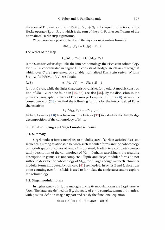
We are now in a position to derive the mysterious counting formula

#M1,11(Fp) = f11(p) − τ(p).

The kernel of the map

Hic(M1,1,Va)→ Hi(M1,1,Va)

is the Eisenstein cohomology. Like the inner cohomology, the Eisenstein cohomologyfor a > 0 is concentrated in degree 1. It consists of Hodge-Tate classes of weight 0which over C are represented by suitably normalized Eisenstein series. WritingS[a+ 2] for H1

! (M1,1,Va), we obtain

(2.8) ec(M1,1,Va) = −S[a+ 2] − 1

for a > 0 even, while the Euler characteristic vanishes for a odd. A motivic construc-tion of S[a + 2] can be found in [15, 57], see also [56]. By the discussion in theprevious paragraph, the trace of Frobenius picks up −τ(p) from (2.8). As anotherconsequence of (2.8), we find the following formula for the integer valued Eulercharacteristic,

Ec(M1,1,Va) = −2sa+2 − 1.

In fact, formula (2.8) has been used by Getzler [32] to calculate the full Hodgedecomposition of the cohomology ofM1,n.

3. Point counting and Siegel modular forms

3.1. Summary

Siegel modular forms are related to moduli spaces of abelian varieties. As a con-sequence, a strong relationship between such modular forms and the cohomologyof moduli spaces of curves of genus 2 is obtained, leading to a complete (conjec-tural) description of the cohomology ofM2,n. Perhaps surprisingly, the resultingdescription in genus 3 is not complete. Elliptic and Siegel modular forms do notsuffice to describe the cohomology ofM3,n for n large enough — the Teichmüllermodular forms introduced by Ichikawa [41] are needed. In genus 2 and 3, data frompoint counting over finite fields is used to formulate the conjectures and to explorethe cohomology.

3.2. Siegel modular forms

In higher genus g > 1, the analogue of elliptic modular forms are Siegel modularforms. The latter are defined on Hg, the space of g× g complex symmetric matriceswith positive-definite imaginary part and satisfy the functional equation

f((az+ b)(cz+ d)−1) = ρ(cz+ d)f(z)


for all z ∈ Hg and all(a bc d

)∈ Sp(2g,Z). Here, ρ is a representation of GL(g,C).

Classically,

ρ(M) = Detk(M),

but other irreducible representations of GL(g,C) are just as relevant. The form f isvector valued. Since z has positive definite imaginary part, cz+d is indeed invertible.

Hecke operators can be defined on Siegel modular forms [1, 2]. The Fouriercoefficients of an eigenform here contain much more information than just theHecke eigenvalues:

(i) the coefficients are indexed by positive semi-definite g× g symmetric matri-ces with integers on the diagonal and half-integers elsewhere,

(ii) the coefficients themselves are vectors.

Cusp forms are Siegel modular forms in the kernel of the Siegel Φ-operator:

(Φf)(z ′) = limt→∞ f

(z′ 00 it

),

for z ′ ∈ Hg−1. As before, the Hecke operators preserve the space of cusp forms.

3.3. Point counting in genus 2

Since genus 2 curves are double covers of P1, we can effectively count themover Fp. As before, each isomorphism class over Fp is counted with the reciprocal ofthe number of Fp-automorphisms. For small n, the enumeration ofM2,n(Fp) canbe done by hand as in Proposition 2.3. For large n, computer counting is needed.

Bergström [9] has proven the polynomiality in p of #M2,n(Fp) for n 6 7 bygeometric stratification of the moduli space. Experimentally, we find #M2,n(Fp) is apolynomial of degree n+ 3 in p for n 6 9. In the range 10 6 n 6 13, the functionτ(p) multiplied by a polynomial appears in #M2,n(Fp). More precisely, computercounting predicts

#M2,10(Fp) = f13(p) + (p− 9)τ(p) .

If the above formula holds, then the possibility of a degree 13 polynomial for#M2,10(Fp) is excluded, so we concludeM2,10 has cohomology which is not algebraicover Q (and therefore non-tautological).

Higher weight modular forms appear in the counting for n = 14. Computercounts predict

#M2,14(Fp) = f17(p) + f5(p)τ(p) − 13c16(p) − 429c18(p),

where c16(p) and c18(p) are the Fourier coefficients of the normalized Hecke cuspeigenforms of weights 16 and 18. The appearance of c16(p) is perhaps not sosurprising since

τ = c12

occurs in the function #M2,10(Fp). By counting Σ14-equivariantly, we find the coef-ficient 13 arises as the dimension of the irreducible representation corresponding


to the partition [2112] (the tensor product of the standard representation and thealternating representation).

More surprising is the appearance of c18(p). Reasoning as before in Section 2.2,we would expect the motive S[18] to occur in the cohomology ofM2,14. Since theHodge types are (17,0) and (0,17), the motive S[18] cannot possibly come from theboundary of the 17 dimensional moduli space, but must come from the interior.We would then expect a Siegel cusp form to be responsible for the occurrence, withHecke eigenvalues closely related to those of the elliptic cusp form of weight 18.There indeed exists such a Siegel modular form: the classical Siegel cusp form χ10

of weight 10, the product of the squares of the 10 even theta characteristics, is aSaito-Kurokawa lift of E6∆. In particular, the Hecke eigenvalues are related via

λχ10(p) = λE6∆(p) + p8 + p9 = c18(p) + p

8 + p9.

The coefficient 429 is the dimension of the irreducible representation correspondingto the partition [27], as a Σ14-equivariant count shows.

The function #M2,15(Fp) is expressible in terms of τ, c16, and c18 as expected.For n = 16, the Hecke eigenvalues of a vector valued Siegel cusp form appear for thefirst time: the unique form of type

ρ = Sym6 ⊗Det8

constructed by Ibukiyama (see [19]) arises. For n 6 25, the computer counts of#M2,n(Fp) have to a large extent been successfully fit by Hecke eigenvalues of Siegelcusp forms [37].

3.4. Local systems in genus 2

To explain the experimental results for #M2,n(Fp) discussed above, we studythe cohomology of local systems on the moduli spaceM2. Via the Jacobian, there isan inclusion

M2 ⊂ A2

as an open subset in the moduli space of principally polarized abelian surfaces. Infact, the geometry of local systems on A2 is a more natural object of study.

The irreducible representations Va,b of Sp(4,Z) are indexed by integers

a > b > 0.

More precisely, Va,b is the irreducible representation of highest weight occurring inSyma−b(R)⊗ Symb(∧2R), where R is the dual of the standard representation. Sincethe moduli space of abelian surfaces arises as a quotient,

A2 = H2/Sp(4,Z),

we obtain local systems Va,b for Sp(4,Z) on A2 associated to the representationsVa,b. The local system Va,b is regular if a > b > 0.


Faltings and Chai [25, Thm. VI.5.5] relate the cohomology of Va,b on A2 to thespace Sa−b,b+3 of Siegel cusp forms of type Syma−b⊗Detb+3. To start,Hic(A2,Va,b)has a natural mixedHodge structure with weights at most a+ b+ i, andHi(A2,Va,b)has a mixed Hodge structure with weights at least a+ b+ i. The inner cohomologyHi!(A2,Va,b) therefore has a pure Hodge structure of weight a+ b+ i. Faltings [24,Cor. of Thm. 9] had earlier shown that Hi!(A2,Va,b) is concentrated in degree 3when the local system is regular. For the Hodge structures above, the degrees of theHodge filtration are contained in

{0,b+ 1,a+ 2,a+ b+ 3}.

Finally, there are natural isomorphisms

Fa+b+3H3(A2,Va,b) ∼=Ma−b,b+3,

Fa+b+3H3c(A2,Va,b) = Fa+b+3H3

! (A2,Va,b) ∼= Sa−b,b+3

with the spaces of Siegel modular (respectively cusp) forms of the type mentionedabove. The quotients in the Hodge filtration are isomorphic to certain explicitcoherent cohomology groups, see [31, Thm. 17].

One is inclined to expect the occurrence of motives S[a− b,b+ 3] correspond-ing to Siegel cusp forms in H3

! (A2,Va,b), at least in the case of a regular weight.Each Hecke cusp eigenform should contribute a 4-dimensional piece with four1-dimensional pieces in the Hodge decomposition of types

(a+ b+ 3,0), (a+ 2,b+ 1), (b+ 1,a+ 2), (0,a+ b+ 3).

By the theory of automorphic representations, the inner cohomology may containother terms as well, the so-called endoscopic contributions. In the present case, theendoscopic contributions come apparently only9 with Hodge types (a+ 2,b+ 1)and (b+ 1,a+ 2).

Based on the results from equivariant point counts, Faber and van der Geer[19] obtain the following explicit conjectural formula for the Euler characteristic ofthe compactly supported cohomology:

Conjecture. For a > b > 0 and a+ b even,

ec(A2,Va,b) = −S[a− b,b+ 3] − sa+b+4S[a− b+ 2]Lb+1

+ sa−b+2 − sa+b+4Lb+1 − S[a+ 3] + S[b+ 2] + 1

2 (1+ (−1)a).

The terms in the second line constitute the Euler characteristic of the Eisensteincohomology. The second term in the first line is the endoscopic contribution. Justas in the genus 1 case, the hyperelliptic involution causes the vanishing of all co-homology when a+ b is odd. However, the above conjecture is not quite a precise

9However, our use of the term endoscopic is potentially non-standard.


statement. While L is the Lefschetz motive and S[k] has been discussed in Section2.3, the motives S[a− b,b+ 3] have not been constructed yet. Nevertheless, severalprecise predictions of the conjecture will be discussed.

First, we can specialize the conjecture to yield a prediction for the integer valuedEuler characteristic Ec(A2,Va,b) . The formula from the conjecture is

Ec(A2,Va,b) = −4sa−b,b+3 − 2sa+b+4sa−b+2

+ sa−b+2 − sa+b+4 − 2sa+3 + 2sb+2 +12 (1+ (−1)a).

for a > b > 0 and a + b even. The lower case s denotes the dimension of thecorresponding space of cusp forms. The dimension formula was proved by Grundh[37] for b > 1 using earlier work of Getzler [33] and a formula of Tsushima [61] forsj,k, proved for k > 4 (and presumably true for k = 4). In fact, combining work ofWeissauer [64] on the inner cohomology and of van der Geer [28] on the Eisensteincohomology, one may deduce the implication of the conjecture obtained by takingthe realizations as `-adic Galois representations of all terms.

A second specialization of the conjecture yields a prediction for #M2,n(Fp) viathe eigenvalues of Hecke cusp forms. The prediction has been checked forn 6 17 andp 6 23. The prediction for the trace of Frobp on ec(M2,Va,b) has been checked inmany more cases. Consider the local systems Va,b with a+ b 6 24 and b > 5. Thereare 13 such local systems with dimSa−b,b+3 = 1; the prediction has been checked for11 of them, for p 6 23. There are also 6 such local systems with dimSa−b,b+3 = 2,the maximal dimension; the prediction has been checked for all 6 of them, forp 6 17.

We believe the conjecture to be correct also when a = b or b = 0 after a suitablere-interpretation of several terms. To start, we set s2 = −1 and define

S[2] = −L− 1,

which of course is not equal to H1! (M1,1,V0) but does yield the correct answer for

ec(M1,1,V0) = L.

Let S[k] = 0 for odd k. Similarly, define

S[0,3] = −L3 − L2 − L− 1 .

By analogy, let s0,3 = −1, which equals the value produced by Tsushima’s formula(the only negative value of sj,k for k > 3). We then obtain the correct answer for

ec(A2,V0,0) = L3 + L2.

Finally, S[0,10] is defined as L8+S[18] +L9, and more generally, S[0,m+1] includes(for m odd) a contribution SK[0,m + 1] defined as S[2m] + s2m(Lm−1 + Lm) —corresponding to the Saito-Kurokawa lifts, but not a part of H3

! (A2,Vm−2,m−2).


3.5. Holomorphic differential forms

We can use the Siegel modular form χ10 to construct holomorphic differentialforms onM2,14. To start, we consider the seventh fiber product U7 of the universalabelian surface

U→ A2 .

We can construct U7 as a quotient,

U7 =H2 × (C2)7

Sp(4,Z)n (Z4)7.

The semidirect product is defined by the conjugate of the standard representationfollowing (2.6). We will take z = ( z11 z12z12 z22 ) ∈ H2 and ζi = (ζi1, ζi2) ∈ C2 to becoordinates. At the point

(z, ζ1, . . . , ζ7) ∈ H2 × (C2)7,

the action is

((a bc d

), (x1,y1), . . . , (x7,y7)) · (z, ζ1, . . . , ζ7) =((az+ b)(cz+ d)−1, ζ1(cz+ d)−1 + x1 + y1(az+ b)(cz+ d)

−1,

. . . , ζ7(cz+ d)−1 + x7 + y7(az+ b)(cz+ d)−1),

where xi,yi ∈ Z2. A direct verification using the weight 10 functional equation forχ10 shows the holomorphic 17-form

(3.1) χ10(z)dz11 ∧ dz12 ∧ dz22 ∧ dζ11 ∧ dζ12 ∧ . . .∧ dζ71 ∧ dζ72

on H2 × (C2)7 is invariant under the action and descends to U7.To obtain a 17-form onM2,14, we consider the Abel-Jacobi mapM2,14 → U7

defined by

(C,p1, . . . ,p14) 7→ (Jac0(C),ω∗C(p1 + p2), . . . ,ω∗C(p13 + p14)) .

The pull-back of (3.1) yields a holomorphic 17-form onM2,14. Since χ10 is a cuspform, the pull-back extends to a nontrivial element of H17,0(M2,14,C). Assumingthe conjecture for local systems in genus 2,

H17,0(M2,14,C) ∼= C429

with Σ14-representation irreducible of type [27]. We leave as an exercise for the readerto show our construction of 17-forms naturally yields the representation [27].

The existence of 17-forms implies the irrationality ofM2,14. BothM2,n612 andthe quotient ofM2,13 obtained by unordering the last two points are rational byclassical constructions [14]. IsM2,13 rational?


3.6. The compactificationM2,n

We now assume the conjectural formula for ec(A2,Va,b) holds for a > b > 0.As a consequence, we can compute the Hodge numbers of the compactificationsM2,n for all n.

We view, as before,M2 ⊂ A2 via the Torelli morphism. The complement is iso-morphic to Sym2A1. The local systems Va,b can be pulled back toM2 and restrictedto Sym2A1. The cohomology of the restricted local systems can be understood bycombining the branching formula from Sp4 to SL2×SL2 with an analysis of the effectof quotienting by the involution of A1 ×A1 which switches the factors, [13, 37, 55].Hence, the Euler characteristic ec(M2,Va,b)may be determined. The motives ∧2S[k]

and Sym2S[k] (which sum to S[k]2) will occur. Note

∧2S[k] ∼= Lk−1

when sk = 1.As observed by Getzler [31], the Euler characteristics ec(M2,Va,b) for a+b 6 N

determine and are determined by the Σn-equivariant Euler characteristics eΣnc (M2,n)

for n 6 N. Hence, the latter are (conjecturally) determined for all n. Next, bythe work of Getzler and Kapranov [34], the Euler characteristics eΣnc (M2,n) aredetermined as well, since we know the Euler characteristics in genus at most 1.Conversely, the answers forM2,n determine those forM2,n. After implementing theGetzler-Kapranov formalism (optimized for genus 2), a calculation of eΣnc (M2,n)

for all n 6 22 has been obtained.10 All answers satisfy Poincaré duality, which is avery non-trivial check.

The cohomology ofM2,21 is of particular interest to us. The motives ∧2S[12]and Sym2S[12] appear for the first time for n = 21 (with a Tate twist). The coefficientof L∧2 S[12] in eΣ21

c (M2,21) equals

[3118] + [322 114] + [324 110] + [326 16] + [328 12] + [2119] + [22 117]

+ [23 115] + [24 113] + [25 111] + [26 19] + [27 17] + [28 15] + [29 13] + [210 11]

as a Σ21-representation. As mentioned,

(3.2) ∧2 S[12] ∼= L11.

We find thus 1939938 independent Hodge classes L12, which should be algebraic bythe Hodge conjecture. However, 1058148 of these classes come with an irreduciblerepresentation of length at least 13. By Theorem 4.2 obtained in Section 4, the latterclasses cannot possibly be tautological.

The 1058148 classes actually span a small fraction of the full cohomologyH12,12(M2,21). There are also

124334448501272723333691

10Thanks to Stembridge’s symmetric functions package SF.


classes L12 not arising via the isomorphism (3.2)— all the irreducible representationsof length at most 12 arise in the coefficients.

3.7. Genus 3

In recent work [11], Bergström, Faber, and van der Geer have extended thepoint counts of moduli spaces of curves over finite fields to the genus 3 case. For all(n1,n2,n3) and all prime powers q 6 17, the frequencies∑

C

1#AutFq(C)

have been computed, where we sum over isomorphism classes of curves C overFq with exactly ni points over Fqi . The Σn-equivariant counts #M3,n(Fq) are thendetermined.

The isomorphism classes of Jacobians of nonsingular curves of genus 3 forman open subset of the moduli space A3 of principally polarized abelian varieties ofdimension 3.11 The complement can be easily understood. Defining the Sp(6,Z)local systems Va,b,c in expected manner, the traces of Frobq on ec(M3,Va,b,c) andec(A3,Va,b,c) can be computed for q 6 17 and arbitrary a > b > c > 0.

Interpretation of the results has been quite successful for A3 : an explicit conjec-tural formula for ec(A3,Va,b,c) has been found in [11], compatible with all knownresults (the results of Faltings [24] and Faltings-Chai [25] mentioned above, thedimension formula for the spaces of classical Siegel modular forms [62], and thenumerical Euler characteristics [13, §8]). Two features of the formula are quitestriking. First, it has a simple structure in which the endoscopic and Eisensteincontributions for genus 2 play an essential role. Second, it predicts the existence ofmany vector valued Siegel modular forms that are lifts, connected to local systems ofregular weight12, see [11].

Interpreting the results forM3 is much more difficult. In fact, the stackM3

cannot be correctly viewed as an open part of A3. Rather,M3 is a (stacky) doublecover of the locus J3 of Jacobians of nonsingular curves, branched over the locus ofhyperelliptic Jacobians. The double covering occurs because

Aut(Jac0(C)) = Aut(C)× {±1}

for C a non-hyperelliptic curve, while equality of the automorphism groups holdsfor C hyperelliptic. As a result, the local systems Va,b,c of odd weight a + b + c

will in general have non-vanishing cohomology onM3, while their cohomologyon A3 vanishes. We therefore can not expect that the main part of the cohomologyof Va,b,c onM3 can be explained in terms of Siegel cusp forms when a + b + c isodd. On the other hand, the local systems of even weight provide no difficulties.

11For g > 4, Jacobians have positive codimension inAg.12An analogous phenomenon occurs for Siegel modular forms of genus 2 and level 2, see [10], §6.


Bergström [8] has proved that the Euler characteristics ec(M3,Va,b,c) are certainexplicit polynomials in L, for a+ b+ c 6 7.

In fact, calculations ([12], in preparation) show that motives not associatedto Siegel cusp forms must show up in ec(M3,V11,3,3) and ec(M3,V7,7,3), and there-fore in eΣ17

c (M3,17), with the irreducible representations of type [33 18] and [33 24].Teichmüller modular forms [41] should play an important role in accounting forthe cohomology in genus 3 not explained by Siegel cusp forms.

4. Representation theory

4.1. Length bounds

Consider the standard moduli filtration

Mg,n ⊃Mcg,n ⊃Mrt

g,n

discussed in Section 1.7. We consider only pairs g and n which satisfy the stabilitycondition

2g− 2+ n > 0 .

If g = 0, all three spaces are equal by definition

M0,n =Mc0,n =Mrt

0,n .

If g = 1, the latter two are equal

Mc1,n =Mrt

1,n .

For g > 2, all three are different.The symmetric group Σn acts on Mg,n by permuting the markings. Hence,

Σn-actions are induced on the tautological rings

(4.1) R∗(Mg,n), R∗(Mcg,n), R

∗(Mrtg,n) .

By Corollary 1.5, all the rings (4.1) are finite dimensional representations of Σn.We define the length of an irreducible representation of Σn to be the number

of parts in the corresponding partition of n. The trivial representation has length1, and the alternating representation has length n. We define the length `(V) of afinite dimensional representation V of Σn to be the maximum of the lengths of theirreducible constituents.

Our main result bounds the lengths of the tautological rings in all cases (4.1).

Theorem 4.2. For the tautological rings of the moduli spaces of curves, we have

(i) `(Rk(Mg,n)) 6 min(k+ 1,3g− 2+ n− k,

⌊ 2g−1+n2

⌋),

(ii) `(Rk(Mcg,n)) 6 min (k+ 1,2g− 2+ n− k),

(iii) `(Rk(Mrtg,n)) 6 min (k+ 1,g− 1+ n− k).


The length bounds in all cases are consistent with the conjectures of Poincaréduality for these tautological rings, see [18, 21, 38, 53]. For (i), the bound is invariantunder

k ←→ 3g− 3+ n− k .

For (ii), the bound is invariant under

k ←→ 2g− 3+ n− k

which is consistent with a socle in degree 2g−3+n. For (iii), the bound is invariantunder

k ←→ g− 2+ n− k

which is consistent with a socle in degree g− 2+ n (for g > 0).In genus g, the bound

⌊ 2g−1+n2

⌋in case (i) improves upon the trivial length

bound n only for n > 2g.

4.2. Induction

The proof of Theorem 4.2 relies heavily on a simple length property of inducedrepresentations of symmetric groups.

Let V1 and V2 be representations of Σn1 and Σn2 of lengths `1 and `2 respectively.For n = n1 + n2, we view

Σn1 × Σn2 ⊂ Σnin the natural way.

Proposition 4.3. We have `(Ind˚n

˚n1×˚n2V1 ⊗ V2

)= `1 + `2 .

Proof. To prove the result, wemay certainly assumeVi is an irreducible representationVλi . In fact, we will exchange Vλi for a representation more closely related toinduction.

For α = (α1, . . . ,αk) a partition of m, let Uα be the representation of Σminduced from the trivial representation of the Young subgroup

Σα = Σα1 × · · · × Σαkof Σm. Young’s rule expressesUλ in terms of irreducible representations Vµ for whichµ precedes λ in the lexicographic ordering,

(4.4) Uλ ∼= Vλ ⊕⊕µ>λ

KµλVµ .

The Kostka number Kµλ does not vanish if and only if µ dominates λ, which implies`(µ) 6 `(λ). Therefore Vλ−Uλ can be written in the representation ring as a Z-linearcombination of Uµ for which µ > λ and `(µ) 6 `(λ).

If we let V1 = Uλ1 and V2 = Uλ2 , the induction of representations is easy tocalculate,

IndΣn1+n2Σn1×Σn2

Uλ1 ⊗Uλ2 = IndΣn1+n2Σλ1×Σλ2

1 ∼= IndΣn1+n2Σλ1+λ2

1 = Uλ1+λ2 ,


where λ1 + λ2 is the partition of n consisting of the parts of λ1 and λ2, reordered.Hence, the Proposition is proven for Uλ1 and Uλ2 . By the decomposition (4.4), theProposition follows for Vλ1 and Vλ2 . �

4.3. Proof of Theorem 4.2

4.3.1. Genus 0 The genus 0 result

`(Rk(M0,n)) 6 min (k+ 1,n− k− 2)

plays an important role in the rest of the proof of Theorem 4.2 and will be provenfirst.

By Keel [43], we have isomorphisms

Ak(M0,n) = Rk(M0,n) = H

2k(M0,n).

Poincaré duality then implies

(4.5) `(Rk(M0,n)) = `(Rn−3−k(M0,n)) .

The vector space Rk(M0,n) is generated by strata classes of curves with k nodes (andhence with k+ 1 components). The bound

`(Rk(M0,n)) 6 k+ 1

follows by a repeated application of Proposition 4.3 or by observing

`(Uλ) = `(λ),

for any partition λ (here with at most k+ 1 parts). The bound

`(Rk(M0,n)) 6 n− k− 2

is obtained by using (4.5). �

4.3.2. Rational tails We prove next a length bound for the subrepresentations ofRk(Mg,n) generated by the decorated strata classes of curves with rational tails, inother words, by the classes

ξA∗

( ∏v∈V(A)

θv

)as in Theorem 1.4, where A is a stable graph of genus g > 1 with n legs and exactlyone vertex of genus g (and all other vertices of genus 0).

Let α be such a class of codimension k and graphA. Let v be the vertex of genusg. We may assume the decoration is supported only at v, so

α = ξA∗θv .

The graph A arises by attaching t rational trees Ti to v. Let Ti have (before attaching)ki edges andmi legs. Letm > t denote the valence of v. After attaching the trees, v


hasm− t legs. Of them− t legs, let s0 come without ψ class, s1 come with ψ1, s2come with ψ2, and so forth, so ∑

j

sj = m− t .

After discarding the sj which vanish, we obtain a partition ofm− t with p positiveparts. The m − t legs contribute a class ζv of degree

∑j jsj to θv. Let ηv be the

product of the κ classes at the vertex and the ψ classes at the t legs at which the treesare attached, so

θv = ζvηv .

Let e be the degree of ηv. We clearly have

k =∑i

ki + t+ e+∑j

jsj and n = m+∑i

mi − 2t.

At the vertex v, we obtain a representation of Σm−t of length p. By the resultfor genus 0, each tree Ti generates a subrepresentation Vi of Rki(M0,mi) with

`(Vi) 6 min(ki + 1,mi − ki − 2).

One of themi legs is used in attaching Ti to v. After restricting Vi to Σmi−1, the lengthcan only decrease. Applying Proposition 4.3, we see α generates a subrepresentationV of Rk(Mg,n) with

`(V) 6 p+∑i

min(ki + 1,mi − ki − 2).

Taking the first terms in the minimum expressions, we have

(4.6) `(V) 6 p+∑i

(ki + 1) = p+ k− e−∑j

jsj .

Since ∑j

jsj =∑

j>1:sj>0

jsj >∑

j>1:sj>0

1 = p− 1+ δs0,0 ,

we seep−

∑j

jsj 6 1− δs0,0 6 1 .

After substituting in (4.6) and using e > 0, we conclude

(4.7) `(V) 6 k+ 1.

Taking the second terms in the minimum expressions, we have

`(V) 6 p+∑i

(mi − ki − 2)

= p+ n−m+ t+ e+∑j

jsj − k

= n− k+ (p−m+ t) + e+∑j

jsj .


The bound

(4.8) e+∑j

jsj 6 g− 1

will be assumed here. Further, p 6 m− t, so

(4.9) `(V) 6 g− 1+ n− k.

Combining the bounds (4.7) and (4.9) yields

`(V) 6 min(k+ 1,g− 1+ n− k)

for any subrepresentation V of Rk(Mg,n) generated by a class supported on a stratumof curves with rational tails and respecting the bound (4.8).

If the bound (4.8) is violated, then θv can be expressed as a tautological bound-ary class at the vertex v by Proposition 2 of [23]. The boundary class will includeterms which are supported on strata of curves with rational tails (to which the ar-gument can be applied again) and terms which are not supported on rational tailsstrata (to which the argument can not be applied). Statement (iii) of Theorem 4.2 isan immediate consequence. �

4.3.3. Compact type We prove here a length bound for the subrepresentations ofRk(Mg,n) generated by the decorated strata classes of curves of compact type withg > 1 and n > 1.

Let β be such a class of codimension k and graph B. Let B have b vertices vaof positive genus ga and valence na > 1. The graph B arises by attaching t rationaltrees Ti to the vertices va. Let Ti have (before attaching) ki edges and mi legs ofwhich li > 1 legs are used in the attachment. We also allow the degenerate case inwhich Ti represents a single node, then

ki = −1 and li = mi = 2 .

At the vertex va, the attachment of the trees uses na of the na legs. Just as in the caseof curves with rational tails, we keep track of the powers of ψ classes attached to theremaining na− na legs. Let sa,j of those legs come with ψj. We obtain a partition ofna − na with length pa. Finally, let ea be the degree of the product of the κ classesat va and the ψ classes at the na attachment legs. We have

g =∑a

ga , n =∑i

mi +∑a

na − 2∑i

li ,

k =∑i

ki +∑i

li +∑a

ea +∑a,j

jsa,j ,

∑i

li =∑a

na = t+ b− 1 .

The last equality follows since B is a tree.


Applying Proposition 4.3, we see that β generates a subrepresentation V ofRk(Mg,n) with

`(V) 6∑a

pa +∑i

min(ki + 1,mi − ki − 2).

Taking the first terms of the minimum expressions,

`(V) 6∑a

pa +∑i

(ki + 1)

=∑a

pa + t+ k−∑i

li −∑a

ea −∑a,j

jsa,j

= k+ 1− b+∑a

pa −∑a

ea −∑a,j

jsa,j .

As in the rational tails case,∑j

jsa,j > pa − 1, so∑a,j

jsa,j >∑a

pa − b .

Therefore`(V) 6 k+ 1−

∑a

ea 6 k+ 1 .

Taking the second terms of the minimum expressions,

`(V) 6∑a

pa +∑i

(mi − ki − 2)

=∑a

pa + n−∑a

na + 3∑i

li +∑a

ea +∑a,j

jsa,j − k− 2t

= n− k+ 2b− 2+∑a

(pa − na + na) +∑a

ea +∑a,j

jsa,j

6 n− k+ 2b− 2+ g− b

= n− k+ g+ b− 2

6 n− k+ 2g− 2.

We have used the bound (4.8) at every vertex va. Therefore,

`(V) 6 min(k+ 1,2g− 2+ n− k) 6⌊ 2g−1+n

2

⌋for any subrepresentation V of Rk(Mg,n) generated by a class supported on a stratumof curves of compact type satisfying the bound (4.8) everywhere. As before, Statement(ii) of Theorem 4.2 is an immediate consequence. �

4.3.4. Stable curves Finally, we prove Statement (i) by induction on the genus g.Statement (i) has been proven already for genus 0. We assume (i) is true for genus atmost g− 1.

We have three bounds to establish to prove (i). The first bound to prove is

(4.10) `(Rk(Mg,n)) 6 k+ 1 .


The bound holds for the subspace of Rk(Mg,n) generated by decorated strata classesof compact type on Mg,n satisfying (4.8) at all vertices by the results of Section4.3.3. If (4.8) is violated, we use Proposition 2 of [23] to express the vertex term viatautological boundary classes and repeat. If a class not of compact type arises, theclass must occur as a push forward from R∗(Mg−1,n+2). Here, we use the inductionhypothesis, and conclude the bound (4.10) for all of Rk(Mg,n). In fact, for thesubspace in Rk(Mg,n) generated by decorated strata not of compact type, the bound` 6 k+ 1 holds by induction.

The second bound in Statement (i) of Theorem 4.2 is

`(Rk(Mg,n)) 6 3g− 2+ n− k .

Since 2g−2+n−k < 3g−2+n−k, the bound holds for the subspace of Rk(Mg,n)

generated by decorated strata classes of compact type onMg,n satisfying (4.8) atall vertices by the results of Section 4.3.3. We conclude as above. For a class not ofcompact type, hence pushed forward from Rk−1(Mg−1,n+2), we have by induction

` 6 3(g− 1) − 2+ (n+ 2) − (k− 1) = 3g− 2+ n− k

for the generated subspace.The third and last bound to consider is

`(R∗(Mg,n)) 6⌊ 2g−1+n

2

⌋.

The result holds for the subspace of R∗(Mg,n) generated by decorated strata classes ofcompact type onMg,n satisfying (4.8) at all vertices. We conclude as above using theinduction to control classes associated to decorated strata not of compact type. �

4.4. Sharpness

In low genera, the length bounds of Theorem 4.2 are often sharp. In fact, wehave not yet seen a failure of sharpness in genus 0 or 1. In genus 2, the first failureoccurs in R2(M2,3). A discussion of the data is given here for g 6 2.

In genus 0, we have R∗(M0,n) = H∗(M0,n,Q). Using the calculation of theΣn-representation on the latter space [29], the bound

`(Rk(M0,n)) 6 min (k+ 1,n− k− 2)

has been verified to be sharp for 3 6 n 6 20. However, the behavior is somewhatsubtle. For 6 6 n 6 20, the representation [n− k− 1,2,1k−1] of length k+ 1 occursfor 1 6 k 6 bn−3

2 c. For 10 6 n 6 20, the representation [n− k,1k] of length k+ 1occurs for 0 6 k 6 bn−3

2 c.Consider next genus 1. Without too much difficulty, R∗(M1,n) can be shown

to be Gorenstein (with socle in degree n) for 1 6 n 6 5. Yang [66] has calculatedthe ranks of the intersection pairing on R∗(M1,n) for n 6 5 and found them tocoincide with the Betti numbers ofM1,n computed by Getzler [32]. Using Getzler’s


calculations of the cohomology groups as Σn-representations, the length bounds forRk(M1,n) are seen to be sharp for n 6 5.

Getzler has claimed R∗(M1,n) surjects onto the even cohomology on page 973of [30] (though a proof has not yet been written). Assuming the surjection, wecan use the Σn-equivariant calculation of the Betti numbers to check whether thelength bounds for Rk(M1,n) are sharp for larger n. We have verified the sharpnessfor n 6 14.

Tavakol [59] has proven R∗(Mc1,n) is Gorenstein with socle in degree n − 1.

Yang [66] has calculated the ranks of the intersection pairing for n 6 6. Using theresults for R∗(M1,n), we have verified the length bounds for Rk(Mc

1,n) are sharp forn 6 5. Probably, the Σn-action on Rk(Mc

1,n) can be analyzed more directly.Finally, consider genus 2. The length bounds are easily checked to be sharp for

n = 2. In fact,

R∗(Mrt2,2), R

∗(Mc2,2), and R

∗(M2,2)

all are Gorenstein, with socles in degrees 2, 3, and 5 respectively.The case n = 3 is more interesting. By Theorem 4.2, R2(M2,3) and R4(M2,3)

have length at most 3. According to Getzler [31],

H4(M2,3) ∼= H8(M2,3)

has length 2. Yang [66] has shown that all the cohomology ofM2,3 is tautological.The Gorenstein conjecture for R∗(M2,3) then implies both R2(M2,3) and R4(M2,3)

have length 2. By analyzing separately the strata of compact type, the strata for whichthe dual graph has one loop, and the strata for which the dual graph has two loops,we can indeed prove the length 2 restriction. The length bound for R2(Mc

2,3) is notsharp either.

The failure of sharpness signals unexpected symmetries among the tautologicalclasses. Such symmetries can come from combinatorial symmetries of the strata orfrom unexpected relations. For the failure in R2(M2,3), the origin is combinatorialsymmetries in the strata. The nontrivial relation of [7] is not required. Also, relationscan exist without the failure of sharpness: Getzler’s relation [30] in R2(M1,4) causesno problems.

By Tavakol [60], R∗(Mrt2,n) is Gorenstein with socle in degree n. Using the

Gorenstein property, we have verified the length bounds are sharp for n 6 4 in therational tails case.

5. Boundary geometry

5.1. Diagonal classes

We have seen the existence of non-tautological cohomology forM1,11,

H11,0(M1,11,C) = C, H0,11(M1,11,C) = C .


As a result, the diagonal∆11 ⊂M1,11 ×M1,11

has Künneth components which are not in RH∗(M1,11). Let

ι :M1,11 ×M1,11 →M2,20

be the gluing map. A natural question raised in [36] is whether

(5.1) ι∗[∆] /∈ RH∗(M2,20) ?

Via a detailed analysis of the action of the ψ classes on H∗(M1,12,C), the followingresult was proven in [36].

Theorem 5.2. Let ∆12 ⊂ M1,12 ×M1,12 be the diagonal. After push-forward via thegluing map

ι :M1,12 ×M1,12 →M2,22 ,

we obtain a non-tautological class

ι∗[∆] /∈ RH∗(M2,22) .

While we are still unable to resolve (5.1), we give a simple new proof ofTheorem 5.2 which has the advantage of producing new non-tautological classes inH∗(M2,21,Q).

5.2. Left and right diagonals

We will study curves of genus 2 with 21 markings

[C,p1, . . . ,p10,q1, . . . ,q10, r] ∈M2,21 .

Consider the productM1,12 ×M1,11 with the markings of the first factor given by{p1, . . . ,p10, r, ?} and the markings of the second factor given by {q1, . . . ,q10, •} .Define the left diagonal

∆L ⊂M1,12 ×M1,11

to be the inverse image of the diagonal13

∆11 ⊂M1,11 ×M1,11

under the map forgetting the marking r,

π :M1,12 ×M1,11 →M1,11 ×M1,11 .

The cycle ∆L has dimension 12.For the right diagonal, consider the productM1,11 ×M1,12 with the markings

of the first factor given by {p1, . . . ,p10, ?} and the markings of the second factor givenby {q1, . . . ,q10, r, •} . Define

∆R ⊂M1,11 ×M1,12

13The diagonal inM1,11 ×M1,11 is defined by the bijection pi↔ qi and ?↔ •.


to be the inverse image of the diagonal ∆11 under the map forgetting the marking r,

π :M1,11 ×M1,12 →M1,11 ×M1,11 ,

as before.Our main result concerns the push-forwards ιL∗[∆L] and ιR∗[∆R] under the

boundary gluing maps,

ιL :M1,12 ×M1,11 →M2,21 ,

ιR :M1,11 ×M1,12 →M2,21 ,

defined by connecting the markings {?, •}.

Theorem 5.3. The push-forwards are non-tautological,

ιL∗[∆L], ιR∗[∆R] /∈ RH∗(M2,21) .

We view the markings ofM2,22 as given by {p1, . . . ,p10, r,q1, . . . ,q10, s} and thediagonal ∆12 as defined by the bijection

pi ↔ qi, r↔ s .

The cycle ι(∆12) ⊂M2,22 maps birationally to ιL(∆L) ⊂M2,21 under the map

π :M2,22 →M2,21

forgetting s. Hence,π∗ι∗[∆12] = ιL∗[∆L] .

In particular, Theorem 5.3 implies Theorem 5.2 since tautological classes are closedunder π-push-forward.

5.3. Proof of Theorem 5.3

We first compute the class

ι∗LιL∗[M1,12 ×M1,11] ∈ H∗(M1,12 ×M1,11,Q) .

The rules for such self-intersections are given in [36]. Since ιL is an injection,

ι∗LιL∗[M1,12 ×M1,11] = −ψ? −ψ• .

As a consequence, we find

(5.4) ι∗LιL∗[∆L] = (−ψ? −ψ•) · [∆L] .

If ιL∗[∆L] ∈ RH∗(M2,21), then the Künneth components of ι∗LιL∗[∆L] must betautological cohomology by property (iii) of Section 1.4. Let

(5.5) π :M1,12 ×M1,11 →M1,11 ×M1,11

be the map forgetting r in the first factor. If the Künneth components of ι∗LιL∗[∆L]are tautological in cohomology, then the Künneth components of

π∗ι∗LιL∗[∆L] ∈ H∗(M1,11 ×M1,11,Q)


must also be tautological in cohomology. We compute

π∗

((−ψ? −ψ•) · [∆L]

)= −π∗(ψ? · [∆L]) −ψ• · (π∗[∆L])

= −π∗(ψ? · [∆L])

since π restricted to ∆L has fiber dimension 1.The class ψ? ∈ R1(M1,12) has a well-known boundary expression,

ψ? =112

[δirr] +∑

S⊂{p1,...,p10,r}, S 6=∅

[δS] .

Here, δirr is the ‘irreducible’ boundary divisor (parameterizing nodal rational curveswith 12 markings), and δS is the ‘reducible’ boundary divisor generically parameter-izing 1-nodal curves

P1 ∪ E

with marking S ∪ {?} on P1 and the rest on E. The intersections

δirr ×M1,11 ∩ ∆L, δS ×M1,11 ∩ ∆L

all have fiber dimension 1 with respect to (5.5) except when S = {r}. Hence,

−π∗(ψ? · [∆L]) = −π∗(δ{r} ×M1,11 ∩ ∆L) .

Since πmaps δ{r}×M1,11 ∩∆L birationally onto ∆11 ⊂M1,11×M1,11, we conclude

π∗ι∗LιL∗[∆L] = −[∆11] ∈ H∗(M1,11 ×M1,11,Q) .

Since [∆11] does not have a tautological Künneth decomposition, the argument iscomplete. The proof for ∆R is identical. �

5.4. OnM2,20

We finish with a remark about the relationship between question (5.1) andTheorem 5.3. Consider the map forgetting the marking labelled by r,

π :M2,21 →M2,20 .

We easily see

π∗ (ι∗[∆11]) = ιL∗[∆L] + ιR∗[∆R] .

The following push-forward relation holds by calculating the degree of the cotangentline Lr on the fibers of π,

π∗

(ψr · (ιL∗[∆L] + ιR∗[∆R])

)= 22 · ι∗[∆11] .

As a consequence of the above two equations, we conclude the following result.

Proposition 5.6. We have the equivalence:

ι∗[∆11] ∈ RH∗(M2,20) ⇐⇒ ιL∗[∆L] + ιR∗[∆R] ∈ RH∗(M2,21) .


5.5. Connection with representation theory

Consider again the cycle ∆L ⊂M1,12 ×M1,11. Let

ΓL ∈ H11,0(M1,12)⊗H0,11(M1,11)⊕H0,11(M1,12)⊗H11,0(M1,11)

be the Künneth component of ∆L. We can consider the Σ21-submodule

V ⊂ H12,12(M2,21)

generated by ιL∗(ΓL). The class ΓR can be defined in the same manner, and thenιR∗(ΓR) ∈ V.

The class ΓL is alternating for the symmetric group Σ10 permuting the pointsp1, . . . ,p10. Similarly, ΓL is alternating for the Σ10 permuting the points q1, . . . ,q10.Let

Σ10 × Σ10 ⊂ Σ21

be the associated subgroup. We can then consider the Σ21-module defined by

V = IndΣ21Σ10×Σ10

(α⊗ α

),

where α is the alternating representation. In fact, the representation V decomposesas

[121] +9∑i=0

[32i 118−2i] + 210∑j=1

[2j 121−2j].

We can write the coefficient of L∧2 S[12] in H12,12(M2,21) discussed in Section 3.6 as

9∑i=0, even

[32i 118−2i] +

10∑j=1

[2j 121−2j].

We conjecture the canonical map

V→ V

is simply a projection onto the above subspace of H12,12(M2,21).

References

[1] A. N. Andrianov. Quadratic forms and Hecke operators. Grundlehren der Mathe-matischen Wissenschaften, 286, Springer-Verlag, Berlin, 1987. ← 308

[2] T. Arakawa. Vector-valued Siegel’s modular forms of degree two and the as-sociated Andrianov L-functions.Manuscripta Math., 44(1–3), 155–185, 1983.← 308

[3] E. Arbarello and M. Cornalba. Combinatorial and algebro-geometric coho-mology classes on the moduli spaces of curves. J. Algebraic Geom., 5, 705–749,1996. ← 299


[4] K. Behrend. Gromov-Witten invariants in algebraic geometry. Invent. Math.,127, 601–617, 1997. ← 299

[5] K. Behrend and B. Fantechi. The intrinsic normal cone. Invent. Math., 128,45–88, 1997. ← 299

[6] P. Belorousski. Chow rings ofmoduli spaces of pointed elliptic curves. Ph.D. the-sis. The University of Chicago, 1998. ← 304

[7] P. Belorousski and R. Pandharipande. A descendent relation in genus 2. Ann.Scuola Norm. Sup. Pisa Cl. Sci., 29, 171–191, 2000. ← 322

[8] J. Bergström. Cohomology of moduli spaces of curves of genus three via pointcounts. J. Reine Angew. Math., 622, 155–187, 2008. ← 305, 315

[9] J. Bergström. Equivariant counts of points of the moduli spaces of pointedhyperelliptic curves. Doc. Math., 14, 259–296, 2009. ← 308

[10] J. Bergström, C. Faber, and G. van der Geer. Siegel modular forms of genus 2and level 2: cohomological computations and conjectures. Int. Math. Res. Not.IMRN 2008, Art. ID rnn 100, 20 pp. ← 314

[11] J. Bergström, C. Faber, and G. van der Geer. Siegel modular forms of degree threeand the cohomology of local systems. arXiv:1108.3731 ← 314

[12] J. Bergström, C. Faber and G. van der Geer. Teichmüller modular forms and thecohomology of local systems onM3, in preparation. ← 315

[13] J. Bergström and G. van der Geer. The Euler characteristic of local systems on themoduli of curves and abelian varieties of genus three. J. Topol., 1(3), 651–662,2008. ← 313, 314

[14] G. Casnati and C. Fontanari. On the rationality of moduli spaces of pointedcurves. J. Lond. Math. Soc. (2), 75(3), 582–596, 2007. ← 312

[15] C. Consani and C. Faber. On the cusp form motives in genus 1 and level 1, in:Moduli spaces and arithmetic geometry, 297–314, Adv. Stud. Pure Math., 45,Math. Soc. Japan, Tokyo, 2006. ← 307

[16] P. Deligne. Formesmodulaires et représentations `-adiques. Séminaire Bourbaki1968/69, no. 355, Lecture Notes in Math., 179, 139–172, Springer-Verlag, Berlin,1971. ← 306

[17] M. Eichler. Eine Verallgemeinerung der Abelschen Integrale.Math. Z., 67, 267–298, 1957. ← 306

[18] C. Faber. A conjectural description of the tautological ring of the moduli spaceof curves, in: Moduli of Curves and Abelian Varieties (The Dutch IntercitySeminar on Moduli), C. Faber and E. Looijenga, eds., 109–129, Aspects ofMathematics E 33, Vieweg, Wiesbaden, 1999. ← 301, 316

[19] C. Faber and G. van der Geer. Sur la cohomologie des systèmes locaux sur lesespaces des modules des courbes de genre 2 et des surfaces abéliennes, I, II.C.R. Acad. Sci. Paris, Sér. I, 338, 381–384, 467–470, 2004. ← 294, 309, 310

[20] C. Faber and R. Pandharipande. Hodge integrals and Gromov-Witten theory.Invent. Math., 139, 173–199, 2000. ← 297


[21] C. Faber and R. Pandharipande (with an appendix by D. Zagier). Logarithmicseries and Hodge integrals in the tautological ring.Michigan Math. J., 48, 215–252, 2000. ← 299, 301, 316

[22] C. Faber and R. Pandharipande. Hodge integrals, partition matrices, and theλg conjecture. Ann. of Math., 157, 97–124, 2003. ← 301

[23] C. Faber and R. Pandharipande. Relative maps and tautological classes. JEMS,7, 13–49, 2005. ← 294, 295, 300, 319, 321

[24] G. Faltings. On the cohomology of locally symmetric Hermitian spaces. in: PaulDubreil and Marie-Paule Malliavin algebra seminar, 35th year (Paris, 1982),55–98, Lecture Notes in Math., 1029, Springer, Berlin, 1983. ← 310, 314

[25] G. Faltings and C.-L. Chai. Degeneration of abelian varieties. With an appendixby David Mumford. Ergebnisse der Mathematik und ihrer Grenzgebiete (3), 22,Springer-Verlag, Berlin, 1990. ← 310, 314

[26] W. Fulton. Intersection theory, Springer-Verlag, Berlin, 1984. ← 302[27] W. Fulton and R. Pandharipande. Notes on stable maps and quantum coho-

mology, in: Proceedings of Symposia in Pure Mathematics: Algebraic GeometrySanta Cruz 1995. J. Kollár, R. Lazarsfeld, and D. Morrison, eds., 62, Part 2,45–96. ← 299

[28] G. van der Geer. Rank one Eisenstein cohomology of local systems on themoduli space of abelian varieties. Sci. China Math., 54(10), 1621–1634, 2011.← 311

[29] E. Getzler. Operads and moduli spaces of genus 0 Riemann surfaces, in: Themoduli space of curves, R. Dijkgraaf, C. Faber, and G. van der Geer, eds., 199–230,Birkhäuser: Basel, 1995. ← 321

[30] E. Getzler. Intersection theory onM1,4 and elliptic Gromov-Witten invariants.J. Amer. Math. Soc., 10(4), 973–998, 1997. ← 322

[31] E. Getzler. Topological recursion relations in genus 2. Integrable systems andalgebraic geometry (Kobe/Kyoto, 1997), 73–106, World Sci. Publ., River Edge, NJ,1998. ← 310, 313, 322

[32] E. Getzler. The semi-classical approximation for modular operads. Comm. Math.Phys., 194(2), 481–492, 1998. ← 306, 307, 321

[33] E. Getzler. Euler characteristics of local systems onM2. Compositio Math, 132(2),121–135, 2002. ← 311

[34] E. Getzler and M. M. Kapranov. Modular operads. Compositio Math., 110(1),65–126, 1998. ← 313

[35] T. Graber and R. Pandharipande. Localization of virtual classes. Invent. Math.,135, 487–518, 1999. ← 300

[36] T. Graber and R. Pandharipande. Constructions of nontautological classes onmoduli spaces of curves. Michigan Math. J., 51, 93–109, 2003. ← 295, 298,300, 323, 324


[37] C. Grundh. Computations of vector valued Siegel modular forms. Ph.D. thesis,KTH, Stockholm, in preparation. ← 309, 311, 313

[38] R. Hain and E. Looijenga. Mapping class groups and moduli spaces of curves,in: Proceedings of Symposia in Pure Mathematics: Algebraic Geometry SantaCruz 1995. J. Kollár, R. Lazarsfeld, and D. Morrison, eds., Volume 62, Part 2,97–142. ← 299, 316

[39] J. Harris and D. Mumford. On the Kodaira dimension of the moduli spaceof curves. With an appendix by William Fulton. Invent. Math., 67(1), 23–88,1982. ← 300

[40] R. Hartshorne. Algebraic geometry. Graduate Texts in Mathematics, 52, Springer-Verlag, New York-Heidelberg, 1977. ← 304

[41] T. Ichikawa. Teichmüller modular forms of degree 3. Amer. J. Math., 117(4),1057–1061, 1995. ← 307, 315

[42] E. Ionel. Relations in the tautological ring ofMg. Duke Math J., 129, 157–186,2005. ← 301

[43] S. Keel. Intersection theory of moduli space of stable n-pointed curves of genuszero. Trans. Amer. Math. Soc., 330(2), 545–574, 1992. ← 317

[44] N. Koblitz. Introduction to elliptic curves and modular forms. Graduate Texts inMathematics, 97, Springer-Verlag, New York, 1984. ← 303

[45] M. Kontsevich. Intersection theory on themoduli space of curves and thematrixAiry function. Comm. Math. Phys., 147, 1–23, 1992. ← 297

[46] M. Levine and R. Pandharipande. Algebraic cobordism revisited. Invent. Math.,176, 63–130, 2009. ← 300

[47] J. Li and G. Tian. Virtual moduli cycles and Gromov-Witten invariants ofalgebraic varieties. J. Amer. Math. Soc., 11, 119–174, 1998. ← 299

[48] E. Looijenga. On the tautological ring of Mg. Invent. Math., 121, 411–419,1995. ← 301

[49] M. Mirzakhani. Weil-Petersson volumes and intersection theory on the modulispace of curves. J. Amer. Math. Soc., 20, 1–23, 2007. ← 297

[50] S. Morita. Generators for the tautological algebra of the moduli space of curves.Topology, 42, 787–819, 2003. ← 301

[51] D. Mumford. Towards an enumerative geometry of the moduli space of curves,in: Arithmetic and Geometry, M. Artin and J. Tate, eds., Part II, Birkhäuser, 1983,271–328. ← 293, 296, 301

[52] A. Okounkov and R. Pandharipande. Gromov-Witten theory, Hurwitz num-bers, and matrix models, in: Proceedings of Symposia in Pure Mathematics:Algebraic Geometry Seattle 2005. D. Abramovich, A. Bertram, L. Katzarkov, R.Pandharipande and M. Thaddeus. eds., Volume 80, Part 1, 325–414. ← 297

[53] R. Pandharipande. Three questions in Gromov-Witten theory, in: Proceedingsof the ICM (Beijing 2002), vol. II, 503–512, Higher Education Press, Beijing.← 299, 316


[54] R. Pandharipande. The κ ring of the moduli of curves of compact type. ActaMath., 208(2), 335–388, 2012. ← 301

[55] D. Petersen. Euler characteristics of local systems on the loci of d-elliptic abeliansurfaces. arXiv:1004.5462 ← 313

[56] D. Petersen. Cusp formmotives and admissibleG-covers.Algebra Number Theory,6(6), 1199–1221, 2012. ← 307

[57] A. J. Scholl. Motives for modular forms. Invent. Math., 100(2), 419–430, 1990.← 307

[58] G. Shimura. Sur les intégrales attachées aux formes automorphes. J. Math. Soc.Japan, 11, 291–311, 1959. ← 306

[59] M. Tavakol. The tautological ring ofMct1,n. arXiv:1007.3091 ← 301, 322

[60] M. Tavakol. The tautological ring of the moduli spaceMrt2,n. arXiv:1101.5242

← 301, 322[61] R. Tsushima. An explicit dimension formula for the spaces of generalized

automorphic forms with respect to Sp(2, Z). Proc. Japan Acad. Ser. A Math. Sci.,59(4), 139–142, 1983. ← 311

[62] S. Tsuyumine. On Siegel modular forms of degree three. Amer. J. Math., 108(4),755–862, 1001–1003, 1986. ← 314

[63] J.-L. Verdier. Sur les intégrales attachées aux formes automorphes (d’après GoroShimura). Séminaire Bourbaki, Vol. 6, Exp. No. 216, 149–175, Soc. Math. France,Paris, 1995. ← 306

[64] R.Weissauer. The trace of Hecke operators on the space of classical holomorphicSiegel modular forms of genus two. arXiv:0909.1744 ← 311

[65] E. Witten. Two dimensional gravity and intersection theory on moduli space.Surveys in Diff. Geom., 1, 243–310, 1991. ← 297

[66] S. Yang. Calculating intersection numbers on moduli spaces of pointed curves.arXiv:0808.1974 ← 321, 322

Department of Mathematics, KTH Royal Institute of Technology, Lindstedtsvägen 25, 100 44Stockholm, Sweden

E-mail address: [email protected]

Department of Mathematics, ETH Zürich, Rämistrasse 101, 8092 Zürich, SwitzerlandE-mail address: [email protected]

Documents

Handbook of Moduli - Universiteit Utrechtfaber010/faberpandharipande.pdfon the moduli space of curves. Finally, we connect the boundary constructions in M 2,21 to the representation