Handbook of Electrochemical Impedance Spectroscopy ELECTRICAL CIRCUITS CONTAINING

Handbookof

Electrochemical Impedance Spectroscopy

0 10

1

2

Re Z *

-Im

Z*

ELECTRICAL CIRCUITS

CONTAINING CPEs

ER@SE/LEPMIJ.-P. Diard, B. Le Gorrec, C. Montella

Hosted by Bio-Logic @ www.bio-logic.info

March 29, 2013

2

Contents

1 Circuits containing one CPE 51.1 Constant Phase Element (CPE), symbol Q . . . . . . . . . . . . 51.2 Circuit (R+Q) . . . . . . . . . . . . . . . . . . . . . . . . . . . . 5

1.2.1 Impedance . . . . . . . . . . . . . . . . . . . . . . . . . . 51.2.2 Reduced impedance . . . . . . . . . . . . . . . . . . . . . 6

1.3 Circuit (R/Q) . . . . . . . . . . . . . . . . . . . . . . . . . . . . . 71.3.1 Impedance . . . . . . . . . . . . . . . . . . . . . . . . . . 71.3.2 Reduced impedance . . . . . . . . . . . . . . . . . . . . . 71.3.3 Pseudocapacitance #1 . . . . . . . . . . . . . . . . . . . . 71.3.4 Pseudocapacitance #2 . . . . . . . . . . . . . . . . . . . . 8

1.4 Circuit (R/Q)+(R/Q)+ .. (Voigt) . . . . . . . . . . . . . . . . . 91.5 Circuit (R1+(R2/Q2)) . . . . . . . . . . . . . . . . . . . . . . . . 9

1.5.1 Impedance . . . . . . . . . . . . . . . . . . . . . . . . . . 101.5.2 Reduced impedance . . . . . . . . . . . . . . . . . . . . . 10

1.6 Circuit (R1/(R2+Q2)) . . . . . . . . . . . . . . . . . . . . . . . . 101.6.1 Impedance . . . . . . . . . . . . . . . . . . . . . . . . . . 111.6.2 Reduced impedance . . . . . . . . . . . . . . . . . . . . . 11

1.7 Transformation formulae between(R+(R/Q))and (R/(R+Q)) . . . . . . . . . . . . . . . . . . . . . . . . . . . . 111.7.1 α21 = α22 . . . . . . . . . . . . . . . . . . . . . . . . . . . 111.7.2 α21 6= α22 . . . . . . . . . . . . . . . . . . . . . . . . . . . 11

2 Circuits made of two CPEs 132.1 Circuit (Q1+Q2) . . . . . . . . . . . . . . . . . . . . . . . . . . . 13

2.1.1 α1 = α2 = α . . . . . . . . . . . . . . . . . . . . . . . . . 132.1.2 α1 6= α2 . . . . . . . . . . . . . . . . . . . . . . . . . . . . 132.1.3 Reduced impedance . . . . . . . . . . . . . . . . . . . . . 14

2.2 Circuit (Q1/Q2) . . . . . . . . . . . . . . . . . . . . . . . . . . . 162.2.1 α1 = α2 = α . . . . . . . . . . . . . . . . . . . . . . . . . 162.2.2 α1 6= α2 . . . . . . . . . . . . . . . . . . . . . . . . . . . . 162.2.3 Reduced impedance . . . . . . . . . . . . . . . . . . . . . 16

3 Circuits made of one R and two CPEs 193.1 Circuit ((R1/Q1) + Q2) . . . . . . . . . . . . . . . . . . . . . . . 19

3.1.1 α1 = α2 = α . . . . . . . . . . . . . . . . . . . . . . . . . 193.1.2 α1 6= α2 . . . . . . . . . . . . . . . . . . . . . . . . . . . . 20

3.2 Circuit ((R1 + Q1)/Q2) . . . . . . . . . . . . . . . . . . . . . . . 213.2.1 α1 = α2 = α . . . . . . . . . . . . . . . . . . . . . . . . . 21

3

4 CONTENTS

3.2.2 α1 6= α2 . . . . . . . . . . . . . . . . . . . . . . . . . . . . 21

4 Circuits made of two Rs and two CPEs 234.1 Circuit ((R1/Q1)+(R2/Q2)) . . . . . . . . . . . . . . . . . . . . . 234.2 Circuit ((R1+(R2/Q2))/Q1) . . . . . . . . . . . . . . . . . . . . . 244.3 Circuit ((Q1+(R2/Q2))/R1) . . . . . . . . . . . . . . . . . . . . . 254.4 Circuit (((Q2+R2)/R1)/Q1) . . . . . . . . . . . . . . . . . . . . . 26

A Symbols for CPE 29

Chapter 1

Circuits containing oneCPE

1.1 Constant Phase Element (CPE), symbol Q

Figure 1.1: Most often used symbol for CPE (see also the Appendix A).

Z =1

Q (i ω)α , Re Z =

cα

Q ωα, Im Z = −

sα

Q ωα

cα = cos(π α

2) , sα = sin(

π α

2)

|Z| =1

Q ωα, φZ = −

π α

2

The Q unit (F cm−2 sα−1) depends on α (1).

1.2 Circuit (R+Q)

1.2.1 Impedance

Z(ω) = R +1

Q (iω)α , Re Z = R +

cα

Q ωα, Im Z = −

sα

Q ωα

1 Different equations for CPE: Z =Q

(i ω)1−α[5], Z =

1

(Q i ω)α[26].

5

6 CHAPTER 1. CIRCUITS CONTAINING ONE CPE

0Re Z

0

-Im

Z

- ΑΠ2

0Re Y

0

ImY

ΑΠ2

Figure 1.2: Nyquist diagram of the impedance and admittance for the CPE element,plotted for α = 0.8. The arrows always indicate the increasing frequency direction.

R

Q

Figure 1.3: Circuit (R+Q).

1.2.2 Reduced impedance

Z∗(ω) =Z(ω)

R= 1 +

1

τ (i ω)α, τ = R Q

The τ unit depends on α: uτ = sα.

Z∗(u) = 1 +1

(i u)α, u = ω τ1/α

0 1 2Re Z*

0

1

2

-Im

Z*

uc=1

0 1Re Y*

0

0.5

ImY*

uc=1

Figure 1.4: Nyquist diagram of the reduced impedance and admittance (Y ∗ = R Y )for the (R+Q) circuit, plotted for α = 0.8.

1.3. CIRCUIT (R/Q) 7

1.3 Circuit (R/Q)

R

Q

Figure 1.5: Circuit (R/Q).

1.3.1 Impedance

Z(ω) =R

1 + τ (i ω)α ; τ = R Q

Re Z(ω) =R (1 + τ ωα cα)

1 + τ2 ω2 α + 2 τ ωα cα; Im Z(ω) = −

R τ ωα sα

1 + τ2 ω2 α + 2 τ ωα cα


Z∗(ω) =Z(ω)

R=

1

1 + τ (i ω)α ; τ = R Q

Re Z∗(ω) =1 + τ ωα cα

1 + τ2 ω2 α + 2 τ ωα cα; Im Z∗(ω) = −

τ ωα sα

1 + τ2 ω2 α + 2 τ ωα cα

dIm Z∗(ω)

dω=

α τ ω−1+α(

−1 + τ2 ω2 α)

sα

(1 + τ2 ω2 α + 2 τ ωα cα)2= 0 ⇒ ωα

c = 1/τ [6]

Re Z∗(ωc) = 1/2 , Im Z∗(ωc) = −sα

2 (1 + cα)

α =2

πarccos

(

−1 +2

1 + 4 Im Z∗(ωc)2

)

Z∗(u) =1

1 + (i u)α , u = ω τ1/α

(Fig. 1.6)

1.3.3 Pseudocapacitance #1

The value of the pseudocapacitance C (C/F cm−2) for the (R/C) circuit givingthe same characteristic frequency than that of the (R/Q) circuit (Fig. 1.7) isobtained from:

ωc =1

(R Q)1/α=

1

R C⇒ C = Q

1α R

1α−1


0 1Re Z*

0

0.5

-Im

Z*

uc=1

0 1 2Re Y*

0

1

2

ImY*

uc=1

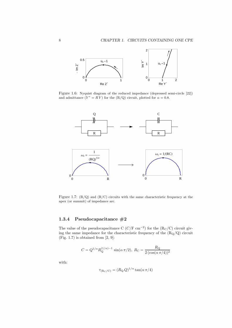
Figure 1.6: Nyquist diagram of the reduced impedance (depressed semi-circle [22])and admittance (Y ∗ = R Y ) for the (R/Q) circuit, plotted for α = 0.8.

R

Q

R

C

0 R0

Ωc=1

HRQL1Α

0 R0

Ωc= 1HRCL

Figure 1.7: (R/Q) and (R/C) circuits with the same characteristic frequency at theapex (or summit) of impedance arc.

1.3.4 Pseudocapacitance #2

The value of the pseudocapacitance C (C/F cm−2) for the (RC/C) circuit giv-ing the same impedance for the characteristic frequency of the (RQ/Q) circuit(Fig. 1.7) is obtained from [2, 9]:

C = Q1/αR(1/α)−1Q sin(α π/2), RC =

RQ

2 (cos(α π/4))2

with:

τ(RC/C) = (RQ Q)1/α tan(α π/4)

1.4. CIRCUIT (R/Q)+(R/Q)+ .. (VOIGT) 9

RQ

Q

RC

C

0 RC RQ0

Re Z

-Im

Z

Ωc =1

JRQ QN1Α

Figure 1.8: (RQ/Q) and (RC/C) circuits with the same impedance for the character-istic frequency of the (RQ/Q) circuit.

1.4 Circuit (R/Q)+(R/Q)+ .. (Voigt)

Z(ω) =

nRQ∑

i=1

Ri

1 + τi (i ω)αi; τi = Ri Qi

Re Z(ω) =

nRQ∑

i=1

Ri (1 + τi ωαi cαi)

1 + τ2i ω2 αi + 2 τi ωαi cαi)

Im Z(ω) = −

nRQ∑

i=1

Ri τi ωαi sαi

1 + τ2i ω2 αi + 2 τi ωαi cαi

1.5 Circuit (R1+(R2/Q2))

R1

R2

Q2

Figure 1.9: Circuit (R1+(R2/Q2)).


1.5.1 Impedance

Z(ω) = R1 +1

(i ω)α2 Q2 +1

R2

Z(ω) =(R1 + R2) (1 + (i ω)α2 τ2)

1 + (i ω)α2 τ1, τ1 = R2 Q2, τ2 =

R1 R2 Q2

R1 + R2


Z∗(u) =Z(u)

R1 + R2=

1 + T (i u)α2

1 + (i u)α2(1.1)

u = τ1/α2

1 ω, T = τ2/τ1 = R1/(R1 + R2) < 1

Re Z∗(u) =T cα uα2 + cα uα2 + Tu2α2 + 1

2 cα uα2 + u2α2 + 1

Im Z∗(u) = −(1 − T )uα2 sα

2 cα uα2 + u2α2 + 1

0 R1 R1+R2

0

Re Z

-Im

Z

Ωc=1

Τ11Α

1

Τ21Α

0 T 10

Re Z*

-Im

Z* uc= 1

1

T1Α

Figure 1.10: Nyquist diagrams of the impedance and reduced impedance for the(R1+(R2/Q2)) circuit.

1.6 Circuit (R1/(R2+Q2))

R2

R1

Q2

Figure 1.11: Circuit (R1/(R2+Q2)).

1.7. TRANSFORMATION FORMULAE BETWEEN(R+(R/Q)) AND (R/(R+Q))11

1.6.1 Impedance

Z(ω) =R1 (1 + τ2 (i ω)α2)

1 + τ1 (i ω)α2, τ1 = (R1 + R2)Q2, τ2 = R2 Q2

Re Z(ω) =R1

(

cos(

πα2

2

)

(τ1 + τ2)ωα2 + τ1τ2ω2α2 + 1

)

τ1

(

τ1ωα2 + 2 cos(

πα2

2

))

ωα2 + 1

Im Z(ω) = −ωα2 sin

(

πα2

2

)

R1 (τ1 − τ2)

τ1

(

τ1ωα2 + 2 cos(

πα2

2

))

ωα2 + 1


Z∗(u) =Z(u)

R1=

1 + T (i u)α2

1 + (i u)α2

u = τ1/α2

1 ω, T = τ2/τ1 = R2/(R1 + R2) < 1

cf. Eq. (1.1) and Fig. 1.10.

1.7 Transformation formulae between(R+(R/Q))and (R/(R+Q))

1.7.1 α21 = α22

R11

R21

Q21

R22

R12

Q22

Figure 1.12: The (R+(R/Q)) and (R/(R+Q)) circuits are non-distinguishable forα21 = α22 [1].

Transformations formulae (R+(R/Q)) → (R/(R+Q))

R12 = R11 + R21, R22 =R2

11

R21+ R11, Q22 =

Q21R221

(R11 + R21) 2

Transformations formulae (R/(R+Q))→(R+(R/Q))

Q21 =Q22 (R12 + R22)

2

R212

, R11 =R12R22

R12 + R22, R21 =

R212

R12 + R22

1.7.2 α21 6= α22

The (R+(R/Q)) and (R/(R+Q)) circuits (Fig. 1.12) are distinguishable forα21 6= α22


Chapter 2

Circuits made of two CPEs

2.1 Circuit (Q1+Q2)

Q1 Q2

Figure 2.1: Circuit (Q1+Q2).

2.1.1 α1 = α2 = α

Z(ω) =

(

1

Q1+

1

Q2

)

1

(i ω)α=

1

Q (i ω)α, Q =

Q1 Q2

Q1 + Q2

cf. § 1.1.

2.1.2 α1 6= α2

Impedance

Z(ω) =1

Q1 (i ω)α1+

1

Q2 (i ω)α2=

Q1 (i ω)α1 + Q2 (i ω)α2

Q1 Q2 (i ω)α1+α2

Re Z(ω) =cos(

πα1

2

)

ω−α1

Q1+

cos(

πα2

2

)

ω−α2

Q2

Im Z(ω) = −sin(

πα1

2

)

ω−α1

Q1−

sin(

πα2

2

)

ω−α2

Q2

|ZQ1| = |ZQ2

| ⇒ ω = ωc =

(

Q2

Q1

)1

α1−α2

13

14 CHAPTER 2. CIRCUITS MADE OF TWO CPES

• α1 < α2 (Figs. 2.2 and 2.3)

ω → 0 ⇒ Z(ω) ≈1

Q2 (i ω)α2, ω → ∞ ⇒ Z(ω) ≈

1

Q1 (i ω)α1

• α1 > α2

ω → 0 ⇒ Z(ω) ≈1

Q1 (i ω)α1, ω → ∞ ⇒ Z(ω) ≈

1

Q2 (i ω)α2

0 2000

200

Re ZW

-Im

ZW

1 4

1

4

logHRe ZWL

logH-

ImZWL

Figure 2.2: Nyquist and log Nyquist [8] diagrams of the impedance for the (Q1+Q2)circuit, plotted for Q1 = 10−2 F cm−2 sα1−1, Q2 = 10−2 F cm−2 sα2−1, α1 = 0.6, α2 =0.9 (α1 < α2). Dots: ωc = (Q2/Q1)

1/(α1−α2).

-5 5HQ2Q1L1HΑ1-Α2L

0

5

log ΩHrd s-1L

logÈZWÈ

- Α2

- Α1


-45

-90

log ΩHrd s-1L

ΦZ°

-Α1 Π2

-Α2 Π2

Figure 2.3: Bode diagrams of the impedance for the (Q1+Q2) circuit. Same valuesof parameters as in Fig. 2.2. α1 < α2.


Z∗(u) = Q1 ωα1

c Z(ω) =1

(i u)α1+

1

(i u)α2, u =

ω

ωc

2.1. CIRCUIT (Q1+Q2) 15

0 1 2 30

1

2

3

Re Z*

-Im

Z*

-2 0 2-2

0

2

log HRe Z*L

logH-

ImZ*L

Figure 2.4: Nyquist and log Nyquist [8] diagrams of the reduced impedance for the(Q1+Q2) circuit, plotted for α1 = 0.6, α2 = 0.9 (α1 < α2). Dots: uc = 1.

-3 30

-3

0

3

log u

logÈZ*È

- Α2

- Α1

-3 30

-45

-90

log u

ΦZ*°

-Α1 Π2

-Α2 Π2

Figure 2.5: Bode diagrams of the impedance for the (Q1+Q2) circuit. Same valuesof parameters as in Fig. 2.4. α1 < α2.


2.2 Circuit (Q1/Q2)

Q1

Q2

Figure 2.6: Circuit (Q1/Q2).

2.2.1 α1 = α2 = α

Z(ω) =1

(Q1 + Q2) (i ω)α=

1

Q (i ω)α, Q = Q1 + Q2

cf. § 1.1.

2.2.2 α1 6= α2

Impedance

Z(ω) =1

Q1 (i ω)α1 + Q2 (i ω)α2

Re Z(ω) =cos(

πα1

2

)

Q1ωα1 + cos

(

πα2

2

)

Q2ωα2

Q21ω

2α1 + Q22ω

2α2 + 2 cos(

12π (α1 − α2)

)

Q1Q2ωα1+α2

Im Z(ω) = −sin(

πα1

2

)

Q1ωα1 + sin

(

πα2

2

)

Q2ωα2

Q21ω

2α1 + Q22ω

2α2 + 2 cos(

12π (α1 − α2)

)

Q1Q2ωα1+α2

• α1 < α2 (Figs. 2.7 and 2.8)

ω → 0 ⇒ Z(ω) ≈1

Q1 (i ω)α1, ω → ∞ ⇒ Z(ω) ≈

1

Q2 (i ω)α2

• α1 > α2

ω → 0 ⇒ Z(ω) ≈1

Q2 (i ω)α2, ω → ∞ ⇒ Z(ω) ≈

1

Q1 (i ω)α1


Z∗(u) = Q1 ωα1

c Z(ω) =1

(i u)α1 + (i u)α2, u =

ω

ωc

2.2. CIRCUIT (Q1/Q2) 17

0 500

50

Re ZW

-Im

ZW

0 3

0

3

logHRe ZWL

logH-

ImZWL

Figure 2.7: Nyquist and log Nyquist [8] diagrams of the impedance for the (Q1/Q2)circuit plotted for Q1 = 10−2 F cm−2 sα1−1, Q2 = 10−2 F cm−2 sα2−1, α1 = 0.6, α2 =0.9 (α1 < α2). Dots: ωc = (Q2/Q1)

1/(α1−α2).


0

5

log ΩHrd s-1L

logÈZWÈ

- Α1

- Α2


-45

-90

log ΩHrd s-1L

ΦZ°

-Α1 Π2

-Α2 Π2

Figure 2.8: Bode diagrams of the impedance for the (Q1/Q2) circuit. Same values ofparameters as in Fig. 2.7. α1 < α2.

0 10

1

Re Z*

-Im

Z*

-2 0 2-2

0

2

log HRe Z*L

logH-

ImZ*L

Figure 2.9: Nyquist and log Nyquist [8] diagrams of the reduced impedance for the(Q1/Q2) circuit, plotted for α1 = 0.6, α2 = 0.9 (α1 < α2). Dots: uc = 1.


-3 30

-3

0

3

log u

logÈZ*È

- Α1

- Α2

-3 30

-45

-90

log u

ΦZ*°

-Α1 Π2

-Α2 Π2

Figure 2.10: Bode diagrams of the impedance for the (Q1/Q2) circuit. Same valuesof parameters as in Fig. 2.9. α1 < α2.

Chapter 3

Circuits made of one R andtwo CPEs

3.1 Circuit ((R1/Q1) + Q2)

Q2

Q1

R1

Figure 3.1: Circuit ((R1/Q1)+Q2).

3.1.1 α1 = α2 = α

Impedance

Z(ω) =1

1

R1+ Q1 (i ω)α

+1

Q2 (i ω)α

Z(ω) =1 + (i ω)α τ2

(i ω)α Q2 (1 + (i ω)α τ1), τ1 = R1 Q1, τ2 = (Q1 + Q2)R1, τ1 < τ2

Re Z(ω) = −cos(

πα2

) (

τ1τ2ω2α + 1

)

ω−α + cos(πα)τ1 + τ2

Q2(

τ1

(

τ1ωα + 2 cos(

πα2

))

ωα + 1)

Im Z(ω) = −sin(

πα2

) (

τ1τ2ω2α + 1

)

ω−α + sin(πα)τ1

Q2(

τ1

(

τ1ωα + 2 cos(

πα2

))

ωα + 1)

19

20 CHAPTER 3. CIRCUITS MADE OF ONE R AND TWO CPES

Reduced impedance

Z∗(u) =Z(u)

R1=

1

T − 1

1 + T (i u)α

(i u)α (1 + (i u)α)(3.1)

u = ω τ1/α, T = τ2/τ1 = 1 + Q2/Q1 > 1

Re Z∗(u) =u−α

(

(T + cos(απ))uα +(

Tu2α + 1)

cos(

απ2

))

(T − 1)(

2 cos(

απ2

)

uα + u2α + 1)

Im Z∗(u) = u−α

(

1

1 − T−

u2α

2 cos(

απ2

)

uα + u2α + 1

)

sin(απ

2

)

0 10

1

2

Re Z *

-Im

Z*

Figure 3.2: Nyquist diagram of the reduced impedance for the ((R1/Q1)+Q2) circuit(Fig. 3.1, Eq. (3.1)), plotted for T = 4, 9, 90 and α = 0.85. The line thickness increaseswith increasing T . Dots: reduced characteristic angular frequency uc1 = 1; circles:reduced characteristic angular frequency uc2 = 1/T 1/α (φuc1 = φuc2).

3.1.2 α1 6= α2

Impedance

Z(ω) =1

1

R1+ Q1 (i ω)α1

+1

Q2 (i ω)α2

Re Z(ω) =cos(

πα2

2

)

ω−α2

Q2+

R1

(

cos(

πα1

2

)

Q1R1ωα1 + 1

)

Q1R1

(

Q1R1ωα1 + 2 cos(

πα1

2

))

ωα1 + 1

Im Z(ω) = −sin(

πα1

2

)

Q1R21ω

α1

Q1R1

(

Q1R1ωα1 + 2 cos(

πα1

2

))

ωα1 + 1−

sin(

πα2

2

)

ω−α2

Q2

3.2. CIRCUIT ((R1 + Q1)/Q2) 21

R1

Q1

Q2

Figure 3.3: Circuit ((R1+Q2)/Q1).

3.2 Circuit ((R1 + Q1)/Q2)

3.2.1 α1 = α2 = α

Impedance

Z(ω) =1

(i ω)α Q1 +1

R1 +1

(i ω)α Q2

=1 + Q2 R1(i ω)α

(i ω)α (Q1 + Q2)

(

1 +(i ω)α Q1 Q2 R1

Q1 + Q2

)

Z(ω) =1 + τ2(i ω)α

(i ω)α (Q1 + Q2) (1 + (i ω)α τ1), τ1 =

Q1 Q2 R1

Q1 + Q2, τ2 = Q2 R1

Re Z(ω) =ω−α

(

cos(πα)ωα + τ2ωα + cos

(

πα2

) (

τ2ω2α + 1

))

(

2 cos(

πα2

)

ωα + ω2α + 1)

(Q1 + Q2) τ1

Im Z(ω) = −ω−α sin

(

πα2

) (

2 cos(

πα2

)

ωα + τ2ω2α + 1

)

(

2 cos(

πα2

)

ωα + ω2α + 1)

(Q1 + Q2) τ1

Reduced impedance

Z∗(u) =Z(u)

R1=

T − 1

T 2

1 + T (i u)α

(i u)α (1 + (i u)α)(3.2)

u = ω τ1/α, T = τ2/τ1 = 1 + Q2/Q1 > 1

Re Z∗(u) =(T − 1)u−α

(

(T + cos(απ))uα +(

Tu2α + 1)

cos(

απ2

))

T 2(

2 cos(

απ2

)

uα + u2α + 1)

Im Z∗(u) = −(T − 1)u−α

(

2 cos(

απ2

)

uα + Tu2α + 1)

sin(

απ2

)

T 2(

2 cos(

απ2

)

uα + u2α + 1)

3.2.2 α1 6= α2

Z(ω) =

1

(i ω)α2 Q2+ R1

(i ω)α1 Q1

(

1

(i ω)α1 Q1+

1

(i ω)α2 Q2+ R1

)

22 CHAPTER 3. CIRCUITS MADE OF ONE R AND TWO CPES

0 10

1

2

Re Z *

-Im

Z*

Figure 3.4: Nyquist diagram of the reduced impedance for the ((R1+Q1)/Q2) circuit(Fig. 3.3, Eq. (3.2)), plotted for T = 4, 9, 90 and α = 0.85. The line thickness increaseswith increasing T . Dots: reduced characteristic angular frequency uc1 = 1; circles:reduced characteristic angular frequency uc2 = 1/T 1/α (φuc1 = φuc2).

Z(ω) =1 + τ (i ω)

α2

(i ω)α1 Q1 + (i ω)α2 Q2 + τ (i ω)α1+α2 Q1

, τ = R1 Q2

Re Z(ω) =(

ωα1 cα1

(

1 + τ2 ω2 α2 + 2 τ ωα2 cα2

)

Q1 + ωα2 (τ ωα2 + cα2) Q2

)

/(

ω2 α1(

1 + τ2 ω2 α2 + 2 τ ωα2 cα2

)

Q12 + 2 ωα1+α2 (τ ωα2 cα1 + cα1mα2) Q1 Q2 + ω2 α2 Q2

2)

cα1mα2 = cos

(

π (α1 − α2)

2

)

Im Z(ω) =(

−ωα1(

1 + τ2 ω2 α2 + 2 τ ωα2 cα2

)

Q1 sα1 − ωα2 Q2 sα2

)

/(

ω2 α1(

1 + τ2 ω2 α2 + 2 τ ωα2 α2)

Q12 + 2 ωα1+α2 (τ ωα2 cα1 + cα1mα2) Q1 Q2 + ω2 α2 Q2

2)

Chapter 4

Circuits made of two Rsand two CPEs

4.1 Circuit ((R1/Q1)+(R2/Q2))

R1

Q1

R2

Q2

Figure 4.1: Circuit ((R1/Q1)+(R2/Q2)).

Z(ω) =1

(i ω)α1 Q1 +1

R1

+1

(i ω)α2 Q2 +1

R2

Z(ω) =R1

1 + (i ω)α1 τ1

+R2

1 + (iω)α2 τ2

, τ1 = R1 Q1 , τ2 = R2 Q2

Z(ω) =R1 + R2 + (i ω)

α1 R2 τ1 + (i ω)α2 R1 τ2

(1 + (i ω)α1 τ1) (1 + (i ω)

α2 τ2)

Re Z(ω) =R1 (1 + ωα1 cα1 τ1)

1 + ωα1 τ1 (2 cα1 + ωα1 τ1)+

R2 (1 + ωα2 cα2 τ2)

1 + ωα2 τ2 (2 cα2 + ωα2 τ2)

Im Z(ω) = −ωα1 R1 sα1 τ1

1 + ωα1 τ1 (2 cα1 + ωα1 τ1)−

ωα2 R2 sα2 τ2

1 + ωα2 τ2 (2 cα2 + ωα2 τ2)

23

24 CHAPTER 4. CIRCUITS MADE OF TWO RS AND TWO CPES

0 0.5 10

0.3

Re Z *

-Im

Z* uc1 uc2

Figure 4.2: Nyquist diagrams of the reduced impedance for the ((R1/Q1)+(R2/Q2))circuit (Fig. 4.1). R1 = R2, α1 = α2, Q2 ≫ Q1.

0 0.5 10

0.5

Re Z *

-Im

Z*

uc1 = uc2

0 0.5 10

0.5

Re Z *

-Im

Z*

uc1 = uc2

- Π4 Π4

Figure 4.3: Unusual Nyquist diagrams of the reduced impedance for the((R1/Q1)+(R2/Q2)) circuit (Fig. 4.1). R1 = R2, Q2 = Q1, α1 = 1. Left: α2 = 0.3,right: α2 = 0.5.

4.2 Circuit ((R1+(R2/Q2))/Q1)

Z(ω) =1

(i ω)α1 Q1 +

1

R1 +1

(i ω)α2 Q2 +

1

R2

Z(ω) =R1 + R2 + (i ω)

α2 Q2 R1 R2

1 + (i ω)α1 Q1 (R1 + R2) + (i ω)α2 Q2 R2 + (i ω)α1+α2 Q1 Q2 R1 R2

R1

Q1

Q2

R2

Figure 4.4: Circuit ((R1+(R2/Q2))/Q1).

4.3. CIRCUIT ((Q1+(R2/Q2))/R1) 25

Re Z(ω) =(

R1 + R2 + ω2 α2 Q22 R1 (1 + ωα1 Cα1 Q1 R1) R2

2+

ωα1 Cα1 Q1 (R1 + R2)2

+ ωα2 Cα2 Q2 R2 (R2 + 2 R1 (1 + ωα1 Cα1 Q1 (R1 + R2))))

/(

1 + ω2 α2 Q22 (1 + ωα1 Q1 R1 (2 Cα1 + ωα1 Q1 R1)) R2

2+

ωα1 Q1 (R1 + R2) (2 Cα1 + ωα1 Q1 (R1 + R2)) + 2 ωα2 Q2 R2

× (Cα2 + ωα1 Q1 (Cα1mα2 R2 + Cα2 R1 (2 Cα1 + ωα1 Q1 (R1 + R2)))))

cα1mα2 = cos

(

π (α1 − α2)

2

)

Im Z(ω) =(

ωα1 Q1

(

−ω2 α2 Q22 R1

2 R22 − 2 ωα2 Cα2 Q2 R1 R2 (R1 + R2)−

(R1 + R2)2)

Sα1 − ωα2 Q2 R22 Sα2

)

/(

1 + ω2 α2 Q22 (1 + ωα1 Q1 R1 (2 Cα1 + ωα1 Q1 R1)) R2

2+

ωα1 Q1 (R1 + R2) (2 Cα1 + ωα1 Q1 (R1 + R2)) + 2 ωα2 Q2 R2

× (Cα2 + ωα1 Q1 (Cα1mα2 R2 + Cα2 R1 (2 Cα1 + ωα1 Q1 (R1 + R2)))))

4.3 Circuit ((Q1+(R2/Q2))/R1)

Q1

R1

Q2

R2

Figure 4.5: Circuit ((Q1+(R2/Q2))/R1).

Z(ω) =1

1

R1+

11

(i ω)α1 Q1

+1

(i ω)α2 Q2 +

1

R2

Z(ω) =R1 (1 + (i ω)α1 Q1 R2 + (i ω)α2 Q2 R2)

1 + (i ω)α1 Q1 (R1 + R2) + (i ω)

α2 Q2 R2 + (i ω)α1+α2 Q1 Q2 R1 R2


Re Z(ω) =(

R1

(

1 + ωα2 Q2 R2 (2 Cα2 + ωα2 Q2 R2) + ω2 α1 Q12 R2

× (R2 + R1 (1 + ωα2 Cα2 Q2 R2)) + ωα1 Q1 (2 R2 (Cα1 + ωα2 Cα1mα2 Q2 R2)+

Cα1 R1 (1 + ωα2 Q2 R2 (2 Cα2 + ωα2 Q2 R2))))) /(

1 + ω2 α2 Q22 (1 + ωα1 Q1 R1 (2 Cα1 + ωα1 Q1 R1)) R2

2+

ωα1 Q1 (R1 + R2) (2 Cα1 + ωα1 Q1 (R1 + R2))+

2 ωα2 Q2 R2 (Cα2 + ωα1 Q1 (Cα1mα2 R2 + Cα2 R1 (2 Cα1 + ωα1 Q1 (R1 + R2)))))

Im Z(ω) = −ωα1 Q1 R22 (Sα1 + ωα2 Q2 R2 ((2 Cα2 + ωα2 Q2 R2) Sα1 + ωα1 Q1 R2 Sα2)) /

(

1 + ω2 α2 Q22 (1 + ωα1 Q1 R1 (2 Cα1 + ωα1 Q1 R1)) R2

2+

ωα1 Q1 (R1 + R2) (2 Cα1 + ωα1 Q1 (R1 + R2))+

2 ωα2 Q2 R2 (Cα2 + ωα1 Q1 (Cα1mα2 R2 + Cα2 R1 (2 Cα1 + ωα1 Q1 (R1 + R2)))))

Z(ω) =R1 (1 + τ1 (i ω)α1 + τ2 (i ω)α2)

1 + (1 + R1/R2) τ1 (iω)α1 + τ2 (i ω)

α2 + τ1 τ2 (R1/R2) (i ω)α1+α2

τ1 = Q1 R2 , τ2 = Q2 R2

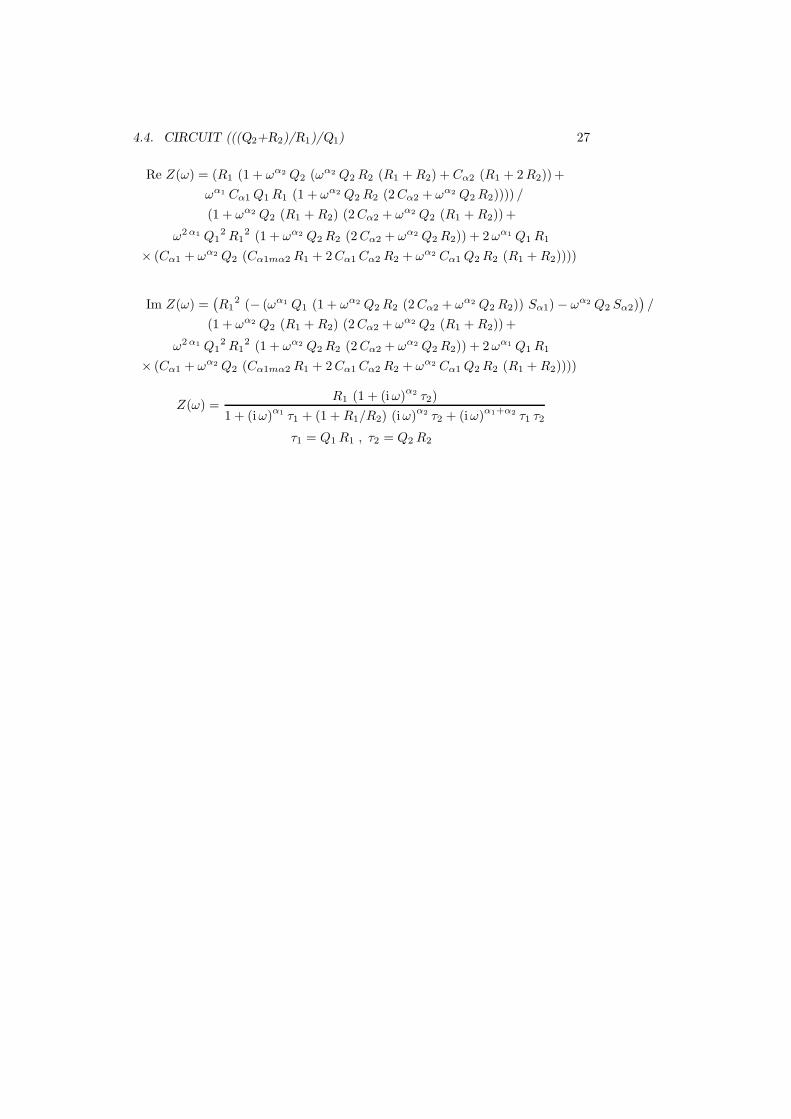
4.4 Circuit (((Q2+R2)/R1)/Q1)

Q2

R2

R1

Q1

Figure 4.6: Circuit (((Q2+R2)/R1)/Q1).

Z(ω) =1

(i ω)α1 Q1 +1

R1+

11

(i ω)α2 Q2

+ R2

Z(ω) =R1 (1 + (iω)α2 Q2 R2)

1 + (i ω)α1 Q1 R1 + (i ω)

α2 Q2 R1 + (i ω)α2 Q2 R2 + (i ω)

α1+α2 Q1 Q2 R1 R2

4.4. CIRCUIT (((Q2+R2)/R1)/Q1) 27

Re Z(ω) = (R1 (1 + ωα2 Q2 (ωα2 Q2 R2 (R1 + R2) + Cα2 (R1 + 2 R2))+

ωα1 Cα1 Q1 R1 (1 + ωα2 Q2 R2 (2 Cα2 + ωα2 Q2 R2)))) /

(1 + ωα2 Q2 (R1 + R2) (2 Cα2 + ωα2 Q2 (R1 + R2)) +

ω2 α1 Q12 R1

2 (1 + ωα2 Q2 R2 (2 Cα2 + ωα2 Q2 R2)) + 2 ωα1 Q1 R1

× (Cα1 + ωα2 Q2 (Cα1mα2 R1 + 2 Cα1 Cα2 R2 + ωα2 Cα1 Q2 R2 (R1 + R2))))

Im Z(ω) =(

R12 (− (ωα1 Q1 (1 + ωα2 Q2 R2 (2 Cα2 + ωα2 Q2 R2)) Sα1) − ωα2 Q2 Sα2)

)

/

(1 + ωα2 Q2 (R1 + R2) (2 Cα2 + ωα2 Q2 (R1 + R2)) +

ω2 α1 Q12 R1

2 (1 + ωα2 Q2 R2 (2 Cα2 + ωα2 Q2 R2)) + 2 ωα1 Q1 R1

× (Cα1 + ωα2 Q2 (Cα1mα2 R1 + 2 Cα1 Cα2 R2 + ωα2 Cα1 Q2 R2 (R1 + R2))))

Z(ω) =R1 (1 + (i ω)

α2 τ2)

1 + (i ω)α1 τ1 + (1 + R1/R2) (i ω)α2 τ2 + (i ω)α1+α2 τ1 τ2

τ1 = Q1 R1 , τ2 = Q2 R2


Appendix A

Symbols for CPE

29

30 APPENDIX A. SYMBOLS FOR CPE

A B CCPE

DE

F

G HQ

I

J K L

M N O

ÙÙP Q R

S T

Figure A.1: Some CPE symbols, taken from A: [13], B: [19], C: [23], D: [5], E: [10],F: [17], G: [18], H: [21], I: [12], J: [15], K: [20], L: [2, 9], M: [11], N: [3, 4], O: [14], P:[24], Q, R [25], S [7], T [16].

Bibliography

[1] Berthier, F., Diard, J.-P., and Montella, C. Distinguishability ofequivalent circuits containing CPEs. I. Theoretical part. J. Electroanal.

Chem. 510 (2001), 1–11.

[2] Boillot, M. Validation experimentale d’outil de modelisation d’une pile

a combustible de type PEM. PhD thesis, INPL, Nancy, Oct. 2005.

[3] Bommersbach, P., Alemany-Dumont, C., Millet, J., and Nor-

mand, B. Formation and behaviour study of an environment-friendlycorrosion inhibitor by electrochemical methods. Electrochim. Acta 51, 6(2005), 1076 – 1084.

[4] Bommersbach, P., Alemany-Dumont, C., Millet, J.-P., and Nor-

mand, B. Hydrodynamic effect on the behaviour of a corrosion inhibitorfilm: Characterization by electrochemical impedance spectroscopy. Elec-

trochimica Acta 51, 19 (2006), 4011 – 4018.

[5] Brug, G. J., van den Eeden, A. L. G., Sluyters-Rehbach, M., and

Sluyters, J. H. The analysis of electrode impedance complicated by thepresence of a constant phase element. J. Electroanal. Chem. 176 (1984),275–295.

[6] Chabli, A., Diaco, T., and Diard, J.-P. Determination de lasequence de ponderation d’une pile leclanche a l’aide d’une methoded’intercorrelation. J. Applied Electrochem. 11 (1981), 661.

[7] Ding, S.-J., Chang, B.-W., Wu, C.-C., Lai, M.-F., and Chang, H.-

C. Impedance spectral studies of self-assembly of alkanethiols with differentchain lengths using different immobilization strategies on au electrodes.Analytica Chimica Acta 554 (2005), 43 – 51.

[8] Fournier, J., Wrona, P. K., Lasia, A., Lacasse, R., Lalancette,

J.-M., Menard, H., and Brossard, L. J. Electrochem. Soc. 139 (1992),2372.

[9] Franck-Lacaze, L., Bonnet, C., Besse, S., and Lapicque, F. Effectof ozone on the performance of a polymer electrolyte membrane fuel cell.Fuel Cells 09 (2009), 562–569.

[10] Han, D. G., and Choi, G. M. Computer simulation of the electricalconductivity of composites: the effect of geometrical arrangement. Solid

State Ionics 106 (1998), 71–87.

31

32 BIBLIOGRAPHY

[11] Hernando, J., Lud, S. Q., Bruno, P., Gruen, D. M., Stutz-

mann, M., and Garrido, J. A. Electrochemical impedance spectroscopyof oxidized and hydrogen-terminated nitrogen-induced conductive ultra-nanocristalline diamond. Electrochim. Acta 54 (2009), 1909–1915.

[12] Holzapfel, M., Martinent, A., Alloin, F., B. Le Gorrec, Yazami,

R., and Montella, C. First lithiation and charge/discharge cyclesof graphite materials, investigated by electrochemical impedance spec-troscopy. J. Electroanal. Chem. 546 (2003), 41–50.

[13] Jansen, R., and Beck, F. Electrochim. Acta 39 (1994), 921.

[14] Jonscher, A. K., and Bari, M. A. Admittance spectroscopy of sealedprimary batteries. J. Electrochem. Soc. 135 (1988), 1618–1625.

[15] Kulova, T. L., Skundin, A. M., Pleskov, Y. V., Terukov, E. I.,

and Kon’kov, O. I. Lithium insertion into amorphous silicon thin-filmelectrode. J. Electroanal. Chem. 600 (2007), 217–225.

[16] Laes, K., Bereznev, S., Land, R., Tverjanovich, A., Volobujeva,

O., Traksmaa, R., Raadik, T., and Opik, A. The impedance spec-troscopy of photoabsorber films prepared by high vacuum evaporation tech-nique. Energy Procedia 2, 1 (2010), 119 – 131.

[17] Matthew-Esteban, J., and Orazem, M. E. On the application of theKramers-Kronig relations to evaluate the consistency of electrochemicalimpedance data. J. Electrochem. Soc. 138 (1991), 67–76.

[18] Messaoudi, B., Joiret, S., Keddam, M., and Takenouti, H. Anodicbehaviour of manganese in alkaline medium. Electrochim. Acta 46 (2001),2487–2498.

[19] Orazem, M. E., Shukla, P. S., and Membrino, M. A. Extension of themeasurement model approach for deconvolution of underlying distributionsfor impedance measurements. Electrochim. Acta 47 (2002), 2027–2034.

[20] Quintin, M., Devos, O., Delville, M. H., and Campet, G. Studyof the lithium insertion-deinsertion mechanism in nanocrystalline γ-Fe2O3

electrodes by means of electrochemical impedance spectroscopy. Elec-

trochim. Acta 51 (2006), 6426–6434.

[21] Seki, S., Kobayashi, Y., Miyashiro, H., Yamanaka, A., Mita, Y.,

and Iwahori, T. Degradation mechanism analysis of all solid-state lithiumpolymer rechargeable batteries. In IMBL 12 Meeting (2004), The Electro-chemical Society. Abs. 386.

[22] Sluyters-Rehbach, M. Impedance of electrochemical systems: termi-nology, nomenclature and representation-part I: cells with metal electrodesand liquid solution (IUPAC Recommendations 1994). Pure & Appl. Chem.

66 (1994), 1831–1891.

[23] Tomczyk, P., and Mosialek, M. Investigation of the oxygen electrodereaction in basic molten carbonates using electrochemical impedance spec-troscopy. Electrochim. Acta 46 (2001), 3023–3032.

BIBLIOGRAPHY 33

[24] VanderNoot, T. J., and Abrahams, I. The use of genetic algorithmsin the non-linear regression of immittance data. J. Electroanal. Chem. 448

(1998), 17–23.

[25] Yang, B. Y., and Kim, K. Y. The oxidation behavior of Ni-50%Coalloy electrode in molten Li + K carbonate eutectic. Electrochim. Acta 44

(1999), 2227–2234.

[26] Zoltowski, P. J. Electroanal. Chem. 443 (1998), 149.

Documents

Handbook of Electrochemical Impedance Spectroscopy ELECTRICAL CIRCUITS CONTAINING