Embed Size (px)
Citation preview

Technical Report No. 1Document No. P-7376-TRI
Contract No. NAS 5-25341
June 1979
Prepared for
NASA Goddard Space Flight Center
Greenbelt, Maryland 20771
_N8_ 3ol i_}I_I|I11|II1111111111I11
_'. - _.
_'2--.__- ...... ": _--= .7.
(UASA-CB-lb5002}- I.illal;Booz-l_oa TBE ; 1182-12301ESTZ_ATZON OF BZCROB&V£ PIOPAGATIOB E_CTS: ._ -=. _..._:
LINK CALCULATIONS FOR £&R_H-SPACE PAT_S ._ ,_=/"
(PATH LOSS AND NOIS_ _STIZATIOB) I"_, .........
{Envi_oa.ental Hesearch and T_¢hnology# _.___.G3/32__ ..08_29i--
Handbook for theestimation of microwave
propagation effects--link calculations for
earth-space paths
i
Ji
,/
(.Path .Loss andNoxse Estxmatmn)
Robert K. Crane
David W. Blood
ENVIRONMENTAL RESEARCH &TECHNOLOGY, INC. - -CONCORD. MA ° LOS ANGELES - ATLANTA • PITTSBURGHFORT COLLINS. CO • BILLINGS, MT • HOUSTON • CHICAGO
._-7-
https://ntrs.nasa.gov/search.jsp?R=19820004428 2018-07-19T00:05:20+00:00Z


4. Title ar_l Subtitle 5.
Handbook for the Estimation of Microwave Propagation Effects -
Link Calculations for Earth-Space Paths {Path Loss and 8.'Noise Estimation)
ii m|
7. Author(s) 8.
Dr. Robert K. Crane and David W. Blood
10.
9. Pmfforrning Organization Natal and Addr=m
Environmental Research _ Technology, Inc. i1'.696 Virginia Road
Concord, Massachusetts 01742
13.
12. SDomoring Agency Name and Ac_nmNASA Goddard Space Flight Center
Greenbelt, Maryland 20771 14.
Technical Officer: Dr. Louis J. Ippolito
15. Supplementary Notes
&=June 1979
Performing Orpniz_ion Code
Technical Report No. I, ,m
Pl_orvning Orgenization Report No.
P-7376-TRJ
Work Unit No. '
m
Contract or Grant No.
NAS 5-25341
Ty_ of Report and I_lriod cover_l
Technical ReportSeot. 1978 to HaY 1979
Sl_nsorin 9 Agency Code
The authors gratefully acknowledge the helpful consultations of Dr. L. Ippolito
of NASA/GSFC during the period of reporting.
... , m,
16. Absl_
This report provides the path loss and noise estimation procedures as the basic input
to systems design for earth-to-space microwave links operating at frequencies from I to
300 GHz. Topics covered include gaseous absorption, attenuation by rain, scintillation,
low elevation angle effects, radome attenuation, diversity schemes, noise emission by
atmospheric gases, emission by rain and antenna contributions.
These sections are part of a handbook preparation project entitled "Handbook for the
Estimation of Microwave Propagation Effects," to include point-to-point microwave and
remote sensing systems design.
The models presented provide step-by-step procedures useful to system engineers in
system design, evaluation and frequency management.
17. K,y. wo,_ lS._W_ by Aum=,(,| )microwave vropagatlonCommunication Links
Earth-space Satellite Paths
Atmospheric Absorption
Rain Attenuation
Millimeter Waves
Unlimited
19. St¢.urity O_sif. Iof this rel=ort) 20. _rity Clmmif. [of this ;_ie}¢
Unclassified Unclassified
"For tile by the C1em-ingh_um fly Fedeflt Scientific and Vertical Information
Slm'ingfietcl. Virtlin_ 22151
21. No. of Pages
86i
22.


TABLE OF CONTENTS
Page
l,
2.
INTRODUCTION
PATH LOSS ESTIb_TION
2.1 Gaseous Absorption
2.1.1 Hodel
2.1.2 Procedure
2.1.3 Comparison with Experiment
2.2 Attenuation by Rain
2.2.1 Model
2.2.2 Procedure
2.2.3 Comparison with Experiment
2.3 Scintillation
2.5.1 Ionospheric Scintillation
2.5.2 Tropospheric Scintillation
2.5.5 Procedure
2.4 Low Elevation Angle Effects
2.4.1 Atmospheric Hultipath
2.4.2 Spreading Loss
2.4.5 Procedure
2.5 Rado_Attenuation
2.5.1 Dry Conditions
2.5.2 Wet Conditions
2.6 Diversity Schemes
2.6.1 Earth Terminal Site-Diversity
2.6.2 Satellite TerminalTechniques
2.7 Link Calculation
3. RECEIVER NOISE
3.1 Emission by Atmospheric Gases
3.2 Emission by Rain
3.3 Antenna Contributions
CONCLUSION
REFERENCES
EPrecedingpageblanki
iii
3
3
3
11
11
15
15
29
31
36
39
40
48
52
52
54
57
58
58
58
58
59
64
65
67
67
7O
75
76
77
-,...-


E_VI_II_NMF__NT_. RESEAFIC_ & TEC2-1NOLOGY INC
LIST OF ILLUSTRATIONS
Figure
I.
,
B
D
,
6a,b.
,
Be
,
lO.
Ii.
12a,b.
13.
Specific attenuation due to gaseous constituents
and precipitation for transmission within the
atmosphere [CCIR, 1977]
Theoretical one-way zenith attenuation from specified
height to top of the atmosphere for a moderately
humid atmosphere (Po = 7.5 g/m 3 at the surface)
Total zenith attenuation (dB) and deviation aboutthe all season and location mean (dB) for a one-way
path through the atmosphere from the surface
Coefficients a, b and c for equation 1 to compute
the total zenith attenuation (T90) knowing thesurface conditions
Illustration of oblique path attenuation through the
atmosphere compared with the zenith model value (M)
Global map of (Po) average absolute humidity (g/m5)
at the surface [Bean and Dutton, 1966] for February
and August
Comparison of humidity dependence of zenith attenua-tion computed (equation I) with measured values at22.235 GHz
Global rain rate climate regions for the continental
areas.
Global rain rate climate regions including the ocean
areas
Rain rate climate regions for the Continental United
States showing the subdivision of Region D
Rain rate climate regions for Europe.
Point rain rate distributions as a function of per-
cent of year exceeded - (a) Climate Regions A to H,
(b) Climate Regions D divided into three subregions
{D2 = D above)
Latitude dependence of the rain layer O°C isotherm
height (Ho) as a function of probability of occur-rence
i Precedingpageblank ...............i !
Page
4
5
12
13
14
17
18
19
20
21
24
V

• u
LIST OF ILLUSTRATIONS (cont)
Figure
14.
15.
16.
17.
18.
19.
20.
21.
24.
25.
26.
27.
28.
Hultiplier (_) in the power law relationship
between specific attenuation and frequency
F_ponent [B) in the power law relationship
between specific attenuation and frequency
Comparison of CTS attenuation observations at
11.7 GHz [after Ippolito) with model estimates
Comparison of observations (Figure 16) as percentdeviation from the model estimate
Comparison of observations as percent deviationfrom the model estimate for seven locations and
three frequencies
Elevation angle dependence of 11.8 GHz suntracker
observations at Klang, Halaysia [Climate Region H;after Kinase and Kinpara) compared with model
estimate
Comparison of point-to-point observations at five
frequencies on a 20-km path with model estimates
RHS fluctuations in elevation angle for a full year
period
Hedian RMS fluctuations in elevation angle by season
PJ4S fluctuations in log power (dB) for a fulI Tear
period
RMS fluctuations in log power at X-band and UHF,
29-30 April 1975
Comparison of tropospheric scintillation model with
Haystack [7.3 GHz) and Millstone [0.4 GHz) observa-
tions
Comparison of model predictions with observations
at 4 and 6 GHz [after Yokoi)
Comparison of model predictions (amplitude variance)
with ATS-6 observations at 2, 20 and 30 GHzJ
Hodel predictions of RMS fluctuations for an antennadiameter o£ I0 meters
Page
26
27
32
33
35
37
38
41
41
44
44
47
49
5O
S1
vi
LIST OF ILLUSTRATIONS (cont)
Figure
29a,b,c,d.
30.
31.
32.
37.
38.
39.
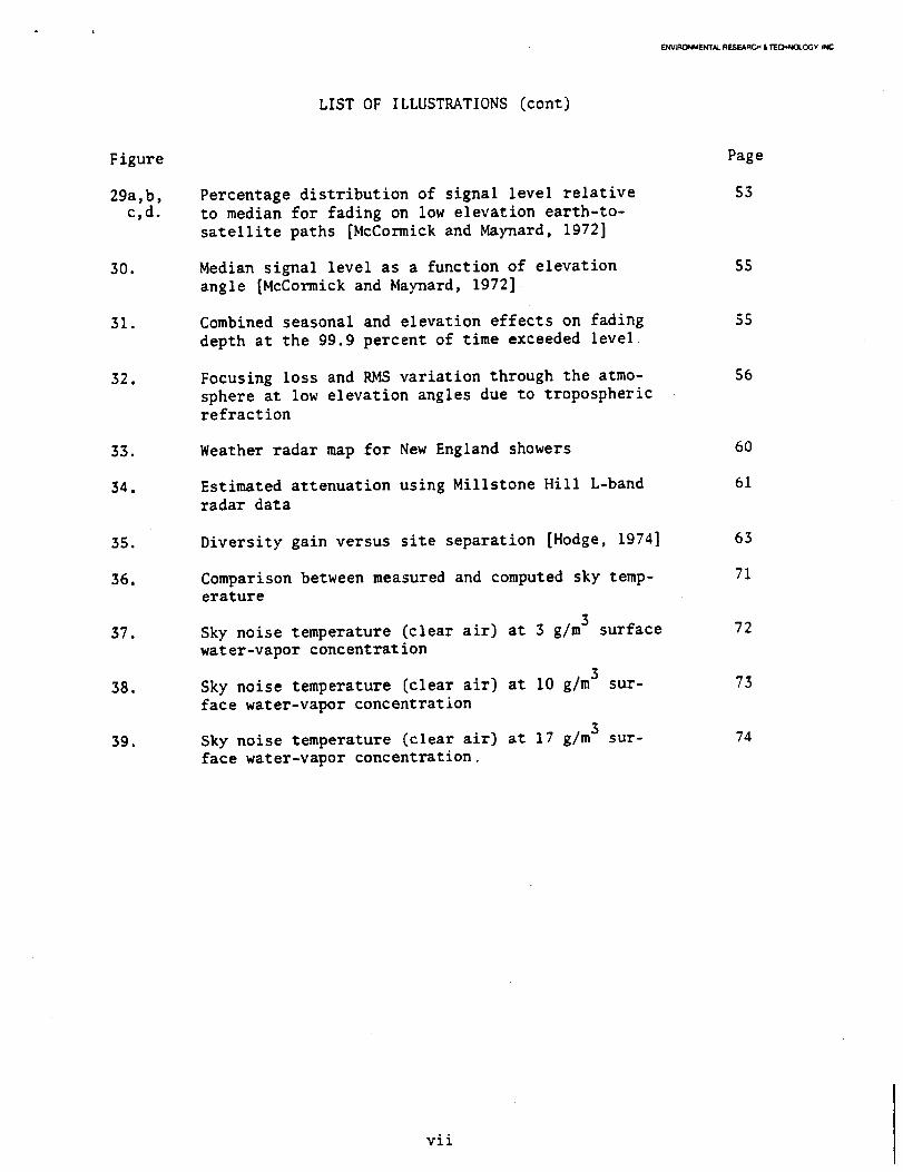
Percentage distribution of signal level relative
to median for fading on low elevation earth-to-
satellite paths [McCormick and Maynard, 1972]
Median signal level as a function of elevationangle [McCormick and Maynard, 1972].
Combined seasonal and elevation effects on fading
depth at the 99.9 percent of time exceeded level
Focusing loss and RMS variation through the atmo-
sphere at low elevation angles due to troposphericrefraction
Weather radar map for New England showers
Estimated attenuation using Millstone Hill L-band
radar data
Diversity gain versus site separation [Hodge, 1974]
Comparison between measured and computed sky temp-erature
Sky noise temperature (clear air) at 3 g/m 3 surface
water-vapor concentration
Sky noise temperature (clear air) at i0 g/m 3 sur-
face water-vapor concentration
Sky noise temperature (clear air) at 17 g/m 3 sur-
face water-vapor concentration.
Page
53
$5
55
56
60
61
63
71
72
73
74
vii


_W_N_na_A& _SaARO_ a7E_q_O_C_V _NC
LIST OF TABLES
Table
1.
2.
o
Coefficients for Computing Total Zenith Attenuation (dB)
Point Rain Rate (Rp) Distribution Values (mm/hr) versusPercent of Year Ramn Rate is Exceeded
Parameters for Computing Specific Attenuation:a = aR _ (dB/km)
P
Page
9
22
28
i Precedingpageblanki
ix


I. INTRODUCTION
As satellite and earth relay communication services continue to
expand in volume of usage, increased information bandwidth requirements,
and new applications, a consistent demand will be toward the use of
higher frequencies where permissible. The inuninent use of millimeter
wavebands [above 50 GHz) has prompted theoretical and experimental
studies of the limitations imposed by the atmosphere on line-of-sight
relay and earth-to-space [both up- and down-link) propagation paths. The
studies have shown that limitations arise mainly from signal attenuation
(absorption and scattering by the medium), noise emission (natural), or
interference (man-made) produced in part or wholly by propagation pheno-
mena. One of the principle causes of both attenuation, noise and poten-
tial interference is that caused by rain or hydrometeors. Although the
physics of scattering by hydrometeors is well in hand [Crane, 1971),
several different methodologies have developed to attempt to treat this
particular phenomenon, having a totally statistical occurrence behavior
as opposed to gaseous absorption and emission by the atmosphere which is
continuously present with only a statistical variation about the mean.
Attenuation caused by rain as well as the gaseous contribution increases
significantly to many tens of decibels at the higher frequencies deeper
into the millimeter wavebands.
It has therefore become imperative to have a consistent single
mode( available for a standard of co,Tparison for other models when deal-
ing with_$ain attenuation_r problems in System design and e____xperimentation
at the higher frequencies; .....This reppr! 9f_f_E.such a model a_. a proposed
standard technique. The latest refinements to the Global Rain Prgd_c!ionL
Model are incorporated in this handbook:. The basic model (with fewer
refinements) has previously been submitted for inclusion by the CCIR
(CCIR, 1978a) as a handbook tool for general application. With a size-
able amount of measurement data from satellite links operating at fre-
quencies up to 30 GHz now becoming available, the model can be easily
evaluated beyond that accomplished at present. The model is also amenable
to further refinements and updates as these data comparisons are made
and additional higher frequency data become available. Cases of model
usage and co,_arisons will be of extreme value, if fed back, to provide
the basis of information on which these further refinements may be made.

The frequency range treated in this report is from 1 to 300 GHz
(30 cm to 1 am wavelengths). The gaseous attenuation model spans this
range although caution should be exercised in its use at frequencies
above 200 GHz due to theoretical uncertainties in the water vapor model.
The rain model presented only covers the 1 to I00 GHz (30 cm to 3 mm
wavelength ) portion of the frequency range, although use at higher
frequencies is possible given adequate relationships between specific
attenuation and rain rate.
This report provides the path loss and noise estimation procedures
as the basic input to system design for earth-to-space link calculations.
These sections are part of a handbook preparation project for a complete
manual entitled "Handbook for the Estimation of Microwave Propagation
Effects." The handbook is designed to be used on three different levels,
(I) for step-by-step system design, (2) as a source book for communication
system evaluation and frequency management, and (3) for an up-to-date
survey of microwave propagation physics. This section on link calculations
for earth-space-paths defines the propagation models used for system
parameter estimati£n_and compares m0#el predictions with observations.
The propagation phenomena are only described in sufficient detail to be
useful in system evaluation and frequency management. Other sections of
the handbook provide a survey of the propagation physics, link calcula-
tions for ground-to_g[0und paths, and remote sensing system design. A
goal for the complete project is to provide a treatment of available
microwave data in a consistent manner with step-by-step procedures for
system design, curves, and computer adaptable algorithms to simplify
parameter estimation for the user.

ENVI_qQNMENTAL RE_C,_ &I"E ;HNOLO(3Y 1_4::
2. PATH LOSS ESTIMATION
2.1 Gaseous Absorption
Of the phenomena affecting earth-to-space propagation paths at micro-
wave frequencies, those due to gaseous absorption and rain are of prime
importance in system planning. The first of these, signal strength atten-
uation due to atmospheric absorption, is of fundamental concern in system
frequency selection, design and operation due to the strong frequency
dependence produced by molecular absorption lines at frequencies above
20 GHz. Atmospheric absorption must be dealt with continuously, whereas
the attenuation due to rain, clouds and fog, etc. must be treated statis-
tically on a percent of time basis. The gaseous specific attenuation
(dB/km) is predictable for a given set of layer parameters, e.g. sea
level pressure, temperature and humidity. Figure 1 (CCIR, 1977) shows
the absorption characteristics as a function of frequency for the spectrum
from i GHz through RF, I.R. and optical frequencies. Here the attenua-
tion (per unit distance) contrfbution of the gaseous constituents of the
medium are compared with those due to rain, at different rainfall rates,
and also due to fog. Though the overall attenuation characteristics are
very complex, the discussion in this report is limited to wavelengths
greater than one millimeter (frequencies below 300 GHz) where only four
of the absorption bands are of concern.
2.1.1 Model
Molecular absorption experienced on a path operating at centimeter
or millimeter wavelengths is due primarily to the atmospheric water vapor
and oxygen content (Waters, ]976). The absorption bands are centered at
frequencies of 22.2 GHz (H20), 60 GHz (O2), 118.8 GHz (O2), and 183 GHz
(H20). The lower three of these bands are depicted in Figure 2 which
presents the integrated zenith attenuation from 1 to 160 GHz. The total
one-way attenuation is shown from different starting heights to the top
of the atmosphere. The curves were computed (Crane, 1971) for temperate
latitudes* and moderate absolute humidity conditions (7.5 g/m3 at the
surface).
*U.S. Standard Atmosphere, July, 45°N.

4

ENVIR(_I_aF.NTAL RESEARCH • TEC;-tN(_I.OGY fl_C
I000 -
I00 -
I0-
I--< I
I-
Z1,1N
IUJZ0
/
_" .010p.
.001
STARTING HEIGHTS:
O
4
8
12
16
02
MINIMUM " I tVALUES FOR.
RANGE OFVALUES
0 2
.0001
Figure 2
• • = , , • , | I i a _ .... I
I0 IO0FREQUENCY (GHz}
Theoretical one-way zenith aCtenuation £ro= speci£iedheight to top o£ the atmosphere for a moderately
humid atmosphere (Po = 7. S g/m 3 a¢ the sur£ace)

The mean zenith attenuation and standard deviation of attenuation
for calculations made using a 220 profile sample of atmospheric condi-
tions spanning all seasons and geographical locations [Crane, 1976], is
presented in Figure 5. These results show, for example, that at frequen-
cies between 30 and 35 GHz, the variability of water vapor and temperature
produces less than a .14 dB [la) uncertainty in the zenith signal strength
for a path from. the surface to space. For oblique paths through the
a_mosphere, the attenuation as a function of elevation angle is given by
the zenith attenuation multiplied by the cosecant of the elevation angle.
The cosecant law does not hold for elevation angles less than about 6"
due to earth curvature and refraction effects. Most satellite communica-
tions systems operate at elevation angles above 6° or a cosecant of I0.
The maximunl error introduced by using the above model for the computation
of attenuation due to water vapor, therefore, is approximately 1.4 dB
for frequencies in the 30 to 55 GHz range.
To obtain the total zenith attenuation at any geographic location,
a more general model has been developed based on local surface absolute
humidity and temperature. A regression analysis based on global data
[Crane, 1976] yields a computation of the total zenith attenuation [Tg0)
using the following relationship:
where
T90 = a ÷ bo O - c T O (dB) [1}
T90 = total zenith attenuation from the surface tothe top of the atmosphere (dB)
PO " mean local surface absolute humidity (g/m 5)
TO = mean local surface temperature (°C}
a,b,c = empirical coefficients derived from model (Table 1
and Figure 4) at appropriate frequency
The use of the more general model using local surface data produces a
reduction in the (io) zenith attenuation variability (uncertainty) to
about .035 dB at frequencies between 30 and 35 GHz for the case cited
above.
To obtain the oblique path attenuation due to gaseous absorption, a
cosecant law approximation may be used to 6° elevation as illustrated in
Figure 5. The moderate humidity (ps = 7.5 g/m 3} mid-latitude model

-IIO
162
| •
I'
// ,O 5O
Figure 3
J I ,
IOO 150
FREQUENCY
ZENITH PATt4
MEAN--- STANDARD DEV.
I
200
(GHz)
Total zen&th attenuation (dB) and deviation aboutthe all season and location mean (dB) for a one-waypath through the atmospher e from the surface
STD. DEV. ABOLq'CORRELAT ION
I I
2 50 3 O0 3 50

O I!
IO
I
WAVE NUMBER2 5 4! ! !
(cm"I)
5 6 7 8 9 I0 II _
! ! '| I I l
d
R
.001
ZENITH( a ) coeff.(b ) coeff.( c ) coeff.
Po in g/m 3 ,T o in "C,
RANGE OF VALUES_ ABSORPTION
VALLEYS
ATTENUATION =a+b Po -cTo (dB)
BETWEENLINE PEAKS AND
.0001O 5O
Figura 4
IOO 150 2_.00 250 500FREQUENCY (GHz)
Coefficients a, b and c _or equation i to computethe total zenith attenuation (T90) knowing thesuzface conditions
IOOO
IOO
IO
O
I
.I
.OI350
8I

E_IVII_NrAt. $t.ESF./kI_,_ & "_{_Y INC
COEFFICIENTS
I
Frequency ]F - GHz
I .
Iz4
6
12
15
16
20
22
24
30
35
41
45
S0
5S
7O
80
90
94
110
i15
120
140
160
180
200
220
240
280
TABLE 1
FOR COMPUTING TOTAL ZENITH ATrENUATION:
= Po (dB)a + b- c TOTg0
I IIIII
| i
a(F)II
3.3446E-023._lq _ -ok3.9669E-02
4.0448E-02
4.3596E-02
4.6138E-02
4.7195E-02
5.6047E-02
7.sg89E-02
6.9102E-02
8.SO21E-02
1.2487E-01
2.3683E-01
4.2567E-01
1.2671E O0
2.4535E 01
2.1403E O0
7.0496E-01
4.5760E-01
4.1668E-01
4.3053E-01
8.9351E-01
5.3532E'00
3.6788E-01
4.1446E-01
2.8087E 00
5.6172E-01
5.4358E-01
6.0124E-01
7.5941E-01
I I
]°f I2.7551E-06Z.15{IE-_G
2.7599E-04
6.5086E-04
3.1768E-03
6.3384E-03
8.2112E-03
3.45S7E-02
7.8251E-02
5.9116E-02
2.3728E-02
2.3681E-02
2.8402E-02
3.2766E-02
3.9155E-02
4.8991E-02
7.3246E-02
9.5860E-02
1.2185E-01
1.3320E-01
1.846SE-01
2.0292E-01
2.2125E-01
3.1894E-01
5.0635E-01
5.0360E O0
8.9655E-01
7,7720E-01
8.7887E-01
1,2220E O0
cCF)
1.1189E-04_.5 5 z_-o_1.7620E-04
1.9645E-04
3.1470E-04
4.5527E-04
5.3568E-04
1.5508E-03
3.0978E-03
2.4950E-03
1.3300E-03
1.4860E-03
2.1127E-03
2.9945E-03
5.7239E-03
-I.2125E-03
1.0436E-02
5.8635E-03
5.7369E-03
5.9439E-03
7.8499E-03
1.1297E-02
3.6311E-02
1.1941E-02
1.9078E-02
1.9198E-01
3.3943E-02
2.7580E-02
3.0693E-02
4.2753E-02
:]
9

FrequencyF - GHz
300
310
320
330
540
350
ll aCF)|m
8.5290E-01
9.0485Eo01
1.6584E O0
1.1328E O0
1,0722E O0
1.2005E O0
TABLE i
(continued)
Coefficients
1
1.5400E 00
1.9747E 00
6.1318E O0
3.9445E O0
2.5597E O0
2.9613E O0
cCF]
5.5148E-02
7.3496E-02
2.3785E-01
1.5540E-01
9.6881E-02
1.1381E-01
10

ENVHq(_I_ktENTAL RESF..A.qC]q &TEC)'_N_.OG¥ INC
(labeled M) is shown for the total zenith attenuation from the surface
(e -- 90°). The oblique attenuation (total atmospheric loss, Latm) may
be obtained by: ' E O_ -_ _ -- C -_
Lat m = x90 • cosecant (e) (dB) (2)
for 8 > 6° elevation
For elevations below six degrees, the attenuation may be estimated by
interpolating between the 6° and 0 ° (horizontal) elevation attenuation
curves. The latter was obtained by raytracing over the 0° elevation
path through the atmosphere starting at the surface height and obtaining
the line integral of attenuation along the ray path.
2.1.2 Procedure
The following steps may be used to obtain the total gaseous absorp-
tion over an earth-to-space propagation path:
step 1 - Obtain the appropriate mean surface absolute hlunidity
Oo(g/m3), for example, from the maps of Figure 6a, February or 6b,
August (Bean and Dutton, 1966), and the mean surface temperature T 0 (°C).
Step 2 - Compute the zenith attenuation using equation (I) with
values of a, b and c from Figure 4 at the required frequency.
Step 3 - Compute the oblique path attenuation (Lat m) at the desired
elevation angle (e) using equation (2), 8 > 6° el. or by interpolation
as described, 0 < 6° el.
2.1.3 Comparison with Experiment
The multiple regression zenith attenuation model, derived from 220
profile samples of general atmospheric conditions, is shown in Figure 7
compared with measurements. The frequency, 22.235 GHz, is within the
water vapor absorption band. The mean surface temperature from the
global sample set was 14.6°C. Shown also in the figure is the theoretical
trend obtained by Waters which has a dependency only on 0 o. For the
limited number of measurements, either line could be described as repre-
sentative of the observations and the model including a surface temperature
ii

ENV_O_t4Dfrl¢ _ • I_OGY INC
m
=.
I0,000 -
1,000
>-
_= I00
M =MODEL
STANDARD ATMOSPHERE
J U LY 45 ° N LAT. -Oz
(Surface-to-top of otmosphere) RANGE OF
P0"7"5 g/m 3 VALUES=
0 2
uJ
,o,°/ (O'ELEVATI],
<_ I 1 INTE.RPOLATE / i
I COSECANT (e) LAW
.1 _ °el" I
I+
I__i __i
--.01 ÷ c. I0 t_. i_ _o 2o ¢
FREQUENCY (GHz)
M
(ZENFFH ATTENUATION )i1ltt
I00
Figure 5 111ustration o£ oblique path attenuation through theatmosphere compared with the zenith model value (M)
12I

o) F EBRUARY
Figure 6
b ) AUGUST
Global map of (Po) average absolute humidity (g/m 3)
at the surface [Beau and Dutton, 1966] for February
and August.
13

_WlIN_,t,L _ 1 I"EO,INOI.OGV _J_..
Z0
FREQUENCY-- 22.235 GHz
MODEL OBTAINED BYMULTIPLE REGRESSION
rgo = a+bPo- cmo
(:To =_=t4.6°C)
//
//
//
//MID
//
/
//
//
/'_,.SINGLE PARAM-ETER REGRESSION,
LATITUDE, WATE RS
MEASURED VALUES
0 5 I0
Po (g/m3)
Figure 7 Comparison o£ humidity dependence of zenith attenua-
tion computed Cequation l) with measured values at22.235 GHz
14

dependence is reasonably well supported.
2.2 Attenuation by Rain
Rain-caused attenuation affects, in a major way, earth-space propa-
gation paths operating at centimeter or millimeter wavelengths. When
rainy weather is experienced along the link, the system performance will
degrade in ways which may be reliably estimated. However, due to the
randomness of the events occurring in the troposphere, only statistical
predictions can be considered which factor into system designs. Recent
modelling based on a global climatology of rain (Crane, 1977a; Crane,
1979b) has provided a means of coupling the rain statistics with the
attenuation theory. These results are described here for the purpose of
system design and prediction rather than elaborating on the theory or
background covered in the references. Several comparisons with experi-
mental results support the model (Crane, 1979b) and argue for its adoption
for general application to system design.
2.2.1 Model
The model described is used for the estimation of the annual atten-
uation distribution to be expected on a specific propagation link. It
differs from some of the models currently available in that it is based
entirely on meteorological observations, not attenuation measurements.
The model was tested by comparison with attenuation measurements. This
procedure was used to circumvent the requirement for attenuation obser-
vations over a span of many years. The model is an extension of the
Global Prediction Model developed by Crane for the 1978 CCIR Special
Preparatory Meeting (CCIR, 1978a). The model is based upon the use of
independent, meteorologically derived estimates for the cumulative dis-
tributions of point rainfall rate, horizontal path averaged rainfall rate,
the vertical distribution of rain intensity, and upon a theoretically
derived relationship between specific attenuation and rain rate obtained
using median observed drop size distributions at a number of rain rates.
The first step in application of the model is the estimation of the
instantaneous point rain rate distribution (Rp). The Global Prediction
Model provides median distribution estimates for broad geographical
regions; eight climate regions A through H are designated to classify
IS

regions covering the entire globe. Figures 8 and 9 show the geographic
rain climate regions for the continental and ocean areas of the earth.
The United States and Huropean portions are further expanded in Figures
I0 and II, respectively.
The climate regions depicted by the global model are very broad.
The upper and lower rain rate bounds provided by the nearest adjacent
region have a ratio of 3.S at 0.01 percent of the year for the proposed
CCIR climate region D, for example, producing an attendant ratio of
upper-to-lower bound attenuation values of 4.3 dB at 12 GHz. This uncer-
tainty in the estimated attenuation value can be reduced by using rain
rate distributions tailored to a particular area if long term statistics
are available. For convenience, region D has further been subdivided
into regions DI, D2 and D_ for the United States area only {Figure 103.
The values of R may be obtained from the rain rate distributionP
curves of Figure 12. Figure 12a shows the curves for the eight global
climate regions designated A through H for one minute averaged surface
rain rate as a function the percent of year that rain rate is exceeded.
The distributions for the Region D subdivisions are shown in Figure 12b.
Numerical values for R are provided in Table 2.P
A path averaged rainfall rate (Rpath = R = rRp, where r is defined
as the effective path average factor) is useful for the estimation of
attenuation _or a line-of-sight radio relay system but, for the estima-
tion of attenuation on a slant path to a satellite, account must be
taken of the variation of specific attenuation with height. The atmo-
spheric temperat_ure decreases with height and, above some height, the
precipitation particles must all be ice particles. Ice or snow do not
produce significant attenuation; only regions with liquid water precipi-
tation particles are of interest in the estimation of attenuation. The
size and number of rain drops per unit volume may vary with height.
Measurements made using weather radars show that the reflectivity of a
rain volume may vary with height but, on average, the reflectivity is
roughly constant with height to the height of the 0°C isotherm and
decreases above that height. The rain rate may be assumed to be constant
to the height of the O°C isotherm at low rates and this height may be
used to define the upper boundary of the attenuating region. A high
correlation between the 0°C height and the height to which liquid rain
16

ENV_ENTAL RESF..J.qO'_&TECHNO_.0G_'tNC
Jelo d
_U
¢o._r_
.Q
_ uJ ,,
_8
v
_. nEl
"a
|(BEG) epn),!;e'l
17

,= .:
0 o,. _' oo
m
"iC
Zql,
8 18_31epm!_,_
0
1.4
° | =u
0 _
°_,,4
0
I 1R

0\
19

...... r
•o
=ot,_j ,
@
C3
_o
=o
•o
oC3_0
uJ
r_
rj
• ° °
o _e i
/
_r
u_
oo
oo
=0
r_
0
0
Q
o
-i
c_
20I

15
.¢=
E I00E
I.dI-
n,-
z 5O
rv.
E H
G
0C_OOI O.OI O.I
PERCENT OF YEAR RAIN RATE
(a) Climate Regions A to H
IEXCEEDED
IO
150
4=
E IOO
Lg
z 50
n-
\REGION
D3
DE
0O.OOI O/31 '_ • IO
PERCENT OF YEAR RAIN RATE VALUE EXCEEDED(b) Climate Regions D divided into three subregions
(D 2 = D above)
Figuze 12 Point rain rate distributions as a function o£ per-cent of year exceeded
21

L
_Q
z
<
Z _.I,,,,,I
Qck.
,_. ao
:z: u.I r,,i r... .q. _ r,., _ r_
m |l ,,,
(=
_)
c_
C:
C:
_ _ _ _ N
m
< _ '_" _ _ N _ ,_ _" _ ..,N N _ _
i,,
N
22

\
E_MIm:_qe rr_. RE_ & TEO.mlOLOGV NC
drops exist in the atmosphere should not be expected for the higher rain
rates because large liquid water droplets are carried aloft above the
0°C height in the strong updraft cores of intense rain (:ells. It is
necessary to estimate the rain layer height appropriate to the path in
question before proceeding to the total attenuation computation since
even the 0°C isotherm height depends on latitude and general rain condi-
tions.
As a model for the prediction of attenuation, the average height of
the 0°C isotherm for days with rain was taken to correspond to the height
to be expected one percent of the year. The highest height observed
with rain was taken to correspond to the value to be expected 0.001 per-
cent of the year, the average summer height of the -S°C isotherm. The
latitude dependences of the heights to be expected for surface point rain
rates exceeded one percent of the year and 0.001 percent of the year
were obtained from the latitude dependences provided by Oort and Rasmussen.
The resultant curves are presented in Figure 13. For the estimation of
model uncertainty, the seasonal rms uncertainty in the 0°C isotherm
height was 500 m or roughly 13 percent of the average estimated height.
The value of 13 percent is used to estimate the expected uncertainties
to be associated with Figure 13.
The correspondence between the 0aC isotherm height values and the
excessive precipitation events showed a tendency toward a linear rela-
tionship between Rp and H° where H ° is 0aC isotherm height for high values
of R . Since, at high rain rates, the rain rate distribution functionP
displays a nearly linear relationship between Rp and log P[P is proba-
bility of occurrence), the interpolation model used for the estimation of
H° for P between 0.001 and one percent is assumed to have the form, H o =
a + b log P. This relationship was used to provide the intermediate
values displayed in Figure 13.
The complete model for the estimation of attenuation on an earth-
space path starts with the determination of the vertical distance between
the height of the earth station and the 0°C isotherm height (H° - Hg where
Hg is the ground station height) for the percentage of the year (or Rp)
of interest. The path horizontal projection distance ([,) can then be
obtained by:
23

Z
/
0
_4I

I_V_3NM_'_W_. RESF.AAD, o & TE_ :_WO..OG v _NC
D = (H° - Hg)/tan®; 0 _ 10°
= E_, _ in radians; 8 < I0° C1)
where H° = height of O°C isotherm
and
H = height of ground terminalg
8 = path elevation angle
= sin-i cose k F'Hg 2ECH o - Hg) ÷ o - g(H° + E)
-%. sinO)[ ,A
E = effective earth's radius {8500 km).
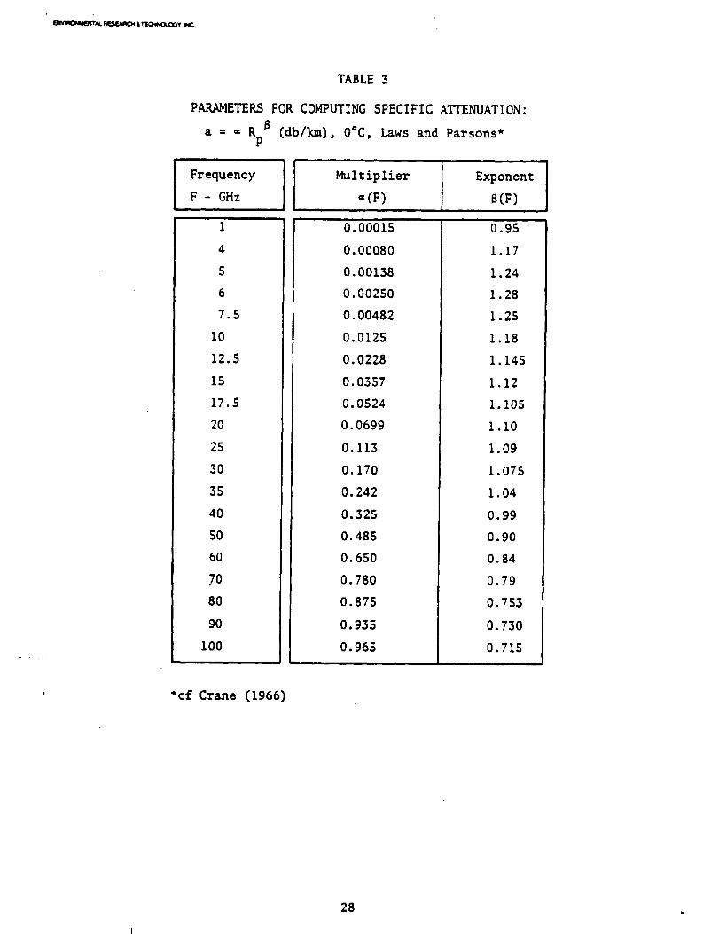
The specific attenuation may be calculated for an ensemble of rain
drops if their size and shape number densities are known. Experience
has shown that adequate results may be obtained if the I.aws and Parsons
(1943) number density model is used for the attenuation calculations
(Crane, 1966} and a power law relationship fit to calculated values to
express the dependence of specific attenuation on r_in rate (Olsen et.
al., 1978). The parameters a and 8 of the power law relationship:
a = aRp B(2)
where a = specific attenuation (dB/km)
Rp = point rain rate (mm/hr)
are both a function of operating frequency. Figures 14 and 15 give the
multiplier, a(F} and exponent B(F), respectively, at frequencies from 1
to 100 GHz. The appropriate a and B parameters may also be obtained
from Table 3 and used in computing the total attenuation from the model.
The total attenuation is obtained by integrating the specific atten-
uation along the path. The resulting equation to be used for the esti-
mation of slant path attenuation is:
25

U_
L_m
dG_m
d
1.0
0.I
.01
.001
.........00010 20
Figure 14
40 60 80 I00F- FREQUENCY (GHz)
Multiplier (,,) in the power law relationship
between specific attenuation and frequency
26I

|
I_.: ---
I I I I
CxJG
--IN3NOdX3
00m
0CO
• pl U,.1=
0 O"
N ,_
O-r _="c.O (_9 ,_
m c:,-* 0
.,-4
>- _t.D
IIJ 4,0
D _._,I
U
UJ
LI. e_
0 _Pd =°p,,l
0
27
PARAMETERS
Ba=_RP
i
Frequency
F - GHz
1
4
S
6
7.5
I0
12.5
15
17.5
2O
25
3O
35
40
5O
60
70
8O
90
I00
ii
TABLE
FOR COMPUTING
(db/km), O°C,
Multiplier
(F)
0.00015
0. 00080
O.00138
0.00250
O. 00482
0.0125
0.0228
0.0357
O. 0524
O. 0699
O. 113
O. 170
0.242
0.325
0.485
O. 650
0.780
0.875
0. 935
O. 965
3
SPECIFIC ATTENUATION:
Laws and Parsons*
i
Exponent
_(F)
0.95
I. 17
1.24
1.28
1.25
1.18
1.145
1.12
1. 105
1.i0
1.09
I.075
I .04
0.99
0.9O
0.84
0.79
0.753
0.730
0.715
*cf Crane (1966)
28
ENV1RONMIENTAI RF.SF-ARCH & TEC_iNCKGGv I_C
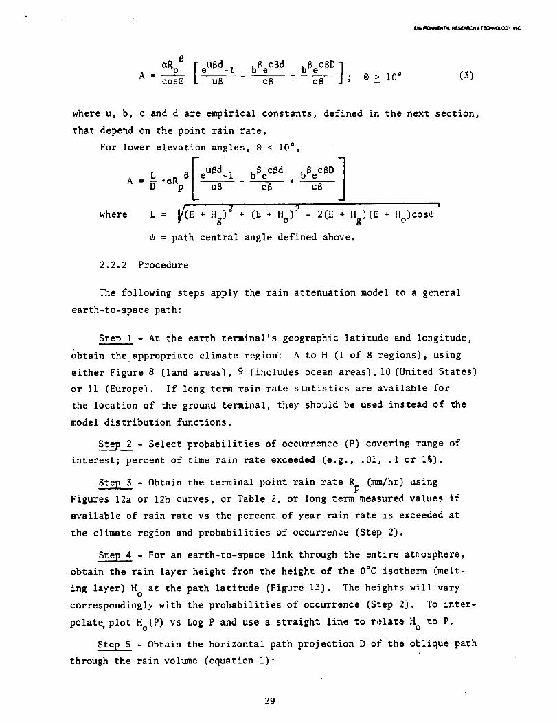
eUBd_ 1
cos@ bBeC8 d bBeCB D ]cB + .cB ; O _ i0 ° (3)
where u, b, c and d are empirical constants, defined in the next section,
that depend on the point rain rate.
For lower elevation angles, ® < I0°,
r jL euBd i bBe cBd bBe cBD
A = 5 "aRp BL cs+ cowhere
)2 2(E + Hg)(E + Ho)COS_L = E + Hg) 2 * (E + H° -
= path central angle defined above.
2.2.2 Procedure
The following steps apply the rain attenuation model to a general
earth-to-space path:
Step 1 - At the earth terminal's geographic latitude and longitude,
obtain the appropriate climate region: A to H (i of 8 regions), using
either Figure 8 (land areas), 9 (includes ocean areas),10 (United States)
or ii (Europe). If long term rain rate statistics are available for
the location of the ground terminal, they should be used instead of the
model distribution functions.
Step 2 - Select probabilities of occurrence (P) covering range of
interest; percent of time rain rate exceeded (e.g., .01, .1 or 1%).
Ste_3 - Obtain the terminal point rain rate Rp (mm/hr) using
Figures 12a or 12b curves, or Table 2, or long term measured values if
available of rain rate vs the percent of year rain rate is exceeded at
the climate region and probabilities of occurrence (Step 2).
Step 4 - For an earth-to-space link through the entire atmosphere,
obtain the rain layer height from the height of the 0*C isotherm (melt-
ing layer} H° at the path latitude (Figure 13). The heights will vary
correspondingly with the probabilities of occurrence (Step 2). To inter-
polat% plot Ho(P) vs Log P and use a straight line to relate H° to P.
Step S - Obtain the horizontal path projection D of the oblique path
through the rain volume (equation I):
29

f
8_vuK_qn_J,_'au. Rf._JUm04 & _v a_C
H - H_D = tane ; 6 _ I0 °
H = height of elevated terminal* (km); H < H0
Hg = height of ground terminal (km)
8 = path elevation angle
*Note: H = H° for earth-to-space links (from Step 4) and H° will
vary with the probability of occurrence, H = H (P).O O
Step6 - Test D _ 22.5 km; if true, proceed to the next step. If
D > 22.5 km, the path is assumed to have the same attenuation value as
for a 22.5 km path but the probability of occurrence is adjusted by the
ratio of 22.5 km to the path length:
new probability of occurrence, P' = p(.22.5 km.)D
where D = path length projected on surface (>22.5 km)
Step 7 - Obtain the parameters a(F) and _(F), relating the specific
attenuation to rain rate, from Table 3 or Figures 14 and 15, or equi-
valent observed data where:
F = operating frequency (GHz)
Step 8 - Compute the total attenuation due to rain using Rp, a, B,
O, D (equation 3):S
R _eUBd 1 bBeCSd b_eCBD ]A./_p_cos8 t. _'B c8 ÷ cS ; e >_.I0"
where A = total path attenuation due to rain (dB)
a,B = parameters relating the specificBattenuation torain rate (from Step 7), a = _R = specific atten-uation P
Rp = point rain rate (Step 3)
0 = elevation angle of path
D = horizontal path distance (from Step 5)d < D < 2_..5 km
30

_NT_I. RESF-A4_.._ & TEO.W_QLOGV I_C
u, b, c, d are empirical constants:
u = In[be cd]d
-0.17b= 2.3R
P
c = 0.026 - 0.03 in RP
d = 3.8 - 0.6 in RP
or alternatively: (if D < d),
_R B [eUSD i]A = __2_cose[
or if D = O, 0 = 90 °,
A = (H - Hg)[CtRp 8]
2.2.3 Comparison with Experiment
Recent observations using the CTS, COMSTAR and ATS-6 satellite
beacons allow the evaluation of the model at a number of frequencies and
locations in regions D2 and D3 of the United States. An example of
observations at CTS at 11.7 GHz (Ippolito, 1979) together with model pre-
dictions is given in Figure 16. The observations match (within 1 dB) the
region D2 model between .015 and .024 percent of the year, match the
tailored distribution between .012 and .02 percent of the year, and match
the measured rain rate distribution over the .005 and .02 percent range.
Since, on average, the two-year distribution is expected to be within 27
percent of the model distribution at 0.01 percent of the year and 33 per-
cent of the model at 0.001 percent of the year, the data are replotted in
Figure 17 on a percentage basis to better assess the agreement between
measurement and model. In this figure, agreement is evident at percen-
tages of the year smaller than 0.04; the region D2 model is within the
expected uncertainty range, the tailored-rain rate model provides better
agreement with measurement, and the measured rain rate data provide the
best attenuation estimate. The measurements show significant disagree-
ment in the .04 to 1 percent range. Since the attenuation values
expected in this range are less than 6 dB, the calibration uncertainty
(.5 dB) and the data quantization used to generate the cistribution {2 dB)
may affect the comparison.
31

O3G')
rn
_0c_
0X
Z0
.I
\
\\
*\
\
\\\\\\\
\
\\
\\
\
11.7 GHz- CTSGREENBELT, MD. ( e = 29 °)
* OBSERVATIONS 1977 & 1978197719787/76 - 12/780
--MODEL (Dz)---MODEL ADJACENT
REG IONS (Dr 18_ D3 )_.4 MODEL MATEDEVIATION FOR 2 YEARSOF OBSERVATIONS
----MODEL USING RAIN RATEDISTRIBUTION FORWASHI NGTON, D.C.
-I--MODEL USING MEASUREDRAIN RATE DISTRIBUTION
STANDARD
\ Dak
\
\
i.-r
itl>..
I..1_0
I--ZLIJt,Jn.,,,i
.01
.001
\\
\
\\
\
\
%
\ •
\\ •
\
0 i0 20 50
ATTENUATION (dB)
Figure 16 Comparison of CTS aEtenuation observations at
11.7 GHz (after Ippolito) with model estimates
5_
,v

I00
!I , !
0 0 0o o
I
(%) 7300_ I (7300_ --03A_3$80)-73001AI V_OWJ NOIlVlA30 1N3OW3d
c'_ W .,_ m
.L.LJ I_ J _ _
0.__ °=
z ._
8
$3

E,I_MmQPeJt_,dTJ_. _ 8 _Y mC
Comparisons between a larger sample of observations and model cal-
culations are presented in Figure 18. The data presented in this figure
include the comparison already presented in Figure 17, 11.7 GHz CTS
observations from Waltham, MA (Nackoney, 1978), Holmdel, N.J. (Rustako,
1979), Blacksburg, VA (Stutzman and Bostian, 1979), and Austin, TX (Vogel,
1979); 19.04 GHz and 28.56 GHz - C0_TAR observations from Holmdel, NJ
(Arnold et al, 1979), Clarksburg, MD (Harris and Hyde, 1977), Wallops
Island, VA (Goldhirsh, 1979) and Blacksburg, VA (Stutsman and Bostian,
1979); and 20 and 30 GHz-ATS-6 (Ippolito, 1976). These data show good
agreement between measurement and model for percentages of the year less
than 0.I; on average the observations deviate from their model predic-
tions by less than eight percent. The rms deviation of all the measure-
ments about the models is 25.7 percent, in agreement with the 29 percent
rms expected uncertainty (at 0.1 and .01 percent of the year).
If all the data are used, the rms deviation increases to 48 percent.
The data for the entire range are strongly affected by the large uncer-
tainties associated with the Blacksburg measurements at percentages
greater than 0.i percent. Since the Blacksburg and Rosman measurements
are for relatively high stations (0.7 km at Blacksburg, 0.88 km at Rosman)
in close geographic location (although differing rain climate subregions),
the good agreement at Rosman and the other stations and poor agreement at
Blacksburg at percentages greater than 0.I percent may indicate instru-
mental difficulties in this percentage range. A review of the calibra-
tion procedures used at Blacksburg indicates that the probable cause of
uncertainty is the use of monthly calibration constants to process all
the data acquired within the month; the daily variation in calibration
could produce the relatively high attenuations in the 0.1 to one percent
range. It is noted that excepting the data from Blacksburg, the compari-
son between observation and measurement is excellent, with less than a
25 percent rms difference over the entire percentage range for frequen-
cies of 19 GHz and above and less than 26 percent rms for all frequencies.
The agreement between observations and climate region model predictions
are within the 29 percent ms deviation value expected for a one-year
set of observations.
Re slant path attenuation model provides attenuation estiEuates
at all possible elevation angles. The sun tracker observations made in
34

I I
8 oo04
-(]_IA_I3S_IO) --13001AI
!!
!!
I!
!!
?
NOI.L_IA30
0
±N39W3W
35

the early seventies provide data for comparison with elevation angle
dependence estimates. Kinase and Kinpara (1973) provided data on the
elevation angle variation of 11.7 GHz attenuation observations for Klang,
Malaysia (climate Region H). The model calculations for I0 and 20 mm/h
(0.66 and 0.33 percent of the year respectively) are presented as a func-
tion of elevation angle in Figure 19 together with the observations for
the same probabilities of occurrence. The model results and measurements
show definite departures from a simple cosecant of the elevation angle
dependence at both high and low elevation angles. The model agrees with
observation at the rms deviation expected for observations which vary in
elevation angle in synchronism with the sun (53% rms). The data for all
elevations and both probabilities of occurrence have a 48 percent rms
deviation about the model predictions; at elevation angles above i0°, the
rms deviation is less than 36%.
These data show excellent agreement between the prediction model
and observations on slant paths through the atmosphere.
A set of comparisons for a 20-km point-to-point path between modeled
and measured attenuation values (Valentin, 1977) are presented in Figure
20. Good agreement between the model estimates and measurements are
evident at all but the highest frequency. In these observations, the
59 GHz measurements clearly have some problems in that the attenuation
at 29 GHz exceeds that at 39 GHZ for percentages of time larger than
0.3%. Also, difficulty is evident at the lower frequencies at larger
percentages o£ the time when the attenuation at 15 GHz exceeds the value
at 29 GHz. For measurements in the 20 to 40 dB range, agreement between
the measurements and model estimates is excellent except at 30 GHz. For
these observations, the dynamic range was not sufficient to make obser-
vations at 0.001 percent of the year at 19 GHz and higher frequencies on
a 20-km path.
2.3 Scintillation
The propagation effects classified as scintillation-producing are
attributable to two regions of the atmosphere. Though generally con-
sidered secondary to theeffects due to molecular absorption and rain
attenuation, the fluctuation losses may, under certain circumstances,
impact significantly on earth-to-space communication paths. The effects
36I

nnn_
o
p-<_
Z0m
I--
Z
I--
A
Z0
ZLO
F-
0
rr
I0
.I
11.8 GHz-MODEL-REGION H
I0 mm/h (0.66%-----20 mm/h (0.34%
"---COSECANT
OF YEAR, ATTEN (45o) . 2.4d B)OF YEAR,ATTEN (45°)=4.7dB)
(ELEVATION)
MEASUREM ENT- KLANG, MALAYSIAo---.o I Omm/h
_-..A 20mm/h1 Ii
0 50 60ELEVATION ANGLE (deg)
Figure 19
9O
Elevation angle dependence of II.8 GHz suntrackerobservations at Klang, Malaysia (Climate Region H;
after Kinase and Kinpara} compared with model
estimate
37

!_"_Ill_III_,N. IILMAIIO4 I, _.O,_y _C:
RAIN ATTENUATION 20 km PATHREGION C (VALENTIN , 1977)
4or '_ • ¢\/ _ _ • "0 "
3o_o, ,,,._ ,\._\./ %\",'\" "_\o___zol. \'k" '¢ '_
,o ,,,,,,,,.o.
.0OOI O.OI IPERCENT OF YEAR ATTENUATION VALUE EXCEEDED
FREQUENCYGHz12.6 o1519 "29 •39 o
MODEL
OBSERVATION
I I
_Omin
e_
Figure 20 Comparison o_ point-to-point observations at five
frequencies on a 20-km path with model estimates
38

F._V)RCNMENTA_. RESF-APX_'_ & TECb4N(_.Q(_Y INC
produced by both the troposphere and ionosphere, sometimes termed signal
fluctuation (or fast fading), are caused by inhomogeneity in the index of
refraction along the propagation path; under extreme conditions, this
inhomogeneity may result in internal atmospheric multipaths. The tropo-
spheric effects are produced in the lowest altitude region (first few
kilometers) of the path by local features such as high humidity gradients
and temperature inversion layers leading to small height intervals in
which the refractive index profile departs markedly from the expected
general exponential decrease with altitude. To a first approximation,
the refractive index structure is horizontally stratified and the regions
of departure appear as thin horizontal layers. Superimposed on these
layers, the refractive index at a particular height will change slightly
in an oscillatory manner due to internal waves and in a random manner due
to turbulence. The internal multipath effects producing fast fading are
experienced when rays propagate over a considerable distance at highly
oblique angles through the near-horizontally-oriented smaller scale
inhomogeneities. Though this usually affects line-of-sight propagation
more at low elevation nngles [below 5° elevation at frequencies below
X-band), the amplitude fluctuations depend on wavelength and may signi-
ficantly affect higher frequencies [above I0 GHz) at increasingly higher
elevations. The effects are seasonally dependent and are variable from
day-to-day as well as geographically.
2.3.1 Ionospheric Scintillation
Ionospheric induced scintillation, also produced by inhomogeneity
in the ionospheric refractive index due to electron density irregulari-
ties, is mostly produced near the height of the maximum electron density
(F-region) of the ionosphere. Again, this may be experienced at low
elevations where much of the ionosphere is traversed or at any elevation
when disturbed ionospheric conditions [such as those cl_ssed as "spread-F")
are experienced. There are particular geographic regions where such
conditions prevail (e.g., equatorial regions or high latitudes where the
propagation paths intersect the auroral zones) and become significant in
path selection and/or design. The ionospheric scintillation effects are
predominately a "lower frequency" effect due to the 12 frequency depen-
dence of the refractive index in ionized regions and are commonly exper-
39

E.qV_ONME_J_. RESE,_C_ • TEO_I._y
ienced only below 4 GHz. The effects, related to electron density
irregularities are variable diurnally, seasonally, and depend on the
current sun spot number of the solar cycle. Additionally, solar-geophys-
ical distrubances affecting the earth's geomagnetic field may influence
the occurrences. For most systems operating above I0 GHz, the amplitude
scintillation and absorption effects due to ionospheric contributions
are secondary to other system error budgets and may be neglected. For
more specific information on the character of signal effects related to
ionospheric scintillation and the impact on transionospheric system_,
several references may be consulted {Crane, 1977, 1978, 1976a), including
a discussion in CCIR Repoz_c 263-3 {1976). In particular, for any pro-
pagation links or services planned at the equatorial or high latitude
locations using lower frequencies, a study of the effects due to pene-
t-ration of the ionosphere should definitely be made.
2.3.2 Tropospheric Scintillation
Tropospheric induced scintillation effects result in several propa-
gation characteristics which may be of significance at the higher fre-
quencies. The three effects of significance to the higher frequencies
at greater elevation angles are the angle-of-arrival and amplitude fluc-
tuations produced by inhomogeneity in the clear-air refractive index,
and the antenna aperture {signal gain) degradation relatable to the
finite scale sizes of the irregularities. The angle-of-arrival effects
produce a slight angular variation of the received signal about the
apparent angular position {also affected by average refractive bending)
of the rays from the satellite source. The elevation angle variations
are typically I0 times larger than the azimu_al variations. Data
obtained from satellite observations made using a large aperture track-
ing antenna at Haystack Observatory, Westford, Mass. {at X-band), suE-
gests that angle scintillation is not likely to be important for antenna
beamwidths larger than 0.3" at all elevation angles or beamdwidths larger
than 0.01 a at all elevation angles higher than I0°. The elevation angle
fluctuations are of the same order of magnitude as the expected uncer-
tainty in refraction correction using surface refractivity values. Fig-
ure 21 (Crane, 1976b) indicates the range of extremes in the RMS fluctu-
ations in elevation angle versus elevation on the 120 foot {56.6 m)
40

EN_IqO_JEN TN. FtE_E_CJ'f & TIr(_'_OL_¥
0.1 100
i "3GHz
C
I It 10
APPIII_NT II.[V£TION ANGt.[ till)
Figure 21 RMS fluctuations in elevation angle for a full year
period
100
I0
|
CLI
Figure 22
.__, 7.3GHz
. "__ -_/suuurn
°• SPlltmG .- D •
• SUMMI['m
0 FALL
i W INTI[]I
i i ' _ * _'_1 .. | I ' i = _ ,,_1 I ,I I I _ l'_
I IO I00
AIIPAIIIIL'IIT rlJL'YATION AI_I.J[ (lleql)
Median RMS fluctuations in elevation angle by season
4l
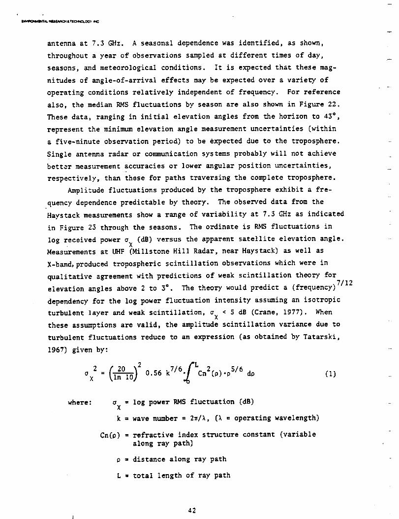
antenna at 7.3 GHz. A seasonal dependence was identified, as shown,
throughout a year of observations sampled at different times of day,
seasons, and meteorological conditions. It is expected that these mag-
nitudes of angle-of-arrival effects may be expected over a variety of
operating conditions relatively independent of frequency. For reference
also, the median RMS fluctuations by season are also shown in Figure 22.
These data, ranging in initial elevation angles from the horizon to 43 °,
represent the minimum elevation angle measurement uncertainties (within
a five-minute observation period) to be expected due to the troposphere.
Single antenna radar or communication systems probably will not achieve
better measurement accuracies or lower angular position uncertainties,-
respectively, than these for paths traversing the complete troposphere.
Amplitude fluctuations produced by the troposphere exhibit a fre-
quency dependence predictable by theory. The observed data from the
Haystack measurements show a range of variability at 7.3 GHz as indicated
in Figure 23 through the seasons. The ordinate is KMS fluctuations in
log received power a (dB) versus the apparent satellite elevation angle.X
Measurements at UHF (Millstone Hill Radar, near Haystack) as well as
X-band, produced tropospheric scintillation observations which were in
qualitative agreement with predictions of weak scintillation theory for7/12
elevation angles above 2 to 3°. The theory would predict a (frequency)
dependency for the log power fluctuation intensity assuming an isotropic
turbulent layer and weak scintillation, a < 5 dB (Crane, 1977). WhenX
these assumptions are valid, the amplitude scintillation variance due to
turbulent fluctuations reduce to an expression (as obtained by Tatarski,
1967) given by:
2 [ 20 kT/6. Lcn2(p) pS/6o = 0.56 • do (i)x Lln lo/
where: o = log power RMS fluctuation [dB)X
k = wave n,,mber = 2_/X, CX = operating wavelength)
Cn(p) = refractive index structure constant {variable
along ray path)
p = distance along ray path
L = total length of ray path
42I

ENVII_I_IENTAL _F.SE,_qCI_ & TEO'INOI._'_ I_
Precise knowledge, therefore, of the amplitude flu_:tuation depends
on a knowledge of the refractive index structure function along any
given oblique path. Since this is usually unknown in detail, approxima-
tions would need to be made to model Cn 2 for a specific location. At
10 GHz, the signal may fluctuate at levels between 0.1 and about 1.0 dB
depending upon elevation angle and conditions (see Figure 23) with the
requirement that elevation angles are above about 3 degrees. At 100 GHz,
the levels scale in frequency to lie correspondingly between 0.4 and
3.8 dB, depending on elevation angle and upon (low or high) fluctuation
conditions if the refractive index structure is invariant over the fre-
quency range.
The third tropospheric effect of significance, antenna aperture
degradation, is dependent on the scale sizes of the refractive inhomo-
geneities relative to the antenna diameter. The effect, sometimes
expressed as antenna gain-loss, occurs because the antenna aperture and
the propagating medium are coupled. For a propagation path traversing
the troposphere to a distant satellite, the Presnel zone sizes may be
defined as:
F : (2)
where: n : order of Fresnel zone
z : the reduced path length
= p.(L-p)L
L = total length of ray path
0 = position along ray path
= operating wavelength
When the scale size of refractive index irregularities L° is small
compared to the Presnel zone size, the scattering can be described as
isotropic and weak scattering theory as described holds. The scattering
mechanism is usually classed as small scale turbulence. At higher micro-
wave frequencies, L can become larger than the Fresnel zone causingo
anisotropic scattering and considerable spatial curvature of the incident
wavefronts. For increasingly large antenna apertures, a size, D, is reached
at which the antenna gain, predicated on a plane wavefront, is degraded.
43

i
&
o.m
Figure 23
10.0
1,0
0.1
0.010.1
Figure 24
I ,, i0.1 1 _O 1_
IIII_NT [4[VATION AN@L_ |Mq)|
RM5 fluctuations in log power (dB) for a full year
period
\\
*lOiS[ L[VI_O.4rd4s
[xpl[c'r[g [LE_ATI_I JUiGI.[D[PI[NOI[N¢I[ Of A TUI_IUI_NTI.AVtiq AT l*m MI[IGI4T
! !
API_R[NT [L[V_ION ANGL[ |_||
RMS fluctuations in log power at X-band and UHF,
2g-30 April 1975
44

ENVIROI_YlF_NTAL RESEARC,_ & TEC_INO.OG Y tNC
With further curvature, some of the fluctuations due to a corrugated
wavefront are spatially averaged by the antenna. Further, as the eleva-
tion angle increases, the Fresnel zone size (given by Eq. 2) continues to
decrease due to the rapidly decreasing distance o between the producing
layer and the antenna. Re result is therefore a reduction in the fluc-
tuation depth due to antenna averaging and a reduction in the effective
antenna gain (i.e. gain-loss). Pun example of this effect occurring, is
shown in Figure 24 for the Haystack 36.6 m antenna. _"nere was a fall-off
in the 7.3 GHz PJ_S fluctuations from the level predicted (dashed line),
as the elevation angle increased above two degrees, until the fluctua-
tion level at 10 degrees reached that obtained at UHF. For the predic-
tion, a turbulent layer height of 1P_m was assuJned. Tatarski C1967)
showed that the RMS fluctuations are reduced by 20 percent when the dia-
meter of a unifo_nnly weighted circular aperture is one-half the first
Fresnel zone size (D = _V_-z--/2).
The tropospheric scintillation model presented is based upon the
Haystack measurements and the theory described. An assumed average
height of 1 km was used to a thin turbulent layer. The rms fluctuation
level used as a reference point for the model col-responds to the annual
mean at one degree elevation obtained at Haystack Observatory. As a
result of the theory and a cosecant 8 power law fit approximation for a
1 km high layer, the following £1uctuation model dependencies were
obtained for the model:
where:
85
I G{R) _l/2(dB)G (R} REF }
(3)
°x,REF= reference rms fluctuation at 1°, 7.3 GHz,
Haystack, D = 36.6 m (dB)
{o = 1.883 dB is used iP the model}x,REF
F = operating frequency (GHz)
8 = apparent elevation angle
G(R) = antenna aperture averaging factor,
Tartarski (1967)
G(R)REF = value for Haystack at 1°, D = 36.6 m
45

_M_3_LNVAL Af.Wau_O_ • _O_J3Qy
A piecewise linear approximation to Tartarski's antenna aperture
averaging factor, G(R) was made as follows:
G(R) = 1.0 1.4_- ; O<< 0.5
= 0.5 - 0.41_ _;0.5<
R-- <1.0
,/re-{4)
where:
=-0. i ; 1.0<R
i
R = effective radius of circular antenna aperture (m)
1/2 D= (n) _ , D = physical diameter of reflector
and n = antenna efficiency factor {n = 0.56,
{n) 172" = 0.75 assumed in model}
L = slant distance to height of a horizontal thin
turbulent layer
= [h2 ÷ 2 r h ÷ {re sine)2] I/2 - r sinee e
h = height of layer {h = I000 m assL,ned in model}
re
= effective earth radius including refraction
{r = 8.5 x 10⁶m in model}e
k = operating wavelength (m)
where:
For computational purposes, equation [3) reduces to the following:
aX(F,$,D) = K.F 7/12 Ccsc9} 0"85 (G(R)) 1/2 (dS)
K = 2.5 x 10 -2
CS)
The model has been tested successfully against several sources of
experimental observations exercising the frequency, elevation angle and
aperture dependencies. Figure 25 shows the model compared with the
annual mean 7.3 GHz data beyond the reference point value. A very good
fit is observed with elevation angle. For comparison, the data for a
specific recording period from Figure 24 is included which departs from
the mean bur lies within the uncertainty bounds. The Millstone 0.4 GHz
46

F_NVIROI_/n¢ h'l"kl. FI I:'$_t.,kRC;N t, tE(_I.II_IIOI.(_G_t i1_
10
1.0
O3
V
0.1 "
0.01O.
, , CRANE, 1976 bHAYSTACK, D=36.6 m( • ) 7.3 GHz, 4/29--
T REFERENCE 30/75,. I T/POINT ",It7.5 GHz ANNUAL
FOR MEAN, +_.I o"
I'lL. MODEL MILLSTONE, D=25.6m_, (,) 0.4GHz, 4/29- _
• 30/75MODEL:
7.3 GHz
_| i I i i • i i i i i i
1.0
ELEVATION ANGLE
Figure 25
i • I I I I
I0
(deg)
Comparison of tropospheric scintillation model withHaystack (7.3 GHz) and Millstone (0.4 GHz) observa-tions
9C
47

_l_,_k mE.,_lVJ_tO,g &_-C>egCI.CGV _.
data for the same period is shown compared with the model curve a¢ this
frequency. The 4 and 6 GHz data obtained in Japan by Yokoi (1970) are
compared with the model predictions in Figure 26 over the elevation
angle range of 5 to 50 degrees. Again, a favorable match occurs between
the observations and the model.
Finally, the ATS-6 measurements are compared with the model over
the frequency range of 2 to 50 GHz. Figure 27 shows the Ohio State
University measurements, Baxter and Hodge (1978), at 2 GHz (D = 9.1 m)
and of Hodge, et al (1976) at 20 and 30 GHz (D = 4.6 m). In this figure,
the data are shown in terms of amplitude variance (S2] as opposed to rms
log power. The conversion for small amplitudes is:
S2 = 20 loglo (dB) (6)
The model curves agree well with the measurements expecially at 2 and
30 GHz over the elevation angle range from 1 to 45 degrees. The model,
therefore, appears generally applicable over a wide range of the para-
meters to predict the rms fluctuation losses, on average, to be expected
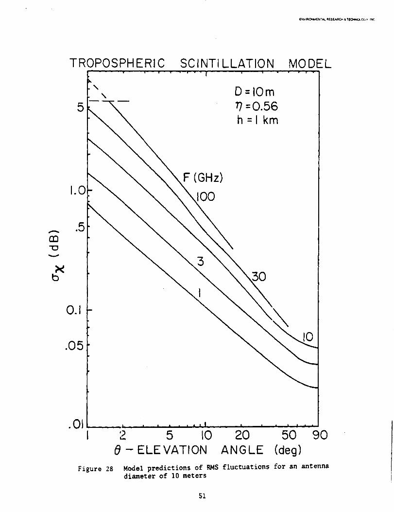
at any location. Figure 28 depicts a specific family of curves using
equation (5) for a fixed antenna aperture diameter D, of ten meters.
2.3.3 Procedure
To estimate losses due to tropospheric scintillation Lscint(dB),
the following steps may be used:
1 - Obtain a value of R/_to test the region ofStep aperture
averaging in equation (4). The antenna diameter D, elevation angle B
and the operating wavelength, k = c/F, are required input variables.
Step 2 - Compute the appropriate aperture averaging factor G(R)
from equation (4), depending on the range of R/_ from step I.
Step 3 - Compute the tropospheric scintillation loss Lscin t =
_X(P,e,D) using equation (5). Note that a correction for elevation
angle-of-arrival fluctuations is not needed if the antenna beamwidth is
larger than that indicated by the maximum values in Figures 21 or 22.
48

V
0.5 _,_ MODEL: Io4_.,..._ (--) 6.39GHz0.::5
0.2
0.1
0.05
_Oo_, ....°o_o_,-?,,o. 4.17GHz
m
o ()'_
(
o-._0 .
0 0
Ci
6 8 !0 20 50 50
ELEVATION ANGLE (de9)
YOKOI, 1970D=22m( o ) 4.17 GHz( • ) 6.::.59GHz
Figure 26 Comparison of model predictions with observationsat 4 and 6 GHz (after Yokoi)
49

E_V;_A_. RESF..A_01 & TEC;'eN(_,OGV _C
(SP) 39NVlN_A 3(]n.LlqcllAIV _S
SOI
ENVAIqONM_NTA_. RESF.AACZ,4 & TEO'INOL_."* V Ir_C
TROPOSPHERIC
_\ " , ,
5\
SCINTI LLATION MODEL• • • T • "l ' " " •| i • • • w •
I
D=iOm=0.56
h=lkm
1.0F (GHz)
I00
m
V
0.I
5
\
.01
Figure 28
L, ,, I | | • • • I | a i _ k I ,
2 5 I0 20 50 90
I_ - ELEVATION ANGLE (deg)
Modet predictions of P_dS _luctuations £or an antennadiameter o£ 10 meters
51

°
2.4 Low Elevation Angle Effects
Observations of slowly setting satellites (Crane, 1976b) show that
strong signal amplitude fading (or scintillation) occurred at elevation
angles below 2 to 3 degrees due to the troposphere. The strong fading
(greater than 5 dB) was a result of a number of randomly occurring
multipath events which produced accompanying angle-of-arrival scintilla-
tion. During the strong scintillation multipath events, signal depolar-
ization was noted. The change in apparent polarization was presumed to
be caused by the response of the antenna (Haystack, 36.6 meter diam.,
7.3 GHz) to the multiple signals received at slightly differing angles
of arrival. These propagation effects are dominated by large scale
refractive index perturbations or layers. They are to be distinguished
from weak scintillation effects not only because of larger fading depths
but characteristic slower fades, low elevation angle occurrence (below
3 degrees (McCormick and Maynard, 1972) and the associated angle-of-
arrival effects,
Another low angle effect of significance to earth-space paths is
that due to defocusing (divergence) of the near-horizon rays due to the
average atmospheric refractivity profile. Though not a large attenuation
effect (order of I dE at one degree elevation), an average defocusing
persists and should be factored into system margins for geometry involv-
ing the low angles.
2.4.1 Atmospheric Multipath
It has generally been accepted and substantiated for microwave
point-to-point transmission paths that the mechanism for severe fre-
quency-selective fading is attributable to multiple paths produced within
the troposphere by refractive layers {Ruthroff, 1971). The multiple
path fading mechanism is also responsible for the low elevation scintilla-
tion effects on earth-to-satellite paths (Crane, 1976b; McCormick and
Maynard, 1972]. Data from Ottawa, Canada (McCormick and Maynard, 1972)_j
have been compiled on a seasonal basis as shown in Figures 29a to _, in
terms of percentage distribution. The data base consists of 654 hours
of observation on a 9.1 m tracking antenna at elevation angles between 0
and 8 degrees (one degree increments) during the period 1967-1971, grouped
into four seasons as indicated. The data were normalized to an "unper-
52

FJCVIII_I_ENTAL RE SF-A/:IC_ & TEC)-INOt_ Y
i,I I, (DZ
<. -_ "__,_.,
-- - _ i _"
- //AI Is_ o_ • o o >i::t,.,,+ 1 +'-+°"0' - +I +I +"+"e/i//il l :°<,.o°, _ 1°, . , .... . , , ,_ "__ _ o _, _, _ ®<_ o+ ®<_.I I '_ t_ O'_
ooE
_ _,_=c_ _O'lI,,i.I _=<_
• ,, . _ "' = <..> _ ._._
_ l.i.l <I_ _ m..+-, m
g// t+#ill ... _ jo
I/lli +I °.'+=' iiJJJJ[////1 <- t +_ ///llkll + l<_
I "'i " " I I " _:_ I _" I '' " I I I I
m ¢ o ? ? _,. ® _" o ¢ _ m
(8P) ICl3111 C]':IgI:IPIII:I3dNI7 Ol":JAIIV731# 7":iA'47 7VNOIS
$3

turbed" 15-minute median signal level (i.e., the median level that would
occur in the absence of the fading). The IS-minute period is long enough
to contain several of the longest-period fades, and short enough to
remove changes in median level due to the motion of the satellite (some
were near-geostationary with a slow drift). It is apparent that fading
is much worse in sLmuner months than in the winter, with spring and fall
intermediate to these extremes. For elevation angles less than 4 degrees,
the system margin required to overcome fading undergoes a rapid increase.
A sample set of the 15-minute period median level data is shown in Figure
30 as a function of elevation angle. Approximately 300 hours of measure-
ments are shown from Ottawa during a three-week period in October and
November 1970 {McCormick and Maynard, 1972). The dashed line represents
the median signal level in the absence of losses. The solid line indi-
cates the calculated effect of focusing losses due to regular refraction.
The highly nonlinear departure from the solid curve below 3 degrees is
attributable to the strong fading due to atmospheric multipath although
some ground multipath may influence the measurements below one degree.
Figure 51 shows the combined seasonal and elevation effects on fading
depth at the 99.9 percent of time exceeded level. The latter provides a
means of estimating system fade margins primarily attributable to the
low elevation atmospheric multipath effects to be expected over continental
locations. For a fixed path length, the fading attenuation distribution
would be predicted to go as i/k (k = free space wavelength) (Ruthroff,
1971). Therefore, an adjustment of fading depths with frequency may be
made but exercised with caution, at the users option, due to a pausity
of supporting observational data.
2.4.2 Spreading Loss
Signal loss may also result from atmospheric defocusing (focusing
loss) which arises due to spreading of the antenna beam caused by the
variation of refractive bending with elevation angle at low elevations.
Though this effect may be considered negligible for all elevation angles
above 5° where focusing losses are of the order of 0.1 dB, the loss term
becomes significant below this angle. Figure 32 (Crane, 1976c) shows the
focusing loss through the complete atmosphere due to atmospheric refrac-
tion effects. These results were obtained by raytracing through numer-
54

m"1_ ENYISK;XClV_NTAL RESE_C.J.I &TECH_"_'_'X, v INC
._ -I00 , , , , ,(.9Z ... ,I.IJ - -,',- .4 "" " • ..,,.- " • - ,. _=-los : ,-:-'_ ?.'-. . . " _.-.]
_ "-_.Pk;" .
<E -I IU "1.'>.. "
.::'_"-" /_':: " /
,', "115 -..'z . i',' • 1-> 3 /
n_ 0 I 2 3 4 5 6
ELEVATION ANGLE (DEGREES)
Figure 30 Median signal level as a function of elevation
angle [HcCormick and Ha)mard, 1972]
12 " , ....
B +,\ X SPRING
I0 _ '_ \ + -SUMMER
_ _, ® FALL& WINTER
_4 ' _t, -
2 . '_"
", _ _ ×
0 '' I ' I I '' ' l I I -- l
0 I 2 3 4 5 6 7 8ELEVATION ANGLE (DEGREES)
Figure 31 Combined seasonal and elevation e£fects on £adingdepth at the 99.9 percent o£ time exceeded level.
55

E_RO_cNTAL RESE_O,O• rE_OOY.
100
10
A I
totOO/
Z" i I
tO
OM.
.01
.0010.I
m
D
m
m
Figure
ALBANY DATAAUG. & FEB.
\\
\
-----AVERAGE
------ RMS VARIATION
AVERAGE
• 450N. LAT. dULYSTANDARD+ HUMIDITY
ABOUT--
U.S.
ATMOSPHEREMODEL
\\
\\
\\\
\\\\\\\\\
I IO IO0
INITIAL ELEVATION ANGLE (deg.)
32 Focusing loss and P.HS va¢ia¢ion through the atmo-sphere a¢ low elevation angles due to troposphericrefract ion
56

ous day and night refractive index profiles from Albany, N.Y. over a
several year period. At one degree elevations, the foe:using losses are
about 0.8 dB±0.3 dB. At the horizon, the loss becomes greater than 2 dB
with uncertainties of the same order as the average loss. These effects
may be considered typical of effects observed over inland (continental)
locations. For sites located near coastal areas, islands, at sea, or in
tropical regions, the focusing losses may increase somewhat from these
levels due to increased surface refractivity and different near-surface
refractive index gradients (see also Yokoi, 1970). Focusing losses should
be independent of frequency over the range of 1 to 100 GHz where water
vapor is contributing to the refractive profile. The effects due to dry
air alone and at higher frequencies have not been estimated but should
be less significant.
2.4.3 Procedure
To estimate the system margins for atmospheric multipath and spread-
ing loss at low elevations (below 5 degrees), the following steps may be
used:
Step 1 - Obtain the elevation angle ranges of concern for earth-to-
space path.
Step 2 - Choose percentage of times to be exceeded for selected
system fade margin (e.g., 95%, 99% or 99.9%).
Step 3 - Enter curves of Figures 29a through d (for the four sea-
sons) at appropriate elevation curve and percentages to obtain a table of
fading depths Lfade (dB) versus season and percentage exceeded.
Step 4 - The effect of frequency on fading depth may now be esti-
mated (at the users option):
_dB = I0 loglO[Tf°.-_3]
where: AdB = correction to fading depth due to frequency differentthan 7.5 GHz
f = operating frequency (GHz)op
57

This value may be added to all the losses obtained in the table of Step 3.
It is not suggested to exercise this option for large frequency depar-
tures from 7.3 GHz due to lack of supporting measurements.
Step 5 - Obtain focusing loss Lfocu s (dB) from Figure 32 at the
path elevation angle. This value may be considered a constant to be
added without regard to percentage of time or season.
Step 6 - The maximum of Step 4 and losses from Step 5 may be
retained for the determination of total losses and system margins.
2.5 Radome Attenuation
Though radomes ideally shelter an antenna structure from environ-
mental exposure, some small degrading effects occur due to the radome's
transmission loss which further degrades during periods of rain or wet-
ness on the radome.
2.5.1 Dry Conditions
The transmission losses typically experienced due to a radome over
an antenna vary with material, thickness, and operating frequency.
Typically, the one-way losses (Skolnik, 1970) are designed to be a few
tenths of a dB (0.2 to 0.5 dB typical). In some instances the loss Ldry
may exceed 1 r dB due to the rib construction or the need for a thick
walled structure. Generally, losses exceeding 1 dB are considered non-
optimum designs.
2.5.2 Wet Conditions
A factor often not adequately taken into account in system design is
the additional system margin required due to a wet radome, Lwe t. This
effect is produced by a thin layer of water over the radome material due
to a steady rainfall or dew condition. Losses exceeding j to 2 dB beyond
that of normal radome attentuation may be experienced during rain.
2.6 Diversity/ Schemes
Localized cells of rain attenuation can produce earth-to-space
path attenuations and correspondingly, higher noise temperatures at the
higher frequencies (above 10 GHz) which tax the system margins for
58

_EA_'AL RESF.A.q_ & TEC;HIhIQLCX_Y INC
small percentages of the time. To maintain a required level of relia-
bility [minimum outage time) it may be necessary in some climate regions
to employ site-diversity or large scale spatial antenna separations
thereby avoiding high attenuations over any single path. In order to
design a diversity system for a given location some estimates of rain
cell size and separations is needed. From experiments using satellite
and radiometric paths in diversity configurations, a data base is becom-
ing available in order to estimate system performance and spacing
requirements. It is always somewhat hazardous to generalize a particular
set of empirical results to locations for which no data exists and
caution should be exercised in the adoption of a simple model for a
system design. In addition to direct diversity measurements, weather
radar backscatter experiments are yielding measurements of rain-cell
size and distribution statistics which are increasingly valuable in
diversity system design and estimation.
2.6.1 Earth Terminal Site-Diversity
At any given site location, and period of weather and high rainfall
a cluster of rain cells in an array constituting a storm region, may have
a particular orientation with respect to the weather fronts passing over
the region. The shape and orientation of the storm will have an effect
on the diversity system providing two (or more) alternative paths through
the region. Figure 33 shows a radar measurement of the structure of a
New England sLuTLmer shower (Crane, 1971). The radar used was the Millstone
Hill L-band radar at Westford, Massachusetts having a resolution volume
of about 1 km 5 (Crane, 1968).
The radar map of rain intensity shows several small cells with 10 dB
down widths the order of 5 km across and peak to minimum rain intensity
distances the order of 5 km. The rain rate tabulated along with the Z
(radar reflectivity factor) values is computed from Z e using the approxi-
mate expression Ze = 200 R 1"6. Attenuation coefficient estimates are
also tabulated for 7.78 GHz. Using a model and calculating the attenua-
tion along the ray from the radar through the shower cells, the attenua-
tions estimate given in Figure 34 results. The data are the estimated
values and the lines include the plus and minus rms fluctuations due both
to uncertainties in the radar measurements and the drop-size distribution.
59

ENV_aL RqEUaII04 & Tt-O4_GLOGY
vlW
0
"0
Q3
Z
W0
W
W
aa
w
fa.
60I

ENVlRGNMEWi'AL RESEARCH & TECHNOLOGY R_C
nn"10
ZC)u
I..-
Zu.JI.--I-<C
10
5
• -Estimated value
Lines -RMS uncertainty due to drop-size dist and radar
AIRCRAFT
0270 274 278 282 286 290
AZIMUTH (deg)
24 JUL 1967
7.78 GHz
2052 GMT 1.4-DEG ELEVATION
0 = DROP TEMPERATURE
Figure 34 Esti_ted attenuation using Millstone Hill L-bandradar data
61

i
_easoN_i_A& A_SEARO4 8 TE_OGy
From these results it is seen that the significant amounts of attenua=ion
(i0 dB or higher at X-band) are contributed by small areas of rain, less
than 5 km in extent. Since the cells can be considered to be relatively
uniform columns of rain, several km high, a communication path might
intercept one or more of these cells depending on orientation. Similarly
a set of S-band radar data from Ottawa during 1970 (Strickland, 1974a)
was analyzed statistically to determine cell size distributions and joint
probabilities of occurrence as a function of two path separation dis-
tance. These results showed that 80% of the cells had a size Treater
than 2 km, 50% exceeded about 6 km, and 20% exceeded 14 km extents for an
attenuation level criterion of 5 dB. The attenuations were calculated for
15.5 GHz and compared with satellite (ATS-5) measurements. The cell
separation statistics were distances of about 15, 30 and 45 km for the
three percentages of occurrence exceeded. Recent measurements from
Goodland, Kansas (Crane, 1979) have yielded (5 dB down reflectivity) cell
diameters of about 2.5 km with cell separations of 5 to 6 km for all
cells and 10 to 12 km for significant cell. Storm sizes of 30 to 60 km
in length and I0 to 20 km in width are typically observed nominally agree-
ing with the Ottawa observations.
Given two (or more) propagation paths, the diversity gain, G, is
defined (Hedge, 1974) as the difference in dB between the rain attenua-
tion (A) on a single path and that obtained jointly with diversity paths
(Adiv) at a specified percentage of time exceeded. The diversity gain
is therefore a function of the specified level of percentage of time the
single path attenuation (or fade depth) is exceeded. A compilation of
diversity path experimentaldata at 15.3 and 16 GHz was performed (Hedge,
1974) and is included in Figure 35. Shown is the two-path diversity
gain versus path separation. The parameter in the set of connected data
curves is the single path fade depth in dB produced by rain occurrences
(not regarding the percentage of time the fade depth was exceeded). It
can be noted and defined that diversity gain action begins (Gdi v = about
1 dB) when the single path attenuation reaches about 3 dR. This was
achieved on all paths separated by _ore than 3 km. For a variety of rain
climate region D communication paths at frequencies from 12 to 20 GHz
(see Figures 16 and 18, Section 2.2), the 5 dB attenuation level is
exceeded about 0.2% of the time. Figure 55 shows that most path
62

ENVII_4_NMENTAI. RESF.J_CIH & TIcO'thK_OOY )NC.
63

diversity gain improvement is achieved for paths separated a few km (of
the order of one or two rain cell sizes). Beyond some nominal path
separation, little improvement is achieved for a much larger path
separat ion.
Caution should be exercised before attempting to apply a family of
curves such as Figure 35 or an empirical model extending the concept to
perhaps 30 GHz as suggested by Kaul, et al. (1978). The data base was
limited to experiments in rain climate region D (New Jersey and Ohio).
The model is based solely on attenuation rather than rain rate statistics.
The diversity paths forming the model data base were nominally of the
same configuration; e.g. NW-SH baseline orientation, elevation angles of
35 °, azimuth angles of 220 °, and link frequencies below 20 GHz. There-
fore, the use of the model is not recommended for general application and
for propagation paths departing significantly from the conditions and
not at all for frequencies above 30 GHz.
To analyze the requirements for site diversity separation in rain
climate region D (P _ 30 GHz) one should first proceed with a path rain
attenuation distribution analysis (Section 2.2). Once the single-path
attenuation versus percent of year exceeded curve is obtained, the mini-
mum site (path) separations may be estimated using the IS GHz curves of
Figure 35. The working level of fade depth (attenuation) permissible at
the fading margin designed will thereby specify the diversity path
separation required for protection against outages.
2.6.2 Satellite Terminal Techniques
Since spaced satellites analogous to site-diversity for the purpose
of spatial diversity alone is both impractical from a cost standpoint
and generally incompatible with narrow beam earth terminals it will not
be considered an option. What may be allowable is multiple satellite
paths from one earth terminal using dual antennas. This becomes imprac-
tical for rain occurrences near the earth terminal.
Options that may be open, in lieu of spatial separation diversity
are frequency diversity and time diversity. The former requires shifting
to a lower frequency band (usually at the sacrifice of a reduced infor-
mation bandwidth) when attenuation exceeds the system margin. The latter
also compromises information by some form of repeated message when our-
ages occur.
64
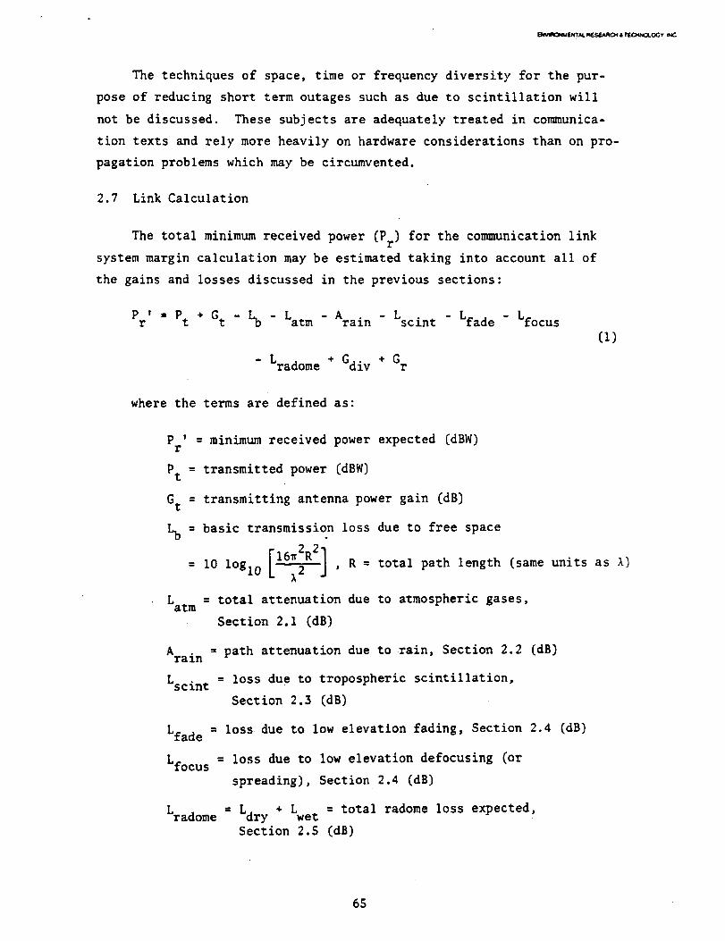
EIea_. SF.._CM & _OGV
The techniques o£ space, time or frequency diversity for the pur-
pose of reducing short term outages such as due to scintillation will
not be discussed. These subjects are adequately treated in communica-
tion texts and rely more heavily on hardware considerations than on pro-
pagation problems which may be circumvented.
2.7 Link Calculation
The total minimum received power (Pr) for the communication link
system margin calculation may be estimated taking into account all of
the gains and losses discussed in the previous sections:
Pr' = Pt ÷ Gt " _ - Lat m "Arain - Lscin t -
- Lradome ÷ Gdi v + Gr
Lfade - Lfocu s
(1)
where the terms are defined as:
P ' = minimum received power expected (dBW)r
Pt _ transmitted power {dBW)
Gt = transmitting antenna power gain (dB)
Lb = basic transmission loss due to free space
[16_2R2l
= I0 loglo L ] ' R = total path length (same units as l}
Latm = total attenuation due to atmospheric gases,
Section 2.1 (dB)
Arain = path attenuation due to .rain, Section 2.2 (dB)
Lscin t = loss due to tropospheric scintillation,
Section 2.5 (dB)
Lfade = loss due to low elevation fading, Section 2.4 (dB)
Lfocu s = loss due to low elevation defocusing (or
spreading), Section 2.4 (dB)
Lradome = Ldry + Lwet = total radome loss expected,
Section 2.5 (dB)
65

t
_At, MI,,U, JAC3M & _OOY _',JC
Gdi v = system diversity gain, Section 2.6 (dB}
Gr = receiving antenna power gain (dB}
r4_Ae_= lO lOgloL- -J
A e = receiving antenna effective aperture (same units
as _2) • n'A
A = physical aperture of receiving antenna
= aperture efficiency factor
Given that a link is required to maintain a specified signal
carrier-to-noise level (R • S/N), the system fade margin (F) may be
considered to be the protection built into the system design against
variable propagation losses:
FdB = Arafn + Lscin t + L£ade + Lwe t (dB) C23
The combined signal-to-noise is:
S/N total = RdB + FdB = Pr - Pn
where:
C33
RdB • required signal-to-noise under worst conditions (dB)
FdB = designed system fade margin (dB)
P = received power under normal conditions (dBW)r
Pn = total received noise power (dBW)
The required system fade margin, combining the fixed propagation
losses (Lp) is therefore:
FdB = Pt " PN + Gt + Gr ÷ Gdiv. " Lp - RdB
where:
C43
LP
= fixed propagation losses
= Lb . Latm. + Lfocu s + Ldry CdS)
66I

3. RECEIVER NOISE
Though natural radio noise can be caused by other sources, the
principal sources are due to atmospheric emission, the radio sky {such as
the sun, Cassiopeia, and Cygnus), earth reradiation, and antenna contri-
butions. These sources are to be distinguished from interference {man-
made noise), a topic requiring separate treatment. The discussion will
be limited to the noise producing the sensitivity limit on surface-based
antennas looking skyward. The principal natural sources of noise emission
are those of a_mospheric origin encountered in the main antenna lobe and
the low elevation energy from earth reradiation entering the side lobes
of the antenna. Specifically, the areas considered will be limited to
the microwave emission of the atmospheric gases, rain emission, and
thermal noise contributions due to the antenna. The radio sky noise
background and scattered energy sources are omitted or assumed to be
sufficiently small to be neglected. Consequently, strong extraterrestrial
noise sources, such as the sun, will be assumed to be out of the main
lobe of the antenna.
Unlike the earth terminal, the satellite terminal experiences radi-
ation from the earth and cloud tops within the main lobe as well as the
atmospheric emissions. With larger antenna beam widths (smaller aper-
tures), the satellite antenna system is usually constrained by other sys-
tem design considerations (beyond the scope of this report) than sensi-
tivity alone. The background noise and man-made interference are insepar-
able when considering the satellite terminal, as opposed to the earth
terminal, and set the noise floor with which the up-link receiving system
works.
3.1 Emission by Atmospheric Gases
The atmospheric gases, water vapor and oxygen, emit energy in the
microwave region of the electromagnetic spectrum. The frequencies at
which emission is strongest correspond to, the absorption bands discussed
in Section 2.1. The sky temperature (Ts) along a ray path can be expressed
{Crane, 1971) as:
67

/sTs = T[S) SCS) exp BCx) dS (1)
where: Ts = sky temperature at given ray angle (°K);
T(S) = kinetic temperature of the gas at a position S aIongthe ray (°K) ;
B(S) = attenuation cross section per unit volume of the gas
at position S along the ray;
= A/tO log e = A/4.34, where A is attenuation coeffi-
cient in dB per unit length.
The power received at the antenna is due to thermal noise or the
apparent antenna temperature {Ta). The apparent temperature is colposed
of several terms including antenna temperature due to atmospheric emis-
sion (TA). To enumerate other sou_:es, Ta has contributions due to extra-
terrestrial noise sources, hydrometeor emission, atmospheric scattered
earth radiation, cloud emission and sources picked up by antenna side-
lobes. If the noise source has an angular area larger than the antenna
beamdwidth, the temperature of this source determines the antenna temper-
ature contribution. The term due to atmospheric emission is expressed
by the integTal over the solid angle:
TA - 1/4_ /4VG(n) Ts(n)_ (2)
where: TA = antenna temperature due to atmospheric emission {'K);
G{_) = antenna angular gain function;
Ts(R ) = sky temperature from equation (1) as a function ofangle; and
0 = unit solid angle (ster radians).
The antenna temperature may be approximated by:
where:
TA % "'Ts{O}
n = antenna efficiency
68

ENVIR(_NMENt'/U,. RE,_..,_O.I & TECHNOLOGY INC
I
Ae _ effective aperture- A physical aperture ; and
Ts(0) = on-axis sky temperature.
Using the approximation of horizontal stratification of the atmo-
sphere, the sky temperature (Ts) may be computed given the temperature
and humidity profiles appropriate to a specific location. Figure 36 shows
the results of a computation of sky temperature (Crane, 1971} for several
elevation angles together with measured values of Ts = TA/n by Wulfsberg
(AFCRL) in Massachusetts. Good agreement is obtained at all elevation
angles except the lowest at lS and 17 GHz. The point of departure between
the measured and calculated data occurred when the close-in sidelobes
began to intercept the earth's surface. Some of the discrepancies are
also due to profile measurement uncertainty. The dashed lines correspond
to an approximation to equation (1} that assumes a cosecant law for the
attenuation and a total attenuation of less than 1 dB. It is seen that
the cosecant form of the approximation holds well for elevation angles
above 10 degrees for 15 and 17 GHz, and above 1S degrees at 35 GHz.
The sky temperaure (Ts) as a function of elevation angle (0) and
frequency (from 1 to 100 GHz) is shown in Figures 37, 38 and 39 (CCIR, 1978b)
for three different surface humidity conditions. The computations are
based on theory and assumptions cited in the reference and are for sur-
face heights (sea level) and 20°C surface temperatures (293°K). The
three absolute humidity values (o = 3, 10, 17 g/m 3) correspond to rela-
tive humidities of 17, 58 and 98 percent, respectively.
The thermal noise power contribution due to atmospheric emission
where:
alone is:
PN = k TA B - k n Ts(O,F)B (4)
k = Boltzmann's constant = 1.38 x I0"23 (watt-sec/°K);
n = antenna efficiency;
TS
= on-axis sky temperature as a function o£ elevation
angle (0} and operating frequency (F) from Figures
37, 38 or 39 as appropriate to location; and
B = received I.F. noise bandwidth (Hz).
69

Since there is variability in the value of T principally due tos
humidity in the atmosphere (depending on frequency), a refinement of the
estimation procedure for atmospheric noise, such as accounting for sire
altitude, is probably not merited. The variability in Ts due to humidity
may be estimated by comparing _e values from Figures 37, $8 and 39.
5.2 Emission by Rain
The measurement of microwave emission by rain is usually accomp-
lished with radiomerric techniques. If the absorption ioss and mean
radiating temperature are known, the sky temperature due to rain emission
may be computed by:
where:
Ts = Tm (I _) (°K) (5)
Tm = mean radiating temperature o:f' rain (°K); and
L = loss factor due to absorbing medium.
Simultaneous measurements of °..he sky temperature (Ts) during rainfall
and corresponding satellite attenuation measurements (e.g., Ippolito,
1971; Strickland, 1974b; and Hodge, 1978), have generally compared
favorably with attenuation from the calculations. The effective medium
temperature (Tm) assumed ranges from 270 ° to 278°K from the references
cited. To obtain the sky temperature, the procedures of Section 2.2 for
rain attenuation may be followed. The resulting loss {factor) is used
in equation (5) with a Tm estimated from surface temperature (Wulfsberg,
1964) by:
where: TO =
Tm - 1.12Vo - SO (°Z)
temperate at the surface {°K)
(4)
Estimates of sky temperature increase due to rainfall as a function of
rain rate are also available (Orsu, 1971) for ATS-5 satellite measure-
menCs ar 15 and 35 GHz.
The ultimate deleterious effects on earth-to-space communication
links due ro a rain occurrence, therefore, are both an attenuation of
the received signal strength and an increase in the noise level (antenna
temperature, TA = _-Ts) beyond that attributable to the clear atmosphere.
7O

_/VIAOI_ENT/LL R_CH &TECHNOL_Y INC
v 150o
/
///
//
/
35.0 GHz
17:0
15.0
Zenith Temperatures
Freq. Camp. Meas.
(GHz) (°K) (°K)
15 7.5 7
17 11.1 10
35 25 27
50
------ Computations from Radiosonde Data
0810 EST 26 Aug 1964 Bedford, Mass.
o
• ] Measurements by AFCRL at
& ._ Prospect Hill, Waltham, Mass.o Simultaneous with Radiosonde Sounding
I I I10 20 30
cosecant (Elevation Angle)
III I ! I I90 20 I0 5 3 2
5OELEVATION ANGLE (deg)
Figure 36 Comparison between measured and computed sky temp-erature
71

! !I._I| .L
/f
, III
U
UI
E
f_°_
u 0_o_I
mk, u
_.ou0
• _ _0 I
72

I
E
4.Jm
0
m
U
caU
= O
m
E
.,-4o=
,._ r_
cO
_L
|
73

oo
o
P
74

ENVI_G_C-NT_. RESF_'_ & TEQ'_NGLGGV mC
3.3 Antenna Contributions
For a narrow beam antenna pointed above the horizon, a source of
noise contributing to the antenna temperature TA, additional to that
discussed in Section 3.I and 3.2) is due to sidelobe contributions.
This noise can be significant since the ground provides a relatively
high temperature source. The effect of the integrated sidelobe contri-
bution is a reduction in the main-beam efficiency for antennas that
have relatively high sidelobe levels. Shielding to reduce the emission
from nearby ground surfaces can improve the performance.
For low elevation angles (near the horizon) the noise contribution
from the ground and horizon temperatures may be particularly significant
with the antenna temperature approaching that of the surface (To).
The model for antenna temperature increase versus decreasing elevation
angle depends both on the specific antenna design (and near side lobe
antenna pattern structure) and the particular terrain features in the
vicinity the antenna faces near the horizon. These design considerations
are also beyond the scope of treatment here.
75

CONCLUSION
This report covers only the propagation path loss and noise
considerations for earth-to-space communication links operating at
frequencies from 1 to 300 GHz. Several topics are not addressed in
this report, to be a subsection of the complete microwave propagation
effects handbook. A treatment of the interference effects: intersymbol;
interpolarization; and intersystem; is deferTed to a subsequent contri-
bution to the handbook. Users of this report are urged to submit
comments and suggestions for improvement to the authors.
\
76
REFERENCES
Arnold, H.W., D.C. Cox, H.H. Hoffman and R.P. Leck, 1979: "Rain Attenua-
tion Statistics from a 19 and 28 GHz COMSTAR Becon Propagation
Experiment: One Year Cumulative Distributions and Relationships
between Two Frequencies", IEEE Trans. Con_. (accepted for publication).
Baxter, R.A. and D.B. Hodge, 1978: "Spectral Characteristics of Earth-
Space Paths at 2 and 50 GHz", Technical Report 784299-7, Ohio State
University ESL, August.
Bean, B.R. and E.J. Dutton, 1966: Radar Meteorolo_9,, NBS Monograph 92,
U.S. Dept. of Commerce, National Bureau of Standards, Boulder,
Colorado, U.S. Government Printing Office, March.
CCIR, 1976: "Ionospheric Effects Upon Earth-Space Propagation", Report
265-5, Contained in Doctunent 6/177-E dated 17 May 1976, CCIR Study
Group 6 on Ionospheric Propagation, Geneva, 17 May 1976, 86-117.
CCIR, 1977: Report 5/270, CCIR XIV the Plenary Assembly, Kyoto, 1978,
Draft Document 5/I024-E dated 23 Nov. 1977.
CCIR, 1978a: "Rain Attenuation Prediction", CCIR Study Groups, Special
Preparatory Meeting (WARC-79) Doc. P/10S-E, dated 6 June 1978,
International Telecommunications Union, Geneva.
CCIR, 1978b: Report 5/269, CCIR XlVth Plenary Assembly, Kyoto, 1978,
Draft Document 5/1925-E dated 11 January 1978.
Crane, R.K., 1966: "Microwave Scattering Parameters for New England
Rain", MIT, Lincoln Laboratory, Lexington, Mass., Tech. Rept. 426,
ASTIA Doc. AD647798, October.
Crane, R.K., 1968: "Simultaneous Radar and Radiometer Measurements of
Rain Shower Structure", Technical Note 1968-33, Lincoln Laboratory,
MIT, ASTIA Doc. AD-678079, September.
Crane, R.K., 1971: "Propagation Phenomena Affecting Satellite Communica-
tion Systems Operating in the Centimeter and Millimeter Wavelength
Bands", Proc. IEEE, 59, February, 175-188.
Crane, R.K., 1976: "An Algorithm to Retrieve Water Vapor Information
from Satellite Measurements", NEPRF Tech. Rept. 7-76 (ERT], Final
Report, Project No. 1423, Environmental Research _ Technology, Inc.,
November.
Crane, R.K., 1976a: "Spectral of Ionospheric Scintillation", J. Geo-
physical Res., Vol. 81, No. 13, May, 2041-2050.
Crane, R.K., 1976b: "Low Elevation Angle Measurement Limitations Imposed
by the Troposphere: An Analysis of Scintillation Observations Made
at Haystack and Millstone", Tech. Rept. 518, Lincoln Laboratory,
MIT, May.
77

Crane, R.K., 1976c: Refraction Effects in the Neutral Atmosphere,
Chapter 2.5 - Methods of Experimental Physics, Vol. 12, Astrophysics,Part B, Academic Press, New York.
Crane, R.K., 1977: "Ionospheric Scintillation", Invited Paper, Prec.
IEE__._E,65, February, 180-199.
Crane, R.K., 1977a: "Prediction of the Effects of Rain on Satellite
Communication Systems", Prec. IEEE, Vol. 65, March, 456-474.
Crane, R.K., 1978: '_ariance and Spectra of Angle-of-Arrival and Doppler
Fluctuations Caused by Ionospheric Scintillation", J. GeophysicalRe_.__s.,Vol. 63, No. AS, May, 2091-2102.
Crane, R.K., 1979: "Automatic Cell Detection and Tracking", submittedto IEEE Trans. Geoscience Electronics.
Crane, R.K., 1979b: "Prediction of Attenuation by Rain", Paper submitted
to IEEE Transactions on Communications, July.
Goldhirsh, J., 1979: "Cumulative Slant Path Rain Attenuation Statistics
Associated with the COMSTAR Beacon at 28.56 GHz for Wallops Island,
Virginia", IEEE Trans. Antennas and Propagation, AP-27 (acceptedfor publication).
Harris, J.M. and G. Hyde, 1977: "Preliminary Results of COMSTAR 19/29
GHz Beacon Measurements at Clarksburg, Maryland", CCMSAT Tech.
Review, _, 599-623.
Hodge, D.B., 1974: "Path Diversity for Reception of Satellite Signals",
Publication of IUCRM Colloquium, Nice, France, 23-31 October 1975,
Journal de Recherches Atmospheriques, Vol. VIII, Nos. 1-2, 443-449.
Hedge, D.B., D.M. Theobold and R.C. Taylor, 1976: "ATS-6 Millimeter
Wavelength Propagation Experiment", Report 3863-6, Ohio State
University ESL.
Hodge, D.B., 1978: "Meteorological Radar Calibration", Technical Report
784650-1, Ohio State University ESL, February.
Ippolito, L.J., 1971: "Effects of Precipitation on 15.3 and 31.65 GHz
.... Earth-Space Transmissions with the ATS-V Satellite", Prec. IEEE,
59, February, 189-205.
Ippolito, L.J., 1976: "20 and 30 GHz Millimeter Wave Experiments with
ATS-6 Satellites", NASA TND-8197, NASA Goddard Space Flight Center,Greenbelt, Maryland.
Ippolito, L.J., 1979: "11.7 GHz Attenuation and Rain Rate Measurements
with the Con_munications Technology Satellite (CTS)", NASA Tech.
Memo. 80283, NASA Goddard Space Flight Center, Greenbelt, Maryland.
78

ENIVlAONMIENTA_ _ & TEO-(NDO(.OGV
Kaul, R., D.B. Hodge and D.M. Theobold, 1978: Prediction of Millimeter
Wave Propagation Effects on Earth-Space Paths, Technical Report
1418, ORI, Inc., Silver Spring, Maryland, for NASA/Goddard Space
Flight Center, December.
Kinase, A. and A. Kinpara, 1975: "Statistics of Attenuation Due to
Pieciketation of Radio Waves in 12 GHz Band at Higher Angles of
Elevation", Note 101, NHK Tech. Res. Labs, Tokyo, Japan.
Laws, J.O. and D.A. Parsons, 1945: "The Relation of Raindrop-Size to
Intensity", Am. Geophzs. Union Trans., 24, 452-460.
McCormick, K.S. and L.A. Maynard, 1972: "Measurements of S.H.F. Tropo-
spheric Fading Along Earth-Space Paths at Low Elevation Angles",
Electronic Letters, Vol. 8, No. 10, May, 274-276.
Nackoney, D., 1978: "CTS 11.7 GHz Beacon Data", Technical Note TN 78-
471.5, GTE Laboratories, Inc.
Olsen, R.L., D.V. Rogers and D.B. Hodge, 1978: "The aR b Relation in the
Calculation of Rain Attenuation", IEEE Trans. Antennas and Propaga-
tion, AP-26, 518-329.
Otsu, Yichi, 1971: 'Measurement of Sky Noise Temperature at 16 GHz and
35 GHz", J. Radio Res. Labs., Vol. 18, 96, March, 87-911.
Rustako, A.J., 1979: 'Measurement of Rain Attenuation and Depolarization
of the CTS Satellite Beacon Signal at Holmdel, N.J." {abstract only),
USNC-URSI Spring Meeting, Seattle, Washington.
Ruthroff, C.L., 1971: 'Multiple-Path Fading on Line-of-Sight MicrQwave
Radio Systems as a Function of Path Length and Frequency", Bell
System Technical Journal, September, 2375-2598.
Skolnik, M.I.[ed.), 1970: Radar Handbook, Ch. 14, McGraw-Hill.
Strickland, J.I., 1974a: "Radar Measurements of Site-Diversity Improve-
ment During Precipitation", Publication of IUCRM Colloquium, Nice,
France, 25-31 October 1975, Journal de Recherches Atmospheriques,
Vol. VIII, Nos. i-2, 451-464.
Strickland, J.I., 1974b: "The Measurement of Slant Path Attenuation
Using Radar, Radiometers and a Satellite Beacon", Publication of
IUCRM Colloquium, Nice, France, 25-51 October 1975, Journal de
Recherches Atmospheriques, Vol. VIII, Nos. I-2, 347-358.
Stutzman, W.L. and G.W. Bostian, 1979: "A Millimeter Wave Attenuation
and Depolarization Experiment using the COMSTAR and CTS Satellite",
Final Report SATCOM-79-2, Virginia Polytechnic Institute and State
Univ., Blacksburg, Virginia; U.S. Army Research Office, Grant No.
PAAG 29-77-G-0083.
79

t
Tatarski, V.I., 1967: The Effects of the Turbulent Atmosphere on WavePropagation, Nanka, Moscow (translation available - U.S. Dept. of
Commerce, NTIS, Spring Hill, Virginia, 1971).
Valentin, R., 1977: "Statistiken der Regend_mpfung fur Richtfunkverbin-
dungen _ber i0 GHz", Deutsche Bundespost Forschungsinstitet beim
FTZ, Report 455-TB-62.
Vogel, W.J., 1979: "CTS Attenuation and Cross Polarization Measurements
at 11.7 GHz", Final Repol-t Cont. NAS5-22576, Electrical Engineering
Research Laboratory, Univ. o£ Texas at Austin.
Waters, J.W., 1976: "The Microwave Spectrum of the Atmosphere" in
Methods of Experimental Physics, Vol. 12B, Astrophysical Methods
(Meeks, ed.), Chapt. 2.3, Academic Press.
Wulfsberg, K.N., 1964: "Apparent Sky Temperatures at Millimeter-Wave
Frequencies", Phys. Science Res. Paper No. 38, Air Force Cambridge
Research Lab., No. 64-590, July.
Yokoi, H., M. Yamada and T. Satoh, 1970: "Atmospheric Attenuation and
Scintillation of Microwaves from Outer Space", Astronomical Societ[,
Vol. 22, _, Japan, 511-524.
I
80


![Acoustic Communication - Northeastern Universitymillitsa.coe.neu.edu/publications/book/handbook-chap5.pdfcenter frequency (e.g. 5 kHz centered at 10 kHz) [3]. While such frequencies](https://img.pdfslide.us/doc/110x75/60bb1271a0bf277b111cbd16/acoustic-communication-northeastern-center-frequency-eg-5-khz-centered-at-10.jpg)