Handbook for Software Cost Estimation.pdf

1

JPL D-26303, Rev. 0

Handbook for Software Cost Estimation Prepared by: Karen Lum

Michael Bramble Jairus Hihn John Hackney Mori Khorrami Erik Monson

Document Custodian: Jairus Hihn Approved by: Frank Kuykendall May 30, 2003

Jet Propulsion Laboratory Pasadena, California

2

This version has been approved for external release.

The research described in this report was carried out at the Jet Propulsion Laboratory, California Institute of Technology, under a contract with the National Aeronautics and Space Administration.

3

TABLE OF CONTENTS

1.0 INTRODUCTION........................................................................................................ 5 1.1 Purpose........................................................................................................................... 5 1.2 Scope.............................................................................................................................. 5 1.3 Method ........................................................................................................................... 5 1.4 Notation.......................................................................................................................... 6

2.0 SOFTWARE COST ESTIMATION IS AN UNCERTAIN BUSINESS................. 7

3.0 COST ESTIMATION: APPROACH AND METHODS.......................................... 9 3.1 What Should Be Included in the Software Estimate...................................................... 9 3.2 Estimation Methods ..................................................................................................... 10

4.0 SOFTWARE ESTIMATION STEPS....................................................................... 12 4.1 Step 1 - Gather and Analyze Software Functional and Programmatic Requirements . 14 4.2 Step 2 - Define the Work Elements and Procurements................................................ 14 4.3 Step 3 - Estimate Software Size ................................................................................... 15 4.4 Step 4 - Estimate Software Effort ................................................................................ 18

4.4.1 Convert the Software Size to Software Development Effort .................................. 18 4.4.2 Extrapolate and Complete the Effort Estimate........................................................ 20

4.5 Step 5 - Schedule the Effort ......................................................................................... 21 4.6 Step 6 - Calculate the Cost ........................................................................................... 23 4.7 Step 7 - Determine the Impact of Risks ....................................................................... 24 4.8 Step 8 - Validate and Reconcile the Estimate via Models and Analogy...................... 26 4.9 Step 9 - Reconcile Estimates, Budget, and Schedule................................................... 27 4.10 Step 10 - Review and Approve the Estimates.............................................................. 28 4.11 Step 11 - Track, Report, and Maintain the Estimates .................................................. 29

5.0 PARAMETRIC SOFTWARE COST ESTIMATION ........................................... 30 5.1 Model Structure............................................................................................................ 30 5.2 USC COCOCOMO II .................................................................................................. 31

5.2.1 Inputs ....................................................................................................................... 31 5.2.2 Outputs .................................................................................................................... 37

5.3 Risk and Uncertainty with COCOMO II ..................................................................... 38 5.4 Validation and Reconciliation with Models................................................................. 40 5.5 Limitations and Constraints of Models ........................................................................ 42

6.0 APPENDICES ............................................................................................................ 43

APPENDIX A. ACRONYMS .................................................................................................... 43

APPENDIX B. GLOSSARY ...................................................................................................... 44

APPENDIX C. DIFFERENCE BETWEEN SOFTWARE COST ESTIMATION STEPS AT DIFFERENT LIFE-CYCLE PHASES.............................................................. 45

APPENDIX D. PRODUCT-ORIENTED WBS FOR GROUND SOFTWARE.................... 47

APPENDIX E. BIBLIOGRAPHY AND REFERENCES ....................................................... 51

APPENDIX F. EXAMPLE SOFTWARE ESTIMATE .......................................................... 53

4

TABLE OF FIGURES AND TABLES

Figures Figure 1. Accuracy in Estimating ...................................................................................................7 Figure 2. Estimate vs. Likelihood of Occurrence ...........................................................................8 Figure 3. USC COCOMO II Size Input Screens ..........................................................................32 Figure 4. USC COCOMO II Parameter Input Screens .................................................................33 Figure 5. Example of USC COCOMO II Main Screen and Outputs............................................37 Figure 6. Example of Microsoft Excel-based version of COCOMO II that allows the input of

ranges ............................................................................................................................38 Figure 7. Example of Cumulative Distribution Function Charts from a Microsoft Excel-based

version of COCOMO II ................................................................................................39 Figure 8. Inconsistent Estimates Example ....................................................................................40 Figure 9. Validated Estimates Example........................................................................................41 Figure 10. Validation of Budget Example .....................................................................................41

Tables Table 1. Overview of Software Estimation Steps..........................................................................13 Table 2. Converting Size Estimates ..............................................................................................17 Table 3. Autocode Conversion Table ...........................................................................................18 Table 4. Software Development Productivity for Industry Average Projects ..............................19 Table 5. Effort Adjustment Multipliers for Software Heritage.....................................................19 Table 6. Effort To Be Added to Software Development Effort Estimate for Additional Activities

Based on Industry Data .................................................................................................20 Table 7. Decomposition of Software Development......................................................................21 Table 8. Allocation of Schedule Time over Software Development Phases ................................22 Table 9. Allocation of Effort for New, Modified, or Converted Software Based on Industry

Data ...............................................................................................................................22 Table 10. Software Cost Risk Drivers and Ratings .......................................................................24 Table 11. Estimated Cost Impact of Risk Drivers for High-Plus Ratings .....................................25 Table 12. COCOMO II Parameters and Rating Scale ..................................................................34 Table 13. COCOMO II Parameters and Recommendations (continued) .....................................35 Table 14. COCOMO II Complexity Table ....................................................................................36 Table 15. Variation of Software Estimation Steps through Life-Cycle Phases ............................46

5

1.0 INTRODUCTION 1.1 Purpose The purpose of this document is to describe a recommended process to develop software (SW) cost estimates for software managers and cognizant engineers. The process described is a simplification of the approach typically followed by cost estimation professionals. The document is a handbook and therefore the process is documented in a �cook book� fashion in order to make formal estimation practices more accessible to managers and software engineers. 1.2 Scope This document describes a recommended set of software cost estimation steps that can be used for software projects, ranging from a completely new software development to reuse and modification of existing software. The steps and methods described in this document can be used by anyone who has to make a software cost estimate, including software managers, cognizant engineers, system and subsystem engineers, and cost estimators. The document also describes the historical data that needs to be collected and saved from each project to benefit future cost estimation efforts at your organization. This document covers all of the activities and support required to produce estimates from the software requirements analysis phase through completion of the system test phase of the software life-cycle. For flight software, this consists of activities up to launch, and for ground software, this usually consists of activities up to deployment. It is currently not in the scope of this document to include the maintenance or concept phases. The estimation steps are described in the context of the NASA and JPL mission environment. This environment is similar to that experienced by most aerospace companies and DOD funded projects. When generic terms for flight and ground software are not available, the flight software term is used, such as the naming of phases. Readers should make appropriate adjustments in translating flight software terminology to ground software terminology. Phase A tends to correspond to System Requirements, Phase B to System Design and Software Requirements, Phase C/D to System Implementation and typically includes software design through delivery. The detailed steps described in the following sections are most appropriate for projects preparing for a Preliminary Design Review (PDR). The approach has been designed to be tailorable for use at any point in the life-cycle as described in Appendix C. Projects should customize these steps to fit the project�s scope and size. For example, a large software project could use a grassroots approach, whereas a small project might have a single estimator, but the basic steps would remain the same. Another example could be that an estimate made early in the life-cycle would tend to emphasize parametric and analogy estimates. 1.3 Method The prescribed method applies to the estimation of the costs associated with the software development portion of a project from software requirements analysis, design, coding, software

6

integration and test (I&T), through completion of system test. Activities included are software management, configuration management (CM), and software quality assurance, as well as other costs, such as hardware (HW) procurement costs and travel costs, that must also be included in an overall cost estimate. The estimation method described is based upon the use of: • Multiple estimates • Data-driven estimates from historical experience • Risk and uncertainty impacts on estimates 1.4 Notation References to applicable documents are in brackets, e.g., [Boehm et al, 2000]. The complete reference may be found in the Bibliography, Appendix E.

7

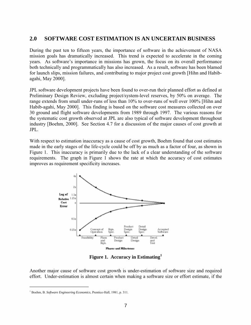
2.0 SOFTWARE COST ESTIMATION IS AN UNCERTAIN BUSINESS During the past ten to fifteen years, the importance of software in the achievement of NASA mission goals has dramatically increased. This trend is expected to accelerate in the coming years. As software�s importance in missions has grown, the focus on its overall performance both technically and programmatically has also increased. As a result, software has been blamed for launch slips, mission failures, and contributing to major project cost growth [Hihn and Habib-agahi, May 2000]. JPL software development projects have been found to over-run their planned effort as defined at Preliminary Design Review, excluding project/system-level reserves, by 50% on average. The range extends from small under-runs of less than 10% to over-runs of well over 100% [Hihn and Habib-agahi, May 2000]. This finding is based on the software cost measures collected on over 30 ground and flight software developments from 1989 through 1997. The various reasons for the systematic cost growth observed at JPL are also typical of software development throughout industry [Boehm, 2000]. See Section 4.7 for a discussion of the major causes of cost growth at JPL. With respect to estimation inaccuracy as a cause of cost growth, Boehm found that cost estimates made in the early stages of the life-cycle could be off by as much as a factor of four, as shown in Figure 1. This inaccuracy is primarily due to the lack of a clear understanding of the software requirements. The graph in Figure 1 shows the rate at which the accuracy of cost estimates improves as requirement specificity increases.

Figure 1. Accuracy in Estimating1

Another major cause of software cost growth is under-estimation of software size and required effort. Under-estimation is almost certain when making a software size or effort estimate, if the

1 Boehm, B. Software Engineering Economics, Prentice-Hall, 1981, p. 311.

8

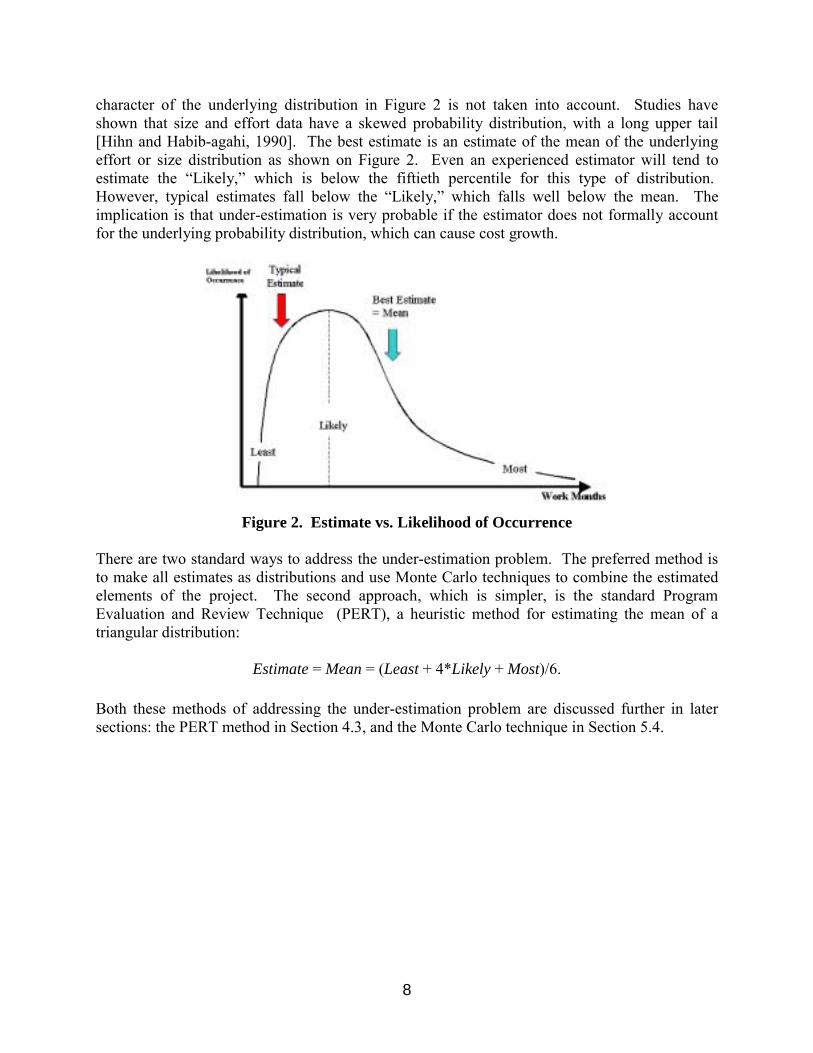
character of the underlying distribution in Figure 2 is not taken into account. Studies have shown that size and effort data have a skewed probability distribution, with a long upper tail [Hihn and Habib-agahi, 1990]. The best estimate is an estimate of the mean of the underlying effort or size distribution as shown on Figure 2. Even an experienced estimator will tend to estimate the �Likely,� which is below the fiftieth percentile for this type of distribution. However, typical estimates fall below the �Likely,� which falls well below the mean. The implication is that under-estimation is very probable if the estimator does not formally account for the underlying probability distribution, which can cause cost growth.

Figure 2. Estimate vs. Likelihood of Occurrence

There are two standard ways to address the under-estimation problem. The preferred method is to make all estimates as distributions and use Monte Carlo techniques to combine the estimated elements of the project. The second approach, which is simpler, is the standard Program Evaluation and Review Technique (PERT), a heuristic method for estimating the mean of a triangular distribution:

Estimate = Mean = (Least + 4*Likely + Most)/6. Both these methods of addressing the under-estimation problem are discussed further in later sections: the PERT method in Section 4.3, and the Monte Carlo technique in Section 5.4.

9

3.0 COST ESTIMATION: APPROACH AND METHODS Cost estimation should never be an activity that is performed independently of technical work. In the early life-cycle phases, cost estimation is closely related to design activities, where the interaction between these activities is iterated many times as part of doing design trade studies and early risk analysis. Later on in the life-cycle, cost estimation supports management activities � primarily detailed planning, scheduling, and risk management.

The purpose of software cost estimation is to:

• Define the resources needed to produce, verify, and validate the software product, and

manage these activities.

• Quantify, insofar as is practical, the uncertainty and risk inherent in this estimate. 3.1 What Should Be Included in the Software Estimate For software development, the dominant cost is the cost of labor. Therefore, it is very important to estimate the software development effort as accurately as possible. A basic cost equation for the costs covered in the handbook can be defined as:

Total_SW_Project$ = SW_Development_Labor$ + Other_Labor$ + Nonlabor$

SW_Development_Labor$ (Steps 2-4, 8) includes: • Software Systems Engineering � performed by the software architect, software system

engineer, and subsystem engineer for functional design, software requirements, and interface specification. Labor for data systems engineering, which is often forgotten, should also be considered. This includes science product definition and data management.

• Software Engineering � performed by the cognizant engineer and developers to unit design, develop code, unit test, and integrate software components

• Software Test Engineering � covers test engineering activities from writing test plans and procedures to performing any level of test above unit testing

Other_Labor$ (Steps 4, 5) includes: • Software management and support � performed by the project element manager (PEM),

software manager, technical lead, and system administration to plan and direct the software project and software configuration management

• Test-bed development • Development Environment Support • Software system-level test support, including development and simulation software • Assembly, Test, & Launch Operations (ATLO) support for flight projects • Administration and Support Costs

10

• Software Quality Assurance • Independent Verification & Validation (IV&V) • Other review or support charges Nonlabor$ (Step 6) includes: • Support and services, such as workstations, test-bed boards & simulators, ground support

equipment, network and phone charges, etc. • Software procurements such as development environment, compilers, licenses, CM tools,

test tools, and development tools • Travel and trips related to customer reviews and interfaces, vendor visits, plus attendance

at project-related conferences • Training

3.2 Estimation Methods All estimates are made based upon some form of analogy: Historical Analogy, Expert Judgment, Models, and �Rules-of-Thumb.� The role these methods play in generating an estimate depends upon where one is in the overall life-cycle. Typically, estimates are made using a combination of these four methods. Model-based estimates along with high-level analogies are the principal source of estimates in early conceptual stages. As a project matures and the requirements and design are better understood, analogy estimates based upon more detailed functional decompositions become the primary method of estimation, with model-based estimates used as a means of estimate validation or as a �sanity-check.�

1. Historical analogy estimation methods are based upon using the software size, effort, or cost of a comparable project from the past. When the term �analogy� is used in this document, it will mean that the comparison is made using measures or data that has been recorded from completed software projects. Analogical estimates can be made at high levels using total software project size and/or cost for individual Work Breakdown Structure (WBS) categories in the process of developing the main software cost estimate. High-level analogies are used for estimate validation or in the very early stages of the life-cycle. Generally, it is necessary to adjust the size or cost of the historical project, as there is rarely a perfect analogy. This is especially true for high-level analogies.

2. Expert judgment estimates are made by the estimator based upon what he or she

remembers it took previous similar projects to complete or how big they were. This is typically a subjective estimate based upon what the estimator remembers from previous projects and gets modified mentally as deemed appropriate. It has been found that expert judgment can be relatively accurate if the estimator has significant recent experience in both the software domain of the planned project, as well as the estimation process itself [Hihn and Habib-agahi, 1990].

11

3. Model-based estimates are estimates made using mathematical relationships or parametric cost models. Parametric cost models are empirical relationships derived by using statistical techniques applied to data from previous projects. . Software cost models provide estimates of effort, cost, and schedule.

4. �Rules-of-thumb� come in a variety of forms and can be a way of expressing estimates as

a simple mathematical relationship (e.g. Effort = Lines_of_Code / 10) or as percentage allocations of effort over activities or phases based upon historical data (e.g. I&T is 22% of Total Effort).

Whatever method is used, it is most important that the assumptions and formulas are documented to enable more thorough review and to make it easier to revise estimates at future dates when assumptions may need to be revised. All four methods are used during the software life-cycle. The level of granularity varies depending on what information is available. At lower-levels of the WBS, expert judgment is the primary method used, while model-based estimates are more common at higher levels of the WBS.

12

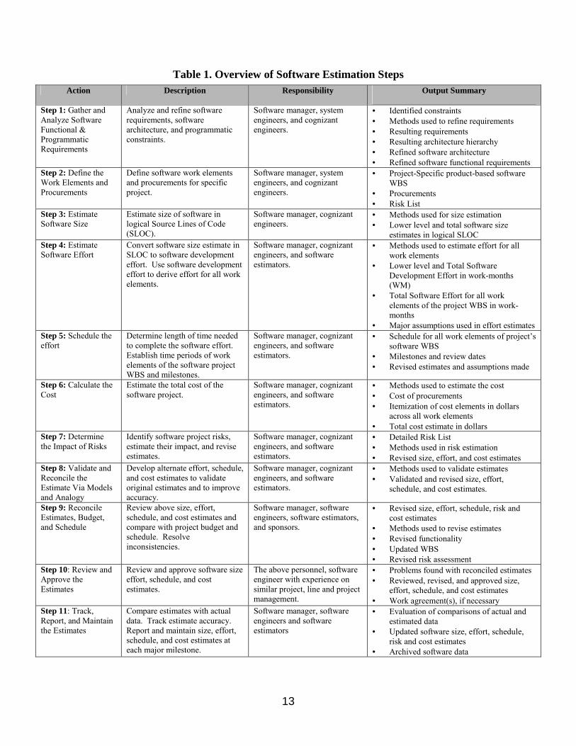
4.0 SOFTWARE ESTIMATION STEPS The cost estimation process includes a number of iterative steps summarized in Table 1. The reason for the iteration over the different steps is that cost estimation is part of the larger planning and design process, in which the system is designed to fit performance, cost, and schedule constraints along with reconciliation and review of the different estimates. Although, in practice, the steps are often performed in a different order and are highly iterative, these steps will be discussed in the sequence that they are numbered for ease of exposition and because this is one of the ideal sequences. For variations in performing the cost estimation steps over the mission life cycle see Appendix C. Software project plans include estimates of cost, product size, resources, staffing levels, schedules, and key milestones. The software estimation process discussed in the following subsections describes the steps for developing software estimates. Establishing this process early in the life-cycle will result in greater accuracy and credibility of estimates and a clearer understanding of the factors that influence software development costs. This process also provides methods for project personnel to identify and monitor cost and schedule risk factors. Table 1 gives a brief description of the software estimation steps. Projects define which personnel are responsible for the activities in the steps. Table 1 presents the roles of personnel who typically perform the activities in each step. The participants should have experience similar to the software under development.

13

Table 1. Overview of Software Estimation Steps

Action Description Responsibility Output Summary

Step 1: Gather and Analyze Software Functional & Programmatic Requirements

Analyze and refine software requirements, software architecture, and programmatic constraints.

Software manager, system engineers, and cognizant engineers.

• Identified constraints • Methods used to refine requirements • Resulting requirements • Resulting architecture hierarchy • Refined software architecture • Refined software functional requirements

Step 2: Define the Work Elements and Procurements

Define software work elements and procurements for specific project.

Software manager, system engineers, and cognizant engineers.

• Project-Specific product-based software WBS

• Procurements • Risk List

Step 3: Estimate Software Size

Estimate size of software in logical Source Lines of Code (SLOC).

Software manager, cognizant engineers.

• Methods used for size estimation • Lower level and total software size

estimates in logical SLOC Step 4: Estimate Software Effort

Convert software size estimate in SLOC to software development effort. Use software development effort to derive effort for all work elements.

Software manager, cognizant engineers, and software estimators.

• Methods used to estimate effort for all work elements

• Lower level and Total Software Development Effort in work-months (WM)

• Total Software Effort for all work elements of the project WBS in work-months

• Major assumptions used in effort estimates Step 5: Schedule the effort

Determine length of time needed to complete the software effort. Establish time periods of work elements of the software project WBS and milestones.


• Schedule for all work elements of project�s software WBS

• Milestones and review dates • Revised estimates and assumptions made

Step 6: Calculate the Cost

Estimate the total cost of the software project.


• Methods used to estimate the cost • Cost of procurements • Itemization of cost elements in dollars

across all work elements • Total cost estimate in dollars

Step 7: Determine the Impact of Risks

Identify software project risks, estimate their impact, and revise estimates.


• Detailed Risk List • Methods used in risk estimation • Revised size, effort, and cost estimates

Step 8: Validate and Reconcile the Estimate Via Models and Analogy

Develop alternate effort, schedule, and cost estimates to validate original estimates and to improve accuracy.


• Methods used to validate estimates • Validated and revised size, effort,

schedule, and cost estimates.

Step 9: Reconcile Estimates, Budget, and Schedule

Review above size, effort, schedule, and cost estimates and compare with project budget and schedule. Resolve inconsistencies.

Software manager, software engineers, software estimators, and sponsors.

• Revised size, effort, schedule, risk and cost estimates

• Methods used to revise estimates • Revised functionality • Updated WBS • Revised risk assessment

Step 10: Review and Approve the Estimates

Review and approve software size effort, schedule, and cost estimates.

The above personnel, software engineer with experience on similar project, line and project management.

• Problems found with reconciled estimates • Reviewed, revised, and approved size,

effort, schedule, and cost estimates • Work agreement(s), if necessary

Step 11: Track, Report, and Maintain the Estimates

Compare estimates with actual data. Track estimate accuracy. Report and maintain size, effort, schedule, and cost estimates at each major milestone.

Software manager, software engineers and software estimators

• Evaluation of comparisons of actual and estimated data

• Updated software size, effort, schedule, risk and cost estimates

• Archived software data

14

4.1 Step 1 - Gather and Analyze Software Functional and Programmatic Requirements

The purpose of this step is to analyze and refine the software functional requirements and to identify technical and programmatic constraints and requirements that will be included in the software estimate. This enables the work elements of the project-specific WBS to be defined and software size and effort to be estimated. Analyze and refine the requirements as follows:

1. Analyze and refine the software functional requirements to the lowest level of detail possible. Clearly identify requirements that are not well understood in order to make appropriate risk adjustments. Unclear requirements are a risk item that should be reflected in greater uncertainty in the software size estimate (to be discussed in Step 3). If an incremental development strategy is used, then the refinement will be based on the requirements that have been defined for each increment.

2. Analyze and refine a software physical architecture hierarchy based on the functional

requirements. Define the architecture in terms of software segments to be developed. Decompose each segment to the lowest level function possible.

3. Analyze project and software plans to identify programmatic constraints and

requirements including imposed budgets, schedules, margins, and make/buy decisions. The outputs of this step are:

• Technical and programmatic constraints and requirements • Assumptions made about the constraints and requirements • Methods used to refine the software functional requirements • Refined software functional requirements • Software architecture hierarchy of segments and associated functions

4.2 Step 2 - Define the Work Elements and Procurements The purpose of this step is to define the work elements and procurements for the software project that will be included in the software estimate.

1. Use the WBS in Appendix D of this document as a starting point to plan the work elements and procurements for the project that requires estimation. Then consult your project-specific WBS to find additional applicable work elements.

The work elements and procurements will typically fall into the following categories of a project-specific WBS:

• Software Management • Software Systems Engineering • Software Engineering

15

• Software Test Engineering • Software Development Test Bed • Software Development Environment • Software System-level Test Support • Assembly, Test, Launch Operations (ATLO) Support for flight projects • SQA • IV&V

These WBS categories include activities across the software life-cycle from requirements analysis through completion of system test. Note that software operations and support (including maintenance) is not in the scope of these estimates. Work elements such as SQA and IV&V are not often part of the software manager�s budget, but are listed here to remind software managers that these services are being provided by the project.

2. Identify the attributes of the work elements that will drive the size and effort estimates in

terms of heritage and risk. From this, derive an initial risk list. Examples2 are: • Anything that is new, such as code, language, or design method • Low technology readiness levels • Overly optimistic assumptions related to high heritage elements • Possible reuse • Vendor-related risks associated with Commercial Off-The-Shelf (COTS) software • Criticality of mission failure • Software classification • Use of development tools • Concurrent development of hardware • Number of interfaces between multiple development organizations • Geographical distribution of multiple development organizations • High complexity elements • Skill and experience level of team • Vague or incomplete requirements

The outputs of this step include the following: • Assumptions about the work elements and procurements • List of procurements • Project-specific product-based software WBS including attributes of the work elements • Risk List

4.3 Step 3 - Estimate Software Size The purpose of this step is to estimate the size of the software product. Because formal cost estimation techniques require software size as an input [Parametric Estimation Handbook, 1999 and NASA Cost Estimation Handbook, 2002], size prediction is essential to effective effort

2 For a more comprehensive list of attributes that drive size and effort, see Boehm, et al. 2000.

16

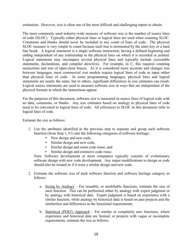
estimation. However, size is often one of the most difficult and challenging inputs to obtain. The most commonly used industry-wide measure of software size is the number of source lines of code (SLOC). Typically either physical lines or logical lines are used when counting SLOC. Comments and blanks should never be included in any count of lines of code. The physical SLOC measure is very simple to count because each line is terminated by the enter key or a hard line break. A logical statement is a single software instruction, having a defined beginning and ending independent of any relationship to the physical lines on which it is recorded or printed. Logical statements may encompass several physical lines and typically include executable statements, declarations, and compiler directives. For example, in C, this requires counting semicolons and sets of open-close braces. As it is considered more accurate and changes less between languages, most commercial cost models require logical lines of code as input rather than physical lines of code. In some programming languages, physical lines and logical statements are nearly the same, but in others, significant differences in size estimates can result. Logical source statements are used to measure software size in ways that are independent of the physical formats in which the instructions appear. For the purposes of this document, software size is measured in source lines of logical code with no data, comments, or blanks. Any size estimates based on analogy to physical lines of code need to be converted to logical lines of code. All references to SLOC in this document refer to logical lines of code. Estimate the size as follows:

1. Use the attributes identified in the previous step to separate and group each software function (from Step 1, #1) into the following categories of software heritage:

• New design and new code, • Similar design and new code, • Similar design and some code reuse, and • Similar design and extensive code reuse.

Note: Software development at most companies typically consists of evolutionary software design with new code development. Any major modifications to design or code should also be treated as if it were a similar design and new code.

2. Estimate the software size of each software function and software heritage category as

follows:

a. Sizing by Analogy � For reusable, or modifiable functions, estimate the size of each function. This can be performed either by analogy with expert judgment or by analogy with historical data. Expert judgment is based on experience with a similar function, while analogy by historical data is based on past projects and the similarities and differences in the functional requirements.

b. Statistical (PERT) Approach � For similar or completely new functions, where

experience and historical data are limited, or projects with vague or incomplete requirements, estimate the size as follows:

17

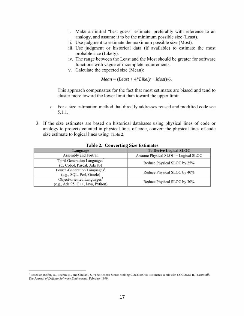
i. Make an initial �best guess� estimate, preferably with reference to an analogy, and assume it to be the minimum possible size (Least).

ii. Use judgment to estimate the maximum possible size (Most). iii. Use judgment or historical data (if available) to estimate the most

probable size (Likely). iv. The range between the Least and the Most should be greater for software

functions with vague or incomplete requirements. v. Calculate the expected size (Mean):

Mean = (Least + 4*Likely + Most)/6.

This approach compensates for the fact that most estimates are biased and tend to cluster more toward the lower limit than toward the upper limit.

c. For a size estimation method that directly addresses reused and modified code see

5.1.1.

3. If the size estimates are based on historical databases using physical lines of code or analogy to projects counted in physical lines of code, convert the physical lines of code size estimate to logical lines using Table 2.

Table 2. Converting Size Estimates

Language To Derive Logical SLOC Assembly and Fortran Assume Physical SLOC = Logical SLOC

Third-Generation Languages3

(C, Cobol, Pascal, Ada 83) Reduce Physical SLOC by 25%

Fourth-Generation Languages3 (e.g., SQL, Perl, Oracle) Reduce Physical SLOC by 40%

Object-oriented Languages3

(e.g., Ada 95, C++, Java, Python) Reduce Physical SLOC by 30%

3 Based on Reifer, D., Boehm, B., and Chulani, S. �The Rosetta Stone: Making COCOMO 81 Estimates Work with COCOMO II,� Crosstalk: The Journal of Defense Software Engineering, February 1999.

18

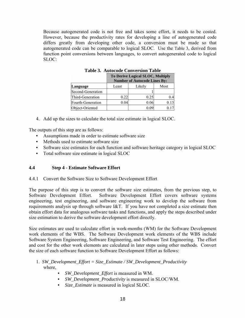
Because autogenerated code is not free and takes some effort, it needs to be costed. However, because the productivity rates for developing a line of autogenerated code differs greatly from developing other code, a conversion must be made so that autogenerated code can be comparable to logical SLOC. Use the Table 3, derived from function point conversions between languages, to convert autogenerated code to logical SLOC:

Table 3. Autocode Conversion Table

To Derive Logical SLOC, Multiply

Number of Autocode Lines By: Language Least Likely Most Second-Generation 1 Third-Generation 0.22 0.25 0.4 Fourth-Generation 0.04 0.06 0.13 Object-Oriented 0.09 0.17

4. Add up the sizes to calculate the total size estimate in logical SLOC.

The outputs of this step are as follows:

• Assumptions made in order to estimate software size • Methods used to estimate software size • Software size estimates for each function and software heritage category in logical SLOC • Total software size estimate in logical SLOC

4.4 Step 4 - Estimate Software Effort 4.4.1 Convert the Software Size to Software Development Effort The purpose of this step is to convert the software size estimates, from the previous step, to Software Development Effort. Software Development Effort covers software systems engineering, test engineering, and software engineering work to develop the software from requirements analysis up through software I&T. If you have not completed a size estimate then obtain effort data for analogous software tasks and functions, and apply the steps described under size estimation to derive the software development effort directly. Size estimates are used to calculate effort in work-months (WM) for the Software Development work elements of the WBS. The Software Development work elements of the WBS include Software System Engineering, Software Engineering, and Software Test Engineering. The effort and cost for the other work elements are calculated in later steps using other methods. Convert the size of each software function to Software Development Effort as follows:

1. SW_Development_Effort = Size_Estimate / SW_Development_Productivity

where, • SW_Development_Effort is measured in WM. • SW_Development_Productivity is measured in SLOC/WM. • Size_Estimate is measured in logical SLOC.

19

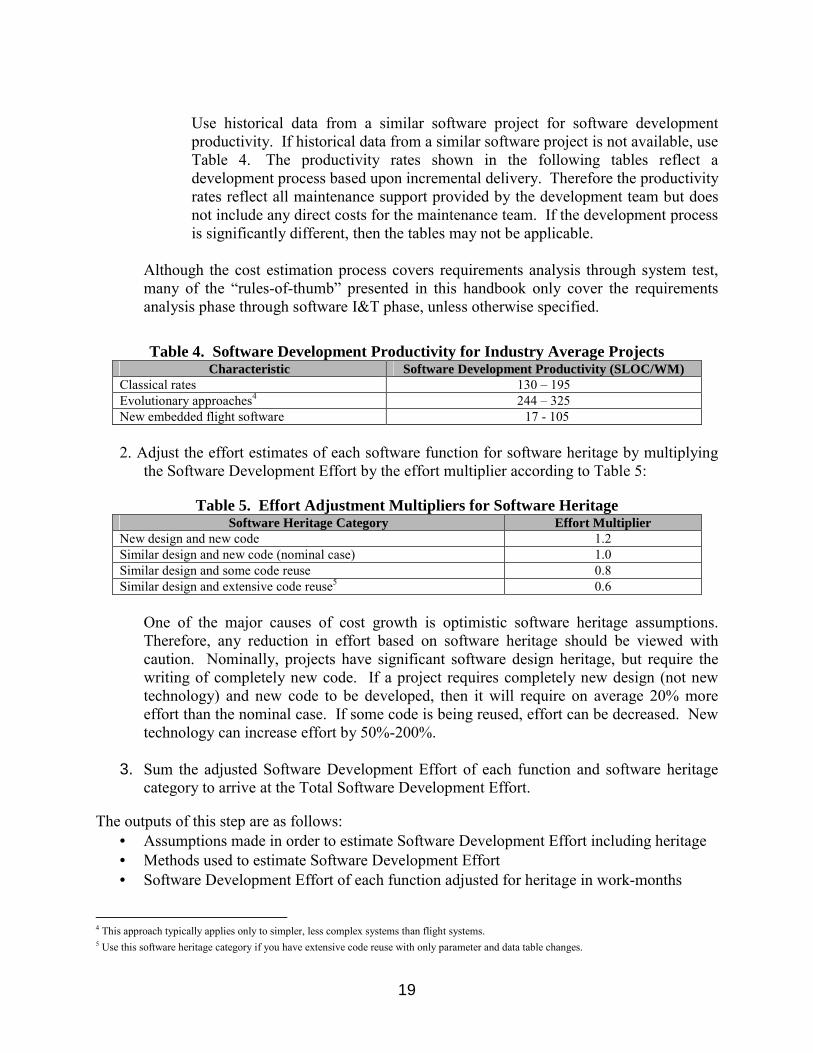
Use historical data from a similar software project for software development productivity. If historical data from a similar software project is not available, use Table 4. The productivity rates shown in the following tables reflect a development process based upon incremental delivery. Therefore the productivity rates reflect all maintenance support provided by the development team but does not include any direct costs for the maintenance team. If the development process is significantly different, then the tables may not be applicable.

Although the cost estimation process covers requirements analysis through system test, many of the �rules-of-thumb� presented in this handbook only cover the requirements analysis phase through software I&T phase, unless otherwise specified.

Table 4. Software Development Productivity for Industry Average Projects Characteristic Software Development Productivity (SLOC/WM)

Classical rates 130 � 195 Evolutionary approaches4 244 � 325 New embedded flight software 17 - 105

2. Adjust the effort estimates of each software function for software heritage by multiplying

the Software Development Effort by the effort multiplier according to Table 5:

Table 5. Effort Adjustment Multipliers for Software Heritage Software Heritage Category Effort Multiplier

New design and new code 1.2 Similar design and new code (nominal case) 1.0 Similar design and some code reuse 0.8 Similar design and extensive code reuse5 0.6

One of the major causes of cost growth is optimistic software heritage assumptions. Therefore, any reduction in effort based on software heritage should be viewed with caution. Nominally, projects have significant software design heritage, but require the writing of completely new code. If a project requires completely new design (not new technology) and new code to be developed, then it will require on average 20% more effort than the nominal case. If some code is being reused, effort can be decreased. New technology can increase effort by 50%-200%.

3. Sum the adjusted Software Development Effort of each function and software heritage category to arrive at the Total Software Development Effort.


• Assumptions made in order to estimate Software Development Effort including heritage • Methods used to estimate Software Development Effort • Software Development Effort of each function adjusted for heritage in work-months

4 This approach typically applies only to simpler, less complex systems than flight systems. 5 Use this software heritage category if you have extensive code reuse with only parameter and data table changes.

20

• Total Software Development Effort in work-months 4.4.2 Extrapolate and Complete the Effort Estimate The purpose of this step is to extend the estimates to cover all work elements of the WBS. Up to this step, the estimates have only covered the Software Development (activities associated with Software System Engineering, Software Engineering, and Software Test Engineering) work elements of the WBS. Effort such as Software Management effort and Software Quality Assurance Effort, are in addition to the Software Development Effort.

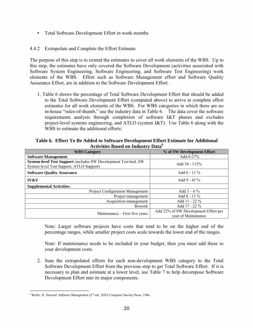
1. Table 6 shows the percentage of Total Software Development Effort that should be added to the Total Software Development Effort (computed above) to arrive at complete effort estimates for all work elements of the WBS. For WBS categories in which there are no in-house �rules-of-thumb,� use the industry data in Table 6. The data cover the software requirements analysis through completion of software I&T phases and excludes project-level systems engineering, and ATLO (system I&T). Use Table 6 along with the WBS to estimate the additional efforts:

Table 6. Effort To Be Added to Software Development Effort Estimate for Additional Activities Based on Industry Data6

WBS Category % of SW Development Effort Software Management Add 6-27% System-level Test Support (includes SW Development Test-bed, SW System-level Test Support, ATLO Support) Add 34 - 112%

Software Quality Assurance Add 6 - 11 %

IV&V Add 9 - 45 % Supplemental Activities:

Project Configuration Management Add 3 � 6 % Project management Add 8 - 11 %

Acquisition management Add 11 - 22 % Rework Add 17 - 22 %

Maintenance � First five years Add 22% of SW Development Effort per year of Maintenance

Note: Larger software projects have costs that tend to be on the higher end of the percentage ranges, while smaller project costs scale towards the lower end of the ranges. Note: If maintenance needs to be included in your budget, then you must add these to your development costs.

2. Sum the extrapolated efforts for each non-development WBS category to the Total

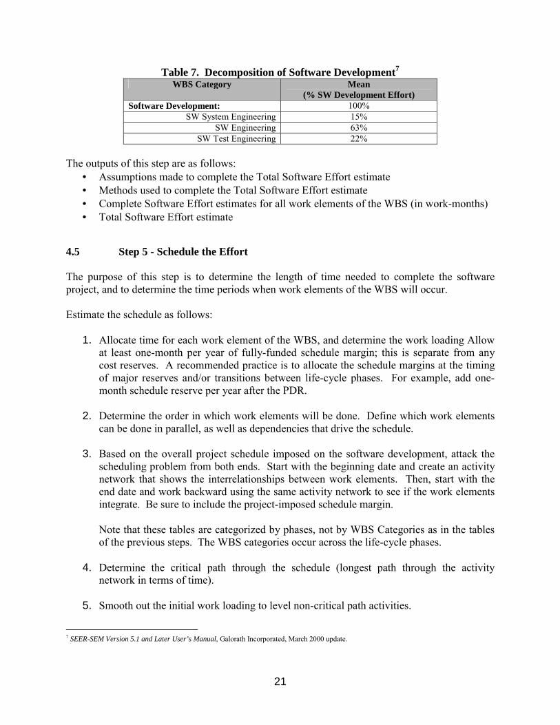
Software Development Effort from the previous step to get Total Software Effort. If it is necessary to plan and estimate at a lower level, use Table 7 to help decompose Software Development Effort into its major components.

6 Reifer, D. Tutorial: Software Management (3rd ed). IEEE Computer Society Press: 1986.

21

Table 7. Decomposition of Software Development7

WBS Category Mean (% SW Development Effort)

Software Development: 100% SW System Engineering 15%

SW Engineering 63% SW Test Engineering 22%


• Assumptions made to complete the Total Software Effort estimate • Methods used to complete the Total Software Effort estimate • Complete Software Effort estimates for all work elements of the WBS (in work-months) • Total Software Effort estimate

4.5 Step 5 - Schedule the Effort The purpose of this step is to determine the length of time needed to complete the software project, and to determine the time periods when work elements of the WBS will occur. Estimate the schedule as follows:

1. Allocate time for each work element of the WBS, and determine the work loading Allow at least one-month per year of fully-funded schedule margin; this is separate from any cost reserves. A recommended practice is to allocate the schedule margins at the timing of major reserves and/or transitions between life-cycle phases. For example, add one-month schedule reserve per year after the PDR.

2. Determine the order in which work elements will be done. Define which work elements

can be done in parallel, as well as dependencies that drive the schedule.

3. Based on the overall project schedule imposed on the software development, attack the scheduling problem from both ends. Start with the beginning date and create an activity network that shows the interrelationships between work elements. Then, start with the end date and work backward using the same activity network to see if the work elements integrate. Be sure to include the project-imposed schedule margin.

Note that these tables are categorized by phases, not by WBS Categories as in the tables of the previous steps. The WBS categories occur across the life-cycle phases.

4. Determine the critical path through the schedule (longest path through the activity

network in terms of time).

5. Smooth out the initial work loading to level non-critical path activities.

7 SEER-SEM Version 5.1 and Later User’s Manual, Galorath Incorporated, March 2000 update.

22

6. Inconsistencies and holes in the estimates may appear while scheduling the individual

work elements and determining resource loading. This is especially true when trying to fit the work elements into the schedule imposed on the software project. As a result, it may be necessary to reiterate the estimates of other steps several times, to reduce the effort, or assume more risk to fit into the imposed schedule. See later steps for reviewing estimates versus budgets and schedule.

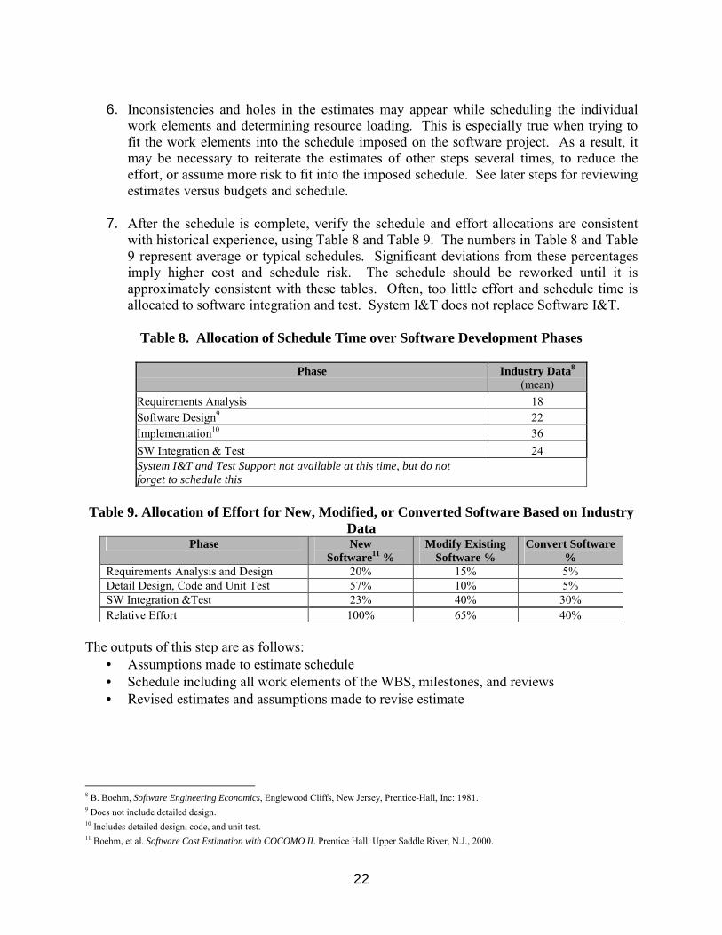
7. After the schedule is complete, verify the schedule and effort allocations are consistent

with historical experience, using Table 8 and Table 9. The numbers in Table 8 and Table 9 represent average or typical schedules. Significant deviations from these percentages imply higher cost and schedule risk. The schedule should be reworked until it is approximately consistent with these tables. Often, too little effort and schedule time is allocated to software integration and test. System I&T does not replace Software I&T.

Table 8. Allocation of Schedule Time over Software Development Phases

Phase

Industry Data8

(mean) Requirements Analysis 18 Software Design9 22 Implementation10 36 SW Integration & Test 24 System I&T and Test Support not available at this time, but do not forget to schedule this

Table 9. Allocation of Effort for New, Modified, or Converted Software Based on Industry

Data Phase New

Software11 % Modify Existing

Software % Convert Software

% Requirements Analysis and Design 20% 15% 5% Detail Design, Code and Unit Test 57% 10% 5% SW Integration &Test 23% 40% 30% Relative Effort 100% 65% 40%


• Assumptions made to estimate schedule • Schedule including all work elements of the WBS, milestones, and reviews • Revised estimates and assumptions made to revise estimate

8 B. Boehm, Software Engineering Economics, Englewood Cliffs, New Jersey, Prentice-Hall, Inc: 1981. 9 Does not include detailed design. 10 Includes detailed design, code, and unit test. 11 Boehm, et al. Software Cost Estimation with COCOMO II. Prentice Hall, Upper Saddle River, N.J., 2000.

23

4.6 Step 6 - Calculate the Cost The purpose of this step is to estimate the total cost of the software project to cover the work elements and procurements of the WBS. Estimate the total cost as follows:

1. Determine the cost of procurements:

a. Determine the cost of support and services, such as workstations, test-bed boards and simulators, ground support equipment, and network and phone charges.

b. Determine the cost of software procurements such as operating systems,

compilers, licenses, and development tools.

c. Determine the cost of travel and trips related to customer reviews and interfaces, vendor visits, plus attendance at project-related conferences.

2. Determine the cost of training planned for the software project. 3. Determine the salary and skill level of the labor force.

4. Input the effort, salary levels, and cost of procurements into an institutionally supported

budgeting tool to determine overall cost. All estimates should be integrated with all rates and factors, institutional standard inflation rates, and median salaries.

5. As with scheduling, inconsistencies and holes in the estimates may appear while

calculating the cost. This is especially true when trying to fit the cost into the budget imposed on the software project. As a result, it may be necessary to reiterate the estimates of other steps several times, reduce the effort and procurements, or assume more risk to fit into the imposed budget. If the schedule becomes extended, costs will rise because effort moves out to more expensive years. See later steps for reviewing estimates versus budgets and schedule.


• Assumptions made to estimate cost • Methods used to estimate cost • Cost of procurements • Itemized cost estimates by WBS elements (in dollars) • Total cost estimate (in dollars)

24

4.7 Step 7 - Determine the Impact of Risks The purpose of this step is to identify the software project risks, to assess their impact on the cost estimate, and to revise the estimates based on the impacts. Assess the risks as follows:

1. Take the initial risk list from Step 2, and identify the major risks that present the greatest impact and uncertainty to the software estimates.

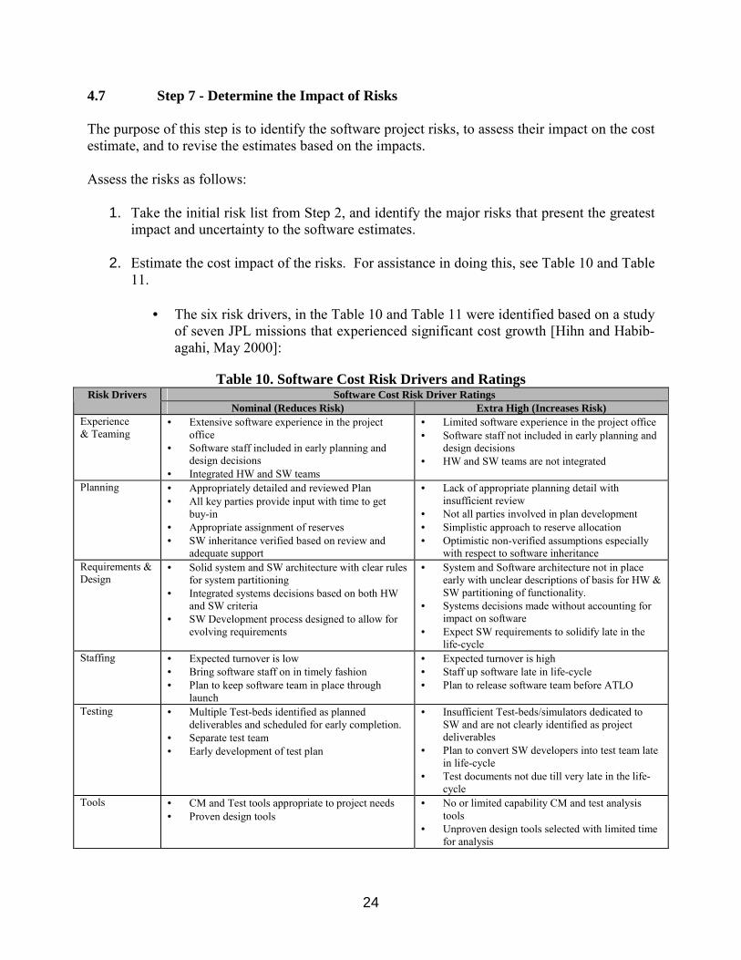
2. Estimate the cost impact of the risks. For assistance in doing this, see Table 10 and Table

11.

• The six risk drivers, in the Table 10 and Table 11 were identified based on a study of seven JPL missions that experienced significant cost growth [Hihn and Habib-agahi, May 2000]:

Table 10. Software Cost Risk Drivers and Ratings Software Cost Risk Driver Ratings Risk Drivers

Nominal (Reduces Risk) Extra High (Increases Risk) Experience & Teaming

• Extensive software experience in the project office

• Software staff included in early planning and design decisions

• Integrated HW and SW teams

• Limited software experience in the project office • Software staff not included in early planning and

design decisions • HW and SW teams are not integrated

Planning • Appropriately detailed and reviewed Plan • All key parties provide input with time to get

buy-in • Appropriate assignment of reserves • SW inheritance verified based on review and

adequate support

• Lack of appropriate planning detail with insufficient review

• Not all parties involved in plan development • Simplistic approach to reserve allocation • Optimistic non-verified assumptions especially

with respect to software inheritance Requirements & Design

• Solid system and SW architecture with clear rules for system partitioning

• Integrated systems decisions based on both HW and SW criteria

• SW Development process designed to allow for evolving requirements

• System and Software architecture not in place early with unclear descriptions of basis for HW & SW partitioning of functionality.

• Systems decisions made without accounting for impact on software

• Expect SW requirements to solidify late in the life-cycle

Staffing • Expected turnover is low • Bring software staff on in timely fashion • Plan to keep software team in place through

launch

• Expected turnover is high • Staff up software late in life-cycle • Plan to release software team before ATLO

Testing • Multiple Test-beds identified as planned deliverables and scheduled for early completion.

• Separate test team • Early development of test plan

• Insufficient Test-beds/simulators dedicated to SW and are not clearly identified as project deliverables

• Plan to convert SW developers into test team late in life-cycle

• Test documents not due till very late in the life-cycle

Tools • CM and Test tools appropriate to project needs • Proven design tools

• No or limited capability CM and test analysis tools

• Unproven design tools selected with limited time for analysis

25

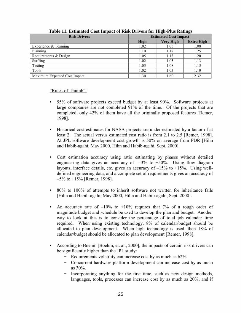
Table 11. Estimated Cost Impact of Risk Drivers for High-Plus Ratings Estimated Cost Impact Risk Drivers

High Very High Extra High Experience & Teaming 1.02 1.05 1.08 Planning 1.10 1.17 1.25 Requirements & Design 1.05 1.13 1.20 Staffing 1.02 1.05 1.13 Testing 1.05 1.08 1.15 Tools 1.02 1.03 1.10 Maximum Expected Cost Impact 1.30 1.60 2.32

�Rules-of-Thumb�: • 55% of software projects exceed budget by at least 90%. Software projects at

large companies are not completed 91% of the time. Of the projects that are completed, only 42% of them have all the originally proposed features [Remer, 1998].

• Historical cost estimates for NASA projects are under-estimated by a factor of at

least 2. The actual versus estimated cost ratio is from 2.1 to 2.5 [Remer, 1998]. At JPL software development cost growth is 50% on average from PDR [Hihn and Habib-agahi, May 2000, Hihn and Habib-agahi, Sept. 2000]

• Cost estimation accuracy using ratio estimating by phases without detailed

engineering data gives an accuracy of �3% to +50%. Using flow diagram layouts, interface details, etc. gives an accuracy of �15% to +15%. Using well-defined engineering data, and a complete set of requirements gives an accuracy of �5% to +15% [Remer, 1998].

• 80% to 100% of attempts to inherit software not written for inheritance fails

[Hihn and Habib-agahi, May 2000, Hihn and Habib-agahi, Sept. 2000]. • An accuracy rate of �10% to +10% requires that 7% of a rough order of

magnitude budget and schedule be used to develop the plan and budget. Another way to look at this is to consider the percentage of total job calendar time required. When using existing technology, 8% of calendar/budget should be allocated to plan development. When high technology is used, then 18% of calendar/budget should be allocated to plan development [Remer, 1998].

• According to Boehm [Boehm, et. al., 2000], the impacts of certain risk drivers can

be significantly higher than the JPL study: − Requirements volatility can increase cost by as much as 62%. − Concurrent hardware platform development can increase cost by as much

as 30%. − Incorporating anything for the first time, such as new design methods,

languages, tools, processes can increase cost by as much as 20%, and if

26

there are multiple sources of newness, it can increase cost as much as 100%.

3. Estimate Risk Adjustment factor in one of the following ways:

a. Simple Risk Adjustment: Adjust the cost estimate to reflect the impact of risk. It is assumed that each risk independently increases cost. Multiply expected cost impacts together to combine and get a total impact factor. (Subtracting 1.0 from the total impact gives the total percentage impact.) Adjust the cost estimate by multiplying by the total risk adjustment factor. See Appendix F, Step 7, for an example calculation of risk.

b. Expert Risk Adjustment: Estimate the likelihood of occurrence based on expert

judgment for each risk and its impact. Derive the expected value of the risk as follows:

∑=

n

i 1

[(Impacti)*(Likelihood_of_Occurrencei)]

Adjust the cost estimate by adding the total risk adjustment factor to the cost.

4. Adjust any other estimates based on the risk assessment.

5. Update the risk assessment each time the software estimates are updated. This increased cost estimate can be used to negotiate the use of budgetary reserves.


• Detailed software project risk list • Assumptions made to revise estimates • Methods used to revise estimates • Revised size, effort, schedule, and cost estimates for risk

4.8 Step 8 - Validate and Reconcile the Estimate via Models and Analogy The purpose of this step is to validate the estimates.

1. In addition to the main estimate that was developed in the preceding steps, obtain a second estimate, using one of the following:

a. Alternate Estimate

Have a second person or team, with similar software experience, generate independent estimates.

b. Historical Analogies

Using historical data, compare the estimates with previous experience such as in the following areas:

27

• Size, effort, and cost of similar software • Size versus functions • Size versus effort and cost (development productivity) • Technology versus effort and cost

c. Model-Based Estimates

See Section 5 for discussion on performing a model-based estimate.

2. Have the responsible people for this step meet to compare the main estimates with the second

estimates, resolve the differences, and refine the estimates until a consensus estimate is reached. The lowest estimates should be given special scrutiny, as experience has demonstrated that estimates are usually low. For specific information on validating and reconciling estimates with models, see Section 5.5.


• Assumptions made to validate the estimates • Methods used to validate the estimates • Validated and revised size, effort, schedule, and cost estimates with improved

accuracy 4.9 Step 9 - Reconcile Estimates, Budget, and Schedule The purpose of this step is to review the validated estimates with respect to the project-imposed budget and schedule and to resolve the differences. In many ways, Steps 9 and 10 are the most difficult steps in the cost estimation process, because of the need to understand, in an integrated manner, the cost of individual functions, their relative prioritization, and the functional interrelationships. If an inconsistency arises, there is a tendency to incorrectly address the issue as only a problem of incorrect estimation. However, in most cases, the real solution is to descope or reduce functionality, and then to descope again, until the task fits the budget. Do not reduce costs by eliminating reserves and making optimistic and unrealistic assumptions. 1. Calculate the budget margin. Subtract the estimated cost from the budgeted cost. Then

divide by the budgeted cost to get the margins. Multiply by 100 to get percent margin. Calculate schedule margin in the same manner.

2. Compare the estimated cost, schedule, and margins to the project-imposed budget, schedule, and margins to determine if they are consistent.

3. If the estimates are substantially greater, then identify and resolve the differences:

a. Refine the desired scope and functionality to the lowest level possible by analyzing and prioritizing the functions to identify those functions that can be eliminated. Make certain you account for interrelationships between functions.

b. Begin eliminating procurements that are not absolutely necessary.

28

c. Revise the schedule, cost estimates, and risks to reflect the reductions in cost based on

steps a-d. Reducing high-risk functionality or procurements can reduce risk and costs greatly.

d. Repeat the process until the functionality and procurements are affordable, with

respect to the budget, and feasible, with respect to the imposed schedule. e. Review the reduced functionality, reduced procurements, and the corresponding

revised estimates with the sponsor to reach agreement. If agreement cannot be reached, higher-level management may need to intervene and assume a greater risk to maintain functionality. Update the WBS according to the revised functionality.

f. As the project progresses, it may be possible to include some functions or

procurements that were originally not thought to be affordable or feasible. The outputs of this step are as follows:

• Assumptions made to revise estimates • Methods used to revise estimates • Revised size, effort, schedule, and cost estimates • Revised functionality and procurements • Updated WBS • Revised risk assessment

4.10 Step 10 - Review and Approve the Estimates The purpose of this step is to review the software estimates and to obtain project and line management approval.

1. Conduct a peer review with the following objectives: • Confirm the WBS and the software architecture. • Verify the methods used for deriving the size, effort, schedule, and cost. Signed work

agreements may be necessary. • Ensure the assumptions and input data used to develop the estimates are correct. • Ensure that the estimates are reasonable and accurate, given the input data. • Formally confirm and record the approved software estimates and underlying

assumptions for the project.

2. The software manager, software estimators, line management, and project management approve the software estimates after the review is complete and problems have been resolved. Remember that costs cannot be reduced without reducing functionality.


• Problems found with the estimates • Reviewed, revised, and approved size, effort, schedule, cost estimates, and assumptions

29

• Work Agreement(s), if necessary

4.11 Step 11 - Track, Report, and Maintain the Estimates The purpose of this step is to check the accuracy of the software estimates over time, and provide the estimates to save for use in future software project estimates.

1. Track the estimates to identify when, how much, and why the project may be over-running or under-running the estimates. Compare current estimates, and ultimately actual data, with past estimates and budgets to determine the variation of the estimates over time. This allows estimators to see how well they are estimating and how the software project is changing over time.

2. Document changes between the current and past estimates and budgets.

3. In order to improve estimation and planning, archive software estimation and actual data

each time an estimate is updated and approved, usually at each major milestone. It is recommended that the following data be archived:

• Project contextual and supporting information

− Project name − Software organization − Platform − Language − Estimation method(s) and assumptions − Date(s) of approved estimate(s)

• Estimated and actual size, effort, cost, and cost of procurements by WBS work element

• Planned and actual schedule dates of major milestones and reviews • Identified risks and their estimated and actual impacts


• Updated tracking comparisons of actual and estimated data • Evaluation of the comparisons • Updated size, effort, schedule, cost estimates, and risk assessment • Archived software data, including estimates and actuals

30

5.0 PARAMETRIC SOFTWARE COST ESTIMATION Parametric or model-based cost estimates can be used as a primary estimate or as a secondary backup estimate for validation, depending upon where in the life-cycle the project is. As a project matures and the requirements and design are better understood, analogy estimates based upon more detailed functional decompositions should be the primary method of estimation, with model-based estimates used as a means of validation. However, in the early stages of the software life-cycle, when requirements and design are still vague, model-based estimates, along with high-level analogies, are the principal source of estimates. In addition, model-based estimates can help you �reason about the cost and schedule implications of software decisions� [Boehm, 1981]. Model-based estimates can also be used to understand tradeoffs by analyzing the relative impacts of different development scenarios. Before using a cost estimation model in your organization it is strongly recommend that it be validated and, if possible, calibrated to your environment. The Post-Architecture COCOMO II Model, SEER-SEM, and Price S have been assessed �out of the box� with no calibration, for JPL usage, and they predict software costs reasonably well in the JPL environment. See [Lum, Powell, Hihn, 2002] for the results and description of how to validate a cost model. 5.1 Model Structure Many parametric models compute effort in a similar manner, where estimated effort is proportional to size raised to a factor:

E = [A (Size)B (EM)] where

E is estimated effort in work-months. A is a constant that reflects a measure of the basic organizational/ technology costs. Size is the equivalent number of new logical lines of code. Equivalent lines are the new

lines of code and the new lines of adapted code. Equivalent lines of code takes into account the additional effort required to modify reused/adapted code for inclusion into the software product. Most parametric tools automatically compute the equivalent lines of code from size and heritage percentage inputs. Size also takes into consideration any code growth from requirements evolution/volatility.

B is a scaling factor of size. It is a variable exponent whose values represent economies/diseconomies of scale.

EM is the product of a group of effort multipliers that measure environmental factors used to adjust effort (E). The set of factors comprising EM are commonly referred to as cost drivers because they adjust the final effort estimate up or down.

The effort algorithm is of a multiplicative form. This means that the margins for error in the estimates are expressed as a percentage. Therefore, large projects will have a larger variance in dollars than smaller projects. COCOMO II equations are explained in detail in [Boehm, et al., 2000]. Parameter (input) sensitivities and other insights into the model are also found in the user's documentation.

31

5.2 USC COCOCOMO II Because it is an open book model, COCOMO II will be used as the example for performing a model-based estimate in the remainder of this chapter. USC COCOMO II is a tool developed by the Center for Software Engineering (CSE) at the University of Southern California (USC), headed by Dr. Barry Boehm. Unlike other cost estimation models, COCOMO II is an open model, so all of the details are published. There are different versions of the model � one for early software design phases (the Early Design Model) and one for later software development phases (the Post-Architecture Model). The amount of information available during the different phases of software development varies, and COCOMO II incorporates this by requiring fewer cost drivers during the early design phase of development versus the post-architecture phases. This tool allows for estimation by modules and distinguishes between new development and reused/adapted software. This chapter of the handbook is intended as a basic introduction to COCOMO II. In addition, to this handbook, training may be needed to use the tool effectively. For additional help, the following document provides detailed information about the model/tool:

• B. Boehm, et al., Software Cost Estimation with COCOMO II, Upper Saddle

River, New Jersey, Prentice Hall PTR: 2000.

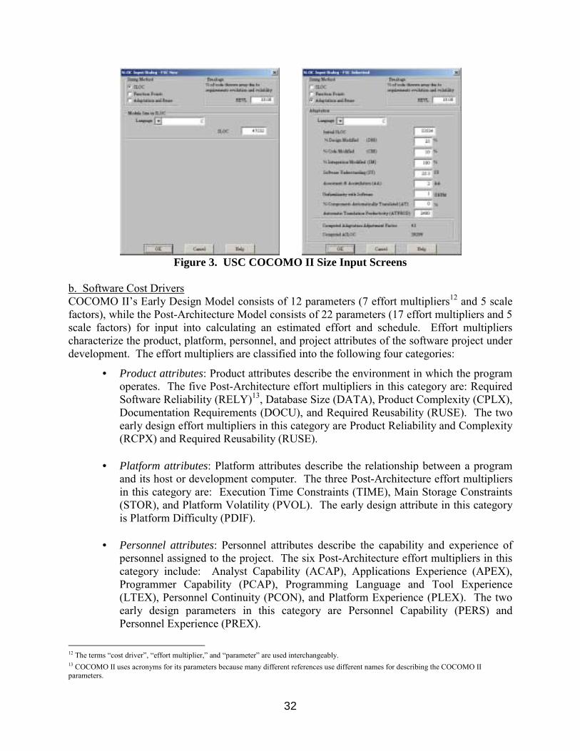
5.2.1 Inputs a. Software Size Software size is the primary parameter in most cost estimation models and formal cost estimation techniques. Size data can be entered in USC COCOMO II either as logical source lines of code or as function points (a measure of the amount of functionality contained in a given piece of software that quantifies the information processing functionality associated with major external data input, output, and/or file types). More information on function points can be obtained from the International Function Point Users Group at http://ifpug.org.

1. Take the logical lines of code size estimates for each software function from Software Estimation Step #3 (Section 4.3) as the first inputs into the tool.

2. If there is reuse or inheritance, enter the number of SLOC to be inherited or reused.

Enter the percentages of design modification, code modification, and additional integration and testing required of the inherited software (Figure 3). From these numbers, the tools derive an equivalent size, since inheritance and reuse are not free and contribute to the software product�s effective size.

32

Figure 3. USC COCOMO II Size Input Screens

b. Software Cost Drivers COCOMO II�s Early Design Model consists of 12 parameters (7 effort multipliers12 and 5 scale factors), while the Post-Architecture Model consists of 22 parameters (17 effort multipliers and 5 scale factors) for input into calculating an estimated effort and schedule. Effort multipliers characterize the product, platform, personnel, and project attributes of the software project under development. The effort multipliers are classified into the following four categories:

• Product attributes: Product attributes describe the environment in which the program operates. The five Post-Architecture effort multipliers in this category are: Required Software Reliability (RELY)13, Database Size (DATA), Product Complexity (CPLX), Documentation Requirements (DOCU), and Required Reusability (RUSE). The two early design effort multipliers in this category are Product Reliability and Complexity (RCPX) and Required Reusability (RUSE).

• Platform attributes: Platform attributes describe the relationship between a program

and its host or development computer. The three Post-Architecture effort multipliers in this category are: Execution Time Constraints (TIME), Main Storage Constraints (STOR), and Platform Volatility (PVOL). The early design attribute in this category is Platform Difficulty (PDIF).

• Personnel attributes: Personnel attributes describe the capability and experience of

personnel assigned to the project. The six Post-Architecture effort multipliers in this category include: Analyst Capability (ACAP), Applications Experience (APEX), Programmer Capability (PCAP), Programming Language and Tool Experience (LTEX), Personnel Continuity (PCON), and Platform Experience (PLEX). The two early design parameters in this category are Personnel Capability (PERS) and Personnel Experience (PREX).

12 The terms �cost driver�, �effort multiplier,� and �parameter� are used interchangeably. 13 COCOMO II uses acronyms for its parameters because many different references use different names for describing the COCOMO II parameters.

33

• Project attributes: Project attributes describe selected project management facets of a

program. The three Post-Architecture effort multipliers in this category include: Use of Software Tools (TOOL), Multiple Site Development (SITE), and Required Development Schedule (SCED). The two early design effort multipliers in this category are Required Development Schedule (SCED) and Facilities (FCIL).

• Scale factors capture features of a software project that can account for relative

economies or diseconomies of scale. Economies of scale means that doubling the size would less than double the cost. Diseconomies of scale means doubling the size would more than double the cost. The five scale factors are Precedentedness (PREC), Flexibility (FLEX), Architecture and Risk Resolution (RESL), Team (TEAM), and Process Maturity (PMAT)

Each of the parameters can be rated on a scale that generally varies from "very low" to "extra high�; some parameters do not use the full scale. Each rating has a corresponding real number based upon the factor and the degree to which the factor can influence productivity. A rating equal to 1 neither increases nor decreases the schedule and effort (this rating is called �nominal�). A rating less than 1 denotes a factor that can decrease the schedule and effort. A rating greater than 1 denotes a factor that increases the schedule or effort.

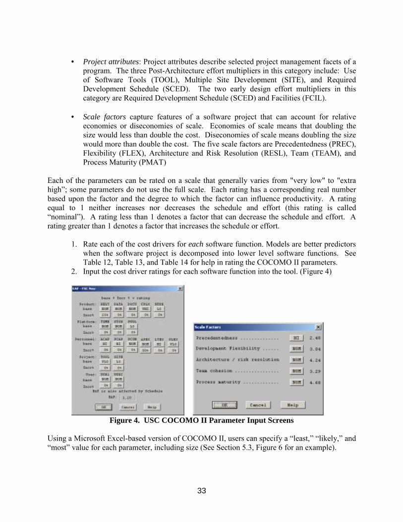
1. Rate each of the cost drivers for each software function. Models are better predictors when the software project is decomposed into lower level software functions. See Table 12, Table 13, and Table 14 for help in rating the COCOMO II parameters.

2. Input the cost driver ratings for each software function into the tool. (Figure 4)

Figure 4. USC COCOMO II Parameter Input Screens

Using a Microsoft Excel-based version of COCOMO II, users can specify a �least,� �likely,� and �most� value for each parameter, including size (See Section 5.3, Figure 6 for an example).

34

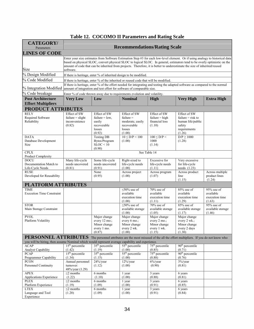
Table 12. COCOMO II Parameters and Rating Scale

CATEGORY/ Parameters Recommendations/Rating Scale

LINES OF CODE

Size

Enter your size estimates from Software Estimation Step #3 for each low-level element. Or if using analogy to historical data based on physical SLOC, convert physical SLOC to logical SLOC. In general, estimators tend to be overly optimistic on the amount of code that can be inherited from projects. Therefore, it is better to underestimate the size of inherited/reused software.

% Design Modified If there is heritage, enter % of inherited design to be modified. % Code Modified If there is heritage, enter % of the inherited or reused code that will be modified.

% Integration Modified If there is heritage, enter % of the effort needed for integrating and testing the adapted software as compared to the normal amount of integration and test effort for software of comparable size.

% Code breakage Enter % of code thrown away due to requirements evolution and volatility. Post Architecture Effort Multipliers

Very Low Low Nominal High Very High Extra High

PRODUCT ATTRIBUTES RELY Required Software Reliability

Effect of SW failure = slight inconvenience (0.82)

Effect of SW failure = low, easily recoverable losses (0.92)

Effect of SW failure = moderate, easily recoverable losses (1.00)

Effect of SW failure = high financial loss (1.10)

Effect of SW failure = risk to human life/public safety requirements (1.26)

DATA Database Development Size

Testing DB Bytes/Program SLOC < 10 (0.90)

10 ≤ D/P < 100 (1.00)

100 ≤ D/P < 1000 (1.14)

D/P ≥ 1000 (1.28)

CPLX Product Complexity

See Table 14

DOCU Documentation Match to Life-Cycle Needs

Many life-cycle needs uncovered (0.81)

Some life-cycle needs uncovered (0.91)

Right-sized to life-cycle needs (1.00)

Excessive for life-cycle needs (1.11)

Very excessive for life-cycle needs (1.23)

RUSE Developed for Reusability

None (0.95)

Across project (1.00)

Across program (1.07)

Across product line (1.15)

Across multiple product lines (1.24)

PLATFORM ATTRIBUTES TIME Execution Time Constraint

≤50% use of available execution time (1.00)

70% use of available execution time (1.11)



STOR Main Storage Constraint

≤50% use of available storage (1.00)

70% use of available storage (1.05)



PVOL Platform Volatility

Major change every 12 mo.; Minor change every 1 mo. (0.87)

Major change every 6 mo.; Minor change every 2 wk. (1.00)

Major change every 2 mo.; Minor change every 1 wk. (1.15)

Major change every 2 wk.; Minor change every 2 days (1.30)

PERSONNEL ATTRIBUTES The personnel attributes are the most misused of the all the effort multipliers. If you do not know who you will be hiring, then assume Nominal which would represent average capability and experience. ACAP Analyst Capability

15th percentile (1.42)





PCAP Programmer Capability






PCON Personnel Continuity

Annual personnel turnover: 48%/year (1.29)

24%/year (1.12)

12%/year (1.00)

6%/year (0.90)

3%/year (0.81)

APEX Applications Experience

≤2 months (1.22)

6 months (1.10)

1 year (1.00)

3 years (0.88)

6 years (0.81)

PLEX Platform Experience

≤2 months (1.19)

6 months (1.09)

1 year (1.00)

3 years (0.91)

6 years (0.85)

LTEX Language and Tool Experience

≤2 months (1.20)

6 months (1.09)

1 year (1.00)

3 years (0.91)

6 years (0.84)

35

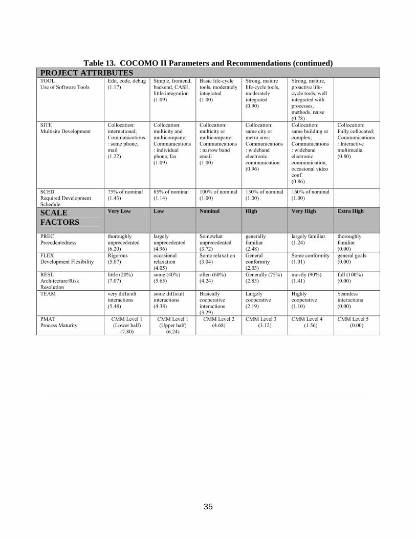
Table 13. COCOMO II Parameters and Recommendations (continued)

PROJECT ATTRIBUTES TOOL Use of Software Tools

Edit, code, debug (1.17)

Simple, frontend, backend, CASE, little integration (1.09)

Basic life-cycle tools, moderately integrated (1.00)

Strong, mature life-cycle tools, moderately integrated (0.90)

Strong, mature, proactive life-cycle tools, well integrated with processes, methods, reuse (0.78)

SITE Multisite Development

Collocation: international; Communications: some phone, mail (1.22)

Collocation: multicity and multicompany; Communications: individual phone, fax (1.09)

Collocation: multicity or multicompany; Communications: narrow band email (1.00)

Collocation: same city or metro area; Communications: wideband electronic communication (0.96)

Collocation: same building or complex; Communications: wideband electronic communication, occasional video conf. (0.86)

Collocation: Fully collocated; Communications: Interactive multimedia (0.80)

SCED Required Development Schedule

75% of nominal (1.43)





SCALE FACTORS

Very Low Low Nominal High Very High Extra High

PREC Precedentedness

thoroughly unprecedented (6.20)

largely unprecedented (4.96)

Somewhat unprecedented (3.72)

generally familiar (2.48)

largely familiar (1.24)

thoroughly familiar (0.00)

FLEX Development Flexibility

Rigorous (5.07)

occasional relaxation (4.05)

Some relaxation (3.04)

General conformity (2.03)

Some conformity (1.01)

general goals (0.00)

RESL Architecture/Risk Resolution

little (20%) (7.07)

some (40%) (5.65)

often (60%) (4.24)

Generally (75%) (2.83)

mostly (90%) (1.41)

full (100%) (0.00)

TEAM very difficult interactions (5.48)

some difficult interactions (4.38)

Basically cooperative interactions (3.29)

Largely cooperative (2.19)

Highly cooperative (1.10)

Seamless interactions (0.00)

PMAT Process Maturity

CMM Level 1 (Lower half)

(7.80)

CMM Level 1 (Upper half)

(6.24)

CMM Level 2 (4.68)

CMM Level 3 (3.12)

CMM Level 4 (1.56)

CMM Level 5 (0.00)

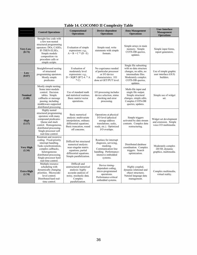
36

Table 14. COCOMO II Complexity Table Control Operations Computational

Operations Device-dependent

Operations Data Management

Operations

User Interface Management Operations

Very Low (0.73)

Straight-line code with a few non-nested

structured programming operators: DOs, CASEs,

IF-THEN-ELSEs. Simple module composition via

procedure calls or simple scripts.

Evaluation of simple expressions: e.g.,

A = B + C * (D �E)

Simple read, write statements with simple

formats.

Simple arrays in main memory. Simple

COTS-DB queries, updates.

Simple input forms, report generators.

Low (0.87)

Straightforward nesting of structured

programming operators. Mostly simple

predicates

Evaluation of moderately level expressions: e.g.,

D = SQRT (B*2-4. * A * C)

No cognizance needed of particular processor

or I/O device characteristics. I/O

done at GET/PUT level.

Single file subsetting with no data structure changes, no edits, no

intermediate files. Moderately complex COTS-DB queries,

updates.

Use of simple graphic user interface (GUI)

builders.

Nominal (1.00)

Mostly simple nesting. Some inter-module control. Decision

tables. Simple callbacks or message

passing, including middleware-supported distributed processing

Use of standard math and statistical routines.

Basic matrix/vector operations.

I/O processing includes device selection, status

checking and error processing.

Multi-file input and single file output. Simple structural

changes, simple edits. Complex COTS-DB

queries, updates.

Simple use of widget set.

High (1.17)

Highly nested structured programming

operators with many compound predicates.

Queue and stack control. Homogeneous, distributed processing. Single processor soft

real-time control.

Basic numerical analysis: multivariate interpolation, ordinary differential equations.

Basic truncation, round off concerns.

Operations at physical I/O level (physical

storage address translations; seeks,

reads, etc.). Optimized I/O overlaps.

Simple triggers activated by data stream contents. Complex data

restructuring.

Widget set development and extension. Simple voice I/O multimedia.

Very High (1.34)

Reentrant and recursive coding. Fixed-priority

interrupt handling. Tasks synchronization,

complex callbacks, heterogeneous

distributed processing. Single-processor hard

real-time control.

Difficult but structured numerical analysis: near-singular matrix

equations, partial differential equations. Simple parallelization.

Routines for interrupt diagnosis, servicing,

masking. Communication line

handling. Performance-intensive embedded

systems.

Distributed database coordination. Complex

triggers. Search optimization.

Moderately complex 2D/3D, dynamic

graphics, multimedia.

Extra High (1.74)

Multiple resource scheduling with

dynamically changing priorities. Microcode-

level control. Distributed hard real-

time control.

Difficult and unstructured numerical

analysis: highly accurate analysis of

noisy, stochastic data. Complex

parallelization.

Device timing-dependent coding, micro-programmed

operations. Performance-critical embedded systems.

Highly coupled, dynamic relational and

object structures. Natural language data

management.

Complex multimedia, virtual reality.

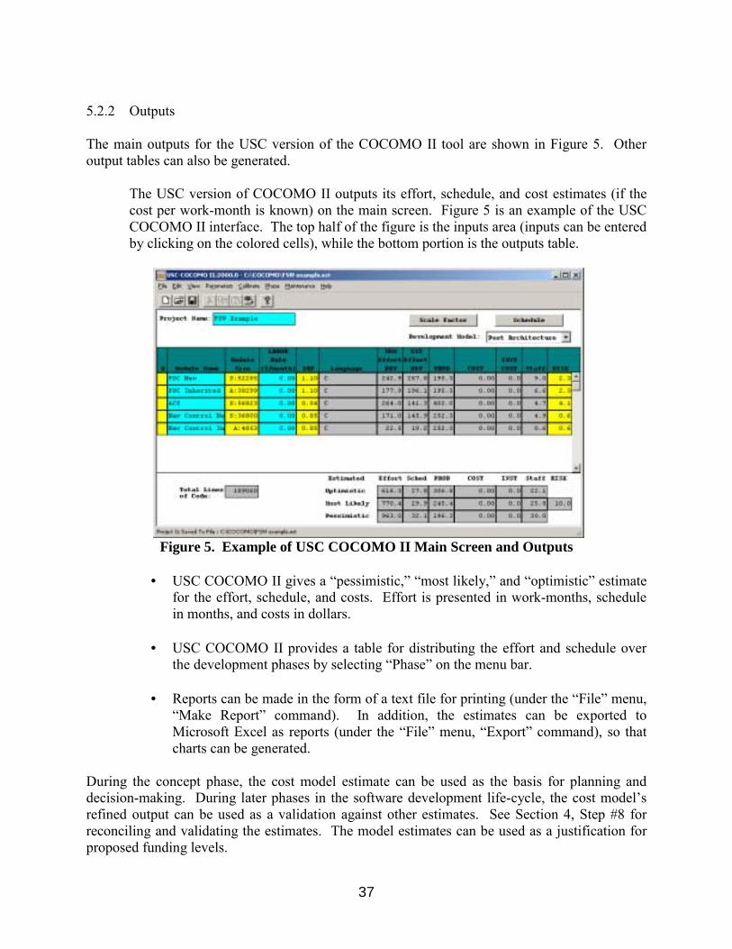
37

5.2.2 Outputs The main outputs for the USC version of the COCOMO II tool are shown in Figure 5. Other output tables can also be generated.

The USC version of COCOMO II outputs its effort, schedule, and cost estimates (if the cost per work-month is known) on the main screen. Figure 5 is an example of the USC COCOMO II interface. The top half of the figure is the inputs area (inputs can be entered by clicking on the colored cells), while the bottom portion is the outputs table.

Figure 5. Example of USC COCOMO II Main Screen and Outputs

• USC COCOMO II gives a �pessimistic,� �most likely,� and �optimistic� estimate

for the effort, schedule, and costs. Effort is presented in work-months, schedule in months, and costs in dollars.

• USC COCOMO II provides a table for distributing the effort and schedule over

the development phases by selecting �Phase� on the menu bar.

• Reports can be made in the form of a text file for printing (under the �File� menu, �Make Report� command). In addition, the estimates can be exported to Microsoft Excel as reports (under the �File� menu, �Export� command), so that charts can be generated.

During the concept phase, the cost model estimate can be used as the basis for planning and decision-making. During later phases in the software development life-cycle, the cost model�s refined output can be used as a validation against other estimates. See Section 4, Step #8 for reconciling and validating the estimates. The model estimates can be used as a justification for proposed funding levels.

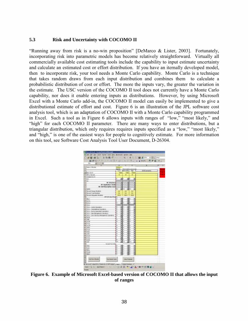
38

5.3 Risk and Uncertainty with COCOMO II �Running away from risk is a no-win proposition� [DeMarco & Lister, 2003]. Fortunately, incorporating risk into parametric models has become relatively straightforward. Virtually all commercially available cost estimating tools include the capability to input estimate uncertainty and calculate an estimated cost or effort distribution. If you have an iternally developed model, then to incorporate risk, your tool needs a Monte Carlo capability. Monte Carlo is a technique that takes random draws from each input distribution and combines them to calculate a probabilistic distribution of cost or effort. The more the inputs vary, the greater the variation in the estimate. The USC version of the COCOMO II tool does not currently have a Monte Carlo capability, nor does it enable entering inputs as distributions. However, by using Microsoft Excel with a Monte Carlo add-in, the COCOMO II model can easily be implemented to give a distributional estimate of effort and cost. Figure 6 is an illustration of the JPL software cost analysis tool, which is an adaptation of COCOMO II with a Monte Carlo capability programmed in Excel. Such a tool as in Figure 6 allows inputs with ranges of �low,� �most likely,� and �high� for each COCOMO II parameter. There are many ways to enter distributions, but a triangular distribution, which only requires requires inputs specified as a �low,� �most likely,� and �high,� is one of the easiest ways for people to cognitively estimate. For more information on this tool, see Software Cost Analysis Tool User Document, D-26304.

Figure 6. Example of Microsoft Excel-based version of COCOMO II that allows the input

of ranges

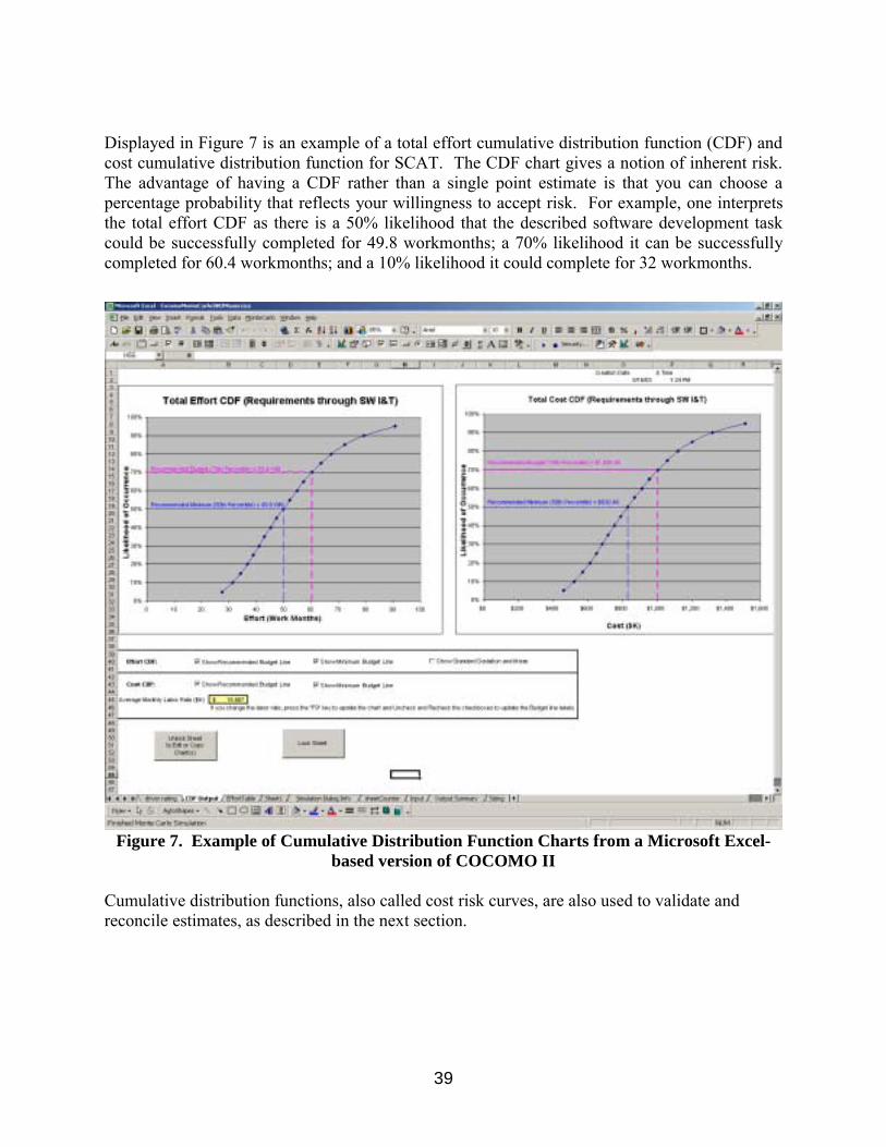
39

Displayed in Figure 7 is an example of a total effort cumulative distribution function (CDF) and cost cumulative distribution function for SCAT. The CDF chart gives a notion of inherent risk. The advantage of having a CDF rather than a single point estimate is that you can choose a percentage probability that reflects your willingness to accept risk. For example, one interprets the total effort CDF as there is a 50% likelihood that the described software development task could be successfully completed for 49.8 workmonths; a 70% likelihood it can be successfully completed for 60.4 workmonths; and a 10% likelihood it could complete for 32 workmonths.

Figure 7. Example of Cumulative Distribution Function Charts from a Microsoft Excel-

based version of COCOMO II Cumulative distribution functions, also called cost risk curves, are also used to validate and reconcile estimates, as described in the next section.

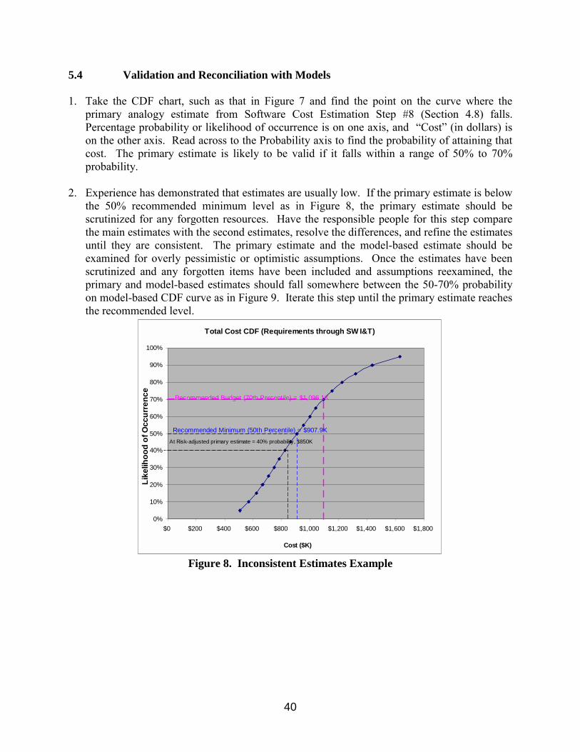
40

5.4 Validation and Reconciliation with Models 1. Take the CDF chart, such as that in Figure 7 and find the point on the curve where the

primary analogy estimate from Software Cost Estimation Step #8 (Section 4.8) falls. Percentage probability or likelihood of occurrence is on one axis, and �Cost� (in dollars) is on the other axis. Read across to the Probability axis to find the probability of attaining that cost. The primary estimate is likely to be valid if it falls within a range of 50% to 70% probability.

2. Experience has demonstrated that estimates are usually low. If the primary estimate is below

the 50% recommended minimum level as in Figure 8, the primary estimate should be scrutinized for any forgotten resources. Have the responsible people for this step compare the main estimates with the second estimates, resolve the differences, and refine the estimates until they are consistent. The primary estimate and the model-based estimate should be examined for overly pessimistic or optimistic assumptions. Once the estimates have been scrutinized and any forgotten items have been included and assumptions reexamined, the primary and model-based estimates should fall somewhere between the 50-70% probability on model-based CDF curve as in Figure 9. Iterate this step until the primary estimate reaches the recommended level.

Total Cost CDF (Requirements through SW I&T)

0%

10%

20%

30%

40%

50%

60%

70%

80%

90%

100%

$0 $200 $400 $600 $800 $1,000 $1,200 $1,400 $1,600 $1,800

Cost ($K)

Like

lihoo

d of

Occ

urre

nce

Recommended Minimum (50th Percentile) = $907.9K

Recommended Budget (70th Percentile) = $1,096.1K

At Risk-adjusted primary estimate = 40% probability, $850K

Figure 8. Inconsistent Estimates Example

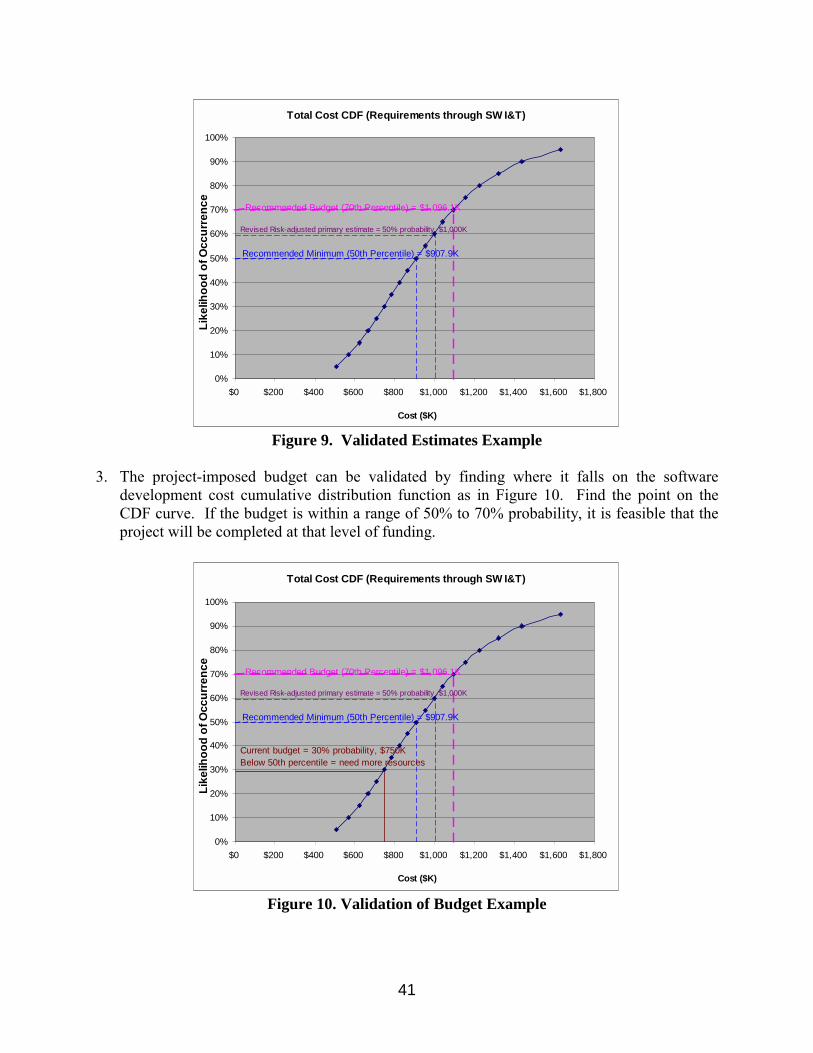
41


0%

10%

20%

30%

40%

50%

60%

70%

80%

90%

100%

$0 $200 $400 $600 $800 $1,000 $1,200 $1,400 $1,600 $1,800

Cost ($K)

Like

lihoo

d of

Occ

urre

nce



Revised Risk-adjusted primary estimate = 50% probability, $1,000K

Figure 9. Validated Estimates Example

3. The project-imposed budget can be validated by finding where it falls on the software

development cost cumulative distribution function as in Figure 10. Find the point on the CDF curve. If the budget is within a range of 50% to 70% probability, it is feasible that the project will be completed at that level of funding.


0%

10%

20%

30%

40%

50%

60%

70%

80%

90%

100%

$0 $200 $400 $600 $800 $1,000 $1,200 $1,400 $1,600 $1,800

Cost ($K)

Like

lihoo

d of

Occ

urre

nce



Revised Risk-adjusted primary estimate = 50% probability, $1,000K

Current budget = 30% probability, $750KBelow 50th percentile = need more resources

Figure 10. Validation of Budget Example

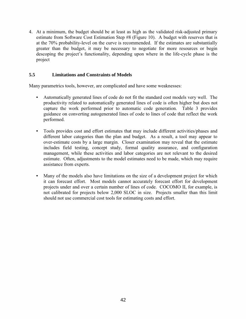
42

4. At a minimum, the budget should be at least as high as the validated risk-adjusted primary estimate from Software Cost Estimation Step #8 (Figure 10). A budget with reserves that is at the 70% probability-level on the curve is recommended. If the estimates are substantially greater than the budget, it may be necessary to negotiate for more resources or begin descoping the project�s functionality, depending upon where in the life-cycle phase is the project

5.5 Limitations and Constraints of Models Many parametrics tools, however, are complicated and have some weaknesses:

• Automatically generated lines of code do not fit the standard cost models very well. The productivity related to automatically generated lines of code is often higher but does not capture the work performed prior to automatic code generation. Table 3 provides guidance on converting autogenerated lines of code to lines of code that reflect the work performed.

• Tools provides cost and effort estimates that may include different activities/phases and

different labor categories than the plan and budget. As a result, a tool may appear to over-estimate costs by a large margin. Closer examination may reveal that the estimate includes field testing, concept study, formal quality assurance, and configuration management, while these activities and labor categories are not relevant to the desired estimate. Often, adjustments to the model estimates need to be made, which may require assistance from experts.

• Many of the models also have limitations on the size of a development project for which

it can forecast effort. Most models cannot accurately forecast effort for development projects under and over a certain number of lines of code. COCOMO II, for example, is not calibrated for projects below 2,000 SLOC in size. Projects smaller than this limit should not use commercial cost tools for estimating costs and effort.

43

6.0 APPENDICES APPENDIX A. ACRONYMS ARR ATLO Readiness Review AT Acceptance Test (DSMS) ATLO Assembly, Test, & Launch Operations BDE Budget Direct Effort CDR Critical Design Review CM Configuration Management COCOMO Constructive Cost Model. Model developed by Dr. Barry Boehm of the USC Center for Software

Engineering COTS Commercial Off-The-Shelf CSE Center for Software Engineering FSW Flight Software FTE Full-Time Equivalent HW Hardware IEEE Institute of Electrical and Electronics Engineers, Inc. I&T Integration and Test IV&V Independent Verification and Validation JPL Jet Propulsion Laboratory NASA National Aeronautics & Space Administration PC Personal Computer PDCR Preliminary Design and Cost Review PDR Preliminary Design Review PERT Program Evaluation and Review Technique PMSR Project Mission System Review QA Quality Assurance ROM Read Only Memory SLOC Source Lines of Code SORCE Software Resource Center SQI Software Quality Improvement SQA Software Quality Assurance SRR Software Requirements Review SW Software TRR Test Readiness Review USC University of Southern California WBS Work Breakdown Structure WM Work - Month

44

APPENDIX B. GLOSSARY Bottom-Up - Pertaining to an activity that starts with the lowest-level components of a hierarchy and proceeds through progressively higher levels; for example, bottom-up design; bottom-up testing. Critical Path – A series of dependent tasks for a project that must be completed as planned to keep the entire project on schedule. Effort - Number of Work-Months a project takes to accomplish a work activity. Source Lines of Code (SLOC) - All source code statements including, Data Declarations, Data Typing statements, Equivalence statements, and Input/Output format statements. SLOC does not include comments, blank lines, data, and non-delivered programmer debug statements. For the purposes of this handbook, SLOC refers to logical lines of code. Logical statements may encompass several physical lines and typically include executable statements, declarations, and compiler directives. A logical statement is a single software instruction, having a defined beginning and ending independent of any relationship to the physical lines on which it is recorded or printed. Software Architecture - The organizational structure of the software or module. [IEEE-STD-610] Software Quality Assurance � Activities performed by the SQA organization to ensure that proper quality assurance processes are selected and used. Software Engineering � Activities performed by the cognizant engineer and developers to unit design, develop code, unit test, and integrate software components. Software Estimates � Software size, effort and cost, schedule and the impact of risks Software Management � Activities performed by the project element manager (PEM), flight software manager, technical lead, and system administration to plan and direct the software project and software configuration management. Software System Engineering � Activities performed by the software architect, software system engineer, and subsystem engineer for functional design, software requirements, and interface specification. Software Test Engineer � Activities performed by a group separate from those involved in software engineering to write test plans and procedures to perform any level of test above unit testing. Does not include test-bed development and support, system-level test support, or ATLO support. Work Breakdown Structure - The WBS subdivides the project into a hierarchical structure of work elements that are each defined, estimated, and tracked. Work – Month � Hours worked in one month ~160 hours.

45

APPENDIX C. DIFFERENCE BETWEEN SOFTWARE COST ESTIMATION STEPS AT DIFFERENT LIFE-CYCLE PHASES If you follow the handbook as it is written, it is most appropriate for projects as they prepare for the Product Design Review and can be easily tailored for other stages of the life-cycle as indicated in Table 15. Mission life-cycle phases and milestones are listed at the top of the table. Software life-cycle phases are arranged in the next row by their relative timing to the mission life-cycle phases. Note that there are differences between the mission life-cycle phases and the software and life-cycle phases. For example, in reality, ATLO, system test, and acceptance do not exactly overlap, but they are displayed that way for simplicity. The software cost estimation steps vary in level of granularity at different phases of the life-cycle. Some steps may be skipped or adapted slightly. In addition, iteration of the steps varies at different life-cycle phases. As a software cost estimate progresses through the life-cycle, the new estimate should be updated to reflect new assumptions.

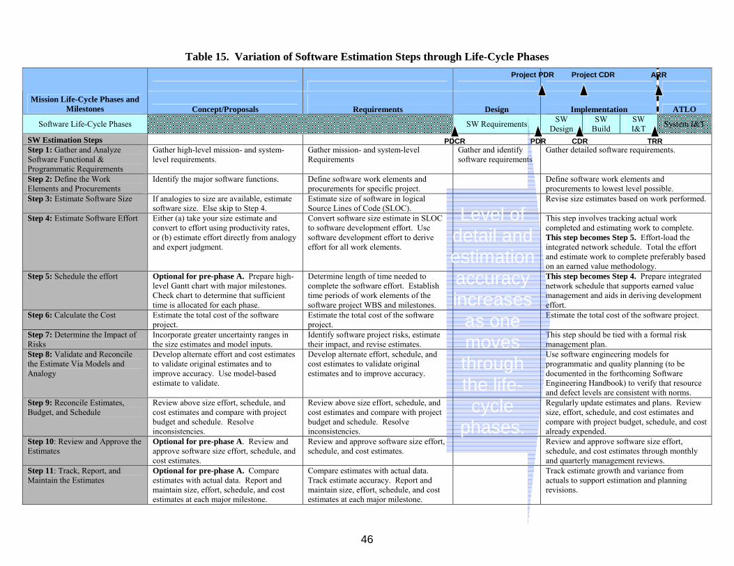
46

Table 15. Variation of Software Estimation Steps through Life-Cycle Phases

Mission Life-Cycle Phases and

Milestones Concept/Proposals

Requirements

Design

Implementation ATLO

Software Life-Cycle Phases SW Requirements SW Design

SW Build

SW I&T System I&T

SW Estimation Steps Step 1: Gather and Analyze Software Functional & Programmatic Requirements

Gather high-level mission- and system-level requirements.

Gather mission- and system-level Requirements

Gather and identify software requirements

Gather detailed software requirements.

Step 2: Define the Work Elements and Procurements

Identify the major software functions. Define software work elements and procurements for specific project.

Define software work elements and procurements to lowest level possible.

Step 3: Estimate Software Size If analogies to size are available, estimate software size. Else skip to Step 4.

Estimate size of software in logical Source Lines of Code (SLOC).

Revise size estimates based on work performed.

Step 4: Estimate Software Effort Either (a) take your size estimate and convert to effort using productivity rates, or (b) estimate effort directly from analogy and expert judgment.

Convert software size estimate in SLOC to software development effort. Use software development effort to derive effort for all work elements.

This step involves tracking actual work completed and estimating work to complete. This step becomes Step 5. Effort-load the integrated network schedule. Total the effort and estimate work to complete preferably based on an earned value methodology.

Step 5: Schedule the effort Optional for pre-phase A. Prepare high-level Gantt chart with major milestones. Check chart to determine that sufficient time is allocated for each phase.

Determine length of time needed to complete the software effort. Establish time periods of work elements of the software project WBS and milestones.

This step becomes Step 4. Prepare integrated network schedule that supports earned value management and aids in deriving development effort.

Step 6: Calculate the Cost Estimate the total cost of the software project.



Step 7: Determine the Impact of Risks

Incorporate greater uncertainty ranges in the size estimates and model inputs.

Identify software project risks, estimate their impact, and revise estimates.

This step should be tied with a formal risk management plan.

Step 8: Validate and Reconcile the Estimate Via Models and Analogy

Develop alternate effort and cost estimates to validate original estimates and to improve accuracy. Use model-based estimate to validate.

Develop alternate effort, schedule, and cost estimates to validate original estimates and to improve accuracy.

Use software engineering models for programmatic and quality planning (to be documented in the forthcoming Software Engineering Handbook) to verify that resource and defect levels are consistent with norms.

Step 9: Reconcile Estimates, Budget, and Schedule

Review above size effort, schedule, and cost estimates and compare with project budget and schedule. Resolve inconsistencies.

Review above size effort, schedule, and cost estimates and compare with project budget and schedule. Resolve inconsistencies.

Regularly update estimates and plans. Review size, effort, schedule, and cost estimates and compare with project budget, schedule, and cost already expended.

Step 10: Review and Approve the Estimates

Optional for pre-phase A. Review and approve software size effort, schedule, and cost estimates.

Review and approve software size effort, schedule, and cost estimates.

Review and approve software size effort, schedule, and cost estimates through monthly and quarterly management reviews.

Step 11: Track, Report, and Maintain the Estimates

Optional for pre-phase A. Compare estimates with actual data. Report and maintain size, effort, schedule, and cost estimates at each major milestone.

Compare estimates with actual data. Track estimate accuracy. Report and maintain size, effort, schedule, and cost estimates at each major milestone.

Track estimate growth and variance from actuals to support estimation and planning revisions.

Project CDRProject PDR ARR

CDR PDR PDCR TRR

Level of detail and estimation accuracy increases

as one moves through the life-cycle

phases.

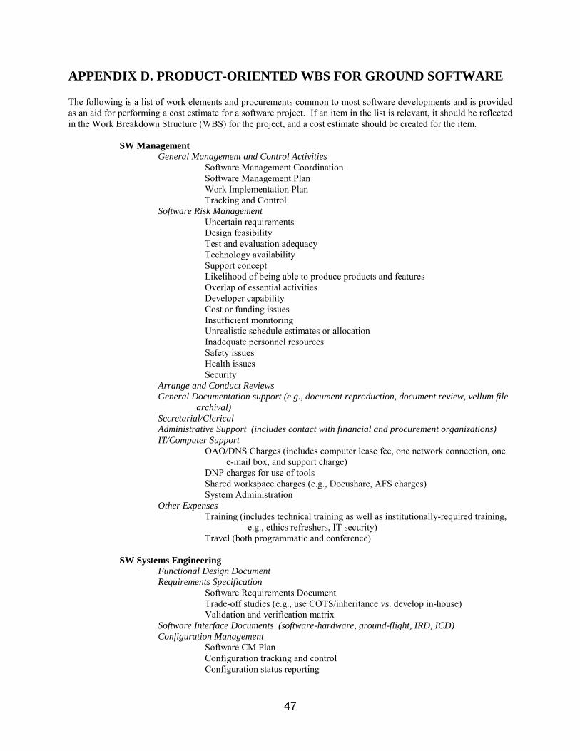
47

APPENDIX D. PRODUCT-ORIENTED WBS FOR GROUND SOFTWARE The following is a list of work elements and procurements common to most software developments and is provided as an aid for performing a cost estimate for a software project. If an item in the list is relevant, it should be reflected in the Work Breakdown Structure (WBS) for the project, and a cost estimate should be created for the item.

SW Management General Management and Control Activities Software Management Coordination Software Management Plan Work Implementation Plan Tracking and Control Software Risk Management

Uncertain requirements Design feasibility Test and evaluation adequacy Technology availability Support concept Likelihood of being able to produce products and features Overlap of essential activities Developer capability Cost or funding issues Insufficient monitoring Unrealistic schedule estimates or allocation Inadequate personnel resources Safety issues Health issues Security

Arrange and Conduct Reviews General Documentation support (e.g., document reproduction, document review, vellum file

archival) Secretarial/Clerical Administrative Support (includes contact with financial and procurement organizations) IT/Computer Support OAO/DNS Charges (includes computer lease fee, one network connection, one

e-mail box, and support charge) DNP charges for use of tools Shared workspace charges (e.g., Docushare, AFS charges) System Administration Other Expenses Training (includes technical training as well as institutionally-required training,

e.g., ethics refreshers, IT security) Travel (both programmatic and conference)

SW Systems Engineering Functional Design Document Requirements Specification Software Requirements Document Trade-off studies (e.g., use COTS/inheritance vs. develop in-house) Validation and verification matrix Software Interface Documents (software-hardware, ground-flight, IRD, ICD) Configuration Management Software CM Plan Configuration tracking and control Configuration status reporting

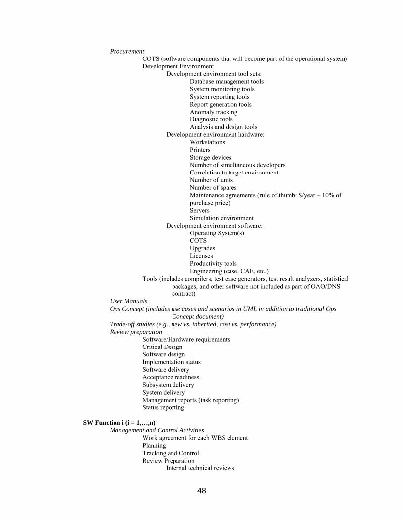
48

Procurement COTS (software components that will become part of the operational system) Development Environment

Development environment tool sets: Database management tools System monitoring tools System reporting tools Report generation tools Anomaly tracking Diagnostic tools Analysis and design tools

Development environment hardware: Workstations Printers Storage devices Number of simultaneous developers Correlation to target environment Number of units Number of spares Maintenance agreements (rule of thumb: $/year � 10% of purchase price) Servers Simulation environment

Development environment software: Operating System(s) COTS Upgrades Licenses Productivity tools

Engineering (case, CAE, etc.) Tools (includes compilers, test case generators, test result analyzers, statistical

packages, and other software not included as part of OAO/DNS contract)

User Manuals Ops Concept (includes use cases and scenarios in UML in addition to traditional Ops

Concept document) Trade-off studies (e.g., new vs. inherited, cost vs. performance) Review preparation

Software/Hardware requirements Critical Design Software design Implementation status Software delivery Acceptance readiness Subsystem delivery System delivery Management reports (task reporting) Status reporting

SW Function i (i = 1,…,n)

Management and Control Activities Work agreement for each WBS element Planning Tracking and Control Review Preparation Internal technical reviews

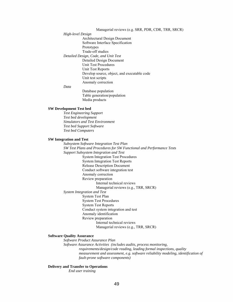
49

Managerial reviews (e.g. SRR, PDR, CDR, TRR, SRCR) High-level Design Architectural Design Document Software Interface Specification Prototypes Trade-off studies Detailed Design, Code, and Unit Test Detailed Design Document Unit Test Procedures Unit Test Reports Develop source, object, and executable code Unit test scripts Anomaly correction Data Database population Table generation/population Media products

SW Development Test bed Test Engineering Support Test bed development Simulators and Test Environment Test bed Support Software

Test bed Computers

SW Integration and Test Subsystem Software Integration Test Plan SW Test Plans and Procedures for SW Functional and Performance Tests Support Subsystem Integration and Test System Integration Test Procedures System Integration Test Reports Release Description Document Conduct software integration test Anomaly correction Review preparation Internal technical reviews Managerial reviews (e.g., TRR, SRCR) System Integration and Test System Test Plan System Test Procedures System Test Reports Conduct system integration and test Anomaly identification Review preparation Internal technical reviews Managerial reviews (e.g., TRR, SRCR)

Software Quality Assurance Software Product Assurance Plan Software Assurance Activities (includes audits, process monitoring,

requirements/design/code reading, leading formal inspections, quality measurement and assessment, e.g. software reliability modeling, identification of fault-prone software components)

Delivery and Transfer to Operations

End user training

50

Computer based training Classroom On-site (includes travel) Video Self-paced

Embedded

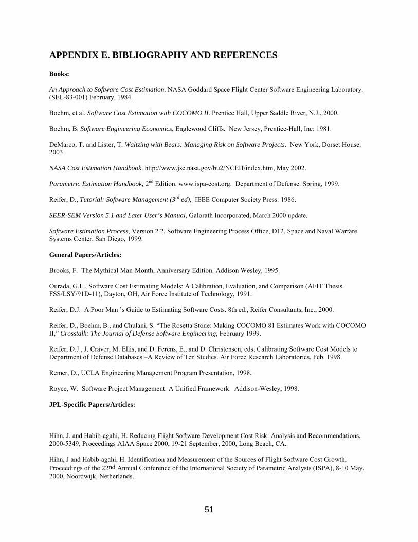
51

APPENDIX E. BIBLIOGRAPHY AND REFERENCES Books: An Approach to Software Cost Estimation. NASA Goddard Space Flight Center Software Engineering Laboratory. (SEL-83-001) February, 1984. Boehm, et al. Software Cost Estimation with COCOMO II. Prentice Hall, Upper Saddle River, N.J., 2000. Boehm, B. Software Engineering Economics, Englewood Cliffs. New Jersey, Prentice-Hall, Inc: 1981. DeMarco, T. and Lister, T. Waltzing with Bears: Managing Risk on Software Projects. New York, Dorset House: 2003. NASA Cost Estimation Handbook. http://www.jsc.nasa.gov/bu2/NCEH/index.htm, May 2002. Parametric Estimation Handbook, 2nd Edition. www.ispa-cost.org. Department of Defense. Spring, 1999. Reifer, D., Tutorial: Software Management (3rd ed), IEEE Computer Society Press: 1986. SEER-SEM Version 5.1 and Later User’s Manual, Galorath Incorporated, March 2000 update. Software Estimation Process, Version 2.2. Software Engineering Process Office, D12, Space and Naval Warfare Systems Center, San Diego, 1999. General Papers/Articles: Brooks, F. The Mythical Man-Month, Anniversary Edition. Addison Wesley, 1995. Ourada, G.L., Software Cost Estimating Models: A Calibration, Evaluation, and Comparison (AFIT Thesis FSS/LSY/91D-11), Dayton, OH, Air Force Institute of Technology, 1991. Reifer, D.J. A Poor Man �s Guide to Estimating Software Costs. 8th ed., Reifer Consultants, Inc., 2000. Reifer, D., Boehm, B., and Chulani, S. �The Rosetta Stone: Making COCOMO 81 Estimates Work with COCOMO II,� Crosstalk: The Journal of Defense Software Engineering, February 1999. Reifer, D.J., J. Craver, M. Ellis, and D. Ferens, E., and D. Christensen, eds. Calibrating Software Cost Models to Department of Defense Databases �A Review of Ten Studies. Air Force Research Laboratories, Feb. 1998. Remer, D., UCLA Engineering Management Program Presentation, 1998. Royce, W. Software Project Management: A Unified Framework. Addison-Wesley, 1998. JPL-Specific Papers/Articles: Hihn, J. and Habib-agahi, H. Reducing Flight Software Development Cost Risk: Analysis and Recommendations, 2000-5349, Proceedings AIAA Space 2000, 19-21 September, 2000, Long Beach, CA. Hihn, J and Habib-agahi, H. Identification and Measurement of the Sources of Flight Software Cost Growth, Proceedings of the 22nd Annual Conference of the International Society of Parametric Analysts (ISPA), 8-10 May, 2000, Noordwijk, Netherlands.

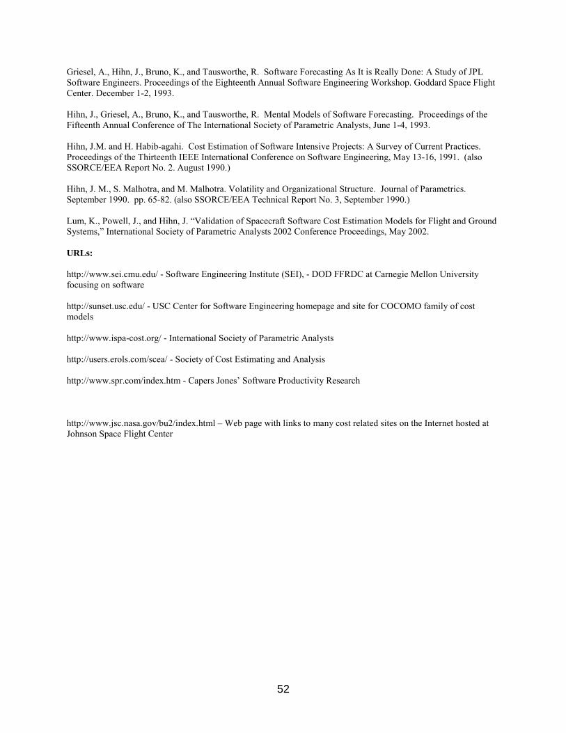
52

Griesel, A., Hihn, J., Bruno, K., and Tausworthe, R. Software Forecasting As It is Really Done: A Study of JPL Software Engineers. Proceedings of the Eighteenth Annual Software Engineering Workshop. Goddard Space Flight Center. December 1-2, 1993. Hihn, J., Griesel, A., Bruno, K., and Tausworthe, R. Mental Models of Software Forecasting. Proceedings of the Fifteenth Annual Conference of The International Society of Parametric Analysts, June 1-4, 1993. Hihn, J.M. and H. Habib-agahi. Cost Estimation of Software Intensive Projects: A Survey of Current Practices. Proceedings of the Thirteenth IEEE International Conference on Software Engineering, May 13-16, 1991. (also SSORCE/EEA Report No. 2. August 1990.) Hihn, J. M., S. Malhotra, and M. Malhotra. Volatility and Organizational Structure. Journal of Parametrics. September 1990. pp. 65-82. (also SSORCE/EEA Technical Report No. 3, September 1990.) Lum, K., Powell, J., and Hihn, J. �Validation of Spacecraft Software Cost Estimation Models for Flight and Ground Systems,� International Society of Parametric Analysts 2002 Conference Proceedings, May 2002. URLs: http://www.sei.cmu.edu/ - Software Engineering Institute (SEI), - DOD FFRDC at Carnegie Mellon University focusing on software http://sunset.usc.edu/ - USC Center for Software Engineering homepage and site for COCOMO family of cost models http://www.ispa-cost.org/ - International Society of Parametric Analysts http://users.erols.com/scea/ - Society of Cost Estimating and Analysis http://www.spr.com/index.htm - Capers Jones� Software Productivity Research http://www.jsc.nasa.gov/bu2/index.html � Web page with links to many cost related sites on the Internet hosted at Johnson Space Flight Center

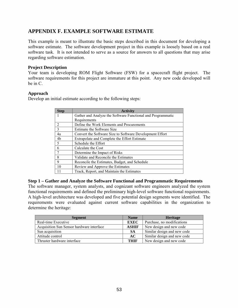
53

APPENDIX F. EXAMPLE SOFTWARE ESTIMATE This example is meant to illustrate the basic steps described in this document for developing a software estimate. The software development project in this example is loosely based on a real software task. It is not intended to serve as a source for answers to all questions that may arise regarding software estimation. Project Description Your team is developing ROM Flight Software (FSW) for a spacecraft flight project. The software requirements for this project are immature at this point. Any new code developed will be in C. Approach Develop an initial estimate according to the following steps:

Step 1 – Gather and Analyze the Software Functional and Programmatic Requirements The software manager, system analysts, and cognizant software engineers analyzed the system functional requirements and defined the preliminary high-level software functional requirements. A high-level architecture was developed and five potential design segments were identified. The requirements were evaluated against current software capabilities in the organization to determine the heritage:

Segment Name Heritage Real-time Executive EXEC Purchase, no modifications Acquisition Sun Sensor hardware interface ASHIF New design and new code Sun acquisition SA Similar design and new code Attitude control AC Similar design and new code Thruster hardware interface THIF New design and new code

Step Activity 1 Gather and Analyze the Software Functional and Programmatic

Requirements 2 Define the Work Elements and Procurements 3 Estimate the Software Size 4a Convert the Software Size to Software Development Effort 4b Extrapolate and Complete the Effort Estimate 5 Schedule the Effort 6 Calculate the Cost 7 Determine the Impact of Risks 8 Validate and Reconcile the Estimates 9 Reconcile the Estimates, Budget, and Schedule 10 Review and Approve the Estimates 11 Track, Report, and Maintain the Estimates

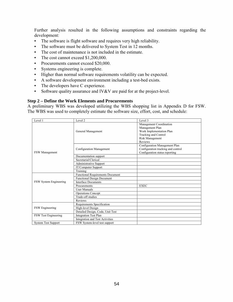
54

Further analysis resulted in the following assumptions and constraints regarding the development: • The software is flight software and requires very high reliability. • The software must be delivered to System Test in 12 months. • The cost of maintenance is not included in the estimate. • The cost cannot exceed $1,200,000. • Procurements cannot exceed $20,000. • Systems engineering is complete. • Higher than normal software requirements volatility can be expected. • A software development environment including a test-bed exists. • The developers have C experience. • Software quality assurance and IV&V are paid for at the project-level.

Step 2 – Define the Work Elements and Procurements A preliminary WBS was developed utilizing the WBS shopping list in Appendix D for FSW. The WBS was used to completely estimate the software size, effort, cost, and schedule:

Level 1 Level 2 Level 3 General Management

Management Coordination Management Plan Work Implementation Plan Tracking and Control Risk Management Reviews

Configuration Management

Configuration Management Plan Configuration tracking and control Configuration status reporting

Documentation support Secretarial/Clerical Administrative Support IT/Computer Support

FSW Management

Training Functional Requirements Document Functional Design Document Interface Documents Procurements EXEC User Manuals Operations Concept Trade-off studies

FSW System Engineering

Reviews Requirements Specification High-level Design

FSW Engineering

Detailed Design, Code, Unit Test Integration Test Plan FSW Test Engineering Integration and Test Activities

System Test Support FSW System-level test support

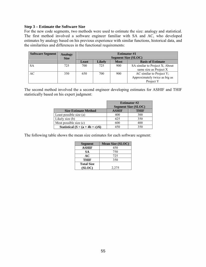
55

Step 3 – Estimate the Software Size For the new code segments, two methods were used to estimate the size: analogy and statistical. The first method involved a software engineer familiar with SA and AC, who developed estimates by analogy based on his previous experience with similar functions, historical data, and the similarities and differences in the functional requirements:

Software Segment Estimator #1 Segment Size (SLOC)

Analogy Size

Least Likely Most Basis of Estimate SA 725 700 725 900 SA similar to Project X; About

same size as Project X AC 350 650 700 900 AC similar to Project Y;

Approximately twice as big as Project Y

The second method involved the a second engineer developing estimates for ASHIF and THIF statistically based on his expert judgment:

Estimator #2 Segment Size (SLOC)

Size Estimate Method ASHIF THIF Least possible size (a) 400 300 Likely size (b) 425 350 Most possible size (c) 600 400

Statistical (S = (a + 4b + c)/6) 450 350 The following table shows the mean size estimates for each software segment:

Segment Mean Size (SLOC) ASHIF 450

SA 750 AC 725

THIF 350 Total Size (SLOC) 2,275

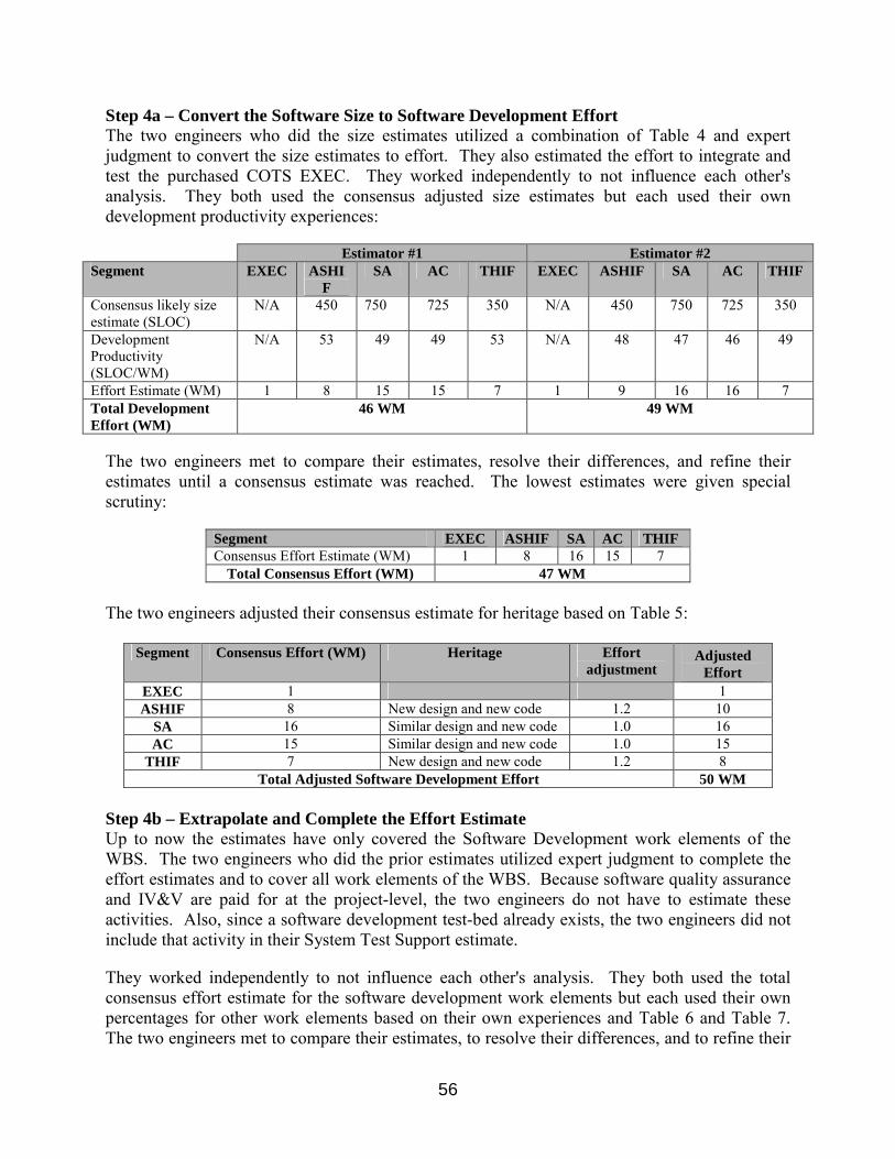
56

Step 4a – Convert the Software Size to Software Development Effort The two engineers who did the size estimates utilized a combination of Table 4 and expert judgment to convert the size estimates to effort. They also estimated the effort to integrate and test the purchased COTS EXEC. They worked independently to not influence each other's analysis. They both used the consensus adjusted size estimates but each used their own development productivity experiences:

Estimator #1 Estimator #2 Segment EXEC ASHI

F SA AC THIF EXEC ASHIF SA AC THIF

Consensus likely size estimate (SLOC)

N/A 450 750 725 350 N/A 450 750 725 350

Development Productivity (SLOC/WM)

N/A 53 49 49 53 N/A 48 47 46 49

Effort Estimate (WM) 1 8 15 15 7 1 9 16 16 7 Total Development Effort (WM)

46 WM 49 WM

The two engineers met to compare their estimates, resolve their differences, and refine their estimates until a consensus estimate was reached. The lowest estimates were given special scrutiny:

Segment EXEC ASHIF SA AC THIF Consensus Effort Estimate (WM) 1 8 16 15 7

Total Consensus Effort (WM) 47 WM The two engineers adjusted their consensus estimate for heritage based on Table 5:

Segment Consensus Effort (WM) Heritage Effort adjustment

Adjusted Effort

EXEC 1 1 ASHIF 8 New design and new code 1.2 10

SA 16 Similar design and new code 1.0 16 AC 15 Similar design and new code 1.0 15

THIF 7 New design and new code 1.2 8 Total Adjusted Software Development Effort 50 WM

Step 4b – Extrapolate and Complete the Effort Estimate Up to now the estimates have only covered the Software Development work elements of the WBS. The two engineers who did the prior estimates utilized expert judgment to complete the effort estimates and to cover all work elements of the WBS. Because software quality assurance and IV&V are paid for at the project-level, the two engineers do not have to estimate these activities. Also, since a software development test-bed already exists, the two engineers did not include that activity in their System Test Support estimate.

They worked independently to not influence each other's analysis. They both used the total consensus effort estimate for the software development work elements but each used their own percentages for other work elements based on their own experiences and Table 6 and Table 7. The two engineers met to compare their estimates, to resolve their differences, and to refine their

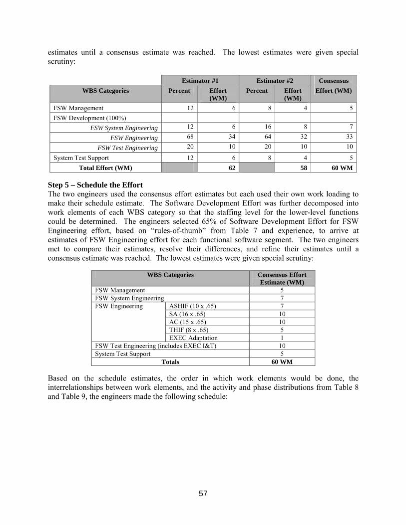
57

estimates until a consensus estimate was reached. The lowest estimates were given special scrutiny:

Estimator #1 Estimator #2 Consensus WBS Categories Percent Effort

(WM) Percent Effort

(WM) Effort (WM)

FSW Management 12 6 8 4 5 FSW Development (100%)

FSW System Engineering 12 6 16 8 7

FSW Engineering 68 34 64 32 33

FSW Test Engineering 20 10 20 10 10

System Test Support 12 6 8 4 5 Total Effort (WM) 62 58 60 WM

Step 5 – Schedule the Effort The two engineers used the consensus effort estimates but each used their own work loading to make their schedule estimate. The Software Development Effort was further decomposed into work elements of each WBS category so that the staffing level for the lower-level functions could be determined. The engineers selected 65% of Software Development Effort for FSW Engineering effort, based on �rules-of-thumb� from Table 7 and experience, to arrive at estimates of FSW Engineering effort for each functional software segment. The two engineers met to compare their estimates, resolve their differences, and refine their estimates until a consensus estimate was reached. The lowest estimates were given special scrutiny:

WBS Categories Consensus Effort Estimate (WM)

FSW Management 5 FSW System Engineering 7

ASHIF (10 x .65) 7 SA (16 x .65) 10 AC (15 x .65) 10 THIF (8 x .65) 5

FSW Engineering

EXEC Adaptation 1 FSW Test Engineering (includes EXEC I&T) 10 System Test Support 5

Totals 60 WM Based on the schedule estimates, the order in which work elements would be done, the interrelationships between work elements, and the activity and phase distributions from Table 8 and Table 9, the engineers made the following schedule:

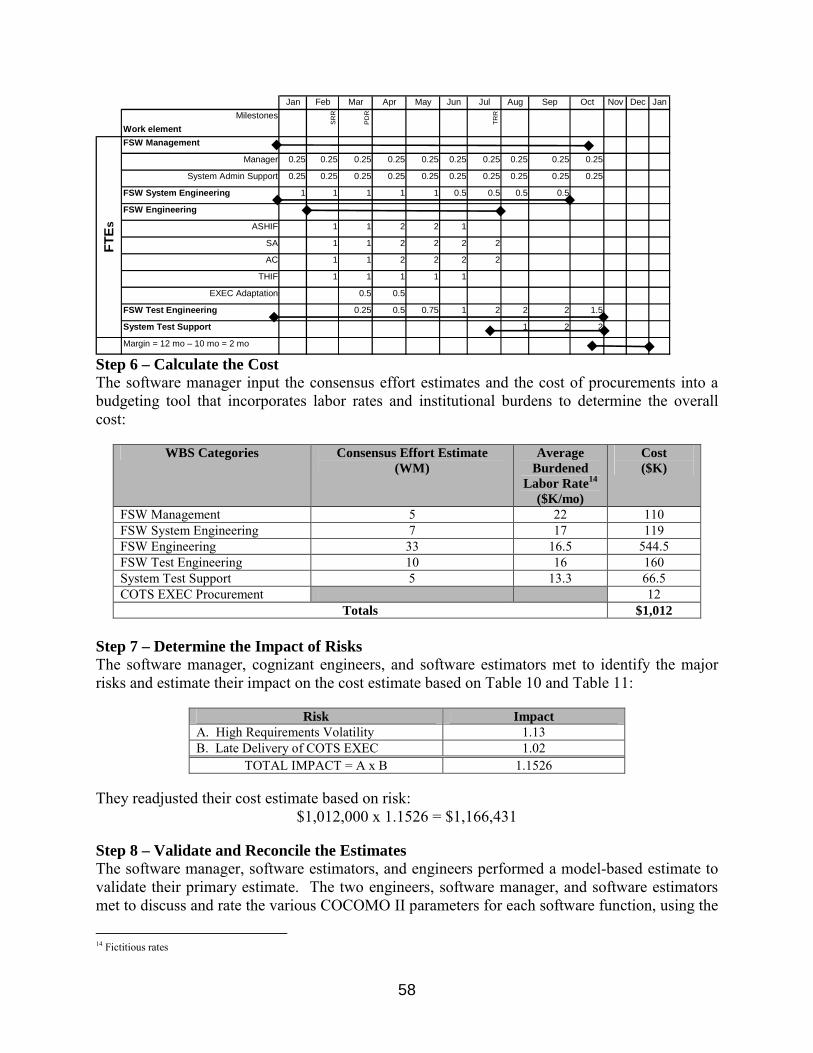
58

Jan Feb Mar Apr May Jun Jul Aug Sep Oct Nov Dec JanMilestones

Work elementFSW Management

Manager 0.25 0.25 0.25 0.25 0.25 0.25 0.25 0.25 0.25 0.25

System Admin Support 0.25 0.25 0.25 0.25 0.25 0.25 0.25 0.25 0.25 0.25

FSW System Engineering 1 1 1 1 1 0.5 0.5 0.5 0.5

FSW Engineering

ASHIF 1 1 2 2 1

SA 1 1 2 2 2 2

AC 1 1 2 2 2 2

THIF 1 1 1 1 1

EXEC Adaptation 0.5 0.5

FSW Test Engineering 0.25 0.5 0.75 1 2 2 2 1.5

System Test Support 1 2 2

Margin = 12 mo – 10 mo = 2 mo

TRR

SRR

PDR

FTEs

Step 6 – Calculate the Cost The software manager input the consensus effort estimates and the cost of procurements into a budgeting tool that incorporates labor rates and institutional burdens to determine the overall cost:

WBS Categories Consensus Effort Estimate (WM)

Average Burdened

Labor Rate14 ($K/mo)

Cost ($K)

FSW Management 5 22 110 FSW System Engineering 7 17 119 FSW Engineering 33 16.5 544.5 FSW Test Engineering 10 16 160 System Test Support 5 13.3 66.5 COTS EXEC Procurement 12

Totals $1,012 Step 7 – Determine the Impact of Risks The software manager, cognizant engineers, and software estimators met to identify the major risks and estimate their impact on the cost estimate based on Table 10 and Table 11:

Risk Impact A. High Requirements Volatility 1.13 B. Late Delivery of COTS EXEC 1.02

TOTAL IMPACT = A x B 1.1526 They readjusted their cost estimate based on risk:

$1,012,000 x 1.1526 = $1,166,431 Step 8 – Validate and Reconcile the Estimates The software manager, software estimators, and engineers performed a model-based estimate to validate their primary estimate. The two engineers, software manager, and software estimators met to discuss and rate the various COCOMO II parameters for each software function, using the

14 Fictitious rates

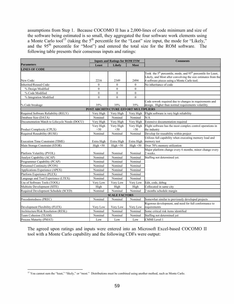
59

assumptions from Step 1. Because COCOMO II has a 2,000-lines of code minimum and size of the software being estimated is so small, they aggregated the four software work elements using a Monte Carlo tool15 (taking the 5th percentile for the �Least� size input, the mode for �Likely,� and the 95th percentile for �Most�) and entered the total size for the ROM software. The following table presents their consensus inputs and ratings:

Inputs and Ratings for ROM FSW Parameters Least Likely Most

Comments

LINES OF CODE

New Code: 2216 2349 2494

Took the 5th percentile, mode, and 95th percentile for Least, Likely, and Most after convolving the size estimates from the 4 software pieces using a Monte Carlo tool.

Inherited/Reused Code: 0 0 0 No inheritance of code % Design Modified 0 0 0 % Code Modified 0 0 0 % Integration Modified 0 0 0

% Code breakage 35% 35% 35% Code rework required due to changes in requirements and design. Higher than normal requirements volatility.

POST ARCHITECTURE EFFORT MULTIPLIERS Required Software Reliability (RELY) Very High Very High Very High Flight software is very high reliability Database Size (DATA) Nominal Nominal Nominal N/A Documentation Match to Lifecycle Needs (DOCU) Very High Very High Very High Extensive documentation required

Product Complexity (CPLX) Very High

+50 Very High

+50 Very High

+50 Flight software has the most complex control operations in the industry

Required Reusability (RUSE) Nominal Nominal Nominal Develop for reusability within project

Execution Time Constraint (TIME) Extra High Extra High Extra High Utilizes full capability when executing memory load and memory test

Main Storage Constraint (STOR) High +50 High +50 High +50 Over 70% memory utilization

Platform Volatility (PVOL) Nominal Nominal Nominal Major platform change every 6 months, minor change every 2 weeks.

Analyst Capability (ACAP) Nominal Nominal Nominal Programmer Capability (PCAP) Nominal Nominal Nominal Personnel Continuity (PCON) Nominal Nominal Nominal Applications Experience (APEX) Nominal Nominal Nominal Platform Experience (PLEX) Nominal Nominal Nominal Language and Tool Experience (LTEX) Nominal Nominal Nominal

Staffing not determined yet.

Use of Software Tools (TOOL) Very Low Very Low Very Low Edit, code, debug Multisite Development (SITE) High High High Collocated in same city Required Development Schedule (SCED) Nominal Nominal Nominal 2 months schedule margin

SCALE FACTORS Precedentedness (PREC) Nominal Nominal Nominal Somewhat similar to previously developed projects

Development Flexibility (FLEX) Very Low Very Low Very Low Rigorous development, and need for full conformance to requirements

Architecture/Risk Resolution (RESL) Nominal Nominal Nominal Some critical risk items identified Team Cohesion (TEAM) Nominal Nominal Nominal Staffing not determined yet Process Maturity (PMAT) Low Low Low CMMI Level 1

The agreed upon ratings and inputs were entered into an Microsoft Excel-based COCOMO II tool with a Monte Carlo capability and the following CDFs were output:

15 You cannot sum the �least,� �likely,� or �most.� Distributions must be combined using another method, such as Monte Carlo.

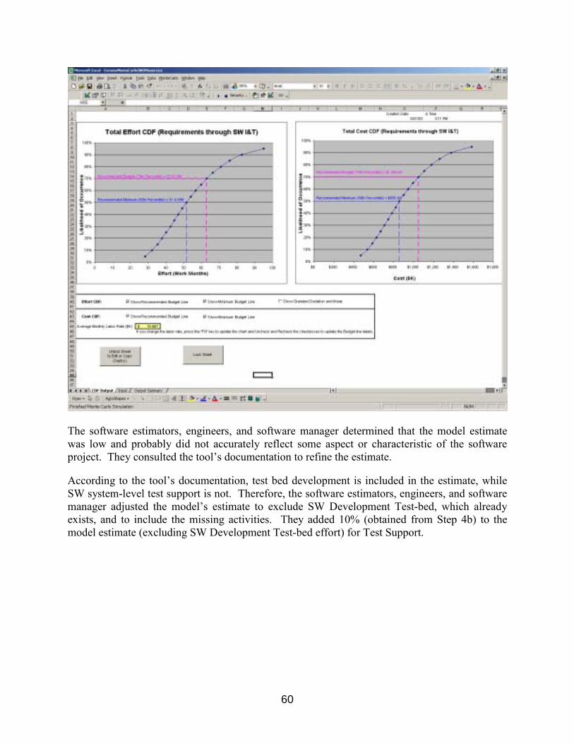
60

The software estimators, engineers, and software manager determined that the model estimate was low and probably did not accurately reflect some aspect or characteristic of the software project. They consulted the tool�s documentation to refine the estimate. According to the tool�s documentation, test bed development is included in the estimate, while SW system-level test support is not. Therefore, the software estimators, engineers, and software manager adjusted the model�s estimate to exclude SW Development Test-bed, which already exists, and to include the missing activities. They added 10% (obtained from Step 4b) to the model estimate (excluding SW Development Test-bed effort) for Test Support.

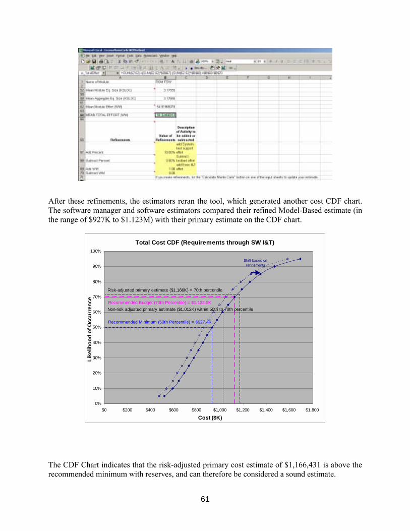
61

After these refinements, the estimators reran the tool, which generated another cost CDF chart. The software manager and software estimators compared their refined Model-Based estimate (in the range of $927K to $1.123M) with their primary estimate on the CDF chart.


0%

10%

20%

30%

40%

50%

60%

70%

80%

90%

100%

$0 $200 $400 $600 $800 $1,000 $1,200 $1,400 $1,600 $1,800

Cost ($K)

Like

lihoo

d of

Occ

urre

nce



Shift based on refinements

Risk-adjusted primary estimate ($1,166K) > 70th percentile

Non-risk adjusted primary estimate ($1,012K) within 50th to 70th percentile

The CDF Chart indicates that the risk-adjusted primary cost estimate of $1,166,431 is above the recommended minimum with reserves, and can therefore be considered a sound estimate.

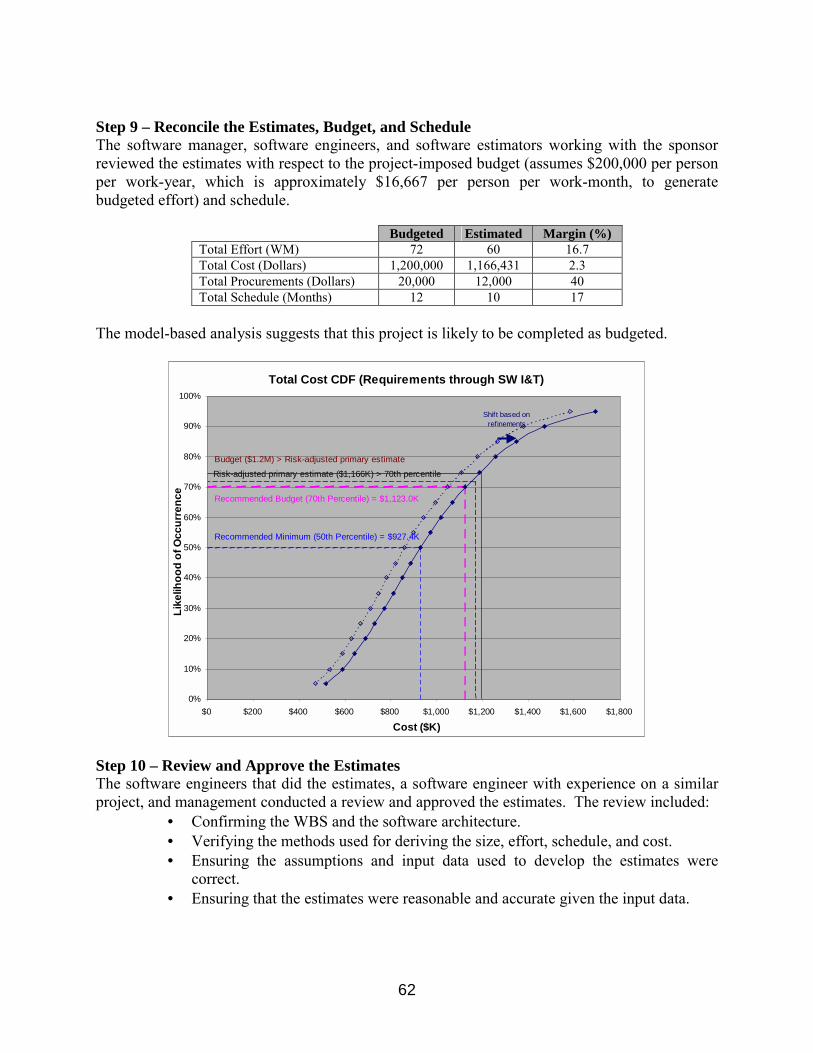
62

Step 9 – Reconcile the Estimates, Budget, and Schedule The software manager, software engineers, and software estimators working with the sponsor reviewed the estimates with respect to the project-imposed budget (assumes $200,000 per person per work-year, which is approximately $16,667 per person per work-month, to generate budgeted effort) and schedule.

Budgeted Estimated Margin (%) Total Effort (WM) 72 60 16.7 Total Cost (Dollars) 1,200,000 1,166,431 2.3 Total Procurements (Dollars) 20,000 12,000 40 Total Schedule (Months) 12 10 17

The model-based analysis suggests that this project is likely to be completed as budgeted.


0%

10%

20%

30%

40%

50%

60%

70%

80%

90%

100%

$0 $200 $400 $600 $800 $1,000 $1,200 $1,400 $1,600 $1,800

Cost ($K)

Like

lihoo

d of

Occ

urre

nce



Shift based on refinements

Risk-adjusted primary estimate ($1,166K) > 70th percentileBudget ($1.2M) > Risk-adjusted primary estimate

Step 10 – Review and Approve the Estimates The software engineers that did the estimates, a software engineer with experience on a similar project, and management conducted a review and approved the estimates. The review included:

• Confirming the WBS and the software architecture. • Verifying the methods used for deriving the size, effort, schedule, and cost. • Ensuring the assumptions and input data used to develop the estimates were

correct. • Ensuring that the estimates were reasonable and accurate given the input data.

63

Step 11 – Track, Report, and Maintain the Estimates The estimate was then archived in a historical database. The following information was recorded with the official software estimates for the project:

• Project contextual and supporting information − Project name − Software organization − Platform − Language − Estimation method(s) and assumptions − Date(s) of approved estimate(s) • Estimated and actual size, effort, cost, and cost of procurements by WBS

work element • Planned and actual schedule dates of major milestones and reviews • Identified risks and their estimated and actual impacts

These estimates were compared with other archived estimates in the database to check the accuracy of the software estimates over time. The estimates were tracked to identify when and by how much the project was over-running or under-running the estimates. Any discrepancies between the current and past estimates and budgets were then resolved.