Hamiltonian long-wave expansions for water waves over a

Proc. R. Soc. A (2005) 461, 839–873doi:10.1098/rspa.2004.1367

Published online 25 January 2005

Hamiltonian long-wave expansions forwater waves over a rough bottom

By Walter Craig1, Philippe Guyenne

1,

David P. Nicholls2

and Catherine Sulem3

1Department of Mathematics & Statistics,McMaster University, 1280 Main Street West, Hamilton,Ontario L8S 4K1, Canada ([email protected])

2Department of Mathematics, University of Notre Dame,Notre Dame, IN 46556-4618, USA

3Department of Mathematics, University of Toronto,Toronto, Ontario M5S 3G3, Canada

This paper is a study of the problem of nonlinear wave motion of the free surfaceof a body of fluid with a periodically varying bottom. The object is to describethe character of wave propagation in a long-wave asymptotic regime, extending theresults of R. Rosales & G. Papanicolaou (1983 Stud. Appl. Math. 68, 89–102) onperiodic bottoms for two-dimensional flows. We take the point of view of perturbationof a Hamiltonian system dependent on a small scaling parameter, with the startingpoint being Zakharov’s Hamiltonian (V. E. Zakharov 1968 J. Appl. Mech. Tech.Phys. 9, 1990–1994) for the Euler equations for water waves. We consider bottomtopography which is periodic in horizontal variables on a short length-scale, with theamplitude of variation being of the same order as the fluid depth. The bottom mayalso exhibit slow variations at the same length-scale as, or longer than, the orderof the wavelength of the surface waves. We do not take up the question of randombottom variations, a topic which is considered in Rosales & Papanicolaou (1983).

In the two-dimensional case of waves in a channel, we give an alternate derivation ofthe effective Korteweg–de Vries (KdV) equation that is obtained in Rosales & Papan-icolaou (1983). In addition, we obtain effective Boussinesq equations that describethe motion of bidirectional long waves, in cases in which the bottom possesses bothshort and long-scale variations. In certain cases we also obtain unidirectional equa-tions that are similar to the KdV equation. In three dimensions we obtain effectivethree-dimensional long-wave equations in a Boussinesq scaling regime, and again incertain cases an effective Kadomtsev–Petviashvili (KP) system in the appropriateunidirectional limit.

The computations for these results are performed in the framework of an asymp-totic analysis of multiple-scale operators. In the present case this involves theDirichlet–Neumann operator for the fluid domain which takes into account the vari-ations in bottom topography as well as the deformations of the free surface fromequilibrium.

Keywords: water waves; variable depth; long-wave asymptotics;Hamiltonian perturbation theory

Received 4 December 2003Accepted 14 June 2004 839

c© 2005 The Royal Society

840 W. Craig and others

1. Introduction

Because of its relevance to coastal engineering, surface water wave propagation inthe presence of an uneven bottom has been studied for many years. The charac-ter of coastal wave dynamics can be very complex; waves are strongly affected bythe bottom through shoaling and the resulting variations in local linear wave speed,with the subsequent effects of refraction, diffraction and reflection. Nonlinear effects,which influence waves of appreciable steepness even in the simplest of cases, haveadditional components due to wave–bottom as well as nonlinear wave–wave interac-tions, as is seen, for example, in depth-induced breaking. The presence of bottomtopography in the fluid domain introduces additional space- and time-scales to theclassical perturbation problem. The resulting nonlinear waves can have a great influ-ence on sediment transport and the formation of shoals and sandbars in near-shoreregions: effects which are strongly felt over the longest time-scales of the problem.It is therefore of central importance to understand the basic equations with whichthey are described.

This paper is a reassessment and extension of the work of Rosales & Papanicolaou(1983) on the long-wave limit of the free-surface problem of water waves in thepresence of a fluid domain of variable depth. It has been a general principle inthe study of free-surface water waves that the long-wave asymptotic scaling regimedescribes many of the principal aspects of the dynamics of wave motion. This is thefocus of the present work, in which we study the effect of a periodic variation ofthe bottom on the long-wavelength limit of free-surface water waves. Analysing theBoussinesq scaling regime, we derive effective, or homogenized coefficients for theresulting system of nonlinear dispersive equations, which is related to the classicalBoussinesq system. When considering initial data which are specifically arranged toemphasize wave motion in one direction, we derive the effective coefficients for theresulting Korteweg–de Vries (KdV) equation. Our analysis poses no assumptions onthe amplitude nor the slope of the bottom variations; they may be considered ofO(1). The analysis carries through to the three-dimensional case, where we derive atwo-dimensional Boussinesq-like system and expressions for its effective coefficientsin the first case, and a Kadomtsev–Petviashvili (KP) system in the case of wavemotion in one direction alone. Because of the explicit nature of our description ofthe long-wave perturbation analysis, and the resulting expressions for the effectivecoefficients of the long-wave equations, we can make several general observations.First is the fact that, among bottom variations with fixed mean depth, the linearwave speed of long waves is slower than that of constant depth, strictly so for non-zero perturbations. This has previously been noted in Rosales & Papanicolaou (1983)in the two-dimensional problem. Secondly, we give numerical computations of theeffective coefficients of nonlinearity and of dispersion in typical cases. Our conclusionis that, for large bottom variations, nonlinear effects dominate dispersive ones whenthe amplitude of bottom variations tends to the shoaling limit (with the mean depthfixed). However, the balance of dispersion to nonlinearity is maintained through aremarkably large range, a fact which tends to further justify the use of the Boussinesqand KdV approximations in the homogenization limit.

We extend the results of Rosales & Papanicolaou (1983) on periodic bottom bound-aries to cases in which the bottom varies over long spatial scales, in addition to theperiodic variations on a length-scale of O(1). This is a class of problems of flows

Proc. R. Soc. A (2005)

Long-wave expansions over a rough bottom 841

over obstacles which has been of interest for many years, and which has most oftenbeen treated without the presence of the short-scale periodic bottom variations. Theliterature is very extensive, and we cite in particular the papers of Johnson (1973),Whitham (1974), Miles (1979), Newell (1985), Nachbin & Papanicolaou (1992), Mei& Liu (1993), van Groesen & Pudjaprasetya (1993), Yoon & Liu (1994) and Kirby(1997). In our analysis, in the case in which the bottom topography varies on thesame length scale as the long waves of our scaling regime, we find a well-definedBoussinesq system with effective coefficients which are functions of the slow spatialvariables X = εx. The three-dimensional Boussinesq regime is similar, as is its rel-evance to flows over three-dimensional obstacles. The resulting Hamiltonian partialdifferential equations (PDEs), which are nonlinear dispersive equations with vari-able coefficients, are interesting in their own right. The derivation of an effectiveKdV equation is a more subtle matter, and may be a little artificial as significantbottom topography gives rise to scattering effects which for solutions of the waterwaves problem will violate any ansatz of unidirectionality. Nonetheless, there areseveral special situations in which one-way equations would make sense, in partic-ular where the slow variations of the bottom topography are small, where the slowvariations are of very gradual slope, or a combination of the two. We analyse thesesituations, giving a criterion under which a KdV scaling regime exists, and derivingthe new form of the KdV equation when it does. In the most compelling cases, theeffective equation governing unidirectional wave motion is the KdV equation withvariable coefficients of nonlinearity and dispersion, with an additional equation for awave component which propagates in the opposite direction, due to scattering fromthe variable bottom topography. The scattered wave is generated after the passageof the initial wave form; it is described by a scalar wave equation with forcing termsformed from the solution of the variable coefficient KdV equation. In many ways thisparallels the work of van Groesen & Pudjaprasetya (1993), although we augment ourderivation with an estimate of the time of validity of the approximation in the variousregimes of interest. There are a few differences in the conclusions as well. Our resultsextend to unidirectional cases in three dimensions, with the same proviso, giving risewhere appropriate to KP-like systems of PDEs.

Our analysis is based on the point of view of the water waves problem as a Hamil-tonian system, and we treat the perturbation problem given by the long-wavelengthscaling limit as a problem in systematic Hamiltonian perturbation theory. The start-ing point is the water waves Hamiltonian originally due to Zakharov (1968), as repre-sented by Craig & Sulem (1993) using the Dirichlet–Neumann operator to express theDirichlet integral for the velocity potential over the fluid domain. The expansion ofthe Hamiltonian in a small parameter which governs the long-wave/small amplitudeasymptotic regime follows a method given in Craig & Groves (1994) and Craig et al.(2004). We employ an expression for the Dirichlet–Neumann operator in the case ofa variable bottom which is similar to those of Liu & Yue (1998) and Smith (1998).Using a theory of multiple-scale expansions for Fourier multiplier operators given inCraig et al. (1992), and results on scale separation, we identify explicit expressionsfor the effective coefficients of the limiting long-wave problems. The fast Fouriertransform is used in the numerical evaluation of these coefficients. In an appendixwe give a concise derivation of the full Taylor expansion of the Dirichlet–Neumannoperator in the present case, with perturbed free-surface and non-constant bottom



topography; it is conceivable that these expressions will be useful in other contexts,such as for numerical simulations of Euler flow.

We do not address the problem of long-wave limits over random bottom topogra-phy in this paper, which is a more difficult and probably a more important problem.Random topography is a part of the analysis of Rosales & Papanicolaou (1983),where effective coefficients are derived for evolution in the KdV scaling regime. Theissue that arises in our approach is that the effect of scale separation is much lessdistinct for random bottom topography, and the statistics of bottom variations willenter in a stronger way, which will not depend simply on mean values alone.

2. The equations of motion

The fluid domain consists of the region

S(β, η) = {(x, y) : x ∈ Rn−1,−h + β(x) < y < η(x)}

for spatial dimensions n = 2, 3, in which the fluid velocity is represented by thegradient of a velocity potential

u = ∇ϕ, ∆ϕ = 0, (2.1)

where β(x) denotes the bottom perturbation and η(x) denotes the surface elevation.The quiescent water level is chosen at y = 0 and the reference constant depth isrepresented by h. On the bottom boundary {y = −h + β(x)}, the velocity potentialobeys Neumann boundary conditions

∇ϕ · N(β) = 0, (2.2)

where N(β) = (1 + |∂xβ|2)−1/2(∂xβ,−1) is the exterior unit normal. The top bound-ary conditions are the usual kinematic and Bernoulli conditions imposed on {(x, y) :y = η(x, t)}, namely

∂tη = ∂yϕ − ∂xη · ∂xϕ, ∂tϕ = −gη − 12 |∇ϕ|2. (2.3)

The asymptotic analysis in this paper is from the point of view of the pertur-bation theory of a Hamiltonian system with respect to a small parameter. For thispurpose, the next section introduces the appropriate rephrasing of the above systemof equations for water waves as a Hamiltonian system with infinitely many degreesof freedom.

(a) Hamilton’s canonical equations

Zakharov (1968) poses the equations of evolution (2.1)–(2.3) in the form of aHamiltonian system in the canonical variables (η(x), ξ(x)), where one defines ξ(x) =ϕ(x, η(x)), the boundary values of the velocity potential on the free surface. Theevolution equations take the classical form

∂t

(ηξ

)=

(0 I

−I 0

) (δηHδξH

)= JδH, (2.4)



with the Hamiltonian functional given by the expression

H =∫∫ η(x)

−h+β(x)

12 |∇ϕ(x, y)|2 dy dx +

∫12gη2(x) dx

=∫

12ξ(x)G(β, η)ξ(x) dx +

∫12gη2(x) dx. (2.5)

The Dirichlet–Neumann operator G(β, η) is the singular integral operator whichexpresses the normal derivative of the velocity potential on the free surface, in termsof the boundary values ξ(x) and of the domain itself, as parametrized by the functionsβ(x) and η(x), which define the lower and the upper boundaries of the fluid domainS(β, η). That is, let ϕ(x, y) satisfy the boundary-value problem

∆ϕ = 0 in S(β, η),

∇ϕ · N(β) = 0 on the bottom boundary {y = −h + β(x)},

ϕ(x, η(x)) = ξ(x) on the free surface {y = η(x)}.

⎫⎪⎬⎪⎭ (2.6)

The exterior unit normal on the free surface is N(η) = (1 + |∂xη|2)−1/2(−∂xη, 1),through which the Dirichlet–Neumann operator is expressed as

G(β, η)ξ(x) = ∇ϕ(x, η(x)) · N(η)(1 + |∂xη|2)1/2. (2.7)

It is clearly a linear operator in ξ; however, it is nonlinear with explicitly non-local behaviour in the two functions β(x) and η(x) which give the lower and upperboundaries of the fluid domain. The form of this operator and its description in termsof the two functions β(x) and η(x) are given in § 2 b. The asymptotic analysis of theDirichlet–Neumann operator G(β, η) in a multiple-scale regime plays a principal rolein the results in this paper.

(b) The Dirichlet–Neumann operator

We seek expressions for the solution of the elliptic boundary-value problem (2.6)defined in the fluid domain S(β, η). The principal effort of our long-wave analysis ofthe water wave problem will be an appropriate asymptotic expansion of this operatorin the presence of non-trivial bottom topography defined through β(x), in a multiple-scale regime. The bottom variations represented by β(x) are taken to be of O(1),while the surface deformations η(x) will be small, so we will start with a descriptionof the operator G(β, 0), which is the case η(x) = 0. When the free surface is alsonon-constant, as in the situation with non-trivial solutions of the nonlinear waterwave problem, a perturbation analysis for the effects of non-zero η(x) will be used.

A central role is played by an expression for a harmonic function ϕ(x, y) definedon the domain S(β, 0), expressed in terms of its boundary data ϕ(x, 0) = ξ(x) onthe free surface {y = 0}. In the undisturbed case, in which the bottom is flat,{y = −h, x ∈ R} the solution is formally given by a Fourier multiplier operator inthe x-variables. Using the notation that ∂x = iD:

ϕ(x, y) =∫∫

eik·(x−x′) cosh(k(y + h))cosh(kh)

ξ(x′) dx′ dk =cosh((y + h)D)

cosh(hD)ξ(x). (2.8)

The result is not even a tempered distribution as a function of x ∈ Rn−1 wheny > 0, but expressions such as this are useful for our analysis, and will appear



throughout this paper. The operators with which we ultimately work will, however,give rise to well-defined distribution kernels. When the bottom topography is non-trivial, as represented by {y = −h + β(x)}, expression (2.8) is modified by adding asecond term in order that the solution satisfies the bottom boundary conditions

ϕ(x, y) =cosh((y + h)D)

cosh(hD)ξ(x) + sinh(yD)(L(β)ξ)(x). (2.9)

The first term in (2.9) satisfies the homogeneous Neumann condition at y = −h,while the second term satisfies the homogeneous Dirichlet condition at y = 0. Theoperator L(β) in the second term acts on the boundary data ξ(x) given on the freesurface, giving a solution to Laplace’s equation in the fluid domain. When the bottomis periodic in the x-variables, this is tantamount to the cell problem of the methodof homogenization. Since we allow bottom perturbations to be of O(1), the form ofL(β) is not explicit. An implicit description of it is given in § 2 c.

We now turn to the expansion of the operator G(β, η) for small but arbitraryperturbations η(x) of the interface. As in the case of a flat bottom (Craig & Sulem1993; Craig et al. 1997), we consider the family of ‘elementary’ harmonic functionsin the fluid domain S(β, η):

ϕk(x, y) =cosh(k(y + h))

cosh(kh)eikx +

∫eipx sinh(py) L(β)eikx dp. (2.10)

In the calculation below, we will give the expansion of G(β, η) in powers of η (uni-formly in β). The Dirichlet–Neumann operator is defined by

G(β, η)ϕk(x, η(x)) = ∂yϕk − (∂xη)∂xϕk (2.11)

and G(β, η) =∑

l G(l)(β, η), where G(l) is of order l in η. Here

∂yϕk = ksinh(k(h + y))

cosh(hk)eikx +

∫peipx cosh(py) L(β)eikx dp (2.12)

and

∂xϕk = ikcosh(k(h + y))

cosh(hk)eikx +

∫ipeipx sinh(py) L(β)eikx dp. (2.13)

At O(1) in η and O(η), one gets, as predicted, G(0) = D tanh(hD) + DL(β) andG(1) = DηD − G(0)ηG(0). It becomes clear that, at higher order, one gets for G(l)

the same recursion formula as for the case of a flat bottom (Craig & Nicholls 2002;Craig & Sulem 1993), except that the role of the operator G0 = D tanh(hD) is nowreplaced by G(0).

In § 2 c, we derive an implicit formula for the operator L(β). In the Appendix, wegive a recursion formula for L(β) in powers of β, as well as a Taylor expansion of theDirichlet–Neumann operator G(β, η) in powers of both β and η.

(c) Implicit formula for the operator L(β)

(i) Two-dimensional case

Although the operator L(β) is analytic for sufficiently small bottom variationsβ(x) ∈ C1, we are considering variations which are of O(1) and it is not a Taylor



expansion in the function β that we seek. Instead, it is more useful to our methodsto develop an implicit expression for L(β) from which we can deduce informationabout the long-wave asymptotics of the resulting operator G(β, η).

Proposition 2.1. The operator L(β) can be written in the implicit form

L(β) = −B(β)A(β), (2.14)

where the operators A(β) and C(β) are defined by

A(β)ξ =∫

eikx sinh(β(x)k) sech(hk)ξ(k) dk,

C(β)ξ =∫

eikx cosh((−h + β(x))k)ξ(k) dk,

⎫⎪⎪⎬⎪⎪⎭ (2.15)

and B(β) = C(β)−1.

Proof . Using (2.9), we will employ Fourier integral expressions for the variousterms appearing in the bottom boundary condition (2.2):

∂yϕ(x, y) =∫

eikxk sinh((y + h)k) sech(hk)ξ(k) dk +∫

eikxk cosh(yk)L(β)ξ(k) dk.

(2.16)The Neumann bottom boundary conditions (2.2) are that ∂yϕ − (∂xβ)∂xϕ = 0.The implicit formula for the operator L(β) is derived from this condition, using thedefinition of G(β, η) and several differential identities. In particular,

(D sinh((y + h)D) sech(hD) − i(∂xβ)D cosh((y + h)D) sech(hD))ξ|y=−h+β

=∫

eikx(sinh(β(x)k) − (i/k)∂x(sinh(β(x)k)))k sech(hk)ξ(k) dk

= −i∂x

∫eikx sinh(β(x)k) sech(hk)ξ(k) dk = DA(β)ξ. (2.17)

The terms involving the operator L(β) in the expression for ∂yϕ − (∂xβ)∂xϕ are

(D cosh(yD)L(β) − i(∂xβ)D sinh(yD)L(β))ξ|y=−h+β

=∫

eikx[cosh((−h + β(x))k) − i(∂xβ) sinh((−h + β(x))k)]kL(β)ξ(k) dk

=∫

eikx[cosh(hk)(cosh(β(x)k) − i(∂xβ) sinh(β(x)k))

− sinh(hk)(sinh(β(x)k) − i(∂xβ) cosh(β(x)k))]kL(β)ξ(k) dk

= −i∂x

∫eikx[cosh(β(x)k) cosh(hk) − sinh(β(x)k) sinh(hk)]L(β)ξ(k) dk

= DC(β)L(β)ξ. (2.18)

The boundary condition involving the operator L(β) becomes

A(β)ξ + C(β)L(β)ξ = 0,

which is L(β) = −B(β)A(β). �



Proposition 2.2. The inverse B(β) of the operator C(β) given in (2.15) is welldefined.

Proof . Consider the problem in the half-space {y < 0}:

∆u = 0, u(x, 0) = ξ(x), ∂yu(x, 0) = 0. (2.19)

The solution of this problem is given formally by the expression u(x, y) =cosh(yD)ξ(x), and the operator C(β)ξ(x) = u(x,−h + β(x)) gives the trace onthe curve y = −h + β(x) of cosh(yD)ξ(x). Problem (2.19) is of course in general illposed. However, to define B(β) = C(β)−1, one considers the alternate problem

∆w = 0 for (x, y) ∈ S(β, 0), ∂yw(x, 0) = 0, w(x,−h + β(x)) = ζ(x), (2.20)

which has a unique solution, and its trace on y = 0 is well defined. Indeed

B(β)ζ(x) = C(β)−1ζ(x) = w(x, 0).

�

(ii) Three-dimensional case

It is straightforward to extend the formulation to three (or higher) dimensions,using x = (x1, x2) ∈ R2 to refer to the two horizontal coordinates, and retaining y forthe vertical coordinate. Using the notation D = (D1, D2)T = −i∂x = −i(∂x1 , ∂x2)

T,one writes

|D| =√

|D1|2 + |D2|2,

and the first terms in the expansion of the Dirichlet–Neumann operator are given by

G(0) = |D| tanh(h|D|) + |D|L(β), G(1) = D · ηD − G(0)ηG(0). (2.21)

Let us consider the configuration with an unperturbed free surface, η(x) = 0. Inthree dimensions, the velocity potential can be expressed as

ϕ(x, y) =cosh((y + h)|D|)

cosh(h|D|) ξ(x) + sinh(y|D|)L(β)ξ(x), (2.22)

where ϕ(x, 0) = ξ(x).Similarly, as for the two-dimensional case, the operator L(β) can be determined

through the Neumann condition at the bottom. The corresponding implicit formulafor the operator L(β) in three dimensions is

L(β) = − D

|D| · B(β)A(β)D

|D| , (2.23)

where

A(β) = sinh(β|D|) sech(h|D|), C(β) = cosh((β − h)|D|), B(β) = C(β)−1.



(d) Integral formula for the operator B(β)

It is of interest to notice that the operator B(β) can be written explicitly in termsof integrals involving the Dirichlet condition ζ at the bottom and the Dirichlet–Neumann operator G(−h + β) associated to the bottom.

Let us consider first the two-dimensional case. The fundamental solution of theLaplace equation in the half-plane {y < 0} with Neumann boundary conditions isgiven by the method of images as

Γ (x,x′) =12π

(ln |x − x′| + ln |x − x′∗|)

=12π

(ln√

(x − x′)2 + (y − y′)2 + ln√

(x − x′)2 + (y + y′)2), (2.24)

where x = (x, y), x′ = (x′, y′) and x′∗ = (x′,−y′) is the reflection of x′ with respect

to the surface plane y = 0. Using Green’s identity for a point at the surface, we have

w(x, 0) = B(β)ζ(x)

=∫

∇Γ (x,x′) · N(β)√

1 + |∂x′β|2ζ(x′) dx′

−∫

Γ (x,x′)G(−h + β)ζ(x′) dx′, (2.25)

where N(β) = (1 + |∂x′β|2)−1/2(∂x′β,−1) is the exterior unit normal to the bottomboundary. Substituting (2.24) into (2.25), we get the following result.

Proposition 2.3. In two dimensions, the operator B(β) can be written in termsof the Dirichlet condition ζ at the bottom and the Dirichlet–Neumann operatorG(−h + β) associated to the bottom in the form

B(β)ζ(x) =1π

∫(∂x′β)(x′ − x) + h − β(x′)(x − x′)2 + (β(x′) − h)2

ζ(x′) dx′

− 12π

∫ln[(x − x′)2 + (β(x′) − h)2]G(−h + β)ζ(x′) dx′. (2.26)

In the special case β = 0 (flat bottom), the formula reduces to

B(0)ζ(x) = e−h|D|ζ(x) + tanh(h|D|)e−h|D|ζ(x) = sech(hD)ζ(x) = C(0)−1ζ(x).(2.27)

A formula similar to (2.26) can be written in three dimensions. The fundamentalsolution of the Laplace equation is now given by

Γ (x,x′) = − 14π

(1

[(x1 − x′1)2 + (x2 − x′

2)2 + (y − y′)2]1/2

+1

[(x1 − x′1)2 + (x2 − x′

2)2 + (y + y′)2]1/2

), (2.28)

where x = (x1, x2, y), x′ = (x′1, x

′2, y

′). Using the same derivation, we obtain thefollowing result.



Proposition 2.4. In three dimensions, the operator B(β) can be written in termsof the Dirichlet condition ζ at the bottom and the Dirichlet–Neumann operatorG(−h + β) in the form

B(β)ζ(x1, x2) =12π

∫1

[(x1 − x′1)2 + (x2 − x′

2)2 + (β − h)2]1/2 G(−h + β)ζ dx′1 dx′

2

− 14π

∫ (∂x′1β)(x1 − x′

1) + (∂x′2β)(x2 − x′

2) − h + β

[(x1 − x′1)2 + (x2 − x′

2)2 + (β − h)2]3/2 ζ dx′1 dx′

2.

(2.29)

3. Multiple-scale analysis

We will use extensively several mathematical results on multiple-scale analysis, andthe behaviour of Fourier multiplier operators under these scalings. Most of the ana-lytic results have been addressed in prior work, and appear in Bensoussan et al.(1978), and in particular the case of Fourier multipliers and more general pseudo-differential operators is discussed in Craig et al. (1992). In the present context, onlya subset of this analysis is required, and for the convenience of the reader we includein this section a complete presentation of what we need.

(a) Asymptotic expansions of multiple-scale operators

The basic ansatz of the theory of multiple-scale expansions is of a functional formf(x, X) : R2(n−1) → C, where x ∈ Rn−1, X ∈ Rn−1 and X = εx is the spatial vari-able describing long-scale variations. The dependence of a multiscale function f onthe short-scale variable x may be periodic, or possibly will be assumed to have otherbehaviour, for example, to stem from a more general stationary ergodic process. Inthe analysis in this paper it is important to describe the asymptotic behaviour ofFourier multiplier operators on multiscale functions.

We will use the notation that Dx = (1/i)∂x and DX = (1/i)∂X . For m = m(k), afunction of k ∈ Rn−1, a Fourier multiplier operator is given by

m(Dx)f(x) =1

(2π)(n−1)/2

∫eik·xm(k)f(k) dk. (3.1)

Appropriate Fourier multiplier operators for our asymptotic expansions obey thestandard estimates for a symbol, namely that m(k) is a multiplier of order p if it issmooth and satisfies

|∂αk m(k)| � Cα(1 + |k|2)(p−|α|)/2. (3.2)

Theorem 3.1. Let m(k) be a Fourier multiplier operator of order p.

(i) Suppose that f(X) is a smooth function of the slow variables X. Then

m(Dx)f(εx) = (m(εDX)f)(εx)

=∑

|α|�q

1α!

εα∂αk m(0)(Dα

Xf)(εx) + O(|εq+1Dq+1X f |). (3.3)



(ii) Suppose that f(x, X) is a smooth multiscale function. Then

m(Dx)f(x, εx) =∑

|α|�q

1α!

∂αk m(Dx)εαDα

Xf(x, X)|X=εx

+ O(|εq+1(1 + |Dx|2)(p−|q|−1)/2Dq+1X f(x, X)|X=εx|). (3.4)

Proof . In fact, statement (i) follows from (ii), but it is nice to give the calculationindependently for clarity of the proof. We use the expression of the Fourier transform:

f(εx) =1

(2π)(n−1)/2

∫eiK·εxf(K) dK =

1(2π)(n−1)/2

∫eik·xf

(k

ε

)1

εn−1 dk. (3.5)

Therefore, the action of a Fourier multiplier on f(εx) is given by

m(Dx)f(εx) =1

(2π)(n−1)/2

∫eik·xm(k)f

(k

ε

)1

εn−1 dk

=1

(2π)(n−1)/2

∫eiεK·xm(εK)f(K) dK

=1

(2π)(n−1)/2

∫eiεK·x

( ∑|α|�q

ε|α|

α!∂α

k m(0)Kα + Rq

)f(K) dK. (3.6)

This is tantamount to the expression given in (3.3). The symbol estimates on Fouriermultipliers account for the estimate of the error Rq appearing in (3.3).

The calculation for statement (ii) also starts from an expression for the Fouriertransform, this time for a multiscale function

f(x, εx) = f(x, X)|X=εx =1

(2π)n−1

∫∫ei�·xeiL·X |X=εxf(�, L) d� dL. (3.7)

Therefore, the action of a Fourier multiplier is given by

(m(Dx)f)(x, εx)

=1

(2π)n−1

∫∫eik·(x−x′)m(k)f(x′) dx′ dk

=1

(2π)2(n−1)

∫∫eik·(x−x′)m(k)

∫∫ei�·x′

eiL·X′ |X=εxf(�, L) d� dLdx′ dk

=1

(2π)n−1

∫∫ei(�+εL)·xm(� + εL)f(�, L) d� dL. (3.8)

Referring to the good behaviour of the multiplier m(k) under differentiation,

(m(Dx)f)(x, εx) =1

(2π)n−1

∫∫ei�·xeiL·(εx)

∑α�q

1α!

∂αk m(�)εαLαf(�, L) d� dL + Rq+1

=∑α�q

1α!

∂αk m(Dx)εαDα

Xf(x, X)|X=εx + Rq+1. (3.9)

An estimate of the remainder term Rq+1 gives the result (ii) stated in (3.4). �



(b) Scale separation

This section develops the basic results which are used in the asymptotic expansionsof multiple-scale Fourier multiplier and pseudo-differential operators in this paper.The phenomenon of separation of scales is clearest in the case of periodic behaviourin the short scales of the problem.

Lemma 3.2. Suppose that the function g(x) = g(x + γ) is continuous, and isperiodic with respect to a lattice of translations γ ∈ Γ ⊆ Rn−1, and that the functionf(X) is integrable and smooth. Then the short scales represented in g(x) and thelong scales represented by X = εx in f(εX) are asymptotically separated. That is,for all N we have the estimate∫

g(x)f(εx) dx =∫

g(x)f(X)|X=εx dx = g

∫f(X)

1εn−1 dX + O(εN ), (3.10)

whereg =

1|Rn−1/Γ |

∫Rn−1/Γ

g(x) dx.

Proof . Using the Plancherel identity,∫f(εx)g(x) dx =

∫f

(k

ε

)1

εn−1 g(k) dk =∫

f(K)g(εK) dK.

Since g(x) is periodic over a fundamental domain Tn−1 = Rn−1/Γ ,

g(k) =∑κ∈Γ ′

cngκδ(k − κ),

where

cn =

√(2π)n−1

|Tn−1| , gκ = |Tn−1|−1/2∫

Tn−1e−iκ·xg(x) dx,

and we have ∫f(K)g(εK) dK = ε−(n−1)

∑κ∈Γ ′

cnf

(k

ε

)gκ.

Using the fact that |f(K)| � CN (1 + |K|2)−N/2 for all N , we have∫f(K)g(εK) dK = ε−(n−1)

∑κ∈Γ ′

cnf

(k

ε

)gκ

= ε−(n−1)cng0f(0) +∑

κ∈Γ ′\{0}ε−(n−1)f

(κ

ε

)cngκ

= ε−(n−1)g

∫f(X) dX + O(εN ). (3.11)

�

When the function g(x, X) is a multiscale function itself, the analogous result isas follows.



Lemma 3.3. Suppose that g(x, εx) is continuous, and periodic in the variables xof the short scales with respect to the lattice Γ ⊆ Rn−1. For any integrable, smoothfunction f(X) then∫

Rn−1g(x, εx)f(εx) dx =

∫g(X)f(X)

1εn−1 dX + O(εN ), (3.12)

where

g(X) =∣∣∣∣Rn−1

Γ

∣∣∣∣−1 ∫

Rn−1/Γ

g(x, X) dx.

4. Long-wave scaling of the Hamiltonian

The bottom of the fluid region is allowed to vary both on a scale of O(1) and ona slowly varying length-scale. In the periodic case, this is modelled by a multiscaleansatz on the function whose graph describes the bottom. We make no assumptionson the amplitude of β, and indeed it is allowed to be of O(1). In this section, wewill consider the case in which the bottom varies only on the short length-scale, thatis β = β(x) is independent of the parameter ε. In the subsequent section we willextend our analysis to the more general case in which β = β(x, X; ε), where X = εx,which is to say that there are variations of the bottom topography which occur onthe length-scale of the long waves in the problem, or possibly longer.

(a) The Boussinesq scaling regime

The fundamental long-wave scaling for the problem of surface water waves repre-sents a balance between linear dispersive and nonlinear effects in the dynamics ofthe surface evolution. The traditional scaling that anticipates this balance is throughthe transformation

X = εx, εξ′(X) = ξ(x), ε2η′(X) = η(x). (4.1)

Scaling the time variable will be taken as an ε-dependent time change for the resultingHamiltonian system (2.4). This represents the Boussinesq scaling regime for theproblem of surface water waves in two dimensions. From the Boussinesq regime, wecan recover the KdV equation by choice of an appropriate moving reference frame.

Introducing the scaling transformation into the Hamiltonian, we are given

H(η′, ξ′) = 12ε2

∫ξ′(εx)G(β(x, εx), ε2η′(εx))ξ′(εx) dx + 1

2g

∫ε4η′2(εx) dx. (4.2)

The basic task is to compute the relevant contributions in the expansion of theDirichlet–Neumann operator. The contributions from the first two orders in thisexpansion are given by

G(0) = D tanh(hD) + DL(β), (4.3)

G(1) = DηD − G(0)ηG(0). (4.4)

When L(β) = 0, one recovers the formulation of the water wave problem with uniformdepth, whose long-wave limits have been investigated in a similar manner in Craig& Groves (1994). In order to determine the contributions from terms involving DL



and since the bottom deformations are not assumed to be small, we use the implicitformula for L(β). Note that a priori the operator D = Dx + εDX in our two-scaleproblem, reducing to D = Dx when acting on functions of x alone, or to D = εDX

when acting on functions of X alone.Define b(x) = β(x)−h. The operators A(β) and C(β) which appear in the implicit

formula for the operator L(β) in (4.3), act on functions ξ(X) in the long-scale vari-ables. They can be expanded as

A(β) = sinh(β(x)D) sech(hD)

= sinh(εβ(x)DX) sech(εhDX)

= εβ(x)DX − 12ε3h2β(x)D3

X + 16ε3β(x)3D3

X + O(ε4), (4.5)

C(β) = cosh(b(x)D) = cosh(b(x)(Dx + εDX))

= cosh(b(x)Dx) + εb(x) sinh(b(x)Dx)DX

+ 12ε2b(x)2 cosh(b(x)Dx)D2

X + 16ε3b(x)3 sinh(b(x)Dx)D3

X + O(ε4). (4.6)

From (4.6), we find, for the inverse of C(β),

B(β) = C(β)−1

= B0(β) − εB0(β)b(x) sinh(b(x)Dx)B0(β)DX

− 12ε2B0(β)b(x)2 cosh(b(x)Dx)B0(β)D2

X

+ ε2B0(β)b(x) sinh(b(x)Dx)B0(β)b(x) sinh(b(x)Dx)B0(β)D2X

− ε3 16B0(β)b(x)3 sinh(b(x)Dx)B0(β)D3

X

+ ε3 12B0(β)b(x) sinh(b(x)Dx)B0(β)b(x)2 cosh(b(x)Dx)B0(β)D3

X

+ ε3 12B0(β)b(x)2 cosh(b(x)Dx)B0(β)b(x) sinh(b(x)Dx)B0(β)D3

X

− ε3B0(β)b(x) sinh(b(x)Dx)B0(β)b(x) sinh(b(x)Dx)

× B0(β)b(x) sinh(b(x)Dx)B0(β)D3X + O(ε4), (4.7)

where B0(β) stands for the inverse of the operator cosh(b(x)Dx), acting on func-tions of the short-scale variables x. Using (4.5) and (4.7), the operator DL(β) =−DB(β)A(β) acting on functions of the long-scale variables ξ(X) can be approxi-mated by

DL(β) = −εDxB0(β)β(x)DX

− ε2B0(β)β(x)D2X + ε2DxB0(β)b(x) sinh(b(x)Dx)B0(β)β(x)D2

X

+ ε3 12h2DxB0(β)β(x)D3

X − ε3 16DxB0(β)β(x)3D3

X

+ ε3 12DxB0(β)b(x)2 cosh(b(x)Dx)B0(β)β(x)D3

X

+ ε3B0(β)b(x) sinh(b(x)Dx)B0(β)β(x)D3X

− ε3DxB0(β)b(x) sinh(b(x)Dx)B0(β)b(x) sinh(b(x)Dx)B0(β)β(x)D3X



+ ε4 12h2B0(β)β(x)D4

X − 16ε4B0(β)β(x)3D4

X

+ ε4 12B0(β)b(x)2 cosh(b(x)Dx)B0(β)β(x)D4

X

− ε4 12h2DxB0(β)b(x) sinh(b(x)Dx)B0(β)β(x)D4

X

+ ε4 16DxB0(β)b(x) sinh(b(x)Dx)B0(β)β(x)3D4

X

+ ε4 16DxB0(β)b(x)3 sinh(b(x)Dx)B0(β)β(x)D4

X

− ε4 12DxB0(β)b(x) sinh(b(x)Dx)B0(β)b(x)2 cosh(b(x)Dx)B0(β)β(x)D4

X

− ε4 12DxB0(β)b(x)2 cosh(b(x)Dx)B0(β)b(x) sinh(b(x)Dx)B0(β)β(x)D4

X

− ε4B0(β)b(x) sinh(b(x)Dx)B0(β)b(x) sinh(b(x)Dx)B0(β)β(x)D4X

+ ε4DxB0(β)b(x) sinh(b(x)Dx)B0(β)b(x) sinh(b(x)Dx)

× B0(β)b(x) sinh(b(x)Dx)B0(β)β(x)D4X + O(ε5). (4.8)

In a similar way, for the terms of equation (4.4) involving DL in G(1), we obtain

D tanh(hD)ηDL(β) = −ε3D2x tanh(hDx)B0(β)β(x)η′(X)DX

+ ε4D2x tanh(hDx)B0(β)b(x) sinh(b(x)Dx)

× B0(β)β(x)η′(X)D2X

− ε4Dx tanh(hDx)B0(β)β(x)η′(X)D2X

− ε4hD2x sech(hDx)2B0(β)β(x)DXη′(X)DX

− ε4Dx tanh(hDx)B0(β)β(x)DXη′(X)DX + O(ε5), (4.9)

and

DLηDL = ε3DxB0(β) sinh(β(x)Dx)Dx sech(hDx)B0(β)β(x)η′(X)DX

− ε4DxB0(β) sinh(β(x)Dx)Dx sech(hDx)

× B0(β)b(x) sinh(b(x)Dx)B0(β)β(x)η′(X)D2X

+ ε4DxB0(β) sinh(β(x)Dx) sech(hDx)B0(β)β(x)η′(X)D2X

− ε4hDxB0(β) sinh(β(x)Dx)Dx tanh(hDx)

× sech(hDx)B0(β)β(x)DXη′(X)DX

+ ε4DxB0(β)β(x) cosh(β(x)Dx)Dx sech(hDx)

× B0(β)β(x)DXη′(X)DX

− ε4DxB0(β)b(x) sinh(b(x)Dx)B0(β) sinh(β(x)Dx)

× Dx sech(hDx)B0(β)β(x)DXη′(X)DX

+ ε4B0(β) sinh(β(x)Dx)Dx sech(hDx)

× B0(β)β(x)DXη′(X)DX + O(ε5). (4.10)

The term DLηD tanh(hD) only gives first contributions at O(ε5), which we will notconsider in this paper. Note that the contributions from G(2) and higher orders arealso not relevant for expansions only up to O(ε4). Inserting the expansions for the



various operators and keeping the terms up to O(ε3) yield the following expressionfor the Hamiltonian

H = 12

∫−ε2DxB0(β)β(x)ξ′(X)DXξ′(X) + ε3gη′2(X)

+ ε3(h + DxB0(β)b(x) sinh(b(x)Dx)B0(β)β(x)

− B0(β)β(x))ξ′(X)D2Xξ′(X) dX + O(ε4), (4.11)

from which, by virtue of lemma 3.2 on scale separation, it follows that

H = 12ε3

∫(h + c1)ξ′(X)D2

Xξ′(X) + gη′2(X) dX + O(ε4), (4.12)

where c1 = −B0(β)β(x). The overbar denotes the mean value over a period of thedomain. In particular the term Dx(B0(β)β(x)ξ′(X)) in (4.11) has a mean value ofzero, being a total derivative, and it drops from the Hamiltonian at any finite orderin ε.

Recalling from Craig et al. (2004) that the scaling (4.1) modifies the symplecticstructure so that J = ε3J ′ and dropping the primes, the equations of motion can beexpressed as

∂tη = ε−3δξH = (h + c1)D2Xξ, ∂tξ = −ε−3δηH = −gη, (4.13)

and, writing u = ∂Xξ, they become

∂tη = −(h + c1)∂Xu, ∂tu = −g∂Xη. (4.14)

In this linear approximation, the constant coefficient c1 represents the correction touniform depth, leading to a change in wave speed

c0 =√

g(h + c1).

Dispersive and nonlinear effects appear when considering the next order of approx-imation, retaining terms up to O(ε5). It is clear that all terms of O(ε3), as well asall terms which have the first factor which is a derivative Dx in (4.8)–(4.10), will notcontribute to the Hamiltonian by virtue of the lemma on scale separation, as theyhave zero mean value on the periodic fundamental domain Tn−1. The Hamiltonianthen reads

H = 12ε3

∫(h + c1)ξ′(X)D2

Xξ′(X) + gη′2(X)

+ ε2(1 + c2)ξ′(X)DXη′(X)DXξ′(X)

− ε2(c3 + 13h3)ξ′(X)D4

Xξ′(X) dX + O(ε7), (4.15)

withc2 = −B0(β) sinh(β(x)Dx)Dx sech(hDx)B0(β)β(x), (4.16)

and

c3 = −12h2B0(β)β(x) + 1

6B0(β)β(x)3 − 12B0(β)b(x)2β(x)

+ B0(β)b(x) sinh(b(x)Dx)B0(β)b(x) sinh(b(x)Dx)B0(β)β(x). (4.17)



In terms of u′ = ∂Xξ′ (and dropping the primes), the corresponding equations ofmotion are given by

∂tη = −∂X((h + c1 + ε2(1 + c2)η)u) − ε2(c3 + 13h3)∂3

Xu,

∂tu = −g∂Xη − ε2(1 + c2)u∂Xu,

}(4.18)

which constitute extensions of the Boussinesq equations to the case of a varyingdepth. The time of validity of the approximation given by these equations is at leastof O(ε−2), which is the same as the problem with a bottom to the fluid domain ofuniform depth β(x) = 0. When β(x) = 0, or otherwise when the coefficients c1, c2and c3 vanish, equations (4.18) reduce to the Boussinesq equations for a uniformdepth.

(b) The KdV limit

In this section, we adopt the procedure given in Craig & Groves (1994) to derivea unidirectional analogue to equations (4.18). Starting from the Hamiltonian (4.15)in the form

H = 12

∫ε3gη′2(X) + ε3(h + c1)u′2(X) + ε5(1 + c2)η′(X)u′2(X)

− ε5(c3 + 13h3)(∂Xu′(X))2 dX + O(ε7), (4.19)

we introduce the new variables r and s such that

η′ = 4

√(h + c1)

4g(r + s), u′ = 4

√g

4(h + c1)(r − s). (4.20)

The Hamiltonian becomes

H = 12

∫ε3

√g(h + c1)(r2 + s2) + ε5

(1 + c2

2

)4

√g

4(h + c1)(r3 − r2s − rs2 + s3)

− ε5(c3 + 13h3)

√g

4(h + c1)((∂Xr)2 − 2(∂Xr)(∂Xs) + (∂Xs)2) dX. (4.21)

It is also useful to transform the system into a coordinate frame moving with thecharacteristic velocity

c0 =√

g(h + c1),

which is effected by subtracting the conserved momentum integral

c0I = ε3c0

∫η′u′ dX = 1

2ε3√

g(h + c1)∫

(r2 − s2) dX (4.22)

from the Hamiltonian. This yields

H − c0I = 12

∫2ε3

√g(h + c1)s2 + ε5

(1 + c2

2

)4

√g

4(h + c1)(r3 − r2s − rs2 + s3)

− ε5(c3 + 13h3)

√g

4(h + c1)((∂Xr)2 − 2(∂Xr)(∂Xs) + (∂Xs)2) dX. (4.23)



The evolution equations for r and s can now be written as

∂tr = −∂Xε−3δr(H − c0I), ∂ts = ∂Xε−3δs(H − c0I). (4.24)

In explicit terms, this is the following system of two coupled equations

∂tr = −ε2(

1 + c2

4

)4

√g

4(h + c1)∂X(3r2 − 2rs − s2)

− ε2(c3 + 13h3)

√g

4(h + c1)(∂3

Xr − ∂3Xs), (4.25)

∂ts = 2√

g(h + c1)∂Xs − ε2(

1 + c2

4

)4

√g

4(h + c1)∂X(r2 + 2rs − 3s2)

− ε2(c3 + 13h3)

√g

4(h + c1)(∂3

Xr − ∂3Xs). (4.26)

The solution r corresponds to a predominantly right-moving component, while scorresponds to a predominantly left-moving component.

The KdV regime consists in restricting one’s attention to regions of the phasespace where the equation for r decouples to lowest order from the equation for s.Concentrating on the region of the phase space that corresponds to a predominantlyright-moving evolution (this will be the region where s remains of O(ε2)), all termsbut those which depend on r alone in the right-hand side of (4.25) are of higherorder in ε and thus can be neglected. It has been proved in Craig (1985) that thisregime is valid over time-intervals of O(ε−2) if the initial conditions are appropriatelychosen. Setting T = ε2t, which is a time change for the Hamiltonian, we have a closedequation for the variable r, namely

∂T r = −3(

1 + c2

2

)4

√g

4(h + c1)r∂Xr − (c3 + 1

3h3)√

g

4(h + c1)∂3

Xr, (4.27)

which is the KdV equation whose coefficients are modified to account for the rapidlyvarying depth. When c1, c2 and c3 are zero, equation (4.27) reduces to the classicalKdV equation.

(c) Properties of the coefficients

The coefficients c1, c2 and c3 derived in § 4 a are of central concern to understandthe effects of bottom topography on long-wave evolution of the free-surface problem.They are given by explicit expressions which are functionals of the perturbation β(x)of the bottom. To fix a reference depth, we normalize∫ 2π

0β(x) dx = 0.

In this section, we give an alternate proof of the fact that c1 � 0, which was remarkedon in Rosales & Papanicolaou (1983). That is, the presence of non-trivial topographyresults in a smaller velocity √

g(h + c1)



for linear evolution of long waves. In addition, we compute numerically the coefficientsc1, c2 and c3 for the particular perturbation β(x) = β0 cos(x) as functions of theamplitude β0 (0 � β0 � h). We also evaluate the ratio

R =32

(1 + c2

c3 + 13h3

)4

√4(h + c1)

g, (4.28)

of the coefficients of nonlinearity to dispersion in the KdV equation, which determinesthe dominant effect as β0 increases.

Proposition 4.1. For bottom perturbations β(x) with zero mean value, the effec-tive depth h = h + c1 satisfies h � h, with equality only if β(x) = 0.

Proof . Let β(x) be of zero mean value and consider w a solution of the problem

∆w = 0 in S(β, 0), ∂yw = 0 on y = 0, w(x,−h + β(x)) = β(x). (4.29)

By the definition of B0(β)β, we have c1 = −∫ 2π

0 w(x, 0) dx. Firstly,

0 =∫∫

S(β,0)∆w dxdy =

∫ 2π

0∂yw(x, 0) dx −

∫y=−h+β

∂Nw dσ,

so we conclude that ∫y=−h+β

∂Nw dσ = 0.

Secondly, integrating the function (w(x, y) − y)∆w over S(β, 0), we find∫∫S(β,0)

|∇w|2 dxdy −∫∫

S(β,0)∂yw dxdy

=∫ 2π

0(w − y)∂yw(x, 0) dx +

∫y=−h+β

(w − y)∂Nw dσ.

Since ∂yw(x, 0) = 0 and (w − y)|y=−h+β = h, both terms in the right-hand sidevanish and we have∫∫

S(β,0)|∇w|2 dxdy =

∫∫S(β,0)

∂yw dxdy =∫ 2π

0w(x, 0) dx −

∫ 2π

0β(x) dx.

Because β(x) has zero mean value, the quantity∫ 2π

0 w(x, 0) dx � 0, and vanishesonly when w(x, y) is identically zero. We remark that the same conclusion, c1 < 0,holds in arbitrary spatial dimensions. �

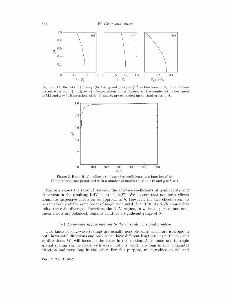
The numerical calculations of c1, c2 and c3 are performed using a Fourier spec-tral method. The Fourier multipliers involving β(x)Dx are consistently expanded upto third order in β, and explicit Fourier multiplier operations are performed usingfast Fourier transforms. Typically, we chose a number of modes equal to 512 andg = h = 1. Figure 1 shows graphs of the coefficients h + c1, 1 + c2 and 1

3h3 + c3.We note that all three coefficients decrease with increasing β0. The interpretationis that the time-scale describing the KdV regime is slower with increasing β0. Bet-ter approximations to c1, c2 and c3 can be obtained for β0 close to h by includinghigher-order terms, but this would not change qualitatively the results.



0.5 1.0 1.5

β0

0

0.2

0.4

0.6

0.8

1.0

h + c1−

0.5 1.0 1.501 + c2

−0.2 0.40

c3 + h3/ 3−

(a) (b) (c)

Figure 1. Coefficients (a) h + c1, (b) 1 + c2 and (c) c3 + 13h3 as functions of β0. The bottom

perturbation is β(x) = β0 cos(x). Computations are performed with a number of modes equalto 512 and h = 1. Expressions of c1, c2 and c3 are expanded up to third order in β.

100 200 300 400 500 6000

0.2

0.4

0.6

0.8

1.0

ratio

β0

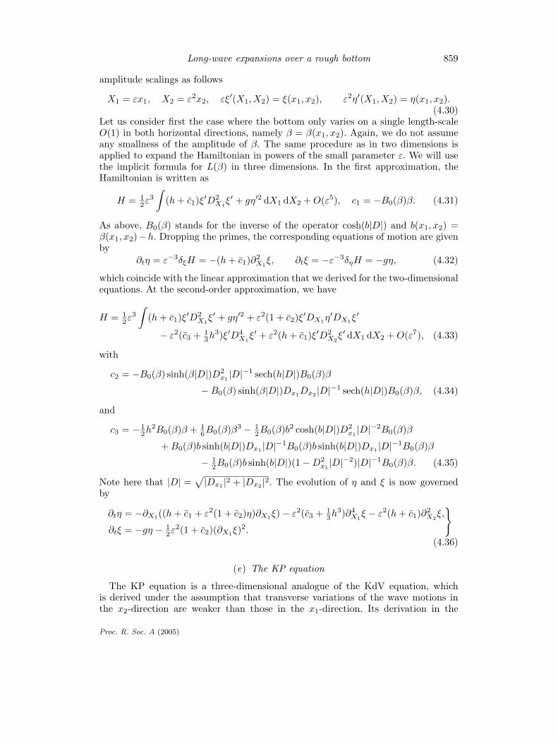
Figure 2. Ratio R of nonlinear to dispersive coefficients as a function of β0.Computations are performed with a number of modes equal to 512 and g = h = 1.

Figure 2 shows the ratio R between the effective coefficients of nonlinearity anddispersion in the resulting KdV equation (4.27). We observe that nonlinear effectsdominate dispersive effects as β0 approaches h. However, the two effects seem tobe remarkably of the same order of magnitude until β0 � 0.7h. As β0/h approachesunity, the ratio diverges. Therefore, the KdV regime, in which dispersive and non-linear effects are balanced, remains valid for a significant range of β0.

(d) Long-wave approximation to the three-dimensional problem

Two kinds of long-wave scalings are usually possible: ones which are isotropic inboth horizontal directions and ones which have different length-scales in the x1- andx2-directions. We will focus on the latter in this section. A common non-isotropicspatial scaling regime deals with wave motions which are long in one horizontaldirection and very long in the other. For this purpose, we introduce spatial and



amplitude scalings as follows

X1 = εx1, X2 = ε2x2, εξ′(X1, X2) = ξ(x1, x2), ε2η′(X1, X2) = η(x1, x2).(4.30)

Let us consider first the case where the bottom only varies on a single length-scaleO(1) in both horizontal directions, namely β = β(x1, x2). Again, we do not assumeany smallness of the amplitude of β. The same procedure as in two dimensions isapplied to expand the Hamiltonian in powers of the small parameter ε. We will usethe implicit formula for L(β) in three dimensions. In the first approximation, theHamiltonian is written as

H = 12ε3

∫(h + c1)ξ′D2

X1ξ′ + gη′2 dX1 dX2 + O(ε5), c1 = −B0(β)β. (4.31)

As above, B0(β) stands for the inverse of the operator cosh(b|D|) and b(x1, x2) =β(x1, x2)−h. Dropping the primes, the corresponding equations of motion are givenby

∂tη = ε−3δξH = −(h + c1)∂2X1

ξ, ∂tξ = −ε−3δηH = −gη, (4.32)

which coincide with the linear approximation that we derived for the two-dimensionalequations. At the second-order approximation, we have

H = 12ε3

∫(h + c1)ξ′D2

X1ξ′ + gη′2 + ε2(1 + c2)ξ′DX1η

′DX1ξ′

− ε2(c3 + 13h3)ξ′D4

X1ξ′ + ε2(h + c1)ξ′D2

X2ξ′ dX1 dX2 + O(ε7), (4.33)

with

c2 = −B0(β) sinh(β|D|)D2x1

|D|−1 sech(h|D|)B0(β)β

− B0(β) sinh(β|D|)Dx1Dx2 |D|−1 sech(h|D|)B0(β)β, (4.34)

and

c3 = −12h2B0(β)β + 1

6B0(β)β3 − 12B0(β)b2 cosh(b|D|)D2

x1|D|−2B0(β)β

+ B0(β)b sinh(b|D|)Dx1 |D|−1B0(β)b sinh(b|D|)Dx1 |D|−1B0(β)β

− 12B0(β)b sinh(b|D|)(1 − D2

x1|D|−2)|D|−1B0(β)β. (4.35)

Note here that |D| =√

|Dx1 |2 + |Dx2 |2. The evolution of η and ξ is now governedby

∂tη = −∂X1((h + c1 + ε2(1 + c2)η)∂X1ξ) − ε2(c3 + 13h3)∂4

X1ξ − ε2(h + c1)∂2

X2ξ,

∂tξ = −gη − 12ε2(1 + c2)(∂X1ξ)

2.

}

(4.36)

(e) The KP equation

The KP equation is a three-dimensional analogue of the KdV equation, whichis derived under the assumption that transverse variations of the wave motions inthe x2-direction are weaker than those in the x1-direction. Its derivation in the



present Hamiltonian framework is carried out by means of the same technique asthat described in § 4 b. Let us express the Hamiltonian (4.33) in terms of u′ = ∂X1ξ

′:

H = 12ε3

∫(h + c1)u′2 + gη′2 + ε2(1 + c2)η′u′2

− ε2(c3 + 13h3)(∂X1u

′)2 + ε2(h + c1)(∂−1X1

∂X2u′)2 dX1 dX2 + O(ε7). (4.37)

Making the further change of variables

η′ = 4

√(h + c1)

4g(r + s), u′ = 4

√g

4(h + c1)(r − s), (4.38)

one arrives at

H = 12ε3

∫ √g(h + c1)(r2 + s2) + 1

2ε2(1 + c2) 4

√g

4(h + c1)(r3 − r2s − rs2 + s3)

− ε2(c3 + 13h3)

√g

4(h + c1)(∂X1(r − s))2

+ 12ε2(h + c1)

√g

h + c1(∂−1

X1∂X2(r − s))2 dX1 dX2. (4.39)

Subtracting the momentum integral (4.22) and restricting the phase space to an ε2-neighbourhood of η ∼ u as in the two-dimensional case, the Hamiltonian reduces to

H − c0I = 12ε3

∫12ε2(1 + c2) 4

√g

4(h + c1)r3 − ε2(c3 + 1

3h3)√

g

4(h + c1)(∂X1r)

2

+ 12ε2(h + c1)

√g

h + c1(∂−1

X1∂X2r)

2 dX1 dX2, (4.40)

which is valid up to O(ε5). One can write a system of equations for r and s, in termsof a slow time variable T = ε2t, as

∂T r = −ε−5∂X1δr(H − c0I) = −32(1 + c2) 4

√g

4(h + c1)r∂X1r

− (c3 + 13h3)

√g

4(h + c1)∂3

X1r − (h + c1)

√g

h + c1∂−1

X1(∂2

X2r), (4.41)

and

∂T s = ε−5∂X1δs(H − c0I) = 0, (4.42)

which is accurate up to terms of O(ε2). Equation (4.41) corresponds to the KPequation for a rapidly varying bottom topography in three dimensions, while equa-tion (4.42) implies that in the present approximation there is no change in s, at leastover time-intervals T ∈ [−T0(ε), T0(ε)], with T0(ε) = O(ε−2).

5. Bottom topography with multiple spatial scales

(a) The two-dimensional Boussinesq regime

We consider the Boussinesq scaling (4.1) but now allow the bottom to vary bothon a length-scale O(1) and on a slowly varying scale, namely β = β(x, X), where



X = εx. Again, no assumption is made on the amplitude of β. It also may bepossible that more than one slow scale behaviour is present, whereupon we writeβ = β(x, X; ε). We will make explicit the behaviour of multiple scales. As before,the effort in the asymptotic expansion is almost entirely in examining the Dirichlet–Neumann operator, giving the result that

DL(β) = −εDxB0(β)βDX

− ε2DXB0(β)βDX + ε2DxB0(β)b sinh(bDx)DXB0(β)βDX

+ ε3 12h2DxB0(β)βD3

X − ε3 16DxB0(β)β3D3

X

+ ε3 12DxB0(β)b2 cosh(bDx)D2

XB0(β)βDX

+ ε3DXB0(β)b sinh(bDx)DXB0(β)βDX

− ε3DxB0(β)b sinh(bDx)DXB0(β)b sinh(bDx)DXB0(β)βDX

+ ε4 12h2DXB0(β)βD3

X − ε4 16DXB0(β)β3D3

X

+ ε4 12DXB0(β)b2 cosh(bDx)D2

XB0(β)βDX

− ε4 12h2DxB0(β)b sinh(bDx)DXB0(β)βD3

X

+ ε4 16DxB0(β)b sinh(bDx)DXB0(β)β3D3

X

+ ε4 16DxB0(β)b3 sinh(bDx)D3

XB0(β)βDX

− ε4 12DxB0(β)b sinh(bDx)DXB0(β)b2 cosh(bDx)D2

XB0(β)βDX

− ε4 12DxB0(β)b2 cosh(bDx)D2

XB0(β)b sinh(bDx)DXB0(β)βDX

− ε4DXB0(β)b sinh(bDx)DXB0(β)b sinh(bDx)DXB0(β)βDX

+ ε4DxB0(β)b sinh(bDx)DXB0(β)b sinh(bDx)

× DXB0(β)b sinh(bDx)DXB0(β)βDX + O(ε5), (5.1)

in the resulting expansion of G(0) in (4.3), and in the expansion of the term G(1)

in (4.4), one finds that

D tanh(hD)ηDL(β) = −ε3D2x tanh(hDx)B0(β)βη′(X)DX

+ ε4D2x tanh(hDx)B0(β)b sinh(bDx)η′(X)DXB0(β)βDX

− ε4Dx tanh(hDx)η′(X)DXB0(β)βDX

− ε4hD2x sech(hDx)2DXB0(β)βη′(X)DX

− ε4Dx tanh(hDx)DXB0(β)βη′(X)DX + O(ε5), (5.2)

and that

DL(β)ηDL(β) = ε3DxB0(β) sinh(βDx)Dx sech(hDx)B0(β)βη′(X)DX

− ε4DxB0(β) sinh(βDx)Dx sech(hDx)

× B0(β)b sinh(bDx)η′(X)DXB0(β)βDX

+ ε4DxB0(β) sinh(βDx) sech(hDx)η′(X)DXB0(β)βDX



− ε4hDxB0(β) sinh(βDx)Dx tanh(hDx)

× sech(hDx)DXη′(X)B0(β)βDX

+ ε4DxB0(β)β cosh(βDx)Dx sech(hDx)

× DXη′(X)B0(β)βDX

− ε4DxB0(β)b sinh(bDx)DXB0(β) sinh(βDx)

× Dx sech(hDx)B0(β)βη′(X)DX

+ ε4DXB0(β) sinh(βDx)Dx sech(hDx)

× B0(β)βη′(X)DX + O(ε5). (5.3)

For simplicity of notation, the quantities β and b are written without any independentvariables in (5.1)–(5.3), but recall that β = β(x, X) and b = b(x, X) = β(x, X) − hare functions of multiple spatial scales.

Retaining explicit calculations of terms of up to O(ε3), the Hamiltonian reads

1ε3 H = 1

2

∫−ε−1DxB0(β)βξ′(X)DXξ′(X) + gη′2(X)

− (1 − DxB0(β)b sinh(bDx))ξ′(X)DXB0(β)βDXξ′(X)

+ hξ′(X)D2Xξ′(X) dX + O(ε1). (5.4)

Again, the lemma of scale separation allows us to write

1ε3 H = 1

2

∫gη′2(X) − (h + c1(X))(DXξ′)2 dX + O(ε), (5.5)

where c1 = −B0(β)β. Dropping the primes, the corresponding equations of motionare given in terms of u = ∂Xξ by

∂tη = −∂X((h + c1)u), ∂tu = −g∂Xη. (5.6)

In this form, equations (5.6) only differ from (4.14) by the X-dependence of thecoefficient c1. Higher-order corrections can be derived in a similar way. Keepingterms up to O(ε5) in the Hamiltonian, we have

1ε3 H = 1

2

∫gη′2(X) − (h + c1(X))(DXξ′)2 − εc2(X)(DXξ′)2 − ε2c3(X)(DXξ′)2

+ ε2(c4(X) + 13h3)(DXξ′)D3

Xξ′ − ε2c5(X)(D2Xξ′)2

− ε2(1 + c6(X))η′(X)(DXξ′)2 dX + O(ε3), (5.7)

with

c2 = B0(β)b sinh(bDx)DX(B0(β)β) − 12DX(B0(β)b sinh(bDx)B0β), (5.8)

c3 = 12B0(β)b2 cosh(bDx)D2

X(B0(β)β)

+ DX(B0(β)b sinh(bDx))B0(β)b sinh(bDx)DX(B0(β)β)

− 12DX(B0(β)b2 cosh(bDx)DX(B0(β)β)

+ DX(B0(β)b sinh(bDx))B0(β)b sinh(bDx)B0(β)β+ B0(β)b sinh(bDx)B0(β)b sinh(bDx)DX(B0(β)β)), (5.9)



c4 = −12h2B0(β)β + 1

6B0(β)β3 − 12B0(β)b2β, (5.10)

c5 = B0(β)b sinh(bDx)B0(β)b sinh(bDx)B0(β)β, (5.11)

c6 = −B0(β) sinh(βDx)Dx sech(hDx)B0(β)β. (5.12)

The equations of motion given by this approximation are

∂tη = −∂X((h(X) + ε2(1 + c6)η)u) − ε2∂2X((1

3h3 + c4 + c5)∂Xu),

∂tu = −g∂Xη − 12ε2∂X((1 + c6)u2).

}(5.13)

where the effective depth is expressed by h(X) = h + c1 + εc2 + ε2c3 + 12ε2(∂2

X c4).Recall that the coefficients ci are X-dependent. One can see that the presence of

a slowly varying bottom topography introduces additional dispersive and nonlinearterms in the evolution equation of η. It can be seen from the form of the terms ofO(ε5) in the expansion of the rescaled Dirichlet–Neumann operator (5.1) that thereare non-zero terms in the approximate Hamiltonian (5.7) of O(ε6), and therefore thetime-interval of validity of these equations is less than in the case of a bottom withno variations on a slow spatial scale. The most pessimistic view states that the errorterms implied in the approximate long-wave equations (5.13) are of O(ε3), and there-fore it affords the possibility that over time-intervals longer than T (ε) = o(ε−1) theerror can grow to compete with the terms retained in the system of equations (5.13).

(b) The three-dimensional Boussinesq regime

In the three-dimensional situation, in cases where the bottom varies both ona length-scale O(1) and on a slowly varying scale in both horizontal directions(i.e. β = β(x1, X1, x2, X2)), we find up to O(ε3) and O(ε5), respectively, that

H = 12ε3

∫gη′2 − (h + c1)(DX1ξ

′)2 dX1 dX2 + O(ε4), (5.14)

where c1 = −B0(β)β and

H = 12ε3

∫gη′2 − (h + c1)(DX1ξ

′)2 − εc2(DX1ξ′)2

− ε2c3(DX1ξ′)2 + ε2(c4 + 1

3h3)(DX1ξ′)D3

X1ξ′ − ε2c5(D2

X1ξ′)2

− ε2(1 + c6)η′(DX1ξ′)2 − ε2(h + c1)(DX2ξ

′)2

+ ε2c7(DX1ξ′)(DX1DX2ξ

′) dX1 dX2 + O(ε6), (5.15)

with

c2 = B0(β)b sinh(b|D|)Dx1 |D|−1DX1(B0(β)β)

− 12DX1(B0(β)b sinh(b|D|)Dx1 |D|−1B0β), (5.16)

c3 = DX1(B0(β)b sinh(b|D|))Dx1 |D|−1B0(β)b sinh(b|D|)Dx1 |D|−1DX1(B0(β)β)

+ 12B0(β)b2 cosh(b|D|)D2

x1|D|−2D2

X1(B0(β)β)

+ 12B0(β)b sinh(b|D|)(1 − D2

x1|D|−2)|D|−1D2

X1(B0(β)β)

+ B0(β)b sinh(b|D|)Dx2 |D|−1DX2(B0(β)β)

− 12DX1(B0(β)b2 cosh(b|D|)D2

x1|D|−2DX1(B0(β)β)



+ B0(β)b sinh(b|D|)(1 − D2x1

|D|−2)|D|−1DX1(B0(β)β)

+ DX1(B0(β)b sinh(b|D|))Dx1 |D|−1B0(β)

× b sinh(b|D|)Dx1 |D|−1B0(β)β

+ B0(β)b sinh(b|D|)Dx1 |D|−1B0(β)

× b sinh(b|D|)Dx1 |D|−1DX1(B0(β)β)), (5.17)

c4 = −12h2B0(β)β + 1

6B0(β)β3 − 12B0(β)b2 cosh(b|D|)D2

x1|D|−2B0(β)β

− 12B0(β)b sinh(b|D|)(1 − D2

x1|D|−2)|D|−1B0(β)β, (5.18)

c5 = B0(β)b sinh(b|D|)Dx1 |D|−1B0(β)b sinh(b|D|)Dx1 |D|−1B0(β)β, (5.19)

c6 = −B0(β) sinh(β|D|)D2x1

|D|−1 sech(h|D|)B0(β)β

− B0(β) sinh(β|D|)Dx1Dx2 |D|−1 sech(h|D|)B0(β)β, (5.20)

c7 = −iB0(β)b sinh(b|D|)Dx2 |D|−1B0(β)β. (5.21)

The corresponding approximate equations of motion to lowest order are

∂tη = −∂X1((h(X1, X2) + ε2(1 + c6)η)∂X1ξ)

− ε2∂2X1

((c4 + 13h3 + c5)∂2

X1ξ) − ε2∂X2((h + c1)∂X2ξ),

∂tξ = −gη − 12ε2(1 + c6)(∂X1ξ)

2, (5.22)

where the effective depth in this situation is given by the expression

h = h + c1 + εc2 + ε2c3 + 12ε2(∂2

X1c4) − 1

2ε2(∂X2 c7).

Recall that all coefficients ci depend on X1 and X2.

(c) Unidirectional equations in a regime with multiple spatial scales

In order to derive a unidirectional equation in the Boussinesq regime with multiplespatial scales, we extend our analysis by considering the more general case whereβ = β(x, X; ε). The equations of motion consist of a system of coupled equations forthe right- and left-moving components. The coupling at first order, which determinesthe role of wave scattering, is measured by the slope of the effective depth in theproblem. Two typical examples of multiscale dependence for the bottom are

β = β(x, X), X = εαX = εα+1x, (5.23)

β = β0(x) + εγβ1(x, X), X = εδX = εδ+1x, (5.24)

where α, γ, δ � 0. The parameters α in (5.23) and γ + δ in (5.24) provide a measurefor the steepness of the slowly varying bottom. This is the regime in which thebottom perturbation varies over an even longer length-scale than the wave motionrepresented by η(X) and ξ(X). To illustrate the problem, we will present the analysisonly in the case (5.23), which was also considered by van Groesen & Pudjaprasetya(1993).



At the second order of approximation, the Hamiltonian (5.7) is given by

H = 12ε3

∫gη′(X)2 + (h + c1(X) + εα+1c2(X) + ε2α+2c3(X)

+ 12ε2α+2(∂2

Xc4(X)))u′(X)2

− ε2(13h3 + c4(X) + c5(X))(∂Xu′(X))2

+ ε2(1 + c6(X))η′(X)u′(X)2 dX + O(ε5+α). (5.25)

Making the change of variables

η′ = 4

√h(X)4g

(r + s), u′ = 4

√g

4h(X)(r − s), (5.26)

where the effective depth h is

h(X) = h + c1(X) + εα+1c2(X) + ε2α+2c3(X) + 12ε2α+2∂2

Xc4(X), (5.27)

the Hamiltonian becomes

H = 12ε3

∫ √gh(r2 + s2) − ε2(1

3h3 + c4 + c5)

×[(

4

√g

4h∂Xr

)2

− 2(

4

√g

4h∂Xr

)(4

√g

4h∂Xs

)+

(4

√g

4h∂Xs

)2]

+ ε2(

1 + c6

2

)4

√g

4h(r3 − r2s − rs2 + s3) dX + o(ε5). (5.28)

The evolution equations for r and s are now written as

∂t

(rs

)=

1ε3

( −∂X14εα(∂X log(h))

−14εα(∂X log(h)) ∂X

) (δrHδsH

). (5.29)

The solutions r and s correspond to predominantly right- and left-moving wavemotions, respectively. The presence of the non-diagonal terms 1

4εα∂X log(h(X))in (5.29) is a consequence of the bottom variations and gives rise to the effect ofwave scattering. Note that, unlike the case of a rapidly varying bottom topography,we do not subtract the momentum integral from the Hamiltonian in order to trans-form to a moving reference frame, since momentum is not a conserved quantity whenthe depth is variable.

In case that α = 0, the result (5.29) is the following system of two coupled KdV-likeequations:

∂tr = −∂X(C0(X)r + ε2∂X(C1(X)(∂Xr − ∂Xs)) + ε2C2(X)(3r2 − 2rs − s2))

+ S(X)(C0(X)s − ε2∂X(C1(X)(∂Xr − ∂Xs)) + ε2C2(X)(−r2 − 2rs + 3s2)),(5.30)

∂ts = ∂X(C0(X)s − ε2∂X(C1(X)(∂Xr − ∂Xs)) + ε2C2(X)(−r2 − 2rs + 3s2))

− S(X)(C0(X)r + ε2∂X(C1(X)(∂Xr − ∂Xs)) + ε2C2(X)(3r2 − 2rs − s2)).(5.31)



The coefficients are defined as

C0(X) =√

gh(X), C1(X) = (13h3 + c4 + c5)

√g

4h,

C2(X) = 14(1 + c6) 4

√g

4h, S(X) = 1

4(∂X log(h)).

In (5.30) and (5.31), the expression for the effective linear phase speed is C0(X);we note that this includes higher-order terms in ε. Because of the strong couplingbetween the wave fields r(X, t) and s(X, t), these two do not separate into indepen-dent solutions for a unidirectional regime.

When α > 0, and when the initial data r0(X) and s0(X) are functions which arelocalized spatially, the analysis divides into several cases.

(i) Case 1

When α � 2, corresponding to very mild slopes, and initial conditions s0 = O(ε2),one rescales s = ε2s′ and r = r′ in equations (5.30), (5.31). Dropping terms of higherorder, we have

∂tr′ = −∂X(C0(X)r′ + ε2(∂X(C1(X)∂Xr′) + 3C2(X)r′2)),

∂ts′ = ∂X(C0(X)s′ − ∂X(C1(X)∂Xr′) − C2(X)r′2) − εα−2S(X)C0(X)r′.

}(5.32)

This system consists of an equation in closed form for r′(X, t), which is a KdVequation with slowly varying coefficients representing a principally right-moving wavefield, and a second equation for a reflected wave s′(X, t). The solution s′(X, t) isrecovered from r′(X, t) by quadrature along left-moving characteristics, defined byX = −C0(X).

This system of equations describing r′(X, t) is a valid asymptotic regime at leastover time-intervals of order T (ε) = o(ε−1), the same time-interval as for the Boussi-nesq system (5.13), but a strictly shorter time-interval than the case of the KdVequation with constant coefficients (as arising with a flat or a rapidly varying bot-tom without slow spatial variations). This is due in part to the nature of the errorfrom truncation of the Hamiltonian. Furthermore, over such time-intervals the scat-tering component s′(X, t) remains bounded. This latter fact is true because initialconditions r′

0(X) which is spatially localized (that is, essentially supported in a neigh-bourhood of diameter O(1)) gives rise to solutions r′(X, t) which move essentiallyto the right. The quadrature for the scattering component s′(X, t) is along left-moving characteristics, which encounter regions in which r′(X, t) is of significantamplitude only over intervals of length O(1). Therefore, s′(X, t) does not grow by anamount larger than O(1), even for quadrature over long time-intervals, as much asT (ε) = o(ε−1). This will not be the case over longer intervals, for initial conditionswhich is not spatially localized, for instance in case the initial conditions are periodic.

(ii) Case 2

When 32 � α < 2 and the initial conditions satisfy s0 = O(εα), we obtain equations

for r(X, t) = r′(X, t) and s(X, t) = εαs′(X, t), which are again in the form of a KdV



equation coupled to an equation for the left-moving scattered field:

∂tr′ = −∂X(C0(X)r′ + ε2(∂X(C1(X)∂Xr′) + 3C2(X)r′2)), (5.33)

∂ts′ = ∂X(C0(X)s′ − ε2−α∂X(C1(X)∂Xr′) − ε2−αC2(X)r′2) − S(X)C0(X)r′.

(5.34)

Equation (5.33) is a KdV equation in r with variable coefficients. The evolutionof the reflected component of the solution s′(X, t) is governed by (5.34). From thescaling, it is proportional to the slope of the bottom. As in the previous case, thisscaling regime is valid for time-intervals of order T (ε) = o(ε−1).

(iii) Case 3

When 1 < α < 32 and the initial conditions satisfy s0 = O(εα), the system of equa-

tions describing r′(X, t) is still given by (5.33), but the error in truncation is poten-tially larger, and the time-interval in which one is assured of the validity of theapproximation is shorter, namely T (ε) = o(ε2(1−α)).

(iv) Case 4

If α = 1, the basic equation for the right-moving component r′(X, t) is modifiedby a coupling term to the reflected component. The appropriate scaling is r(X, t) =r′(X, t) and s(X, t) = εs′(X, t), giving rise to the system of equations

∂tr′ = −∂X(C0(X)r′ + ε2(∂X(C1(X)∂Xr′) + 3C2(X)r′2)) + ε2S(X)C0(X)s′,

∂ts′ = ∂X(C0(X)s′) − S(X)C0(X)r′.

}

(5.35)The scaling regime gives a valid approximation for both r′(X, t) and s′(X, t), fortime-intervals of order T (ε) = o(ε−1) as in case 1; it is of this length because ofthe increased accuracy given by inclusion of the extra coupling term, although wesacrifice the simplicity of a decoupled equation for r′(X, t). We also note that becauseof the coarser scaling in s′ the permissible error is greater.

(v) Case 5

Finally, if 0 < α � 1, the evolutions of r′ = r and εαs′ = s decouple only weakly,and over time-intervals of O(ε−2α). A coarse description of the evolution is given by

∂tr′ = −∂X(C0(X)r′),

∂ts′ = ∂X(C0(X)s′) − S(X)C0(X)r′,

}(5.36)

where the error of truncation is O(ε2α). Dispersion in the right-moving component isnot as significant as scattering effects in this linear system, and therefore dispersiveterms have been eliminated. Returning to the case α = 0 corresponds to the fullycoupled system (5.30), (5.31).

Similar results can be obtained for a bottom topography of the form (5.24). Inparticular, the case γ = 2, δ = 0 was examined by Whitham (1974). It should benoted that KdV-type equations for a slowly varying bottom in this setting have also



been derived by several other authors, including Johnson (1973), Miles (1979) andNewell (1985).

The present analysis can be extended to three dimensions in a straightforwardmanner. For brevity, we will only give one example. Assuming that the wave motionis primarily one-dimensional in the x1-direction and that the bottom has the followingdependence

β = β(x1, X1, x2, X2), (5.37)

where X1 = εαX1 = εα+1x1 and X2 = ε2αX2 = ε2α+2x2, a three-dimensional ana-logue of (5.32), for α � 2 can be derived as

∂tr = −√

gh∂X1r − ε2√

g

4h(c4 + 1

3h3 + c5)∂3X1

r

− 3ε2 4

√g

4h12(1 + c6)r∂X1r − ε2

√g

4h(h + c1)∂−1

X1(∂2

X2r), (5.38)

with h redefined as

h(X1, X2) = h + c1 + εα+1c2 + ε2α+2c3 + 12ε2α+2∂2

X1c4 − 1

2ε2α+2∂X2c7. (5.39)

Equation (5.38) can be viewed as the KP equation with slowly varying coefficientsfor very mild slopes of the bottom.

6. Conclusions

We study the long-wave asymptotic regime for water waves in a fluid domain ofvariable depth as a perturbation problem for a Hamiltonian system depending on asmall parameter. The formulation of the problem in terms of Zakharov’s Hamilto-nian, using an expression for the Dirichlet integral in terms of the Dirichlet–Neumannoperator, is convenient for the analysis. When the bottom varies periodically on ashort length-scale, the motion of long-wavelength solutions is essentially governed bya system related to the Boussinesq equation, whose effective coefficients are deter-mined by homogenization averages. In a regime emphasizing one-way propagation,the same conclusion holds for solutions of a KdV equation. Similar results hold in thethree-dimensional case, where bi-directional long-wavelength motions are governedby a Boussinesq-like system, and one-way motions by a system closely related to theKP equations. Expressions for the coefficients are quite explicit, and typical casesare computed numerically. We find the following results.

(i) The linear wave speed of the long waves is slower for non-constant bottomvariations than for that of a flat bottom with the same average depth. Thisrecovers the result of Rosales & Papanicolaou (1983) in two dimensions for aperiodic bottom.

(ii) For bottom variations with fixed average depth, but which approach the shoal-ing limit, the effective coefficient of the nonlinear term dominates the effectivecoefficients of dispersive terms in the KdV equation. However, this is significantonly for very large variations, and over a large range of bottom perturbationsthe nonlinearity and the dispersive effects are quite well balanced. This servesto justify the use of the Boussinesq and KdV equations for a wide range ofbottom topography.



(iii) The time-scale of the effects of both nonlinearity and dispersion are significantlyslower for large amplitude variations of the bottom (always considering theaverage depth fixed).

In cases in which the periodic variations of the bottom themselves vary on the longlength-scale, we derive a number of Hamiltonian PDEs with variable coefficients todescribe the evolution of surface waves. Because of the presence of the variations inthe bottom, there are additional terms in the long-wave equations. Even at the lowestorder in perturbation theory, terms are present which describe the linear effect ofreflection of waves by the bottom topography. Denoting the effective depth by h(X),we show that the linear reflection from left-propagating to right-propagating modes(and vice versa) is proportional to S = ∂X log(h). This coefficient depends uponX = εx, as do the resulting effective coefficients of dispersion and nonlinearity; itappears both in the two-dimensional Boussinesq system and in its three-dimensionalanalogue.

In the general case, the quantity S(X) is of O(1), and it does not make sense toseek special solutions whose motions are principally unidirectional; any such solutiongenerates a substantial reflection in an O(1) length of time. However, in cases inwhich S = S(X; ε) also depends upon the scaling parameter ε, such as when thelong-wavelength variations are small amplitude, or have small slope, or both, then∂X h(X; ε) ∼ O(εα), and it is possible to proceed further. Depending on the value ofα, we find five different regimes that can be described in detail.

Finally, we would like to point out that the formulation of the Dirichlet–Neumannoperator as given in this paper is suitable for the numerical simulation of the full equa-tions of the water wave problem with bottom topography. The recursive expressionsin terms of Fourier multipliers and of surface/bottom variations can be numericallyevaluated using a spectral method with fast Fourier transforms. Preliminary numer-ical results appear in Guyenne & Nicholls (2004). More in-depth numerical compu-tations constitute a substantial contribution in their own right, and are beyond thescope of the present paper. These are envisioned for a separate and distinct article.

Appendix A. Taylor expansions of G(β, η) and L(β)

In § 2 b, we give a Taylor expansion of the Dirichlet–Neumann operator G(β, η) inpowers of η. The recursion formula for G(β, η) is found to be the same as that for thecase of a flat bottom, with the operator L(β) being absorbed in the lowest-order termG(0) of the recursion formula. Here we present an alternative formulation for G(β, η)as a double series in both β and η. This requires in particular a Taylor expansion ofL(β) in powers of β.

Consider the Dirichlet–Neumann operator in the form G(β, η) =∑

j,l Gj,l(β, η),where the Gj,l are homogeneous of degree j and l in powers of β and η, respectively.The terms G0,l identify with the terms in the expansion of the Dirichlet–Neumannoperator for a flat bottom. It is convenient to compute the coefficients Gj,0 whichcorrespond to a domain with a flat interface and a variable bottom topography.For this purpose, let us consider the problem (2.6) with η = 0. Its solution can beexpressed in the form of (2.9). By the definition of G, we have

G(β, 0)ξ ≡ ∂yϕ(x, 0) = D tanh(hD)ξ + DL(β)ξ. (A 1)



Equivalently,

G0,0 = D tanh(hD), Gj,0 = D tanh(hD) + DLj(β), (A 2)

where the Lj(β) are the terms in the expansion of L(β) in powers of β. To computethem explicitly, we write the Neumann condition at y = −h + β(x),

(∂yϕ − ∂xβ∂xϕ)(x,−h + β) = 0, (A 3)

and expand the various terms in powers of β.From the expression (2.9) for the function ϕ(x, y) one calculates its derivatives.

We now formally perform the Taylor expansions of the operators

D sinh((h + y)D)|y=−h+β =∑l odd

βl

l!Dl+1,

D cosh((h + y)D)|y=−h+β =∑

l even

βl

l!Dl+1,

D sinh(yD)|y=−h+β =∑

l even

βl

l!(−D)l+1 sinh(hD)

+∑l odd

βl

l!(−D)l+1 cosh(hD),

D cosh(yD)|y=−h+β =∑

l even

βl

l!Dl+1 cosh(hD) −

∑l odd

βl

l!Dl+1 sinh(hD).

⎫⎪⎪⎪⎪⎪⎪⎪⎪⎪⎪⎪⎪⎪⎪⎪⎪⎪⎪⎪⎬⎪⎪⎪⎪⎪⎪⎪⎪⎪⎪⎪⎪⎪⎪⎪⎪⎪⎪⎪⎭(A 4)

It is important to notice that in the above expansions, the operator D does not acton β. Equation (A 3) is now rewritten as

∑l odd

βl

l!sech(hD)Dl+1 +

∑l even

βl

l!cosh(hD)L(β) −

∑l odd

βl

l!sinh(hD)L(β)

− i(∂xβ)(

βl

l!sech(hD)Dl+1 +

∑l odd

βl

l!cosh(hD)L(β)

−∑

l even

βl

l!Dl+1 sinh(hD)L(β)

)= 0. (A 5)

Identification of the terms in zero, first and second powers of β leads to

L0 = 0, L1 = − sech(hD)β sech(hD), L2 = sech(hD)βD sinh(hD)L1.

More generally, the recursion formula takes the form:

Lj = − sech(hD)[βj

j!sech(hD)Dj +

j−1∑l=2,even

βl

l!Dl cosh(hD)Lj−l

−j−2∑

l=1,odd

βl

l!Dl sinh(hD)Lj−l

](A 6)



for j odd and

Lj = − sech(hD)[ j−2∑

l=2,even

βl

l!Dl cosh(hD)Lj−l −

j−1∑l=1,odd

βl

l!Dl sinh(hD)Lj−l

](A 7)

for j > 0 even.

We point out that the recursion formula given in (A 6) and (A 7) can be directlyobtained by a Taylor expansion of the implicit formula for L(β) in powers of β.

The recursion formula of L(β) can be easily extended to three dimensions, takingthe form:

Lj = − D

|D| sech(h|D|)

·[βj

j!sech(h|D|)|D|j−1D +

j−1∑l=2,even

βl

l!cosh(h|D|)|D|l−1DLj−l

−j−2∑

l=1,odd

βl

l!sinh(h|D|)|D|l−1DLj−l

], (A 8)

for j odd and

Lj = − D

|D| sech(h|D|) ·[ j−2∑

l=2,even

βl

l!cosh(h|D|)|D|l−1DLj−l

−j−1∑

l=1,odd

βl

l!sinh(h|D|)|D|l−1DLj−l

]. (A 9)

for j > 0 even.Putting together the expansions of L(β) in powers of β above and the expansions

of G(β, η) in terms of L(β) and powers of η as given in § 2 c, one obtains an expressionfor the series expansion of the Dirichlet–Neumann operator as a double series in β(x)and η(x). Using the fact that G(β, η) is self-adjoint, one can write, for any j > 0 andl > 0 even,

Gj,l = Lj |D|l−1D · ηl

l!D

−l−2∑

p=0,even

|D|l−p ηl−p

(l − p)!Gj,p

−l−1∑

p=1,odd

G0,0|D|l−p−1 ηl−p

(l − p)!Gj,p

−l−1∑

p=1,odd

j−1∑q=0

Lj−q|D|l−p ηl−p

(l − p)!Gq,p, (A 10)



and, for any j > 0 and l odd,

Gj,l = −l−2∑

p=1,odd

|D|l−p ηl−p

(l − p)!Gj,p

−l−1∑

p=0,even

G0,0|D|l−p−1 ηl−p

(l − p)!Gj,p

−l−1∑

p=0,even

j−1∑q=0

Lj−q|D|l−p ηl−p

(l − p)!Gq,p. (A 11)

The research of W.C. was partly supported by the Canada Research Chairs Program, the NSERCthrough grant no. 238452-01 and the NSF through grant no. DMS-0070218. Part of this workwas performed while W.C. was a member of the MSRI, Berkeley. The research of P.G. was partlysupported by a SHARCNET Postdoctoral Fellowship at McMaster University and the NSERCthrough grant no. 238452-01. The research of D.N. was partly supported by the NSF throughgrant nos DMS-0196452 and DMS-0139822. The research of C.S. was partly supported by theNSERC through grant no. OGP 0046179.

References

Bensoussan, A., Lions, J.-L. & Papanicolaou, G. 1978 Asymptotic analysis of periodic structures.Studies in Mathematics and Its Applications, vol. 5. Amsterdam: North-Holland.

Craig, W. 1985 An existence theory for water waves and the Boussinesq and Korteweg–de Vriesscaling limits. Commun. PDEs 8, 787–1003.

Craig, W. & Groves, M. 1994 Hamiltonian long-wave scaling limits of the water-wave problem.Wave Motion 19, 367–389.

Craig, W. & Nicholls, D. 2002 Traveling gravity water waves in two and three dimensions. Eur.J. Mech. B 21(6), 615–641.

Craig, W. & Sulem, C. 1993 Numerical simulation of gravity waves. J. Computat. Phys. 108,73–83.

Craig, W., Sulem, C. & Sulem, P.-L. 1992 Nonlinear modulation of gravity waves: a rigorousapproach. Nonlinearity 5, 497–552.

Craig, W., Schanz, U. & Sulem, C. 1997 The modulation regime of three-dimensional waterwaves and the Davey–Stewartson system. Annls Inst. H. Poincare 14, 615–667.

Craig, W., Guyenne, P. & Kalisch, H. 2004 Hamiltonian long wave expansions for free surfacesand interfaces. (Submitted.)

Guyenne, P. & Nicholls, D. 2004 Numerical simulation of solitary waves on plane slopes. Math.Comput. Simulat. (In the press.)

Johnson, R. S. 1973 On the development of a solitary wave moving over an uneven bottom.Proc. Camb. Phil. Soc. 73, 183–203.

Kirby, J. T. 1997 Nonlinear dispersive long waves in water of variable depth. In Gravity wavesin water of finite depth (ed. J. N. Hunt). Advances in Fluid Mechanics, vol. 10, pp. 55–125.Springer.

Liu, Y. & Yue, D. K. P. 1998 On generalized Bragg scattering of surface waves by bottom ripples.J. Fluid Mech. 356, 297–356.

Mei, C. C. & Liu, P. L.-F. 1993 Surface waves and coastal dynamics. A. Rev. Fluid Mech. 25,215–240.



Miles, J. W. 1979 On the Korteweg–de Vries equation for a gradually varying channel. J. FluidMech. 91, 181–190.

Nachbin, A. & Papanicolaou, G. 1992 Water waves in channels of rapidly varying depth. J. FluidMech. 241, 311–332.

Newell, A. C. 1985 Solitons in mathematics and physics. Philadelphia, PA: SIAM.Rosales, R. & Papanicolaou, G. 1983 Gravity waves in a channel with a rough bottom. Stud.

Appl. Math. 68, 89–102.Smith, R. 1998 An operator expansion formulation for nonlinear surface water waves over vari-

able depth. J. Fluid Mech. 363, 333–347.van Groesen, E. & Pudjaprasetya, S. R. 1993 Uni-directional waves over slowly varying bottom.

I. Derivation of KdV type equation. Wave Motion 18, 345–370.Whitham, G. B. 1974 Linear and nonlinear waves. Wiley.Yoon, S. B. & Liu, P. L.-F. 1994 A note on Hamiltonian for long water waves in varying depth.

Wave Motion 20, 359–370.Zakharov, V. E. 1968 Stability of periodic waves of finite amplitude on the surface of a deep

fluid. J. Appl. Mech. Tech. Phys. 9, 1990–1994.

As this paper exceeds the maximum length normally permitted,the authors have agreed to contribute to production costs.


Documents

Hamiltonian long-wave expansions for water waves over a