Hamiltonian Hopf bifurcations and dynamics of NLS/GP standing-wave modes

This article has been downloaded from IOPscience. Please scroll down to see the full text article.

2011 J. Phys. A: Math. Theor. 44 425101

(http://iopscience.iop.org/1751-8121/44/42/425101)

Download details:

IP Address: 24.42.74.156

The article was downloaded on 01/10/2011 at 02:09

Please note that terms and conditions apply.

View the table of contents for this issue, or go to the journal homepage for more

Home Search Collections Journals About Contact us My IOPscience

IOP PUBLISHING JOURNAL OF PHYSICS A: MATHEMATICAL AND THEORETICAL

J. Phys. A: Math. Theor. 44 (2011) 425101 (28pp) doi:10.1088/1751-8113/44/42/425101

Hamiltonian Hopf bifurcations and dynamics ofNLS/GP standing-wave modes

Roy Goodman

Department of Mathematical Sciences, New Jersey Institute of Technology, Newark, NJ 07102,USA

E-mail: goodman@njit.edu

Received 31 January 2011, in final form 25 August 2011Published 30 September 2011Online at stacks.iop.org/JPhysA/44/425101

AbstractWe examine the dynamics of solutions to nonlinear Schrodinger/Gross–Pitaevskii equations that arise due to semisimple indefinite Hamiltonian Hopfbifurcations—the collision of pairs of eigenvalues on the imaginary axis. Weconstruct localized potentials for this model which lead to such bifurcations in apredictable manner. We perform a formal reduction from the partial differentialequations to a small system of ordinary differential equations. We analyzethe equations to derive conditions for this bifurcation and use averaging toexplain certain features of the dynamics that we observe numerically. A seriesof careful numerical experiments are used to demonstrate the phenomenon andthe relations between the full system and the derived approximations.

PACS numbers: 05.45.Ac, 02.30.Oz, 42.65.Sf, 42.65.Wi, 67.85.Hj

S Online supplementary data available from stacks.iop.org/JPhysA/44/425101/mmedia

(Some figures may appear in colour only in the online journal)

1. Introduction

This paper brings together several threads in the study of nonlinear waves in media with alocalized defect. It focuses on one specific example: the dynamics of low-amplitude solutionsto the nonlinear Schrodinger/Gross–Pitaevskii (NLS/GP) equation

i∂tu = Hu − |u|2u; H = −∂2x + V (x), (1.1)

in the presence of an oscillatory instability, arising from a particular type of Hamiltonian Hopf(HH) bifurcation. Our interest in this problem has four primary motivations. In the remainderof this section, we discuss these motivations, while simultaneously defining the mathematicalproblem to be studied.

1751-8113/11/425101+28$33.00 © 2011 IOP Publishing Ltd Printed in the UK & the USA 1

J. Phys. A: Math. Theor. 44 (2011) 425101 R Goodman

1.1. Physical motivation

In nonlinear optics, equation (1.1) describes the evolution of the envelope u(x, t) of anelectromagnetic field E inside a nonlinear waveguide [1, 2]. The equation is derived using theparaxial approximation, so that t measures the propagation distance along the waveguide axis,and x the transverse profile. The waveguide is assumed to be thin in the third (y) direction,so that variation in this direction can be safely ignored. The potential V (x) represents thewaveguide structure. The material is assumed to be Kerr nonlinear, i.e. a nonzero electric fieldE locally and quadratically modifies the refractive index, n = n0 + n2(|E|2).

When the sign on the nonlinear term of (1.1) is reversed, it describes the evolution of aBose–Einstein condensate (BEC), a state of matter achievable at extreme low temperatures inwhich atoms lose their individual identities and are described by a common wavefunction [3].For equation (1.1) to hold, the three-dimensional condensate must be strongly confined by asteep potential in the two transverse directions y and z so that it assumes a ‘cigar’ shape. Theterm V (x) then describes a less steeply confining potential in the third spatial dimension.

1.2. Mathematical motivation—moving from stability to dynamics

A fundamental object of study for systems like (1.1) is a nonlinear standing wave or boundstate, i.e. a localized solution to (1.1) of the form

u(x, t) = e−i�tU (x).

A solution consists of a function U (x) ∈ H2, and real numbers � and N satisfying�U = HU − U3;∫ ∞

−∞U2(x) dx = ||U ||22 = N .

(1.2)

The parameter N > 0 represents the number of particles of a BEC or the total intensity ofthe light in optics. This solution is a nonlinear generalization of an eigenfunction of a linearSchrodinger equation, although the principle of superposition does not apply. There existcontinuous families of solutions to (1.2) that are indexed by the intensity N . Some of thesefamilies persist in the limit N → 0, and approach the eigenpairs of the linear system. Wedenote the nonlinear continuation of the linear eigenfunction Uj(x) as UN

j (x).Nonlinear bound states, or standing waves, represent coherent and simple states that should

be observable in a laboratory experiment. Such bound states may be found numerically, or,for certain potentials V (x), computed exactly in the linear limit and perturbatively for N � 1.For such states to be observable in experiments, they must be stable, i.e. if a solution toequation (1.1) is initialized at t = 0 with value close to, but not equal to, a solution to system(1.2), then it must stay in a neighborhood of that solution for all t > 0.

The stability of such solutions has been widely studied, especially their spectral stability.Eigenvalues or continuous spectrum with positive real part in the linearization of (1.1) about agiven solution is a sufficient condition for instability. The intensity N becomes a bifurcationparameter: as N changes a particular solution may become unstable, and in addition thenumber of solutions and the dynamics may change. The systems can change in a small numberof ways—bifurcation types—dependent on the leading order linear and nonlinear terms of thesystem in a neighborhood of the bifurcation, their normal forms.

Recent studies have examined possible bifurcations in system (1.1) and related systems.Several groups have demonstrated, for example, that solutions to (1.2) with a double-wellpotential,

V (2)L (x) = V (x − L) + V (x + L) with V (−x) = V (x), (1.3)

2

J. Phys. A: Math. Theor. 44 (2011) 425101 R Goodman

undergo a symmetry-breaking (SB) bifurcation as the parameter N is raised from zero[4, 5]. At a critical value NSB, a symmetric solution to equation (1.2) loses stability and twostable, asymmetric standing wave modes are created. This has been subsequently understoodin work focusing on the time-dependent dynamics that arise near the bifurcation [6, 7], wherethe dynamics of the Duffing equation are seen. The main tool for studying the dynamics in allthe above references, and here too, is to derive a system of Hamiltonian ordinary differentialequations (ODEs) whose dynamics approximate those of system (1.1).

Kapitula, Kevrekidis and Chen [8] have shown that for a triple-well potential

V (3)L (x) = V (x − L) + V (x) + V (x + L) with V (−x) = V (x), (1.4)

that this symmetry-breaking bifurcation is replaced by three separate saddle-node bifurcations,which give rise to six additional families of standing waves. They numerically investigated thestability of all these solutions but did not address the nonlinear dynamics, which is the subjectof this paper.

1.3. Mathematical motivation—from simple to complex dynamics

The SB bifurcation studied by Kirr et al was shown by Marzuola and Weinstein to display thedynamics typical of such systems. Below the bifurcation, the ODE system has a single-wellpotential energy, and thus a one-parameter family of periodic orbits. Above the bifurcation,the potential energy has a dual-well shape and three topologically distinct families of periodicorbits. This manifests itself in a wobbling of the shape of the asymmetric solutions or a periodicexchange of energy between the two wells [6]; see also [7, 9].

The SB bifurcation studied above is the simplest that can be found in Hamiltonian partialdifferential equations (PDEs) with symmetries. The equations derived are integrable, and thephase plane in the reduced ODE can take one of four simple arrangements, corresponding tosubcritical and supercritical bifurcations. Here, we focus on the next simplest bifurcation, arelative of the HH bifurcation, which requires one more degree-of-freedom and gives rise todynamics that appear to be non-integrable and chaotic. This requires a potential more similarto (1.4) than to (1.3). The dynamics require certain resonance assumptions on the spectrum ofV (x), which we outline below.

1.4. Mathematical motivation—analyzing previous simulations

There are several types of HH bifurcation, which have been seen in numerical simulationsof a variety of physical systems that support nonlinear waves. These bifurcations arise dueto ‘Krein collisions’ between frequencies, defined in section 4.4 below. Such a bifurcation isobserved numerically in the spectrum of the linearization of (1.1) about a certain standing wave,when the potential (1.4) is used [8, figure 6(d)]; see also [10]. Although such a bifurcation iscommonly referred to as an HH bifurcation in the nonlinear wave literature, the analysis belowshows it to be, more precisely, a semisimple Hopf bifurcation, corresponding a semisimple1:−1 resonance defined below in equation (2.8).

Several studies have demonstrated numerically the existence of Krein collisions in otherNLS-related settings: in discrete wave equations [11–14] and in BECs [15–18]. In these,the bifurcation is discussed only in the context of detecting the instability transition in thelinear spectrum, or by performing a small number of numerical solutions to the initial valueproblem. Theocharis et al [19] present one such simulation of multiple dark solitons in aBEC system. They describe the Krein collision as ‘the collision of the second anomalousmode with the quadrupole mode’ and display dynamics in their figure 5(c) very much like our

3

J. Phys. A: Math. Theor. 44 (2011) 425101 R Goodman

figure 6(b), column 3. A goal of this paper is to shed light on the origin of such patterns in thisand similar numerical simulations.

Many of these references cite in passing the monograph of van der Meer [20], but thisanalysis only applies to the generic HH bifurcation, and not the semisimple cases. In bothbifurcations, the linearization matrix possesses a complex-conjugate pair of multiplicity-twoimaginary eigenvalues. In the semisimple case, the corresponding block of the linearizationcan be diagonalized over C. In the generic case, this block has a non-trivial Jordan form.The bifurcation in the generic HH case is codimension-one and very well understood; see,for example, [20–23]. By contrast, the bifurcation discussed in this paper has codimensionthree.

Kapitula et al have developed rigorous analytical methods for detecting Krein collisions inHamiltonian nonlinear wave equations [24, 25], and apply these methods to study the stabilityof many different solutions. In [26], they use this machinery to study the stability of rotatingmatter waves in Bose–Einstein condensates, and demonstrate the presence of Krein collisions.They supplement this with well-chosen numerical simulations showing the dynamics that arisewhen the solution is destabilized.

Overview and organization of the paper

In this paper, we focus the dynamics in the vicinity of an HH bifurcation. The main tool ofthe paper is to derive a finite-dimensional model of the dynamics, via a Galerkin truncation.This Hamiltonian system of ODEs is then further reduced via symmetries to a two degree-of-freedom system, the smallest that can possess a 1 : −1 resonance. Using Hamiltonianaveraging methods, we are able to separate further the slow and fast timescales of this reducedsystem. Using these tools, we focus on the instability of one particular solution to (1.1) and thedynamics nearby. We use numerical simulations to show the agreement between the differentmodels, and to demonstrate the appearance of chaotic dynamics.

Section 2 contains preliminaries. After a brief list of notation used, we discuss insection 2.2 technical assumptions on the potential V (x). After a slight reformulation ofthe problem in section 2.3, we review some basic concepts from dynamical systems andHamiltonian mechanics in section 2.4. Section 3 discusses the elementary properties of thefinite-dimensional model. In section 3.1, we briefly describe its derivation from (1.1) andin section 3.2 we use symmetry to reduce the dimension from three to two. We compute afurther reduction of the dimension to (3.10), using Hamiltonian averaging to put the systemin Gustavson normal form. In sections 4 and 5, we discuss the stability of certain solutions,and the dynamics in a neighborhood of those solutions. Section 4 contains analysis andsection 5 a numerical study. Section 4.1 reviews the known stationary solutions of system(3.4). In section 4.2 and in section 4.3, we compute the linearizations of the PDE and the ODEabout the relevant solutions, and in section 4.4, we derive an analytical approximation to theamplitude at which the antisymmetric mode becomes unstable. In section 4.5, we describe thephase space of the one degree-of-freedom averaged equations. Section 5 contains numericalexperiments that further explore the phase space, and compare the results of simulations ofthe different approximations. Section 5.1 compares the stability result of section 4.4 withdirect simulations of the linearized problem defined in section 4.2. Section 5.2 comparesthe numerically computed dynamics of NLS/GP and the finite-dimensional model. Section 6contains a concluding discussion and presents several directions for planned future research. Inthe appendix, we sketch the construction the potential, thus proving the existence of a potentialsatisfying the assumptions of section 2.2, while leaving further details to the supplementarymaterials (available at stacks.iop.org/JPA/44/425101/mmedia).

4

J. Phys. A: Math. Theor. 44 (2011) 425101 R Goodman

2. Preliminaries

2.1. Notation

• An overbar, z represents the complex conjugate of z.• �z = Real(z) and �z = Imag(z).• 〈 f , g〉 = ∫

Rf (x)g(x) dx is the L2 inner product over complex-valued L2 functions of a real

argument.• The inner product of u, v ∈ R

n is 〈u, v〉 = ∑nk=1 ukvk and in C

n is〈u, v〉 = ∑nk=1 ukvk .

2.2. Assumptions on the potential V (x) and the spectrum of H

We make the following assumptions about V (x) and about the frequencies � j that solve thelinear eigenvalue problem

HUj(x) = � jUj(x). (2.1)

Assumptions on spectrum Assumptions on potential(S1) �1 < �2 < �3 < 0; (V 1) V (x) < 0;(S2) �2 − �1 = O(1); (V 2) lim|x|→∞ V (x) = 0;(S3) �3 − �2 = O(1); (V 3) V (x) = V (−x).

(S4) (�3 − �2) − (�2 − �1) � 1;(S5) 2 �2 − �1 < 0;

To satisfy assumption (S4) in particular, we let

�2 − �1 = W − ε and �3 − �2 = W + ε, (2.2)

where ε � W and W = O(1). The sign of ε is left unspecified while W > 0. Assumption (S5)ensures that the linearization about mode u2 possesses no leading-order resonances betweenthe discrete and continuous spectrum. The evenness assumption assures that the eigenfunctionsu j are, alternately, even and odd functions, and we further assume they satisfy

∥∥Uj

∥∥ = 1. Notefurther that, by [27, theorem 13.9], the essential spectrum consists entirely of continuousspectrum; specifically

σess = [0,∞).

Remark 1. As in [4], these assumptions ensure that equation (1.1) has O(2) × Z2 symmetry,as does the finite-dimensional system that we derive.

Kirr et al show that for a similar system with a symmetric potential with only two closelyspaced eigenvalues and �2 − �1 � 1, that the SB bifurcation of the nonlinear continuationof UN

1 occurs at a small intensityN ∝ �2 − �1.

Analogously, we show in this paper that under the above assumptions, the Krein collision, inthe linearization about UN

2 occurs for

N ∝ �3 − 2�2 + �1 ∝ |ε| .

5

J. Phys. A: Math. Theor. 44 (2011) 425101 R Goodman

−4 −3 −2 −1 0 1 2 3 4

−20

−15

−10

−5

0

x

V(x

)

−4 −2 0 2 4−1

−0.5

0

0.5

1Ω = −11.1

x−4 −2 0 2 4

−1

−0.5

0

0.5

1Ω = −10

x−4 −2 0 2 4

−1

−0.5

0

0.5

1Ω = −9.1

x

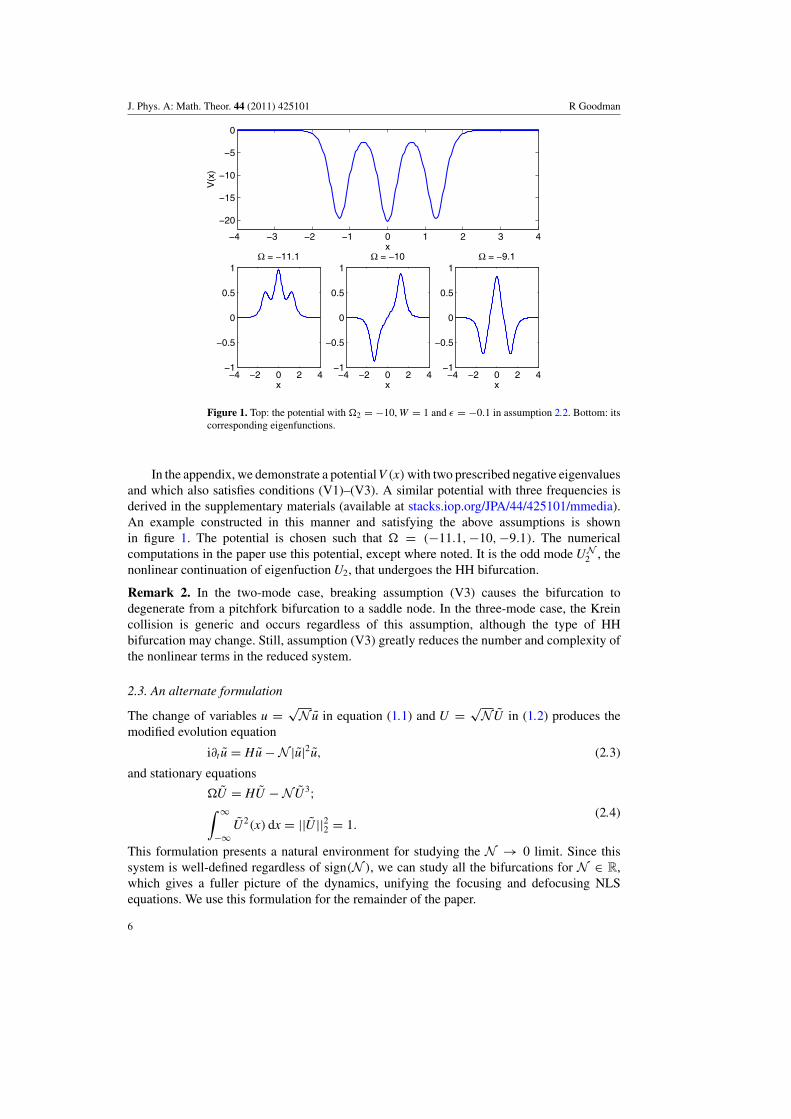
Figure 1. Top: the potential with �2 = −10, W = 1 and ε = −0.1 in assumption 2.2. Bottom: itscorresponding eigenfunctions.

In the appendix, we demonstrate a potentialV (x) with two prescribed negative eigenvaluesand which also satisfies conditions (V1)–(V3). A similar potential with three frequencies isderived in the supplementary materials (available at stacks.iop.org/JPA/44/425101/mmedia).An example constructed in this manner and satisfying the above assumptions is shownin figure 1. The potential is chosen such that � = (−11.1,−10,−9.1). The numericalcomputations in the paper use this potential, except where noted. It is the odd mode UN

2 , thenonlinear continuation of eigenfuction U2, that undergoes the HH bifurcation.

Remark 2. In the two-mode case, breaking assumption (V3) causes the bifurcation todegenerate from a pitchfork bifurcation to a saddle node. In the three-mode case, the Kreincollision is generic and occurs regardless of this assumption, although the type of HHbifurcation may change. Still, assumption (V3) greatly reduces the number and complexity ofthe nonlinear terms in the reduced system.

2.3. An alternate formulation

The change of variables u = √N u in equation (1.1) and U = √

NU in (1.2) produces themodified evolution equation

i∂t u = Hu − N |u|2u, (2.3)

and stationary equations

�U = HU − NU3;∫ ∞

−∞U2(x) dx = ||U ||22 = 1.

(2.4)

This formulation presents a natural environment for studying the N → 0 limit. Since thissystem is well-defined regardless of sign(N ), we can study all the bifurcations for N ∈ R,which gives a fuller picture of the dynamics, unifying the focusing and defocusing NLSequations. We use this formulation for the remainder of the paper.

6

J. Phys. A: Math. Theor. 44 (2011) 425101 R Goodman

Remark 3. This formulation has, in general, no bifurcation at N = 0: for almost all potentialsV (x), a smooth family of functions passes through any solution to system (2.4) at N = 0.

2.4. Hamiltonian systems, resonance and stability

The principal tool of this paper is to formally reduce system (2.3) to a finite-dimensional system.While the definitions given in this section refer to finite-dimensional systems, equivalentdefinitions exist for infinite-dimensional systems.

It is convenient to define the Hamiltonian in terms of n complex variables z =(z1, z2, . . . , zn) and their complex conjugates. In this setting, the Hamiltonian H is a realvalued function H(z, z) with canonical position vector given by q = z and momentum vectorby p = iz. The evolution equations are

id

dtz j = ∂

∂z∗j

H(z, z); j = 1, . . . , n. (2.5)

We often make reference to a ‘solution’ to a Hamiltonian H(z, z), by which we mean a solutionto the associated system (2.5).

2.4.1. Relative equilibria and relative periodic orbits. A solution to system (2.5) of the form

z = e−i�t z0,

i.e. a solution that is time-invariant in an appropriate rotating reference frame, is known asa relative equilibrium. Equation (2.4) describes such relative equilibria for NLS/GP (2.3).Similarly, a relative periodic orbit is a quasi-periodic orbit which appears periodic whenviewed in an appropriate rotating reference frame. A more technical definition of a relativeequilibrium (or periodic orbit) is a solution to (2.5) that corresponds to an equilibrium (orperiodic orbit) of a symmetry-reduced Hamiltonian derived from (2.5).

2.4.2. Quadratic Hamiltonian systems and resonances. A more standard formulation is tomake the change of variables q = (z + z)/

√2; p = (z − z/(i

√2)), which is canonical, i.e. it

preserves the Hamiltonian structure q j = ∂H/∂ p j and p j = −∂H/∂q j. Writing x = (qp

),the

equations of motion are ddt x = J∇H; J = ( 0 I

−I 0

).

Assuming that x = 0 is an equilibrium, then H = H2(x)+O(|x|3),where H2(x) = 〈x, Kx〉for some symmetric matrix K. The linear stability of the trivial solution is determined by theeigenvalues λ j of the matrix JK. The real and imaginary parts of the eigenvalues determine,respectively, the growth and decay rates of the solution, and the oscillation frequency of smallsolutions. The solution is unstable if any eigenvalues λ j satisfy �λ j > 0.

If the trivial solution is neutrally linearly stable, then JK has n complex conjugate pairsof eigenvalues λ = ±i� j on the imaginary axis, the natural frequencies of the system. If theseeigenvalues are distinct and nonzero, then the matrix JK is diagonalizable. Any solution to thelinear system is of the form

x =n∑

j=1

�(c j e−i� jtVj), (2.6)

where Vj is an eigenvector corresponding to i� j.Topologically, such a solution lies on an n-dimensional torus T

n in the 2n-dimensionalphase space. The analysis in this paper requires some understanding of resonances inHamiltonian systems, see e.g. Wiggins [28]. A resonance relation is a solution to the equation

〈k,�〉 = 0 with k ∈ Zn\{0}. (2.7)

7

J. Phys. A: Math. Theor. 44 (2011) 425101 R Goodman

The sum

|k| =n∑

j=1

|k j|

defines the order of a given resonance; e.g. a frequency vector � satisfying assumption 2.2with ε = 0, together with the vector k = (1,−2, 1), satisfies equation (2.7) and defines aresonance of order 4. The number of linearly independent vectors k that solve equation (2.7)is the multiplicity of the resonance. In the absence of such resonances, each solution (2.6)is dense on T

n. Given a resonance with multiplicity m, the solutions are confined to, anddense on, (n − m)-dimensional subsets of T

n which are themselves topologically equivalentto T

n−m. To understand this, think of the two-dimensional case. If there are two non-resonantfrequencies, any nonzero solution is dense on a two-torus, so its closure is two-dimensional,but if the two frequencies are rationally related, then each one-dimensional orbit is closed. Theclosed orbits lie on the level sets of an additional conservation law within T

2. A system witha near-resonance, 〈k,�〉 � 1 but non-zero, and small nonzero nonlinear terms will have anearly conserved quantity. Averaging methods then allow us to decrease the dimension of thesystem and obtain simpler equations that accurately approximate solutions for long but finitetimes.

While our procedure is to first derive a finite-dimensional Hamiltonian approximation toNLS and apply averaging methods to analyze this finite-dimensional system, Bambusi andcollaborators have applied such methods directly to a variety of PDE systems [29–31], themost relevant being [32]. We return to this theme in the conclusion, after more of the technicaldetails have been introduced.

2.4.3. Bifurcations. Bifurcation points, locations in parameter space where the stability,type, or number of solutions changes may be classified into different types, or normal forms.A normal form for a system of differential equations is any equivalent system of differentialequations, obtainable by a change of variables, in which the dynamics are particularly simpleto understand [28]. We talk more about normal forms for Hamiltonian systems in section 3.3.

In Hamiltonian systems, it is well-known (Williamson’s theorem) that if λ is an eigenvalue,then so are −λ, λ, and −λ. This implies that the eigenvalues can occur in four types ofgroupings, up to multiplicity: complex quadruplets (Krein quartets) {λ, λ,−λ,−λ} withnonzero real and imaginary parts, real-valued pairs {λ,−λ}, purely imaginary pairs {iμ,−iμ}and zero eigenvalues of even algebraic multiplicity.

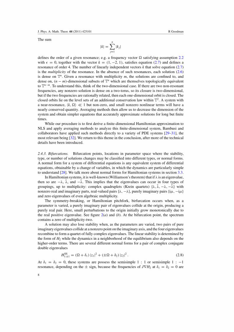
The symmetry-breaking, or Hamiltonian pitchfork, birfurcation occurs when, as aparameter is varied, a purely imaginary pair of eigenvalues collide at the origin, producing apurely real pair. Here, small perturbations to the origin initially grow monotonically due tothe real positive eigenvalue. See figure 2(a) and (b). At the bifurcation point, the spectrumcontains a zero of multiplicity-two.

A solution may also lose stability when, as the parameters are varied, two pairs of pureimaginary eigenvalues collide at a nonzero point on the imaginary axis, and the four eigenvaluesrecombine to form a quartet of fully complex eigenvalues. The linear stability is determined bythe form of H2 while the dynamics in a neighborhood of the equilibrium also depends on thehigher-order terms. There are several different normal forms for a pair of complex conjugatedouble eigenvalues

HSS1:±1 = (� + δ1) |z1|2 + (±� + δ2) |z2|2 . (2.8)

At δ1 = δ2 = 0, these systems are possess the semisimple 1 : 1 or semisimple 1 : −1resonance, depending on the ± sign, because the frequencies of J∇H2 at δ1 = δ2 = 0 are

8

J. Phys. A: Math. Theor. 44 (2011) 425101 R Goodman

(1)

(2) (3)

Re(λ)

Im(λ)(a)

(1)

(2)

(3)

Re(λ)

Im(λ)(c) (1) (2) (3)

Re(λ)Im(λ)

(d )

(1)

(2)

(3)

(b)

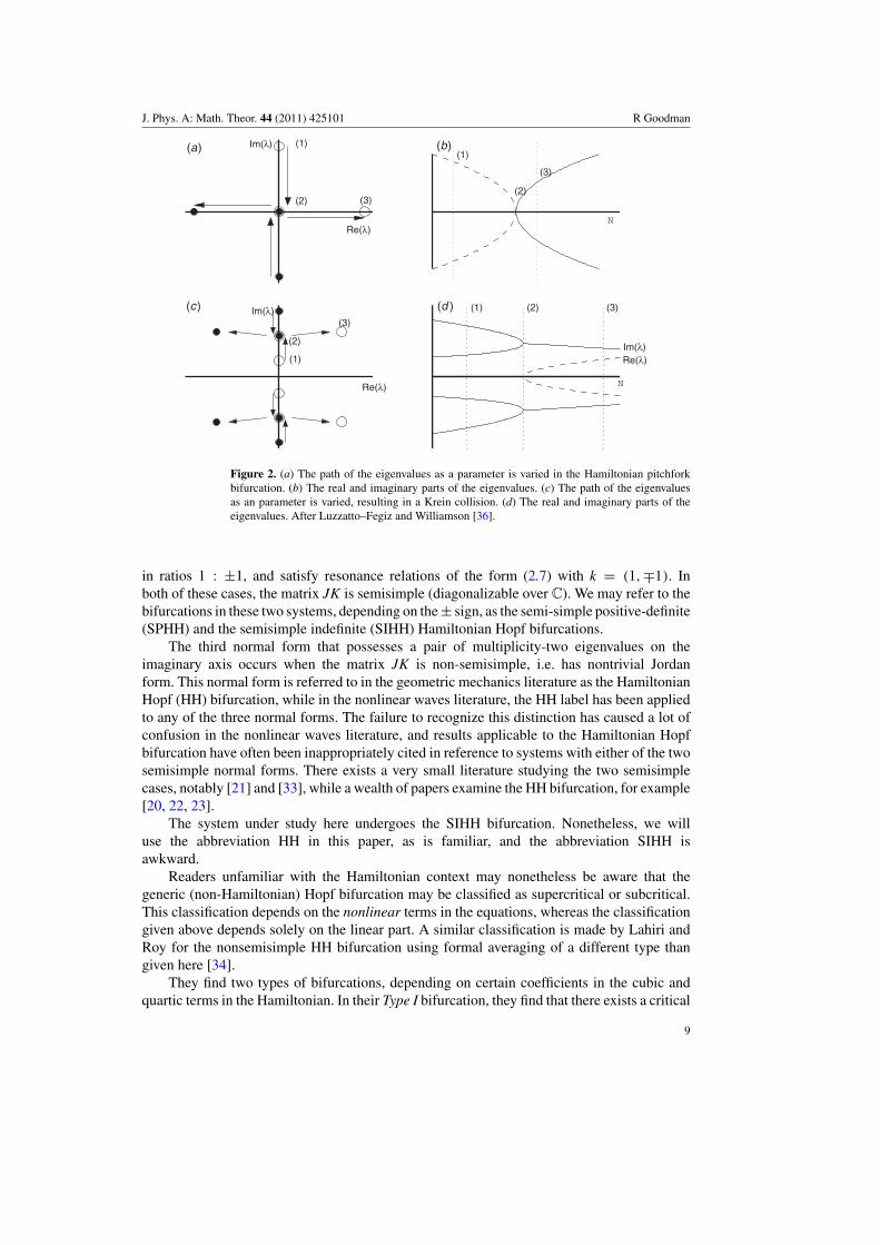
Figure 2. (a) The path of the eigenvalues as a parameter is varied in the Hamiltonian pitchforkbifurcation. (b) The real and imaginary parts of the eigenvalues. (c) The path of the eigenvaluesas an parameter is varied, resulting in a Krein collision. (d) The real and imaginary parts of theeigenvalues. After Luzzatto–Fegiz and Williamson [36].

in ratios 1 : ±1, and satisfy resonance relations of the form (2.7) with k = (1,∓1). Inboth of these cases, the matrix JK is semisimple (diagonalizable over C). We may refer to thebifurcations in these two systems, depending on the ± sign, as the semi-simple positive-definite(SPHH) and the semisimple indefinite (SIHH) Hamiltonian Hopf bifurcations.

The third normal form that possesses a pair of multiplicity-two eigenvalues on theimaginary axis occurs when the matrix JK is non-semisimple, i.e. has nontrivial Jordanform. This normal form is referred to in the geometric mechanics literature as the HamiltonianHopf (HH) bifurcation, while in the nonlinear waves literature, the HH label has been appliedto any of the three normal forms. The failure to recognize this distinction has caused a lot ofconfusion in the nonlinear waves literature, and results applicable to the Hamiltonian Hopfbifurcation have often been inappropriately cited in reference to systems with either of the twosemisimple normal forms. There exists a very small literature studying the two semisimplecases, notably [21] and [33], while a wealth of papers examine the HH bifurcation, for example[20, 22, 23].

The system under study here undergoes the SIHH bifurcation. Nonetheless, we willuse the abbreviation HH in this paper, as is familiar, and the abbreviation SIHH isawkward.

Readers unfamiliar with the Hamiltonian context may nonetheless be aware that thegeneric (non-Hamiltonian) Hopf bifurcation may be classified as supercritical or subcritical.This classification depends on the nonlinear terms in the equations, whereas the classificationgiven above depends solely on the linear part. A similar classification is made by Lahiri andRoy for the nonsemisimple HH bifurcation using formal averaging of a different type thangiven here [34].

They find two types of bifurcations, depending on certain coefficients in the cubic andquartic terms in the Hamiltonian. In their Type I bifurcation, they find that there exists a critical

9

J. Phys. A: Math. Theor. 44 (2011) 425101 R Goodman

nonlinearity coefficient Ncrit > 0. For N > Ncrit, the averaged equations possess a periodicorbit a distance d ∝ √

N > Ncrit from the origin, regardless of whether the nonlinear termsare subcritical or supercritical. In their Type II bifurcation, there exists no nonzero periodicorbit near zero on the unstable side of the bifurcation. Johansson makes a similar observationin his study of the NLS trimer [11] but does not comment on the difference between thesemisimple and non-semisimple bifurcations—in fact, a straightforward computation showsthe bifurcation for the trimer is semisimple, so the results of Lahiri and Roy do not apply.The analysis of Chow and Kim [33] serves a similar purpose for the SIHH bifurcation, but thedynamics are too varied to fit into a simple dichotomy.

2.4.4. Krein Signatures. Whether the collision of eigenvalues on the imaginary axis leadsto instability is determined by the Krein signatures [35] associated with them. Let Iω be theeigenspace corresponding to the eigenvalues ±iω, with basis {ξ1, . . . , ξ2n}. Defining K{ω} to bethe restriction of K to Iω, which can be constructed explicitly, using (complex) inner productsto define a matrix

K{ω}j,k = 〈ξ j, Kξk〉.

Since K{ω} is self-adjoint, we can define the positive (respectively, negative) Krein signature ofIω to be the number of positive (resp., negative) eigenvalues of K{ω}.1 An important theorem onstability [35] states that if Iω has mixed signature, i.e. if both its positive and negative signaturesare nonzero, then upon perturbation the eigenvalues may split into a Krein quartet, and thatthis cannot happen if Iω has purely positive (or purely negative) signature. As a consequence,when two pairs of purely imaginary eigenvalues of opposite Krein signature collide, theygenerically split into a Krein quartet, indicating that the origin has become unstable, withoscillatory dynamics due to their nonzero imaginary parts as sketched in figure 2(c) and (d).

3. The finite-dimensional model

3.1. Derivation of the model

We decompose the solution to equation (2.3) as the following time-dependent linearcombination:

u = c1(t)U1(x) + c2(t)U2(x) + c3(t)U3(x) + η(x; t), (3.1)

where the eigenfunctions Uj, defined in equation (2.1), are orthonormal and, for all t, η(x; t)is orthogonal to the discrete eigenspace, i.e.

〈Ui,Uj〉 = δi, j and 〈η(·, t),Uj〉 = 0, for i, j = 1, 2, 3.

We define the projection operators on to the discrete eigenmodes

� jζ = 〈Uj, ζ 〉Uj for j = 1, 2, 3, (3.2)

and onto the continuous spectrum

�Cζ = ζ − (�1 + �2 + �3)ζ .

1 Mackay [35] provides a complete definition, which is also well defined for the cases of real eigenvalues and complexquartets as well as purely imaginary eigenvalues.

10

J. Phys. A: Math. Theor. 44 (2011) 425101 R Goodman

Substituting the decomposition (3.1) into NLS/GP (2.3) and applying these four projectionoperators gives evolution equations for the components of the decomposition. The followingsystem of equations is equivalent to (2.3) under the assumptions of section 2.2:

idc1

dt− �1c1 + N

[a1111|c1|2c1 + a1113

(c2

1c3 + 2|c1|2c3) + a1122

(2c1|c2|2 + c1c2

2

)+ a1133

(2c1|c3|2 + c1c2

3

) + a1223(c2

2c3 + 2|c2|2c3)

+ a1333|c3|2c3] = R1(c1, c2, c3, η);

idc2

dt− �2c2 + N

[a1122

(c2

1c2 + 2|c1|2c2) + 2a1223(c1c2c3 + c1c2c3 + c1c2c3)

+ a2222|c2|2c2 + a2233(2c2|c3|2 + c2c2

3

)] = R2(c1, c2, c3, η);idc3

dt− �3c3 + N

[a1113|c1|2c1 + a1133

(c2

1c3 + 2|c1|2c3) + a1223

(2c1|c2|2 + c1c2

2

)+ a1333

(2c1|c3|2 + c1c2

3

) + a2233(c2

2c3 + 2|c2|2c3)

+ a3333|c3|2c3] = R3(c1, c2, c3, η);

i∂tη − Hη + N |η|2η = RC(c1, c2, c3, η), (3.3)

wherea jklm = 〈u j, ukulum〉

and we have used the invariance of the coefficients ajklm under permutation of the four indicesand the fact that a jklm = 0 if ( j + k + l +m) is odd. The parameters are calculated numericallyas needed for the numerical simulations. The remainder terms Rj are the projections of theremaining nonlinear terms of (2.3) onto the discrete eigenfunctions:

Rj = −N · � jF,

where � j is given in equation (3.2) and

F = |c1U1 + c2U2 + c3U3 + η|2(c1U1 + c2U2 + c3U3 + η)

− |c1U1 + c2U2 + c3U3|2(c1U1 + c2U2 + c3U3).

The remainder term in the continuum portion is

RC = −N · �CG,

whereG = |c1U1 + c2U2 + c3U3 + η|2 (c1U1 + c2U2 + c3U3 + η) − |η|2 η.

Ignoring the contributions of η(x; t) to the solution yields a finite-dimensionalapproximation to (3.3); the reasoning for the change of notation N → N is describedafterward:

idc1

dt− �1c1 + N

[a1111|c1|2c1 + a1113

(c2

1c3 + 2|c1|2c3) + a1122

(2c1|c2|2 + c1c2

2

)+ a1133

(2c1|c3|2 + c1c2

3

) + a1223(c2

2c3 + 2|c2|2c3) + a1333|c3|2c3

] = 0

idc2

dt− �2c2 + N

[a1122

(c2

1c2 + 2|c1|2c2) + 2a1223(c1c2c3 + c1c2c3 + c1c2c3)

+ a2222|c2|2c2 + a2233(2c2|c3|2 + c2c2

3

)] = 0

idc3

dt− �3c3 + N

[a1113|c1|2c1 + a1133

(c2

1c3 + 2|c1|2c3) + a1223

(2c1|c2|2 + c1c2

2

)+ a1333

(2c1|c3|2 + c1c2

3

) + a2233(c2

2c3 + 2|c2|2c3) + a3333|c3|2c3

] = 0. (3.4)

11

J. Phys. A: Math. Theor. 44 (2011) 425101 R Goodman

We have introduced the following slight change of notation in this equation. As system (3.3)is equivalent to equation (2.3), it conserves the L2 norm

|c1|2 + |c2|2 + |c3|2 + ‖η‖22 = 1.

This implies that |c1|2 + |c2|2 + |c3|2 � 1, while system (3.4) possesses a finite-dimensionalconserved quantity corresponding to the photon number of system (1.1),

|c1|2 + |c2|2 + |c3|2 = 1. (3.5)

The conserved quantities in systems (2.3) and (3.4) are not equivalent, since the contributionof η(x, t) is ignored in the latter. Recall that N represents the total intensity and the sign ofthe nonlinearity in equation (1.1). Since the meaning of N is slightly changed from equation(2.3) to system (3.4), we introduce the new constant N.

The above reduction demands some justification, either numerical or rigorous. One checkis whether a numerically computed solution to (1.1) whose initial condition consists of a linearsuperposition of the eigenmodes stays close to the manifold η(x, t) = 0 for long times. OurPDE simulations, which are described in section 5.2 were run over long times, up to 20 000oscillations of the phase θ (t). Although they were run with absorbing boundary conditions,the computed L2 norm of the solution was in all cases conserved to within half of a percent,and the L2 norm of the projection onto the three eigenfunctions conserved to within 0.6percent. Further, figure 6 shows good qualitative agreement, and for shorter times quantitativeagreement, between solutions to (1.1) and the approximation (3.4).

To rigorously justify the above assumptions is, of course, a significant task, and one whichwe delay to a subsequent paper. It should proceed in largely the same way as recent results.Here we discuss those results and in what sense those results justify the finite-dimensionaltruncation. Kirr et al [4] prove using a Lyapunov–Schmidt argument that standing wavesgiven as the continuations of the linear eigenfunctions are well-approximated by solutionsto the finite dimensional system, and that the critical amplitude at which such solutions losestability in symmetry-breaking bifurcations is asymptotically close to the bifurcation valuefor the finite-dimensional problem. Marzuola and Weinstein [6] prove a shadowing theorem,in which certain quasiperiodic solutions to the finite-dimensional system are shadowed bysolutions to NLS/GP (1.1) over long but finite times using an infinite-dimensional Floquetargument. This approach required the use of Strichartz estimates, and we should be able toprove similar theorems regarding periodic and quasiperiodic solutions in the present case.Pelinovsky and Phan [7] use a normal form argument that proves the results of Kirr withoutLyapunov–Schmidt, and obtains short-time shadowing theorems like Marzuola for arbitrarysmall initial conditions, not just certain periodic orbits, without the need for Floquet analysisand using much simpler inequalities, at the cost of the estimates being valid on significantlyshorter timescales. Of course, since the numerics below suggest that both the PDE and ODEevolve chaotically, such a shadowing theorem may have to be replaced by a much weakerstatement. The proofs given in the above references depend on stricter assumption than thosegiven in (S1)–(V3), particularly inequalities involving the coefficients ai jkl .

3.2. Model reduction via symmetry

To understand the dynamics of system (3.4), it is useful to use the invariance of H underc j → eiαc j to reduce the number of degrees of freedom from three to two. This reduction isbased on the Hamiltonian form

12

J. Phys. A: Math. Theor. 44 (2011) 425101 R Goodman

H = �1|c1|2 + �2|c2|2 + �3|c3|2 − N[

12 a1111|c1|4 + a1113|c1|2(c1c3 + c1c3)

+ a1122(

12 c2

1c22 + 2|c1|2|c2|2 + 1

2 c21c2

2

) + a1133(

12 c2

1c23 + 2|c1|2|c3|2 + 1

2 c21c2

3

)+ a1223

(2|c2|2(c1c3 + c1c3) + c1c2

2c3 + c1c22c3

) + a1333|c3|2(c1c3 + c1c3)

+ 12 a2222|c2|4 + a2233

(12 c2

2c23 + 2|c2|2|c3|2 + 1

2 c22c2

3

) + 12 a3333|c3|4

](3.6)

with evolution equations

ic j = ∂H

∂ c j; j = 1, 2, 3. (3.7)

We simplify the equations using generalized action-angle coordinates

c1(t) = σ1(t) eiθ (t); c2(t) = ρ(t) eiθ (t); c3(t) = σ3(t) eiθ (t), (3.8)

where ρ(t), θ (t) ∈ R. ODEs for these variables are determined by inserting (3.8) into equations(3.6) and (3.7). The c2 equation determines the evolution of θ (t) in terms of σ1 and σ3

θ (t) = −�2 + N[a2222(1 − |σ1|2 − |σ3|2) + 1

2 a1122(σ 2

1 + 4|σ1|2 + σ 21

)+ a1223(2σ3σ1 + 2σ1σ3 + σ1σ3 + σ1σ3) + 1

2 a2233(σ 2

3 + 4|σ3|2 + σ 23

)]. (3.9)

This equation and the conservation law (3.5) are used to eliminate θ and ρ from the evolutionequations for σ1(t) and σ3(t). These are integrated to give a reduced Hamiltonian dependingsolely on N, σ1, σ3, and their complex conjugates:

HR = (−W + ε)|σ1|2 + (W + ε) |σ3|2 − N[

12 a1111 |σ1|4 + a1113 |σ1|2 (σ1σ3 + σ1σ3)

+ 12 a1122(1 − |σ1|2 − |σ3|2)

(σ 2

1 + 4|σ1|2 + σ 21

)+ a1133

(12σ 2

1 σ 23 + 2|σ1|2|σ3|2 + 1

2 σ 21 σ 2

3

)+ a1223(1 − |σ1|2 − |σ3|2)(σ1σ3 + 2σ1σ3 + 2σ1σ3 + σ1σ3)

+ a1333|σ3|2(σ1σ3 + σ1σ3)

+ 12 a2222(1 − |σ1|2 − |σ3|2)2 + 1

2 a2233(1 − |σ1|2 − |σ3|2)(σ 2

3 + 4|σ3|2 + σ 23

)+ 1

2 a3333|σ3|4]. (3.10)

The term c2(t) may be recovered using the conservation law (3.5) to obtain ρ(t) andequation (3.9) for θ (t).

Remark 4. This reduction involves defining a reference phase θ (t) and thus leads to reducedequations that are not equivariant with respect to rotation by a phase.

3.3. Averaging and further reduction of the ODE

We further reduce the system using averaging methods. This puts the equations into normalform, which identifies which terms in HR have a significant effect on the dynamics at leadingorder. We formally apply the von Zeipel procedure, which applies when there is a resonancebetween eigenvalues [28, 37]. The averaged equations preserve some but not all features ofthe full system of equations—for example, hyperbolic equilibria and their local un/stablemanifolds are preserved, but homoclinic orbits are not. The averaged system Haverage, equation(3.19), is completely integrable, but we do not expect general Hamiltonians, such as (3.10), tobe. Our numerical computations, typified by figure 6, suggest that the full system is chaoticand thus not integrable.

To put the system in the correct form for averaging, we make two exact changes ofvariables. After using definition (4.4), and replacing ε in equation (2.2) by

ε → sε

13

J. Phys. A: Math. Theor. 44 (2011) 425101 R Goodman

with ε � 0 and s = ±1, we first make the change of variables to canonical polar coordinates

σ j → √ρ je

iθ j ; j = 1, 3,

yielding a Hamiltonian:

Hpolar = Wρ1 − Wρ3 − εs(ρ1 + ρ3) + εν[(a1122 cos 2θ1 + 2a1122 − a2222)ρ1

+ 2a1223(2 cos (θ1 − θ3) + cos (θ1 + θ3))√

ρ1√

ρ3

+ (a2233 cos 2θ3 − a2222 + 2a2233)ρ3

+ 12 (−2a1122 cos 2θ1 + a1111 − 4a1122 + a2222)ρ

21

+ 2((a1113 − 2a1223) cos (θ1 − θ3) − a1223 cos (θ1 + θ3))ρ3/21 ρ

1/23

− (a1122 cos 2θ1 − a1133 cos 2(θ1 − θ3) + a2233 cos 2θ3

+ 2a1122 − 2a1133 − a2222 + 2a2233)ρ1ρ3

− 2((2a1223 − a1333) cos (θ1 − θ3) + a1223 cos (θ1 + θ3))ρ1/21 ρ

3/23

+ 12 (−2a2233 cos 2θ3 + a2222 − 4a2233 + a3333)ρ

23

]. (3.11)

Averaging methods allow one to simplify a system by replacing some or all of its oscillatoryterms by their means, which is accomplished using a sequence of near-identity changes ofvariables. Leading-order linear terms that satisfy a resonance condition, as in (2.7), rendersome of these equations unsolvable due to zero denominators. Were it not for such resonancesbetween the eigenvalues, one could formally remove all terms containing trigonometricfunctions and fractional powers of ρ1 and ρ3, putting the system in the so-called Birkhoffnormal form. In the present case, the leading order linear part H2 = Wρ1 − Wρ3 is 1 : −1resonant (semisimple and indefinite), so the system cannot be completely averaged and theGustavson normal form applies, in which all but the resonant terms are averaged away. Formore information see Wiggins [28, section 19.10, section 20.9].

The canonical change of variables

θ1 = φ1, θ3 = −φ1 + φ3, ρ1 = I1 + I3, ρ3 = I3

puts the Hamiltonian into the form

Hreduced(�I, �φ) = H0(I1) + εH1(I1, I3, φ1, φ3), (3.12)

whereH0(I1) = WI1 and H1 = Hmean

1 (I1, I3) + Hosc1 (I1, I3, φ1, φ3)

and Hosc1 has period π in φ1 and 2π in φ3. In general, the term H0 may be written as the inner

productH0 = 〈ω,�I〉,

so that, in this case, ω = (W, 0). Equation (3.12) shows that φ1 oscillates on an O(1) timescale since d

dt φ1 = W + O(ε), while I1, I3 and φ3 oscillate slowly, on an O(ε−1) time scale.For this reason φ1, but not φ3, can be averaged out.

In the present problem, Hosc1 contains five terms, details omitted:

Hosc1 =

∑k∈K

Hk1 (I1, I3) cos 〈k, �φ〉;

K = Kres ∪ Knon = {(0, 1)} ∪ {(2, 0), (2,−1), (2,−2), (4,−2)}.Applying definition (2.7) the ordered pair (0, 1) ∈ Kres is resonant with ω, while the four inKnon are not.

14

J. Phys. A: Math. Theor. 44 (2011) 425101 R Goodman

The von Zeipel averaging procedure yields a partially averaged Hamiltonian as a formalpower series in ε,

I j = ∂S

∂φ j, ψ j = ∂S

∂Jj, (3.13)

S(J, φ, ε) = 〈�J, �φ〉 + εS1(�J, �φ) + · · · (3.14)

H(�J, �ψ) = H0(I) + εH1(�J, �ψ) + · · · . (3.15)

Equations of the form (3.13) generate a canonical near-identity change of variables (I, φ) →(J, ψ) for any generating function S(J, φ), the downside being that S must be inverted in orderto find J. A more modern approach using Lie transforms does not have this problem. Pluggingthe expansion for I = Sφ into the Hamiltonian (3.12), setting this equal to the series (3.15) forH and equating orders of ε, one finds at O(1), H0 = H0, and at order ε,

H1(J, ψ) = 〈∇�JH0,∇�φS1〉 + H1(�J, �ψ) = 〈ω,∇�φS1〉 + H1(�J, �ψ).

The terms in S1 are chosen to eliminate the fast phases from H1. The method proceedsby eliminating terms in H1 of the form Hk

1 cos 〈k, �φ〉 one at a time by solving homologicalequations of the form

(ω · ∇�φ )Sk1 + Hk

1 cos 〈k, �φ〉 = 0.

For k ∈ Kres, this equation is unsolvable, since cos 〈k, �φ〉 is in the nullspace of the operatorω · ∇φ . Terms involving k ∈ Knon may be eliminated, so that

S1 =∑

k∈Knon

−Hk1

〈k, ω〉 sin 〈k, �φ〉.

This transforms the Hamiltonian to

H(�J, �ψ) = WJ1 + εH1(J1, J3, ψ3) + ε2Hremainder(J1, J3, ψ1, ψ3; ε), (3.16)

where

H1(J1, J3, ψ3) = α1J1 + α3J3 + α1,1J21 + α1,3J1J3 + α3,3J2

3

+ 21223ν(J1 + 2J3 − 1)√

J3

√J3 + J1 cos ψ3 (3.17)

and Hremainder is 2π -periodic in ψ1. We delay writing down the coefficients.System (3.16) is in the proper form for the reduction procedure of [38, section 4.8]. We

consider the dynamics on the level set H = hW and solve for J1 in (3.17) as a series in ε.Such a solution exists when ∂

∂J1H �= 0, or equivalently when d

dt ψ1 �= 0. In this case ψ1 is atime-like variable; the reduction then gives simplified equations for the evolution of (J3, ψ3)

with respect to ψ1. The ansatz

J1 = L(J3, ψ3; h) = J(0)

1 + εJ(1)

1 + · · ·yields expansion

J(0)

1 = h; J(1)

1 = − 1

WH1(h, J3, ψ3)

and J3 and ψ3 evolve under the effective Hamiltonian

Hreduced(J3, ψ3, τ ; h) = −L = −h + ε

WH1(J3, ψ3; h) + ε2H2(J3, ψ3, τ ; h). (3.18)

15

J. Phys. A: Math. Theor. 44 (2011) 425101 R Goodman

Ignoring any terms independent of J3 and ψ3 that do not effect the dynamics

H1(J3, ψ3; h) = γ1J3 + γ2J23 + γ3

√J3

√J3 + h (2J3 + h − 1) cos ψ3

with

γ1 = 2s + (−a1111h + 2a1122(3h − 1) − 2a1133h − 2a2222(h − 1) + 2a2233(h − 1)) ν

γ2 = ν

2(−a1111 + 8a1122 − 4a1133 − 4a2222 + 8a2233 − a3333)

γ3 = 2νa1223.

Remark 5. The implicit function theorem will fail if there exists t0 such that dψ1

dt |t=t0 = ∂H∂J1

= 0;if ψ1 does not grow monotonically, it cannot be used as a proxy for time. Our simulationsshow this is the case, for example, in figure 6, row (d).

System (3.18) satisfies some easily verified smoothness requirements in order to apply theaveraging theorem, as stated by Guckenheimer and Holmes [38, theorem 4.1.1]. The theoremguarantees that there exists a change of variables

J = J3 + O(ε), ψ = ψ3 + O(ε)

such that the solution to the averaged system with Hamiltonian

Haverage = ε

WH1(J, ψ; h) (3.19)

agrees with solutions to system (3.18) with O(ε) error O(ε−1) timescales. Further, forsufficiently small ε, hyperbolic equilibria and their local invariant manifolds of system (3.19)correspond to hyperbolic periodic orbits and their local invariant manifolds of system (3.18).Similarly elliptic equilibria of (3.19) correspond to elliptic periodic solutions of (3.18).

By the conservation law (3.5), ρ1 and ρ3 in system (3.11) are confined to the triangle

0 � ρ1 � 1; 0 � ρ3 � 1; 0 � ρ1 + ρ3 � 1.

In system (3.18), this becomes a constraint on the conserved parameter h and the variable J,

−1 � h � 1; max (−h, 0) � J � 1 − h

2

in the case 0 � h � 1. In this case, the phase space is the disk J � 1−h2 .

Due to the higher-order terms H2 in equation (3.18), the conservation of h is onlyapproximate in system (3.18). Formally, one may perform a countable sequence of changes ofvariables that transform system (3.18) into completely integrable form. This corresponds todefining a change of variables as a power series in ε. Generally, this power series has radiusof convergence zero, because the full system is not itself integrable, which we can see fromthe apparent chaotic dynamics in the numerical solution given in figure 6(c). This suggeststhat the solution 6(b) is also very weakly chaotic, but with a much smaller chaotic region anda longer chaotic timescale.

4. Stability and dynamics near the first excited state: analysis

Just as other studies have begun by focusing on the destabilization of the ground state of thetwo-well system via symmetry breaking [4, 6, 7], the goal of this paper is to understand the

16

J. Phys. A: Math. Theor. 44 (2011) 425101 R Goodman

dynamics in the neighborhood of an HH bifurcation. We therefore consider the stability of,and the dynamics near, the antisymmetric mode U2(x, N), the nonlinear continuation of thefirst excited state U2 of equation (2.1). In the reduced system (3.10) this is just the dynamics inthe neighborhood of the origin. Future work will include a more thorough description of theglobal phase space including all the relative equilibria and relative periodic orbits for small N.

4.1. Relative equilibria of the reduced hamiltonian

We first look for relative equilibria of system (3.10) of the form(σ1(t)σ3(t)

)=

(xy

)e−i�t,

which correspond, ultimately, to standing wave solutions of equation (1.2). This calculationis well-covered by Kapitula et al [8] who demonstrate the existence of two types. The firstfamilies persist in the N → 0 limit. These correspond to the nonlinear deformations of theeigenfunctions defined in equation (2.1). The other family of solutions arise due to saddle-nodebifurcations. These bifurcations are shown to take place for N � ε, whereas we demonstrateHH bifurcations for N = O(ε). It is simple to show [4, 8] that a solution to equation (1.2)with real potential V (x) are up to a constant phase factor, a real-valued function, as are relativeequilibria of system (3.10). Thus, without loss of generality, we look for stationary solutionsof the form

(� − �1 + �2 + 3a1122N)x + 3a1223Ny + N((a1111 − 3a1122)x3 + 3(a1113 − a1223)x

2y

+ 3(a1133 − a1122)xy2 − (3a1223 − a1333)y3) = 0

3a1223Nx + (� + �2 − �3 + 3a2233N)y + N((a1113 − 3a1223)x3 + 3(a1133 − a2233)x

2y

+ 3(a1333 − a1223)xy2 − (3a2233 − a3333)y3) = 0

with x2 + y2 � 1 and x, y ∈ R.The simplest solution is

x = y = 0, � = �2 − a2222 (4.1)

which corresponds to an antisymmetric standing wave solution to (1.2), the nonlineardeformation of the eigenpair (U2,�2) of equation (2.1). There are two other standing-wavesolutions for small N. These satisfy x2 + y2 = 1, so we write x = cos θ (N), y = sin θ (N).Taylor expanding θ (N) and �(N) for small N yields two solutions, one with θ near zero,corresponding to the nonlinear deformation of the eigenfunction U1, and one with θ near π/2,corresponding to the continuation of the eigenfunction U3. For a complete enumeration of therelative equilibria of (1.2), see [8].

4.2. Linearization of PDE solutions

Letting (U,�) be a solution of system (2.4) and consider small time-dependent perturbationsof the form

u(x, t) = (U (x) + r(x, t) + is(x, t)

)e−i�t .

Then, linearizing and letting(r, s) = (R(x), S(x))eλt

yields the eigenvalue problem

λ

(R

S

)=

(0 −(� + ∂2

x − V (x) + NU2(x))

� + ∂2x − V (x) + 3NU2(x)

)(R

S

). (4.2)

17

J. Phys. A: Math. Theor. 44 (2011) 425101 R Goodman

While future studies will concentrate on analysis of this system in its own right, here we areinterested in comparing the results of numerical stability studies of this system with thosefound for the model ODE.

4.3. Linearization of ODE

First, we determine the linear stability of the solution (4.1), the trivial solution to system (3.10).By inserting the form (

σ1(t)σ3(t)

)=

(r1(t) + is1(t)r3(t) + is3(t)

)

into system (3.10), the linearized equations become

d

dt

⎛⎜⎜⎝

r1

r3

s1

s3

⎞⎟⎟⎠ =

(02 −M−

M+ 02

)⎛⎜⎜⎝

r1

r3

s1

s3

⎞⎟⎟⎠ ≡ M(ε, N)u, (4.3)

where 02 is a 2 × 2 matrix of zeros,

M± =(

W − ε + (m±a1122 − a2222)N m±a1223Nm±a1223N −W − ε + (a2233 + m±a2222)N

),

and m± = 2 ± 1. The matrix M(ε, 0) has imaginary eigenvalues λ±1,2 = ±i(�1 − �2) =

±i(−W + ε) and λ±3,2 = ±i(�3 − �2) = ±i(W + ε). For all N, M(ε) is symplectic, i.e.

M = JK where K is symmetric and

J =(

02 −II 02

)so that K =

(M+ 02

02 M−

).

4.4. Analytical criterion for ODE bifurcation

In this section, we compute an analytic condition for a Krein collision in system (3.10). TheKrein signatures associated with the frequencies ±(�2 −�1) and ±(�2 −�3) in system (4.3)are K(±i(�1 − �2)) = sign(�1 − �2) and K(±i(�3 − �2)) = sign(�3 − �2), implyingby assumption (S1), that their Krein signatures are opposite. Thus, their collision leads toinstability. In fact, the Krein signature can be interpreted as the direction of phase rotation, andsince �2 lies between �1 and �3, the Krein signatures can be determined without performingthis calculation.

Krein collisions occurs at N for which P(λ; N), the characteristic polynomial of M(ε, N),has multiple roots. As is generic for Hamiltonian systems, P contains only even powers of λ.Letting q = λ2 defines a quadratic polynomial p(q; N), which has a multiple root at N whereits discriminant vanishes. Defining

ν = N/ε, (4.4)

the discriminant is

�(ν) = ε2(d4(ε)ν4 + d3(ε)ν3 + d2(ε)ν2 + d1(ε)ν + d0(ε)) = 0, (4.5)

18

J. Phys. A: Math. Theor. 44 (2011) 425101 R Goodman

where

d4 = (3a1122 − 4a2222 + 3a2233)2(a2

1122 − 2a2233a1122 + 4a21223 + a2

2233

)ε2

d3 = 8(a1122 − a2233)(a1122 − a2222 + a2233)(3a1122 − 4a2222 + 3a2233)Wε

− 8(3a1122 − 4a2222 + 3a2233)(a21122 − 2a2233a1122 + 4a2

1223 + a22233)ε

2

d2 = 16(a1122 − a1223 − a2222 + a2233)(a1122 + a1223 − a2222 + a2233)W2

− 8(a1122 − a2233)(7a1122 − 8a2222 + 7a2233)Wε

+ 16(a2

1122 − 2a2233a1122 + 4a21223 + a2

2233

)ε2

d1 = 32(a1122 − a2233)Wε − 32(a1122 − a2222 + a2233)W2

d0 = 16W 2.

This is solved numerically or by a perturbation expansion ν = ν0 + O(ε) which gives doubleeigenvalues at

NKC,± = ε

−a1122 ± a1223 + a2222 − a2233+ O(ε2). (4.6)

Thus, there are Krein collisions for small values of ε, under the assumption that the denominatorof this equation is bounded away from zero.

4.5. Dynamics of the averaged system H1

We are interested in the dynamics near the trivial solution of system (3.10), (σ1, σ3) = (0, 0),which we showed in the previous section to destabilize via a semisimple implicit HHbifurcation.

This fixed point lies on the level set h = 0 in the truncated averaged system (3.19), so wecan gain insight into the behavior of solutions to the system near this solution by looking at itsphase space for h = 0. There is a slightly different structure for general h, which is the subjectof ongoing investigation.

First, we define two invariant subspaces: �odd is simply the origin in system (3.10),corresponding to all the energy in system (2.3) being in the mode U2(x). In the reduced system(3.19), this invariant set only intersects the set h = 0 where it corresponds to the left boundaryJ = 0. The second subspace is

�even = {(σ1, σ3)||σ1|2 + |σ3|2 = 1}

corresponding to the case where all the energy in system (2.3) is in the two modes with evensymmetry. In the averaged system (3.19), �even is simply the right boundary J = 1−h

2 .

On the set h = 0, the level set of system (3.19) corresponding to the origin in (z1, z3, z1, z3)-space is

S0 = {(J, ψ)|γ1J + γ2J2 + γ3(2J2 − J) cos ψ = 0}= �odd ∪

{(J, ψ)

∣∣∣∣cos ψ = γ1 + γ2J

γ3(1 − 2J)

}.

There exist fixed points on �odd if the second set contains points with J = 0. At these points,

cos ψ = γ1

γ3= − (a1122 − a2222 + a2233) ν − s

a1223ν. (4.7)

These solutions exist if |γ1/γ3| � 1 and there exist bifurcations when the right-hand side is±1, i.e. at

νKC = s

±a1223 + a1122 − a2222 + a2233,

19

J. Phys. A: Math. Theor. 44 (2011) 425101 R Goodman

0 0.1 0.2 0.3 0.4 0.5−3

−2

−1

0

1

2

3

J

ψ

(a) N=0.25

0 0.1 0.2 0.3 0.4 0.5−3

−2

−1

0

1

2

3

J

ψ

(b) N=0.5

0 0.1 0.2 0.3 0.4 0.5−3

−2

−1

0

1

2

3

J

ψ

(c) N=1

0 0.1 0.2 0.3 0.4 0.5−3

−2

−1

0

1

2

3

J

ψ

(d ) N=1.5

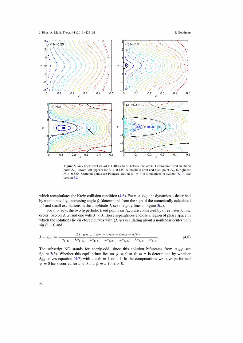
Figure 3. Gray lines: level sets of H1. Black lines: heteroclinic orbits. Heteroclinic orbit and fixedpoint JNO toward left appears for N > 0.445; heteroclinic orbit and fixed point JNE to right forN > 0.530. Scattered points are Poincare section ψ1 = 0 of simulations of system (3.10); seesection 5.2.

which recapitulates the Krein collision condition (4.6). For ν < νKC, the dynamics is describedby monotonically decreasing angle ψ (determined from the sign of the numerically calculatedγ1) and small oscillations in the amplitude J; see the gray lines in figure 3(a).

For ν > νKC, the two hyperbolic fixed points on �odd are connected by three heteroclinicorbits: two on �odd and one with J > 0. These separatrices enclose a region of phase space inwhich the solutions lie on closed curves with (J, ψ) oscillating about a nonlinear center withsin ψ = 0 and

J = JNO ≡ 2 (a1122 ± a1223 − a2222 + a2233 − s/ν)

−a1111 − 8a1122 − 4a1133 ± 4a1223 + 4a2222 − 8a2233 + a3333. (4.8)

The subscript NO stands for nearly-odd, since this solution bifurcates from �odd; seefigure 3(b). Whether this equilibrium lies on ψ = 0 or ψ = π is determined by whetherJNO solves equation (4.7) with cos ψ = 1 or −1. In the computations we have performedψ = 0 has occurred for s < 0 and ψ = π for s > 0.

20

J. Phys. A: Math. Theor. 44 (2011) 425101 R Goodman

4.5. Additional structure from the averaged system. A similar bifurcation exists involving�even. Two hyperbolic equilibria on �even exist at

J = 1

2; cos ψF = −γ1 − γ2

γ3. (4.9)

These exist only if the right hand side has magnitude less than one which gives a necessarycondition on the amplitude ν � νF for their existence, where

νF = s

14 a1111 − a1122 + a1133 ∓ a1223 − a2233 + 1

4 a3333. (4.10)

The dynamics of the averaged system near this structure are exactly analogous to thedynamics near �odd described above. For ν > νF, equation (4.9), the two saddles are connectedby three heteroclinic orbits, two of them contained in �even and a third one surrounding anadditional elliptic equilibrium with J = JNE (nearly even) and ψ = π or ψ = 0; seefigure 3(c).

Remark 6. For h �= 0, the structure near �even persists: there is a critical amplitude νF(h)

which approaches νF as h → 0, and for ν > νF(h), there exist three fixed points and threeheteroclinic orbits. Near �odd, the behavior is somewhat different as will be explained furtherin an upcoming article. These differences do not effect the claims made here.

Note that the equilibria of system (3.19) found in this section correspond to periodicorbits of equation (3.10) and are not solutions to system (2.4). The averaged system (3.19) isvalid for small values of ε and describes the dynamics for small |N| demonstrated numericallyin figure 5. More concretely, the averaged system possesses the bifurcations described byequation (4.6), but not the other two roots of equation (4.5) that may exist for N = O(1).

The evolution in the averaged system shown in figure 3 appears very similar to that in[6, figure 8] for a two-well defect. The separatrix that bifurcates from �odd is a close analog ofthe homoclinic origin to the origin in the Hamiltonian pitchfork bifurcation. The equilibria andseparatrix that bifurcate from �even have no analog in their model. The behavior of solutions to(3.10) closely follows that of the averaged system for small ν but demonstrates torus break-upand chaos for larger values of ν, as discussed in section 5.2. This is qualitatively different fromMarzuola and Weinstein, because the system they study is integrable.

5. Stability and dynamics near the first excited state: numerical simulations

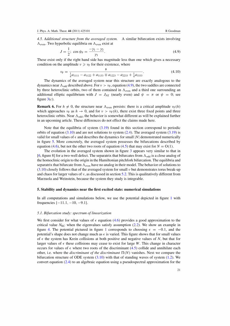
In all computations and simulations below, we use the potential depicted in figure 1 withfrequencies {−11.1,−10,−9.1}.

5.1. Bifurcation study: spectrum of linearization

We first consider for what values of ε equation (4.6) provides a good approximation to thecritical value NKC when the eigenvalues satisfy assumption (2.2). We show an example infigure 4. The potential pictured in figure 1 corresponds to choosing ε = −0.1, and thepotential’s shape does not change much as ε is varied. This figure shows that for small valuesof ε the system has Krein collisions at both positive and negative values of N, but that forlarger values of ε these collisions may cease to exist for large W . This change in characteroccurs for values of ε where two roots of the discriminant (4.5) collide and annihilate eachother, i.e. where the discriminant of the discriminant �(N) vanishes. Next we compare thebifurcation structure of ODE system (3.10) with that of standing waves of system (1.2). Weconvert equation (2.4) to an algebraic equation using a pseudospectral approximation for the

21

J. Phys. A: Math. Theor. 44 (2011) 425101 R Goodman

−0.8 −0.6 −0.4 −0.2 0 0.2 0.4 0.6 0.8

−8

−6

−4

−2

0

2

4

6

ε

NK

C±

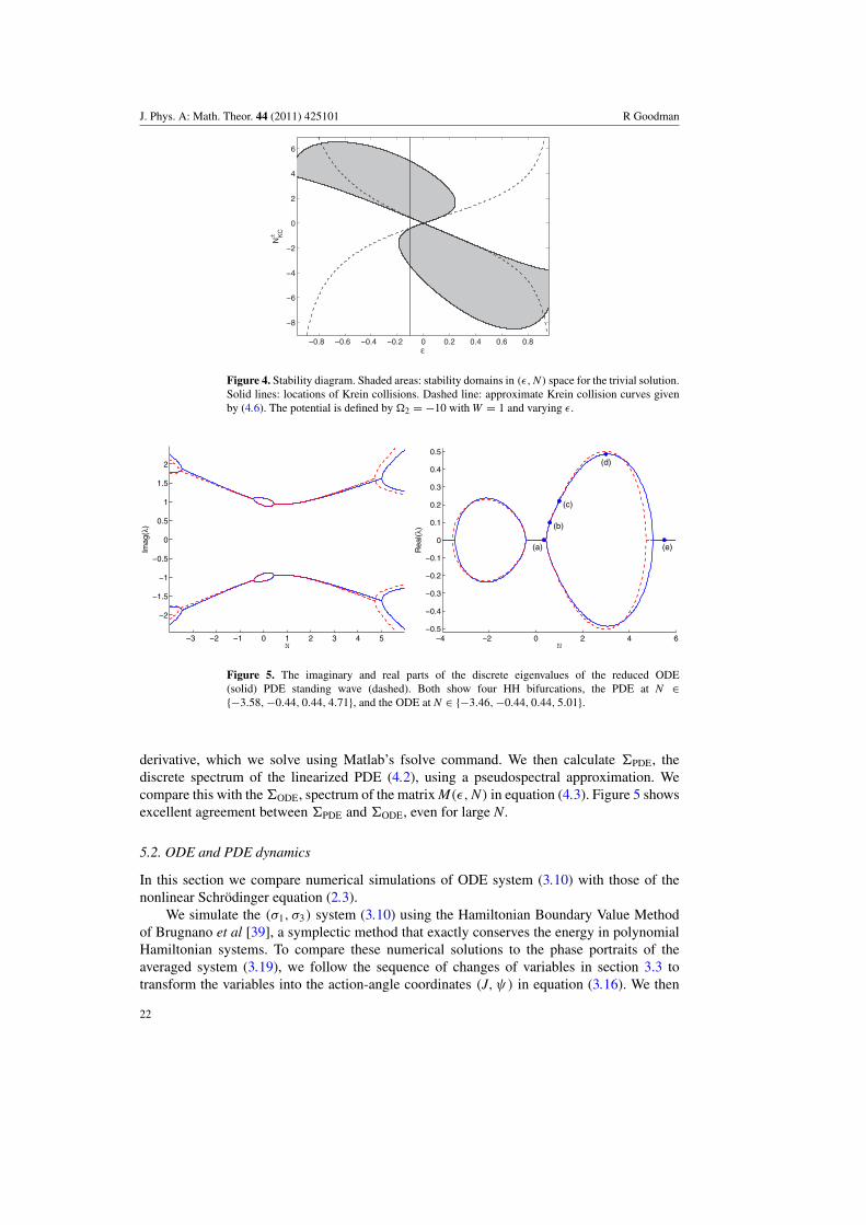
Figure 4. Stability diagram. Shaded areas: stability domains in (ε, N) space for the trivial solution.Solid lines: locations of Krein collisions. Dashed line: approximate Krein collision curves givenby (4.6). The potential is defined by �2 = −10 with W = 1 and varying ε.

−3 −2 −1 0 1 2 3 4 5

−2

−1.5

−1

−0.5

0

0.5

1

1.5

2

N

Imag

(λ)

−4 −2 0 2 4 6−0.5

−0.4

−0.3

−0.2

−0.1

0

0.1

0.2

0.3

0.4

0.5

(a)

(b)

(c)

(d)

(e)

N

Rea

l(λ)

Figure 5. The imaginary and real parts of the discrete eigenvalues of the reduced ODE(solid) PDE standing wave (dashed). Both show four HH bifurcations, the PDE at N ∈{−3.58,−0.44, 0.44, 4.71}, and the ODE at N ∈ {−3.46,−0.44, 0.44, 5.01}.

derivative, which we solve using Matlab’s fsolve command. We then calculate �PDE, thediscrete spectrum of the linearized PDE (4.2), using a pseudospectral approximation. Wecompare this with the �ODE, spectrum of the matrix M(ε, N) in equation (4.3). Figure 5 showsexcellent agreement between �PDE and �ODE, even for large N.

5.2. ODE and PDE dynamics

In this section we compare numerical simulations of ODE system (3.10) with those of thenonlinear Schrodinger equation (2.3).

We simulate the (σ1, σ3) system (3.10) using the Hamiltonian Boundary Value Methodof Brugnano et al [39], a symplectic method that exactly conserves the energy in polynomialHamiltonian systems. To compare these numerical solutions to the phase portraits of theaveraged system (3.19), we follow the sequence of changes of variables in section 3.3 totransform the variables into the action-angle coordinates (J, ψ) in equation (3.16). We then

22

J. Phys. A: Math. Theor. 44 (2011) 425101 R Goodman

compute Poincare sections of (J3, ψ3) on the section ψ1 ≡ 0 mod 2π , which are comparedwith the phase portraits of the system (3.19) in figure 3. For small values of N, the Poincaresections resemble the level sets of the averaged system, with the agreement decreasing forlarger N, parts (a) and (b). As N is increased and new families of periodic orbits appear inthe averaged system, we find Poincare sections lying near tori with the same topology, parts(b)–(d). For larger N, the non-integrability of system (3.10) becomes apparent. We show insubfigure (c), marked with an arrow, one resonant torus that has broken up into an island chainwith five islands. In subfigure (d), the Poincare sections no longer follow the trajectories ofsystem (3.10) well at all.

We next present simulations that demonstrate the dynamics of small perturbations to theantisymmetric standing wave uN2 (x) defined in section 1.2, and to compare these solutions ofNLS/GP (2.3) with approximations constructed from solutions to the (σ1, σ3) system (3.10).To simulate solutions to (2.3), we use a Matlab code written by T Dohnal. It uses fourth-ordercentered differences in space, and an implicit-explicit additive Runge–Kutta method for timestepping [40] and, most importantly for long-term simulation, uses perfectly matched layers(PML) to handle the outgoing radiation [41].

For the NLS simulations, we begin with the same values of σ1 and σ3 as above, andcompute σ2 = ρ = (

1 − σ 21 − σ 2

3

)1/2. From these, we construct the initial conditions with

u(x, 0) = ∑3j=1 σ jUj(x).We then post-process these PDE simulations to compare them with

ODE system (3.10). First we numerically compute the projections (3.2), giving parametersc j(t). Dividing c j by the phase of c2(t) give values analogous to σ j and ρ(t). We then repeatthe steps outlined above to obtain variables akin to (J3, ψ3).

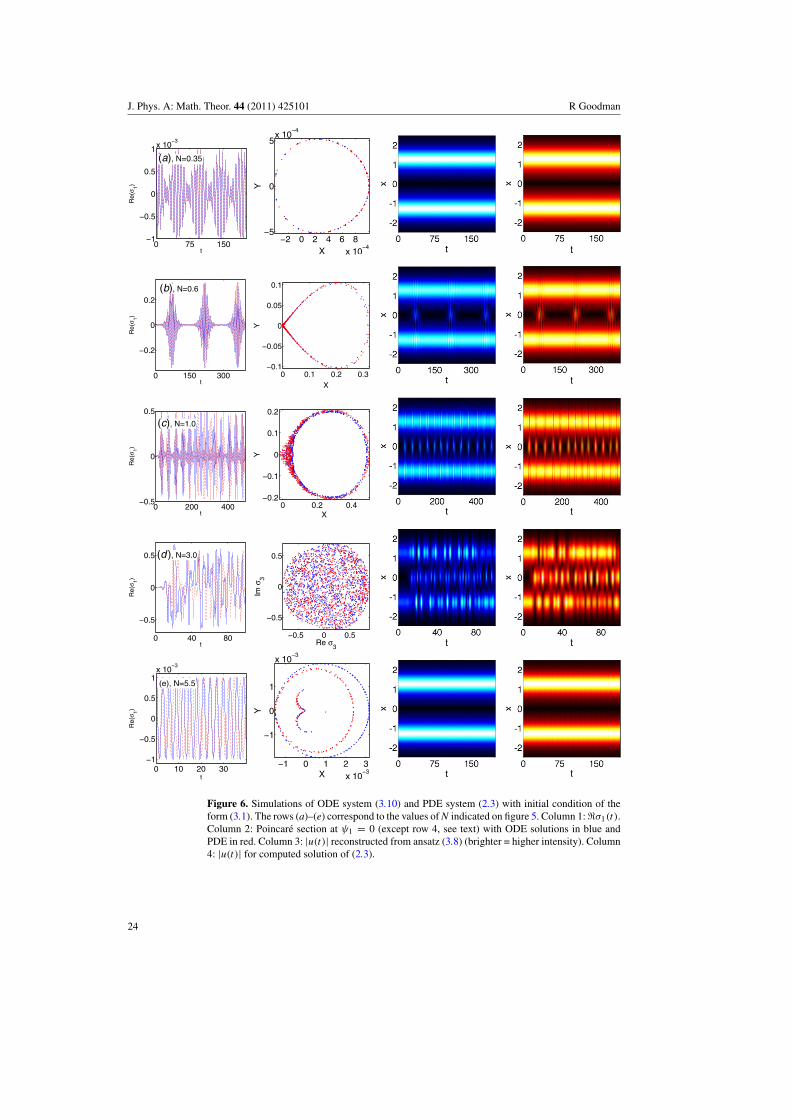
Numerical experiments for the five values of N marked in figure 5 are displayed infigure 6. In all cases the initial conditions used are σ1 = σ3 = 10−5. The first column containstime series of �σ1 for numerical solutions to (2.3) and (3.10). The second, a Poincare sectionon ψ1 ≡ 0 mod 2π ; plotted are X = √

J3 cos ψ3 versus Y = √J3 sin ψ3 for simulations of the

same two systems. The third column contains the amplitude |u(x, t)|, reconstructed from anumerical simulation of system (3.10), computed using (3.1) and (3.8). Column four contains|u(x, t)| from direct numeral simulation of NLS/GP, equation (2.3).

In the five computations, we see that (a) for small N < NKC, the solution stays in aneighborhood of zero and oscillates quasiperiodically. (b) For N slightly greater than NKC, thesolution undergoes a sequence of homoclinic bursts, where an oscillatory bright spot growsperiodically in the middle well, taking energy from the two outer wells. (c) For somewhat largerN, the spacing between the bursts becomes irregular, and the Poincare section displays a ‘lacecurtain’ structure typical of Hamiltonian chaos, with very similar structure in the ODE andPDE simulations. (d) For N chosen to maximize the instability, the dynamics is very irregularand fills the energetically accessible region of phase space. The ODE and PDE simulationsseparate exponentially, but display remarkably similar dynamics. (e) For N sufficiently large,the trivial solution is again stable. In simulation (d), we are unable to use ψ1 as a time-likevariable as in (3.18) because it is non-monotonic; see remark 5. We instead display the Poincaresection σ1 ∈ R.

The equilibrium JNO of the averaged equation exists for N > NKC, corresponding to aperiodic orbit of system (3.10). We solve for this periodic orbit numerically, which then canbe used to construct a relative periodic orbit of system (3.4). Using the decomposition (3.1)with the assumption η = 0, we can approximate a quasiperiodic time-dependent field whichshould be shadowed by a solution to (1.1).

This reconstructed field, computed for the parameter value N = 2, is shown in figure 7.The bright spots move around due to constructive and destructive interference between the threeeigenfunctions. The odd symmetry is broken, as the minimum amplitude location meanders

23

J. Phys. A: Math. Theor. 44 (2011) 425101 R Goodman

0 75 150−1

−0.5

0

0.5

1x 10−3

t

Re(

σ 1)

(a), N=0.35

−2 0 2 4 6 8x 10

−4

−5

0

5x 10

−4

XY

0 150 300

−0.2

0

0.2

t

Re(

σ 1)

(b), N=0.6

0 0.1 0.2 0.3−0.1

−0.05

0

0.05

0.1

X

Y

0 200 400−0.5

0

0.5

t

Re(

σ 1)

(c), N=1.0

0 0.2 0.4−0.2

−0.1

0

0.1

0.2

X

Y

0 40 80

−0.5

0

0.5

t

Re(

σ 1)

(d ), N=3.0

−0.5 0 0.5

−0.5

0

0.5

Re σ3

Im σ

3

0 10 20 30−1

−0.5

0

0.5

1x 10

−3

t

Re(

σ 1)

(e), N=5.5

−1 0 1 2 3x 10

−3

−1

0

1

x 10−3

X

Y

Figure 6. Simulations of ODE system (3.10) and PDE system (2.3) with initial condition of theform (3.1). The rows (a)–(e) correspond to the values of N indicated on figure 5. Column 1: �σ1(t).Column 2: Poincare section at ψ1 = 0 (except row 4, see text) with ODE solutions in blue andPDE in red. Column 3: |u(t)| reconstructed from ansatz (3.8) (brighter = higher intensity). Column4: |u(t)| for computed solution of (2.3).

24

J. Phys. A: Math. Theor. 44 (2011) 425101 R Goodman

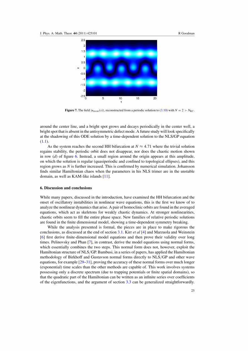
Figure 7. The field |urecon(x)|, reconstructed from a periodic solution to (3.10) with N = 2 > NKC.

around the center line, and a bright spot grows and decays periodically in the center well, abright spot that is absent in the antisymmetric defect mode. A future study will look specificallyat the shadowing of this ODE solution by a time-dependent solution to the NLS/GP equation(1.1).

As the system reaches the second HH bifurcation at N ≈ 4.71 where the trivial solutionregains stability, the periodic orbit does not disappear, nor does the chaotic motion shownin row (d) of figure 6. Instead, a small region around the origin appears at this amplitude,on which the solution is regular (quasiperiodic and confined to topological ellipses), and thisregion grows as N is further increased. This is confirmed by numerical simulation. Johanssonfinds similar Hamiltonian chaos when the parameters in his NLS trimer are in the unstabledomain, as well as KAM-like islands [11].

6. Discussion and conclusions

While many papers, discussed in the introduction, have examined the HH bifurcation and theonset of oscillatory instabilities in nonlinear wave equations, this is the first we know of toanalyze the nonlinear dynamics that arise. A pair of homoclinic orbits are found in the averagedequations, which act as skeletons for weakly chaotic dynamics. At stronger nonlinearities,chaotic orbits seem to fill the entire phase space. New families of relative periodic solutionsare found in the finite dimensional model, showing a time-dependent symmetry breaking.

While the analysis presented is formal, the pieces are in place to make rigorous theconclusions, as discussed at the end of section 3.1. Kirr et al [4] and Marzuola and Weinstein[6] first derive finite-dimensional model equations and then prove their validity over longtimes. Pelinovsky and Phan [7], in contrast, derive the model equations using normal forms,which essentially combines the two steps. This normal form does not, however, exploit theHamiltonian structure of NLS/GP. Bambusi, in a series of papers, has applied the Hamiltonianmethodology of Birkhoff and Gustavson normal forms directly to NLS/GP and other waveequations, for example [29–31], proving the accuracy of these normal forms over much longer(exponential) time scales than the other methods are capable of. This work involves systemspossessing only a discrete spectrum (due to trapping potentials or finite spatial domains), sothat the quadratic part of the Hamiltonian can be written as an infinite series over coefficientsof the eigenfunctions, and the argument of section 3.3 can be generalized straightforwardly.

25

J. Phys. A: Math. Theor. 44 (2011) 425101 R Goodman

These assumptions on the spectrum are also necessary for the applicability of the normalforms over such long time scales. In [32], Bambusi and Cuccagna apply the method to aKlein–Gordon equation in three spatial dimensions with a potential that vanishes at infinity,and so generalize the Birkhoff normal form to systems with a continuous spectrum. This resultapplies only for solutions with very small initial data, where the effect of the nonlinearity is notstrong enough for the bifurcations and strongly nonlinear dynamics that we have discussed.Nonetheless, this is a promising approach for future research.

In the finite dimensional system of approximate equations near a symmetry-breakingbifurcation, derived in [4, 6], it takes one line of algebra to show the existence of the twonew asymmetric solutions that are born when the bifurcation occurs. In system (3.4), theanalysis is not so simple, and the new solution arising from the bifurcation appears, in itssimplest form, as the equilibrium (4.8) of Hamiltonian system (3.19) that corresponds to aperiodic orbit of system with Hamiltonian (3.6). Proving the existence of this periodic orbitis a straightforward application of a paper from the late 1980s by Chow and Kim [33] andwill constitute the first step of a planned program to put the results of the present paper ona more rigorous footing. Beyond that, almost nothing has been proven about the semisimpleindefinite HH bifurcation. One might hope to reproduce some of the many results proven for thegeneric case, but because the semisimple case has higher codimension, the analysis should beharder.

In numerical simulations of this system, we observe Hamiltonian chaotic motion, theunderlying dynamics of which, given by system (3.6) are essentially two degree-of-freedom.Motion of such a system occurs on level sets of the Hamiltonian H which are three-dimensional manifolds in the four-dimensional phase space. Invariant tori in this system aretwo-dimensional subsets of these manifolds. The KAM theorem (or something very similar,see [23]) implies that most of these tori persist when 0 < (N −NKC) � 1. A two-dimensionaltorus separates the three-dimensional manifold, so that trajectories cannot cross from one sideof the torus to the other. This implies that solutions starting near the odd-symmetric relativeequilibria must remain near that point. If the linear system (2.1) is assumed to support a fourtheigenmode, with similar assumptions on the spacing of the eigenvalues, then in this weaklyunstable regime, with six-dimensional phase space, solutions no longer need stay close tothe equilibrium, a process known as Arnol’d diffusion [37]. Further studies are planned toinvestigate this possibility.

We have assumed throughout this paper that the potential V (x) enjoys even spatialsymmetry. The HH bifurcation we discussed depends only on assumptions (S1)–(S4) andnot on this symmetry. Lacking such a symmetry, the finite-dimensional model (3.6) and itsrelative equilibria given in section 4.1 would be significantly more complicated, and the normalform for the HH bifurcation might no longer be semisimple. An interesting question would beto see how the dynamics change in the face of such asymmetry.

Finally, when considered as a model for an optical waveguide, the system studiedhere should be straightforward to implement in a laboratory setting. Discussions areunderway to make this happen and will form the basis of an experimental line ofresearch.

Acknowledgments

Thanks to Denis Blackmore, Eduard Kirr, Elie Shlizerman, David Trubatch and MichaelWeinstein for useful discussions, Richard Kollar and Arnd Scheel for useful comments inresponse to a presentation, and Jeremy Marzuola for a careful reading of the manuscript.Thanks to the referees for their many suggestions, which have significantly improved this

26

J. Phys. A: Math. Theor. 44 (2011) 425101 R Goodman

paper. The code used to simulate PDE solutions is by Tomas Dohnal. RHG was supported byNSF-DMS-0807284. This work was completed while the author was on sabbatical at Technion,the Israel Institute of Technology. He thanks them for their hospitality.

Appendix. Construction of the linear potential V (x)

Most other studies about the dynamics and stability of nonlinear PDEs with multi-wellpotentials have constructed the potential as the sum of several simpler potentials as in equations(1.3) and (1.4) [4, 6, 7, 5, 8]. This construction provides, very simply, families of potentialswith nearly-multiple eigenvalues, but does not allow the control needed to construct potentialssatisfying the assumptions (S1)–(V3).

Another way to proceed is to use inverse scattering methods to construct a reflectionlesspotential with prescribed eigenvalues � j = −κ2

j , j = 1 . . . n. This process yields a potentialthat is unique except for n integrating factors ξ j, which can be chosen uniquely to makeV (x)

satisfy assumption (V3). The solution is a two-soliton solution of the Korteweg–de Vriesequation [42]. This solution is most easily constructed using the Darboux transformation,which is very similar to the Backlund transformation, except that it yields not only thepotential, but also its eigenvectors, which is useful in what follows [43, 44]. When n = 2, thegeneral formula for this two-soliton is

V (x) = 4(κ2

2 − κ21

)(κ2

2 cosh 2κ1x + κ21 cosh 2κ2x

)((κ1 − κ2) cosh (κ2 + κ1)x + (κ1 + κ2) cosh (κ1 − κ2)x)2

(A.1)

with κ1 > κ2 > 0. This has (un-normalized) ground state and excited states

U1 = cosh κ2x

(κ1 − κ2) cosh (κ1 + κ2)x + (κ1 + κ2) cosh (κ1 − κ2)x

and U2 = sinh κ1x

(κ1 − κ2) cosh (κ2 + κ1)x + (κ1 + κ2) cosh (κ1 − κ2)x

and frequencies � j = −κ2j . When κ1 = 2 and κ2 = 1, this potential reduces to the familiar

initial condition for the KdV two-soliton V (x) = −6sech2x with frequencies �1 = −4 and�2 = −1. Choosing κ1 = √

1 + ε and κ2 = √1 − ε, with 0 < ε � 1, the potential (A.1) takes

the form of dual-well potential, very similar to that studied by Kirr et al, but with closed-formeigenvalues and eigenfunctions.

The potential V (x) constructed as above with three frequencies and satisfying assumption(V3) is similar in form to that in (A.1), but with ten terms in the numerator and fourin the denominator. This solution is given in the supplementary materials (available atstacks.iop.org/JPA/44/425101/mmedia), as well as a Mathematica notebook of its derivation.As the spacings between the frequencies are chosen to approach zero, the potential V (x)

asymptotically approaches the superposition of three identical potentials with large spacing,as studied by Kapitula et al [8].

References

[1] Boyd R W 2008 Nonlinear Optics 3rd edn (New York: Academic)[2] Newell A C and Moloney J V 2003 Nonlinear Optics (Advanced Book Program) (Boulder, CO: Westview Press)[3] Pitaevskii L and Stringari S 2003 Bose–Einstein Condensation (Oxford: Oxford University Press)[4] Kirr E W, Kevrekidis P G, Shlizerman E and Weinstein M I 2008 SIAM J. Math. Anal. 40 566–604[5] Sacchetti A 2009 Phys. Rev. Lett. 103 194101[6] Marzuola J L and Weinstein M I 2010 DCDS-A 28 1505–54[7] Pelinovsky D and Phan T 2011 arXiv:1101.5402v1

27

J. Phys. A: Math. Theor. 44 (2011) 425101 R Goodman

[8] Kapitula T, Kevrekidis P G and Chen Z 2006 SIAM J. Appl. Dyn. Syst. 5 598–633[9] Mayteevarunyoo T, Malomed B A and Dong G 2008 Phys. Rev. A 78 53601

[10] Kapitula T and Kevrekidis P G 2005 Chaos 15 037114[11] Johansson M 2004 J. Phys. A: Math. Gen. 37 2201[12] Kapitula T, Kevrekidis P G and Malomed B A 2001 Phys. Rev. E 63 036604[13] Morgante A M, Johansson M, Kopidakis G and Aubry S 2000 Phys. Rev. Lett. 85 550–3[14] Panda S, Lahiri A, Roy T K and Lahiri A 2005 Physica D 210 262–83[15] Kevrekidis P G, Frantzeskakis D J, Malomed B A, Bishop A and Kevrekidis I 2003 New J. Phys. 5 64[16] Kevrekidis P G, Malomed B A, Frantzeskakis D J, Bishop A R, Nistazakis H E and Carretero-Gonzalez R 2005

Math. Comput. Simulat. 69 334–45[17] Li L, Li Z, Malomed B A and Mihalache D 2005 Phys. Rev. A 72 033611[18] Nistazakis H, Frantzeskakis D J and Kevrekidis P G 2007 Phys. Rev. A 76 063603[19] Theocharis G, Weller A, Ronzheimer J P, Gross C, Oberthaler M K, Kevrekidis P G and Frantzeskakis D J 2010

Phys. Rev. A 81 063604[20] van der Meer J-C 1985 The Hamiltonian Hopf Birfurcation (Lecture Notes in Mathematics vol 1160) (Berlin:

Springer)[21] Cushman R and Rod D L 1982 Physica D 6 105–12[22] Gaivao J P and Gelfreich V 2011 Nonlinearity 24 677[23] Dullin H R and Ivanov A V 2005 Phys. D 201 27–44[24] Kapitula T, Kevrekidis P G and Sandstede B 2004 Phys. D 195 263–82[25] Kapitula T, Kevrekidis P G and Sandstede B 2005 Phys. D 201 199–201[26] Kapitula T, Kevrekidis P G and Carretero-Gonzalez R 2007 Phys. D 233 112–37[27] Hislop P D and Sigal I M 1996 Introduction to Spectral Theory: With Applications to Schrodinger Operators

(Applied Mathematical Sciences) (Berlin: Springer)[28] Wiggins S 2003 Introduction to Applied Nonlinear Dynamical Systems and Chaos 2nd edn (Berlin: Springer)[29] Bambusi D 2008 Hamiltonian Dynamical Systems and Applications (NATO Science for Peace and Security

Series B: Physics and Biophysics) (Dordrecht: Springer) pp 213–47[30] Bambusi D 1999 Math. Z. 230 345–87[31] Bambusi D and Sacchetti A 2007 Commun. Math. Phys. 275 1–36[32] Bambusi D and Cuccagna S 2009 arXiv:0908.4548[33] Chow S-N and Kim Y-I 1988 Applicable Anal. 31 163–99[34] Lahiri A and Roy M S 2001 Int. J. Nonlinear Mech. 36 787–802[35] MacKay R 1987 Hamiltonian Dynamical Systems ed J M R MacKay (Bristol: Hilger) pp 137–53 (available at

http://books.google.com/books?id=a1ToPs9iZlEC)[36] Luzzatto-Fegiz P and Williamson C H K 2011 Proc. R. Soc. A 467 1164–85[37] Arnol’d V I, Kozlov V V and Neishtadt A I 1997 Mathematical Aspects of Classical and Celestial Mechanics

2nd edn (Berlin: Springer)[38] Guckenheimer J and Holmes P 1983 Nonlinear Oscillations, Dynamical Systems, and Bifurcations of Vector

Fields (New York: Springer)[39] Brugnano L, Iavernaro F and Trigiante D 2009 AIP Conf. Proc. 1168 715–8[40] Kennedy C A and Carpenter M H 2003 Appl. Numer. Math. 44 139–81[41] Dohnal T and Hagstrom T 2007 J. Comput. Phys. 223 690–710[42] Drazin P G and Johnson R S 1993 Solitons: An Introduction (Cambridge: Cambridge University Press)[43] Ablowitz M J, Prinari B and Trubatch A D 2004 Discrete and Continuous Nonlinear Schrodinger Systems

(Cambridge: Cambridge University Press)[44] Matveev V B and Salle M A 1991 Darboux Transformations and Solitons (Berlin: Springer)

28