1

Hamiltonian Dynamics from

Lie–Poisson Brackets

Jean-Luc Thiffeault

Department of Applied Physics and Applied Mathematics

Columbia University

http://plasma.ap.columbia.edu/~jeanluc

12 February 2002

2

Overview

• Many physical systems have a Hamiltonian formulation in

terms of Lie–Poisson brackets obtained from Lie algebra

extensions.

• This is true for finite-dimensional (e.g., heavy top, Kida

vortex) and infinite-dimensional (Euler’s equation with an

advected scalar, reduced magnetohydrodynamics) systems.

• We the classify low-order extensions, thus showing that there

are only a small number of independent normal forms. We

make use of Lie algebra cohomology to achieve this.

• We give a simple example of a mechanical system with

nontrivial Lie–Poisson structure, the Twisted Top.

3

Noncanonical Hamiltonian Formulation

A system of equations has a noncanonical Hamiltonian formulation

if it can be written in the form

ξλ =

ξλ , H

where H is a Hamiltonian functional, and ξλ(x, t) or ξλi (t)

represents a vector of state variables.

(angular momentum, vorticity, temperature, . . . )

The Poisson bracket , is antisymmetric and satisfies the Jacobi

identity,

F , G ,H + G , H ,F + H , F ,G = 0.

Jacobi tells us that there exist local canonical coordinates.

4

The Lie–Poisson Bracket

We define the Lie–Poisson bracket for one field variable ξ as

F ,G :=

⟨

ξ ,

[

δF

δξ,δG

δξ

]⟩

In infinite dimensions, the pairing 〈·〉 is an integral over a 2-D

spatial domain, and the inner bracket is the 2-D Jacobian,

[ a , b ] =∂a

∂x

∂b

∂y−∂b

∂x

∂a

∂y.

For finite-dimensional systems, the inner bracket we use is

[ a , b ] = a× b,

where our state variables a and b are now 3-vectors; the pairing is a

dot product of vectors.

5

Example: The 2-D Euler Equation

Consider the Hamiltonian

H[ω] = 12

∫

Ω

|∇φ(x, t)|2 d2x,δH

δω= −φ,

where φ is the streamfunction and ω = ∇2φ is the vorticity.

Inserting this into the Lie–Poisson bracket, we have

ω(x, t) = ω ,H =

∫

Ω

ω(x′, t)

[

δω(x, t)

δω(x′, t),

δH

δω(x′, t)

]

d2x′

=

∫

Ω

ω(x′, t) [ δ(x − x′) ,−φ(x′, t) ] d2x′ = [ω(x, t) , φ(x, t) ]

which is Euler’s equation for the 2-D ideal fluid.

Similarly, the finite-dimensional Lie–Poisson bracket generates

Euler’s equation for the dynamics of the rigid body. The dynamical

variable ξ is then the angular momentum vector `.

6

Lie–Poisson Bracket Extensions

These “Euler equation” brackets act as our building block.

We wish to describe a Lie–Poisson system consisting of several

state variables ξλ. The most general linear combination of

one-variable brackets is

F ,G = Wλµν

⟨

ξλ ,

[

δF

δξµ,δG

δξν

]⟩

where repeated indices are summed from 0 to n. W is constant and

transforms like a 3-tensor under linear transformations of ξ; it

determines the structure of the bracket.

We call this structure an extension of the one-variable bracket.

7

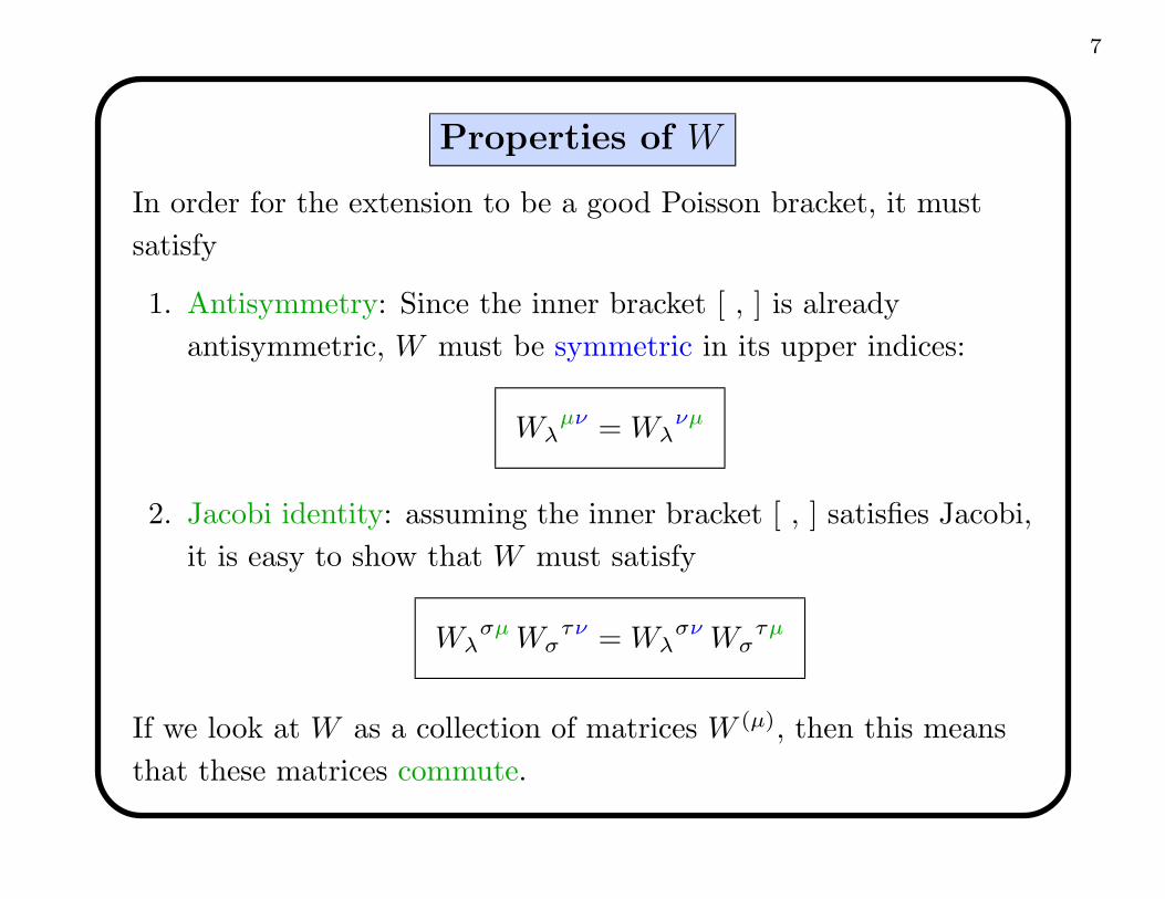
Properties of W

In order for the extension to be a good Poisson bracket, it must

satisfy

1. Antisymmetry: Since the inner bracket [ , ] is already

antisymmetric, W must be symmetric in its upper indices:

Wλµν = Wλ

νµ

2. Jacobi identity: assuming the inner bracket [ , ] satisfies Jacobi,

it is easy to show that W must satisfy

WλσµWσ

τν = Wλσν Wσ

τµ

If we look at W as a collection of matrices W (µ), then this means

that these matrices commute.

8

Example: Compressible Reduced MHD

The four-field model derived by Hazeltine et al. (1987) for 2-D

compressible reduced MHD (CRMHD) has a Lie–Poisson structure.

ω = [ω , φ ] + [ψ , J ] + 2 [ p , x ]

v = [ v , φ ] + [ψ , p ] + 2βe [x , ψ ]

p = [ p , φ ] + βe [ψ , v ]

ψ = [ψ , φ ] ,

The Hamiltonian functional is the total energy,

H[ω, v, p, ψ] =1

2

∫

Ω

|∇φ|2 + v2 +

(p− 2βe x)2

βe+ |∇ψ|2

d2x.

(ξ0, ξ1, ξ2, ξ3) = (ω, v, p, ψ)

9

The W tensor for CRMHD

W (0) =

1 0 0 0

0 1 0 0

0 0 1 0

0 0 0 1

, W (1) =

0 0 0 0

1 0 0 0

0 0 0 0

0 0 −βe 0

,

W (2) =

0 0 0 0

0 0 0 0

1 0 0 0

0 −βe 0 0

, W (3) =

0 0 0 0

0 0 0 0

0 0 0 0

1 0 0 0

.

It is easily verified that these commute, so that the Jacobi identity

holds. (Note the lower-triangular structure.)

10

Since W is a 3-tensor, we can represent it as a cube:

The vertical axis is the lower index of Wλµν , with the origin at the

top rear. The two horizontal axes are the symmetric upper indices.

The red cubes are −βe terms, the blue cubes are unity.

(Symmetric when viewed from the top.)

11

Classification of Extensions

How many independent extensions are there?

The answer amounts to finding normal forms for W , independent

under coordinate transformations.

Threefold process:

1. Decomposition into a direct sum.

2. Transforming the matrices W (µ) to lower-triangular form.

3. Finally, the hard part is to use Lie algebra cohomology to

achieve the classification (almost).

12

Classification 1: Direct Sum Structure

A set of commuting matrices, by a coordinate transformation, can

always be put in block-diagonal form. The 3-tensor W then looks

like:

Each “step” corresponds to a degenerate eigenvalue of the W (µ).

13

Then, the symmetry of the upper indices of W implies the

following structure:

We can focus on each block independently.

14

Classification 2: Lower-triangular Form

We focus on a single block, and thus assume that the W (µ) have

(n+ 1)-fold degenerate eigenvalues.

A set of commuting matrices can always be put into

lower-triangular form by a coordinate transformation.

Once we do this, by the symmetry of the upper indices of W it is

easy to show that

only the eigenvalue of W (0) can be nonzero.

Furthermore, if it is nonzero it can be rescaled to unity. We assume

this is the case.

15

The most general form of W for an extension is thus

The red cubes form a solvable subalgebra, and are constrained by

the commutation requirement. The blue cubes represent unit

elements.

16

Classification 3: Cohomology

The problem of classifying extensions is reduced to classifying the

solvable (red) part of the extension. This is achieved by the

techniques of Lie algebra cohomology.

Cohomology gives us a class of linear transformations that preserve

the lower-triangular structure of the extensions.

The parts of the extension that can be removed (i.e., made to

vanish) by such transformations are called coboundaries.

What is left are nontrivial cocycles.

(Cohomology does not quite get it all. . . )

17

Pure Semidirect Sum

A common form for the bracket is the semidirect sum (SDS), for

which the solvable part of W vanishes:

Note that CRMHD does not have a semidirect sum

structure because of its extra nonzero blocks equal

to −βe (a cocycle).

18

Leibniz Extension

The opposite extreme to the pure semidirect sum is the case for

which none of the W (µ) vanishes. Then W must have the structure

This is called the Leibniz extension. All the cubes, red and blue,

are equal to unity.

19

In between these two extreme cases, there are other possible

extensions, including the CRMHD bracket.

Order Number of extensions

1 1

2 1

3 2

4 4

5 9

None of these normal forms contains any free parameter!

(Do not expect this to be true at order 6 and beyond.)

[Thiffeault and Morrison, Physica D 136, 205 (2000)]

20

The Twisted Top

The charged heavy top has a semidirect structure. The simplest

nonsemidirect extension we can make corresponds to the Leibniz

extension:

H(`,α,β) = 12` · ω + α · a + β · b

˙ = ` × ω + α × a + β × b,

α = α × ω + εβ × a,

β = β × ω.

Same Hamiltonian as charged heavy top, but different Lie–Poisson

bracket → cocycle.

[Thiffeault and Morrison, Physics Letters A 283, 335 (2001)]

21

Invariants

The twisted top has three Casimir invariants,

C1 = ‖α‖2

+ 2ε ` · β, C2 = α · β, C3 = ‖β‖2.

The number of degrees of freedom is thus (9 − 3)/2 = 3.

For the Lagrange (symmetric) case,

I1 = I2, α = (0, 0, α3), β = 0,

in addition to the energy there are two more invariants,

`3 and P = ` · α + ε I1a3 β3 ,

so that the symmetric case is integrable, as for the heavy top.

22

This dynamical system remains largely unexplored:

• Equilibria, periodic orbits, stability. . .

• Bifurcations of Poincare sections, a la Dullin et al.

(Canonical coordinates)

• Kovalevskaya case? Not obviously, but maybe nearby. . .

(Painleve analysis)

• Physical relevance? (Underwater vehicles?)

• Is there a signature of the cocycle in the dynamics?

• Twisted fluid?

23

Poincare Section

-1 -0.75 -0.5 -0.25 0 0.25 0.5 0.75 10

1

2

3

4

5

6

PSfrag replacements

sinφ

pφ2

ε = 0.5

ε = 0.11

ε = 0.01