HAL Id: hal-01446063https://hal.archives-ouvertes.fr/hal-01446063

Submitted on 25 Jan 2017

HAL is a multi-disciplinary open accessarchive for the deposit and dissemination of sci-entific research documents, whether they are pub-lished or not. The documents may come fromteaching and research institutions in France orabroad, or from public or private research centers.

L’archive ouverte pluridisciplinaire HAL, estdestinée au dépôt et à la diffusion de documentsscientifiques de niveau recherche, publiés ou non,émanant des établissements d’enseignement et derecherche français ou étrangers, des laboratoirespublics ou privés.

Estimation of the joint distribution of random effects fora discretely observed diffusion with random effects

Maud Delattre, Valentine Genon-Catalot, Catherine Larédo

To cite this version:Maud Delattre, Valentine Genon-Catalot, Catherine Larédo. Estimation of the joint distribution ofrandom effects for a discretely observed diffusion with random effects. 2017. hal-01446063

Estimation of the joint distribution of random effects for a

discretely observed diffusion with random effects.

Maud Delattre1, Valentine Genon-Catalot2 and Catherine Larédo3∗

1 AgroParisTech, France2 UMR CNRS 8145, Laboratoire MAP5, Université Paris Descartes, Sorbonne Paris Cité, France

3 Laboratoire MaIAGE, I.N.R.A. and LPMA, Université Denis Diderot, UMR CNRS 7599.

January 25, 2017

Abstract

Mixed effects models are popular tools for analyzing longitudinal data from several individuals si-multaneously. Individuals are described by N independent stochastic processes (Xi(t), t ∈ [0, T ]),i = 1, . . . , N , defined by a stochastic differential equation with random effects. We assume that thedrift term depends linearly on a random vector Φi and the diffusion coefficient depends on anotherlinear random effect Ψi. For the random effects, we consider a joint parametric distribution leading toexplicit approximate likelihood functions for discrete observations of the processes Xi on a fixed timeinterval. The asymptotic behaviour of the associated estimators is studied when both the number ofindividuals and the number of observations per individual tend to infinity. The estimation methodsare investigated on simulated and real neuronal data.

Key Words: asymptotic properties, discrete observations, estimating equations, parametric inference,random effects models, stochastic differential equations.

1 Introduction

Mixed effects models are popular tools for analyzing longitudinal data from several individuals simulta-neously. In these models, the individuals are described by the same structural model and the inclusionof some random effects enables the description of the inter-individual variability which is inherent to thedata (see Pinheiro and Bates (2000) for instance). The qualification "mixed-effects" comes from the factthat these models often include two kinds of parameters: the fixed effects that are common to all indi-viduals and the random effects that vary from one individual to another according to a given probabilitydistribution. Such models are especially suited in the biomedical field where typical experiments oftenconsist of repeated measurements on several patients or experimental animals. In stochastic differentialequations with mixed effects (SDEMEs), the structural model is a set of stochastic differential equations.The use of SDEMEs is comparatively recent. It has first been motivated by pharmacological applications(see Ditlevsen and De Gaetano (2005), Donnet and Samson (2008), Delattre and Lavielle (2013), Leanderet al. (2015), Forman and Picchini (2016) and many others) but also neurobiological ones (as in Dion(2016) for example). The main issue in mixed-effects models as well as in SDEMEs is the estimation

∗Corresponding authorEmail addresses: maud.delattre@agroparistech.fr (Maud Delattre), valentine.genon-catalot@parisdescartes.fr (ValentineGenon-Catalot), catherine.laredo@jouy.inra.fr (Catherine Larédo)

1

of the parameters of the distribution of the random effects. It is often difficult in practice due to theuntractable likelihood function. In the SDEMEs framework, many methods have now been proposed.In Ditlevsen and De Gaetano (2005), the special case of a mixed-effects Brownian motion with drift istreated. For general models, methods are based on various numerical approximations of the likelihood(Picchini et al. (2010), Picchini and Ditlevsen (2011), Delattre and Lavielle (2013)). For what concernsthe exact likelihood approach or explicit estimating equations, the main contributions to our knowledgeare from Delattre et al. (2013), Delattre et al. (2015) and Delattre et al. (2016). In this paper, we ex-tend the framework of these three papers, considering discrete observations adding simultaneous randomeffects in the drift and diffusion coefficients by means of a joint parametric distribution. The problem ofestimating simultaneously the distributions of random effects in the drift and in the diffusion coeffcienthas never been studied theoretically to our knowledge.More precisely, we consider N real valued stochastic processes (Xi(t), t ≥ 0), i = 1, . . . , N , with dynamicsruled by the following random effects stochastic differential equation (SDE):

dXi(t) = Φ′ib(Xi(t))dt+ Ψiσ(Xi(t)) dWi(t), Xi(0) = x, i = 1, . . . , N, (1)

where (W1, . . . ,WN ) are N independent Wiener processes, ((Φi,Ψi), i = 1, . . . N) are N i.i.d. Rd ×(0,+∞)-valued random variables, ((Φi,Ψi), i = 1, . . . , N) and (W1, . . . ,WN ) are independent and x is aknown real value. The functions σ(.) : R → R and b(.) = (b1(.), . . . , bd(.))

′ : R → Rd are known. Thenotation X ′ for a vector or a matrix X denotes the transpose of X. Each process (Xi(t)) representsan individual and the d + 1-dimensional random vector (Φi,Ψi) represents the (multivariate) randomeffect of individual i. In Delattre et al. (2013), the N processes are assumed to be continuously observedthroughout a fixed time interval [0, T ], T > 0 and Ψi = γ−1/2 is non random and known. When Φi followsa Gaussian distribution Nd(µ, γ−1Ω), the exact likelihood associated with (Xi(t), t ∈ [0, T ], i = 1, . . . , N)

is explicitely computed and asymptotic properties of the exact maximum likelihood estimators are derivedunder the asymptotic framework N → +∞. In Delattre et al. (2015), the case of b(.) = 0 and Ψi = Γ

−1/2i

with Γi following a Gamma distribution G(a, λ) is investigated. The processes (Xi(t)) are supposedto be discretely observed on the fixed-length time interval [0, T ] at n times tj = jT/n. With thisparametric distribution for the random effects Ψi, an explicit approximate likelihood is built and theassociated estimators are studied assuming that both the number N of individuals and the number n ofobservations per individual tend to infinity. In Delattre et al. (2016), the previous papers are extendedand improved by considering for model (1) the cases Φi ∼ Nd(µ, γ−1Ω), Ψi = γ−1/2 non random butunknown or Φi = ϕ non random and unknown and Ψi = Γ

−1/2i with Γi following a Gamma distribution.

The joint estimation of respectively (γ,µ,Ω) and (λ, a, ϕ) is studied.Our aim here is to study the case where both Φi and Ψi are random and have a joint parametricdistribution. We assume that each process (Xi(t)) is discretely observed on a fixed-length time interval[0, T ] at n times tj = jT/n. We consider a joint parametric distribution for the random effects (Φi,Ψi)

and estimate the unknown parameters from the observations (Xi(tj), j = 1, . . . , n, i = 1, . . . , N). Wefocus on distributions that give rise to explicit approximations of the likelihood functions so that theconstruction of estimators is easy and their asymptotic study feasible. Joining the two cases of Delattre

2

et al. (2016) in a single one, we assume that (Φi,Ψi) has the following distribution:

Ψi =1

Γ1/2i

, Γi ∼ G(a, λ), and given Γi = γ, Φi ∼ Nd(µ, γ−1Ω). (2)

Thus, Φi and Ψi are dependent and the unknown parameter is ϑ = (λ, a,µ,Ω). Let us stress that,contrary to the common Gaussian assumption for random effects, the marginal distribution of Φi is notGaussian: Φi − µ = Γ

−1/2i ηi, with ηi ∼ Nd(0,Ω), is a Student distribution. We propose two distinct

approximate likelihood functions which yield asymptotically equivalent estimators as both N and thenumber n of observations per individual tend to infinity. We obtain consistent and

√N -asymptotically

Gaussian estimators for all parameters under the condition N/n → 0. We compare the results withestimation for direct observation of the random effects; we also compare the results with the analogousones based on continuous observation of the diffusions sample path.The structure of the paper is the following. Some working assumptions and two approximations of themodel likelihood are introduced in Section 2. Two estimation methods are derived from these approximatelikelihoods in Section 3, and their respective asymptotic properties are studied. Section 4 providesnumerical simulation results for several examples of SDEMEs and illustrates the performances of theproposed methods in practice. Section 5 concerns the implementation on a real neuronal dataset. Someconcluding remarks are given in Section 6. Theoretical proofs are gathered in the Appendix.

2 Approximate Likelihood.

Let (Xi(t), t ≥ 0), i = 1, . . . , N be N real valued stochastic processes ruled by (1). The processes(W1, . . . ,WN ) and the r.v.’s (Φi,Ψi), i = 1, . . . , N are defined on a common probability space (Ω,F ,P)

and we set (Ft = σ(Φi,Ψi,Wi(s), s ≤ t, i = 1, . . . , N), t ≥ 0). The set of assumptions is the same as inDelattre et al. (2016). We assume that:

(H1) The real valued functions x→ bj(x), j = 1, . . . , d and x→ σ(x) are C2 on R with first and secondderivatives bounded by L. The function σ(.) is lower bounded : ∃ σ0 > 0,∀x ∈ R, σ(x) ≥ σ0.

(H2) There exists a constant K such that, ∀x ∈ R, ‖b(x)‖+ |σ(x)| ≤ K.(‖.‖ denotes the Euclidian norm of Rd.)

Assumption (H1) ensures existence and uniqueness of solutions of (1) (see e.g. Delattre et al. (2013)).Under (H1), for i = 1, . . . , N , for all deterministic (ϕ,ψ) ∈ Rd × (0,+∞), the stochastic differentialequation

dXϕ,ψi (t) = ϕ′b(Xϕ,ψ

i (t))dt+ ψσ(Xϕ,ψi (t)) dWi(t), Xϕ,ψ

i (0) = x (3)

admits a unique strong solution process (Xϕ,ψi (t), t ≥ 0) adapted to the filtration (Ft). Moreover, the

stochastic differential equation with random effects (1) admits a unique strong solution adapted to (Ft)such that the joint process (Φi,Ψi, Xi(t), t ≥ 0) is strong Markov and the conditional distribution of(Xi(t)) given Φi = ϕ,Ψi = ψ is identical to the distribution of (3). The processes (Φi,Ψi, (Xi(t), t ≥0)), i = 1, . . . , N are i.i.d.. Assumption (H2) simplifies proofs.The processes (Xi(t)) are discretely observed with sampling interval ∆n on a fixed time interval [0, T ]

3

and we set:∆n = ∆ =

T

n, Xi,n = Xi = (Xi(tj,n), tj,n = tj = jT/n, j = 1, . . . , n). (4)

The canonical space associated with one trajectory on [0, T ] is defined by ((Rd × (0,+∞) × CT ), Pϑ)

where CT denotes the space of real valued continuous functions on [0, T ], Pϑ denotes the distribution of(Φi,Ψi, (Xi(t), t ∈ [0, T ]) and ϑ the unknown parameter. For the N trajectories, the canonical space is∏Ni=1((Rd × (0,+∞)× CT ),Pϑ = ⊗Ni=1Pϑ). Below, the true value of the parameter is denoted ϑ0.

The likelihood of the i-th vector of observations is obtained by computing first the conditional likelihoodgiven Φi = ϕ,Ψi = ψ, and then integrate the result with respect to the joint distribution of (Φi,Ψi). Theconditional likelihood given fixed values (ϕ,ψ), i.e. the likelihood of (Xϕ,ψ

i (tj), j = 1, . . . , n) being notexplicit, is approximated by using the Euler scheme likelihood of (3). Setting ψ = γ−1/2, it is given by:

Ln(Xi,n, γ, ϕ) = Ln(Xi, γ, ϕ) = γn/2 exp [−γ2

(Si,n + ϕ′Vi,nϕ− 2ϕ′Ui,n)], (5)

where

Si,n = Si =1

∆

n∑j=1

(Xi(tj)−Xi(tj−1))2

σ2(Xi(tj−1)), (6)

Vi,n = Vi =

n∑j=1

∆bk(Xi(tj−1))b`(Xi(tj−1))

σ2(Xi(tj−1))

1≤k,`≤d

, (7)

Ui,n = Ui =

n∑j=1

bk(Xi(tj−1))(Xi(tj)−Xi(tj−1))

σ2(Xi(tj−1))

1≤k≤d

. (8)

Then, the unconditional likelihood is obtained integrating with respect to the joint distribution νϑ(dγ, dϕ)

of the random effects (Γi = Ψ−2i ,Φi):

LN,n(ϑ) =

N∏i=1

Ln(Xi,n, ϑ), Ln(Xi,n, ϑ) =

∫Ln(Xi,n, γ, ϕ)νϑ(dγ, dϕ).

In general, this does not lead to a closed-form formula. The joint distribution (2) proposed here allowsto obtain an explicit formula for the above integral. Some additional assumptions are required.

(H3) The matrix Vi(T ) is positive definite a.s., where

Vi(T ) =

(∫ T

0

bk(Xi(s))b`(Xi(s))

σ2(Xi(s))ds

)1≤k,`≤d

. (9)

(H4) The parameter set satisfies, for constants m, c0, c1, `0, `1, α0, α1,‖µ‖ ≤ m, λmax(Ω) ≤ c1, 0 < `0 ≤ λ ≤ `1, 0 < α0 ≤ a ≤ α1,

where λmax(Ω)) denotes the maximal eigenvalue of Ω.

Assumption (H3) ensures that all the components of Φi can be estimated. If the functions (bk/σ2) are

not linearly independent, the dimension of Φi is not well defined and (H3) is not fulfilled. Note that, asn tends to infinity, the matrix Vi,n defined in (7) converges a.s. to Vi(T ) so that, under (H3), for n large

4

enough, Vi,n is positive definite.Assumption (H4) is classically used in a parametric setting. Under (H4), the matrix Ω may be noninvertible which allows including non random effects in the drift term.

2.1 First approximation of the likelihood

Let us now compute the approximate likelihood Ln(Xi,n, ϑ) ofXi,n integrating Ln(Xi,n, γ, ϕ) with respectto the distribution (2). For this, we first integrate Ln(Xi, γ, ϕ) with respect to the Gaussian distributionNd(µ, γ−1Ω). Then, we integrate the result w.r.t. the distribution of Γi. At this point, a difficulty arises.This second integration is only possible on a subset Ei,n(ϑ) precised now. Let Id denote the identitymatrix of Rd and set, for i = 1, . . . , N ,

Ri,n = V −1i,n + Ω = V −1

i,n (Id + Vi,nΩ) = (Id + ΩVi,n)V −1i,n (10)

which is well defined and invertible under (H3). Define

Ti,n(µ,Ω) = (µ− V −1i,n Ui,n)′R−1

i,n(µ− V −1i,n Ui,n)− U ′i,nV −1

i,n Ui,n, (11)

Ei,n(ϑ) = Si,n + Ti,n(µ,Ω) > 0 ; EN,n(ϑ) = ∩Ni=1Ei,n(ϑ). (12)

Proposition 1. Assume that, for i = 1, . . . , N , (Φi,Ψi) has distribution (2). Under (H1)-(H3), anexplicit approximate likelihood for the observation (Xi,n, i = 1, . . . , N) is on the set EN,n(ϑ) (see (12)),

LN,n(ϑ) =

N∏i=1

Ln(Xi,n, ϑ), where (13)

Ln(Xi,n, ϑ) =λaΓ(a+ (n/2))

Γ(a)(λ+Si,n

2 +Ti,n(µ,Ω)

2 )a+(n/2)

1

(det(Id + Vi,nΩ))1/2. (14)

We must now deal with the set EN,n(ϑ). For each i, elementary properties of quadratic variations yieldthat, as n tends to infinity, Si,n/n tends to Γ−1

i in probability. On the other hand, the random matrixVi,n tends a.s. to the integral Vi(T ) and the random vector Ui,n tends in probability to the stochasticintegral

Ui(T ) =

(∫ T

0

bk(Xi(s))

σ2(Xi(s))dXi(s)

)1≤k≤d

. (15)

Therefore Ti,n(µ,Ω)/n tends to 0 (see (11)). This implies that, for all i = 1, . . . , N and for all (θ0, θ),Pϑ0

(Ei,n(ϑ))→ 1 as n tends to infinity. However, we need the more precise result

∀ϑ, ϑ0, Pϑ0(EN,n(ϑ))→ 1.

Moreover, the set on which the approximate likelihood is considered should not depend on ϑ.To this end, let us define, for α > 0, using the notations of (H4),

Mi,n = maxc1 + 2, 2m2(1 + ‖Ui,n‖2) ; Fi,n = Si,n −Mi,n ≥ α√n ; FN,n = ∩Ni=1Fi,n. (16)

5

Lemma 1. Assume (H1)-(H4). For all ϑ satisfying (H4) and all i, we have Fi,n ⊂ Ei,n(ϑ).If a0 > 4 and as N,n→∞, N = N(n) is such that N/n2 → 0, then,

∀ϑ0, Pϑ0(FN,n)→ 1.

Consequently, for all ϑ, Pϑ0( EN,n(ϑ))→ 1 and (13) is well defined on the set FN,n which is independentof ϑ and has probability tending to 1.

2.2 Second approximation of the likelihood

Formulae (13)-(14) suggest another approximation of the likelihood which is simpler and related tothe likelihood functions obtained in Delattre et al. (2013) and Delattre et al. (2015). We give thisapproxmation without being rigorous. The formula is justified a posteriori. We can write:

Ln(Xi,n, ϑ) = L(1)n (Xi,n, ϑ)× L(2)

n (Xi,n, ϑ) (17)

L(1)n (Xi,n, ϑ) = L(1)

n (Xi,n, λ, a) =λaΓ(a+ (n/2))

Γ(a)(λ+Si,n

2 )a+(n/2)

L(2)n (Xi,n, ϑ) =

(λ+Si,n

2 )a+(n/2)

(λ+Si,n

2 +Ti,n(µ,Ω)

2 )a+(n/2)

1

(det(Id + Vi,nΩ))1/2.

The first term L(1)n (Xi,n, ϑ) only depends on (λ, a) and is equal to the approximate likelihood function

obtained in Delattre et al. (2015) for b ≡ 0 and Γi ∼ G(a, λ). For the second term, we have:

logL(2)n (Xi,n, ϑ) = −(a+

n

2) log

(1 +

1

n

Ti,n(µ,Ω)

(2λn +Si,n

n )

)− 1

2log (det(Id + Vi,nΩ)).

As for n tending to infinity, Ti,n(µ,Ω) tends to a fixed limit and Si,n/n tends to Γ−1i , this yields:

logL(2)n (Xi,n, ϑ) ∼ −

(a+ n2 )

n

Ti,n(µ,Ω)

(2λn +Si,n

n )− 1

2log (det(Id + Vi,nΩ))

∼ − n

2Si,nTi,n(µ,Ω)− 1

2log (det(Id + Vi,nΩ)).

Now, the above expression only depends on (µ,Ω). Morevover, as the term U ′i,nV−1i,n Ui,n in Ti,n(µ,Ω)

does not contain unknown parameters, we can forget it and set:

V n(Xi,n, ϑ) = V (1)n (Xi,n, λ, a) + V (2)

n (Xi,n,µ,Ω) (18)

6

with

V (1)n (Xi,n, λ, a) = a log λ− log Γ(a)− (a+

n

2) log (λ+

Si,n2

) + log Γ(a+ (n/2))

V (2)n (Xi,n,µ,Ω) = − n

2Si,n(µ− V −1

i,n Ui,n)′R−1i,n(µ− V −1

i,n Ui,n)− 1

2log (det(Id + Vi,nΩ))

and define the second approximation for the log-likelihood: V N,n(ϑ) =∑Ni=1 V n(Xi,n, ϑ). Thus, estima-

tors of (λ, a) and (µ,Ω) can be computed separately.

3 Asymptotic properties of estimators.

In this section, we study the asymptotic behaviour of the estimators based on the two approximatelikelihood functions of the previous section. A natural question arises which concerns the comparisonwith the estimation when direct observation of an i.i.d. sample (Φi,Γi), i = 1, . . . , N is available (detailsare given in Section 8.3).

3.1 Estimation based on the first approximation of the likelihood

We study the estimation of ϑ = (λ, a,µ,Ω) using the approximate likelihood LN,n(ϑ) given in Proposition1 on the set FN,n studied in Lemma 1 (see (13), (14), (16)).Let

Zi,n(a, λ,µ,Ω) = Zi =λ+ (Si,n/2) + (Ti,n(µ,Ω)/2)

a+ n/2. (19)

By (H4), using notations (16), we have λ + Si,n/2 + Ti,n(µ,Ω)/2 ≥ (Si,n −Mi,n)/2. On the set Fi,n,Zi,n > α/(

√n+ 2(α1/

√n)) > 0 where α1 is defined in (H4). Instead of considering logLn(Xi, ϑ) on Fi,n,

to define a contrast, we replace logZi,n by 1Fi,nlogZi,n and set UN,n(ϑ) =

∑Ni=1 Un(Xi, ϑ), with

Un(Xi,n, ϑ) = a log λ− log Γ(a) + log Γ(a+ (n/2))− (a+ (n/2)) log(a+ (n/2))

−1

2log det(Id + Vi,nΩ)− (a+ (n/2))1Fi,n

logZi,n.

Define the gradient vectorGN,n(ϑ) = ∇ϑUN,n(ϑ) (20)

We consider the estimators defined by the estimating equation:

GN,n(ϑN,n) = 0. (21)

To investigate their asymptotic behaviour, we need to prove that Zi,n defined in (19) is close to Γ−1i and

that 1Fi,nZ−1i,n is close to Γi. For this, we introduce the random variable

S(1)i,n = S

(1)i = Ψ2

i

n∑j=1

(Wi(tj)−Wi(tj−1))2

∆=

1

ΓiC

(1)i,n (22)

7

which corresponds to Si,n when b(.) = 0, σ(.) = 1. Then, we split Zi,n−Γ−1i into Zi,n−

S(1)i,n

n +S

(1)i,n

n −Γ−1i and

study successively the two terms. The second term has explicit distribution as C(1)i,n has χ2(n) distribution

and is independent of Γi. The first term is treated below. We proceed analogously for 1Fi,nZ−1i,n − Γi

intoducing n/S(1)i,n .

From now on, for simplicity of notations, we consider the case d = 1 (univariate random effect in the drift,i.e. µ = µ, ω2 = Ω). The case of d > 1 does not present any additional difficulty. Let ϑ = (λ, a, µ, ω2).

Lemma 2. For all p ≥ 1, we have

Eϑ

(∣∣∣∣∣Zi,n − S(1)i,n

n

∣∣∣∣∣p

|Ψi = ψ,Φi = ϕ

).

1

np(1 + ϕ2p + ψ2p + ψ4p + ϕ2pψ2p),

Eϑ

([

∣∣∣∣∣Z−1i,n −

n

S(1)i,n

∣∣∣∣∣p

1Fi,n]|Ψi = ψ,Φi = ϕ

).

1

np(1 + (1 + ϕ2p)(ψ−2p + ψ−4p) + ϕ4p + ψ4p + ϕ4pψ−4p).

Using (7),(8), we set

Ai,n =Ui,n − µVi,n1 + ω2Vi,n

and Bi,n =Vi,n

1 + ω2Vi,n. (23)

Let ψ(u) = Γ′(u)Γ(u) denote the di-gamma function and F c denote the complementary set of F . We obtain

(see (19)):

∂UN,n

∂λ(ϑ) =

N∑i=1

(aλ− Z−1

i,n 1Fi,n

),

∂UN,n

∂a(ϑ) = N (ψ(a+ n/2)− log (a+ n/2)− ψ(a) + log λ)−

N∑i=1

(1Fi,n

logZi,n − 1F ci,n

),

∂UN,n

∂µϑ) = −1

2

N∑i=1

1Fi,nZ−1i,n

∂

∂µTi,n(µ, ω2) =

N∑i=1

1Fi,nZ−1i,nAi,n,

∂UN,n

∂ω2ϑ) = −1

2

N∑i=1

(Vi,n

1 + ω2Vi,n+ 1Fi,n

Z−1i,n

∂

∂ω2Ti,n(µ, ω2)

)=

1

2

N∑i=1

(1Fi,nZ

−1i,nA

2i,n −Bi,n

).

Using (9),(15), we set

Ai(T ;µ, ω2) =Ui(T )− µVi(T )

1 + ω2Vi(T )and Bi(T ;ω2) =

Vi(T )

1 + ω2Vi(T )(24)

and

J(ϑ) =

(EϑΓ1B1(T ;ω2) EϑΓ1A1(T ;µ, ω2)B1(T ;ω2)

EϑΓ1A1(T ;µ, ω2)B1(T ;ω2) Eϑ(Γ1A

21(T ;µ, ω2)B1(T ;ω2)− 1

2B21(T ;ω2)

) ) . (25)

Denote

I0(λ, a) =

(aλ2 − 1

λ

− 1λ ψ′(a)

)(26)

the Fisher information matrix associated with the direct observation (Γ1, . . . ,ΓN ) (see Section 8.3). Wenow state:

8

Theorem 1. Assume (H1)-(H4), a > 4, and that n and N = N(n) tend to infinity. Then, for all ϑ,

• If N/n2 → 0, N−1/2(∂UN,n

∂λ (ϑ),∂UN,n

∂a (ϑ))′

converges in distribution under Pϑ to the Gaussian lawN2(0, I0(λ, a)).

• If N/n → 0, N−1/2(∂UN,n

∂ϑi(ϑ), i = 1, . . . , 4

)′converges in distribution under Pϑ to N4(0,J (ϑ))

where

J (ϑ) =

(I0(λ, a) 0

0 J(ϑ)

)and the matrix J(ϑ) defined in (25) is the covariance matrix of the vector(

Γ1A1(T ;µ, ω2)12 (Γ1A

21(T, µ, ω2)−B1(T ;ω2))

). (27)

• Define the opposite of the Hessian of UN,n(ϑ) by JN,n(ϑ) = (− ∂2

∂ϑi∂ϑjUN,n(ϑ))i,j=1,...,4. Then, if

a > 6, as n and N = N(n) tend to infinity, N−1JN,n(ϑ) converges in Pϑ-probability to J (ϑ).

For the proof, we use that Ai,n (resp. Bi,n) converges to Ai(T ;µ, ω2) (resp. Bi(T ;ω2)) as n tends toinfinity and that Z−1

i,n1Fi,nis close to Γi for large n. Note that I0(λ, a) is invertible for all (λ, a) ∈ (0,+∞)2

(see Section 8.3). We conclude:

Theorem 2. Assume (H1)-(H4), a0 > 6, that n and N = N(n) tend to infinity with N/n→ 0 and thatJ(ϑ0) is invertible. Then, with probability tending to 1, a solution ϑN,n to (21) exists which is consistentand such that

√N(ϑN,n − ϑ0) converges in distribution to N4(0,J−1(ϑ0)) under Pϑ0

for all ϑ0.For the first two components, the constraint N/n2 → 0 is enough.

The proof of Theorem 2 is deduced standardly from the previous theorem and omitted.Let us stress that the estimators of (λ, a) are asymptotically equivalent to the exact maximum likelihoodestimators of the same parameters based on the observation of (Γi, i = 1, . . . , N) under the constraintN/n2 → 0. There is no loss of information for the parameters coming from the random effects in thediffusion coefficient. For the other parameters (µ, ω2), which come from the random effects in the drift,the constraint is N/n → 0 and there is a loss of information (see (67)) w.r.t. the direct observation of((Φi,Γi), i = 1, . . . , N). For instance, if ω2 is known, one can see that

EϑΓ1B1(T ;ω2) ≤ EϑΓ1ω−2 =

a

λω2.

On the other hand, if for all i, Γi = γ is deterministic , there is no loss of information, for the estimationof (µ, ω2), w.r.t. the continuous observation of the processes (Xi(t), t ∈ [0, T ]) (see Delattre et al. (2013)).

3.2 Estimation based on the second approximation of the likelihood

Now, we consider the second approximation of the loglikelihood (18). We set

ξi,n =λ+ (Si,n/2)

a+ n/2, (28)

9

so that

V(1)n (Xi,n, λ, a) = a log λ− log Γ(a) + log Γ(a+ (n/2))− (a+ (n/2)) log(a+ (n/2))− (a+ (n/2)) log ξi,n.

we need not truncate ξi,n as it is bounded from below. For the second term V(2)n (Xi,n, λ, a), we need a

truncation to deal with n/Si,n and make a slight modification. Let, for k a given constant,

Wn(Xi,n,µ,Ω) = − n

2Si,n1Si,n≥k

√n(µ− V −1

i,n Ui,n)′R−1i,n(µ− V −1

i,n Ui,n)− 1

2log (det(Id + Vi,nΩ)), (29)

and WN,n(µ,Ω) =∑Ni=1 Wn(Xi,n,µ,Ω). We set:

HN,n(ϑ) = (∇λ,aV(1)N,n(λ, a),∇µ,ΩWN,n(µ,Ω)). (30)

We consider the estimators defined by the estimating equation:

HN,n(ϑ∗N,n) = 0. (31)

The estimators (λ∗N,n, a∗N,n) were studied in Delattre et al. (2015) in the case b(.) = 0. We see below that

the non null drift term does not modify their asymptotic behavior.If we replace Ui,n, Vi,n in (29) by Ui(T ), Vi(T ) (see (15) and (9)) and n

Si,n1Si,n≥k

√n by a constant value

γ, the formula for WN,n becomes the exact log-likelihood studied in Delattre et al. (2013) for γ known.Thus, this second approximation of the loglikelihood clarifies (14).We have the following result.

Proposition 2. Assume (H1)-(H4), a0 > 6, that n and N = N(n) tend to infinity with N/n → 0

and that J(ϑ0) is invertible. Then, with probability tending to 1, a solution ϑ∗N,n to (31) exists which isconsistent and such that

√N(ϑ∗N,n − ϑ0) converges in distribution to N4(0,J−1(ϑ0)) under Pϑ0

for allϑ0 (see (25), (26) and the statement of Theorem 2).For the first two components, the constraint N/n2 → 0 is enough.

The estimators ϑ∗N,n and ϑN,n are asymptotically equivalent.

4 Simulation study

4.1 Models

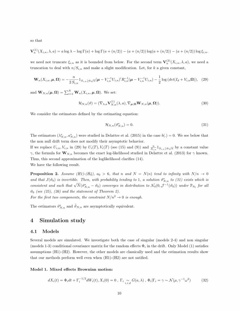
Several models are simulated. We investigate both the case of singular (models 2-4) and non singular(models 1-3) conditional covariance matrix for the random effects Φi in the drift. Only Model (1) satisfiesassumptions (H1)-(H2). However, the other models are classically used and the estimation results showthat our methods perform well even when (H1)-(H2) are not satified.

Model 1. Mixed effects Brownian motion:

dXi(t) = Φidt+ Γ−1/2i dWi(t), Xi(0) = 0 , Γi ∼

i.i.dG(a, λ) , Φi|Γi = γ ∼ N (µ, γ−1ω2) (32)

10

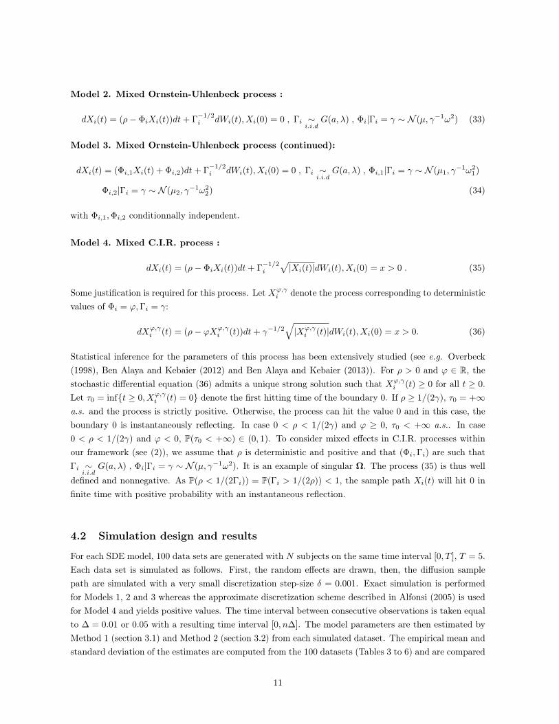
Model 2. Mixed Ornstein-Uhlenbeck process :

dXi(t) = (ρ− ΦiXi(t))dt+ Γ−1/2i dWi(t), Xi(0) = 0 , Γi ∼

i.i.dG(a, λ) , Φi|Γi = γ ∼ N (µ, γ−1ω2) (33)

Model 3. Mixed Ornstein-Uhlenbeck process (continued):

dXi(t) = (Φi,1Xi(t) + Φi,2)dt+ Γ−1/2i dWi(t), Xi(0) = 0 , Γi ∼

i.i.dG(a, λ) , Φi,1|Γi = γ ∼ N (µ1, γ

−1ω21)

Φi,2|Γi = γ ∼ N (µ2, γ−1ω2

2) (34)

with Φi,1,Φi,2 conditionnally independent.

Model 4. Mixed C.I.R. process :

dXi(t) = (ρ− ΦiXi(t))dt+ Γ−1/2i

√|Xi(t)|dWi(t), Xi(0) = x > 0 . (35)

Some justification is required for this process. Let Xϕ,γi denote the process corresponding to deterministic

values of Φi = ϕ,Γi = γ:

dXϕ,γi (t) = (ρ− ϕXϕ,γ

i (t))dt+ γ−1/2√|Xϕ,γ

i (t)|dWi(t), Xi(0) = x > 0. (36)

Statistical inference for the parameters of this process has been extensively studied (see e.g. Overbeck(1998), Ben Alaya and Kebaier (2012) and Ben Alaya and Kebaier (2013)). For ρ > 0 and ϕ ∈ R, thestochastic differential equation (36) admits a unique strong solution such that Xϕ,γ

i (t) ≥ 0 for all t ≥ 0.Let τ0 = inft ≥ 0, Xϕ,γ

i (t) = 0 denote the first hitting time of the boundary 0. If ρ ≥ 1/(2γ), τ0 = +∞a.s. and the process is strictly positive. Otherwise, the process can hit the value 0 and in this case, theboundary 0 is instantaneously reflecting. In case 0 < ρ < 1/(2γ) and ϕ ≥ 0, τ0 < +∞ a.s.. In case0 < ρ < 1/(2γ) and ϕ < 0, P(τ0 < +∞) ∈ (0, 1). To consider mixed effects in C.I.R. processes withinour framework (see (2)), we assume that ρ is deterministic and positive and that (Φi,Γi) are such thatΓi ∼

i.i.dG(a, λ) , Φi|Γi = γ ∼ N (µ, γ−1ω2). It is an example of singular Ω. The process (35) is thus well

defined and nonnegative. As P(ρ < 1/(2Γi)) = P(Γi > 1/(2ρ)) < 1, the sample path Xi(t) will hit 0 infinite time with positive probability with an instantaneous reflection.

4.2 Simulation design and results

For each SDE model, 100 data sets are generated with N subjects on the same time interval [0, T ], T = 5.Each data set is simulated as follows. First, the random effects are drawn, then, the diffusion samplepath are simulated with a very small discretization step-size δ = 0.001. Exact simulation is performedfor Models 1, 2 and 3 whereas the approximate discretization scheme described in Alfonsi (2005) is usedfor Model 4 and yields positive values. The time interval between consecutive observations is taken equalto ∆ = 0.01 or 0.05 with a resulting time interval [0, n∆]. The model parameters are then estimated byMethod 1 (section 3.1) and Method 2 (section 3.2) from each simulated dataset. The empirical mean andstandard deviation of the estimates are computed from the 100 datasets (Tables 3 to 6) and are compared

11

with those of the estimates based on a direct observation of the random effects (Tables 1 and 2). As theparameters of Gamma distributions are uneasy to estimate in practice, we use an other parametrizationin terms of m = a/λ and t = ψ(a) − log(λ), and we present the estimates of m and t rather than theestimates of a and λ.Both estimation procedures require some truncations. Let us make some remarks about the truncationused in the first estimation method. Although it performs well in theory, the truncation defined bymeans of the sets Fi,n is not adequate for a practical use. We have indeed observed that, even for verysmall values of α, a large number of simulated trajectories do not belong to the sets Fi,n (see (16)),leading to poor estimation performances. For implementing the first method, we have thus replaced1Fi,n by 1(Zi,n≥c/

√n) in the definition of Un(Xi,n, ϑ) and then numerically optimized the corresponding

new contrast. Here, we choose c = 0.1. The interest of introducing the sets Fi,n was that they do notdepend on the parameters and this simplifies differentiation. However, the main theoretical proof onlyrequires the condition Zi,n ≥ c/

√n) (see Lemma 2). The present simulation study shows that the method

performs well in practice. Concerning the second estimation method, we use k = 0.1 (see (29)).We observe from Tables 3 to 6 that the two estimation methods have similar performances overall. Bothestimate the parameters with very little bias whatever the model and the values of n and N . Thestandard deviations of the estimates are very close for the two methods as well, except in Model 4where the estimates are more variable with method 1 than with method 2. We guess that the numericaloptimisation of the first contrast is more difficult than the one of the second contrast which decouplesthe estimation of the parameters of the conditional Gaussian distribution from the estimation of theparameters of the Gamma distribution. We can remark that the estimates for m and t obtained from theobservations of the SDEs have similar standard deviations as those obtained from a direct observation ofthe random effects, whereas they are higher for parameters µ and Ω (except for Model 1 where they areequal). This is expected from the theory (see remark following Theorem 2). The bias and the standarddeviations of the estimates generally decrease as N increases. When N is fixed, increasing the numbern of observations per trajectory decreases bias but does not have any impact on the estimates standarddeviations. This is in accordance with the theory since the asymptotic distribution of the estimates isobtained when N/n→ 0 or N/n2 → 0 according to the parameters, and the rate of convergence is

√N .

Although n = 200 does not fulfill N/n → 0 in our simulation design, the results in this case are verysatisfactory which encourages the use of these two estimation methods not only for high but also moderatevalues of n. Let us stress that assumptions (H1)-(H2) are not satified by Models 2, 3 and 4. This doesnot deteriorate the performances of the estimation methods. Note also that although the matrix Ω issingular in Models 2 and 4, the model parameters are well estimated.

12

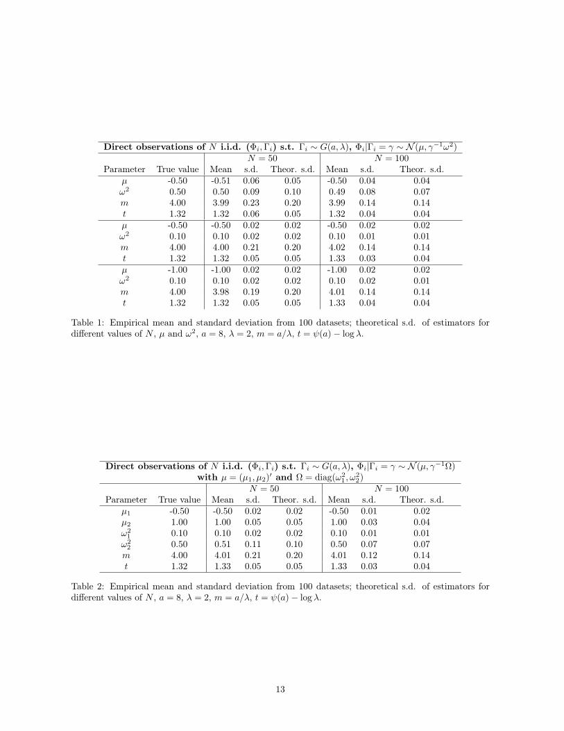
Direct observations of N i.i.d. (Φi,Γi) s.t. Γi ∼ G(a, λ), Φi|Γi = γ ∼ N (µ, γ−1ω2)N = 50 N = 100

Parameter True value Mean s.d. Theor. s.d. Mean s.d. Theor. s.d.µ -0.50 -0.51 0.06 0.05 -0.50 0.04 0.04ω2 0.50 0.50 0.09 0.10 0.49 0.08 0.07m 4.00 3.99 0.23 0.20 3.99 0.14 0.14t 1.32 1.32 0.06 0.05 1.32 0.04 0.04µ -0.50 -0.50 0.02 0.02 -0.50 0.02 0.02ω2 0.10 0.10 0.02 0.02 0.10 0.01 0.01m 4.00 4.00 0.21 0.20 4.02 0.14 0.14t 1.32 1.32 0.05 0.05 1.33 0.03 0.04µ -1.00 -1.00 0.02 0.02 -1.00 0.02 0.02ω2 0.10 0.10 0.02 0.02 0.10 0.02 0.01m 4.00 3.98 0.19 0.20 4.01 0.14 0.14t 1.32 1.32 0.05 0.05 1.33 0.04 0.04

Table 1: Empirical mean and standard deviation from 100 datasets; theoretical s.d. of estimators fordifferent values of N , µ and ω2, a = 8, λ = 2, m = a/λ, t = ψ(a)− log λ.

Direct observations of N i.i.d. (Φi,Γi) s.t. Γi ∼ G(a, λ), Φi|Γi = γ ∼ N (µ, γ−1Ω)with µ = (µ1, µ2)′ and Ω = diag(ω2

1 , ω22)

N = 50 N = 100Parameter True value Mean s.d. Theor. s.d. Mean s.d. Theor. s.d.

µ1 -0.50 -0.50 0.02 0.02 -0.50 0.01 0.02µ2 1.00 1.00 0.05 0.05 1.00 0.03 0.04ω2

1 0.10 0.10 0.02 0.02 0.10 0.01 0.01ω2

2 0.50 0.51 0.11 0.10 0.50 0.07 0.07m 4.00 4.01 0.21 0.20 4.01 0.12 0.14t 1.32 1.33 0.05 0.05 1.33 0.03 0.04

Table 2: Empirical mean and standard deviation from 100 datasets; theoretical s.d. of estimators fordifferent values of N , a = 8, λ = 2, m = a/λ, t = ψ(a)− log λ.

13

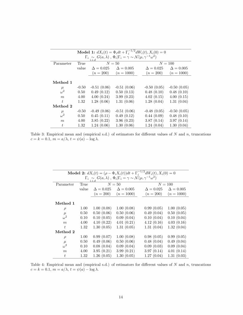
Model 1: dXi(t) = Φidt+ Γ−1/2i dWi(t), Xi(0) = 0

Γi ∼i.i.d

G(a, λ) , Φi|Γi = γ ∼ N (µ, γ−1ω2)

Parameter True N = 50 N = 100value ∆ = 0.025 ∆ = 0.005 ∆ = 0.025 ∆ = 0.005

(n = 200) (n = 1000) (n = 200) (n = 1000)

Method 1µ -0.50 -0.51 (0.06) -0.51 (0.06) -0.50 (0.05) -0.50 (0.05)ω2 0.50 0.49 (0.12) 0.50 (0.13) 0.48 (0.10) 0.48 (0.10)m 4.00 4.00 (0.24) 3.99 (0.23) 4.02 (0.15) 4.00 (0.15)t 1.32 1.28 (0.06) 1.31 (0.06) 1.28 (0.04) 1.31 (0.04)

Method 2µ -0.50 -0.49 (0.06) -0.51 (0.06) -0.48 (0.05) -0.50 (0.05)ω2 0.50 0.45 (0.11) 0.49 (0.12) 0.44 (0.09) 0.48 (0.10)m 4.00 3.85 (0.22) 3.96 (0.23) 3.87 (0.14) 3.97 (0.14)t 1.32 1.24 (0.06) 1.30 (0.06) 1.24 (0.04) 1.30 (0.04)

Table 3: Empirical mean and (empirical s.d.) of estimators for different values of N and n, truncationsc = k = 0.1, m = a/λ, t = ψ(a)− log λ.

Model 2: dXi(t) = (ρ− ΦiXi(t))dt+ Γ−1/2i dWi(t), Xi(0) = 0

Γi ∼i.i.d

G(a, λ) , Φi|Γi = γ ∼ N (µ, γ−1ω2)

Parameter True N = 50 N = 100value ∆ = 0.025 ∆ = 0.005 ∆ = 0.025 ∆ = 0.005

(n = 200) (n = 1000) (n = 200) (n = 1000)

Method 1ρ 1.00 1.00 (0.08) 1.00 (0.08) 0.99 (0.05) 1.00 (0.05)µ 0.50 0.50 (0.06) 0.50 (0.06) 0.49 (0.04) 0.50 (0.05)ω2 0.10 0.10 (0.05) 0.09 (0.04) 0.10 (0.04) 0.10 (0.04)m 4.00 4.10 (0.22) 4.01 (0.21) 4.12 (0.16) 4.03 (0.16)t 1.32 1.30 (0.05) 1.31 (0.05) 1.31 (0.04) 1.32 (0.04)

Method 2ρ 1.00 0.99 (0.07) 1.00 (0.08) 0.98 (0.05) 0.99 (0.05)µ 0.50 0.49 (0.06) 0.50 (0.06) 0.48 (0.04) 0.49 (0.04)ω2 0.10 0.08 (0.04) 0.09 (0.04) 0.09 (0.03) 0.09 (0.04)m 4.00 3.95 (0.21) 3.99 (0.21) 3.97 (0.14) 4.01 (0.14)t 1.32 1.26 (0.05) 1.30 (0.05) 1.27 (0.04) 1.31 (0.03)

Table 4: Empirical mean and (empirical s.d.) of estimators for different values of N and n, truncationsc = k = 0.1, m = a/λ, t = ψ(a)− log λ.

14

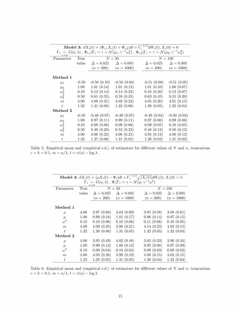
Model 3: dXi(t) = (Φi,1Xi(t) + Φi,2)dt+ Γ−1/2i dWi(t), Xi(0) = 0

Γi ∼i.i.d

G(a, λ) , Φi,1|Γi = γ ∼ N (µ1, γ−1ω2

1) , Φi,2|Γi = γ ∼ N (µ2, γ−1ω2

2)

Parameter True N = 50 N = 100value ∆ = 0.025 ∆ = 0.005 ∆ = 0.025 ∆ = 0.005

(n = 200) (n = 1000) (n = 200) (n = 1000)

Method 1µ1 -0.50 -0.50 (0.10) -0.50 (0.08) -0.51 (0.08) -0.51 (0.05)µ2 1.00 1.01 (0.14) 1.01 (0.13) 1.01 (0.10) 1.00 (0.07)ω2

1 0.10 0.13 (0.14) 0.14 (0.22) 0.16 (0.20) 0.12 (0.07)ω2

2 0.50 0.61 (0.35) 0.59 (0.35) 0.63 (0.45) 0.55 (0.20)m 4.00 4.09 (0.31) 4.02 (0.22) 4.05 (0.20) 4.01 (0.15)t 1.32 1.31 (0.08) 1.33 (0.06) 1.30 (0.05) 1.32 (0.04)

Method 2µ1 -0.50 -0.48 (0.07) -0.49 (0.07) -0.49 (0.04) -0.50 (0.04)µ2 1.00 0.97 (0.11) 0.99 (0.11) 0.97 (0.06) 0.99 (0.06)ω2

1 0.10 0.09 (0.06) 0.09 (0.06) 0.09 (0.05) 0.10 (0.05)ω2

2 0.50 0.49 (0.20) 0.52 (0.23) 0.48 (0.13) 0.50 (0.13)m 4.00 3.96 (0.22) 4.00 (0.21) 3.95 (0.12) 4.00 (0.12)t 1.32 1.27 (0.06) 1.31 (0.05) 1.26 (0.03) 1.31 (0.03)

Table 5: Empirical mean and (empirical s.d.) of estimators for different values of N and n, truncationsc = k = 0.1, m = a/λ, t = ψ(a)− log λ.

Model 4: dXi(t) = (ρXi(t)− Φi)dt+ Γ−1/2i

√|Xi(t)|dWi(t), Xi(0) = 5

Γi ∼i.i.d

G(a, λ) , Φi|Γi = γ ∼ N (µ, γ−1ω2)

Parameter True N = 50 N = 100value ∆ = 0.025 ∆ = 0.005 ∆ = 0.025 ∆ = 0.005

(n = 200) (n = 1000) (n = 200) (n = 1000)

Method 1ρ 4.00 3.97 (0.68) 4.04 (0.69) 3.85 (0.58) 3.88 (0.61)µ 1.00 0.99 (0.16) 1.01 (0.17) 0.96 (0.14) 0.97 (0.15)ω2 0.10 0.10 (0.06) 0.10 (0.06) 0.11 (0.06) 0.10 (0.05)m 4.00 4.09 (0.25) 3.98 (0.21) 4.14 (0.23) 4.02 (0.15)t 1.32 1.30 (0.06) 1.31 (0.05) 1.32 (0.05) 1.32 (0.04)

Method 2ρ 4.00 3.95 (0.49) 4.02 (0.48) 3.82 (0.33) 3.90 (0.34)µ 1.00 0.99 (0.12) 1.00 (0.12) 0.95 (0.08) 0.97 (0.09)ω2 0.10 0.09 (0.04) 0.10 (0.04) 0.09 (0.03) 0.09 (0.03)m 4.00 4.03 (0.20) 3.99 (0.19) 4.08 (0.15) 4.02 (0.15)t 1.32 1.28 (0.05) 1.31 (0.05) 1.30 (0.04) 1.32 (0.04)

Table 6: Empirical mean and (empirical s.d.) of estimators for different values of N and n, truncationsc = k = 0.1, m = a/λ, t = ψ(a)− log λ.

15

5 Implementation on real data

We now analyze some real neuronal data that are available in the R-package mixedsde. These data werefirst studied by Picchini et al. (2008, 2010). A complete description can be found in Dion (2016). Thedataset is composed of N = 240 membrane potential trajectories. The observations are expressed inVolts. Each trajectory is observed at n = 2000 equidistant time points on a common time interval [0, T ]

with T = 0.3s. Hence, the sampling time interval is ∆ = 0.00015s. Models of the form:

dXi(t) = (Φi,1 − Φi,2Xi(t))dt+ Ψiσ(Xi(t))dWi(t) , Xi(0) = xi, (37)

have been proposed for describing this kind of data. This formalism includes the Ornstein-Uhlenbeckmodel (OU): σ(x) = 1, and the Cox-Ingersoll-Ross model (CIR): σ(x) =

√|x|. Note that fixed ef-

fect Ornstein-Uhlenbeck diffusions are often used for neuronal data. The fixed effect CIR model wasinvestigated by Höpfner (2007).The parameters in (37) have a biological meaning: Φi,1 represents the local average input received by theneuron after the ith spike, and Φi,2 is the time constant of the neuron. The parameters Φi,1, Φi,2 andΨi can either be fixed or random but to our knowledge, only models with fixed effects in the diffusioncoefficient were used for describing the present dataset (see Picchini et al. (2008, 2010); Dion (2016); Dionet al. (2016)). Here, we try to answer two questions:

1) Which of the OU or the CIR is the most appropriate SDE for describing the data?

2) Which parameter should be fixed or random?

For that purpose, we estimate the OU in different configurations:

a. Φi,1 random s.t. Φi,1|Γi∼N (µ1, ω21/Γi), Φi,2 = µ2 fixed, Ψi = 1/

√Γi random, Γi∼G(a, λ), ,

b. Φi,1 = µ1 fixed, Φi,2 random s.t. Φi,2|Γi ∼ N (µ2, ω22/Γi), Ψi = 1/

√Γi random, Γi∼G(a, λ),

c. Φi,1 and Φi,2 random s.t. Φi,1|Γi∼N (µ1, ω21/Γi) and Φi,2|Γi∼N (µ2, ω

22/Γi), Φi,1,Φi,2 independent,

Ψi = 1/√

Γi random, Γi∼G(a, λ).

and the CIR in configuration b. (see remarks about the CIR in the simulation section).To allow the estimation of both CIR and OU, the two trajectories taking negative values are omitted,leading to N = 238. The observations take very small values (9 × 10−3 Volts on average). This cancause numerical difficulties such as lack of precision of the calculations. To avoid this, we change volts inmillivolts and seconds in milliseconds (T = 300 ms). Parameter estimation can be performed by meansof the methods described above. We favor the second method which is more stable numerically. We thenidentify the most appropriate model by comparing the BIC values. BIC is defined as −2 log L+ d log(N)

where L denotes the likelihood of the observations evaluated at the parameter estimate and d is thenumber of model parameters. Here, L is not explicit, thus approximated by the approximate likelihoodgiven by equations (13) and (14). The different BIC values and the parameter estimates are reportedin Table 5. Note that E(1/Γi) = λ/(a − 1) is a more relevant value in this model as it represents theexpectation of the square of the random effect Ψi. From the BIC criterion, the Cox-Ingersoll-Ross modelbetter suits to the data than Ornstein-Uhlenbeck models. To our knowledge, there does not exist any

16

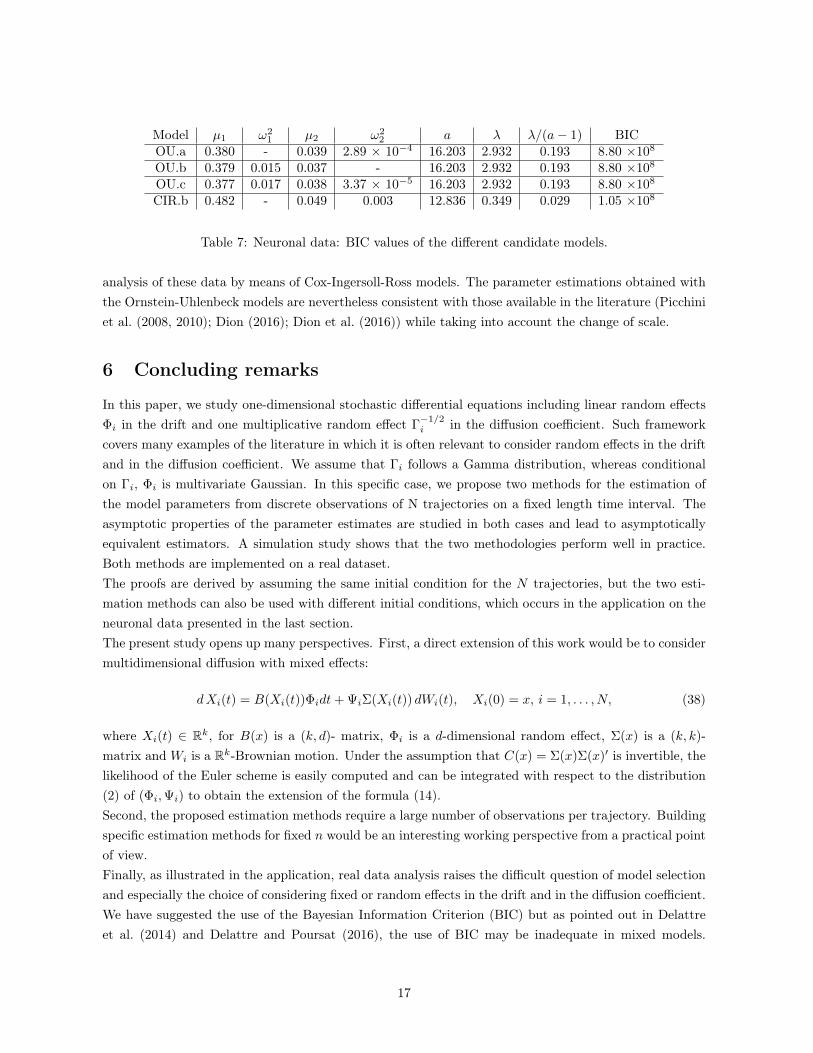
Model µ1 ω21 µ2 ω2

2 a λ λ/(a− 1) BICOU.a 0.380 - 0.039 2.89 × 10−4 16.203 2.932 0.193 8.80 ×108

OU.b 0.379 0.015 0.037 - 16.203 2.932 0.193 8.80 ×108

OU.c 0.377 0.017 0.038 3.37 × 10−5 16.203 2.932 0.193 8.80 ×108

CIR.b 0.482 - 0.049 0.003 12.836 0.349 0.029 1.05 ×108

Table 7: Neuronal data: BIC values of the different candidate models.

analysis of these data by means of Cox-Ingersoll-Ross models. The parameter estimations obtained withthe Ornstein-Uhlenbeck models are nevertheless consistent with those available in the literature (Picchiniet al. (2008, 2010); Dion (2016); Dion et al. (2016)) while taking into account the change of scale.

6 Concluding remarks

In this paper, we study one-dimensional stochastic differential equations including linear random effectsΦi in the drift and one multiplicative random effect Γ

−1/2i in the diffusion coefficient. Such framework

covers many examples of the literature in which it is often relevant to consider random effects in the driftand in the diffusion coefficient. We assume that Γi follows a Gamma distribution, whereas conditionalon Γi, Φi is multivariate Gaussian. In this specific case, we propose two methods for the estimation ofthe model parameters from discrete observations of N trajectories on a fixed length time interval. Theasymptotic properties of the parameter estimates are studied in both cases and lead to asymptoticallyequivalent estimators. A simulation study shows that the two methodologies perform well in practice.Both methods are implemented on a real dataset.The proofs are derived by assuming the same initial condition for the N trajectories, but the two esti-mation methods can also be used with different initial conditions, which occurs in the application on theneuronal data presented in the last section.The present study opens up many perspectives. First, a direct extension of this work would be to considermultidimensional diffusion with mixed effects:

dXi(t) = B(Xi(t))Φidt+ ΨiΣ(Xi(t)) dWi(t), Xi(0) = x, i = 1, . . . , N, (38)

where Xi(t) ∈ Rk, for B(x) is a (k, d)- matrix, Φi is a d-dimensional random effect, Σ(x) is a (k, k)-matrix and Wi is a Rk-Brownian motion. Under the assumption that C(x) = Σ(x)Σ(x)′ is invertible, thelikelihood of the Euler scheme is easily computed and can be integrated with respect to the distribution(2) of (Φi,Ψi) to obtain the extension of the formula (14).Second, the proposed estimation methods require a large number of observations per trajectory. Buildingspecific estimation methods for fixed n would be an interesting working perspective from a practical pointof view.Finally, as illustrated in the application, real data analysis raises the difficult question of model selectionand especially the choice of considering fixed or random effects in the drift and in the diffusion coefficient.We have suggested the use of the Bayesian Information Criterion (BIC) but as pointed out in Delattreet al. (2014) and Delattre and Poursat (2016), the use of BIC may be inadequate in mixed models.

17

Building statistical testing methods to decide which parameter is a challenging perspective.

References

Alfonsi, A. (2005). On the discretization schemes for the CIR (and Bessel squared) processes. MonteCarlo methods and Applications, 11:355–384.

Ben Alaya, M. and Kebaier, M. (2012). Parameter estimation for the square-root diffusions: Ergodic andnonergodic cases. Stochastic Models, 28:609–634.

Ben Alaya, M. and Kebaier, M. (2013). Asymptotic behavior of the maximum likelihood estimator forergodic and nonergodic square-root diffusions. Stochastic Analysis and Applications, 31:552–573.

Delattre, M., Genon-Catalot, V., and Larédo, C. (2016). Parametric inference for discrete observationsof diffusion with mixed effects in the drift or in the diffusion coefficient. preprint MAP5 2016-15.

Delattre, M., Genon-Catalot, V., and Samson, A. (2013). Maximum likelihood estimation for stochasticdifferential equations with random effects. Scandinavian Journal of Statistics, 40:322–343.

Delattre, M., Genon-Catalot, V., and Samson, A. (2015). Estimation of population parameters in stochas-tic differential equations with random effects in the diffusion coefficient. ESAIM Probability and Statis-tics, 19:671–688.

Delattre, M. and Lavielle, M. (2013). Coupling the saem algorithm and the extended kalman filter formaximum likelihood estimation in mixed-effects diffusion models. Statistics and its interface, 6(4):519–532.

Delattre, M. and Poursat, M. (2016). Bic strategies for model choice in a population approach. preprint.

Delattre, M., Poursat, M., and Lavielle, M. (2014). A note on BIC in mixed-effects models. ElectronicJournal of Statistics, 8:456–475.

Dion, C. (2016). Nonparametric estimation in a mixed-effect ornstein-uhlenbeck model. Metrika.

Dion, C., Hermann, S., and Samson, A. (2016). Mixedsde : a r package to fit mixed stochastic differentialequations. Preprint hal-01305574 https://hal.archives-ouvertes.fr/hal-01305574.

Ditlevsen, S. and De Gaetano, A. (2005). Mixed effects in stochastic differential equation models. REV-STAT Statistical Journal, 3:137–153.

Donnet, S. and Samson, A. (2008). Parametric inference for mixed models defined by stochastic differentialequations. ESAIM P&S, 12:196–218.

Forman, J. and Picchini, U. (2016). Stochastic differential equation mixed effects models for tumor growthand response to treatment. preprint.

Höpfner, R. (2007). On a set of data for the membrane potential in a neuron. Math. Biosci., 207(2):275–301.

18

Leander, J., Almquist, J., Ahlstrom, C., Gabrielsson, J., and Jirstrand, M. (2015). Mixed effects modelingusing stochastic differential equations: Illustrated by pharmacokinetic data of nicotinic acid in obesezucker rats. AAPS Journal, DOI: 10.1208/s12248-015-9718-8.

Overbeck, L. (1998). Estimation for continuous branching processes. Scandinavian Journal of Statistics,25:111–126.

Picchini, U., De Gaetano, A., and Ditlevsen, S. (2010). Stochastic differential mixed-effects models.Scand. J. Statist., 37:67–90.

Picchini, U. and Ditlevsen, S. (2011). Practicle estimation of high dimensional stochastic differentialmixed-effects models. Computational Statistics & Data Analysis, 55:1426–1444.

Picchini, U., Ditlevsen, S., and De Gaetano, A. (2008). Parameters of the diffusion leaky integrate-and-fireneuronal model for slowly fluctuating signal. Neural Computation, 20:2696–2714.

Pinheiro, J. and Bates, D. (2000). Mixed-effect models in S and Splus. Springer-Verlag.

The corresponding author is:Catherine Larédo (catherine.laredo@jouy.inra.fr )Laboratoire MaIAGE, I.N.R.A., Jouy-en-Josas, France.

7 Appendix

7.1 Proof of Proposition 1

Assume first that Ω is invertible. Integrating (5) with respect to the distribution N (µ, γ−1Ω) yields theexpression:

Λn(Xi,n, γ,µ,Ω) = γn/2 exp (−γ2Si,n)

γd/2

(2π)d/2(det(Ω))1/2×∫

Rd

exp (γ(ϕ′Ui,n −1

2ϕ′Vi,nϕ)) exp (−γ

2(ϕ− µ)′Ω−1(ϕ− µ))dϕ

= γn/2 exp (−γ2Si,n)

(det(Σi,n)

det(Ω)

)1/2

exp (−γ2Ti,n(µ,Ω))

whereTi,n(µ,Ω) = µ′Ω−1µ−m′i,nΣ−1

i,nmi,n, (39)

andΣi,n = Ω(Id + Vi,nΩ)−1, mi,n = Σi,n(Ui,n + Ω−1µ).

Computations using matrices equalities and (7),(8), (10) yield that Ti,n(µ,Ω) is equal to the expressiongiven in (11), i.e.:

Ti,n(µ,Ω) = (µ− V −1i,n Ui,n)′R−1

i,n(µ− V −1i,n Ui,n)− U ′i,nV −1

i,n Ui,n.

19

Noting that det(Σi,n)det(Ω) = (det(Id + Vi,nΩ))−1, we get

Λn(Xi,n, γ,µ,Ω) = γn/2(det(Id + Vi,nΩ))−1/2 exp[−γ

2(Si,n + Ti,n(µ,Ω))

].

We multiply Λn(Xi,n, γ,µ,Ω) by the Gamma density (λa/Γ(a))γa−1 exp (−λγ) and, on the set Ei,n(ϑ)

(see (12)), we can integrate w.r.t. to γ on (0,+∞). This gives Ln(Xi,n, ϑ).At this point, we observe that the formula (14) and the set Ei,n(ϑ) are still well defined for non invertibleΩ. Consequently, we can consider Ln(Xi,n, ϑ) as an approximate likelihood for non invertible Ω.

We now consider the set FN,n introduced in (16) which is defined under (H4). Let us stress that this setdoes not depend on unknown parameters.

7.2 Proof of Lemma 1

By (10)-(11), we have, using µ− V −1i,n Ui,n = V −1

i,n (Vi,nµ− Ui,n),

Ti,n(µ,Ω) = µ′Vi,n(Id+ΩVi,n)−1µ+U ′i,n[(Id + ΩVi,n)−1 − Id

]V −1i,n Ui,n−2µ′Vi,n(Id+ΩVi,n)−1V −1

i,n Ui,n.

For two nonnegative symmetric matrices A,B, we have A ≤ B if and only if for all vector x, x′Ax ≤ x′Bxand in this case, for all vectors x, y, 2x′Ay ≤ (x+ y)′B(x+ y). We write:

(Id + ΩVi,n)−1 − Id = (Id + ΩVi,n)−1 [Id − (Id + ΩVi,n)] = −(Id + ΩVi,n)−1ΩVi,n ≤ 0.

Therefore, using (H4) and the previous inequality with A = Vi,n(Id + ΩVi,n)−1V −1i,n , B = Id yields

U ′i,n[(Id + ΩVi,n)−1 − Id

]V −1i,n Ui,n = −U ′i,n(Id + ΩVi,n)−1ΩUi,n ≥ −U ′i,nΩUi,n ≥ −c1‖Ui,n‖2,

−2µ′Vi,n(Id + ΩVi,n)−1V −1i,n Ui,n ≥ −(µ+ Ui,n)′(µ+ Ui,n) ≥ −2(‖Ui,n‖2 +m2).

This yieldsTi,n(µ,Ω) ≥ −

[(c1 + 2)‖Ui,n‖2 + 2m2

].

We consider (see (12)-(16)): Mi,n = maxc1 + 2, 2m2(‖Ui,n‖2 + 1), and for α > 0, the set Fi,n =

1n (Si,n −Mi,n) ≥ α√

n. Then, for all ϑ, we have Fi,n ⊂ Ei,n(ϑ).

For simplicity of notations, we continue the proof for d = 1.Fix a value ϑ0. We study the probability of Fi,n and FN,n under Pϑ0 . For all fixed i = 1, . . . , N , as ntends to infinity, Ui,n tends to Ui(T ) and Vi,n tends to Vi(T ). Hence, Mi,n/n tends to 0 in probability.Moreover, 1

nSi,n tends to Γ−1i . Thus, Pϑ0(Fi,n) tends to 1 as n tends to infinity. This is not enough

for our purpose because we have to deal with the N trajectories simultaneously. Thus, we look for acondition on N,n ensuring that Pϑ0(FN,n) →N,n→+∞ 1. As Pϑ0(∪Ni=1F

ci,n) ≤ NPθ0(F c1,n), we will find a

condition ensuring that NPϑ0(F c1,n) tends to 0. More precisely, we prove that, if a0 > 4,

Pϑ0(F c1,n) .

1

n2(40)

20

which explains the constraint N/n2 → 0.Let us study the set F c1,n = 1

n (S1,n −M1,n) ≤ α√n. For the rest of the proof, as we consider only the

process X1 and let n tend to infinity, we set X1 = X, Ψ1 = Ψ,Γ1 = Γ = Ψ−2,Φ1 = Φ, S1,n = Sn(X),M1,n = Mn(X), U1,n = Un(X), V1,n = Vn(X). We split successively by Mn(X)/n > α/

√n and by

Ψ2 < 4α/√n and obtain:

Pϑ0(

1

n(Sn(X)−Mn(X)) ≤ α√

n) ≤ Pϑ0

(Mn(X)

n>

α√n

) + Pϑ0(Sn(X)

n≤ 2 α√

n)

≤ Pϑ0(Mn(X)

n>

α√n

) + Pϑ0(Ψ2 <

4α√n

) + Pϑ0(Ψ2 − Sn(X)

n≥ 1

2Ψ2).

The last part is obtained as follows. Note that (Ψ2 ≥ 4 α√n

) = (Ψ2 − 2 α√n≥ Ψ2

2 ). Therefore,

(Sn(X)

n≤ 2 α√

n,Ψ2 ≥ 4 α√

n)) = (Ψ2 − Sn(X)

n≥ Ψ2 − 2 α√

n,Ψ2 ≥ 4 α√

n)) ⊂ (Ψ2 − Sn(X)

n≥ 1

2Ψ2).

We study successively the rates of convergence to 0 of the three terms of the bound of Pϑ0( 1n (Sn(X) −

Mn(X) ≤ α√n

). Using the Markov inequality for the middle term,

Pϑ0(Ψ2 <

4α√n

) = Pϑ0(Γ >

√n

4α) ≤ (

4α√n

)4Eϑ0Γ4 . n−2.

For the first term, we now check that, if Eϑ0Γ−4 < +∞, i.e. a0 > 4,

Pϑ0(Mn(X) ≥ α

√n) . n−2. (41)

For this, we have to study Eϑ0(Un(X)8|Φ,Ψ) (see (16)). We write Un(X) = U

(1)n + U

(2)n , where

U (1)n = Φ

n∑j=1

b(X(tj−1))

σ2(X(tj−1))

∫ tj

tj−1

b(X(s))ds, |U (1)n | ≤ |Φ|

K2

σ20

T.

Therefore, Eϑ0(U

(1)n )8|Φ,Ψ) . Φ8. Next,

U (2)n =

∫ T

0

Jns dWs, Jns = Ψ

n∑j=1

1(tj−1,tj ](s)b(X(tj−1))

σ2(X(tj−1))σ(X(s)).

For s ∈ [0, T ], |Jns | ≤ ΨK2/σ20 . This yields, by the B-D-G inequality, Eϑ0(((U

(2)n )8|Φ,Ψ) ≤ CK16σ−16

0 Ψ8T 4.

Now, Eϑ0Φ8 . µ8 + ω8Eϑ0Γ−4 and Eϑ0Ψ8 = Eϑ0Γ−4. Hence (41).It remains to study Pϑ0(Ψ2 − Sn(X)

n ≥ 12Ψ2) which is the most difficult term.

Lemma 3. Under (H1)-(H2), if a0 > 2,

Pϑ0(Ψ2 − Sn(X)

n≥ 1

2Ψ2) . n−2.

21

Proof of Lemma 3. We use the following classical development (see Comte et al. 2007, p.522):

(X((j + 1)∆))−X(j∆))2

∆= Ψ2σ2(X(j∆)) + Ψ2V

(1)j∆ (X) + 2Ψ3V

(2)j∆ (X)

+ 2ΦΨV(3)j∆ (X) +Rj∆(Φ,Ψ, X),

where

V(1)j∆ (X) =

1

∆

(∫ (j+1)∆

j∆

σ(X(s))dW (s)

)2

−∫ (j+1)∆

j∆

σ2(X(s))ds

(42)

V(2)j∆ (X) =

1

∆

∫ (j+1)∆

j∆

((j + 1)∆− u)σ′(X(u))σ2(X(u)dW (u) (43)

V(3)j∆ (X) = b(X(j∆))

∫ (j+1)∆

j∆

σ(X(s))dW (s) (44)

Rj∆(Φ,Ψ, X) =Φ2

∆

(∫ (j+1)∆

j∆

b(X(s))ds

)2

(45)

+2ΦΨ

∆

∫ (j+1)∆

j∆

(b(X(s)− b(X(j∆)))ds

∫ (j+1)∆

j∆

σ(X(s))dW (s)

+1

∆

∫ (j+1)∆

j∆

((j + 1)∆− u)KΦ,Ψ(X(u))du

where KΦ,Ψ(.)) = Ψ2[Φ2bσσ′ + Ψ2σ2(σ2)′′]. Therefore,

Sn(X)

n= Ψ2 + ν(1)

n + ν(2)n + ν(3)

n + ν(4)n . (46)

And

Pϑ0(Ψ2 − Sn(X)

n≥ 1

2Ψ2|Φ,Ψ) ≤

4∑i=1

Pϑ0(−ν(i)

n ≥Ψ2

8|Φ,Ψ)

For the term containing ν(1)n , we apply Lemma 3 of Comte et al. (2007, p.536) which states that, for

a continous process X adapted to (Ft), when the function σ(x) is upper bounded by K and for t(x) acontinous function:

P(

n∑j=1

t(X(j∆))V(1)j∆ (X) ≥ nε, ‖t‖2n ≤ v2) ≤ exp [−Cn ε2/2

2K4v2 + ε‖t‖∞K2v]

where C is a universal constant and ‖t‖2n = n−1∑nj=1 t

2(X(j∆)).We apply this result conditoning on Φ = ϕ, Ψ = ψ with t(x) = −1/σ2(x), v2 = σ−4

0 , ‖t‖∞ = σ−20 . Noting

that

−ν(1)n = Ψ2 1

n

n−1∑j=0

−1

σ2(X(j∆))V

(1)j∆ (X), (47)

22

we choose ε = 1/8 and simplifying by Ψ2, this yields

Pϑ0(−ν(1)n ≥ Ψ2/8|Φ = ϕ,Ψ = ψ) ≤ exp

(−Cn 1/(2× 82)

2K4σ−40 + (1/8)σ−4

0 K2

).

The upper bound is deterministic so Pϑ0(−ν(1)n ≥ Ψ2/8) ≤ exp (−cn), where c depends on K and σ0.

Next, we study ν(2)n :

−ν(2)n =

Ψ3

n

∫ n∆

0

Hn(s)dW (s), with (48)

Hn(s) = −n−1∑j=0

((j + 1)∆− s)σ′(X(s))σ2(X(s))

∆σ2(X(j∆))1(j∆,(j+1)∆](s), |Hn(s)| ≤ LK2

σ20

.

Hence,

Pϑ0(−ν(2)

n ≥ Ψ2/8|Φ = ϕ,Ψ = ψ)) = Pθ0(

∫ n∆

0

Hn(s)dW (s) ≥ n/(8Ψ)| Φ = ϕ,Ψ = ψ)

≤(

8Ψ

n

)2

Eθ0(

∫ n∆

0

H2n(s)ds|Φ = ϕ,Ψ = ψ) ≤

(8Ψ

n

LK2

σ20

)2

T.

Therefore, provided that Eϑ0Γ−1 < +∞, i.e. a0 > 1, Pϑ0(−ν(2)n ≥ Ψ2/8) . n−2.

Next, we study

−ν(3)n =

Ψ

n

∫ n∆

0

Kn(s)dW (s) with (49)

Kn(s) = −n−1∑j=0

1(j∆,(j+1)∆](s)2Φb(X(j∆))σ(X(s))

σ2(X(j∆)), |Kn(s)| ≤ 2|Φ|K

2

σ20

.

Thus,

Pϑ0(−ν(3)n ≥ Ψ2/8|Φ = ϕ,Ψ = ψ)) = Pϑ0(

∫ n∆

0

Kn(s)dW (s) ≥ nΨ/8|Φ = ϕ,Ψ = ψ)

≤(

8

nψ

)2

× 4ϕ2T (K2

σ20

)2

We have Eϑ0(Ψ−2Φ2) = Eϑ0(µ√

Γ+ωε)2 ≤ 2(µ2Eϑ0Γ+ω2) < +∞. Therefore, Pϑ0(−ν(3)n ≥ Ψ2/8) . n−2.

There remains to study:

ν(4)n =

1

n

n−1∑j=0

Rj∆(Φ,Ψ, X)

σ2(X(j∆)). (50)

We have:

Pϑ0(−ν(4)

n ≥ Ψ2/8|Φ = ϕ,Ψ = ψ) ≤ 82

ψ4Eϑ0

(ν(4)n )2||Φ = ϕ,Ψ = ψ)

.82

ψ4Eϑ0R

2j∆(Φ,Ψ, X)|Φ = ϕ,Ψ = ψ),

23

where (see (45)) R2j∆(Φ,Ψ, X) . ∆2

(Φ4 + (ΦΨ2 + Ψ4)2

)+ ∆−24Φ2Ψ2I2

j and

Ij =

∫ (j+1)∆

j∆

(b(X(s)− b(X(j∆)))ds

∫ (j+1)∆

j∆

σ(X(s))dW (s) (51)

Using Lemma 5 below, we find Eϑ0(I2j |Φ = ϕ,Ψ = ψ) . ∆4(ϕ2 + ψ2). Finally,

82

ψ4Eϑ0

R2j∆(Φ,Ψ, X)|Φ = ϕ,Ψ = ψ) . ∆2

(ψ−4ϕ4 + ψ4 + ϕ2 + ψ−2ϕ4)

). (52)

Therefore, we have Eϑ082Ψ−44R2

j∆(Φ,Ψ, X) . ∆2 if Eϑ0(Ψ−4Φ4 + Ψ4 + Φ2 + Ψ−2Φ4) < +∞ i.e.

Eϑ0(Γ−2) < +∞ which holds for a0 > 2.

This ends the proof of Lemma 3. The proof of Lemma 1 is now complete.

7.3 Proof of Theorem 1

Proof of Lemma 2Recall that we consider d = 1 (univariate effect in the drift). For simplicity of notations, we omit theindex n but keep the index i for the i-th sample path. We have (see (19 and (22)):

Zi −S

(1)i

n=

n

2a+ n(Sin− S

(1)i

n)− 2a

2a+ n

S(1)i

n+

2λ+ Ti(µ, ω2)

2a+ n.

Note that, using (11):

Ti(µ, ω2) =

Vi(1 + ω2Vi)

(µ− Ui

Vi

)2

− U2i

Vi=

U2i

(1 + ω2Vi)(µ2 − ω2)− 2µ

Ui(1 + ω2Vi)

, (53)

By the Hölder inequality, we obtain using (8) and (53):∣∣∣∣∣Zi − S(1)i

n

∣∣∣∣∣p

.

∣∣∣∣∣Sin − S(1)i

n

∣∣∣∣∣p

+ n−p

[1 + Ψ2p

i

(C

(1)i

n

)p+ U2p

i

].

Now, we apply Lemmas 8 and 6 of Section 8.2 and (64) of Section 8.1 and this yields the first inequality.For the second inequality, we write:

Z−1i −

n

S(1)i

=

(n

S(1)i

)2

Z−1i

(S

(1)i

n− Zi

)2

+

(n

S(1)i

)2(S

(1)i

n− Zi

).

On Fi, Zi ≥ c/√n, so:

∣∣∣∣∣Z−1i −

n

S(1)i

∣∣∣∣∣ 1Fi .

(n

C(1)i

)2

Ψ−4i

√n(S(1)i

n− Zi

)2

+

∣∣∣∣∣S(1)i

n− Zi

∣∣∣∣∣ .

24

Consequently,∣∣∣∣∣Z−1i −

n

S(1)i

∣∣∣∣∣p

1Fi.

(n

C(1)i

)2p

Ψ−4pi

np/2(S(1)i

n− Zi

)2p

+

∣∣∣∣∣S(1)i

n− Zi

∣∣∣∣∣p . (54)

Now, we take conditional expectation w.r.t. Ψi = ψ,Φi = ϕ and apply the Cauchy-Schwarz inequality.We use that, for n large enough, (see (64) of Section 8.1):

Eϑ(

(n

C(1)i

)4p

|Ψi = ψ,Φi = ϕ) = E

(n

C(1)i

)4p

= O(1).

And, we apply the first inequality to get the result. Now, we start proving Theorem 1. Omitting the index n in Ai,n, Bi,n, we have (see (20), (23), (24))

N−1/2 ∂UN,n

∂λ(ϑ) = N−1/2

N∑i=1

(aλ− Γi

)+R1,

N−1/2 ∂UN,n

∂a(ϑ) = N−1/2

N∑i=1

(−ψ(a) + log λ+ log Γi) +R2 +R′2,

N−1/2 ∂UN,n

∂µϑ) = N−1/2

N∑i=1

ΓiAi +R3 = N−1/2N∑i=1

ΓiAi(T ;µ, ω2) +R′3 +R3

N−1/2 ∂UN,n

∂ω2ϑ) = N−1/2 1

2

N∑i=1

(ΓiA

2i −Bi

)+R4

= N−1/2 1

2

N∑i=1

(ΓiA2i (T ;µ, ω2)−Bi(T, ω2)) +R′4 +R4.

The remainder terms are:

R1 = N−1/2N∑i=1

(Γi − Z−1i 1Fi), R2 = N−1/2

N∑i=1

(logZ−1i 1Fi − log Γi),

R′2 = N1/2(ψ(a+ (n/2))− log (a+ (n/2))) +N−1/2N∑i=1

1F ci,

R3 = N−1/2N∑i=1

Ai(Z−1i 1Fi − Γi), R4 = N−1/2 1

2

N∑i=1

A2i (Z−1i 1Fi − Γi),

R′3 = N−1/2N∑i=1

Γi(Ai −Ai(T ;µ, ω2)),

R′4 = N−1/2 1

2

N∑i=1

(Bi −Bi(T, ω2))− Γi(A2i −A2

i (T ;µ, ω2))).

The most difficult remainder terms are R1, R2, R3, R4. They are treated in Lemma 4 below. For the termR′2, we use that (ψ(a+ (n/2))− log (a+ (n/2))) = 0(n−1) (see (63)) and that, for a > 4, Pθ(F ci ) . n−2

(see (40)) to get that R′2 = OP (√N/n).

25

Using Lemma 6 in Section 8.2, it is easy to check that R′3 and R′4 are OP (√N/n).

Therefore, there remains to find the limiting distribution of:N−1/2

∑Ni=1

(aλ − Γi

),

N−1/2∑Ni=1 (−ψ(a) + log λ+ log Γi) ,

N−1/2∑Ni=1 ΓiAi(T ;µ, ω2),

N−1/2 12

∑Ni=1(Bi(T, ω

2)− ΓiA2i (T ;µ, ω2))

.

The first two components are exactly the score function corresponding to the exact observation of (Γi, i =

1, . . . , N) (see section 8.3). Hence, the first part of Theorem 1 is proved.The whole vector is ruled by the standard central limit theorem. To compute the limiting distribution, weuse results from Delattre et al. (2013) which deals with the case of Γi = γ fixed and Φi ∼ N (µ, γ−1ω2).It is proved in this paper that

Eϑ(Ai(T ;µ, ω2)|Γi = γ) = 0, Eϑ(Bi(T, ω2)− ΓiA

2i (T ;µ, ω2))|Γi = γ) = 0.

Hence, the third and fourth component are centered and the covariances between the first two componentsand the last two ones are null. Moreover, it is also proved that

Eϑ(A2i (T ;µ, ω2)|Γi = γ) = Bi(T ;ω2),

Eϑ(

1

2(γA2

i (T ;µ, ω2)−Bi(T ;ω2)

)2

|Γi = γ) =1

2Eϑ(2γA2

i (T ;µ, ω2)Bi(T ;ω2)−B2i (T ;ω2))|Γi = γ)

EϑAi(T ;µ, ω2)(γA2i (T ;µ, ω2)−Bi(T ;ω2))|Γi = γ) = EϑAi(T ;µ, ω2)(Bi(T, ω

2)|Γi = γ)

Hence, the covariance matrix of the last two components is equal to J(ϑ) defined in (25).The proof of the last item relies on the same tools with more cumbersome computations but no additionaldifficulty. Note that this part only requires that N,n both tend to infinity without further constraint. Sothe proof is complete.

Lemma 4. Recall (19). Then, for a > 4, (see (16) for the definition of Fi,n), R1, R2 are OP (√Nn ),

R3, R4 are OP (√

Nn ).

Proof. The proof goes in several steps. We have introduced

S(1)i = Ψ2

i

1

∆

n∑j=1

(Wi(tj)−Wi(tj−1)))2

= Γ−1i C

(1)i .

We know the exact distribution of S(1)i : C(1)

i is independent of Γi and has distribution χ2(n) = G(n/2, 1/2).By exact computations, using Gamma distributions (see Section 8)), we obtain:

Eϑ

(n

C(1)i

− 1

)= 1 +

2

n− 2, Eϑ

(n

C(1)i

− 1

)2

=2n+ 8

(n− 2)(n− 4)= O(n−1),

Eϑ logC(1)i /2− log (n/2) = ψ(n/2)− log (n/2) = O(n−1),Varϑ(logC

(1)i /2) = ψ′(n/2) = O(n−1).

26

Thus,1√N

N∑i=1

(n

S(1)i

− Γi

)= OP (

√N

n),

1√N

N∑i=1

(log

n

S(1)i

− log Γi

)= OP (

√N

n). (55)

Then, we have to study

1√N

N∑i=1

(Z−1i 1Fi

− n

S(1)i

),

1√N

N∑i=1

(log (Z−1

i )1Fi− log

n

S(1)i

). (56)

We write: (Z−1i 1Fi

− n

S(1)i

)=

(Z−1i −

n

S(1)i

)1Fi− n

S(1)i

1F ci.

For a > 4, Pϑ(F ci ) . n−2 (see (40)). This implies, after developping and applying the Cauchy-Schwarzinequality, noting that Γi = Ψ−2

i has moments of any order,

Eϑ

(1√N

N∑i=1

n

S(1)i

1F ci

)2

= O(N

n2), for a > 4. (57)

Next, apply Lemma 2,

Eϑ

∣∣∣∣∣ 1√N

N∑i=1

(Z−1i −

n

S(1)i

)1Fi

∣∣∣∣∣ .√N

nEϑ(1 + (1 + Φ2

i )(Ψ−2i + Ψ−4

i ) + Φ4i + Ψ4

i + Φ4iΨ−4i

).

As noted above, Ψi = Γ−1/2i , Eϑ(Ψ−qi ) < +∞ for all q ≥ 0. We can write Φi = µ + ωΨiεi with εi a

standard Gaussian variable independent of Ψi. We have

EϑΦ2iΨ−2i = Eϑ(µΨ−1

i + ωεi)2 < +∞, EϑΦ2

iΨ−4i = Eϑ(µΨ−2

i + ωΨ−1i εi)

2 < +∞, and for a > 2,

EϑΦ4i . 1 + EϑΨ4

i = 1 + EϑΓ−2i < +∞.

Thus, for a > 4,1√N

N∑i=1

(Z−1i 1Fi −

n

S(1)i

)= OP (

√N

n). (58)

Joining (55)(left)-(56)(left)-(57)-(58), we obtain that, for a > 4, R1 = OP (√Nn ).

Analogously, (log (Z−1

i )1Fi − logn

S(1)i

)=

(log (Z−1

i )− logn

S(1)i

)1Fi − 1F c

ilog

n

S(1)i

.

As above, we have

Eϑ

(1√N

N∑i=1

logn

S(1)i

1F ci

)2

= O(N

n2), for a > 4. (59)

27

And:

log (Z−1i )− log

n

S(1)i

= logS

(1)i

n− logZi

= (S

(1)i

n− Zi)

∫ 1

0

ds

1

sS

(1)i

n + (1− s)Zi− 1

S(1)i

n

+1

S(1)i

n

=

1

S(1)i

n

(S

(1)i

n− Zi) +

1

S(1)i

n

(S

(1)i

n− Zi)2

∫ 1

0

ds(1− s)

sS

(1)i

n + (1− s)Zi.

On Fi, ∣∣∣∣∣log (Z−1i )− log

n

S(1)i

∣∣∣∣∣ . 1

C(1)i

n

Ψ−2i

(∣∣∣∣∣S(1)i

n− Zi

∣∣∣∣∣+√n(S

(1)i

n− Zi)2

). (60)

Now, we take conditional expectation w.r.t. Φi = ϕ,Ψi = ψ, and apply first the Cauchy-Schwarzinequality and then Lemma 2. This yields:

Eϑ

(∣∣∣∣∣log (Z−1i )− log

n

S(1)i

∣∣∣∣∣ |Φi = ϕ,Ψi = ψ

).

1

n(1 + ψ−2(1 + ϕ2) + ψ2(1 + ϕ4) + ϕ2 + ϕ4 + ψ6). (61)

We have to check that the expectation above is finite. The worst term is EϑΨ6i = EϑΓ−3

i which requiresthe constraint a > 3. Thus, for a > 3, we have:

Eϑ1√N

∣∣∣∣∣N∑i=1

(log (Z−1i )− log

n

S(1)i

)1Fi

∣∣∣∣∣ = O(

√N

n).

Therefore, we have proved that R1, R2 are OP (√N/n).

For R3, R4, we proceed analogously but we have to deal with the terms Ai, A2i . We write again:

Z−1i 1Fi

− Γi = (Z−1i −

n

S(1)i

)1Fi− n

S(1)i

1F ci

+n

S(1)i

− Γi.

Using Lemma 6 and 7, we obtain:

Eϑ

∣∣∣∣∣ 1√N|N∑i=1

Ai(n

S(1)i

− Γi)

∣∣∣∣∣ .√N

nEϑ(Γi + Γ

1/2i ) = O(

√N

n),

Eϑ

∣∣∣∣∣ 1√N

N∑i=1

Ain

S(1)i

1F ci

∣∣∣∣∣ .√N

nEϑ(Γi + Γ

1/2i ) = O(

√N

n).

Applying now Lemma 2, we obtain:

Eϑ

∣∣∣∣∣ 1√N

N∑i=1

Ai(Z−1i −

n

S(1)i

)1Fi

∣∣∣∣∣ .√N

nEϑ(|Φi|(1 + Ψi + Ψ2

i ) + Φ2iΨi + Ψi + Ψ2

i + Ψ3i ).

28

This requires the constraint EϑΨ3i = EϑΓ

−3/2i < +∞, i.e. a > 3/2.

We proceed analogously for R4 and find that R4 = OP (√N/n) for a > 2.

The second order derivatives of −N−1UN,n(ϑ) are as follows. First, the derivatives corresponding to(λ, a):

− 1

N

∂2

∂λ2UN,n(ϑ) =

a

λ2− 1

N(a+ (n/2))

N∑i=1

Z−2i 1Fi

,

− 1

N

∂2

∂λ∂aUN,n(ϑ) = − 1

λ+

1

N(a+ (n/2))

N∑i=1

Z−1i 1Fi

,

− 1

N

∂2

∂a2UN,n(ϑ) = ψ′(a)− ψ′(a+ n/2) +

1

N(a+ n/2))

N∑i=1

1F ci.

Then, the cross derivatives w.r.t. (λ, a), (µ, ω2):

− 1

N

∂2

∂λ∂µUN,n(ϑ) =

1

N(a+ (n/2))

N∑i=1

1FiZ−2i Ai,

− 1

N

∂2

∂λ∂ω2UN,n(ϑ) =

1

2N(a+ (n/2))

N∑i=1

1FiZ−2i A2

i ,

− 1

N

∂2

∂a∂µUN,n(ϑ) = − 1

N(a+ (n/2))

N∑i=1

1FiZ−1i Ai,

− ∂2

∂a∂ω2UN,n(ϑ) = − 1

2N(a+ (n/2))

N∑i=1

1FiZ−1i A2

i .

Then, the derivatives corresponding to (µ, ω2):

− 1

N

∂2

∂µ2UN,n(ϑ) =

1

N

N∑i=1

1FiZ−1i Bi −

1

N(a+ (n/2))

N∑i=1

1FiZ−2i A2

i ,

− 1

N

∂2

∂µ∂ω2UN,n(ϑ) =

1

N

N∑i=1

1FiZ−1i AiBi −

1

N(a+ (n/2))

N∑i=1

1FiZ−2i A3

i ,

− 1

N

N∑i=1

1∂2

∂ω2∂ω2UN,n(ϑ) =

1

2N

N∑i=1

(1Fi2Z

−1i A2

iBi −B2i

)− 1

4N(a+ (n/2))

N∑i=1

1FiZ−2i A4

i .

By applying Lemmas 7 and 2, we can prove that the terms of the form N−1∑Ni=1 1FiZ

−αi Aβi B

δi converge,

as N,n tend to infinity, to EϑΓα1Aβ1 (T ;µ, ω2)Bδ1(T ;ω2). This implies that all terms of the form N−1(a+

(n/2))−1∑Ni=1 1FiZ

−αi Aβi B

δi converge to 0. So, all cross derivatives tend to 0 and the rest of derivatives

gives the limit J (ϑ). However, this requires to evaluate the moment conditions implied by Lemmas 7and 2. The worst term is the last one above and yields that a > 6.

29

7.4 Proof of Proposition 2

We only give a sketch of the proof and assume d = 1 for simplicity. We compute HN,n(ϑ) (see (30)) andset Gi,n = Si,n ≥ k

√n. We have:

∂V(1)N,n

∂λ(λ, a) =

N∑i=1

(aλ− ξ−1

i,n

),

∂V(1)N,n

∂a(λ, a) = N (ψ(a+ n/2)− log (a+ n/2)− ψ(a) + log λ)−

N∑i=1

log ξi,n,

∂WN,n

∂µ(µ, ω2) =

N∑i=1

1Gi,n ξ−1i,nAi,n,

∂WN,n

∂ω2(µ, ω2) =

1

2

N∑i=1

(1Gi,nξ

−1i,nA

2i,n −Bi,n

).

We can prove that, under (H1)-(H2), if a0 > 2, Pϑ0(Gci,n) . n−2 under analogous and simpler tools as inLemma 1. The result of Lemma 2 holds with ξi,n instead of Zi,n and without 1Fi,n . This allows to provethat:

N−1/2∂V(1)

N,n

∂λ(λ, a) =

N∑i=1

(aλ− Γi

)+ r1,

N−1/2∂V(1)

N,n

∂a(λ, a) = N

(−ψ(a) + log λ) +

N∑i=1

log Γi

)+ r2

where r1 and r2 are OP (√N/n).

The result of Lemma 2 holds with Si,n/n instead of Zi,n and Gi,n instead of Fi,n (and the proof is muchsimpler). This implies that:

N−1/2 ∂WN,n

∂µ(µ, ω2) = N−1/2

N∑i=1

ΓiAi(T ;µ, ω2) + r3,

N−1/2 ∂UN,n

∂ω2(µ, ω2) = N−1/2 1

2

N∑i=1

(ΓiA2i (T ;µ, ω2)−Bi(T, ω2)) + r4,

and we can prove that r3 and r4 are OP (N/n).

8 Auxiliary results

8.1 Properties of the Gamma distribution

The digamma function ψ(a) = Γ′(a)/Γ(a) admits the following integral representation: ψ(z) = −γ +∫ 1

0(1 − tz−1)/(1 − t)dt. (where γ = ψ(1) = Γ′(1)). For all positive a, we have ψ′(a) = −

∫ 1

0log t1−t t

a−1dt.Consequently, using an integration by part, −aψ′(a) = −1−

∫ 1

0tag(t)dt, where g(t) = (log t/(1− t))′. A

simple study yields that tag(t) integrable on (0, 1) and positive except at t = 1. Thus, 1 − aψ′(a) 6= 0.

30

The following asymptotic expansions as a tends to infinity hold:

log Γ(a) = (a− 1

2) log a− a+

1

2log 2π +O(

1

a), (62)

ψ(a) = log a− 1

2a+O(

1

a2), ψ′(a) =

1

a+O(

1

a2). (63)

The following results are classical.If X has distribution G(a, λ), then λX has distribution G(a, 1). For all integer k, E(λX)k = Γ(a+k)

Γ(a) . For

a > k, E(λX)−k = Γ(a−k)Γ(a) . Moreover, E log (λX) = ψ(a), Var [log (λX)] = ψ′(a).

In particular, if X =∑nj=1 ε

2i where the εi’s are i.i.d. N (0, 1), then X ∼ χ2(n) = G(n/2, 1/2). Therefore,

EX−p < +∞ for n > 2p and as n→ +∞,

E(X

n

)p= O(1), E

( nX

)p= O(1). (64)

Using the Rosenthal inequality, for all p ≥ 2

E(X

n− 1)p ≤ cpn−p

(nE|ε2

i − 1|+ (nE(ε2i − 1)2)p/2

). O(

1

np/2), (65)

and for n > 4p,

E(n

X− 1)p ≤

(E( nX

)2p

E(X

n− 1

)2p)1/2

. O(1

np/2). (66)

8.2 Approximation results for discretizations.

The following lemmas are proved in Delattre et al. (2016). In the first two lemmas, we set X1(t) =

X(t),Φ1 = Φ,Ψ1 = Ψ.

Lemma 5. Under (H1)-(H2), for s ≤ t and t− s ≤ 1, p ≥ 1,

Eϑ(|X(t)−X(s)|p|Φ = ϕ,Ψ = ψ) . Kp(t− s)p/2(|ϕ|p + ψp).

For t→ H(t,X.) a predictable process, let V (H;T ) =∫ T

0H(s,X.)ds and U(H;T ) =

∫ T0H(s,X.)dX(s).

The following results can be standardly proved.

Lemma 6. Assume (H1)-(H2) and p ≥ 1. If H is bounded, Eϑ(|U(H;T )|p|Φ = ϕ,Ψ = ψ) . |ϕ|p + ψp.

Consider f : R→ R and set H(s,X.) = f(X(s)), Hn(s,X.) =∑nj=1 f(X((j − 1)∆))1((j−1)∆,j∆](s). If f

is Lipschitz,

Eϑ(|V (H;T )− V (Hn;T ))|p|Φ = ϕ,Ψ = ψ) . ∆p/2(|ϕ|p + ψp).

If f is C2 with f ′, f ′′ bounded

Eϑ(|U(H;T )− U(Hn;T ))|p|Φ = ϕ,Ψ = ψ) . ∆p/2(ϕ2p + |ϕ|pψp + ψ2p + ψ3p).

31

Lemma 7. Recall notations (23)-(24). Under (H1)-(H2),

Eϑ(|Bi,n −Bi(T ;ω2)|p|Φi = ϕ,Ψi = ψ) . ∆p/2(|ϕ|p + ψp)

Eϑ(|Ai,n −Ai(T ;µ, ω2)|p|Φi = ϕ,Ψi = ψ) . ∆p/2(ϕ2p + ψ3p)

Eϑ(|Ai(T ;µ, ω2)|p|Φi = ϕ,Ψi = ψ)) . (|ϕ|p + ψp).

Let

S(1)i,n =

1

Γi

n∑j=1

(Wi(tj)−Wi(tj−1)))2

∆.

Lemma 8. Then, for all p ≥ 1,

Eϑ

∣∣∣∣∣Si,nn −S

(1)i,n

n

∣∣∣∣∣p

|Φi = ϕ,Ψi = ψ) . ∆p(ψ2pϕ2p + ψ4p + ϕ2p)

8.3 Direct observation of the random effects

Assume that a sample (Φi,Γi), i = 1, . . . , N is observed and that d = 1 for simplicity. The Gamma distri-bution with parameters (a, λ) (a > 0, λ > 0) G(a, λ), has density γa,λ(x) = (λa/Γ(a))xa−1e−x1(0,+∞)(x),

where Γ(a) is the Gamma fonction. We set ψ(a) = Γ′(a)/Γ(a). The log-likelihood `N (ϑ) of the N -sample

(Φi,Γi), i = 1, . . . , N has score function SN (ϑ) =(∂∂λ`N (ϑ) ∂

∂a`N (ϑ) ∂∂µ`N (ϑ) ∂

∂ω2 `N (ϑ))′

given by

∂

∂λ`N (ϑ) =

N∑i=1

(aλ− Γi

),

∂

∂a`N (ϑ) =

N∑i=1

(−ψ(a) + log λ+ log Γi) ,

∂

∂µ`N (ϑ) = ω−2

N∑i=1

Γi(Φi − µ),∂

∂ω2`N (ϑ) =

1

2ω4

N∑i=1

(Γi(Φi − µ)2 − ω2

).

By standard properties, we have, under Pϑ, (N−1/2SN (ϑ)→D N4(0,J0(ϑ)), where

J0(ϑ) =

(I0(λ, a) 0

0 J0(λ, a, µ, ω2)

),

I0(λ, a) =

(aλ2 − 1

λ

− 1λ ψ′(a)

), J0(λ, a, µ, ω2) =

(aλω2 0

0 12ω4

). (67)

Using properties of the di-gamma function (aψ′(a)−1 6= 0), I0(a, λ) is invertible for all (a, λ) ∈ (0,+∞)2.The maximum likelihood estimator based on the observation of (Φi,Γi, i = 1, . . . , N), denoted ϑN =

ϑN (Φi,Γi, i = 1, . . . , N) is consistent and satisfies√N(ϑN − ϑ)→D N4(0,J−1

0 (ϑ)) under Pϑ as N tendsto infinity.In the simulations presented in Section 4, we took a = 8 and observed that estimations of a are biasedwith a large standard deviation. This can be seen on I−1

0 (λ, a):

I−10 (λ, a) =

1

aψ′(a)− 1

(λ2ψ′(a) λψ′(a)

λψ′(a) a

). (68)

32

If a large, a/(aψ′(a)− 1) = O(a2).However, natural parameters for Gamma distributions are m = a/λ, t = ψ(a) − log λ with unbiasedestimators m = N−1

∑Ni=1 Γi, t = N−1

∑Ni=1 log Γi which are asymptotically Gaussian with limiting

covariance matrix1

N

(aλ2

1λ

1λ ψ′(a)

). (69)

The asymptotic variance of t is ψ′(a) = O(a−1) and both parameters (m, t) are well estimated.

Let us stress that the marginal distribution of Φi is not Gaussian. It is a translated rescaled Studentdistribution. Indeed we can write Φi = µ+ ωΓ

−1/2i εi with εi ∼ N (0, 1) independent of Γi. In particular,

E|Φi|p < +∞ if and only if a > p/2.Note also that Γi converges in probability to the constant m if both a = ak and λ = λk tend to infinitywith k at the same rate, e.g. a = mk, λ = k.

33