HAL Id: hal-00157975https://hal.archives-ouvertes.fr/hal-00157975v3

Submitted on 18 Jun 2009

HAL is a multi-disciplinary open accessarchive for the deposit and dissemination of sci-entific research documents, whether they are pub-lished or not. The documents may come fromteaching and research institutions in France orabroad, or from public or private research centers.

L’archive ouverte pluridisciplinaire HAL, estdestinée au dépôt et à la diffusion de documentsscientifiques de niveau recherche, publiés ou non,émanant des établissements d’enseignement et derecherche français ou étrangers, des laboratoirespublics ou privés.

Stopped diffusion processes: boundary corrections andovershoot

Emmanuel Gobet, Stéphane Menozzi

To cite this version:Emmanuel Gobet, Stéphane Menozzi. Stopped diffusion processes: boundary corrections andovershoot. Stochastic Processes and their Applications, Elsevier, 2010, 120 (2), pp.130-162.10.1016/j.spa.2009.09.014. hal-00157975v3

Stopped diffusion processes: boundary

corrections and overshoot

Emmanuel Gobet a,∗, Stephane Menozzi b

aLaboratoire Jean Kuntzmann, Universite de Grenoble and CNRS, BP 53, 38041Grenoble Cedex 9, FRANCE

bLaboratoire de Probabilites et Modeles Aleatoires, Universite Denis Diderot Paris7, 175 rue de Chevaleret 75013 Paris, FRANCE.

Abstract

For a stopped diffusion process in a multidimensional time-dependent domain D, wepropose and analyse a new procedure consisting in simulating the process with anEuler scheme with step size ∆ and stopping it at discrete times (i∆)i∈N∗ in a mod-ified domain, whose boundary has been appropriately shifted. The shift is locallyin the direction of the inward normal n(t, x) at any point (t, x) on the parabolicboundary of D, and its amplitude is equal to 0.5826(...)|n∗σ|(t, x)

√∆ where σ stands

for the diffusion coefficient of the process. The procedure is thus extremely easy touse. In addition, we prove that the rate of convergence w.r.t. ∆ for the associ-ated weak error is higher than without shifting, generalizing previous results by[BGK97] obtained for the one dimensional Brownian motion. For this, we establishin full generality the asymptotics of the triplet exit time/exit position/overshoot forthe discretely stopped Euler scheme. Here, the overshoot means the distance to theboundary of the process when it exits the domain. Numerical experiments supportthese results.

Key words: Stopped diffusion, Time-dependent domain, Brownian overshoot,Boundary sensitivity.1991 MSC: 60J60, 60H35, 60-08

∗ Corresponding authorEmail addresses: emmanuel.gobet@imag.fr (Emmanuel Gobet),

menozzi@math.jussieu.fr (Stephane Menozzi).

Preprint submitted to Stochastic Processes and their Applications June 18, 2009

1 Introduction

1.1 Statement of the problem

We consider a d-dimensional diffusion process whose dynamics is given by

Xt = x +∫ t

0b(s, Xs)ds +

∫ t

0σ(s, Xs)dWs (1.1)

where W is a standard d′-dimensional Brownian motion defined on a filteredprobability space (Ω,F , (Ft)t≥0, P) satisfying the usual conditions. The map-pings b and σ are Lipschitz continuous in space and locally bounded in time, sothat (1.1) has a unique strong solution. We consider (Dt)t≥0, a time-dependentfamily of smooth bounded domains of R

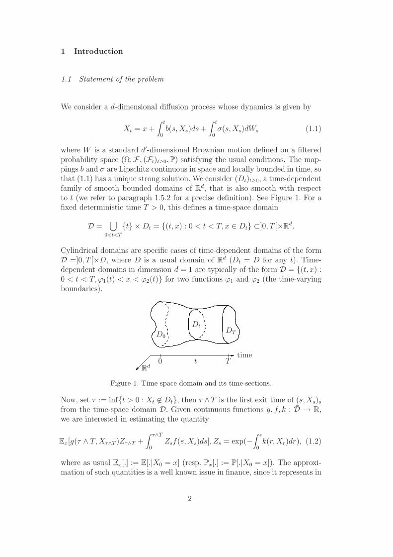
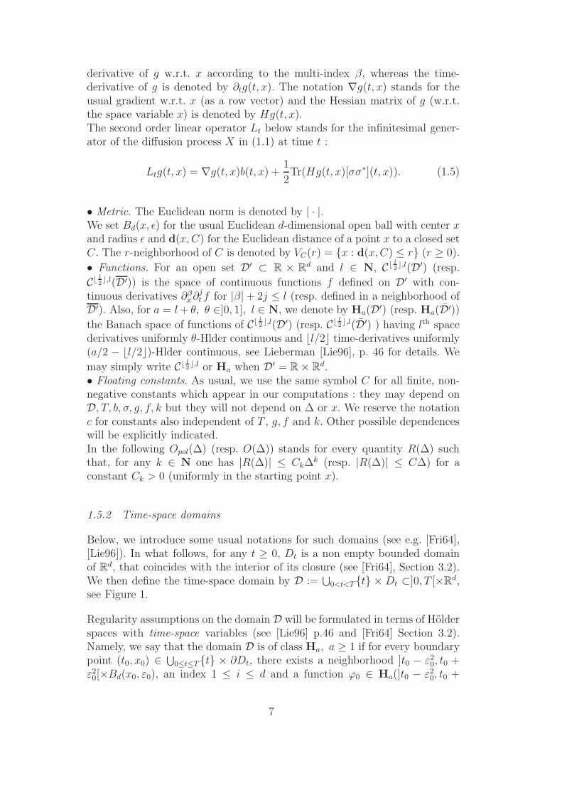
d, that is also smooth with respectto t (we refer to paragraph 1.5.2 for a precise definition). See Figure 1. For afixed deterministic time T > 0, this defines a time-space domain

D =⋃

0<t<T

t × Dt = (t, x) : 0 < t < T, x ∈ Dt ⊂]0, T [×Rd.

Cylindrical domains are specific cases of time-dependent domains of the formD =]0, T [×D, where D is a usual domain of R

d (Dt = D for any t). Time-dependent domains in dimension d = 1 are typically of the form D = (t, x) :0 < t < T, ϕ1(t) < x < ϕ2(t) for two functions ϕ1 and ϕ2 (the time-varyingboundaries).

D0

DtDT

timet0 T

Rd

Figure 1. Time space domain and its time-sections.

Now, set τ := inft > 0 : Xt 6∈ Dt, then τ ∧T is the first exit time of (s, Xs)s

from the time-space domain D. Given continuous functions g, f, k : D → R,we are interested in estimating the quantity

Ex[g(τ ∧ T, Xτ∧T )Zτ∧T +∫ τ∧T

0Zsf(s, Xs)ds], Zs = exp(−

∫ s

0k(r, Xr)dr), (1.2)

where as usual Ex[.] := E[.|X0 = x] (resp. Px[.] := P[.|X0 = x]). The approxi-mation of such quantities is a well known issue in finance, since it represents in

2

this framework the price of a barrier option, see e.g. Andersen and Brotherton-Ratcliffe [ABR96]. These quantities also arise through the Feynman-Kac rep-resentation of the solution of a parabolic PDE with Cauchy-Dirichlet boundaryconditions, see Costantini et al. [CGK06]. They can therefore also be relatedto problems of heat diffusion in time-dependent domains.

We then choose to approximate the expectation in (1.2) by Monte Carlo sim-ulation. This approach is natural and especially relevant compared to deter-ministic methods if the dimension d is large. To this end we approximate thediffusion (1.1) by its Euler scheme with time step ∆ > 0 and discretizationtimes (ti = i∆ = iT/m)i≥0 (m ∈ N∗ so that tm = T ). For t ≥ 0, defineφ(t) = ti for ti ≤ t < ti+1 and introduce

X∆t = x +

∫ t

0b(φ(s), X∆

φ(s))ds +∫ t

0σ(φ(s), X∆

φ(s))dWs. (1.3)

We now associate to (1.3) the discrete exit time τ∆ := infti > 0 : X∆ti

/∈ Dti.Approximating the functional Vτ := g(τ ∧ T, Xτ∧T )Zτ∧T +

∫ τ∧T0 Zsf(s, Xs) ds

by

V ∆τ∆ := g(τ∆ ∧ T, X∆

τ∆∧T )Z∆τ∆∧T +

∫ τ∆∧T

0Z∆

φ(s)f(φ(s), X∆φ(s))ds

with Z∆t = e

−∫ t

0k(φ(r),X∆

φ(r))dr

,

we introduce the quantity

Err(T, ∆, g, f, k, x) = Ex[V∆τ∆ − Vτ ] (1.4)

that will be referred to as the weak error.

Note that in V ∆τ∆ , on τ∆ ≤ T g is a.s. not evaluated on the side part

⋃

0≤t≤Tt×∂Dt of the boundary (g must be understood as a function definedin a neighborhood of the boundary). At first sight, this approximation canseem coarse. Anyhow, it does not affect the convergence rate and really reducesthe computational cost with respect to the alternative that would consist intaking the projection on ∂D. It is a commonly observed phenomenon thatthe error is positive when g is positive (overestimation of Ex(Vτ )), becausewe neglect the possible exits between two discrete times: see Boyle and Lau[BL94], Baldi [Bal95], Gobet and Menozzi [GM04]. In addition, it is knownthat the error is of order ∆1/2: see [GM04] for lower bound results, see [GM07]for upper bounds in the more general case of It processes. But so far, thederivation of an error expansion Ex[V

∆τ∆ − Vτ ] = C

√∆ + o(

√∆) had not been

established: this is one of the intermediary results of the current work (seeTheorem 4).

Our goal goes beyond this result, by designing a simple and very efficientimproved procedure. We propose to stop the Euler scheme at its exit of a

3

∂Dt D∆

t

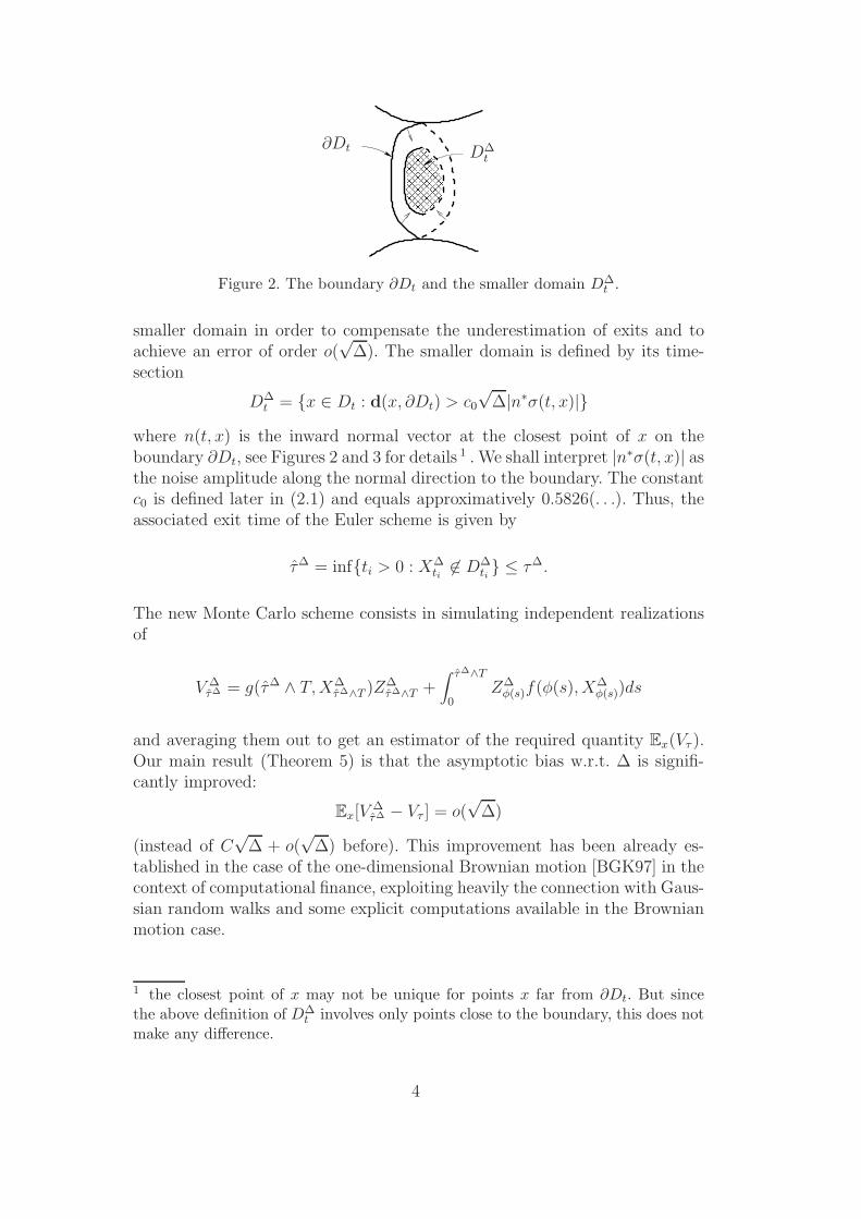
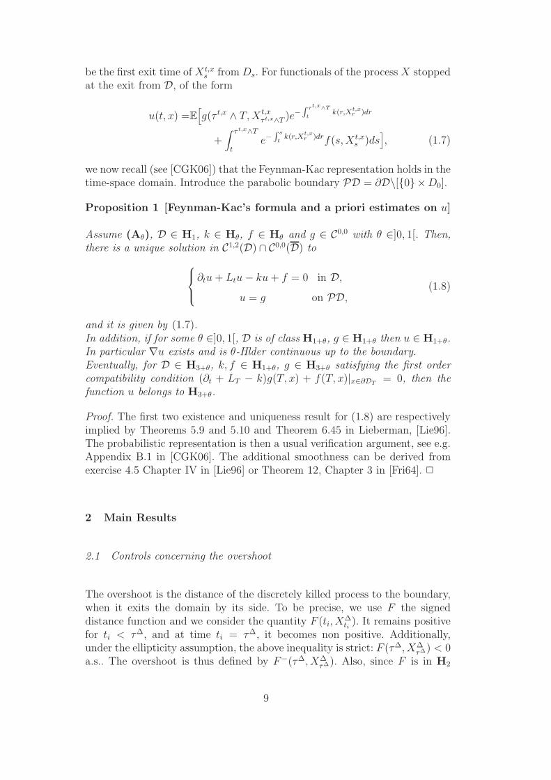
Figure 2. The boundary ∂Dt and the smaller domain D∆t .

smaller domain in order to compensate the underestimation of exits and toachieve an error of order o(

√∆). The smaller domain is defined by its time-

section

D∆t = x ∈ Dt : d(x, ∂Dt) > c0

√∆|n∗σ(t, x)|

where n(t, x) is the inward normal vector at the closest point of x on theboundary ∂Dt, see Figures 2 and 3 for details 1 . We shall interpret |n∗σ(t, x)| asthe noise amplitude along the normal direction to the boundary. The constantc0 is defined later in (2.1) and equals approximatively 0.5826(. . .). Thus, theassociated exit time of the Euler scheme is given by

τ∆ = infti > 0 : X∆ti6∈ D∆

ti ≤ τ∆.

The new Monte Carlo scheme consists in simulating independent realizationsof

V ∆τ∆ = g(τ∆ ∧ T, X∆

τ∆∧T )Z∆τ∆∧T +

∫ τ∆∧T

0Z∆

φ(s)f(φ(s), X∆φ(s))ds

and averaging them out to get an estimator of the required quantity Ex(Vτ ).Our main result (Theorem 5) is that the asymptotic bias w.r.t. ∆ is signifi-cantly improved:

Ex[V∆τ∆ − Vτ ] = o(

√∆)

(instead of C√

∆ + o(√

∆) before). This improvement has been already es-tablished in the case of the one-dimensional Brownian motion [BGK97] in thecontext of computational finance, exploiting heavily the connection with Gaus-sian random walks and some explicit computations available in the Brownianmotion case.

1 the closest point of x may not be unique for points x far from ∂Dt. But sincethe above definition of D∆

t involves only points close to the boundary, this does notmake any difference.

4

1.2 Contribution of the paper

To achieve the results in the current very general framework, we combineseveral ingredients (which correspond to the main steps of the proofs).

(1) We first expand the error Ex[V∆τ∆ − Vτ ] related to the use of the dis-

crete Euler scheme in the domain D. Although this issue deserved manystudies in the literature, the expansion results are new. We prove that itrelies on the study of the weak convergence of the triplet (exit time, posi-tion at exit time, renormalized overshoot at exit time), that is (τ∆, X∆

τ∆ ,∆−1/2d(X∆

τ∆ , ∂Dτ∆)), as ∆ goes to 0. This weak convergence result is cru-cial in this work and it is new (see Theorem 3).Then, combining this with sharp techniques of error analysis, we derivean expansion of the form Err(T, ∆, g, f, k, x) = C

√∆ + o(∆) in the very

general framework of stopped diffusions in time-dependent domains.(2) Second, we analyse the impact of the boundary shifting, in the continuous

time problem (see paragraph 2.3.2). This is related to the differentiabilityof Ex(Vτ ) w.r.t. the boundary and it has been addressed in [CGK06]. Weapply directly their results. Then, we obtain the global error estimate ofthe boundary correction procedure (Theorem 5).

We mention that the previous results about the error expansion and correctionstill hold in the stationary setting, see Section 4, which also seems to be new.A numerical application is discussed in Section 5. Complementary tests arepresented in [Gob09], showing that the boundary correction procedure is verygeneric and seems to work without Markovian property for X. This featurewill be investigated in further research.

Let us finally mention that we could also consider the diffusion process dis-cretely stopped: expansion and correction results below would remain thesame.

1.3 Comparison with results in literature

Up to now, the behavior of (1.4) had mainly been analysed for cylindricaldomains, in the killed case, without source and potential terms (i.e. whenthe error writes Err(T, ∆, g, 0, 0, x) = Ex[g(X∆

T )1τ∆>T ]−Ex[g(XT )1τ>T ]). Letus first mention the work of Broadie et al. [BGK97], who first derived theboundary shifting procedure in the one dimensional geometric Brownian mo-tion setting (Black and Scholes model). In [Gob00] and [GM04], it had beenshown that, under some (hypo)ellipticity conditions on the coefficients andsome smoothness of the domain and the coefficients, Err(T, ∆, g, 0, 0, x) waslower and upper bounded at order 1/2 w.r.t. the time-step ∆. Also, an expan-

5

sion result for the killed Brownian motion in a cone as well as the associatedcorrection procedure are available in [Men06].

All these works emphasize that the crucial quantity to analyse in order toobtain an expansion is the overshoot above the spatial boundary of the dis-crete process. In the Brownian one-dimensional framework such analysis goesback to Siegmund [Sie79] and Siegmund and Yuh [SY82]. Also a non linearrenewal theory for random walk, i.e. for a curved boundary, had been de-veloped by Siegmund and al., see [Sie85] and references therein, Woodroofe[Woo82] and Zhang [Zha88]. We manage to extend their results to obtain theasymptotic distribution of the overshoot of the Euler scheme, see Sections 2and 3. Concerning the asymptotics of the overshoot of stochastic processes, letus mention the works of Alsmeyer [Als94] or Fuh and Lai [FL01] for ergodicMarkov chains and Doney and Kyprianou for Lvy processes [DK06]. Theseworks are all based on renewal arguments.

Finally, for simulating stopped diffusions we also mention the alternative tech-nique based on Random Walks on Spheres. This method allows to derive abound for the weak error associated to the approximation of E[Vτ ] in the ellip-tic setting for a cylindrical domain, see Milstein [Mil97]. The same approachhas also been exploited to obtain some strong error or pathwise bounds for abounded time-space cylindrical domain, see Milstein and Tretyakov [MT99].Recently, Deaconu and Lejay [DL06] have developed similar algorithms, butbased on random walks on rectangles. However, computationally speaking,our approach is presumably more direct.

1.4 Outline of the paper

Notations and assumptions used throughout the paper are stated in Section1.5. In Section 2 we give our main results concerning the asymptotics of theovershoot, the error expansion and the boundary correction. These resultsare proved in Section 3, which is the technical core of the paper. Eventually,Section 4 deals with the stationary extension of our results. We still manage toobtain an expansion and a correction for elliptic PDEs. Some technical resultsare postponed to the Appendix.

1.5 General notation and assumptions

1.5.1 Miscellaneous

• Differentiation. For smooth functions g(t, x), we denote by ∂βxg(t, x) the

6

derivative of g w.r.t. x according to the multi-index β, whereas the time-derivative of g is denoted by ∂tg(t, x). The notation ∇g(t, x) stands for theusual gradient w.r.t. x (as a row vector) and the Hessian matrix of g (w.r.t.the space variable x) is denoted by Hg(t, x).The second order linear operator Lt below stands for the infinitesimal gener-ator of the diffusion process X in (1.1) at time t :

Ltg(t, x) = ∇g(t, x)b(t, x) +1

2Tr(Hg(t, x)[σσ∗](t, x)). (1.5)

• Metric. The Euclidean norm is denoted by | · |.We set Bd(x, ǫ) for the usual Euclidean d-dimensional open ball with center xand radius ǫ and d(x, C) for the Euclidean distance of a point x to a closed setC. The r-neighborhood of C is denoted by VC(r) = x : d(x, C) ≤ r (r ≥ 0).

• Functions. For an open set D′ ⊂ R × Rd and l ∈ N, C⌊ l

2⌋,l(D′) (resp.

C⌊ l2⌋,l(D′)) is the space of continuous functions f defined on D′ with con-

tinuous derivatives ∂βx∂j

t f for |β| + 2j ≤ l (resp. defined in a neighborhood ofD′). Also, for a = l + θ, θ ∈]0, 1], l ∈ N, we denote by Ha(D′) (resp. Ha(D′))

the Banach space of functions of C⌊ l2⌋,l(D′) (resp. C⌊ l

2⌋,l(D′) ) having lth space

derivatives uniformly θ-Hlder continuous and ⌊l/2⌋ time-derivatives uniformly(a/2 − ⌊l/2⌋)-Hlder continuous, see Lieberman [Lie96], p. 46 for details. We

may simply write C⌊ l2⌋,l or Ha when D′ = R × R

d.• Floating constants. As usual, we use the same symbol C for all finite, non-negative constants which appear in our computations : they may depend onD, T, b, σ, g, f, k but they will not depend on ∆ or x. We reserve the notationc for constants also independent of T , g, f and k. Other possible dependenceswill be explicitly indicated.In the following Opol(∆) (resp. O(∆)) stands for every quantity R(∆) suchthat, for any k ∈ N one has |R(∆)| ≤ Ck∆

k (resp. |R(∆)| ≤ C∆) for aconstant Ck > 0 (uniformly in the starting point x).

1.5.2 Time-space domains

Below, we introduce some usual notations for such domains (see e.g. [Fri64],[Lie96]). In what follows, for any t ≥ 0, Dt is a non empty bounded domainof R

d, that coincides with the interior of its closure (see [Fri64], Section 3.2).We then define the time-space domain by D :=

⋃

0<t<Tt × Dt ⊂]0, T [×Rd,

see Figure 1.

Regularity assumptions on the domain D will be formulated in terms of Holderspaces with time-space variables (see [Lie96] p.46 and [Fri64] Section 3.2).Namely, we say that the domain D is of class Ha, a ≥ 1 if for every boundarypoint (t0, x0) ∈ ⋃

0≤t≤Tt × ∂Dt, there exists a neighborhood ]t0 − ε20, t0 +

ε20[×Bd(x0, ε0), an index 1 ≤ i ≤ d and a function ϕ0 ∈ Ha(]t0 − ε2

0, t0 +

7

ε20[×Bd−1((x

10, ..., x

i−10 , xi+1

0 , ..., xd0), ε0) s.t.

∪0≤t≤T t × ∂Dt

∩

]t0 − ε20, t0 + ε2

0[×Bd(x0, ε0)

:= (t, x) ∈ (]t0 − ε20, t0 + ε2

0[∩[0, T ]) × Bd(x0, ε0) :

xi = ϕ0(t, x1, ..., xi−1, xi+1, ..., xd).

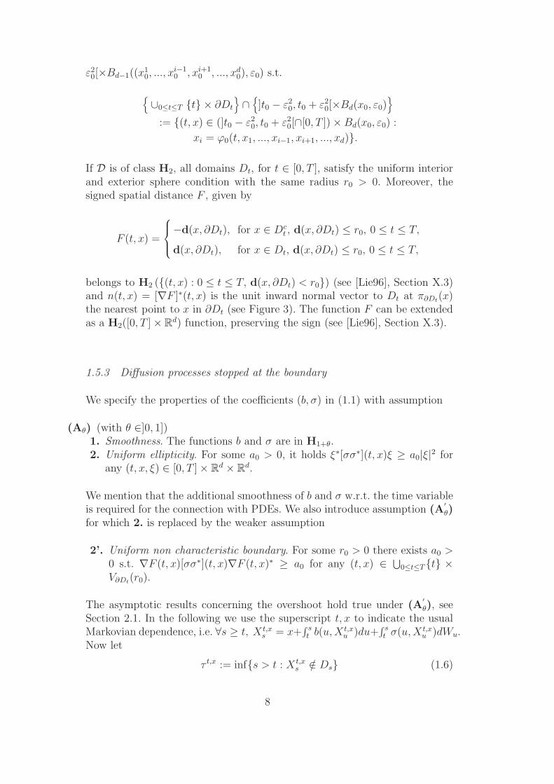
If D is of class H2, all domains Dt, for t ∈ [0, T ], satisfy the uniform interiorand exterior sphere condition with the same radius r0 > 0. Moreover, thesigned spatial distance F , given by

F (t, x) =

−d(x, ∂Dt), for x ∈ Dct , d(x, ∂Dt) ≤ r0, 0 ≤ t ≤ T,

d(x, ∂Dt), for x ∈ Dt, d(x, ∂Dt) ≤ r0, 0 ≤ t ≤ T,

belongs to H2 ((t, x) : 0 ≤ t ≤ T, d(x, ∂Dt) < r0) (see [Lie96], Section X.3)and n(t, x) = [∇F ]∗(t, x) is the unit inward normal vector to Dt at π∂Dt(x)the nearest point to x in ∂Dt (see Figure 3). The function F can be extendedas a H2([0, T ] × R

d) function, preserving the sign (see [Lie96], Section X.3).

1.5.3 Diffusion processes stopped at the boundary

We specify the properties of the coefficients (b, σ) in (1.1) with assumption

(Aθ) (with θ ∈]0, 1])1. Smoothness. The functions b and σ are in H1+θ.2. Uniform ellipticity. For some a0 > 0, it holds ξ∗[σσ∗](t, x)ξ ≥ a0|ξ|2 for

any (t, x, ξ) ∈ [0, T ] × Rd × R

d.

We mention that the additional smoothness of b and σ w.r.t. the time variableis required for the connection with PDEs. We also introduce assumption (A

′

θ)for which 2. is replaced by the weaker assumption

2’. Uniform non characteristic boundary. For some r0 > 0 there exists a0 >0 s.t. ∇F (t, x)[σσ∗](t, x)∇F (t, x)∗ ≥ a0 for any (t, x) ∈ ⋃

0≤t≤Tt ×V∂Dt(r0).

The asymptotic results concerning the overshoot hold true under (A′

θ), seeSection 2.1. In the following we use the superscript t, x to indicate the usualMarkovian dependence, i.e. ∀s ≥ t, X t,x

s = x+∫ st b(u, X t,x

u )du+∫ st σ(u, X t,x

u )dWu.Now let

τ t,x := infs > t : X t,xs /∈ Ds (1.6)

8

be the first exit time of X t,xs from Ds. For functionals of the process X stopped

at the exit from D, of the form

u(t, x) =E

[

g(τ t,x ∧ T, X t,xτ t,x∧T )e−

∫ τt,x∧T

tk(r,Xt,x

r )dr

+∫ τ t,x∧T

te−∫ s

tk(r,Xt,x

r )drf(s, X t,xs )ds

]

, (1.7)

we now recall (see [CGK06]) that the Feynman-Kac representation holds in thetime-space domain. Introduce the parabolic boundary PD = ∂D\[0×D0].

Proposition 1 [Feynman-Kac’s formula and a priori estimates on u]

Assume (Aθ), D ∈ H1, k ∈ Hθ, f ∈ Hθ and g ∈ C0,0 with θ ∈]0, 1[. Then,there is a unique solution in C1,2(D) ∩ C0,0(D) to

∂tu + Ltu − ku + f = 0 in D,

u = g on PD,(1.8)

and it is given by (1.7).In addition, if for some θ ∈]0, 1[, D is of class H1+θ, g ∈ H1+θ then u ∈ H1+θ.In particular ∇u exists and is θ-Hlder continuous up to the boundary.Eventually, for D ∈ H3+θ, k, f ∈ H1+θ, g ∈ H3+θ satisfying the first ordercompatibility condition (∂t + LT − k)g(T, x) + f(T, x)|x∈∂DT

= 0, then thefunction u belongs to H3+θ.

Proof. The first two existence and uniqueness result for (1.8) are respectivelyimplied by Theorems 5.9 and 5.10 and Theorem 6.45 in Lieberman, [Lie96].The probabilistic representation is then a usual verification argument, see e.g.Appendix B.1 in [CGK06]. The additional smoothness can be derived fromexercise 4.5 Chapter IV in [Lie96] or Theorem 12, Chapter 3 in [Fri64]. 2

2 Main Results

2.1 Controls concerning the overshoot

The overshoot is the distance of the discretely killed process to the boundary,when it exits the domain by its side. To be precise, we use F the signeddistance function and we consider the quantity F (ti, X

∆ti

). It remains positivefor ti < τ∆, and at time ti = τ∆, it becomes non positive. Additionally,under the ellipticity assumption, the above inequality is strict: F (τ∆, X∆

τ∆) < 0a.s.. The overshoot is thus defined by F−(τ∆, X∆

τ∆). Also, since F is in H2

9

(and therefore Lipschitz continuous in time and space), it is easy to see thatF−(τ∆, X∆

τ∆) is of order√

∆ (in Lp-norm for instance). Thus, it is natural tostudy the asymptotics of the rescaled overshoot

∆−1/2F−(τ∆, X∆τ∆).

Adapting the proof of Proposition 6 in [GM04] to our time-dependent context,see also the proof of Proposition 15 for a simpler version, one has the followingproposition.

Proposition 2 (Tightness of the overshoot) Assume (A′

θ), and that Dis of class H2. Then, for some c > 0 one has

sup∆>0,s∈[0,T ]

Ex[exp(c[∆−1/2F−(s ∧ τ∆, X∆s∧τ∆)]2)] < +∞.

It is quite plain to prove, by pathwise convergence of X∆ towards X on com-pact sets, that (τ∆ ∧T, X∆

τ∆∧T ) converges in probability to (τ ∧T, Xτ∧T ). Thenext theorem also includes the rescaled overshoot.

Theorem 3 (Joint limit laws associated to the overshoot) Assume (A′

θ),and that D is of class H2. Let ϕ be a continuous function with compact support.For all t ∈ [0, T ], x ∈ D0, y ≥ 0,

Ex[1τ∆≤tZ∆τ∆ϕ(X∆

τ∆)1F−(τ∆,X∆τ∆

)≥y√

∆] −→∆→0

Ex

[

1τ≤tZτϕ(Xτ )(

1 − H(y/|∇Fσ(τ, Xτ)|))]

with H(y) := (E0[sτ+ ])−1∫ y0 P0[sτ+ > z]dz and s0 := 0, ∀n ≥ 1, sn :=

∑ni=1 Gi,

the Gi being i.i.d. standard centered normal variables, τ+ := infn ≥ 0 : sn >0.

In other words, (τ∆, X∆τ∆ , ∆−1/2F−(τ∆, X∆

τ∆)) weakly converges to(τ, Xτ , |∇Fσ(τ, Xτ)|Y ) where Y is a random variable independent of (τ, Xτ ),and which cumulative function is equal to H . Actually, Y has the asymptoticlaw of the renormalized Brownian overshoot. In the following analysis, themean of the overshoot is an important quantity and it is worth noting that

one has E(Y ) =E0[s2

τ+ ]

2E0[sτ+ ]:= c0. One knows from [Sie79] that

c0 = −ζ(1/2)√2π

= 0.5826... (2.1)

The above theorem is the crucial tool in the derivation of our main results.The proof is given in Section 3.1.

10

2.2 Error expansion and boundary correction

For notational convenience introduce for x ∈ D0,

u(D) = Ex(g(τ ∧ T, Xτ∧T )Zτ∧T +∫ τ∧T

0Zsf(s, Xs)ds),

u∆(D) = Ex(g(τ∆ ∧ T, X∆τ∆∧T )Z∆

τ∆∧T +∫ τ∆∧T

0Z∆

φ(s)f(φ(s), X∆φ(s))ds).

Theorem 4 (First order expansion) Under (Aθ), for a domain of classH2, g ∈ H1+θ, k, f ∈ H1+θ and for ∆ small enough

Err(T, ∆, g, f, k, x) = u∆(D) − u(D)

= c0

√∆Ex(1τ≤T Zτ (∇u −∇g)(τ, Xτ) · ∇F (τ, Xτ)|∇Fσ(τ, Xτ)|) + o(

√∆),

where c0 is defined in (2.1).

Define now a smaller domain D∆ ⊂ D, which time-section is given by D∆t =

x ∈ Dt : d(x, ∂Dt) > c0

√∆|∇Fσ(t, x)|, see Figure 2. Introduce the exit

time of the Euler scheme from this smaller domain: τ∆ = infti > 0 : X∆ti

6∈D∆

ti ≤ τ∆. The boundary correction procedure consists in simulating

g(τ∆ ∧ T, X∆τ∆∧T )Z∆

τ∆∧T +∫ τ∆∧T

0Z∆

φ(s)f(φ(s), X∆φ(s))ds. (2.2)

As above, we do not compute any projection on the boundary. We denote theexpectation of (2.2) by u∆(D∆). One has:

Theorem 5 (Boundary correction) Under the assumptions of Theorem 4,if we additionally suppose ∇F (., .)|∇Fσ(., .)| is in C1,2, then one has:

u∆(D∆) − u(D) = o(√

∆).

The additional assumption is due to technical considerations to ensure thatthe modified domain D∆ is also of class H2. It is automatically fulfilled fordomains of class C3 and σ in C1,2.

2.3 Proof of Theorems 4 and 5

2.3.1 Error expansion

By usual weak convergence arguments, Theorem 4 is a direct consequenceof Proposition 2 (tightness), Theorem 3 (joint limit laws associated to the

11

overshoot) and Theorem 6 below.

Theorem 6 (First order approximation) Under the assumptions of The-orem 4, one has

u∆(D) − u(D) = o(√

∆)+

Ex(1τ∆≤T Z∆τ∆(∇u −∇g)(τ∆, π∂D

τ∆(X∆

τ∆)) · ∇F (τ∆, X∆τ∆)F−(τ∆, X∆

τ∆)).

Remark 7 In the above statement, we use projections on a non convex set,which needs a clarification. With the notation of Section 1.5.2, introduce τ r0 :=infs > 0 : X∆

s /∈ VDs(r0). For s ∈ [0, τ r0 ] the projection πDs(X∆

s ) is uniquelydefined by

πDs(X∆

s ) = X∆s + (∇F )∗(s, X∆

s )F−(s, X∆s ), (2.3)

see Figure 3. Large deviation arguments (see Lemma 8 below) also give Px[τr0 ≤

τ∆ ≤ T ] = Opol(∆). Thus, in the following, for s ≥ τ r0, πDs(X∆

s ) andπ∂Ds(X

∆s ) denote an arbitrary point on ∂Ds. This choice yields an exponen-

tially small contribution in our estimates.

x

π∂Dt(x) = yx

F−(t, x)n(t, y) = [∇F ]∗(t, x)

Figure 3. Orthogonal projection π∂Dt(x) of x /∈ Dt onto the bound-ary ∂Dt and the related signed distance F (t, x). Here F (t, x) < 0 andd(x, ∂Dt) = |F (t, x)| = F−(t, x).

Proof. Denote e∆ := u∆(D) − u(D) the above error. Write now

e∆ =Ex[g(τ∆ ∧ T, X∆τ∆∧T )Z∆

τ∆∧T − g(τ∆ ∧ T, πDτ∆∧T

(X∆τ∆∧T ))Z∆

τ∆∧T ]

+

Ex[g(τ∆ ∧ T, πDτ∆∧T

(X∆τ∆∧T ))Z∆

τ∆∧T +∫ τ∆∧T

0Z∆

φ(s)f(φ(s), X∆φ(s))ds]

− u(0, X∆0 )

:=e∆1 + e∆

2 .

12

We introduce here the projection for the error analysis. From (2.3) and Propo-sition 2, a Taylor expansion yields

e∆1 = − Ex[1τ∆≤T Z∆

τ∆∇g(τ∆, π∂Dτ∆

(X∆τ∆)) · ∇F (τ∆, X∆

τ∆)F−(τ∆, X∆τ∆)]

+ O(∆(1+θ)/2). (2.4)

In the following, we write UE= V (resp U

E

≤ V ) when the equality between Uand V holds in mean up to a Opol(∆) (resp. Ex(U) ≤ Ex(V ) + Opol(∆)). Wealso use the notation U = O(V ) between two random variables U and V iffor a constant C, one has |U | ≤ C|V |. Because g(τ∆ ∧ T, πD

τ∆∧T(X∆

τ∆∧T )) =

u(τ∆ ∧ T, πDτ∆∧T

(X∆τ∆∧T )), we can write a telescopic summation:

e∆2

E=(

∑

0≤ti<τ∆∧T

u(ti+1, πDti+1(X∆

ti+1))Z∆

ti+1

− u(ti, πDti(X∆

ti))Z∆

ti+ Z∆

tif(ti, X

∆ti

)∆)

1τr0>τ∆∧T

E=(

∑

0≤ti<T

1ti<τ∆

[

u(ti+1, πDti+1(X∆

ti+1))Z∆

ti+1

−u(ti, X∆ti

)Z∆ti

+ Z∆ti

f(ti, X∆ti

)∆])

1τr0>τ∆∧T

since for ti < τ∆, X∆ti

∈ Dti and thus πDti(X∆

ti) = X∆

ti. To proceed, the

key idea is to introduce on the event ti < τ∆, the partition F (ti, X∆ti

) ∈(0, 2∆

12(1−ε)] ∪ F (ti, X

∆ti

) > 2∆12(1−ε) := Aε

ti∪ (Aε

ti)C , ε > 0. This allows to

split the cases for which X∆ti

is close or not to the boundary ∂Dti . Lemma 8

ensures that (X∆s )s∈[ti,ti+1] stayed in B(X∆

ti, ∆

12(1−ε)) with a probability expo-

nentially close to one. Then, on (Aεti)C , the smoothness of the domain yields

1(Aεti

)C P[X∆ti+1

∈ Dti+1|Fti] = 1 − O(exp(−c∆−ε)), see Proposition 19 for a

proof of this claim. On the other hand, on Aεti, X∆

tiis sufficiently close to the

boundary to make the contribution of the overshoot at time ti+1 significantfor the error analysis. Write:

e∆2

E=(

∑

0≤ti<T

1ti<τ∆

1Aεti

[

u(ti+1, πDti+1(X∆

ti+1))Z∆

ti+1

−u(ti, X∆ti

)Z∆ti

+ Z∆ti

f(ti, X∆ti

)∆]

+ 1(Aεti

)C1∀s∈[ti,ti+1], X∆s ∈B(X∆

ti,∆

12(1−ε))

[

u(ti+1, X∆ti+1

)Z∆ti+1

−u(ti, X∆ti

)Z∆ti

+ Z∆ti

f(ti, X∆ti

)∆])

1τr0>τ∆∧T := e∆21 + e∆

22. (2.5)

Let us first deal with e∆21. In our framework, u is (1 + θ)/2-Holder continuous

in time and ∇u is θ-Holder continuous in space on a neighborhood of D. A

13

Taylor expansion at order one and the equality (2.3) give

e∆21

E=(

∑

0≤ti<T

1ti<τ∆1Aεti

[

Z∆ti∇u(ti, X

∆ti

) · ∇F (ti+1, X∆ti+1

)F−(ti+1, X∆ti+1

)

+O(|F−(ti+1, X∆ti+1

)|1+θ) + O(|X∆ti+1

− X∆ti|1+θ) + O(∆

1+θ2 )])

1τr0>τ∆∧T

E=(

1τ∆≤T Z∆τ∆∇u(τ∆, X∆

τ∆) · ∇F (τ∆, X∆τ∆)F−(τ∆, X∆

τ∆)

+∑

0≤ti<T

1ti<τ∆1Aεti

[

O(|F−(ti+1, X∆ti+1

)|1+θ) + O(|X∆ti+1

− X∆ti|1+θ)

+ O(|X∆ti+1

− X∆ti|θF−(ti+1, X

∆ti+1

)) + O(∆1+θ2 )])

1τr0>τ∆∧T

where we used once again Lemma 8 for the last equality. Standard argumentsyield E[|X∆

ti+1−X∆

ti|p|Fti] = O(∆

p2 ) for any p > 0 and E[|F−(ti+1, X

∆ti+1

)|p|Fti] =

E[|F−(ti+1, X∆ti+1

) − F−(ti, X∆ti

)|p|Fti] = O(∆p2 ) on ti < τ∆. Thus, we can

now rewrite

e∆21

E=(

1τ∆≤T Z∆τ∆∇u(τ∆, π∂D

τ∆(X∆

τ∆)) · ∇F (τ∆, X∆τ∆)F−(τ∆, X∆

τ∆))

1τr0>τ∆∧T

+ e∆211,

e∆211

E=(

∑

0≤ti<T

1ti<τ∆1AεtiO(∆

1+θ2 ))

1τr0>τ∆∧T .

To handle e∆211 the idea is to use the occupation time formula and some sharp

estimates concerning the local time of (F (s, X∆s ))s≤T∧τ∆ in a neighborhood of

the boundary. We have

|e∆211|

E

≤ C∆1+θ2

(

∆−1∫ T∧τ∆

01F (φ(t),X∆

φ(t))∈[0,2∆1/2(1−ε)]dt

)

1τr0>τ∆∧T

E

≤ C∆1+θ2

(

∆−1∫ T∧τ∆

01F (t,X∆

t )∈[−∆1/2(1−ε) ,3∆1/2(1−ε)]dt

)

1τr0>τ∆∧T

E

≤ C∆1+θ2

(

∆−1∫ 3∆1/2(1−ε)

−∆1/2(1−ε)Ly

T∧τ∆(F (., X∆. ))dy

)

1τr0>τ∆∧T ,

where we have used Lemma 8 at the second equality and the uniform ellipticityassumption for the last one. Now an easy adaptation of the proof of Lemma17 [GM04] to our time-dependent domain framework gives

E[LyT∧τ∆(F (., X∆

. ))] ≤ C(|y|+ ∆12 ). (2.6)

Thus, one has |e∆211|

E

≤ C∆1+θ2

− ε2 = o(∆

12 ) for ε small enough. Hence, the above

estimates and Lemma 8 give

e∆21

E=(

1τ∆≤T Z∆τ∆∇u(τ∆, π∂D

τ∆(X∆

τ∆)) · ∇F (τ∆, X∆τ∆)F−(τ∆, X∆

τ∆))

+ o(∆12 ).

(2.7)

14

Let us now turn to e∆22. If g ∈ H3+θ (which implies u ∈ H3+θ in view of Propo-

sition 1), the term e∆22 can be handled with somehow standard techniques.

Namely Taylor like expansions in the spirit of Talay and Tubaro [TT90]. Forsimplicity we handle e∆

22 under the previous smoothness assumption on g andu. The proof under weaker assumptions (g ∈ H1+θ), that involves sharp esti-mates on possibly exploding derivatives of u near the boundary, is postponedto the Appendix. We recall that

e∆22

E=(

∑

0≤ti<T

1ti<τ∆1(Aεti

)C1∀s∈[ti,ti+1], X∆s ∈B(X∆

ti,∆

12 (1−ε))

[

u(ti+1, X∆ti+1

)Z∆ti+1

−u(ti, X∆ti

)Z∆ti

+ Z∆ti

f(ti, X∆ti

)∆])

1τr0>τ∆∧T

For all (s, y) ∈ D introduce the operators Ls,y : C1,2(D) → C(D), ϕ 7→((t, x) 7→ Ls,yϕ(t, x) = ∇ϕ(t, x)b(s, y) + 1

2Tr[Hϕ(t, x)[σσ∗](s, y)]). Recalling

that ∂tu(ti, X∆ti

) + Lti,X∆tiu(ti, X

∆ti

)− ku(ti, X∆ti

) + f(ti, X∆ti

) = 0, Ito’s formula

gives

e∆22

E=(

∑

0≤ti<T

1ti<τ∆1(Aεti

)C1∀s∈[ti,ti+1], X∆

s ∈B(X∆ti

,∆12 (1−ε))

[

∫ ti+1

ti(Z∆

s − Z∆ti

)(∂s + Lti,X∆ti− k(ti, X

∆ti

))u(s, X∆s )ds

+ Z∆ti

∫ ti+1

ti

[(

∂s + Lti,X∆ti− k(ti, X

∆ti

))

u(s, X∆s )

−(

∂s + Lti,X∆ti− k(ti, X

∆ti

))

u(ti, X∆ti

))]

ds

+ Mti,ti+1

])

1τr0>τ∆∧T , (2.8)

where for all v ∈ [ti, ti+1], Mti,v :=∫ v

tiZ∆

s ∇u(s, X∆s )σ(ti, X

∆ti

)dWs is a square-

integrable martingale term. Note that in this definition, in whole generality,Mti,v is not stopped at the exit time τti := infs ≥ ti : X∆

s 6∈ Ds. If τti ≤ ti+1

(which happens with exponentially small probability on (Aεti)C), the term

∇u(s, X∆s ), s ∈ [τti , ti+1] in Mti,ti+1

has to be understood as the smooth exten-sion of ∇u to the whole space. In particular this extension remains bounded.Now, we derive from Lemma 8

Ex[(

∑

0≤ti<T

1ti<τ∆1(Aεti

)C1∀s∈[ti,ti+1], X∆s ∈B(X∆

ti,∆

12(1−ε))

Mti,ti+1

])

1τr0>τ∆∧T ]

= Ex[∑

0≤ti<T

1ti<τ∆1(Aεti

)CMti,ti+1] + Opol(∆) = Opol(∆).

15

We can thus neglect the contribution of the martingale terms in (2.8). We nowdevelop the other quantities in (2.8) with Taylor integral formulas to derive

∫ ti+1

ti(Z∆

s − Z∆ti

)(∂s + Lti,X∆ti− k(ti, X

∆ti

))u(s, X∆s )ds

=O(

∆2(|u|∞ + |∇u|∞ + |∂tu|∞ + |D2u|∞))

,∫ ti+1

ti(∂tu(s, X∆

s ) − ∂tu(ti, X∆ti

))ds

=∫ ti+1

ti∇∂tu(ti, X

∆ti

)σ(ti, X∆ti

)(Ws − Wti)ds

+ O(

∆1+ 1+θ2 [∂tu]t, 1+θ

2+ ∆2|∇∂tu|∞ + ∆ sup

s∈[ti,ti+1]|X∆

s − X∆ti|1+θ[∇∂tu]x,θ

)

,

∫ ti+1

ti(Lti,X∆

tiu(s, X∆

s ) − Lti,X∆tiu(ti, X

∆ti

))ds

=∫ ti+1

ti〈Hu(ti, X

∆ti

)σ(ti, X∆ti

)(Ws − Wti), b(ti, X∆ti

)〉ds

+1

2

∫ ti+1

tiTr(

(D3u(ti, X∆ti

)σ(ti, X∆ti

)(Ws − Wti)) · a(ti, X∆ti

))

ds

+ O(

∆2|D2u|∞ + |D3u|∞ + |∂t∇u|∞ + ∆1+ 1+θ2 [D2u]t, 1+θ

2

+ ∆|D3u|∞ sups∈[ti,ti+1]

|X∆s − X∆

ti|2 + ∆ sup

s∈[ti,ti+1]|X∆

s − X∆ti|1+θ[D3u]x,θ

)

,

k(ti, X∆ti

)∫ ti+1

ti(u(s, X∆

s ) − u(ti, X∆ti

))ds

=k(ti, X∆ti

)∫ ti+1

ti∇u(ti, X

∆ti

)σ(ti, X∆ti

)(Ws − Wti)ds

+ O(

∆2(|∂tu|∞ + |∇u|∞) + ∆|D2u|∞ sups∈[ti,ti+1]

|X∆s − X∆

ti|2)

, (2.9)

where [·]t,α, [·]x,α, α ∈ (0, 1] denote respectively the Holder norms of order αin time and space (see Chapter IV Section 1 p. 46 in [Lie96] for a precisedefinition).

Hence, bringing together our estimates and exploiting the relations betweenthe spatial and time derivatives for u (through the PDE), from (2.8) and (2.9)

16

we derive

e∆22

E=(

∑

0≤ti<T

1ti<τ∆1(Aεti

)C1∀s∈[ti,ti+1], X∆s ∈B(X∆

ti,∆

12(1−ε))

[

O(

∆21 + |u|∞ + |∇u|∞ + |D2u|∞ + |D3u|∞)

+ O(

∆1+ 1+θ2 1 + |u|∞ + |∇u|∞ + |D2u|∞ + |D3u|∞ + [D2u]t, 1+θ

2)

+ O(

∆ sups∈[ti,ti+1]

|X∆s − X∆

ti|1+θ1 + |u|∞ + |∇u|∞ + |D2u|∞ + |D3u|∞ + [D3u]x,θ

)

+ O(

∆ sups∈[ti,ti+1]

|X∆s − X∆

ti|2|D2u|∞ + |D3u|∞

)

+ Mti,ti+1

])

1τr0>τ∆∧T , (2.10)

where Mti,ti+1denotes the sum of the terms involving the Brownian increment

(Ws − Wti)s∈[ti,ti+1] in the above equations (2.9). Under our current assump-tion, i.e. u ∈ H3+θ, all the norms appearing in (2.10) and all the derivativesappearing in the (Mti,ti+1

)0≤ti<T are bounded. Hence,

1ti<τ∆1(Aεti

)C E[1∀s∈[ti,ti+1], X∆s ∈B(X∆

ti,∆

12 (1−ε))

Mti,ti+11τr0>τ∆∧T |Fti ]

=1ti<τ∆1(Aεti

)C E[Mti,ti+1|Fti] + Opol(∆) = Opol(∆), (2.11)

|e∆22|

E

≤C∆1+θ2 . (2.12)

Plug (2.7) and (2.12) into (2.5). The statement is derived from (2.4) and (2.5).We specify in the Appendix how to complete the proof from a sharper versionof (2.10) deriving from (2.8), when g ∈ H1+θ. 2

2.3.2 Boundary Correction

One has

u∆(D∆) − u(D) = [u∆(D∆) − u(D∆)] + [u(D∆) − u(D)]. (2.13)

(1) The first contribution in (2.13) has been previously analysed in Theorem4, except that the domain D∆ depends on ∆. We can show that it is equalto c0

√∆E(1τ≤T Zτ (∇u−∇g)(τ, Xτ) · ∇F (τ, Xτ)|∇Fσ(τ, Xτ )|) + o(

√∆).

We briefly sketch the proof of this assertion, which is done in two steps.For this, set u∆ = u(D∆) for the solution of the PDE in the domain D∆.• Step 1. It is well known that all PDE estimates depend only on bounds

on the derivatives of the level set functions (ϕ0) arising in the definitionof the time-dependent domains (see section 1.5.2), and on the boundson the derivatives of data g, f and k. Hence, since D∆ is a small per-turbation of class H2 (because ∇F |∇Fσ| has this regularity) of thedomain D of class H2, all PDE estimates on u∆ remain locally uni-form w.r.t. ∆. In addition, u∆ and its gradient converge uniformly to

17

u and ∇u. This argumentation allows us to state that the first orderapproximation theorem holds:

u∆(D∆) − u(D∆) = o(√

∆)+

Ex(1τ∆≤T Z∆τ∆(∇u −∇g)(τ∆, π∂D∆

τ∆(X∆

τ∆)) · ∇F∆(τ∆, X∆τ∆)[F∆]−(τ∆, X∆

τ∆)),

where F∆ and τ∆ are respectively the signed distance to the side of D∆

and the related discrete exit time.• Step 2. The second step is to prove that the analogous version of

Theorem 3 holds, with τ∆ instead of τ∆. Actually, a careful reading ofits proof shows that it is indeed the case, without modification.

(2) Finally, the last term in (2.13) is related to the sensitivity of a Dirichletproblem with respect to the domain. By an application of Theorem 2.2 in[CGK06] with Θ(t, x) = −c0∇F (t, x)|∇Fσ(t, x)| (in C1,2), one gets thatthis contribution equals

−c0

√∆E(1τ≤T Zτ (∇u −∇g)(τ, Xτ) · ∇F (τ, Xτ)|∇Fσ(τ, Xτ )|) + o(

√∆).

This proves that the new procedure has an error o(√

∆). 2

3 Technical results concerning the overshoot

This section is devoted to the proof of Theorem 3. We first state some usefulauxiliary results.

Lemma 8 (Bernstein’s inequality) Assume (Aθ-1). Consider two stop-ping times S, S ′ upper bounded by T with 0 ≤ S ′ − S ≤ Θ ≤ T . Then for anyp ≥ 1, there are some constants c > 0 and C := C((Aθ-1) , T ), such that forany η ≥ 0, one has a.s:

P[ supt∈[S,S′]

|X∆t − X∆

S | ≥ η∣

∣

∣ FS] ≤C exp

(

−cη2

Θ

)

,

E[ supt∈[S,S′]

|X∆t − X∆

S |p∣

∣

∣ FS] ≤CΘp/2.

For a proof of the first inequality we refer to Chapter 3, §3 in [RY99]. The lastinequality easily follows from the first one or from the BDG inequalities.

Lemma 9 (Convergence of exit time) Assume (A′

θ) and that the domainis of class H2. The following convergences hold in probability:

(1) lim∆→0 τ∆ ∧ T = τ ∧ T ;(2) lim∆→0 X∆

τ∆∧T = Xτ∧T ;

18

(3) lim∆→0 supt≤T |X∆φ(t) − Xt| = 0.

The proof of the first two assertions in the case of space-time domain is analo-gous to the case of cylindrical domain (see [GM05]) and thus left to the reader.The last convergence is standard.

The following results are key tools to prove Theorem 3. A similar version isproved in [Sie79], but here, we additionally prove the uniform convergence.

Lemma 10 (Asymptotic independence of the overshoot and the dis-crete exit time). Let W be a standard one dimensional BM. Put x > 0 andconsider the domain D :=]0, T [×]−∞, x[. With the notation of Section 2, forany ε > 0 we have

lim∆−→0

supt∈[0,T ],y≥0,x≥∆1/2−ε

∣

∣

∣P0[τ∆ ≤ t, (Wτ∆ − x) ≤ y

√∆] − P0[τ ≤ t]H(y)

∣

∣

∣ = 0.

(3.1)

If the Euler scheme starts close to the boundary at a small distance d, itsdiscrete exit likely occurs after a time roughly equal to d2. This feature isquantified in the above lemma.

Lemma 11 Assume (A′

θ), and that the domain is of class H2. Let 0 < β <α < 1/2. For all η > 0, there exists C := Cη > 0 s.t. for ∆ small enough,∀s ∈ ∆N ∩ [0, T ] and ∀x ∈ V∂Ds(∆

α) ∩ Ds, one has

P[τ∆ ∧ T ≥ ∆2β |X∆s = x] ≤ C(∆α−β−η + ∆β),

where τ∆ := infti > s : X∆ti

/∈ Dti.

Lemma 12 Assume (A′

θ), and that the domain is of class H2. There existsC > 0, such that ∀s ∈ ∆N ∩ [0, T ], ∀x ∈ Ds, ∀t ∈ [s, T ] and ∀b ≥ a ≥ 0, onehas

P[τ∆ ≤ t, ∆−1/2F−(τ∆, X∆τ∆) ∈ [a, b]|X∆

s = x] ≤C(

(b − a) + ∆1/4)

where τ∆ is shifted as in the previous lemma.

The proof of these three lemmas is postponed to Section 3.2.

We mention that if σσ∗ is uniformly elliptic, Lemma 12 is valid without the∆1/4 (see the proof for details). In that case, it means that the law of therenormalized overshoot is absolutely continuous w.r.t. the Lebesgue measureon R

+, with a bounded density. This is also true at the limit, in view ofTheorem 3.

19

3.1 Proof of Theorem 3

Consider first the case D =]0, T [×D where D is a half space. The theoremin the case of BM is then a direct consequence of Lemma 10. Now to dealwith the Euler scheme, we introduce a first neighborhood whose distance tothe boundary goes to 0 with ∆ at a speed lower than ∆1/2 (below, the speedis tuned by a parameter α, see Figure 4). The characteristic exit time for astarting point in this neighborhood is short (Lemma 11), thus the diffusioncoefficients are somehow constant and we are almost in the BM framework.Also, a second localization w.r.t. to the hitting time of this neighborhood guar-antees that up to a rescaling we are far enough from the boundary to applythe renewal arguments needed for the asymptotic law of the overshoot (this istuned by another parameter ε, see Figure 4).For a more general time-space domain of class H2 two additional tools areused: a time-space change of chart and a local half space approximation of thedomain by some tangent hyperplane.For notational convenience, we assume from now on that the time-section do-mains (Dt)t∈[0,T ] are convex so that π∂Dt is always uniquely defined on Dc

t . Tohandle the case of general H2 domains, an additional localization proceduresimilar to the one of Theorem 6 is needed. We leave it to the reader.For the sake of clarity, we also assume k ≡ 0 (Z ≡ 1). This is an easy simpli-fication since owing to Lemma 9, Z∆

τ∆∧T converges to Zτ∧T in L1.

Step 1: preliminary localization. For α < 1/2 specified later on, defineτ∆α := infti > 0 : F (ti, X

∆ti

) ≤ ∆α ≤ τ∆. We aim at studying the conver-gence of

Ψ∆(t, x, y) := Ex[1τ∆≤t,F−(τ∆,X∆τ∆

)≥y√

∆ϕ(X∆τ∆)]

and for this, we define for all 0 ≤ s ≤ t < T (s ∈ ∆N), (x, y) ∈ Rd × R

+

Ψ∆(s, t, x, y) :=P[τ∆ ≤ t, F−(τ∆, X∆τ∆) ≥ y

√∆|X∆

s = x],

A(t, α, ε) :=τ∆α < τ∆, τ∆α < t, F (τ∆α, X∆τ∆α ) ≥ ∆1/2−ε.

Here, ε is a fixed parameter in ]0, 1/2[, such that α < 1/2 − ε (take ε =(α + 1/2)/2 for instance).In the definition of Ψ∆, τ∆ has to be understood as the shifted exit timeinfti > s : X∆

ti/∈ Dti. By Lemma 8, Px[τ

∆ = τ∆α ≤ t] + Px[τ∆α <

t, F (τ∆α, X∆τ∆α ) < ∆1/2−ε] = Opol(∆) using α < 1/2 − ε. Hence,

Ψ∆(t, x, y) =Ex[1A(t,α,ε),F−(τ∆,X∆τ∆

)≥y√

∆ϕ(X∆τ∆)1τ∆≤t] + Opol(∆)

=Ex[1A(t,α,ε),F−(τ∆,X∆τ∆

)≥y√

∆(ϕ(X∆τ∆) − ϕ(X∆

τ∆α ))1τ∆≤t]

+ Ex[1A(t,α,ε)ϕ(X∆τ∆α )Ψ∆(τ∆α , t, X∆

τ∆α , y)] + Opol(∆).

The first term in the right hand side above converges to 0, using the conver-

20

gence in probability of |X∆τ∆∧T −X∆

τ∆α∧T | to 0 (analogously to Lemma 9). Thisgives

Ψ∆(t, x, y) = Ex[1A(t,α,ε)ϕ(X∆τ∆α )Ψ∆(τ∆α, t, X∆

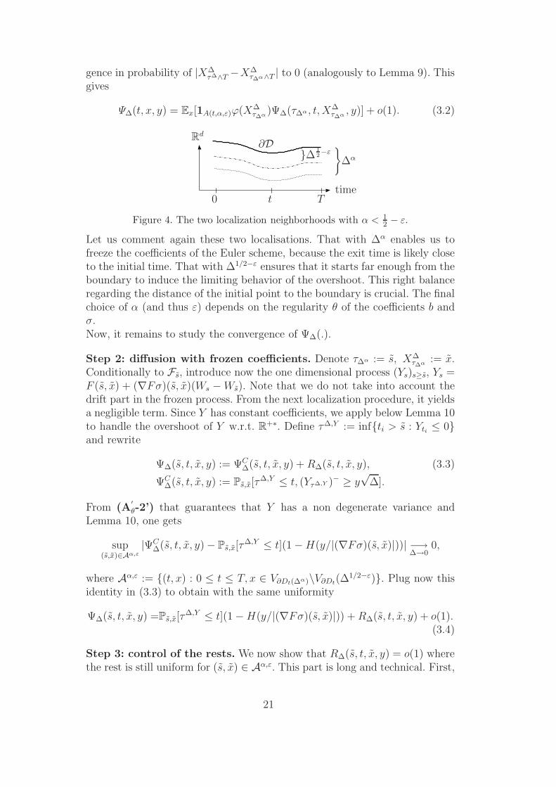
τ∆α , y)] + o(1). (3.2)

t0 T

Rd

time

∂D∆ 1

2−ε

∆α

Figure 4. The two localization neighborhoods with α < 12 − ε.

Let us comment again these two localisations. That with ∆α enables us tofreeze the coefficients of the Euler scheme, because the exit time is likely closeto the initial time. That with ∆1/2−ε ensures that it starts far enough from theboundary to induce the limiting behavior of the overshoot. This right balanceregarding the distance of the initial point to the boundary is crucial. The finalchoice of α (and thus ε) depends on the regularity θ of the coefficients b andσ.Now, it remains to study the convergence of Ψ∆(.).

Step 2: diffusion with frozen coefficients. Denote τ∆α := s, X∆τ∆α := x.

Conditionally to Fs, introduce now the one dimensional process (Ys)s≥s, Ys =F (s, x) + (∇Fσ)(s, x)(Ws − Ws). Note that we do not take into account thedrift part in the frozen process. From the next localization procedure, it yieldsa negligible term. Since Y has constant coefficients, we apply below Lemma 10to handle the overshoot of Y w.r.t. R

+∗. Define τ∆,Y := infti > s : Yti ≤ 0and rewrite

Ψ∆(s, t, x, y) := ΨC∆(s, t, x, y) + R∆(s, t, x, y), (3.3)

ΨC∆(s, t, x, y) := Ps,x[τ

∆,Y ≤ t, (Yτ∆,Y )− ≥ y√

∆].

From (A′

θ-2’) that guarantees that Y has a non degenerate variance andLemma 10, one gets

sup(s,x)∈Aα,ε

|ΨC∆(s, t, x, y) − Ps,x[τ

∆,Y ≤ t](1 − H(y/|(∇Fσ)(s, x)|))| −→∆→0

0,

where Aα,ε := (t, x) : 0 ≤ t ≤ T, x ∈ V∂Dt(∆α)\V∂Dt(∆1/2−ε). Plug now this

identity in (3.3) to obtain with the same uniformity

Ψ∆(s, t, x, y) =Ps,x[τ∆,Y ≤ t](1 − H(y/|(∇Fσ)(s, x)|)) + R∆(s, t, x, y) + o(1).

(3.4)

Step 3: control of the rests. We now show that R∆(s, t, x, y) = o(1) wherethe rest is still uniform for (s, x) ∈ Aα,ε. This part is long and technical. First,

21

decomposing the space using the events τ∆ = τ∆,Y , F−(τ∆, X∆τ∆) ≥ y

√∆,

(Yτ∆,Y )− ≥ y√

∆ and their complementary events, write:

|R∆(s, t, x, y)| ≤ R1∆(s, t, x)

+ Ps,x[τ∆ ≤ t, F−(τ∆, X∆

τ∆) ≥ y√

∆, (Yτ∆,Y )− < y√

∆, τ∆ = τ∆,Y ]

+ Ps,x[τ∆ ≤ t, F−(τ∆, X∆

τ∆) < y√

∆, (Yτ∆,Y )− ≥ y√

∆, τ∆ = τ∆,Y ] (3.5)

with R1∆(s, t, x) ≤ Ps,x[τ

∆ ≤ t, τ∆ 6= τ∆,Y ] + Ps,x[τ∆,Y ≤ t, τ∆ 6= τ∆,Y ] :=

(R11∆ + R12

∆ )(s, t, x). Let y∆ be a given positive function of the time-step s.t.y∆ →

∆→00 specified later on.

On the event τ∆ = τ∆,Y , |Yτ∆,Y − F (τ∆,Y , X∆τ∆,Y )| ≤ y∆

√∆, the conditions

F−(τ∆, X∆τ∆) ≥ y

√∆ and (Yτ∆,Y )− < y

√∆ imply ∆−1/2(Yτ∆,Y )− ∈ [y−y∆, y).

Similarly, (Yτ∆,Y )− ≥ y√

∆ and F−(τ∆, X∆τ∆) < y

√∆ imply ∆−1/2(Yτ∆,Y )−

∈ [y, y + y∆). Hence, by setting

R2∆(s, t, x) := 2Ps,x[τ

∆,Y ≤ t, τ∆ = τ∆,Y , |Yτ∆,Y − F (τ∆,Y , X∆τ∆,Y )| > y∆

√∆],

R3∆(s, t, x, y) := Ps,x[τ

∆,Y ≤ t, ∆−1/2(Yτ∆,Y )− ∈ [y − y∆, y + y∆), τ∆ = τ∆,Y ],

we obtain R∆(s, t, x, y)| ≤ (R1∆ + R2

∆)(s, t, x) + R3∆(s, t, x, y).

Term R3∆(s, t, x, y). From Lemma 12 applied to the process with frozen coef-

ficients, one gets

R3∆(s, t, x, y) ≤ C(y∆ + ∆1/4). (3.6)

Term R2∆(s, t, x). Let us explain the leading ideas of the estimates below.

Usually, it is easy to prove inequalities like |Yt − F (t, X∆t )|L2 = O(∆1/2) (for

a fixed t), but this not enough to control R2∆. To achieve our goal, we take

advantage of the fact that the time t is the stopping time τ∆,Y which is likelyclose to s. Thus, Yτ∆,Y − F (τ∆,Y , X∆

τ∆,Y ) should be much smaller that ∆1/2 inL2-norm.Introduce for 0 < β < α < 1/2, τ∆β := infs > s : |X∆

s − x| ≥ ∆β ∧ (s +∆δ), δ := 2β + γ, γ > 0. Clearly, one has

|R2∆(s, t, x)| ≤2Ps,x

[

τ∆,Y ≤ t, τ∆ = τ∆,Y , τ∆ < τ∆β ,

|Yτ∆,Y − F (τ∆,Y , X∆τ∆,Y )| > y∆

√∆]

+ 2Ps,x[τ∆ ≥ τ∆β , τ∆ ≤ t]

:=(R21∆ + R22

∆ )(s, t, x).

Let us first deal with R21∆ (s, t, x). By the Markov inequality, one has

R21∆ (s, t, x) ≤ 2∆−1y−2

∆ Es,x

[

1τ∆<τ∆β ,τ∆,Y ≤t,τ∆=τ∆,Y |Yτ∆,Y − F (τ∆,Y , X∆

τ∆,Y )|2]

.

(3.7)

Note that since D is of class H2, F has the same regularity, i.e. it is uniformlyLipschitz continuous in time, its first space derivatives are uniformly Lipschitz

22

continuous in space and 1/2-Hlder continuous in time. Thus, assuming up toa regularization procedure that F ∈ C1,2([0, T ] × R

d), It’s formula yields forall t ≥ s,

F (t, X∆t ) =F (s, x) +

∫ t

s∇F (s, X∆

s )dX∆s

+∫ t

s

(

∂sF (s, X∆s ) +

1

2Tr(HF (s, X∆

s )σσ∗(φ(s), X∆φ(s)))

)

ds

:=F (s, x) +∫ t

s∇F (s, X∆

s )σ(φ(s), X∆φ(s))dWs + R∆

F (s, t, x) (3.8)

=Yt + R∆F (s, t, x) +

∫ t

s

(

∇F (s, X∆s )σ(φ(s), X∆

φ(s)) − [∇Fσ](s, x))

dWs.

From (A′

θ-1) and the assumptions on D one derives |R∆F |(s, t, x) ≤ C(t − s).

Thus, for any given stopping time U ∈ [s, τ∆β ], the working assumptions (i.e.smoothness of σ, F ) and standard computations yield

E[|F (U, X∆U ) − YU |2] ≤ C(∆2β+δ + ∆δ(1+θ)).

From (3.7) and the above control with U = τ∆,Y ∧ τ∆β , one obtains

R21∆ (s, t, x) ≤ Cy−2

∆ ∆−1(∆2β+δ + ∆δ(1+θ)). (3.9)

Let us now control R22∆ (s, t, x). From Lemmas 8 and 11, for any η > 0 we write

R22∆ (s, t, x) ≤ Ps,x[τ∆β < s + ∆δ] + Ps,x[τ

∆ ∧ t ≥ s + ∆δ]

≤ Cη

(

exp(

−c∆2β−δ)

+ ∆α−η−δ/2 + ∆δ/2)

. (3.10)

Take now α =1+ θ

2

2(1+θ)< 1/2, η = θ

16(θ+1), γ = 1

8(1+θ), y∆ = ∆θ/16. Check that

for δ = 2β + γ = 2α − 4η, one has δ = 1+θ/41+θ

, β = 7/8+θ/42(1+θ)

< α, 3η < α.

Thus, R22∆ (s, t, x) = O(∆η). In addition, y−2

∆ ∆δ(1+θ)−1 = ∆θ/8, y−2∆ ∆2β+δ−1 =

O(∆1/(8(1+θ))). Hence, from (3.9) and (3.10)

R2∆(s, t, x) ≤ C

(

∆1/(8(1+θ)) + ∆θ/8 + ∆θ/(16(θ+1)))

≤ C∆θ/32. (3.11)

Term R1∆(s, t, x). We give an upper bound for R11

∆ (s, t, x). The term R12∆ (s, t, x)

can be handled in the same way. From the previous control on R22∆ (s, t, x) and

for the previous parameters, one gets

R11∆ (s, t, x) =Ps,x[τ

∆ ≤ t, τ∆ 6= τ∆,Y , τ∆ < τ∆β ] + O(∆η)

=Ps,x[τ∆ ≤ t, τ∆ > τ∆,Y , τ∆ < τ∆β ]

+ Ps,x[τ∆ ≤ t, τ∆ < τ∆,Y , τ∆ < τ∆β ] + O(∆η).

Then, splitting the first probability according to ∆−1/2(Yτ∆,Y )− ≤ y∆ or not,

23

and the second one according to ∆−1/2F−(τ∆, X∆τ∆) ≤ y∆ or not, we obtain

R11∆ (s, t, x)

≤(

Ps,x[τ∆,Y ≤ t, ∆−1/2(Yτ∆,Y )− ≤ y∆]

+ Ps,x[τ∆ ≤ t, τ∆ > τ∆,Y , τ∆ < τ∆β , ∆−1/2|Yτ∆,Y − F (τ∆,Y , X∆

τ∆,Y )| ≥ y∆])

+(

Ps,x[τ∆ ≤ t, τ∆ < τ∆,Y , τ∆ < τ∆β , ∆−1/2|Yτ∆ − F (τ∆, X∆

τ∆)| ≥ y∆]

+ Ps,x[τ∆ ≤ t, ∆−1/2F−(τ∆, X∆

τ∆) ≤ y∆])

+ C∆η,

for the previous function (y∆)∆>0. Since we could obtain the same type ofbound for R12

∆ (s, t, x), from Lemma 12 and following the computations thatgave (3.9) we derive for the previous set of parameters

R1∆(s, t, x) ≤ C(y−2

∆ ∆−1(∆2β+δ + ∆δ(1+θ)) + ∆η + y∆ + ∆1/4) ≤ C∆θ/32.(3.12)

From (3.12), (3.11), (3.6) we finally obtain R∆(s, t, x, y) = O(∆θ/32) = o(1).The rest is uniform w.r.t. (s, x, y) ∈ Aα,ε × R

+.Step 4. Final step. Plug the previous results in (3.4). We derive from (3.2)

Ψ∆(t, x, y) = Ex[1A(t,α,ε)ϕ(X∆τ∆α )

× Pτ∆α ,X∆τ∆α

[τ∆,Y ≤ t](1 − H(y/|∇Fσ(τ∆α, X∆τ∆α )|))] + o(1).

Moreover, note that taking y = 0 in the previous controls gives immediately

Ps,x(τ∆,Y ≤ t) − Ps,x(τ

∆ ≤ t) = o(1)

uniformly in (s, x) ∈ Aα,ε. Thus, we finally obtain

Ψ∆(t, x, y) = Ex[1A(t,α,ε)ϕ(X∆τ∆α )1τ∆≤t(1 − H(y/|∇Fσ(τ∆α, X∆

τ∆α )|))] + o(1).

Under continuity arguments as in step 1 (localization), we eventually get

Ψ∆(t, x, y) = Ex[1τ∆≤tϕ(X∆τ∆)(1 − H(y/|∇Fσ(τ∆, X∆

τ∆)|))] + o(1).

We complete the proof using Lemma 9:

Ψ∆(t, x, y) →∆→0

Ex[1τ≤tϕ(Xτ )(1 − H(y/|∇Fσ(τ, Xτ)|))].

2

3.2 Proof of Lemmas 10, 11 and 12

24

Proof of Lemma 10. We shall insist on the dependence of the exit times withrespect to x, by setting τ∆ := infti = i∆ > 0 : Wti ≥ x := τ∆

x andanalogously for τ = τx. Our proof relies on the following convergence (seeequation (19) in Siegmund [Sie79]): if we set (for any y, z ≥ 0)

D(z, y) = P0[Wτ∆z− z ≤ y

√∆] − H(y),

then

limz∆−1/2→+∞

|D(z, y)| = 0.

Using the monotonicity and the uniform continuity of H(y), Dini’s Theoremyields that the above limit is actually uniform with respect to y ≥ 0. It follows

supy≥0, z∈[∆1/2−ε/3,∞)

|D(z, y)| →∆→0

0. (3.13)

Additionnally, we have

supx≥0, t∈[∆1−4ε/3,T ]

|P0(τ∆x > t) − P0(τx > t)| →

∆→00. (3.14)

To prove this, we apply Theorem 3.4 in [Avi07] which states that

supx∈R

E|1M<x − 1M<x| ≤ 3(supm∈R

fM(m)‖M − M‖Lp)p

p+1

for any p > 0 and for any random variables M and M , such that M has abounded density fM(.). Now, consider M = sups≤t Ws and M = sups=i∆≤t Ws.

The density of M is bounded by 2/√

2πt. On the other hand, Lemma 6 in[AGP95] gives ‖M − M‖Lp ≤ Cp(T )∆1/2. Hence, we get for t ≥ ∆1−4ε/3,

|P0(τ∆x > t) − P0(τx > t)| ≤ E|1M<x − 1M<x| ≤ Cp(T )∆

2εp3(p+1) ,

which leads to (3.14).

We can now proceed to the proof of Lemma 10, assuming that x ≥ ∆1/2−ε.First, note that if x/

√t ≥ ∆−ε/3 → +∞ as ∆ → 0, P0(τ

∆x ≤ t) and P0(τx ≤ t)

are both Opol(∆). Thus, the difference in Lemma 10 converges to 0 as ∆ → 0.

Suppose now that x/√

t ≤ ∆−ε/3, hence√

t ≥ x∆ε/3 ≥ ∆1/2−2ε/3, and writefor t ∈ ∆N∗

P := P0[τ∆x > t, Wτ∆

x− x ≤ y

√∆] =

∫ +∞

0qx,∆t (0, x − z)P0[Wτ∆

z− z ≤ y

√∆]dz

where qx,∆t (., .) denotes the transition density of the Brownian motion dis-

cretely killed at level x. Introduce the partition R+ = [0, ∆1/2−ε/3)∪[∆1/2−ε/3, +∞).

25

Then,

P = R +∫ +∞

∆1/2−ε/3qx,∆t (0, x − z)D(z, y)dz + P0[τ

∆x > t]H(y)

where |R| ≤ 2P0[Wt ∈ [x − ∆1/2−ε/3, x]] ≤ 2√2πt

∆1/2−ε/3 ≤ 2√2π

∆ε/3 since√t ≥ ∆1/2−2ε/3. Finally, taking advantage of the estimates (3.13) and (3.14)

readily completes our proof. 2

Proof of Lemma 11. We take s = 0 for notational simplicity. Introduce τ∆β :=inft ≥ 0 : X∆

t /∈ V∂Dt(∆β) and for γ > 0 write from Lemma 8 and the

notation of (3.8) (up to the same regularization procedure concerning F )

Px[τ∆ ∧ T ≥ ∆2β ] =Px[ inf

0≤i≤∆2β−1

(

F (0, x) +∫ ti

0∇F (s, X∆

s )σ(φ(s), X∆φ(s))dWs

+ R∆F (0, ti, x)

)

≥ 0, τ∆β ≥ ∆2β+γ] + Opol(∆) := Q,

where under the assumptions of the Lemma, |R∆F (0, ti, x)| ≤ Cti and F (0, x) ≤

∆α. For a given r > 0, consider the event Ar = ∃s ≤ T : |X∆s − X∆

φ(s)| ≥ rwhere the increments of X∆ between two close times are large: by Lemma 8,it has an exponentially small probability. Hence, if we set

Mu :=∫ u

0∇F (s, X∆

s )σ(φ(s), X∆φ(s))dWs := B〈M〉u , ti = 〈M〉ti ,

B is a standard Brownian motion (on a possibly enlarged probability space)owing to the Dambis, Dubbins-Schwarz Theorem, cf. Theorem V.1.7 in [RY99].In addition, the above time change is strictly increasing on the set Ac

r and〈M〉t − 〈M〉s ≥ (t − s)a0/2 (t ≥ s) up to taking r small enough, because(A

′

α-2) is in force. It readily follows that

Q ≤Px[ inf0≤i≤∆2β+γ−1

(Mti + Cti) ≥ −∆α, τ∆β ≥ ∆2β+γ ] + Opol(∆)

≤Px[ inf0≤i≤∆2β+γ−1

(Bti + 2Ca−10 ti) ≥ −∆α, τ∆β ≥ ∆2β+γ,Ac

r] + Opol(∆)

≤Px[ inf0≤i≤∆2β+γ−1

(Bti + 2Ca−10 ti) ≥ −∆α, τ∆β ≥ ∆2β+γ,

inf0≤s≤〈M〉

∆2β+γ

(Bs + 2Ca−10 s) ≤ −∆α−ζ ,Ac

r] + Opol(∆)

+ Px[τ∆β ≥ ∆2β+γ, inf0≤s≤〈M〉

∆2β+γ

(Bs + 2Ca−10 s) ≥ −∆α−ζ ,Ac

r],

for ζ > 0. Thus, from Lemma 8 and standard controls

Q ≤ Px[∃i : 0 ≤ i ≤ ∆2β+γ−1, sups∈[ti,ti+1]

|Bs − Bti + 2Ca−10 (s − ti)| ≥ ∆α−ζ − ∆α,

τ∆β ≥ ∆2β+γ ] + Px[ inf0≤s≤a0∆2β+γ/2

Bs ≥ −∆α−ζ − C∆2β+γ ] + Opol(∆)

≤ Opol(∆) + C(∆α−ζ−β−γ/2 + ∆β+γ/2).

26

Choose now γ, ζ s.t. (ζ + γ2) = η > 0. The proof is complete. 2

Proof of Lemma 12. Taking also s = 0 for notational convenience, we write

P :=Px[τ∆ ≤ t, ∆−1/2F−(τ∆, X∆

τ∆) ∈ [a, b]] ≤ Opol(∆)

+⌊t/∆⌋∑

i=1

Ex[1τ∆>ti−1,X∆ti−1

∈V∂Dti−1(r0)PFti−1

[∆−1/2F−(ti, X∆ti

) ∈ [a, b]]]

(3.15)

using Lemma 8 for the last identity.A Taylor formula gives: F (ti, X

∆ti

) = F (ti−1, X∆ti−1

) + Σti−1(Wti − Wti−1

) +

R∆ti−1,ti

:= Nti−1+ R∆

ti−1,tiwhere Σti−1

= ∇Fσ(ti−1, X∆ti−1

), EFti−1[|R∆

ti−1,ti|2] ≤

C∆2. Conditionally to Fti−1, Nti−1

has a Gaussian distributionN (F (ti−1, X

∆ti−1

), ‖Σti−1‖2∆).

In addition, on the event X∆ti−1

∈ V∂Dti−1 (r0), ‖Σti−1‖2∆ ≥ a0∆ and we obtain

Qi−1 :=PFti−1[F−(ti, X

∆ti

) ∈ [a∆1/2, b∆1/2]]

=PFti−1[(Nti−1

+ R∆ti−1,ti

)− ∈ [a∆1/2, b∆1/2]]

≤PFti−1[Nti−1

∈ [−b∆1/2 − ∆3/4,−a∆1/2 + ∆3/4]]

+ PFti−1[|R∆

ti−1,ti| ≥ ∆3/4, X∆

ti/∈ Dti ]

≤PFti−1[Nti−1

∈ [−∆1/2(b + ∆1/4),−∆1/2(a − ∆1/4)]]

+ C∆1/4 exp

(

−cd(X∆

ti−1, ∂Dti−1

)2

∆

)

using the Cauchy-Schwarz inequality and Lemma 8 for the last inequality.Hence, we derive from (3.15)

P ≤⌊t/∆⌋∑

i=1

Ex[1τ∆>ti−1,X∆ti−1

∈V∂Dti−1(r0)

(

C∆1/4 exp

(

−cd(X∆

ti−1, ∂Dti−1

)2

∆

)

+∫ −∆1/2(a−∆1/4)

−∆1/2(b+∆1/4)exp

(

−(y − F (ti−1, X

∆ti−1

))2

2‖Σti−1‖2∆

)

dy

(2π∆)1/2‖Σti−1‖

)

] + Opol(∆).

We now upper bound the above integral on the event τ∆ > ti−1 ⊂ F (ti−1, X∆ti−1

) >0.

• If y ≤ 0, clearly one has (y − F (ti−1, X∆ti−1

))2 ≥ F 2(ti−1, X∆ti−1

).

• If y ∈ (0, [∆1/2(∆1/4−a)]+), one has (y−F (ti−1, X∆ti−1

))2 ≥ 12F 2(ti−1, X

∆ti−1

)−y2 ≥ 1

2F 2(ti−1, X

∆ti−1

) − ∆3/2.

Thus, we obtain that P is bounded by

C(b − a + ∆1/4)⌊t/∆⌋∑

i=1

Ex[1τ∆>ti−1,X∆ti−1

∈V∂Dti−1(r0) exp(−c

F 2(ti−1, X∆ti−1

)

∆)] + Opol(∆).

27

The end of the proof is now achieved by standard computations done in [GM04]p. 212 to 217. We only mention the main steps and refer for the details tothe above reference. First, we replace the discrete sum on i by a continuousintegral, then we apply the occupation time formula to the distance process(F (s, X∆

s ))s≤τ∆ using the non characteristic boundary condition, as in theproof of Theorem 6:

P ≤C(b − a + ∆1/4)

∆

∫ t

0Ex[1τ∆>s,X∆

s ∈V∂Ds(r0) exp(−cF 2(s, X∆

s )

∆)]ds + Opol(∆)

≤C(b − a + ∆1/4)

∆

∫ r0

−r0

exp(−cy2

∆)Ex[L

yt∧τ∆(F (., X∆

. ))]dy + Opol(∆).

Then, we use (2.6) to obtain P ≤ C((b − a + ∆1/4) which is our claim. 2

Remark 13 Finally, we mention that if σσ∗ is uniformly elliptic, the restR∆

ti−1,tican be avoided and the result can be stated without the contribution

∆1/4. Indeed, we can directly exploit that the Euler scheme has conditionally anon degenerate Gaussian distribution and usual changes of chart associated toa parametrization of the boundary (see e.g. [Gob00]) give the expected result.

4 Extension to the stationary case

4.1 Framework

In this section we assume that the coefficients in (1.1) are time independentand that the mappings b, σ are uniformly Lipschitz continuous, i.e. (Xt)t≥0 isthe unique strong solution of

Xt = x +∫ t

0b(Xs)ds +

∫ t

0σ(Xs)dWs, t ≥ 0, x ∈ R

d.

For a bounded domain D ⊂ Rd, and given functions f, g, k : D → R, we are

interested in estimating

u(x) := Ex[g(Xτ )Zτ +∫ τ

0f(Xs)Zsds], Zs = exp(−

∫ s

0k(Xr)dr), (4.1)

where τ := inft > 0 : Xt /∈ D.

Adapting freely the previous notations for Hlder spaces to the elliptic setting,introduce for θ ∈]0, 1]:

(Aθ) 1. Smoothness of the coefficients. b, σ ∈ H1+θ.

28

2. Uniform ellipticity. For some a0 > 0, ∀(x, ξ) ∈ Rd × R

d, ξ∗σσ∗(x)ξ≥ a0|ξ|2.

(D) Smoothness of the domain. The bounded domain D is of class H2.(Cθ) Other coefficients. The boundary data g ∈ H1+θ, f, k ∈ H1+θ and k ≥ 0.

Note that under (Aθ) and since D is bounded, Lemma 3.1 Chapter III of[Fre85] yields supx∈D Ex[τ ] < ∞. Thus, (4.1) is well defined under our currentassumptions.

From Theorem 6.13, the final notes of Chapter 6 in [GT98] and Theorem 2.1Chapter II in Freidlin [Fre85], the Feynman-Kac representation in our ellipticsetting writes

Proposition 14 (Elliptic Feynman-Kac’s formula and estimates)Assume (Aθ), (D), (Cθ) are in force. Then, there is a unique solution inH1+θ ∩ C2(D) to

Lu − ku + f = 0, in D,

u|∂D = g,(4.2)

(where L stands for the infinitesimal generator of X) and the solution is givenby (4.1).

In the following we denote by F (x) the signed spatial distance to the bound-ary ∂D. Under (D), D satisfies the exterior and interior uniform sphere con-dition with radius r0 > 0 and F ∈ H2(V∂D(r0)) where V∂D(r0) := x ∈ R

d :d(x, ∂D) ≤ r0. Also, F can be extended to a H2 function preserving thesign. For more details on the distance function, we refer to Appendix 14.6 in[GT98].

4.2 Tools and results

Below, we keep the previous notations concerning the Euler scheme. We alsouse the symbol C for nonnegative constants that may depend on D, b, σ, g, f, kbut not on ∆ or x. We reserve the notation c for constants also independentof D, g, f, k.

We recall a known result from Gobet and Maire [GM05] (Theorem 4.2) whichprovides an uniform bound for the p-th moment of τ∆:

∀p ≥ 1, lim sup∆→0

supx∈D

Ex[(τ∆)p] < ∞. (4.3)

Let us now state the main results of Section 2 in our current framework.

29

Proposition 15 (Tightness of the overshoot) Assume (Aθ-2), and thatD is of class H2. Then, for some c > 0,

sup∆>0

Ex[exp(c[∆−1/2F−(X∆τ∆)]2)] < +∞.

From the proof of Theorem 3 and the estimate (4.3) we derive:

Theorem 16 (Joint limit laws associated to the overshoot) Assume (Aθ),and that D is of class H2. Let ϕ be a continuous function with compact sup-port. With the notation of Theorem 3, for all x ∈ D, y ≥ 0,

Ex[Z∆τ∆ϕ(X∆

τ∆)1F−(X∆τ∆

)≥y√

∆] −→∆→0

Ex

[

Zτϕ(Xτ )(

1 − H(y/|∇Fσ(Xτ)|))]

.

4.3 Error expansion and boundary correction

For notational convenience introduce for x ∈ D,

u(D) = Ex(g(Xτ)Zτ +∫ τ

0Zsf(Xs)ds),

u∆(D) = Ex(g(X∆τ∆)Z∆

τ∆ +∫ τ∆

0Z∆

φ(s)f(X∆φ(s))ds).

The second quantity is well defined owing to (4.3).

Theorem 17 (First order expansion) Under (Aθ), (D), (Cθ), for ∆ smallenough and with the notation of Theorem 4

Err(∆, g, f, k, x) = u∆(D) − u(D)

= c0

√∆Ex(Zτ (∇u −∇g)(Xτ) · ∇F (Xτ )|∇Fσ(Xτ)|) + o(

√∆).

Define now D∆ = x ∈ D : d(x, ∂D) > c0

√∆|∇Fσ(x)|. Introduce τ∆ =

infti > 0 : X∆ti∈ D∆. Set

u∆(D∆) = Ex[g(X∆τ∆)Z∆

τ∆ +∫ τ∆

0Z∆

φ(s)f(X∆φ(s))ds].

One has:

Theorem 18 (Boundary correction) Under (Aθ), (D), (Cθ) and assum-ing additionally ∇F (.)|∇Fσ(.)| is in C2, then for ∆ small enough one has

u∆(D∆) − u(D) = o(√

∆).

30

4.4 Proofs

Note carefully that all the constants appearing in the error analysis for theparabolic case have at most linear growth w.r.t the fixed final time T . Estimate(4.3) allows to control uniformly the integrability of these constants in ourcurrent framework. Thus, since the arguments remain the same, we only givebelow sketches of the proofs.

Proof of Proposition 15. It is sufficient to prove that there exist constants c > 0and C s.t. ∀A ≥ 0, sup∆>0 Px[F

−(X∆τ∆) ≥ A∆1/2] ≤ C exp(−cA2). Then any

choice of c < c is valid. For x ∈ D, we write

P := Px[F−(X∆

τ∆) ≥ A∆1/2]

=∑

i∈N∗

E[1τ∆>ti−11τ∆

ti−1<tiP[F−(X∆

ti) ≥ A∆1/2|Fτ∆

ti−1]]

where τ∆ti−1

:= infs ≥ ti−1 : X∆s /∈ D. From Lemma 8, we get

P ≤ C exp(−cA2)∑

i∈N∗

P[τ∆ > ti−1, τ∆ti−1

< ti].

Lemma 16 from [GM04] remains valid under our current assumptions andyields

P ≤ C exp(−cA2)∑

i∈N∗

E[1τ∆>ti−1(P[X∆

ti/∈ D|Fti−1

] + Opol(∆))].

On the one hand,∑

i∈N∗ 1τ∆>ti−11X∆

ti/∈D = 1τ∆<∞ = 1 owing to (4.3). On the

other hand, we have∑

i∈N∗ Px[τ∆ > ti−1] = ∆−1

Ex[τ∆] ≤ C/∆ using (4.3)

again. Finally, we obtain that P ≤ C exp(−cA2) which concludes the proof. 2

Proof of Theorem 17. Similarly to the proof of Theorem 6 we suppose firstthat u ∈ H3+θ. The general case can be deduced as in the parabolic case usingsuitable Schauder estimates, given in the final notes of Chapter 6 in [GT98],see also our Appendix.

In this simplified setting, keeping the notations introduced in the proof ofTheorem 6, we obtain

Err(∆, g, f, k, x)E= Z∆

τ∆(∇u −∇g)(π∂D(X∆τ∆))∇F (X∆

τ∆)F−(X∆τ∆)

+(

∑

i∈N

1ti<τ∆

[

1AεtiO(∆

1+θ2 ) (4.4)

+1(Aεti

)C1∀s∈[ti,ti+1],X∆

s ∈B(X∆ti

,∆12 (1−ε))

(u(X∆ti+1

)Z∆ti+1

− u(X∆ti

)Z∆ti

+Z∆ti

f(X∆ti

)∆)])

1τr0>τ∆ . (4.5)

31

Since the constant in (2.6) depends linearly on time, the contribution associ-

ated to the remainder (4.4) can be bounded by C∆3+θ−ε

2 ×(∆−1Ex[τ

∆]). From

(4.3), this quantity is a O(∆1+θ−ε

2 ) = o(∆12 ) for ε small enough. Similarly to

(2.10) the term (4.5) can be bounded by

E

[(

∑

i∈N

1ti<τ∆1(Aεti

)CO(∆21 + |u|∞ + |∇u|∞ + |D2u|∞ + |D3u|∞

+ ∆3+θ2 [D3u]x,θ)

)]

+ Opol(∆)

≤ C∆1+θ2 E[τ∆] = o(∆1/2).

We eventually derive the result as in Section 2. 2

Theorem 18 can be proved as Theorem 5, using a sensitivity result analogousto Theorem 2.2 in [CGK06] for elliptic problems, see e.g. Simon [Sim80]. Weskip the details.

5 Numerical results

The numerical behavior of the correction of Theorem 5 had already beenillustrated for the killed case in Section 3 of [Men06]. Additional tests arepresented in [Gob09]. We now focus on the stopped case with the followingexample. Take d = 3 and introduce the following diffusion process

dXt = b(Xt)dt + σ(Xt)dWt, ∀x ∈ R3, b(x) = (x2 x3 x1)

∗ ,

σ(x) =

(1 + |x3|)1/2 0 0

12(1 + |x1|)1/2

(

34

)1/2(1 + |x1|)1/2 0

0 12(1 + |x2|)1/2

(

34

)1/2(1 + |x2|)1/2

,

(5.1)

and X0 to be specified later on. Set D = B(0, 2). We consider an ellipticproblem. Starting from a given function u(x) = x1x2x3 defined on D, we derivethe PDE of type (4.2) associated to (5.1) satisfied by u by taking g = u|∂D,setting f = −Lu where L stands for the infinitesimal generator of X in (5.1)and k = 0. One can easily check that −f(x) = x2

2x3 + x23x1 + x2

1x2 + 12[x3(1 +

|x1|)1/2(1+|x3|)1/2+x1

(

34

)1/2(1+|x1|)1/2(1+|x2|)1/2]. Thus we have an explicit

expression for the solution of (4.2).

For x0 s.t. (xi0)1≤i≤3 ∈ −.7,−.3, .3, .7, we take NMC = 106 sample paths

for the Monte Carlo simulation and let ∆ vary in .01, .05, .1. For all thecomputations, the size of the 95% confidence interval always varies in [1.5 ×

32

10−3, 2× 10−3]. For the absolute value of the absolute and relative errors overthe 3 × 43 = 192 points of the spatial grid, we report the results in Table 1.These results for the correction seem to indicate that the remainder o(∆1/2)in Theorem 18 is actually a O(∆). This will concern further research.

∆ Without correction In the corrected domain

.1 0.169 (199%) 0.0220 (24.4%)

.05 0.114 (133%) 0.0115 (13.1%)

.01 0.0471 (54.7%) 0.0026 (2.98%)

Table 1Supremum of the absolute error for the Euler scheme (relative error in % in paren-thesis)

In Tables 2 and 3, we also report the results obtained for the spatial pointsx0 = (−.7, .3, .7) and x0 = (−.7, .7,−.7).

∆ Without correction In the corrected domain

.1 -.0913+/- .0019 -.1477 +/- .0016

.05 -.1051 +/- .0018 -.1465+/- .0016

.01 -.1282 +/- .0017 -.1476+/- .0016

Table 2Estimated value at x0 = (−.7, .3, .7) (with 95% confidence interval). True valueu(x0) = −.147.

∆ Without correction In the corrected domain

.1 .5368 +/- .0019 .3866 +/- .0016

.05 .4648 +/- .0018 .3634 +/- .0016

.01 .3851 +/- .0016 .3473 +/- .0016

Table 3Estimated value at x0 = (−.7, .7,−.7) (with 95% confidence interval). True valueu(x0) = .343.

Eventually, for the Monte Carlo method, taking x0 = (−.7, .3, .7) and theprevious values of ∆, in Figure 5 we plot − log(ErrMC) in function of − log(∆),

where ErrMC :=

1MC

MC∑

i=1

(

g(X∆,iτ∆,i) +

∫ τ∆,i

0f(X∆,i

φ(s))ds

)

− u(x0). The curve

is quite close to a right line with slope 1/2 as it should from Theorem 17.

33

2

2.5

3

3.5

4

4.5

2 2.5 3 3.5 4 4.5 5

-Log(Delta)

-Log(Err_MC)) in function of -Log(Delta)

-Log(Err_MC).5*x +1

Figure 5. Error for the Monte Carlo method (without correction) as a function of∆, in logarithmic scales. Evaluation at x0 = (−.7, .3, .7).

6 Conclusion

We have proposed and analysed a boundary correction procedure to simulatestopped/killed diffusion processes. This is valid for non-stationary and station-ary problems, in time-dependent or time-independent domains. The resultingscheme is elementary to implement and its numerical accuracy is very goodin our experiments. The proof relies on new asymptotic results regarding therenormalized overshoots.To conclude, we note that the boundary correction procedure is very genericand could be at least formally extended to general It processes of the formdXt = btdt + σtdWt. In that case, the smaller domain would be defined ω byω replacing ∇F (t, x)σ(t, x) by ∇F (t, Xt)σt. Even if our current proof relieson Markovian properties, we conjecture that the correction should once againgive a o(

√∆) independently of the Markovian structure. Numerical tests in

[Gob09] support this conjecture, which will be addressed mathematically infurther research.

A Proof of Theorem 6 in the general setting

In this section, we detail how the proof of Section 2 has to be modified underthe assumptions of Theorem 4, i.e. for g ∈ H1+θ and without compatibilitycondition so that u ∈ H1+θ. Actually, u is smooth inside the domain but highorder derivatives may explode close to the boundary. These features have tobe accurately quantified to show that the induced singularities are integrable.

34

A.1 Preliminary notation and controls

Introduce the parabolic distance pd: for (s, x), (t, y) ∈ D, pd((s, x), (t, y)) =max(|s − t|1/2, |x − y|). We also denote for a closed set A ∈ D and (s, x) ∈D, pd((s, x),A) the parabolic distance of (s, x) to A. Note that pd((s, x),PD∩v ≥ s) ≥ min(F (s, x),

√T − s), so that we obtain the easy inequality:

1

pd((s, x),PD ∩ v ≥ s) ≤ 1

F (s, x)+

1√T − s

. (A.1)

Under our current assumptions, for some constant C > 0, we have

|D2u(s, x)| + |D3u(s, x)| ≤ Cpd((s, x),PD ∩ v ≥ s)−2; (A.2)

for (t, y) 6= (s, x),|D3u(s, x) − D3u(t, y)|

pd((s, x), (t, y))θ

≤ C[pd((s, x),PD ∩ v ≥ s) ∧ pd((t, y),PD ∩ v ≥ t)]−2−θ; (A.3)

for t 6= s,|D2u(s, x) − D2u(t, x)|

|t − s|(1+θ)/2

≤ C[pd((s, x),PD ∩ v ≥ s) ∧ pd((t, x),PD ∩ v ≥ t)]−2−θ. (A.4)

The above constant C is uniform w.r.t. (s, x) ∈ D, (t, y) ∈ D or (t, x) ∈D. These inequalities are obtained with the interior Schauder estimates forthe PDEs satisfied by the partial derivatives (∂xi

u)1≤i≤d, see Theorem 4.9 in[Lie96].

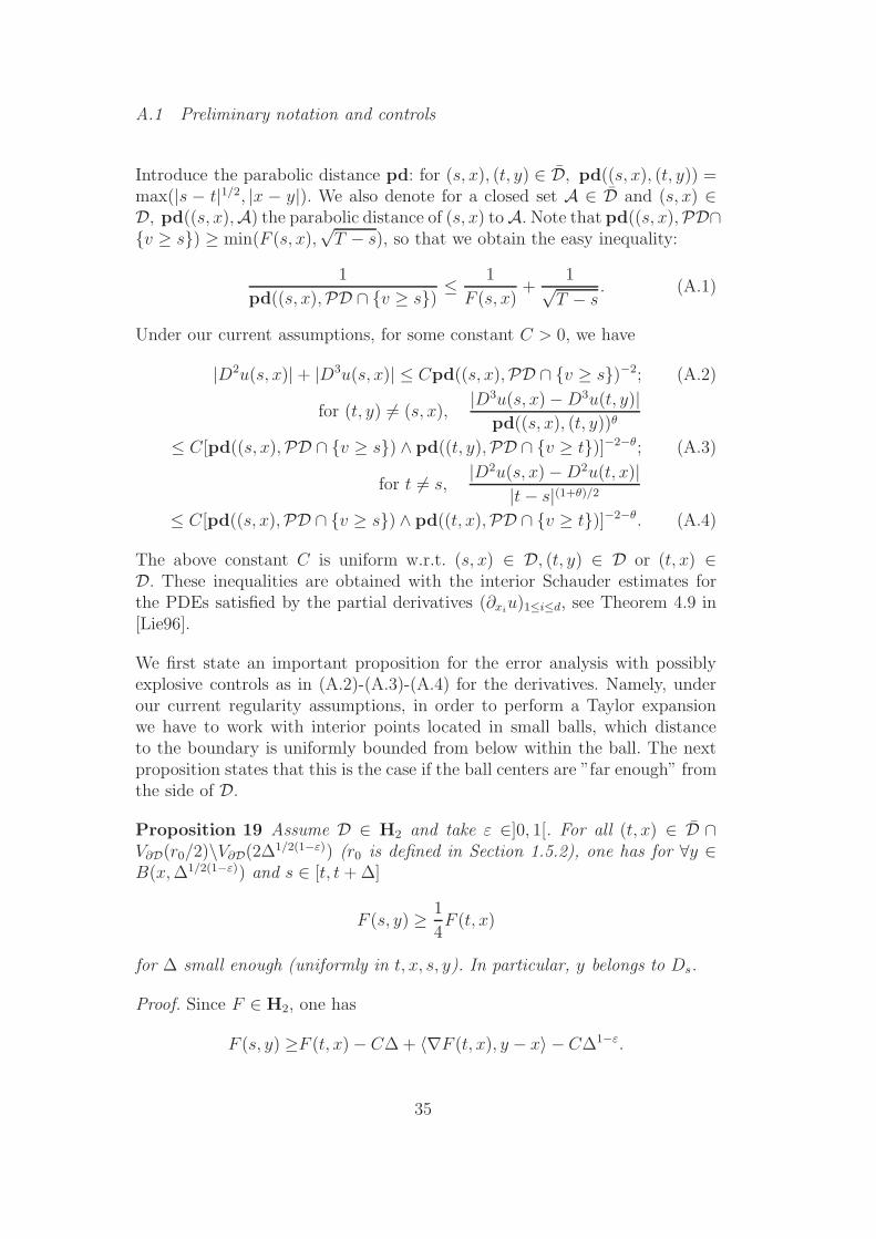
We first state an important proposition for the error analysis with possiblyexplosive controls as in (A.2)-(A.3)-(A.4) for the derivatives. Namely, underour current regularity assumptions, in order to perform a Taylor expansionwe have to work with interior points located in small balls, which distanceto the boundary is uniformly bounded from below within the ball. The nextproposition states that this is the case if the ball centers are ”far enough” fromthe side of D.

Proposition 19 Assume D ∈ H2 and take ε ∈]0, 1[. For all (t, x) ∈ D ∩V∂D(r0/2)\V∂D(2∆1/2(1−ε)) (r0 is defined in Section 1.5.2), one has for ∀y ∈B(x, ∆1/2(1−ε)) and s ∈ [t, t + ∆]

F (s, y) ≥ 1

4F (t, x)

for ∆ small enough (uniformly in t, x, s, y). In particular, y belongs to Ds.

Proof. Since F ∈ H2, one has

F (s, y) ≥F (t, x) − C∆ + 〈∇F (t, x), y − x〉 − C∆1−ε.

35

The norm of ∇F (t, x) equals 1, since ∇F (t, x) is the unit inward normalvector at the closest point of x on ∂Dt. Therefore, for ∆ small enough andusing 1

2F (t, x) ≥ ∆

12(1−ε), we have

F (s, y) ≥ F (t, x) − 3

2∆

12(1−ε) ≥ 1

4F (t, x),

which is the expected inequality. 2

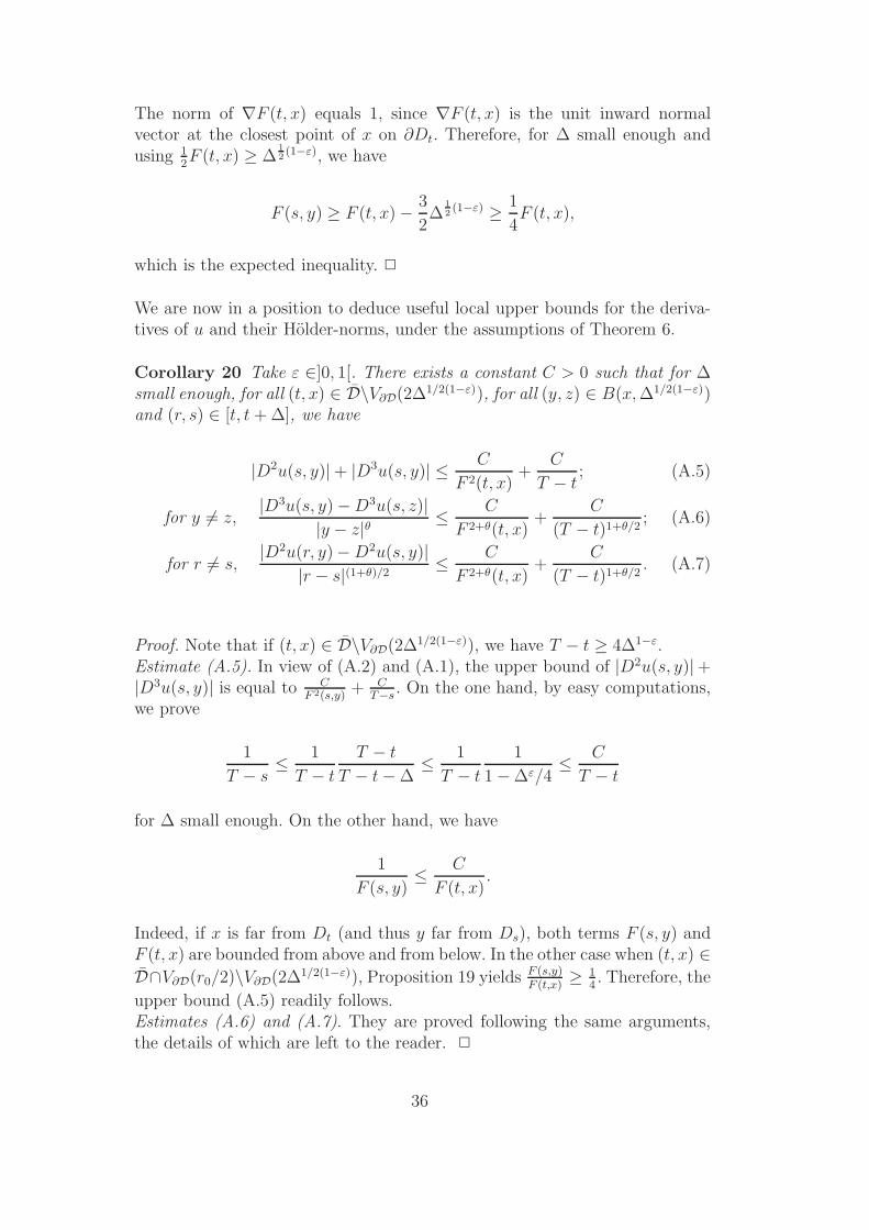
We are now in a position to deduce useful local upper bounds for the deriva-tives of u and their Holder-norms, under the assumptions of Theorem 6.

Corollary 20 Take ε ∈]0, 1[. There exists a constant C > 0 such that for ∆small enough, for all (t, x) ∈ D\V∂D(2∆1/2(1−ε)), for all (y, z) ∈ B(x, ∆1/2(1−ε))and (r, s) ∈ [t, t + ∆], we have

|D2u(s, y)|+ |D3u(s, y)| ≤ C

F 2(t, x)+

C

T − t; (A.5)

for y 6= z,|D3u(s, y) − D3u(s, z)|

|y − z|θ ≤ C

F 2+θ(t, x)+

C

(T − t)1+θ/2; (A.6)

for r 6= s,|D2u(r, y)− D2u(s, y)|

|r − s|(1+θ)/2≤ C

F 2+θ(t, x)+

C

(T − t)1+θ/2. (A.7)

Proof. Note that if (t, x) ∈ D\V∂D(2∆1/2(1−ε)), we have T − t ≥ 4∆1−ε.Estimate (A.5). In view of (A.2) and (A.1), the upper bound of |D2u(s, y)|+|D3u(s, y)| is equal to C

F 2(s,y)+ C

T−s. On the one hand, by easy computations,

we prove

1

T − s≤ 1

T − t

T − t

T − t − ∆≤ 1

T − t

1

1 − ∆ε/4≤ C

T − t

for ∆ small enough. On the other hand, we have

1

F (s, y)≤ C

F (t, x).

Indeed, if x is far from Dt (and thus y far from Ds), both terms F (s, y) andF (t, x) are bounded from above and from below. In the other case when (t, x) ∈D∩V∂D(r0/2)\V∂D(2∆1/2(1−ε)), Proposition 19 yields F (s,y)

F (t,x)≥ 1

4. Therefore, the

upper bound (A.5) readily follows.Estimates (A.6) and (A.7). They are proved following the same arguments,the details of which are left to the reader. 2

36

A.2 Error analysis

Recall from the previous proof of Theorem 6 that the main term to analyse is

e∆22

E=(

∑

0≤ti<T

1ti<τ∆1(Aεti

)C1∀s∈[ti,ti+1], X∆

s ∈B(X∆ti

,∆12 (1−ε))

[

u(ti+1, X∆ti+1

)Z∆ti+1

−u(ti, X∆ti

)Z∆ti

+ Z∆ti

f(ti, X∆ti

)∆])

1τr0>τ∆∧T

=(

∑

0≤ti<T−4∆1−ε

· · ·)

1τr0>τ∆∧T +(

∑

T−4∆1−ε≤ti<T

· · ·)

1τr0>τ∆∧T := e∆221 + e∆

222,

where we have just splitted the summation on ti.

Control of e∆221. The idea is to perform a stochastic expansion of u(ti+1, X

∆ti+1

)Z∆ti+1

−u(ti, X∆ti

)Z∆ti

+Z∆ti

f(ti, X∆ti

)∆ as in (2.8). Under our current assumptions, thedifference comes from the high-order derivatives that are no more uniformlybounded or uniformly Holder but only locally, with local estimates given inCorollary 20. Thus, following the same computations that have led to (2.10),we obtain

e∆221

E=(

∑

0≤ti<T−4∆1−ε

1ti<τ∆1(Aεti

)C1∀s∈[ti,ti+1], X∆s ∈B(X∆

ti,∆

12(1−ε))

[

O(

(∆2 + ∆|X∆s − X∆

ti|2)( 1

F 2(ti, X∆ti )

+1

T − ti))

+ O(

(∆1+ 1+θ2 + ∆|X∆

s − X∆ti|1+θ)(

1

F 2+θ(ti, X∆ti )

+1

(T − ti)1+θ/2))

+ Mti,ti+1

])

1τr0>τ∆∧T . (A.8)

The derivatives appearing in (Mti,ti+1)0≤ti<T (see equations (2.9) and (2.10))

are controlled by (A.5) on (Aεti)C . The control of (2.11) remains valid for the

(Mti,ti+1)0≤ti<T that yields a negligeable contribution. It follows that

|e∆221|

E

≤ C∆1+θ2

(

∑

0≤ti<T−4∆1−ε

1ti<τ∆1F (ti,X∆

ti)≥2∆

12(1−ε)∆

[

1

F 2+θ(ti, X∆ti )

+1

(T − ti)1+θ/2

])

1τr0>τ∆∧T .

Standard computations show that

∆1+θ2

∑

0≤ti<T−4∆1−ε

∆

(T − ti)1+θ/2≤ ∆

1+θ2

∫ T−4∆1−ε+∆

0

dt

(T − t)1+θ/2= O(∆

12+ θε

2 ),

which implies

|e∆221|

E

≤ C∆1+θ2

(

∫ T∧τ∆

01F (φ(t),X∆

φ(t))∈[2∆1/2(1−ε) ,r0/2]F (φ(t), X∆

φ(t))−2−θdt

)

+O(∆12+ θε

2 ).

37

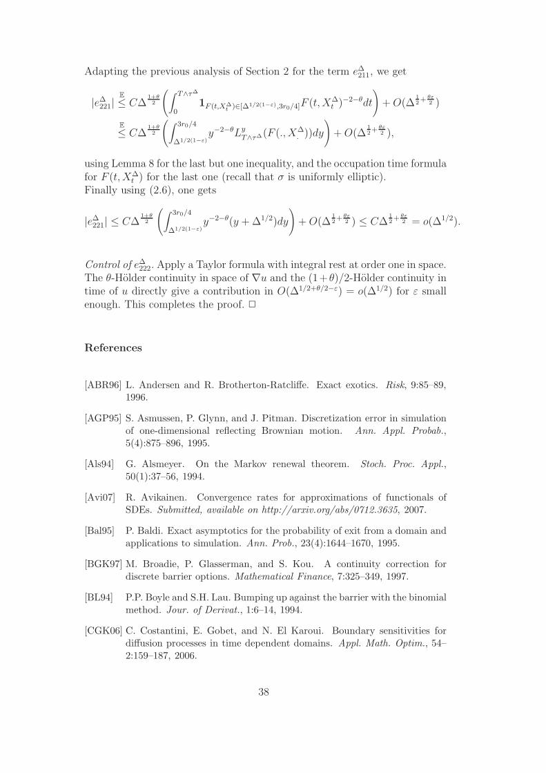
Adapting the previous analysis of Section 2 for the term e∆211, we get

|e∆221|

E

≤ C∆1+θ2

(

∫ T∧τ∆

01F (t,X∆

t )∈[∆1/2(1−ε),3r0/4]F (t, X∆t )−2−θdt

)

+ O(∆12+ θε

2 )

E

≤ C∆1+θ2

(

∫ 3r0/4

∆1/2(1−ε)y−2−θLy

T∧τ∆(F (., X∆. ))dy

)

+ O(∆12+ θε

2 ),

using Lemma 8 for the last but one inequality, and the occupation time formulafor F (t, X∆

t ) for the last one (recall that σ is uniformly elliptic).Finally using (2.6), one gets

|e∆221| ≤ C∆

1+θ2

(

∫ 3r0/4

∆1/2(1−ε)y−2−θ(y + ∆1/2)dy

)

+ O(∆12+ θε

2 ) ≤ C∆12+ θε

2 = o(∆1/2).

Control of e∆222. Apply a Taylor formula with integral rest at order one in space.

The θ-Holder continuity in space of ∇u and the (1+θ)/2-Holder continuity intime of u directly give a contribution in O(∆1/2+θ/2−ε) = o(∆1/2) for ε smallenough. This completes the proof. 2

References

[ABR96] L. Andersen and R. Brotherton-Ratcliffe. Exact exotics. Risk, 9:85–89,1996.

[AGP95] S. Asmussen, P. Glynn, and J. Pitman. Discretization error in simulationof one-dimensional reflecting Brownian motion. Ann. Appl. Probab.,5(4):875–896, 1995.

[Als94] G. Alsmeyer. On the Markov renewal theorem. Stoch. Proc. Appl.,50(1):37–56, 1994.

[Avi07] R. Avikainen. Convergence rates for approximations of functionals ofSDEs. Submitted, available on http://arxiv.org/abs/0712.3635, 2007.

[Bal95] P. Baldi. Exact asymptotics for the probability of exit from a domain andapplications to simulation. Ann. Prob., 23(4):1644–1670, 1995.

[BGK97] M. Broadie, P. Glasserman, and S. Kou. A continuity correction fordiscrete barrier options. Mathematical Finance, 7:325–349, 1997.

[BL94] P.P. Boyle and S.H. Lau. Bumping up against the barrier with the binomialmethod. Jour. of Derivat., 1:6–14, 1994.

[CGK06] C. Costantini, E. Gobet, and N. El Karoui. Boundary sensitivities fordiffusion processes in time dependent domains. Appl. Math. Optim., 54–2:159–187, 2006.

38

[DK06] R. A. Doney and A. E. Kyprianou. Overshoots and undershoots of Levyprocesses. Ann. Appl. Probab., 16–1:91–106, 2006.

[DL06] M. Deaconu and A. Lejay. A random walk on rectangles algorithm.Methodology And Computing In Applied Probability, 8(1):135–151, 2006.

[FL01] C.D. Fuh and T.L. Lai. Asymptotic expansions in multidimensionalMarkov renewal theory and first passage times for Markov random walks.Adv. in Appl. Probab., 33(3):652–673, 2001.

[Fre85] M. Freidlin. Functional integration and Partial differential equations.Annals of Mathematics studies, Princeton University Press, 1985.

[Fri64] A. Friedman. Partial differential equations of parabolic type. Prentice-Hall,1964.

[GM04] E. Gobet and S. Menozzi. Exact approximation rate of killed hypoellipticdiffusions using the discrete Euler scheme. Stoch. Proc. and Appl.,112:210–223, 2004.

[GM05] E. Gobet and S. Maire. Sequential Control Variates for Functionals ofMarkov Processes. Siam. Journal of Num. Analysis, 43-3:1256–1275, 2005.

[GM07] E. Gobet and S. Menozzi. Discrete sampling of functionals of Ito processes.Seminaire de Probabilites, XL:355–375, 2007.

[Gob00] E. Gobet. Euler schemes for the weak approximation of killed diffusion.Stoch. Proc. Appl., 87:167–197, 2000.

[Gob09] E. Gobet. Handbook of Numerical Analysis, Vol. XV, Special Volume:Mathematical Modeling and Numerical Methods in Finance, chapterAdvanced Monte Carlo methods for barrier and related exotic options,pages 497–528. Elsevier, Netherlands: North-Holland, 2009.

[GT98] D. Gilbarg and N.S. Trudinger. Elliptic partial differential equations ofsecond order. Springer Verlag, 1998.

[Lie96] G.M. Lieberman. Second Order parabolic differential equations, 1st edn.World Scientfic, River Edge, NJ, 1996.

[Men06] S. Menozzi. Improved simulation for the killed Brownian motion in a cone.Siam Jour. Num. Anal., 44-6:2610–2632, 2006.

[Mil97] G. N. Milstein. Weak approximation of a diffusion process in a boundeddomain. Stoch. Stoch. Reports, 64:211–233, 1997.

[MT99] G. N. Milstein and M. V. Tretyakov. Simulation of a space-time boundeddiffusion. Ann. Appl. Prob., 9–3:732–779, 1999.

[RY99] D. Revuz and M. Yor. Continuous martingales and Brownian motion.3rd ed. Grundlehren der Mathematischen Wissenschaften. 293. Berlin:Springer, 1999.

39

[Sie79] D. Siegmund. Corrected diffusion approximations in certain random walkproblems. Adv. in Appl. Probab., 11(4):701–719, 1979.

[Sie85] D. Siegmund. Sequential Analysis. Springer, 1985.

[Sim80] J Simon. Differentiation with respect to the domain in boundary valueproblems. Numer. Funct. Anal. Optim., 7–8:649–687, 1980.

[SY82] D. Siegmund and Y.S. Yuh. Brownian approximations for first passageprobabilities. Z. Wahrsch. verw. Gebiete, 59:239–248, 1982.

[TT90] D. Talay and L. Tubaro. Expansion of the global error for numericalschemes solving stochastic differential equations. Stoch. Anal. and App.,8-4:94–120, 1990.

[Woo82] M. Woodroofe. Nonlinear renewal theory in sequential analysis. SIAM,1982.

[Zha88] C.H. Zhang. A nonlinear renewal theory. Ann. Prob., 16-2:793–824, 1988.

40