Embed Size (px)
Citation preview

The American University in Cairo School of Sciences & Engineering
Mechanical Engineering Department
Sustainable Rural Community: Waste to Business (W2B) Model
By
Hala Omar
Dissertation submitted in partial fulfillment of the requirements of the degree of
Doctor of Philosophy in Engineering
with a concentration in
Mechanical Engineering
Under the supervision of:
Dr. Salah El-Haggar
Professor of Energy and Sustainable Development
Mechanical Engineering Department, The American University in Cairo
i
Abstract
Many environmental issues are facing rural villages in Egypt. The main problems rural
villages are suffering from are lack of adequate sewage system, absence of wastewater
treatment plants, poor agricultural and municipal solid waste management. These problems are
causing environmental, economic and social issues in rural villages. Rural communities’
residents suffer from many disease, unemployment as well as poor living conditions. It
becomes imperative to find solutions to this tragic situation facing rural villages associated
with dumping and burning waste. Unfortunately, not enough research is published to propose
solutions to approach full utilization of all types of wastes generated in rural villages and reach
sustainability.
The main goal of this research work is to develop and propose a concept to help rural
communities in Egypt approach full utilization of all types of wastes generated. This research
work is divided into three parts as follows: (1) developing a model to help rural villages in
Egypt reach full utilization of waste, (2) recycling of organic waste, (3) recycling of rejects.
In the first part of this research work desk research method is used. From the data
analysis it is proposed to use the concepts developed in industrial sector to reach sustainable
development such as the concept of cradle-to-cradle, industrial ecology, eco-industrial park,
environmental balanced industrial complex and green economy in the development of rural
villages. The concept of Waste to Business Model (W2B) is developed. It consists of
developing a facility in each rural village that groups simple and obtainable technologies in
one area to fully utilize all types of wastes generated from the rural village and transform it
into useful products.
The two following parts of this research work focus on two types of wastes that cause
huge problems in rural villages in Egypt which are: (1) organic waste and (2) rejects.
There are several types of organic waste and this research focuses on rice straw and
animal manure. It is estimated that around 2.5million tons/year of rice straw and 63milliom
ii
ton/year of animal manure are generated in Egypt. Composting process is and easy and cheap
solution to recycle organic waste. However, this method is not widely practiced in developing
countries because it is time consuming and the quality of product can be unstable. There have
been increasing attention on improving composting process. The aim of this part is to transform
rice straw into high quality soil amendments and organic fertilizer. This part is divided into
two sets of experiments. The objective of the first set of experiment is to transform rice straw
into soil amendment and evaluate the effect of different additives on the produced compost. In
the first set of experiment rice straw is inoculated with animal manure, Chinese starter,
cellulose decomposer and starter from the Egyptian Ministry of agriculture. The results of the
first set of experiments revealed that the application of different additives in composting of rice
straw exhibited an improvement of compost quality and results indicated that a higher
decomposition rate of treatment having animal manure, compared to other treatments.
Therefore, a second set of experiment has been conducted with substrate rice straw and animal
manure inoculated with different types of additives (Effective – micro-organisms, biochar,
Chinese starter) and mixture of natural rocks (rock phosphate, feldspar, sulfur, dolomite,
bentonite) to produce organic fertilizer. The results revealed that the application of different
additives in composting of rice straw exhibit an improvement in maturation time and final
product quality. The highest decomposition rate and highest organic fertilizer quality was
obtained in pile containing rice straw and 40% of animal manure mixed with natural rocks
(2.5% of rock phosphate, 2.5% feldspar, 2.5% sulfur, 2.5% dolomite and 10% bentonite) and
inoculated with 1L of activated EM and 10% biochar compared to other treatments. The pile
reached maturation after around 42 days. All analysis of the properties of the final product
indicated that it was in the range of the matured level and can be used without any limitation
as an organic fertilizer as it has met all the requirements by the Egyptian Specifications of
Organic fertilizers. The price of the produced high-quality organic fertilizer is 330LE/ton
iii
compared to chemical fertilizer market price ranging from 1,700LE/ton to 12,000LE/ton (non-
subsidized price). In addition to the direct cost, the use of chemical fertilizer damages the
atmosphere and the water. This damage has an unforeseen relatively high cost. Therefore,
organic fertilizer produced from organic waste can substitute expensive chemical fertilizer
The second major issue tackled in this research work is recycling of rejects. Rural
villages in Egypt suffer from poor recycling of the huge amount of MSW. Some types of MSW
can be easily recycled such as metals, glass, thermoplastics, etc., while others are perceived as
difficult or impossible to recycle. These un-recyclables are usually referred to as rejects. This
research focus on three types of rejects including (1) thermosets including melamine-
formaldehyde (a hard thermoset) and ethylene-propylene-diene- monomer rubber (EPDM
rubber an elastic thermoset), (2) multi-layer flexible packaging material, and (3) contaminated
plastic bags.
This part of the research work proposes two techniques to recycle rejects: (1) hot
technology and (2) a cold technology.
In the hot technology compression molding technique is used to produce the composite
material from waste multi-layer packaging material as the matrix and melamine-formaldehyde
as the filling material. In compression molding, the sample is subject to 50bar pressure and
heat for 30min. A full design of experiment is conducted to study the effect of the following
three factors on the property of the produced materials: (1) temperature, (2) %wt. of filling
material, and (3) particle size of filling material. For higher accuracy samples are produced at
random order using Design Expert software. The experimental results indicate that the highest
mechanical properties are obtained in samples produced using molding temperature of 145°C,
melamine-formaldehyde having a particle size of sieve 20 and 30%wt. fraction of melamine-
formaldehyde. The resulting product is found to be competitive to commercial MX and NX
types of Light Traffic Paving units in terms of cost and mechanical performance. In fact, the
iv
cost of produced material is 1.2LE/m2 compared to 150LE/m2 for interlock market price. Also,
substituting melamine-formaldehyde with other filling material like EPDM rubber waste or
sand and substituting the packaging material with contaminated plastic bags waste showed to
produce material slightly lower mechanical properties but can still be a competitive substitute
to produce interlocks.
In the second part, an innovative cold technology is proposed to produce cement bricks.
This technique consists of mixing contaminated plastic bags as coarse aggregates with sand,
marble powder and melamine-formaldehyde as fine aggregates with cement. The mix is then
pressed using a manual pressing machine without applying heat for few minutes to take the
shape of the mold. Then the brick is left to cure at ambient conditions and water is added every
day. The experimental results indicated that the highest properties are obtained after 28days of
curing in the mix made of 25%cement, 30% contaminated plastic bags, 15% sand, 15% marble
powder, 15% melamine-formaldehyde. The resulting product is found to be competitive to the
commercial non-load bearing masonry brick in terms of mechanical performance and cost. In
fact, the cost of produced material is 0.6LE/brick compared to 0.9 LE/brick for cement bricks.
The results of the research work indicate that applying the concept of W2B model in
rural villages will help these communities produce useful good that can substitute the use of
imported expensive products. Also, it will lead to creation of new job opportunities,
conservation of natural resources, and reduction of environmental and health problems related
to poor waste management.
v
List of Publications
• Omar, Hala, and Salah El-Haggar. "Zero Waste Rural Community Complex
(ZWRC2)." Environmental Management and Sustainable Development 6, no. 1 (2017):
105-118
• Omar, Hala, and Salah El-Haggar. "Sustainable Industrial Community. "Journal of
Environmental Protection 8, no. 03 (2017): 301-318.
• El-Haggar, Salah, and Hala Omar. “Sustainable and Cost-Effective use of Organic
Waste”. Current Trends in Biomedical Engineering & Biosciences 7, no. 4 (2017)
• Omar, Hala and Salah El-Haggar. “Proposed Sustainable Rural Community
Framework”. 4th International Conference on Sustainable Solid Waste Management,
Cyprus (2016)
• Omar, Hala contributor in chapters 7 and 9. Road Map for Global Sustainability: Rise
of The Green Communities”, by S.M. El-Haggar et. al., Advances in Science,
Technology & Innovation, IEREK Interdisciplinary series for Sustainable
Development, Springer Publisher House, 2019.
• Omar, Hala, Ibrahim, Yahia and El Haggar, Salah “Sustainable Bioconversion of Rice
Straw into High Quality Organic Fertilizer” submitted to Journal of Environmental
Protection
• Omar, Hala and Salah El Haggar, “Development of Innovative Cold Technology to
Produce Bricks from Rejects” in progress
vi
Acknowledgment
This dissertation would not have been possible without the guidance and help of many
people. First and foremost, I would like to express my utmost appreciation and gratitude to Dr.
Salah El-Haggar. I have been very privileged to get to know such a great and knowledgeable
Professor and to collaborate with him over the past years. He has always been patient and
encouraging in times of new ideas and difficulties. He was always promptly replying to my
frequent questions and ideas. The discussions with him often led to key insights. This research
work would not have been completed without his effort and time. Sparing the time during his
vacation to come to AUC to work with me was beyond expectation and is unforgettable and
extremely valued.
I am also indebted to Dr Yahia Ibrahim, assistant professor at the Soil Microbiology
Department, Soil, Water and Environment Research Institute, Agriculture Research Center. I
would like to thank Dr. Ibrahim for his contribution to the work done in Chapter 4 entitled.
“Sustainable Bioconversion of Agricultural Waste into High Quality Organic Fertilizer: Case
Study of Rice Straw”. He gave me the chance to get familiar with composting process and
helped in conducting all the testing at the Soil, Water and Environment Research Institute,
Agriculture Research Center. He was always orienting and supporting me with promptness and
care. His experience and knowledge in the field of organic fertilizer were of great importance
during this research.
I am also profoundly thankful to the staff of the Sustainable Development Laboratory,
Material Testing Laboratory and Construction Laboratory at AUC especially Mr. Mohamed
Said, Eng. Jaylan ElHalawani and Eng. Rasha Abdel Bary for offering me their generous
support throughout my research work.

vii
Nobody has been more important to me in the pursuit of this journey than the members
of my family. I would like to thank with all my heart my mum and dad. This journey could
have never been possible without their help, incessant support and guidance.
Last but not least, I would like to thank my husband for his continuous care and support,
encouragement and constant help. I could have never completed this work without his support.

viii
Dedication
I would like to dedicate this work to my children Youssef and Mariam for being my everlasting
source of love and inspiration.
ix
Table of Contents
Chapter 1 – Introduction ........................................................................................................ 1
1.1. Background ................................................................................................................ 1
1.2. Justification ................................................................................................................ 2
1.3. Research goal ............................................................................................................. 6
1.4. Structure of the dissertation ....................................................................................... 6
Chapter 2 – Literature Review ............................................................................................... 8
2.1. Main Problems facing rural communities in Egypt ................................................... 8
2.1.1. Huge amounts of organic waste ............................................................................... 10
2.1.2. Huge amounts of Municipal Solid Waste ................................................................ 13
2.1.3. Other important problems ........................................................................................ 16
2.2. Traditional Methods of Waste Disposal .................................................................. 17
2.3. Sustainability............................................................................................................ 18
2.3.1. From Cradle-to-Grave to Cradle-to-Cradle ............................................................. 19
2.3.2. Industrial Ecology (IE) and Eco-Industrial Park (EIP) ............................................ 21
2.3.3. Environmentally Balanced Industrial Complex (EBIC) .......................................... 22
2.3.4. Green Economy (GE) .............................................................................................. 22
2.3.5. Sustainable Development Goals .............................................................................. 23
2.4. Composting of organic waste ................................................................................... 23
2.4.1. Basic Concepts of Composting ................................................................................ 25
2.4.2. Composting of Rice Straw ....................................................................................... 27
2.4.3. Methods to improve composting process ................................................................ 28
2.5. Recycling of thermosets and packaging materials ................................................... 31
2.5.1. Recycling of thermosets ........................................................................................... 32
2.5.2. Recycling of food packaging materials .................................................................... 37
2.6. Summary of literature .............................................................................................. 41
2.7. Main Goal ................................................................................................................ 44
Chapter 3 – Waste to Business model (W2B) for sustainable rural communities ............ 45
3.1. Introduction .............................................................................................................. 45
3.2. Objectives ................................................................................................................ 45
3.3. Methodology ............................................................................................................ 46
3.4. Evaluation of the current waste management system in rural villages in Egypt ..... 48
3.4.1. Major Waste composition in Egypt .................................................................. 48
3.4.2. Current practices of waste management in rural villages in Egypt ................ 49
3.4.3. Problems associated with waste management in rural villages in Egypt ........ 50
3.5. Pathway to Sustainable Rural Communities in Egypt ............................................. 51
3.5.1. Sustainable Strategies in industrial sector ...................................................... 51
x
3.5.2. Plans and strategies for waste management in Egypt ..................................... 52
3.6. Proposed Waste to Business Model (W2B) for Rural Communities ....................... 54
3.7. Conclusion ............................................................................................................... 60
Chapter 4 – Sustainable bio-conversion of AGRICULTURAL WASTE into high quality
organic fertilizer – CASE STUDY OF RICE STRAW ...................................................... 63
4.1. Objectives ................................................................................................................ 65
4.2. Materials and Methods ............................................................................................. 65
4.1.1. Raw Material ................................................................................................... 66
4.1.2. Organic additives ............................................................................................. 66
4.1.3. Composting procedure ..................................................................................... 68
4.1.4. Measured Parameters ...................................................................................... 70
4.1.5. Statistical Analysis ........................................................................................... 73
4.3. Results and discussion ............................................................................................. 73
4.3.1. Bioconversion of organic waste into soil amendment ..................................... 73
4.3.2. Bioconversion of organic waste into high quality organic fertilizer ............... 92
4.4. From organic waste to sustainable green business opportunity in rural Egypt ...... 115
4.5. Conclusion ............................................................................................................. 128
Chapter 5– APPROACHING FULL UTILIZATION OF MUNICIPAL SOLID WASTE
– CASE STUDY OF REJECTS .......................................................................................... 130
5.1. Introduction ............................................................................................................ 130
5.2. Objectives .............................................................................................................. 132
5.3. Development of an innovative composite material to produce interlock paving units
from rejects using hot technology ...................................................................................... 134
5.3.1. Methodology .................................................................................................. 134
5.3.2. Measured Properties ...................................................................................... 139
5.3.3. Results and discussion ................................................................................... 146
5.3.4. Possible Application ...................................................................................... 168
5.3.5. Cost Analysis .................................................................................................. 175
5.3.6. Conclusion ..................................................................................................... 176
5.4. Development of innovative cold technology to produce bricks from rejects ........ 177
4.5.1. Methodology .................................................................................................. 177
4.5.2. Measured Properties ...................................................................................... 182
4.5.3. Results and Discussion .................................................................................. 184
4.5.4. Cost Analysis .................................................................................................. 191
4.5.5. Conclusion ..................................................................................................... 192
5.5. Conclusion ............................................................................................................. 193
Chapter 6– conclusion and recommendations .................................................................. 194
xi
6.1. Conclusions ............................................................................................................ 194
6.1.1. Waste to business Model for Sustainable Rural Communities ...................... 194
6.1.2. Sustainable bio-conversion of agricultural waste into high quality organic
fertilizer: case study of rice straw .................................................................................. 196
6.1.3. Approaching full utilization of Municipal Solid Waste: case study of rejects
198
6.1.4. Closing the loop and clearing the path towards sustainable rural communities
201
6.2. Recommendations .................................................................................................. 204
6.2.1. Sustainable bio-conversion of agricultural waste into high quality organic
fertilizer: case study of rice straw .................................................................................. 204
6.2.2. Approaching full utilization of Municipal Solid Waste: case study of rejects
204
References ............................................................................................................................. 206
Appendix ............................................................................................................................... 220
xii
List of Figures
Figure 2.1: Sources of Organic Waste in Egypt ...................................................................... 11
Figure 2.2: Burning Agricultural Waste in field in rural Egypt [32] ....................................... 12
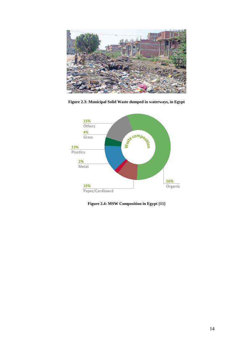
Figure 2.3: Municipal Solid Waste dumped in waterways, in Egypt ...................................... 14
Figure 2.4: MSW Composition in Egypt [11] ......................................................................... 14
Figure 2.5 - Cradle- to- Grave Approach [43] ......................................................................... 20
Figure 2.6 – Cradle-to-Cradle Approach [43].......................................................................... 21
Figure 2.7 – Summary of composting process [28] ................................................................. 24
Figure 2.8: Phases of the composting process [56].................................................................. 25
Figure 3.1: Major waste constituents in Egypt ........................................................................ 49
Figure 3.2: Pathway to Sustainable Rural Community in Egypt ............................................. 53
Figure 3.3: Waste to Business Model for Sustainable Rural Communities ............................. 55
Figure 3.4: Summary of the Research Sequence ..................................................................... 62
Figure 4.1: Summary of composting process .......................................................................... 70
Figure 4.2: Changes in temperatures in compost piles with relation to ambient temperatures
for (a) E1.T1, (b) E1.T2, (c) E1.T3, (d) E1.T4 and (e) E1.T5 ................................................. 76
Figure 4.3: Changes in %organic matter in different compost treatments in set of experiment
# 1............................................................................................................................................. 78
Figure 4.4: Changes in %organic carbon in different compost treatments in set of experiment
# 1............................................................................................................................................. 78
Figure 4.5: Percentage losses in organic matter and organic carbon in different compost
treatments in set of experiment # 1 .......................................................................................... 79
Figure 4.6: Total Nitrogen in different compost treatments in set of experiment # 1 ............. 80
Figure 4.7: Ammonium Nitrogen in different compost treatments in set of experiment # 1 .. 81
Figure 4.8: Nitrate Nitrogen in different compost treatments in set of experiment # 1 ........... 82
Figure 4.9: C/N ratio in different compost treatments in set of experiment # 1 ...................... 84
Figure 4.10: Moisture Content in different compost treatments in set of experiment # 1 ....... 85
Figure 4.11: Bulk density in different compost treatments in set of experiment # 1 ............... 85
Figure 4.12: Electrical Conductivity in different compost treatments in set of experiment # 1
.................................................................................................................................................. 86
xiii
Figure 4.13: pH in different compost treatments in set of experiment # 1 .............................. 87
Figure 4.14: Total Phosphorous in different compost treatments in set of experiment # 1 ..... 90
Figure 4.15: Total Potassium in different compost treatments in set of experiment # 1 ......... 91
Figure 4.16: Changes in temperatures in compost piles with relation to ambient temperatures
for (a) E2.T1, (b) E2.T2, (c) E2.T3, (d) E2.T4, (e) E2. T5, (f) E2.T6, (g) E2.T7, (h) E2.T8, (i)
E2.T9 ........................................................................................................................................ 96
Figure 4.17: Changes in %organic matter in different compost treatments in set of experiment
# 2............................................................................................................................................. 98
Figure 4.18: Changes in %organic carbon in different compost treatments in set of
experiment # 2.......................................................................................................................... 99
Figure 4.19: Percentage losses in organic matter and organic carbon in different compost
treatments in set of experiment # 2 ........................................................................................ 100
Figure 4.20: Total Nitrogen in different compost treatments in set of experiment # 2 ......... 101
Figure 4.21: Ammonium Nitrogen in different compost treatments in set of experiment # 2
................................................................................................................................................ 102
Figure 4.22: Nitrate Nitrogen in different compost treatments in set of experiment # 2 ....... 102
Figure 4.23: C/N ratio in different compost treatments in set of experiment # 2 .................. 104
Figure 4.24: Moisture Content in different compost treatments in set of experiment # 2 ..... 105
Figure 4.25: Bulk density in different compost treatments in set of experiment # 2 ............. 106
Figure 4.26: Electrical Conductivity in different compost treatments in set of experiment # 2
................................................................................................................................................ 107
Figure 4.27: pH in different compost treatments in set of experiment # 2 ............................ 107
Figure 4.28: Total Phosphorous in different compost treatments in set of experiment # 2 ... 112
Figure 4.29: Total Potassium in different compost treatments in set of experiment # 2 ....... 113
Figure 4.30: Physical appearance of E2.T6 (a) at the beginning of compost process, after (b)
30 days, (c) 60 days, and (c) 90 days ..................................................................................... 114
Figure 5.1: Preparation of waste material .............................................................................. 135
Figure 5.2: Mixer ................................................................................................................... 136
Figure 5.3: Compression Molding machine........................................................................... 136
Figure 5.4: Schematic diagram for recycling of rejects using hot technology ...................... 138
Figure 5.5: Compressive strength test apparatus ................................................................... 139
xiv
Figure 5.6: Abrasion test apparatus ....................................................................................... 140
Figure 5.7: Flexural strength test apparatus ........................................................................... 142
Figure 5.8: Digital pH meter .................................................................................................. 143
Figure 5.9: TSS measuring devices (a) digital balance, (b)filter paper, (c) oven .................. 143
Figure 5.10: TDS meter ......................................................................................................... 144
Figure 5.11: Nitrate spectrophotometer ................................................................................. 144
Figure 5.12: (a) water samples with reagent, (b) COD reactor, (c) Spectrophotometer ........ 145
Figure 5.13: Atomic absorption spectrometer to measure heavy metals ............................... 145
Figure 5.14: Model Adequacy checking for compressive strength response (a) normal
probability plot, (b) Residuals versus predicted plots and (c) Residuals versus runs ............ 148
Figure 5.15: 3D plot for compressive strength response at (a) sieve 16, (b) sieve 20 and (c)
sieve 40 .................................................................................................................................. 149
Figure 5.16: Model Adequacy checking for density response (a) normal probability plot, (b)
Residuals versus predicted plots and (c) Residuals versus runs ............................................ 153
Figure 5.17: Model Adequacy checking for water absorption response (a) normal probability
plot, (b) Residuals versus predicted plots and (c) Residuals versus runs .............................. 156
Figure 5.18: Model Adequacy checking for flexural strength response (a) normal probability
plot, (b) Residuals versus predicted plots and (c) Residuals versus runs .............................. 160
Figure 5.19: 3D plot for flexural strength response at (a) sieve 16, (b) sieve 20 and (c) sieve
40............................................................................................................................................ 162
Figure 5.20: Water samples of (a) three replicates of 17M, (b) packaging material, (c)
melamine formaldehyde......................................................................................................... 166
Figure 5.21: Compressive Strength of MP – MF composite material ................................... 172
Figure 5.22: Water absorption of MP – MF composite material ........................................... 173
Figure 5.23: Abrasion Index of MP – MF composite material .............................................. 174
Figure 5. 24: Summary of recycling of rejects using cold technology .................................. 181
Figure 5.25: Compression Machine ....................................................................................... 183
Figure 5.26: Water Absorption test ........................................................................................ 184
Figure 5.27: Compressive Strength of produced bricks after 7, 14 and 28 days ................... 189
Figure 6.1: Complete Waste to Business Model (W2B) ........................................................ 203

xv
List of tables
Table 2.1: Average quantity of some agricultural residues in rural Egypt from 2011 to 2013
[12]: .......................................................................................................................................... 11
Table 2.2: Daily generated MSW in some governorates in Egypt in 2012 [11]:..................... 15
Table 4.1: Properties of rice straw ........................................................................................... 66
Table 4.2: Piles content used for composting process in set of experiment # 1 ...................... 68
Table 4.3: Piles content used for composting process in set of experiment # 2 ...................... 69
Table 4.4: Types of rocks used and their corresponding quantities ......................................... 69
Table 4.5: Summary of measured parameters.......................................................................... 72
Table 4.6: NH4/NO3 for different treatments in set of experiment # 1 ................................... 82
Table 4.7: Germination Index and humification index for different treatments in set of
experiment # 1 after 90 days of composting ............................................................................ 88
Table 4.8: Pathogenic bacteria for different treatments in set of experiment # 1 .................... 89
Table 4.9: NH4/NO3 for different treatments in set of experiment # 2 ................................. 103
Table 4.10: Germination Index and humification index for different treatments in set of
experiment # 2 after 90 days of composting .......................................................................... 109
Table 4.11 Pathogenic bacteria for different treatments in set of experiment # 2 ................. 110
Table 4.12: Demand and Supply of chemical fertilizer in Egypt [184] ................................. 116
Table 4.13: Price of raw material used in composting high quality organic fertilizer........... 121
Table 4.14: Comparison of price of organic and chemical fertilizer ..................................... 124
Table 4.15: Comparison of price of organic and chemical fertilizer [192] ........................... 126
Table 5.1: Compressive strength of MP + MF composite material ....................................... 146
Table 5.2: ANOVA table for compressive strength response............................................... 148
Table 5.3: Compressive Strength Response model fit statistics ............................................ 151
Table 5.4: Densities of MP + MF composite material ........................................................... 152
Table 5.5: ANOVA table for Density response ..................................................................... 154
Table 5.6: Water absorption of MP + MF composite material .............................................. 155
Table 5.7: ANOVA table for water absorption ...................................................................... 157
Table 5.8: Flexural Strength of MP – MF composite material .............................................. 159
Table 5.9: ANOVA table for flexural strength response ....................................................... 161
xvi
Table 5.10: Abrasion of MP + MF composite material ......................................................... 164
Table 5.11: Abrasion Index of MP + MF composite material ............................................... 165
Table 5.12: Water Analysis results ........................................................................................ 166
Table 5.13: Summary of the mechanical properties of the three produced composite materials
................................................................................................................................................ 168
Table 5.14: Properties of Light Traffic Paving Units based on ASTM C902 ....................... 170
Table 5.15: Abrasion index of Light Traffic Paving Units based on ASTM C902 ............... 170
Table 5.16: Cost calculation and comparison with commercial prices ................................. 175
Table 5.17: Particle gradation by mass .................................................................................. 179
Table 5.18: Mixes used in cold technology ........................................................................... 180
Table 5.19: Compressive strength of different bricks ............................................................ 185
Table 5.20: One Way ANOVA for Compressive Strength.................................................... 186
Table 5.21: Tukey’s HSD test for Compressive Strength...................................................... 188
Table 5.22: Compression Strength (MPa) for non-load bearing concrete masonry units ..... 189
Table 5.23: Water absorption of produced bricks .................................................................. 190
Table 5.24: Density of produced bricks ................................................................................. 191
Table 5.25: Standard requirement of oven dry density of concrete ....................................... 191
Table 5.26: Cost calculation and comparison with commercial prices for cold technology . 191
xvii
List of Abbreviations
ANOVA Analysis of variance
ASTM American Society for Testing Material
CAPMAS Central Agency for Public Mobilization and Statistics
C2C Cradle to Cradle
C2G Cradle to Grave
Cd Cadmium
C/N ratio Carbon to Nitrogen ratio
COD Chemical Oxygen Demand
Cr Chromium
EBIC Environmentally Balanced Industrial Complex
EC Electric conductivity
EIP Eco-Industrial Park
EM Effective Micro-organisms
EPA United States Environmental Protection Agency
EPDM Ethylene-Propylene-Diene Monomer
GI Germination Index
HI Humification Index
IE Industrial Ecology
MF Melamine-formaldehyde
MP Multilayer packaging material
MSW Municipal Solid Waste
NH3- Nitrate Nitrogen
NH4+ Ammonia nitrogen
OC Organic Carbon
OM Organic Matter
PB Plastic bags
Pb Lead
SDG Sustainable Development Goals
TDS Total Dissolved Solids
TK Total Phosphorous
TN Total Nitrogen
TP Total Potassium
TSS Total Suspended Solids
W2B Model Waste to Business Model
1
CHAPTER 1 – INTRODUCTION
1.1. Background
Egypt is making many progress in many fields; yet, millions of individuals are still
living in extreme poverty in rural areas. According to Central Agency for Public Mobilization
and Statistics (CAPMAS) [1], 57.4% of the Egyptian population lives in rural areas in 2018.
Also, CAPMAS income and expenditures survey for the year 2015 [2] revealed that 27.5% of
the Egyptian population is under the national poverty line (poverty line is LE 485 per month).
The poverty rate in Cairo is 17.5%, while the poverty rate in rural areas varies from 13.1% to
66% [2]. Of course, not all villages are equally poor, smaller and more remote villages called
satellites or affiliated villages tend to be poorer than larger and less remote ones, known as
mother villages.
In these rural areas, people live in miserable conditions. They do not have adequate
dwelling, they suffer from illiteracy, unemployment, they are at high risk for disease and suffer
from high mortality rate and low life expectancy [3, 4, 5, 6]. To solve their problems people
living in rural areas look for cheap and easy solutions to their problems. They informally build
their own houses and drainage system as well as use electricity connections from adjacent
houses. However, these solutions most often result into environmental problems including
spreading of substandard housing, poor sewage system, poor environmental sanitation, etc.
They also suffer from unemployment or work in irregular and low paid-jobs. Many people do
not tolerate theses harsh living conditions and are forced to leave their home villages and move
to the capital.
The rampant urban growth has widened urban-rural disparities. These challenges are
ignored by governments, entrepreneurs, environmentalists and society and pretend that these
areas do not have any impact on urban prosperity. Yet, the growth of slums and informal
settlements in urban areas is strongly related to the urban-rural disparities. It became urgent to
2
propose innovative solutions to help ameliorate the quality of life of millions of residents of
rural villages.
1.2. Justification
Rural communities in Egypt are confronted with many environmental issues due to the
huge amount of waste generated every year including municipal solid waste (such as metals,
glass, plastics, rejects, ...), wastewater, organic waste (such as agricultural waste and animal
manure, ...) etc. These wastes are poorly disposed of and managed causing serious problems
and burden to the country, while they could be hidden treasures if used optimally. These
problems are causing environmental, economic and social issues in rural villages Rural
communities’ residents suffer from many disease, unemployment as well as poor living
conditions [4, 7, 8]. It becomes imperative to find solutions to the environmental, economic
and social tragic situation facing rural villages associated with dumping and burning waste.
Many efforts have been made since the emergence of the concept of sustainable development
to reach zero-pollution. To address the problems of depletion of natural resources and
environmental problems caused by human activities the concepts of cradle-to-cradle have been
developed to fully utilize industrial waste. Not enough research is published to propose
solutions to approach full utilization of all types of wastes generated in rural villages and reach
sustainability.
The Egyptian Government as well as the United Nations have defined Sustainable
Development Goals (SDGs) for 2030 to help the country develop a clean, safe and healthy
environment leading to improved economic situation, providing new job opportunities and
reducing poverty [9, 10]. Therefore, the main goal of this research work is to aid rural
communities reach zero-pollution via sustainable and affordable methods to contribute to the
SDGs. In order to reach these goals, the Waste to Business Model (W2B) for rural communities
3
is developed and proposed in this research work as a solution to help rural villages reach 100%
full utilization of all types of wastes.
While studying the different waste streams generated in rural areas in Egypt, it became
obvious that one of the utmost important problems facing rural villages in Egypt is the huge
amount of organic waste that represents around 133million tons/year [11]. There are several
types of organic waste and this research focuses on agricultural waste as a type of organic
waste. Egypt generates up to 30 million ton/year of agricultural waste [12], from which 52%
are directly burnt in the fields [13]. The lack of environmental awareness of farmers coupled
with poor farmers skills and knowledge in managing agriculture waste [14] and high cost of
traditional disposal methods causes farmers to burn their waste in the field [5]. This causes
depletion of natural resources as well as pollution of the environment. One of the main types
of agricultural waste generated in Egypt is rice straw [15]. It is estimated that about 3.1million
tons per year of rice straw are disposed of by directly burning in open fields causing serious
environmental problems, including air pollution and soil degradation due to lack of cost-
effective treatment approaches [16, 17]. Composting process is considered one of the most
suitable alternatives to manage and treat organic waste to produce soil amendments and organic
fertilizers [18, 19, 20]. However, this method is not widely practiced in developing countries
because it is time consuming and quality of product received can be unstable [11, 21]. Hence,
many studies reported methods to improve composting process including co-composting with
animal manure as well as inoculation of compost piles with microbial additives or biochar to
accelerate the composting process and increase the nutritional values of produced soil
amendment or organic fertilizer. Yet, there are still knowledge gaps to fully understand the
composting process due to the variety of feedstock. Therefore, the second aim of this research
is to study and compare the effect of co-composting with animal manure, inoculation of
4
compost piles with different commercially available microbial additives and biochar on the
composting process of rice straw.
Another serious problem rural villages suffer from is poor municipal solid waste
(MSW) management. According to the country report on the solid waste management in Egypt
prepared by the Regional Solid Waste Exchange of Information and Expertise Network in
Mashreq and Maghreb Countries (SWEEP-Net) in 2014 [11], Egypt generates 21million tons
of MSW per year. Only 65% of the generated waste is collected and properly disposed of or
recycled [11]. The rest either accumulates in streets, waterways, drains and/or illegal dumping
sites causing many environmental and health problems [5, 6, 22]. In order to adequately
manage municipal solid waste, it is also crucial to raise awareness of people and develop simple
and cheap technologies to recycle waste.
A large amount of waste generated in Egypt is made out of unrecyclable waste known as rejects
[5]. There are many types of rejects and this research focuses on three types of rejects: (1)
thermosets, (2) packaging materials, and (3) contaminated plastic bags.
Thermoset is a type of plastic that have many attractive properties (high hardness,
thermal resistance, insulation, etc.), which make it significantly used in many applications. All
of these properties are attributed to the complex three-dimensional structure of the material.
Yet, this cross-linked nature makes thermosets very challenging to recycle as they decompose
and degrade when subject to heat. Therefore, most of the thermoset products end up in landfills
or are incinerated at the end of their life, which causes serious environmental concerns due to
the fact that plastic waste contains various toxic elements, which can pollute soil and water
[23, 24]. Due to the increasing environmental concern, recycling of non-biodegradable
thermoset wastes has been the major issue for researchers [25].
Another type of reject is packaging materials. Packaging material could be made of
paper and cardboard, glass, aluminum, plastics or laminated packaging material. The laminated
5
packaging material are usually the ones referred to as rejects as they are hard to recycle because
they are made of multilayer films of different materials bonded together. The Central
Department of Solid Waste estimate that around 29% of MSW in Egypt could be made of
packaging materials, which represents 6 million tons [11]. Very limited number of publications
reported the mechanical recycling of multi-layer flexible packaging material to produce useful
goods. Most of literature focus on expensive and energy consuming recycling techniques, such
as thermal-chemical methods, microwave induces pyrolysis or plasma technology to separate
the layers and recover each material separately, which makes them not implemented and
introduced in poor developing countries.
The third type of rejects is single-use garbage plastic bags usually made of low-density
polyethylene (LDPE). They cause a huge threat to the environment as they are non-
biodegradable. It is estimated that 5 trillion bags are produced worldwide every year [26].There
is no published data about the exact amount of garbage plastic bags consumed; however, the
head of the Environmental Affairs Agency, Shehab Abdel Wahab stated in an interview with
Egypt today online journal that around 12 billion waste plastic bags are generated each year
[27]. Plastic bags are also often burned, releasing toxic fumes into the air causing
environmental problems. Hence, the Egyptian Ministry of Environment launched the EU-
funded initiative called “Enough Plastic Bags” in 2017, aiming to reduce their use due to the
negative effects on the environment and the economy. Yet, the current huge amounts of plastic
bags produced needs to be recycled. Very few number of publications reported the mechanical
properties of products recycled from garbage plastic bags [28].
Therefore, the third aim of this research is to develop easy and cheap technology to
recycle rejects to produce useful goods for rural community. This part of the research will focus
on recycling of melamine- formaldehyde (a hard thermoset), ethylene-propylene-diene-
6
monomer rubber (an elastic thermoset), multi-layer flexible packaging material and garbage
plastic bags.
1.3. Research goal
The main goal of this research work is to find innovative means to ameliorate the quality
of life in rural villages and develop Sustainable Rural Communities and reach zero-pollution
via sustainable and affordable methods.
n order to achieve this main goal, this research work is divided into three parts having the
following aims:
1. To develop a concept/model to help rural villages reach 100% full utilization of all
types of wastes.
2. To produce high quality organic fertilizer from organic waste generated in rural areas
to substitute expensive chemical fertilizers currently used
3. To produce new composite materials from rejects generated in rural areas and make
useful goods
1.4. Structure of the dissertation
Chapter 1 is the introduction to this research work; it contains background information
and presents problems facing rural areas in Egypt and finally introduced the main goals of the
research. This chapter is followed by the literature review (Chapter 2) that presents data
collected and found in books, journal papers, conference papers, governmental reports,
international organizations’ statistics and websites concerning the main environmental
problems facing rural areas in Egypt, the traditional waste disposal methods, the sustainability
concepts, composting of organic waste and recycling of rejects. Afterwards, the three parts of
this research work are presented, consecutively as follows:
7
Chapter 3 is entitled “Waste to Business Model (W2B) for Sustainable Rural
Communities”. In this chapter the developed concept of W2B is fully described.
Chapter 4 is entitled “Sustainable Bio-conversion of Agricultural Waste into High
Quality Organic Fertilizer: Case Study of Rice Straw”. In this chapter the effect of
different additives, including biochar, effective micro-organisms (EM), animal manure
and commercial microbial inoculants, on the bioconversion of rice straw is investigated.
Two sets of experiments are described. The aim of the first set of experiment is to
produce high quality soil amendment and the aim of the second set of experiment is to
produce high quality organic fertilizer. The used materials and bioconversion method
are fully explained, and the results and discussions are thoroughly presented. The cost
of the produced organic fertilizer is compared with the price of commercially available
chemical fertilizer.
Chapter 5 is entitled “Approaching Full Utilization of Municipal Solid Waste: Case
Study of Rejects”. In this chapter two innovative technologies and products are
proposed to recycle rejects (packaging material, melamine formaldehyde, EPDM
rubber and garbage plastic bags) to produce interlock paving units and bricks. The
mechanical properties of the produced composite material are fully presented. The costs
of the produced materials are compared with price of commercially available products
having comparable properties.
These three chapters presents the objectives methodology, and results and discussion for each
topic.
The conclusion and recommendations are finally presented in chapter 6.
8
CHAPTER 2 – LITERATURE REVIEW1
This literature review discusses thoroughly the major environmental problems related
to poor waste management facing rural communities in Egypt as well as their impact on
different aspects of life. The major reason behind poor waste management is that the cost of
traditional methods of waste disposal is exponentially escalating and this cause a huge financial
burden for poor rural communities’ residents. On the other hand, finding new sources of raw
material is becoming costly and difficult. Therefore, the advantages and disadvantages of
traditional disposal methods used in rural Egypt are fully presented as well. This research
focuses on implementing concept of sustainability in rural context and then two major
problems facing rural communities are tackled in depth:
Recycling of Organic waste as one of the utmost important problems facing rural
villages in Egypt is the huge amount of organic waste generated every year, and
Recycling of Rejects as large amount of rejects; such as packaging material, thermosets,
contaminated plastic bags, are generated every year and accumulates in streets, water
canals and/or illegal dumpsites as they are very challenging to recycle.
Hence, state-of-the art methods found in the literature for composting of organic waste as well
as recycling of rejects are fully presented.
2.1. Main Problems facing rural communities in Egypt
Egypt is a major actor in the Middle East and North Africa. It has the largest and most
densely settled population among the Arab countries. It is divided into twenty-seven
governorates that can be divided as follows [3, 29, 30]:
1 Part of the work in this chapter was published in a review papers by Omar, Hala and El-Haggar, Salah entitled
“Sustainable Industrial Community” [43] as well as in chapter 9 of a book entitled “Road Map for Global
Sustainability: Rise of The Green Communities”, by S.M. El-Haggar et. al., Advances in Science, Technology &
Innovation, IEREK Interdisciplinary series for Sustainable Development, Springer Publisher House, 2019 [28].
9
Urban governorates: Cairo, Alexandria, Port Said and Suez, that have no rural
population
Lower Egypt: having nine governorates subdivided into urban and rural areas
o Behera
o Dakahlia
o Gharbia
o Menoufia
o Kalyoubia
o Ismailia
o Sharkia
o Damietta
o Kafr El-Sheikh
Upper Egypt: having eight governorates subdivided into urban and rural areas
o Fayoum
o Giza
o Menia
o Luxor
o Aswan
o Asyiut
o Beni-Suef
o Qena
o Suhaj
Frontier Governorates located on eastern and western boundaries of Egypt
o Red Sea
o New Valley
10
o South Sinai
o Matruh
o North Sinai
Egypt population is increasing dramatically. According to the Central Agency for
Public Mobilization and Statistics (CAPMAS), the Egyptian population has increased from
72million people in 2006 to 97 million people in 2018 [31, 1]. According to Central Agency
for Public Mobilization and Statistics (CAPMAS) [1], 57.4% of the Egyptian population lives
in rural areas in 2018. Based on Nassar and Biltagy [4], most of the country’s poor people live
in rural Upper Egypt. In fact, out of the 1000 poorest villages in Egypt 941 are located in Upper
Egypt [4]. Upper Egypt is home to about 40% of the Egyptian population and contains 60% of
the poor [29]. Of course, not all villages are equally poor, smaller and more remote villages
called satellite or affiliated villages tend to be poorer than larger and less remote ones, known
as mother villages. According to Nassar and Biltagy [4], Qena governorate suffers from
poverty most severely from among all Upper Egypt.
The absence of adequate sewage system, lack of agricultural and municipal solid waste
management makes residents of rural areas in Egypt live in squalid areas. They burn their waste
in the field or throw them in the streets and/or in the nearest water way. These practices cause
air, soil and water pollution. These people also suffer from social and economic problems
including diseases, high mortality rate, low life expectancy, illiteracy and unemployment [28].
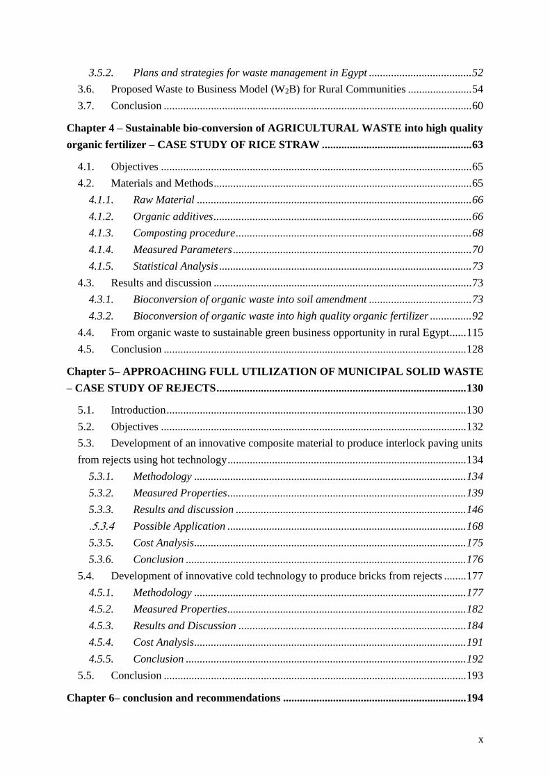
2.1.1. Huge amounts of organic waste
One of the utmost important problems facing rural villages in Egypt is the huge amount
of organic waste. There are several types of organic waste including organic waste from
municipal solid waste (MSW), agricultural waste, animal manure, sewage, and waterway
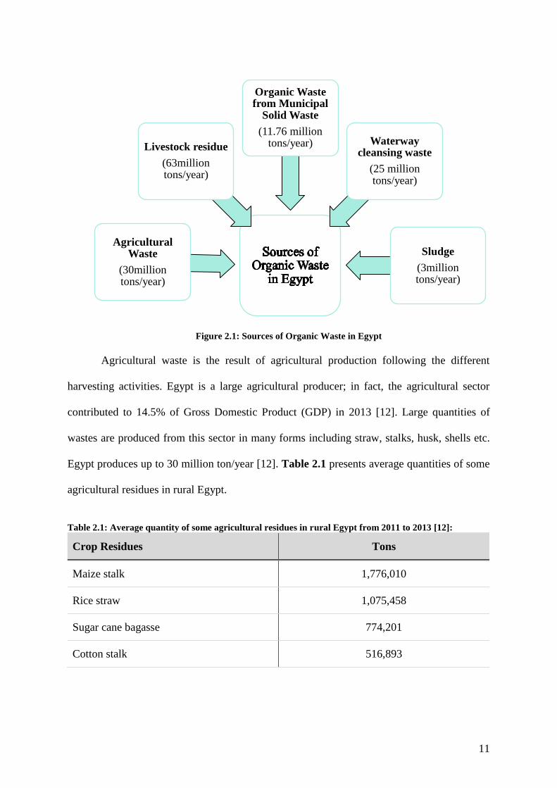
cleansing waste (dredging, floating weeds, etc.) as shown in Figure 2.1 and fully described
below.
11
Figure 2.1: Sources of Organic Waste in Egypt
Agricultural waste is the result of agricultural production following the different
harvesting activities. Egypt is a large agricultural producer; in fact, the agricultural sector
contributed to 14.5% of Gross Domestic Product (GDP) in 2013 [12]. Large quantities of
wastes are produced from this sector in many forms including straw, stalks, husk, shells etc.
Egypt produces up to 30 million ton/year [12]. Table 2.1 presents average quantities of some
agricultural residues in rural Egypt.
Table 2.1: Average quantity of some agricultural residues in rural Egypt from 2011 to 2013 [12]:
Crop Residues Tons
Maize stalk 1,776,010
Rice straw 1,075,458
Sugar cane bagasse 774,201
Cotton stalk 516,893
Agricultural Waste
(30million tons/year)
Livestock residue
(63million tons/year)
Organic Waste from Municipal
Solid Waste
(11.76 million tons/year) Waterway
cleansing waste
(25 million tons/year)
Sludge
(3million tons/year)
12
It is worth mentioning that Delta region generates the highest amount of residues is,
followed by Upper and Middle Egypt regions. According to Kamel et al. [12], the governorates
of El-Behera, Sharkeia, Dakahlia and Kafr el Sheikh in the delta region generates between 0.59
to 0.87 million tons of agriculture residues every year. Middle Delta region generates a high
amount of maize stalk, rice straw and cotton stalk, while Upper Egypt region like Qena and
Asswan generate large amounts of sugar cane bagasse [12].
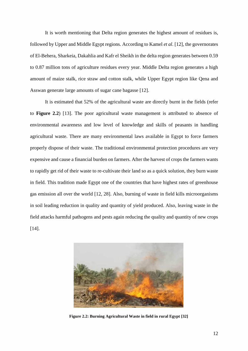
It is estimated that 52% of the agricultural waste are directly burnt in the fields (refer
to Figure 2.2) [13]. The poor agricultural waste management is attributed to absence of
environmental awareness and low level of knowledge and skills of peasants in handling
agricultural waste. There are many environmental laws available in Egypt to force farmers
properly dispose of their waste. The traditional environmental protection procedures are very
expensive and cause a financial burden on farmers. After the harvest of crops the farmers wants
to rapidly get rid of their waste to re-cultivate their land so as a quick solution, they burn waste
in field. This tradition made Egypt one of the countries that have highest rates of greenhouse
gas emission all over the world [12, 28]. Also, burning of waste in field kills microorganisms
in soil leading reduction in quality and quantity of yield produced. Also, leaving waste in the
field attacks harmful pathogens and pests again reducing the quality and quantity of new crops
[14].
Figure 2.2: Burning Agricultural Waste in field in rural Egypt [32]
13
In addition to the agricultural waste, there is also livestock residues, which consists of
chicken and cattle manure. According to the FAO (Food and Agriculture organization of the
United Nations) 2017 report [33], it is estimated that around 57million tons of cattle manure
and 6 million tons of chicken manure are produced each year. The highest cattle manure
production is found in the Middle Delta region, at 31 million tons per year (55% of total manure
production in Egypt). Upper Egypt region generates 13 million tons of cattle manure per year
(23%) followed by the Middle Egypt region, which produces 10 million tons (19 %) [33].
Another source of organic waste is municipal solid waste (MSW). According to the
country report on the solid waste management in Egypt in 2014 [11], Egypt generates 21million
tons of MSW per year from which 56% are organic waste (equal to 11.76 million tons per
year). Also, 25million tons per year of waterway cleansing waste and 3million tons of sludge
are generated in Egypt [11].
2.1.2. Huge amounts of Municipal Solid Waste
Another serious problem rural villages suffer from is poor MSW management. A large
portion of the MSW are dumped in open dump sites, waterways and/or streets causing
extensive health, ecological and environmental problems. As previously stated, Egypt
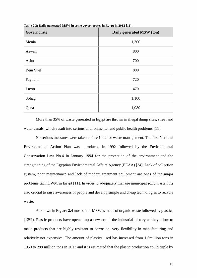
generates 21million tons of MSW per year and its composition is illustrated in Figure 2.4.
Table 2.2 also shows the daily amount of MSW generated in some of the Upper and Middle
Egypt regions.
14
Figure 2.3: Municipal Solid Waste dumped in waterways, in Egypt
Figure 2.4: MSW Composition in Egypt [11]
15
Table 2.2: Daily generated MSW in some governorates in Egypt in 2012 [11]:
Governorate Daily generated MSW (ton)
Menia 1,300
Aswan 800
Asiut 700
Beni Suef 800
Fayoum 720
Luxor 470
Sohag 1,100
Qena 1,080
More than 35% of waste generated in Egypt are thrown in illegal dump sites, street and
water canals, which result into serious environmental and public health problems [11].
No serious measures were taken before 1992 for waste management. The first National
Environmental Action Plan was introduced in 1992 followed by the Environmental
Conservation Law No.4 in January 1994 for the protection of the environment and the
strengthening of the Egyptian Environmental Affairs Agency (EEAA) [34]. Lack of collection
system, poor maintenance and lack of modern treatment equipment are ones of the major
problems facing WM in Egypt [11]. In order to adequately manage municipal solid waste, it is
also crucial to raise awareness of people and develop simple and cheap technologies to recycle
waste.
As shown in Figure 2.4 most of the MSW is made of organic waste followed by plastics
(13%). Plastic products have opened up a new era in the industrial history as they allow to
make products that are highly resistant to corrosion, very flexibility in manufacturing and
relatively not expensive. The amount of plastics used has increased from 1.5million tons in
1950 to 299 million tons in 2013 and it is estimated that the plastic production could triple by
16
2030 [35]. Yet, the production of plastic waste has been an important issue due to the pollution
and environmental impact of poor disposal of plastics. Dumping of plastic waste in open areas
is still the most commonly used disposal method in developing countries. Plastics are divided
into thermoplastics and thermosets, there is no data about the amount of each one separately
generated in Egypt. Thermoplastics can be easily recycled as they melt once subjected to heat;
however, thermosets are harder to recycle as they do not melt when heated. That’s why
thermosets are referred to as rejects.
Another type of reject is packaging materials. Packaging material could be made of
paper and cardboard, glass, aluminum, plastics or laminated packaging material. The laminated
packaging material are usually the ones referred to as rejects as they are hard to recycle because
they are made of multilayer films of different materials bonded together. The Central
Department of Solid Waste estimate that around 29% of MSW in Egypt could be made of
packaging materials, which represents 6 million tons [11]. This percentage is not clearly stated
in Figure 2.4 as laminated packaging materials are made of different types of materials
including aluminum, plastic and binding material. Therefore, some of these waste could be
found under plastics, metals and others in Figure 2.4. Research effort is still needed to find
ways to easily recycle rejects.
2.1.3. Other important problems
In addition to poor management of organic waste and MSW, rural areas in Egypt suffer
from other issues including lack of infrastructure. Large part of Egypt is connected to supply
water network; however, many rural villages do not have access to drainage system. The
Egyptian government has invested a lot in supplying water to households all over the country
increasing dramatically water usage. Yet, only 4% of the Egyptian villages have proper
drainage systems [36, 37, 38]. This large discrepancy between water supply and sanitary
drainage force residents of rural village dispose of their wastewater in an informal way. Most
17
of wastewater are dumped in streets, waterways, or irrigation drainage network. People usually
use septic tanks to collect their wastewater, which are usually not properly sealed. Thus,
wastewater leaks and pollutes surrounding ground water. Unfortunately, this contaminated
water is usually used for irrigation and/or drinking. Abdel Wahed et al. [39] studied the water
quality in Fayoum and concluded that both drinking and irrigation water are contaminated and
have high values of BOD, COD, metals and TSS. This is because people directly throw their
wastes in waterways.
This practice caused not only poor water quality but also caused many dieses including
typhoid, diarrhea, bilharizia, hepatitis C. In fact, water contamination along with poor hygiene
causes around 88% percent of reported cases of diarrhea worldwide [40]. WHO stated that
25.1% of diseases can be reduced by improving the quality of water and having better hygiene
[41].
In addition to all of the above-mentioned problems, rural villages in Egypt suffer from
poverty, low standard of living, health problems, illiteracy and unemployment [29]. Also,
housing conditions are far from satisfactory. Houses in rural Egypt usually consists of mud or
red bricks houses, which are very close to each other and roofing is usually made of reeds,
which led rain through and often catch fire [42].
2.2. Traditional Methods of Waste Disposal
The rapid increase in population and economic growth has led to an increase in the
generation of waste. Consequently, several methods have been developed to safely dispose of
waste including waste reduction and waste recovery for reuse, recycling, incineration and
landfilling. The most common ways of waste disposal internationally are incineration and/or
landfilling. Incineration is a process in which solid waste is burnt and converted to ash. This
process allows to reduce the waste volume. The produced ash is usually landfilled. The
landfilling process uses polyethylene, high-density polyethylene and polyvinyl chloride as
18
liner, it also required a leachate collection system, biogas collection system as well as a storm
water drainage system. Several environmental protection laws and regulations are drafted and
adopted in Egypt to force the proper and safe waste disposal. However, these disposal
techniques and environmental protection procedures are seen as a burden and not properly
implemented. According to the country report on the solid waste management in Egypt in 2014,
only 30% of MSW is collected in rural areas and 50-65% in urban areas. Only 7% of the MSW
is composted and 10-15% recycled, 7% landfilled and the rest end up in open dump sites [11].
In Egypt there are 22 planned sanitary landfills from which 2 are under construction and 7
operational [11]. The main disadvantage of incineration and landfilling processes is that they
require high capital, high running costs, and most importantly they deplete natural resources
causing them to be unsustainable [43]. In developing countries like Egypt, landfills have not
been very successful because they are poorly controlled causing negative effects on the
environment from the formed leachate [44]. Some of these impacts include fires, explosions,
soil degradation, unpleasant odor, groundwater pollution, air pollution due to GHG emissions
as well as scarcity of land [45, 44, 46]. Instead of properly disposing of waste, most of the
wastes generated are either burnt or end up in open, public and random dumpsite or water
canals, which contribute to the health, ecological and environmental problems especially in
rural areas. Unfortunately, very few literatures are giving attention to optimize and study
possible innovative solutions for sustainable waste management in rural villages in developing
countries like Egypt [46]. Therefore, it is an essential aspect to consider approaching 100 %
full utilization of wastes and develop sustainable solutions in rural villages in Egypt in order
to help in the development of these areas.
2.3. Sustainability
The concept of sustainability was developed in 1972 during the United Nations
Conference on Human Environment. The first definition of the term ‘sustainable development’
19
appeared in publication of Brundtland Report entitled ‘Our Common Future’ as the
“development that meets the needs of the people today without compromising the ability of
future generations to meet their own needs” [47]. After that, considerable efforts were made to
implement the concept of sustainability in many fields. Indeed, Sustainable Seattle, a non-profit
organization promoting sustainability, has defined Sustainable Development as “economic and
social changes that promote human prosperity and quality of life without causing ecological or
social changes” [5]. From the definition of sustainable development, it is clear that all plans
should allow a collaboration between environmentalist, research institutes, policy makers,
businessmen and society.
Based on the tragic situation – refer to Chapter 1 – in rural Egypt and the definitions of
sustainability, rural communities in Egypt can be called “unsustainable”. Rural communities
in Egypt can be described as an open system as they consume natural resources and produce
waste and this generated waste is poorly managed. To reach sustainability, it is imperative to
introduce the concepts of cradle-to-cradle, industrial ecology, environmentally balanced
Industrial Complex to reach sustainable development in rural communities in Egypt.
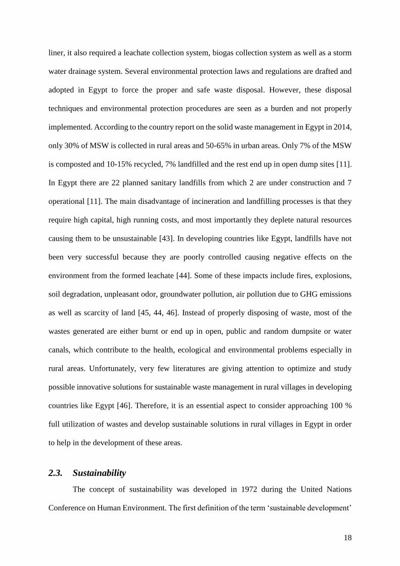
2.3.1. From Cradle-to-Grave to Cradle-to-Cradle
The industrial sector has been following a linear model known as “Cradle-to- Grave”
illustrated in Figure 2.5. In this model, new products are made from raw material resources
and at the end of their life they are thrown away.
20
Figure 2.5 - Cradle- to- Grave Approach [43]
In order to make profits, many companies followed the concept of “built-in-
obsolescence”, in which products are designed for a limited period of time. After certain period
of time buying a new product becomes cheaper than repair old product using old technology.
Also, large amount of material is wasted in packaging that do not have any function except
attracting the attention of the buyer and the material waste almost immediately. By following
this strategy to sell more products, sellers are overlooking ecological and long-term impact of
the huge amount of waste generated and depletion of natural resources.
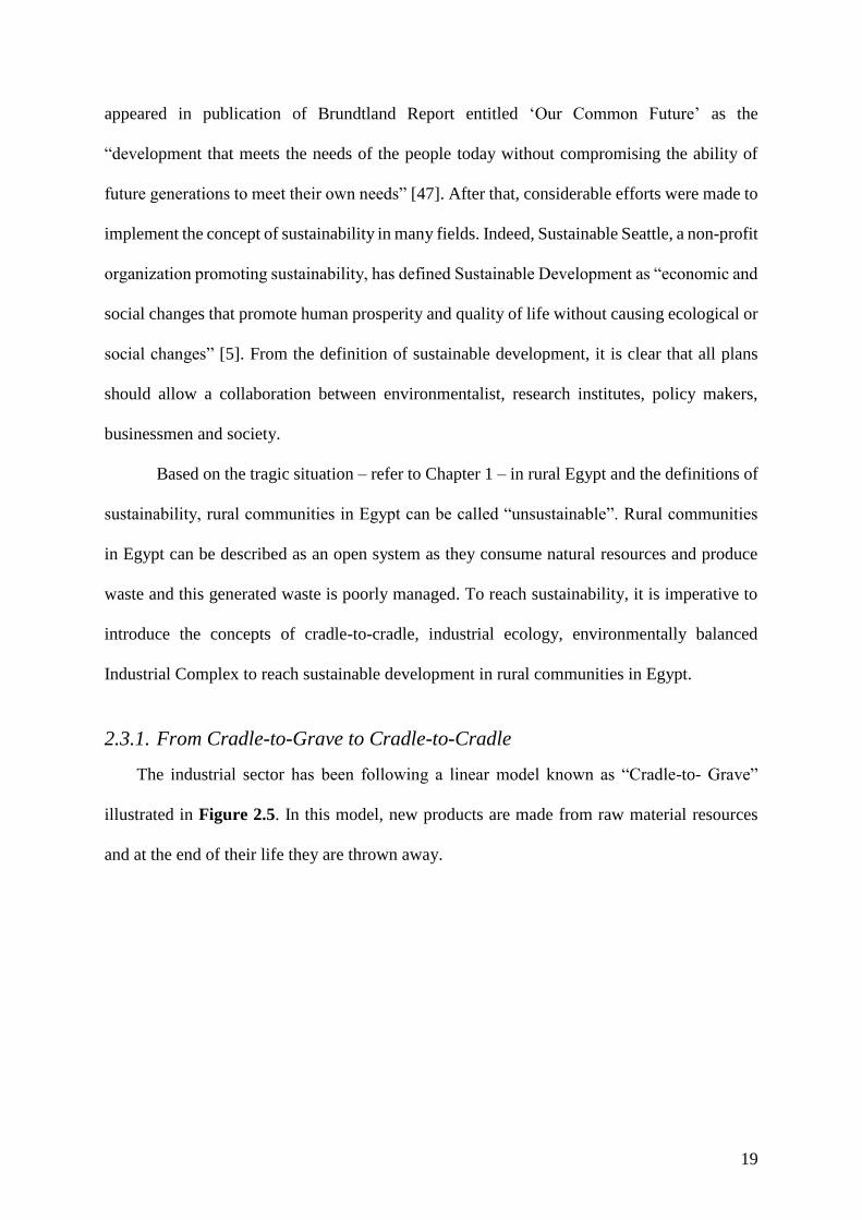
The concept of cradle-to-cradle is proposed by McDonough and Braungart [48], it consists of
infinitely using waste for the production of new goods. McDonough and Braungart made the
papers of their book entitled “Cradle-To-Cradle: Remaking the way we make things” out of
recycled plastic set a practical example for the concept of cradle-to-cradle. This concept of
C2C is illustrated in Figure 2.6. Following this concept, will allows to reduce waste generated
every year as well as ensure a sustainable source of high-quality material.
Extraction of raw
material Manufacturing
Transport
Packaging and
marketing
Reduce, reuse, and
recycle Final
disposal
Cradle
Grave
Cradle-to-
Grave
21
Figure 2.6 – Cradle-to-Cradle Approach [43]
2.3.2. Industrial Ecology (IE) and Eco-Industrial Park (EIP)
The concept of Industrial Ecology (IE) was defined by Frosch and Gallopoulos in 1989
to reach sustainable development. It is defined as a system in which “energy and materials is
optimized, waste generation is minimized, and the effluents of one process […] serve as the
raw material for another” [49]. This concept was inspired by the natural ecosystem cycle [37].
As industrial waste is non-biodegradable, it is imperative to produce goods were waste of one
industry can be the raw material of another [51], and have a cyclical flow of material [52].
Industrial ecology will make the not only solve the waste problem, but also will reduce the cost
of raw material used in industry. Applying this concept will open the road to “niche industries”,
serving the main industry, to grow [51]. These new industries will buy and sell waste, which
will reduce the amount of waste generated and maximize their reuse. Industrial Ecology;
therefore, promotes sustainable industries in a sustainable society.
Preparation of
raw material
Processing of raw
material
Transport
Packaging and
marketing
Use of Product
On-site
recycling
Off-site
recycling
Other
industries
22
The concept of Industrial Ecology has been applied in the industrial sector by
developing Eco-Industrial Parks (EIP). In this park any waste generated from an industry is
reused or recycled to ensure sustainable development. EIPs are a direct application of the
industrial ecology approach. The main aim of EIP is to group different industries in one
location in order to minimize energy and material waste. Many research indicate that
sustainable development of the economy can be promoted via implementation of a
successful eco-industrial park [53].
2.3.3. Environmentally Balanced Industrial Complex (EBIC)
The concept of Environmentally Balanced Industrial Complex (EBIC) was developed
by Nemerow and Dasgupta in 1986. Nemerow defined EBIC to be “a selective collection of
compatible industrial plants located together in one area (complex) to minimize both
environmental impact and industrial production costs” [54]. Unlike EIPs, the EBIC proposes
to group compatible industries large and or small industries in one area close to each other. By
doing that different industries will use the waste of each other to produce new goods. This
complex will not only minimize waste generated by industries but also will reduce the cost of
raw material, transportation, storage, and waste disposal and treatment.
2.3.4. Green Economy (GE)
Green economy is a new model for the economic development based on sustainable
development and knowledge of ecological economics. The UN Environment Program (UNEP)
defines the green economy as “one that results in improved human well-being and social
equity, while significantly reducing environmental risks and ecological scarcities” [55]. The
aim of green economy is to reach a win-win solution and provide economic, social and
environmental well-being.
23
2.3.5. Sustainable Development Goals
Reference to “Sustainable Development Strategy: Egypt Vision 2030” report prepared
by the Minister of Planning, Monitoring and Administrative Reform in 2015, one of the main
goals of Egypt is “to preserve natural resources and support their efficient use and investment,
while ensuring next generations’ rights. A clean, safe and healthy environment leading to
diversified production resources and economic activities, supporting competitiveness,
providing new jobs, eliminating poverty and achieving social justice” [9].
Also, the United Nations has developed seventeen sustainable development goals for 2030
including the following [10]:
Goal 3 – Good health and well being
Goal 6 – Clean water and sanitation
Goal 8 – Decent work and economic growth
Goal 11 – Sustainable cities and communities
Goal 12 – Responsible consumption and production
As mentioned in chapter 1, around 56.9% of the Egyptian population lives in rural areas;
therefore, to contribute to these goals it is imperative to help rural villages reach sustainable
development and not only focus on urban development.
2.4. Composting of organic waste
Biodegradable material or organic waste usually accounts for over 50% of the MSW
stream in developing countries. In fact, as previously mentioned, in Egypt 56% of the MSW is
organic. Other types of organic waste include agricultural waste, livestock residue, waterway
cleansing, sludge, etc., which represent around 133million tons of waste/year (Figure 2.1).
Hence, there has been an increasing attention on improving the management of organic waste.
The composting process is considered one of the most suitable alternatives to manage and treat
organic solid waste [18, 19, 20]. This process occurs in nature, called rotting, but slowly. The
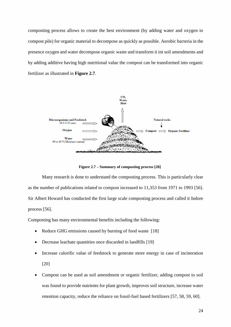
24
composting process allows to create the best environment (by adding water and oxygen to
compost pile) for organic material to decompose as quickly as possible. Aerobic bacteria in the
presence oxygen and water decompose organic waste and transform it int soil amendments and
by adding additive having high nutritional value the compost can be transformed into organic
fertilizer as illustrated in Figure 2.7.
Figure 2.7 – Summary of composting process [28]
Many research is done to understand the composting process. This is particularly clear
as the number of publications related to compost increased to 11,353 from 1971 to 1993 [56].
Sir Albert Howard has conducted the first large scale composting process and called it Indore
process [56].
Composting has many environmental benefits including the following:
Reduce GHG emissions caused by burning of food waste [18]
Decrease leachate quantities once discarded in landfills [19]
Increase calorific value of feedstock to generate more energy in case of incineration
[20]
Compost can be used as soil amendment or organic fertilizer, adding compost to soil
was found to provide nutrients for plant growth, improves soil structure, increase water
retention capacity, reduce the reliance on fossil-fuel based fertilizers [57, 58, 59, 60].
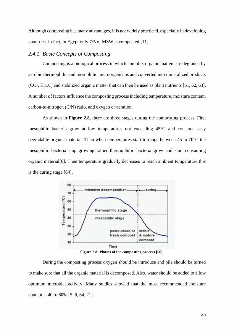
25
Although composting has many advantages, it is not widely practiced, especially in developing
countries. In fact, in Egypt only 7% of MSW is composted [11].
2.4.1. Basic Concepts of Composting
Composting is a biological process in which complex organic matters are degraded by
aerobic thermophilic and mesophilic microorganisms and converted into mineralized products
(CO2, H2O, ) and stabilized organic matter that can then be used as plant nutrients [61, 62, 63].
A number of factors influence the composting process including temperature, moisture content,
carbon-to-nitrogen (C/N) ratio, and oxygen or aeration.
As shown in Figure 2.8, there are three stages during the composting process. First
mesophilic bacteria grow at low temperatures not exceeding 45°C and consume easy
degradable organic material. Then when temperatures start to range between 45 to 70°C the
mesophilic bacteria stop growing rather thermophilic bacteria grow and start consuming
organic material[6]. Then temperature gradually decreases to reach ambient temperature this
is the curing stage [64].
Figure 2.8: Phases of the composting process [56]
During the composting process oxygen should be introduce and pile should be turned
to make sure that all the organic material is decomposed. Also, water should be added to allow
optimum microbial activity. Many studies showed that the most recommended moisture
content is 40 to 60% [5, 6, 64, 21].
26
The presence of carbon (C) and nitrogen (N) is very important to ensure optimum
microbial activity. Studies showed that the recommended C/N ratio is between 20:1 to 30:1 [6,
64]. In other words, for each nitrogen part microbes consume between 20 to 30 parts of carbons.
A low C/N ratio does not allow efficient micro-organism activity and incomplete nitrification
process, which cause pile to have bad odor [6, 5]. In fact, Hansen et al. [67] reported that
ammonia emission from the poultry manure was four times greater than piles with C/N ratio
of 20. If the C/N ratio is too high, the decomposition process will slow down [64].
Composting involve aerobic bacteria so continuous supply of oxygen is crucial for the process
to occur. Many research has been conducted to find the best aeration rate. But results of these
studies are quite different, some studies suggested rates as low as 0.04-0.08L air/min-kg [68],
while other studies recommended ranges as high as 0.87-1.87 air/min-kg [69]. There are
different techniques used to aerate the compost pile including [5]:
Natural composting in which compost piles are manually turned.
Passive composting consists of having perforated PVC pipes at the bottom of the
compost piles to introduce air to pile without having to turn it.
Forced composting is similar to the passive composting process, in this process PVC
pipes are connected to a blower to ensure that continuous air supply at constant velocity
are introduced at the center of the pile.
Yet, composting has some disadvantages including the following:
Composting is a time-consuming process that can take up to six months [21, 6, 70]
Composting can create unstable product quality [21] and composts should be in high
degree of maturity and stability to be safely applied on agricultural lands without any
adverse effect [71]
Composting is a complex process and there are still knowledge gaps in understanding
the process due to the high variety and heterogeneity of feedstock
27
In rural areas large portions of land are used to dump wastes also these villages suffer from
extensive pollution. Therefore, it became of high importance to develop a method to accelerate
the composting process, while having a stable and high-quality product at the end [71].
Therefore, many research efforts have been made in field of composting [72, 73, 74, 75, 76,
77, 78].
2.4.2. Composting of Rice Straw
Rice is the third most important grain crop in the world behind wheat and corn. Based
on FAO statistics, the global production of rice was estimated to be 650 million tons in 2007
[79]. Every kilogram of harvested rice generates around 1-1.5 kg of straw, which makes rice
straw one of the most abundant lignocellulosic waste materials in the world [80]. Egypt is an
agricultural country and the largest producer of rice in Africa. It is estimated that around
5.9million tons of rice straw were generated in 2013 [17]. A portion of the rice straw is mainly
used as fuel for cooking and house heating, animal feed, fiber for pulping and plowing into
farmland. A large amount of rice straw is dumped and burned. In Egypt, it is estimated that
about 3.1million tons per year of rice straw are disposed of by directly burning in open fields
causing serious environmental problems, including air pollution and soil degradation due to
lack of cost-effective treatment approaches [16, 17]. Rice straw contains cellulose and
hemicellulose and lining. Several studies showed that rice straw could be used to produce high
value-added products via composting process [81, 82]. Yet, stable and mature organic fertilizer
is hard to obtain with rice straw as it is difficult to degrade and a variety of micro-organisms
type is involved in the composting process [83, 84, 85, 86]. Therefore, there had been many
research effort to improve the quality of composting of rice straw and increase rate of
composting process [87, 76, 17, 78].

28
2.4.3. Methods to improve composting process
Many studies have been done to develop methods to accelerate and improve
composting process. One method is to develop closed-type bioreactors in which all factors
affecting composting process are optimized (temperature, humidity, aeration, pH values, C/N
ratio, etc.) [21]. However, this method is expensive.
Another-way is co-composting of agriculture waste or food waste with animal manure.
Some studies have reported the effect of animal manure on composting process [88]. Dehshan
et al. [89] reported that co-compost of cattle manure with rice straw at ratio of 4:1 produced an
organic matter, total nitrogen and C/N ratio contents suitable for soil amendment. Abdelhamid
et al. [90] reported that 20 to 30% of poultry manure on rice straw can form high quality soil
amendment. Zhang and He [91] investigated the properties of co-composting pine staw and
swine manure and reported that addition of 30% of swine manure while maintaining the C/N
ratio at 40 produces high quality composts. Li et al. [64] added animal manure to rice straw
and investigated the effect of different composting parameters including oxygen introduction
method and rate, moisture content and manure age on the properties of final product.
Ogunwande et al. [92] studied co-composting of raw chicken manure and saw-dust and found
that incrasing C/N ratio and aeration rate increases the moisture loss of the pile. Also,
significant organic waste degradation and caused loss of total nitrogen via ammonia
volatilization and decrease in total carbon losses. Tiquia et al. [93] reported that co-composting
of poultry manure and yard trimmings showed increase in micro-organisms activity level, and
removal of phytotoxicity. Quian et al. [71] reported that co-composting of swine and rice straw
(60% swine manure 40% rice straw) and dairy manure and rice straw (67% dairy manure and
33% of rice straw) results into higher maturation rates.
In addition to co-composting, some studies showed that inoculation of compost piles
with microbial additives can accelerate the composting process and increase nutritional value
29
of final compost. Some countries, like China and Egypt, have produced commercial microbial
inoculants mainly containing lactic acid bacteria, yeasts and photosynthetic bacteria and are
available in the local market. Yet, the scientific data for the type of strains and their
composition are often not revealed and generally remained as trade secrets. No published
studies have reported their exact composition nor their effects on composting process.
Another widely known microbial additive is Effective micro-organisms (known as
EM.1). Professor Dr. Teruo Higa developed EM in 1970s at Ryukyus University, Okinawa,
Japan [94]. It consists of various strains of naturally occurring anaerobic nontoxic and non-
pathogenic microorganisms in a carbohydrate-rich liquid carrier substrate (molasses nutrient
solution). It is mainly composed of three main groups of micro-organisms: (1) photosynthetic
bacteria - synthesis useful substances like amino-acid, nucleic acid, bioactive substance and
sugars from organic matter and harmful gases (H2S), which promote plant growth and
development, (2) lactic acid bacteria - these bacteria produce lactic acid from sugars and
carbohydrates, which suppresses harmful microorganism and enhance decomposition of
resistant materials (cellulose) and removes undesirable effects of decomposition, (3) Yeast -
synthesize anti-microbial and other substances required for plant growth from amino-acids and
sugars produced by photosynthetic bacteria [95]. However, its exact composition is very
complex and remains a secret.
Jusoh et al. [94] evaluated the effect of adding 5% of commercial EM on the
composting pile having rice straw and goat manure and green waste. The study indicated that
compost with EM has higher nutritional value compared to compost without EM.
Lim et al. [96] reported the effect of inoculating oil palm fruit bunches with commercial
EM. The study indicated that adding EM improves decomposition. In fact, lower total organic
carbon content and C/N ratios were recorded at the end of the composting process in compost
pile with EM compared to compost pile without EM.
30
On the contrary, Fan et al. [97] reported that EM do not have significant effect on composting
of food waste at home scale.
Few studies have also reported the effect of specific types of bacteria on the composting
process. Abdel-Rahman et al. [17] evaluated the effect of applying two types of bacteria
(Bacillus licheniformis and Bacillus sonorensis) maturation time and quality of compost
produced by composting rice straw and cattle manure. This study indicated that these additives
improved the composting maturation time and increase the nutrient content of final compost.
Also, Abdel-Rahman [15] developed a solution mainly containing two types of bacteria,
Bacillus amyloliquefaciens and Bacillus licheniformis. This solution showed improvement in
rice straw composting and gave results that are comparable to the ones obtained using EM.
Also, this study showed that addition of natural rocks including dolomite, feldspar, rock
phosphate and zinc enhance the decomposition process.
Gou et al. [98] investigated the effect of a consortium of psychrotrophic bacteria and
thermophilic fungus as inoculant for dairy manure-rice straw composting in cold climate. The
study revealed that this microbial additive accelerated the start of composting under cold
climate conditions. Also, more prolonged thermophilic phase was observed, and compost
reached maturity with greater decrease in total organic carbon and C/N ratio, as well as a higher
increase in total nitrogen and germination index.
In addition to microbial additives, several recent studies showed that biochar could have
positive effects on the composting process. Biochar is produced via pyrolysis of biomass
residues under limited oxygen conditions [99]. Currently biochar is used in many applications
including soil improvement, carbon sequestration, energy production, and pollution
remediation [100, 101]. Very few studies have evaluated the effect of biochar on organic waste
composting. Several advantages have been reported including: (1) improving aeration
conditions as biochar is porous material and allow oxygen to enter the pile[102] , (2) reducing
31
odors and greenhouse gases emissions [103, 102], (3) reducing ammonia nitrogen losses [104],
(4) accelerating the decomposition and humification of organic matter [103, 102, 105], (5)
improving the quality of end compost [106], (6) reducing heavy metals in soil [107], (7)
enhancing micro-organisms activity level [108]. Some studies have shown that biochar has
great potential for remediate the soil contaminated with organic pollutants and heavy metals
[109, 110, 111, 112, 113]. However, multi-contaminated soil may require addition of other soil
amendments to help reduce heavy metal availability and improve soil fertility [114]. Some
studies have shown that the application of biochar is inexpensive and sustainable and can have
positive impact on soil remediation and plant growth [115]. Several studies reported
application of biochar with doses from 2% to 50% [116]. According to Sanchez Monedero et
al., the recommended application dose of biochar to compost is around 10% [78]. Some studies
have also reported use of higher doses up to 50%; however, some authors have reported that
doses higher than 20% can slow down the composting process [117].
As presented above, composting is one of the ideal ways to recycle the huge amount of organic
waste generated in rural villages in Egypt. However, composting is time consuming process
Unfortunately, very few research studies reported the effect of these different additives on
composting of organic waste like rice straw. Therefore, it is essential to study the effect of
these different additives on composting of organic waste like rice straw.
2.5. Recycling of thermosets and packaging materials
As previously discussed, another serious problem rural villages suffer from is poor
MSW management, which contribute to many problems facing rural communities. Most of the
MSW is composed of organic waste followed by 13% of plastic waste,10% of paper/cardboard,
4%glass, 2%metal, and 15%other types of material including composite materials (refer to
Figure 1.4). This research focus on recycling of two types of materials that are difficult to
recycle and referred to as rejects or unrecyclable: thermosets and packaging materials.

32
2.5.1. Recycling of thermosets
Plastics also known as polymers are material that can be shaped or molded by heat.
Although the use of plastic has many technological advantages, the extensive use of plastics
causes serious environmental problems as they are non-biodegradable. Their impact on
environment is very harmful if it is burnt it causes air pollution. There are two types of
polymers: (1) thermoplastics that consist of individual long-chain molecules that are easily
recycled as they melt once subject to heat, and (2) thermosets that contain highly cross-linked
three-dimensional network, which makes it tedious to recycle as they do not melt once heated.
Nowadays, thermosets are used in a wide range of applications including adhesives,
coatings, polymer composites, electrical insulation, printed circuit boards, etc. Yet, the
recycling at the end of their life cycle is a very difficult challenge because of their cross-linked
nature. Once heated thermosets decompose and degrade unlike thermoplastics. As thermosets
are perceived as difficult or impossible to recycle, there have been suggestions to avoid their
use. Yet, their attractive properties (high hardness, thermal resistance, insulation, etc.) make
them significantly used in many applications. Therefore, most of the thermoset products end
up in landfills or are incinerated at the end of their life, which causes serious environmental
concerns due to the fact that plastic waste contains various toxic elements, which can pollute
soil and water [23, 24].
Due to the increasing environmental concern, recycling of non-biodegradable
thermoset wastes has been the major issue for researchers for the last two decades [25]. In
2011, Thomas et al. [118] proposed a comprehensive review about methods of recycling of
thermosets and their composites. There are two types of thermosets: (1) hard thermosets and
(2) elastic or rubber thermosets.
33
Hard thermosets
Hard thermosets have Van der Waals bonds (weak bonds) and have a stronger covalent
bonds linking chains together. This "cross-linking" between the chains prevent the material to
soften once heated. In the case of thermoplastic polymers chains are linked together via weak
bonds, which make these materials softened when subject to heat. So they can be heated and
remolded and once they cool down they take the shape of the mold and recover their initial
properties.
Thermosets are generally stronger than thermoplastics due to the three-dimensional
network bond. They are used in high-temperature applications. However, they are more brittle
than thermoplastics. Since their shape is permanent, they are very hard to recycle as a source
of newly made plastics.
There are several types of hard thermosets such epoxy, Phenol- formaldehyde and
melamine formaldehyde etc. Many published papers have reported different techniques to
recycle epoxy and epoxy composites. However, few papers have investigated recycling of
melamine formaldehyde. Melamine formaldehyde is made from the polymerization of
formaldehyde (chemical formula CH2O) with melamine (chemical formula C3H6N6). Excess
melamine forms three-dimensional network structure with further quantities of melamine
monomer.
Melamine formaldehyde is characterized by superior properties. The melamine is water
repellant, has good electrical properties and has high heat resistance. It has a wide color range,
track resistance and scratch resistance. It is used in many applications including tableware,
electrical applications and knobs and handles for kitchen utensils.
Recycling of hard thermosets
Several recycling methods of thermosets have been investigated including mechanical,
thermal, and chemical approaches [101].
34
Mechanical recycling is a basic technology which can be incorporated into new sheet
moulding compounds (SMC) parts [103], in a thermoplastic matrix [104], or in concrete [102,
100]. Petterson and Nilsson [119] studied the addition of recycled car bumpers into the SMC
to produce new car bumpers. The bumpers have been grounded to form particle size ranging
from 200m to 1mm. Ground material have been added to SMC (10% ground material – 90%
raw material), it was found that this method increased flexural strength of bumpers.
Kouparitsas et al. [120] produced new composite material having high tensile strength by
adding grounded polyester and epoxy composites to thermoplastic matrix. Chaitongrat and
Siwadamrongpong [23] found that adding 25% of melamine formaldehyde waste powder (as
fine aggregate to partially replace river sand) could produce high compressive strength light
weight concrete. The study showed that adding 25% of melamine formaldehyde waste powder
could produce high compressive strength concrete that comply with ASTM standard for non-
load-bearing lightweight concrete.
Chemical processes have been investigated as well; however, these methods involve
the use of strong chemicals at high pressure and relatively high temperature [121, 122], which
limits its spread and large-scale uses. Recently, Kuang et al. [123] developed a chemical
solvent that can quickly dissolve epoxy. Also, La Rosa et al. [124] developed a chemical
technique using acetic acid recycling bath of 70 °C for 1 h to transform epoxy thermoset into
thermoplastic.
Other methods that have been reported to recycle thermosets are composites thermosets
are recycled using: (1) incineration, (2) co-incineration in cement kilns, (3) pyrolysis consisting
of heating material in an oxygen free atmosphere in order to recover polymer as oil [125].
Mechanical recycling has many advantages compared to the previously presented
recycling methods. In fact, mechanical size reduction is a simple, inexpensive technique that
does not have any environmental impacts [125].
35
Synthetic Rubbers
Rubber provided tremendous benefits because of its unique properties related to its
cross-linked structure as well as very high elasticity, which resulted from vulcanization process
[126]. Due to these outstanding properties, rubber is used in many fields an applications
including automotive and electronics manufacturing [127, 128]. There are many types of
rubber available in the market including natural rubber (NR), styrene-butadiene rubber (SBR),
nitrile, ethylene-propylene-diene monomer (EPDM) rubber, etc. Therefore, rubber waste is
found in many forms such as scrap tires, inner tubes, discarded and rejected rubber glove,
balloons, rubber bands, shoe soles, mattresses, hoses, seals, gaskets, diaphragms etc. However,
the complex structure and high properties of rubber makes it very difficult to recycle or degrade
it.
According to the International Rubber Study Group, the world total rubber consumption
in 2017 is 28.05million tons and this number is expected to increase by a rate of 2.8% annually
from 2017 to 2025 [129]. Due to these significant increase of rubber products, rubber waste is
becoming a serious problem. Most of rubber waste is landfilled or dumped in open dump sites
as an easy and cheap solution leading to many environmental problems [130]. Therefore, many
research efforts have been made in waste management of waste rubber.
Recycling of waste rubber
Large volume of waste tyres are generated every year [130]. Sustainable utilization of
waste tyres has been studied extensively in recent years. Nuzaimah et al. [130] and Ramarad
et al. [131] published a comprehensive review regarding the utilization of waste rubber as
filling material that indicated that waste tyres can be used in many applications.
Abu Jyadil et al. [132] developed a composite material made of polyester as the matrix
and rubber tyres particles as the filler. Rubber concentration up to 40% was added to polyester
and material thermal conductivity, water retention, density, thermal stability and micro-
36
structure have been investigated. The study revealed that this composite material has the
potential to be used as thermal insulator in constructive applications as the composite material
produced has high mechanical properties comparable with the currently used material as well
as has relatively low thermal conductivity and low water absorption.
Shu and Huang [133] published a comprehensive review of the use of waste tyres into
asphalt paving. The literature review conducted indicated that the use of rubber tyres waste in
asphalt have been extensively studied and have been reported to be successful due to the
compatibility and interaction between rubber particles and asphalt binder.
Yang [135] reported the use of waste tyres as fillers in drainage structures such as for
underground and horizontal drain.
Svoboda et al. [136] highlighted the use of that waste tyres as filler in concrete. The
study revealed that waste tyres can improve the properties of concrete such as ductility,
damping, acoustic and impact resistance.
In addition to waste rubber tyres, some research studies revealed the possibility of using
other types of rubber waste in different applications. Guendouz and Boukhelkhal [137]
investigated the use of rubber obtained from old shoes sole to partially replace sand concrete.
The results indicated that rubber waste particles increased the workability and reduce the bulk
density of sand concrete and improved the thermal insulation performances of sand concrete.
Also, Riyajan et al. [128] showed that use of rubber gloves as filling material increase impact
strength, tensile strength and decrease stiffness of materials.
As presented above, many studies reported the use of waste tyre to produce new goods.
s. Yet, recycling of other types of rubbers is very limited. After tyres, ethylene-propylene-
diene- monomer (EPDM) represents the second largest type of elastomeric material thrown
away. However, very few studies reported the use of EPDM rubber in the production of new
goods. EPDM has many good properties such as excellent resistance to heat, oxidation, ozone
37
and weather aging, excellent electrical insulation. All of these properties make it used in many
applications including weather stripping and seals, hoses and gaskets of automobiles, wire and
cable harnesses, roof membranes electrical insulations and stinger covers. Yet, very few reports
are available in the literature investigating the utilization and recycling of waste EPDM [25].
Jacob et al. [138] mixed waste EPDM with raw EPDM and results indicated a reduction in die
swell, improved surface smoothness and reduced extrudate distortion. Jeong et al. [25] mixed
waste ethylene-propylene-diene-monomer with polyethylene foam to produce a new foam
composite material. The study showed that this composite material can be used as a foaming
mat for artificial turf. De-vulcanization is another method that have been reported to recycle
rubber [139]. There are several types of de-vulcanization including chemical, ultrasonic,
microwave, thermo-mechanical. This process allows to break down sulfur-sulfur and carbon-
sulfur chemical bond without degrading the material. Yun et al. [140] reported the possibility
of recycling EPDM rubber using ultrasonic de-vulcanization of EPDM. However, these
methods are very expensive and sophisticated to be implemented in rural areas of developing
countries. Therefore, there is a need to develop easy and cheap solutions to recycle different
rubber wastes.
2.5.2. Recycling of food packaging materials
Another type of waste that is difficult to recycle is packaging material. As previously
stated, the Central Department of Solid Waste estimate that around 29% of MSW in Egypt
could be made of packaging materials, which represents 6 million tons [11]. Packaging is
defined as “any material, which is used to contain, protect, handle, deliver or present goods.
Packaging waste can arise from a wide range of sources including supermarkets, retail outlets,
manufacturing industries, households, hotels, hospitals, restaurants and transport companies.
Items like glass bottles, plastic containers, aluminum cans, food wrappers, timber pallets and
drums are all classified as packaging” [11].
38
The majority of the packaging material is used in the food industry. The major functions
of food packaging are: (1) to protect food products from ambient conditions during distribution,
(2) to give an attractive image of the products and (2) to write the ingredient and nutrition
information of the product. Package design and construction play significant roles in
determining the shelf life of a food product. Materials that have traditionally been used in food
packaging include the following:
Paper and cardboard packages are one of the most widely used packaging materials.
Cardboard are made in a way similar to regular papers but with higher thickness. It’s
mostly used to protect the fragile food like cereals to improve the package appearance
and strength and help not to lose its shape. Some papers are treated with a layer of wax
to produce “waxed papers”. These papers are used to provide moisture barrier and allow
a little heat insulation.
Glass packaging, which is the most common form of food packaging that can prevent
moisture, odors and micro-organisms from traveling into the food. It doesn’t react or
migrate into the food and can be reused or recycled. The main disadvantage of glass is
that it is heavy and brittle
Aluminum sheets used in packaging are made of different thicknesses that vary from
aluminum foil wrap to aluminum beverage cans. They provide a total protection of the
contents but also have a high manufacturing cost which make cans expensive. It can be
easily recycled and re-used in packaging materials.
Plastic films including polyethylene, polypropylene, poly-vinyl chloride (PVC),
Polyethylene terephthalate (PET), polystyrene films, etc. are widely used because of
the following properties: excellent barrier properties, good chemical resistance and
strength, transparency, stretching capabilities, ease of extrusion into sheets, and
cheapness
39
Today’s packaging material often combine several materials to exploit each material’s
functional or aesthetic properties. Laminating aluminum foil with plastic films is known as
“multi-layer flexible packaging” is widely used in many applications including food,
beverages, pharmaceuticals, and other consumable products. Packaging material act as a barrier
between ambient conditions to protect food and increases its shelf life of food. Currently
around 17% of world film production is multilayer films [141]. In Europe it is estimated that
40% of the total production of plastic is used to make multi-layer packaging material, which
requires more than 19 million tons of oil and gas to produce, with an estimated annual increase
of 5–7% [141]. Unfortunately, most of the multi-layer flexible packaging material are not
recycled because of their multilayer structure. Rather, they end-up in landfills, incinerated, or
in open dump sites causing a lot of environmental problems [142, 143].
Recycling of multi-layer flexible packaging material
Several reasons that have been reported behind poor recycling of multi-layer packaging
material including the following [144]:
large variety of materials used for each layer
difficulty to identify different materials used in each layer
lack of system solutions for the collection of these materials
Few studies have investigated the recycling of different multi-layer packaging
materials. Some industries in developed countries use plasma process (around 15000C) to
recover aluminum from packaging material [145]. Other industries use microwave induces
pyrolysis, which separates aluminum from plastic laminates by heating it to a temperature of
500°C [146]. This process of heating is carried out in a low oxygen atmosphere for better
results. However, because of the high cost and energy consumption of these techniques, they
are not implemented in developing countries. Thus, many research efforts focused on
40
developing chemical or wet technologies to first separate the aluminum from polymer layer
and then recycle each layer of material separately.
Cervantes-Reyes et al. [143] studied separation and recovery of polyethylene from
polyethylene-aluminum multi-layer packaging material. This is done by dissolving the
composite material into a series of organic solvents at high temperature (up to 560C) for few
hours (around 6hours).
Favaro et al. [147] separated multi-layer packaging material containing polyethylene
(PE), aluminum and poly-ethylene terephthalate (PET). First the composite material was
delaminated using ethanol at 50C under stirring for 4h. Then PET was depolymerized under
supercritical conditions in a vessel at temperature of 225C and a pressure of 11.65MPa and
for up to 120min. This process resulted into formation of pure diethyl terephthalate. The
recovered PE and aluminum can also be easily recycled.
Rodriguez-Gomez et al. [148] reported the possibility of separating aluminum and
polyethylene (PE) layers using waste vegetable oil. The composite material was dissolved in
waste vegetable oil at 140 °C for 1 h with stirring for 50 min. This study concluded that 80%
of PE and 85% of aluminum has been recovered.
Yan et al. [149] showed that by dissolving polyethylene -aluminum packaging material
in Methanoic acid solution at 60 to 80°C for 30min could result into the separation of the two
materials. The study indicated that the recovery rate of polyethylene and aluminum is 98%
and 72%, respectively.
As presented above, most of research conducted to separate aluminum from polymeric
layer focus only on the selection of the separation reagents, an approach which is insufficient
for extensive production [145].
Very limited number of publications reported the mechanical recycling of packaging
material to produce useful goods. Ayrilmis et al. [150] mixed lignocellulosic wastes (rice husk
41
and saw dust) as filler in the polyethylene aluminum composite using injection molding
technique. High tensile and flexural strength composite material was obtained. The authors
proposed that this material could be used in automotive interiors and outdoor decking
applications. Stanhope et al. [151] published a patent on 2018 describing process to recycle
multi-layer packaging material to produce composite material. The inventors mixed organic
filler with waste multilayer composite material containing polyethylene, polyethylene
terephthalate and aluminum film in order to produce composite material that can be a substitute
for wood in products such as deck boards, railing, fencing, pergolas, residential
cladding/siding, sheet products and other applications. However, very few publications in the
literature report mechanical recycling methods to recycle multi-layer packaging material to
produce useful goods. Thus, research is still needed in this area.
2.6. Summary of literature
Rural villages in developing countries like Egypt are confronted with many
environmental problems due to poor waste management. In fact, wastes end up in water canals,
streets or in open dump sites. This is mainly due to the high capital and running cost of
traditional disposing methods. This situation causes many problems to the rural villages in
Egypt. The Egyptian government has developed sustainable development goals for 2030,
which main goal is to preserve natural resources and support their efficient use. Similarly, the
United Nations drafted seventeen Sustainable Development Goals for 2030. In order to
contribute to these goals and most importantly alleviate the burden on rural villages, it is
imperative to develop a new framework for waste management in rural villages to approach
100% full utilization of waste.
Since the emergence of the concept of sustainable development many efforts have been
made to reach zero pollution, especially in the industrial sector. The concepts of cradle-to-
cradle, industrial ecology/eco-industrial park, environmentally balanced industrial complex,
42
and green economy have been developed to move from linear flow of material to cyclical
system reduce depletion of natural resources and environmental problems cause by huge
amount of waste generated. Unfortunately, not enough studies are made to propose solution to
reach full utilization of all types of wastes generated in rural villages to reach Sustainable rural
community.
There are many environmental problems facing rural communities in Egypt. In this
research two major problems will be tackled.
The first major problem rural villages in Egypt suffer from is poor management of the
huge amount of organic waste generated every year. Composting process is considered one of
the most suitable alternatives to manage and treat organic waste. However, this method is not
widely practiced in developing countries because it is time consuming and quality of product
can be unstable. Hence, there have been increasing attention on improving composting process.
Few studies have reported that co-composting as well as inoculation of compost with microbial
additives or biochar can accelerate the composting process and increase the nutritional values
of produced soil amendment or organic fertilizer. Yet, there are still knowledge gaps to fully
understand the composting process due to the variety of feedstock.
The second major issue facing rural villages in Egypt is poor recycling of the huge
amount of MSW. Some types of MSW can be easily recycled such as metals, glass,
thermoplastics, etc., while others are perceived as difficult or perceived as impossible to
recycle. These un-recyclables are usually referred to as rejects. This research focus on two
types of rejects including (1) thermosets and (2) laminated or multi-layer packaging material
as they are found in large amounts in Egypt.
Thermosets are used in many applications as they have excellent properties due to the
three-dimensional network bond. However, this structure makes them difficult to recycle.
There are two types of thermosets: (1) hard thermoset, and (2) rubber or elastic thermosets.
43
Several studies have reported mechanical, thermal and chemical methods to recycle hard
thermosets. However, these methods are still not implemented in large scale. Mechanical
recycling methods shows significant environmental and economic advantages when compared
to the other recycling routes.
Also, many studies have extensively investigated recycling of waste tyres in recent
years. Yet, recycling of other types of rubbers is very limited. Large amounts of Ethylene-
propylene-diene- monomer (EPDM) waste are generated it is estimated to be the second largest
after tyre waste; yet, very few published paper discuss the recycling techniques of EPDM
rubber. There are no published data on the amount of EPDM rubber generated in Egypt and
most specifically in rural areas. However, it is the second largest elastomeric waste worldwide
and it is used in many applications including weather stripping and seals, wire and cable
harnesses and electrical insulations and stinger covers. Thus, EPDM rubber waste was selected
to be recycled.
The other type of reject is multi-layer packaging material. Most of the literature focus
on studying different chemical solution or microwave induces pyrolysis or plasma technology
to separate the layers and recover each material separately. Very limited number of publications
reported the mechanical recycling of packaging material to produce useful goods. Yet,
mechanical recycling seems to show significant environmental and economic advantages when
compared to other techniques.
Recycling of rejects is still not widely practiced especially in developing countries as
the developed techniques require high cost and large energy consumption. Therefore, most
cost-effective and easy technologies need to be investigated to meet the needs of rural villages
in developing countries like Egypt.

44
2.7. Main Goal
The main goal of this research work is to develop and propose a concept to help rural
communities in Egypt approach full utilization of all types of wastes generated. This research
work will focus on two types of wastes streams: (1) Organic Waste – rice straw and animal
manure, (2) Municipal Solid Waste – rejects.

45
CHAPTER 3 – WASTE TO BUSINESS MODEL (W2B) FOR
SUSTAINABLE RURAL COMMUNITIES2
3.1. Introduction
As mentioned in the previous chapters, rural villages in Egypt suffer from poor waste
management, which causes many environmental, health and economic problems. People tend
to directly throw their waste in streets and nearest waterways as an easy and cheap solution to
the huge piles of waste generated every year. These traditional behaviors need to be changed
as they not only cause environmental problems but also present an economic loss. Integrated
waste management system in the Egyptian rural areas is not yet among the priorities of the
Egyptian government. Hence, the main goal of this research work is to aid rural communities’
approach zero-pollution via sustainable and affordable methods. The aim of this chapter is to
propose a solution for the waste problem in rural areas via the Waste to Business Model (W2B).
3.2. Objectives
The objectives of this section are to:
Evaluate the current waste management system and waste streams in rural villages in
Egypt
Identify the problems associated with waste management practices in rural villages in
Egypt
2 The work in this chapter was first presented in a conference paper by Omar, Hala and El-Haggar, Salah entitled
“Proposed Sustainable Rural Community Framework” at the 4th International Conference on Sustainable Solid
Waste Management in Limassol, Cyprus [207]. Then the idea was further developed and published in two journal
paper by Omar, Hala and El-Haggar, Salah entitled “Zero Waste Rural Community Complex (ZWRC2)” [22] and
“Cost-Effective use of Organic Waste” [5]
The work in this chapter was also published in Chapter 7 of a book entitled “Road Map for Global Sustainability:
Rise of The Green Communities”, by S.M. El-Haggar et. al., Advances in Science, Technology & Innovation,
IEREK Interdisciplinary series for Sustainable Development, Springer Publisher House, 2019 [28].
46
Implement the concepts of sustainability, cradle-to-cradle, industrial ecology/eco-
industrial park, environmentally balanced industrial complex and green economy in
rural context
Propose a concept to help rural communities in Egypt reach sustainability and full
utilization of all types of waste
3.3. Methodology
The aim of the first part of this research work is to develop and propose a new concept
to help rural communities in Egypt approach full utilization of all types of wastes generated.
To do that, desk research method is used in which secondary data are collected from different
sources including books, journal papers, conference papers, governmental reports,
international organizations’ statistics and websites.
In order to gather relevant information to the problem, some research questions are developed
as follows:
What are the major waste streams generated in rural villages in Egypt?
What are the proposed recycling techniques for each type of waste in the literature?
Are there any policies and/or government goals to solve these problems?
What are the currently available and implemented solutions to these problems in other
sectors (such as the industrial sector)?
From these research questions a list of keywords is generated including: waste, rural
communities in Egypt, recycling, sustainable development, zero pollution, cradle-to-cradle,
sustainable rural community, organic waste, composting, biogas, animal fodder, industrial
waste, sustainable industrial community, cleaner production, eco-industrial park,
environmentally balanced industrial complex, green economy.
47
These key words are then used to search for relevant sources using the AUC library,
google scholar website, Egypt knowledge bank, government and international organizations
websites. Note all papers, books and reports found using these key words were precisely
matching the problem. Therefore, the data collected is screened for a second time after reading
the abstracts and conclusions in details. Only sources that are both relevant, reliable and recent
are used.
The first type of sources used are reports and documents describing the current waste
management system and types of waste streams in Egypt and rural villages in particular. These
reports are governmental reports and/ or reports from international organizations like the
United Nations or World Bank.
The second type of sources used are journal and conference articles published, and books.
These are mainly used to explain some of the key concepts used in this research work, which
are discussed in detail in the literature review. Concepts such as sustainable development,
cradle-to-cradle, eco-industrial park, industrial ecology, environmentally balanced industrial
complex, green economy, etc. More articles with a specific focus on the techniques and
methods used to recycle different types of waste in Egypt and in other developing countries are
used. These articles are used to back up the argument for integration of waste management in
rural Egypt as well as identify relevant techniques for context of rural Egypt.
The main limitation encountered during the research is the lack data to quantify the
amount of waste by type generated in rural areas. The numbers available are based on
estimations made at the national and governorate levels and are cited in several reports. Most
of the published studies focus on waste management in Great Cairo and very few studies are
conducted in rural areas. This lack of data makes it report exact numbers describing the amount
of uncollected waste by geographical location and the exact amount of waste generated by
types.
48
After thorough study of the gathered literature, the collected data are discussed to reply
to the above questions. Then the limitations of the disposal methods and recycling techniques
for rural villages are identified and a concept is developed and proposed to help rural areas in
Egypt reach Sustainable Rural Communities.
3.4. Evaluation of the current waste management system in rural villages in
Egypt
As the population grows, the quantity of waste also increases. The Egyptian population
size is constantly escalating and in rural areas this increase was not accompanied with adequate
development plans. Hence, the number of job opportunities in the agricultural sector became
limited. People tend to either leave their hometown and move to large cities to find jobs or stay
resident in their villages and find job in adjacent towns and cities and others went abroad to
work. This situation led to significant changes in rural communities’ lifestyle and consumption
patterns [34], which resulted in significant changes in quantity and type of waste generated.
3.4.1. Major Waste composition in Egypt
There are no available data found in the literature or in governmental or non-
governmental reports that clearly states the exact amount of each type of waste generated in
rural villages in Egypt. Only few studies give estimates of some of the types of waste in few
rural villages as fully discussed in the literature review (Chapter 2). Figure 3.1 summarizes the
major constituents of waste generated in Egypt.
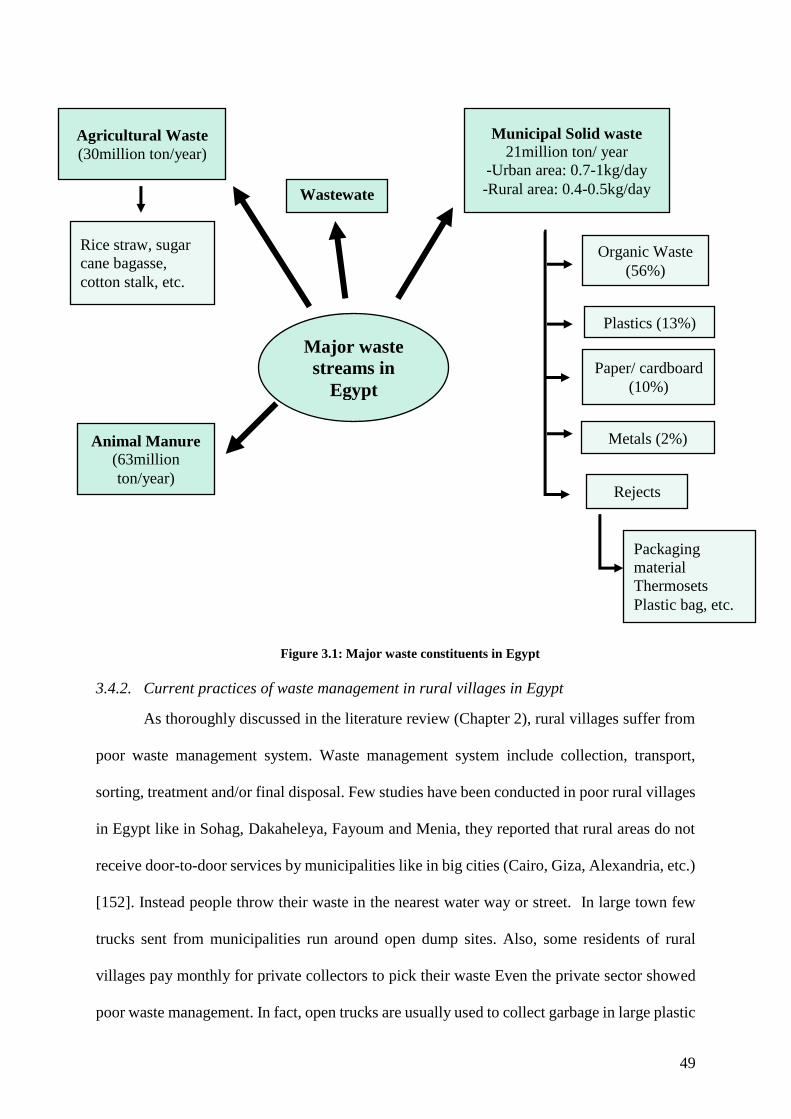
49
Figure 3.1: Major waste constituents in Egypt
3.4.2. Current practices of waste management in rural villages in Egypt
As thoroughly discussed in the literature review (Chapter 2), rural villages suffer from
poor waste management system. Waste management system include collection, transport,
sorting, treatment and/or final disposal. Few studies have been conducted in poor rural villages
in Egypt like in Sohag, Dakaheleya, Fayoum and Menia, they reported that rural areas do not
receive door-to-door services by municipalities like in big cities (Cairo, Giza, Alexandria, etc.)
[152]. Instead people throw their waste in the nearest water way or street. In large town few
trucks sent from municipalities run around open dump sites. Also, some residents of rural
villages pay monthly for private collectors to pick their waste Even the private sector showed
poor waste management. In fact, open trucks are usually used to collect garbage in large plastic
Wastewate
r
Animal Manure
(63million
ton/year)
Agricultural Waste
(30million ton/year)
Rice straw, sugar
cane bagasse,
cotton stalk, etc.
Municipal Solid waste
21million ton/ year
-Urban area: 0.7-1kg/day
-Rural area: 0.4-0.5kg/day
Organic Waste
(56%)
Plastics (13%)
Metals (2%)
Rejects
Paper/ cardboard
(10%)
Packaging
material
Thermosets
Plastic bag, etc.
Major waste
streams in
Egypt
50
bags causing spreading of bad odor in the village and leakage of leachate from plastic bags and
truck. Therefore, people tend to throw their waste in the nearest water way or open dump site
or burn them in the street causing many environmental problems. Very few percentage of waste
is landfilled, according to the country report of waste only 7% of MSW generated in Egypt is
landfilled. There is no accurate data on the percentage of landfilled solid waste in rural areas.
Yet, El Messery et. al [34] evaluated the waste management system in 143 rural villages and
concluded that only 27% of waste generated in these villages are collected and transferred to
landfills. The study also revealed that these landfills are not well designed and constructed nor
well operated, they resemble more to open dump sites. Similar results were reported in the
annual report of the Ministry of State for Environmental Affairs [153]. This can lead to
pollution of surface and ground water as well as many other environmental problems related
to burning of solid waste. Also, only 7% of the MSW is composted and 10-15% recycled and
the rest end up in open dump sites [11].
In rural villages waste is usually re-used or recycled on a household level. In fact, in
Fayoum for example it was reported that plastics and glass bottles are re-used for storage
purposes in households and also families recycle the organic matter and use it as animal fodder
[153]. Also, in some areas there are waste dealers that buy recyclable waste such as plastics,
glass, metals and papers. The rest of the waste is perceived as being unrecyclable or have no
value.
3.4.3. Problems associated with waste management in rural villages in Egypt
The literature presented in the previous sections as well as in Chapter 2 reveals that the
major problems associated with waste management in rural villages in Egypt are as follows:
Population growth leading to generation of huge amounts of wastes
Three major problems facing rural villages:
o Generation of huge amounts of organic waste
51
o Generation of huge amounts of MSW
o Presence of waste that is perceived as impossible or hard to recycle are left in
open dump site and streets
High cost of traditional waste disposal methods (incineration and landfilling) causing
huge burden on municipalities and farmers in rural areas causing the following:
o Lack of collection services in small rural villages
o Available landfills are not well designed and constructed and resemble more to
open dump sites
As an easy and cheap solution, residents of rural villages tend to throw their waste in
the nearest water way and open dump site or burn them in the streets
Most of the missing wastes in dumpsites, streets and water ways are perceived as being
unrecyclable and of no value
3.5. Pathway to Sustainable Rural Communities in Egypt
3.5.1. Sustainable Strategies in industrial sector
The development of the concept of sustainability raised the awareness of people on the
importance of conservation of natural resources. This concept has been widely implemented in
industrial sector as thoroughly presented in chapter 2. The following concepts have been
developed and implemented in many countries reach sustainable industrial community. The
first concept is cradle-to-cradle (C2C) that aims to move towards a cyclical flow of material in
which goods are made of material that can be recycled an infinite number of time. The second
concept is Industrial Ecology (IE) from which many Eco-Industrial Parks (EIP) has been
implemented. The third concept is Environmentally Balanced Industrial Complex (EBIC), in
which compatible industries are grouped in one area to facilitate the use and transportation of
waste among different industries. The main advantage of adopting these concepts is to
minimize and/or eliminate the cost of raw material, transportation, storage, and waste disposal

52
and treatment. Unfortunately, limited number of studies focused on developing concept that
can allow full utilization of waste generated in rural villages and reach sustainable rural
communities.
3.5.2. Plans and strategies for waste management in Egypt
The government of Egypt is aiming to achieve sustainable development to improve
people’s living conditions. In 2016, the government of Egypt launched its Sustainable
Development Strategy: Egypt Vision 2030, which frames the government’s actions for the next
15 years and acts as its long-term development strategy covering the three development
dimensions; economic, social, and environmental. The main goal of the Egyptian government
is to “end all forms of poverty, fight inequalities, and tackle climate change, while ensuring
that no one is left behind” [5].
Egypt has launched its SDGs: Egypt: Vision 2030 as it is committed towards achieving
the United Nations Sustainable Development Goals (SDGs), which includes a set of 17
Sustainable Development Goals (SDGs) to end poverty, fight inequality and injustice, and
tackle climate change by 2030.
Rural villages in Egypt have been marginalized for a long time pretending that these
areas are isolated and far away from urban cities and does not have any impact on urban
prosperity. However, millions of people are living in these areas and suffer from serious
environmental problems that caused many economic and social challenges. As illustrated in
Figure 3.2, one way to develop Sustainable Rural Communities and contribute to UN and
Egyptian Sustainable Development Goals is to introduce and implement concepts used in
industrial sector.
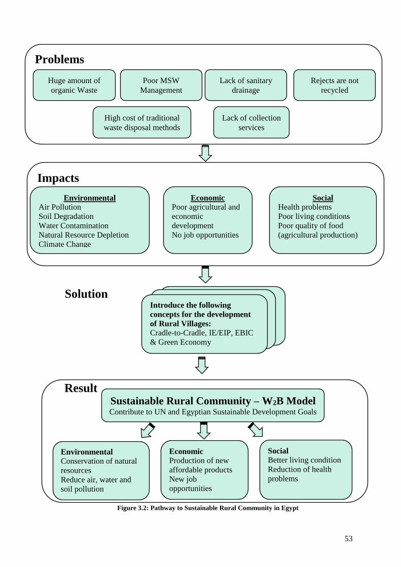
53
Figure 3.2: Pathway to Sustainable Rural Community in Egypt
Problems
Huge amount of
organic Waste
Poor MSW
Management
Lack of sanitary
drainage
Rejects are not
recycled
Impacts
Environmental
Air Pollution
Soil Degradation
Water Contamination
Natural Resource Depletion
Climate Change
Economic
Poor agricultural and
economic
development
No job opportunities
Social
Health problems
Poor living conditions
Poor quality of food
(agricultural production)
Solution
Introduce the following
concepts for the development
of Rural Villages:
Cradle-to-Cradle, IE/EIP, EBIC
& Green Economy
Result Sustainable Rural Community – W2B Model Contribute to UN and Egyptian Sustainable Development Goals
High cost of traditional
waste disposal methods
Lack of collection
services
Environmental
Conservation of natural
resources
Reduce air, water and
soil pollution
Economic
Production of new
affordable products
New job
opportunities
Social
Better living condition
Reduction of health
problems
54
3.6. Proposed Waste to Business Model (W2B) for Rural Communities
Rural villages in Egypt have always been neglected and marginalized and always
perceived as isolated areas. Yet, these areas are home to a large portion of the Egyptian
population, which are confronted with many environmental, economic and social problems that
cannot be ignored anymore. Resident of rural communities suffer from pverty and poor waste
management systems, which make them live at high risk for diseases in informal houses,
drinking and eating polluted water and food. The best solution to solve these problems is to
develop a concept similar to the ones developed in the industrial sector that will allow to
alleviate the environmental, economic and social problems facing these areas.
The Waste to Business Model (W2B) consists of developing in each rural village a
facility that groups small and affordable technologies to recycle all types of wastes generated
from rural this village. This facility will receive all types of waste generated from the rural
village, naming, agricultural waste – municipal solid waste, wastewater, as a source of raw
material – and distribute them among the following four main units including (1) animal fodder
unit, (2) biogas unit, and (3) composting/ organic fertilizer unit, (4) recycling of municipal solid
waste unit. The idea of this facility is illustrated in Figure 3.3. This waste will; thus, be used
to produce organic fertilizer, bio-energy, animal fodder and other products according to the
market need.
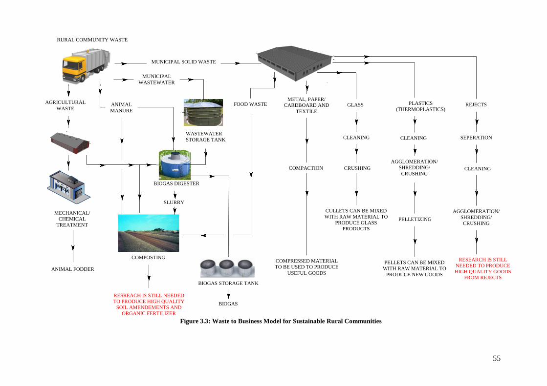
55
Figure 3.3: Waste to Business Model for Sustainable Rural Communities
FOOD WASTE REJECTS
SEPERATION
AGGLOMERATION/
SHREDDING/
CRUSHING
RESEARCH IS STILL
NEEDED TO PRODUCE
HIGH QUALITY GOODS FROM REJECTS
PLASTICS
(THERMOPLASTICS)
CLEANING
AGGLOMERATION/ SHREDDING/
CRUSHING
PELLETIZING
PELLETS CAN BE MIXED
WITH RAW MATERIAL TO
PRODUCE NEW GOODS
GLASS
CLEANING
CRUSHING
CULLETS CAN BE MIXED
WITH RAW MATERIAL TO
PRODUCE GLASS PRODUCTS
METAL, PAPER/ CARDBOARD AND
TEXTILE
COMPACTION
COMPRESSED MATERIAL
TO BE USED TO PRODUCE
USEFUL GOODS
RURAL COMMUNITY WASTE
ANIMAL FODDER
MECHANICAL/
CHEMICAL
TREATMENT
AGRICULTURAL
WASTE
MUNICIPAL SOLID WASTE
MUNICIPAL
WASTEWATER
WASTEWATER
STORAGE TANK
BIOGAS DIGESTER
SLURRY
BIOGAS STORAGE TANK
BIOGAS
COMPOSTING
RESREACH IS STILL NEEDED
TO PRODUCE HIGH QUALITY SOIL AMENDEMENTS AND
ORGANIC FERTILIZER
ANIMAL
MANURE
CLEANING
56
Composting/Organic fertilizer
As thoroughly discussed in chapter 2, composting is a process in which optimum
environment are settled (moisture content and oxygen) for aerobic bacteria to decompose
organic matter and produce soil amendment and/ or organic fertilizer. There are several
methods for composting process. In rural areas, it is recommended to use natural composting
method that require manual turning of piles as it is a cheap technique that does not require high
capital cost. This method requires lot of workers, which is an advantage in rural areas as they
people suffer from unemployment. Using organic fertilizer and/or soil amendment made from
composting of organic waste is advantageous as it will improve the soil structure and eliminate
the pollution caused by burning of waste. Other additives can be inoculated to the compost pile
such as natural rocks (phosphate - source of phosphorus, feldspar - source of potassium,
dolomite - source of magnesium, etc.) to produce organic fertilizer for organic farming, which
can replace expensive imported chemical fertilizers [6]. However, composting is not widely
practiced in developing countries because it is time consuming and quality of product received
can be unstable. More research is required to understand the process more and increase the
quality of compost and/or organic fertilizer produced.
Animal Fodder
Animal foodstuff is not available in large quantities in the local market in many rural
villages in Egypt. Rather, animal foodstuff is imported to fill the gap in the market at relatively
high cost. Hence, several research is done to produce animal foodstuff from agricultural waste
to overcome this deficiency.
The size and toughness of many agricultural wastes makes it hard for animals to
consume them directly. They need to be mechanically or chemically treated first. [154]. The
mechanical treatment consists of reducing the size of agricultural waste via chopping,
shredding and grinding. Then the waste is soaked in water to soften it, and finally is streamed
57
under pressure. However, this mechanical method requires several equipment that consume
energy which make it relatively expensive and thus prevent its spread.
Another method consists of mixing agricultural waste with urea or ammonia. The mix
is covered with covered with a 2mm thick polyethylene wrapping material for 2 weeks in
summer and 3 weeks in winter. Then the cover is removed, and the mix is left for 2 to 3 days
to release remaining ammonia before being used [154]. . This method was reported to be
feasible and produce high quality animal fodder [14, 154, 155].
Biogas
Many rural villages suffer from incessant power outage; therefore, they meet their
energy needs via traditional energy sources including firewood, dung and crop residues. These
traditional methods are often expensive and/or time-consuming [6]. On the other hand, huge
amount of organic waste is generated every year such as agricultural waste, food waste from
MSW, wastewater, animal manure and animal residues. These wastes are left in the streets,
open dump sites and water canals causing extensive pollution. Many research indicated that
these wastes are organic carbon-based material that are subject to natural anaerobic
degradation when left and release from 590 to 800 million tons of methane in the atmosphere
[156]. In other words, if these wastes are placed in optimum conditions for anaerobic
decomposition to take place, large amount of biogas can be produced and used to meet the
energy needs of the rural population instead of using natural resources.
To produce biogas, organic material is placed in a container in the absence of oxygen for
anaerobic bacteria to grow and consume organic matter to produce a mixture of methane and
carbon dioxide. Biogas is a clean, efficient and renewable source of energy that can be used as
a substitute for natural gas in rural communities. Research has found that 1.0 m3 of purified
biogas is equivalent to 1.1 L of gasoline, 1.7 L of bioethanol, or 0.97 m3 of natural gas [157].
58
The slurry from the digester has high nutritional value and can therefore be utilized in the
composting process produce organic fertilizer.
Many countries started using biogas. For example, in China 30 million household
digesters are operating and aiming to reach 80 million by 2020. There are 162 farms scale plant
in America serving 41,000 homes. Germany has more than 4,000 farm scale digesters, Austria
has 350, United Kingdom 65 [157]. However, biogas technology is not very popular in Africa
and needs to be more researched via universities and research centers to suit different country’s
needs.
There are several types of biogas digesters including [156]:
Chinese fixed dome digester: It consists of a digester topped with a fixed (non-movable)
dome (or well) made out of concrete and usually constructed underground. Raw
material is introduced to the fermentation reservoir via a feed tank. Once gas is formed
it expands and gas is pushed out of the reservoir also the produce gas pushes the slurry
to overflow into the overflow tank to be stored. This design is easy to use and construct
as it does not have any moving parts. Yet, gas produce is not constant, so it is difficult
to use in applications where energy cannot be fluctuating.
Floating dome digester: It consists of a movable cylindrical dome shaped digester made
of stainless steel and a guiding frame to prevent the dome from tilting while moving up
and down. The dome floats up and down depending on the amount of biogas produced
in the digester. Also, the gas produced in not constant as in the case of Chinese fixed
dome digester. This design is more expensive and require more maintenance compared
to the fixed done design.
Bag digester: The Union Industrial Research Laboratories in Hsinchu, Tawian
developed the bag digester, which consists of a plastic bag digester. The reactor is made
of a mixture of PVC and red mud generated from the production of aluminum known
59
as Red Mud Plastic (RMP). There are several types of bag digester among them is the
balloon digester. In this design the digester skin is made of thin and flexible plastic
allowing for the agitation of slurry, which optimize the digestion process. Bag digesters
is recommended type of digester to be use in rural areas as it is relatively inexpensive.
However, research is still needed to fully understand how it works and increase it
efficiency.
Municipal Solid Waste (MSW)
As thoroughly discussed previously MSW is a major concern in rural communities.
Most of the MSW generated in rural villages ends up in open, public and random dumpsites
resulting into environmental, economic and social problems. Bad odors are emitted from MSW
left without proper disposal techniques. These piles of wastes dumped everywhere attract flied
and mosquitos, which put the residents of rural villages at high risk for diseases. Also, waste
leachate and waste dumped in waterways contaminate both water pass ways as well as ground
water and burning the waste releases greenhouse gases to the atmosphere, which pollute the
air.
The traditional disposal techniques including landfilling or incineration are very
expensive and contribute to depletion of natural resources. Also, the accumulation of piles of
garbage in the streets can cause social and economic impact in addition to environmental
problems. The absence of awareness of people of the size of the problem make recycling of
MSW in rural villages in Egypt challenging. Also, to solve the problem people tend to import
expensive technologies that are not suitable for the rural context of Egpt, which limit their use
and spread.
The W2B facility will receive all types of MSW generated in rural village. The waste
will be placed on a conveyor belt and manually sorted and distributed among different units.
60
Thermoplastics will first be cleaned, cut and shredded and/or agglomerated depending
on type of plastic. It will be subject to heat via extrusion machine and pelletized. The formed
pellets can then be reprocessed to form products suitable for the market need.
Glass are cleaned and crushed into small pieces called cullets, which can then be mixed
with raw material to produce new glass products, which will reduce raw material and energy
used in the production of glass.
A hydraulic press is used to compact metal, paper and cardboard and textile wastes to
be easy stored, handled and transported to recycling facilities. Ingots are formed by melting
metals that can then be used to produce new products. Also, compacted paper, cardboard and
textile can then be reprocessed to produce useful products.
Food waste can be recycled via composting as described above.
MSW also contained rejects, which are material that are perceived as hard or impossible
to recycle such as packaging material, contaminated plastic bags, thermosets, etc. Very few
research is done to recycle rejects using simple and affordable methods suitable for rural
communities. As fully discussed in Chapter 2 several expensive methods have been proposed
in the literature that cannot be implemented in rural villages, hence, it is imperative to develop
easy and cheap technologies to recycle rejects.
3.7. Conclusion
It is proposed that the government, the rural community, business community and
academic institutions and research centers collaborate to implement W2B model in rural
communities. W2B model consists of having a facility in each rural community that groups
simple and obtainable technologies to fully utilize all types of wastes generated in rural village
and produce useful products. The waste is manually sorted among different units. Wastewater
is stored in a tank and then used to produce biogas. The slurry from the biogas digester along
with agricultural waste, food waste and animal manure are used in composting process to
61
produce high quality fertilizer. Yet research is still needed to understand the effect of different
additives on the composting process and to accelerate the process. MSW is then sorted
manually and distributed among different units to produce useful goods depending on the
market need of the village. One type of MSW is reject, material that are hard to recycle, still
research is needed to fully utilize rejects to produce useful good at an affordable manner. In
other words, this facility will collect all type of wastes generated in the rural village and will
recycle them to produce useful products. By applying this approach, the village will be able to
conserve natural resources, reduce the environmental, health, economic and social problems
facing these remote areas due to burning and dumping waste. It will also help in creating new
job opportunities and reduce the cost of goods.
While reviewing different waste streams it became obvious that there are two main important
problems in rural villages in Egypt that need to be studied in depth:
Recycling of organic waste
Recycling or rejects
Therefore, the two following chapters will focus on recycling of these two types of waste as
illustrated in Figure 3.4.
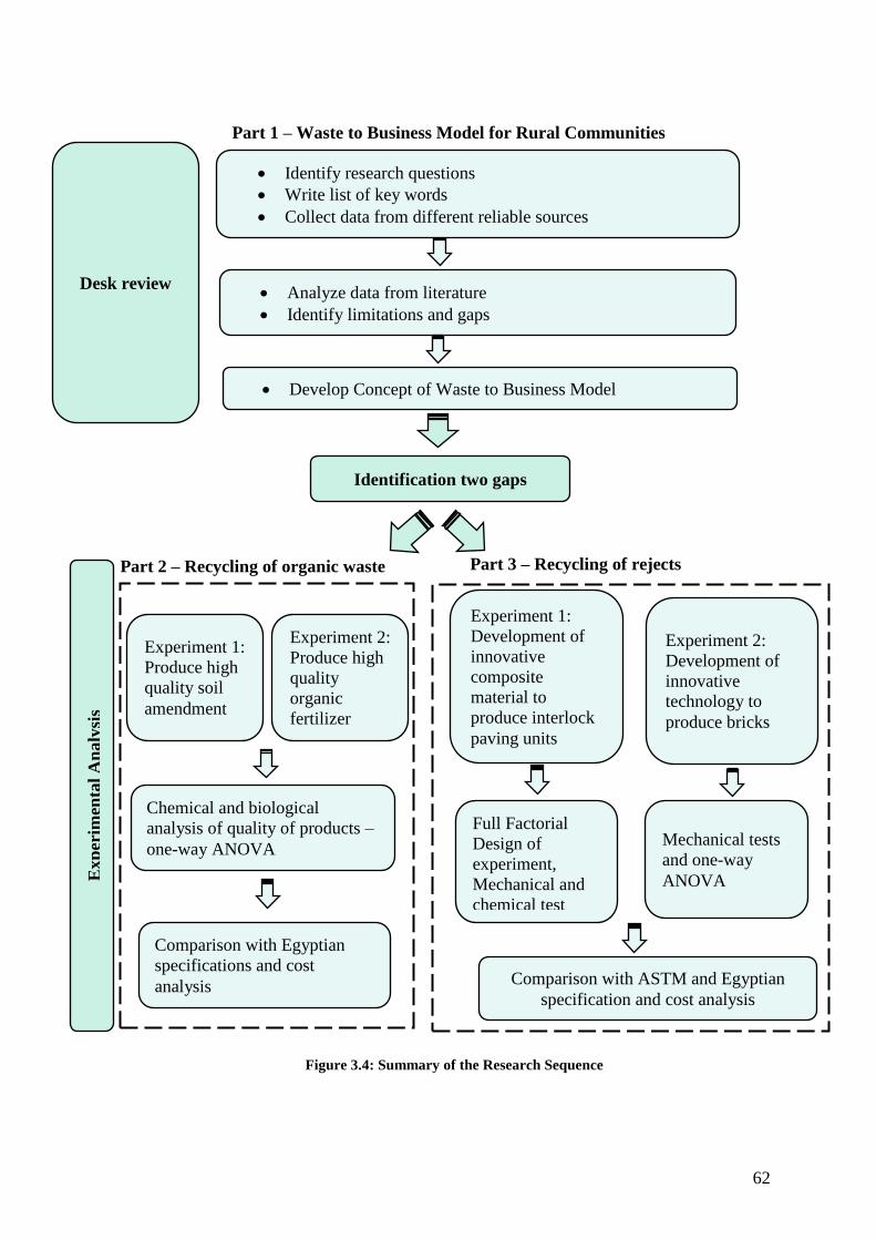
62
Figure 3.4: Summary of the Research Sequence
Desk review
Identify research questions
Write list of key words
Collect data from different reliable sources
Develop Concept of Waste to Business Model
Part 1 – Waste to Business Model for Rural Communities
Identification two gaps
Analyze data from literature
Identify limitations and gaps
Ex
per
imen
tal
An
aly
sis
Part 2 – Recycling of organic waste Part 3 – Recycling of rejects
Experiment 1:
Produce high
quality soil
amendment
Full Factorial
Design of
experiment,
Mechanical and
chemical test
Chemical and biological
analysis of quality of products –
one-way ANOVA
Comparison with ASTM and Egyptian
specification and cost analysis
Comparison with Egyptian
specifications and cost
analysis
Experiment 2:
Produce high
quality
organic
fertilizer
Experiment 1:
Development of
innovative
composite
material to
produce interlock
paving units
Experiment 2:
Development of
innovative
technology to
produce bricks
Mechanical tests
and one-way
ANOVA
63
CHAPTER 4 – SUSTAINABLE BIO-CONVERSION OF
AGRICULTURAL WASTE INTO HIGH QUALITY
ORGANIC FERTILIZER – CASE STUDY OF RICE
STRAW
As thoroughly discussed in the previous chapters huge amounts of organic wastes are
generated every year in rural areas in Egypt. There are several types of organic waste and this
research focuses on agricultural waste as a type of organic waste. Egypt generates up to 30
million ton/year of agricultural waste [12], from which 52% are directly burnt in the fields [13].
One of the main types of agricultural waste generated in Egypt is rice straw. Even after the
decision of the Ministry of Irrigation and Water Resources to reduce the amount of rice
cultivated in Egypt from 1,700,000 feddans to 724,200 feddans still this generates huge
amounts of rice straw every year in Egypt. It is estimated that around 5.9million tons of rice
straw were generated in 2013 [17]. Therefore, it could be estimated that today around
2.5million tons of rice straw are generated per year. A portion of the rice straw is mainly used
as fuel for cooking and house heating, animal feed, fiber for pulping and plowing into farmland.
A large amount of rice straw is dumped and burned in open fields causing serious
environmental problems, including air pollution and soil degradation [16, 17]. Rice straw
contains cellulose and hemicellulose and lining. Several studies showed that rice straw could
be used to produce high value-added products via microbial fermentation process [81, 82].
There is an urgent need to find efficient and cost-effective methods to reduce environmental
pollution and recycle agricultural resources.
Composting is an efficient method to transform agricultural waste into high quality soil
amendment and/or organic fertilizer and instead of degrading the soil via burring of waste in
the field, the use of organic fertilizer made of waste can rebuild the soil structure. [5, 17, 22,
71]. Thus, replace the overuse of expensive chemical fertilizer that largely contributed to
environmental deterioration. Composting is a biological process in which complex organic
64
matters are degraded by aerobic thermophilic and mesophilic microorganisms and converted
into mineralized products (CO2, H2O, ) and stabilized organic matter that can then be used as
plant nutrients [61, 63, 158]. Although composting has been widely practiced, the process is
still not fully understood due to high variety and heterogeneity of feedstocks [71]. The
objectives of composting are to accelerate and create optimum conditions for the naturally
occurring decomposition process to take place.
Composting goes through four phases: (1) mesophilic phase is a preparatory stage,
which initiates organic matter decomposition; (2) thermophilic phase in which microorganisms
decompose organic matter at high temperatures ranging from 40–70°C; (3) second mesophilic
phase allowing re-establishment of the heat resistant microbes; and (4) maturity phase of
constant nutrient contents [159].
There are several factors that affect the quality and decomposition rate of the compost,
including moisture content, temperature, oxygen, and C/N ratio [22]. Also, the inoculation of
microbial additives can tolerate composting condition, accelerate the composting process and
increase nutrients is important to study.
Some studies showed that the use of additives is a beneficial option to improve
nutritional value of compost and accelerate the degradation process [103]. Some of these
amendments include biochar, effective micro-organisms (EM), cellulose decomposing
bacteria, starters containing bacillus, fungi, yeast, lactic acid bacteria, and animal manure.
Several producers of these additives claim that they can generate higher quality compost during
short period of time. Yet, the effect of these additives on the composting process is not fully
studied and understood. The aim of these experiments is to evaluate the effect of different
additives on the quality of rice straw compost.
65
4.1. Objectives
In this part rice straw has been chosen as one type of organic waste that is present in huge
amounts in rural Egypt. The aim of this part is to produce high quality soil amendments and
organic fertilizers by composting of rice straw. This part is divided into two sets of experiments
as follows:
The objectives of the first set of experiment are to:
Transform rice straw into soil amendment or soil conditioner
Evaluate and compare the effect of different additives on the quality of produced
soil amendment
The objectives of the second set of experiment are to
Transform rice straw and animal manure into high quality organic fertilizer
Evaluate and compare the effect of different additives on quality of produced
organic fertilizer
Compare the cost of produced organic fertilizer with commercially available
chemical fertilizer
4.2. Materials and Methods
Based on the first part of this research work, it became obvious that recycling of organic
waste is still not fully understood and need to be investigated. In order to address this aim,
experimental analysis is conducted.
The aim of this part of the research work is to evaluate and compare the effect of inoculating
different types of additives on composting process. To achieve this aim two pilot scale
experiments are conducted at the American University in Cairo, Egypt to study the
bioconversion of agricultural waste into a valuable product (compost) with application of
different additives.
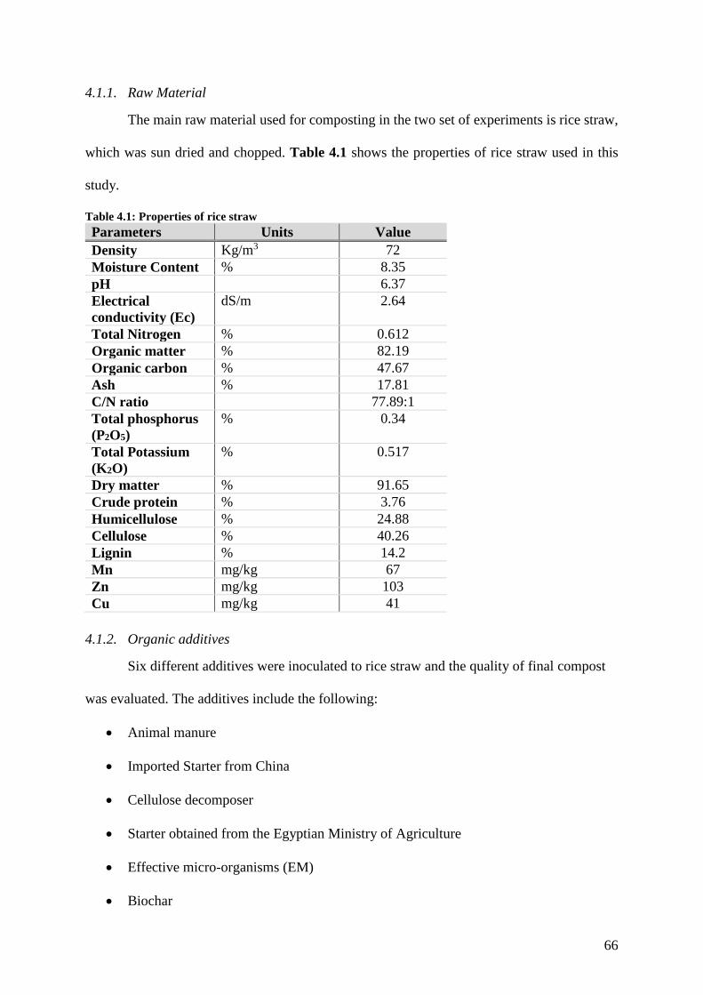
66
4.1.1. Raw Material
The main raw material used for composting in the two set of experiments is rice straw,
which was sun dried and chopped. Table 4.1 shows the properties of rice straw used in this
study.
Table 4.1: Properties of rice straw
Parameters Units Value
Density Kg/m3 72
Moisture Content % 8.35
pH 6.37
Electrical
conductivity (Ec)
dS/m 2.64
Total Nitrogen % 0.612
Organic matter % 82.19
Organic carbon % 47.67
Ash % 17.81
C/N ratio 77.89:1
Total phosphorus
(P2O5)
% 0.34
Total Potassium
(K2O)
% 0.517
Dry matter % 91.65
Crude protein % 3.76
Humicellulose % 24.88
Cellulose % 40.26
Lignin % 14.2
Mn mg/kg 67
Zn mg/kg 103
Cu mg/kg 41
4.1.2. Organic additives
Six different additives were inoculated to rice straw and the quality of final compost
was evaluated. The additives include the following:
Animal manure
Imported Starter from China
Cellulose decomposer
Starter obtained from the Egyptian Ministry of Agriculture
Effective micro-organisms (EM)
Biochar
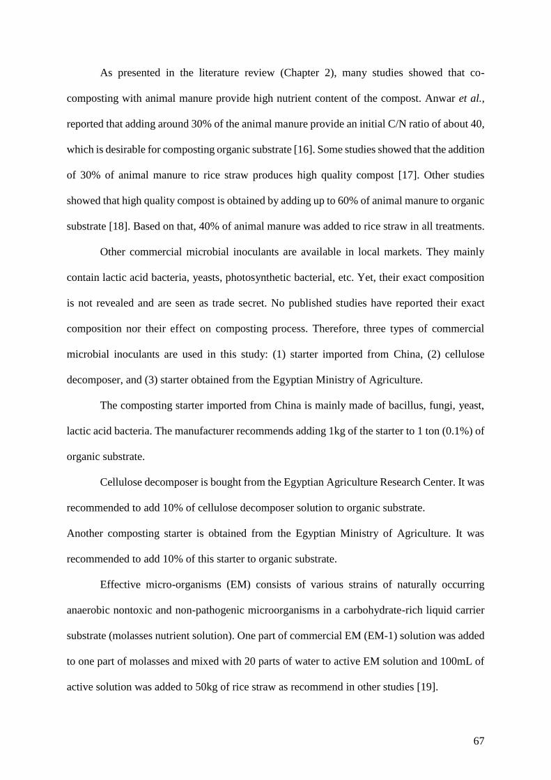
67
As presented in the literature review (Chapter 2), many studies showed that co-
composting with animal manure provide high nutrient content of the compost. Anwar et al.,
reported that adding around 30% of the animal manure provide an initial C/N ratio of about 40,
which is desirable for composting organic substrate [16]. Some studies showed that the addition
of 30% of animal manure to rice straw produces high quality compost [17]. Other studies
showed that high quality compost is obtained by adding up to 60% of animal manure to organic
substrate [18]. Based on that, 40% of animal manure was added to rice straw in all treatments.
Other commercial microbial inoculants are available in local markets. They mainly
contain lactic acid bacteria, yeasts, photosynthetic bacterial, etc. Yet, their exact composition
is not revealed and are seen as trade secret. No published studies have reported their exact
composition nor their effect on composting process. Therefore, three types of commercial
microbial inoculants are used in this study: (1) starter imported from China, (2) cellulose
decomposer, and (3) starter obtained from the Egyptian Ministry of Agriculture.
The composting starter imported from China is mainly made of bacillus, fungi, yeast,
lactic acid bacteria. The manufacturer recommends adding 1kg of the starter to 1 ton (0.1%) of
organic substrate.
Cellulose decomposer is bought from the Egyptian Agriculture Research Center. It was
recommended to add 10% of cellulose decomposer solution to organic substrate.
Another composting starter is obtained from the Egyptian Ministry of Agriculture. It was
recommended to add 10% of this starter to organic substrate.
Effective micro-organisms (EM) consists of various strains of naturally occurring
anaerobic nontoxic and non-pathogenic microorganisms in a carbohydrate-rich liquid carrier
substrate (molasses nutrient solution). One part of commercial EM (EM-1) solution was added
to one part of molasses and mixed with 20 parts of water to active EM solution and 100mL of
active solution was added to 50kg of rice straw as recommend in other studies [19].
68
Biochar is another type of additive and many studies showed that it can have a lot of
positive impacts on quality of compost. Several studies reported application of biochar with
doses from 3 to 50%. According to the literature, the recommended application dose of biochar
to compost is between 10% [39]. Some studies have also reported use of higher doses up to
50%; however, some authors have reported that doses higher than 20% can slow down the
composting process [40]. Therefore, doses of 10% and 20% are used in this study.
4.1.3. Composting procedure
Two sets of experiments are conducted. The objective of the first set of experiment is
to transform rice straw to soil conditioner. In the first set of experiments five compost piles are
constructed, each pile contains 50kg of rice straw and different activator as shown in Table
4.2. It is worth to mention that this set of experiment is conducted in winter season.
Table 4.2: Piles content used for composting process in set of experiment # 1
Treatment No. Pile Content
E1.T1 50kg of rice straw+50g of Chinese starter+1kg urea
E1.T2 50kg of rice straw+1kg of cellulose decomposer
E1.T3 50kg of rice straw+ 5kg of starter obtained from Egyptian Ministry
of Agriculture
E1.T4 50kg of rice straw+ 20kg of animal manure
E1.T5 50kg of rice straw+ 20kg of animal manure + 50g of Chinese
starter+ 1kg of urea
The objective of the second set of experiments is to transform rice straw to high quality
organic fertilizer. In the second set of experiments, nine compost piles are constructed, each
pile contained 50kg of rice straw and different activator as summarized in Table 4.3. Different
types of rocks are added at the beginning of the composting process to all treatments to enrich
the compost nutritional value. Previous study conducted at the American University in Cairo
revealed that the addition of different types of rocks to the compost with the percentages
69
presented in Table 4.4 enriches the nutrition value of final compost product [5]. It is important
to mention that this set of experiment was conducted in summer season.
Table 4.3: Piles content used for composting process in set of experiment # 2
Treatment No. Pile Content
E2.T1 50kg of rice straw+20kg of animal manure+ Mixture of Rocks
E2.T2 50kg of rice straw+20kg of animal manure + 50g of Chinese
starter+ Mixture of Rocks
E2.T3 50kg of rice straw+ 20kg of animal manure +1L of activated EM +
Mixture of Rocks
E2.T4 50kg of rice straw+ 20kg of animal manure + 5kg biochar (10%) +
Mixture of Rocks
E2.T5 50kg of rice straw+ 20kg of animal manure + 50g of Chinese
starter + 5kg of biochar (10%) + Mixture of Rocks
E2.T6 50kg of rice straw+ 20kg of animal manure + 1L of activated EM+
5kg of biochar (10%) + Mixture of Rocks
E2.T7 50kg of rice straw+ 20kg of cow manure + 10kg of biochar (20%)
+ Mixture of Rocks
E2.T8 50kg of rice straw+ 20kg of animal manure + 50g of Chinese
starter + 10kg of biochar (20%) + Mixture of Rocks
E2.T9 50kg of rice straw+ 20kg of animal manure + 1L of activated EM +
10kg of biochar (20%) + Mixture of Rocks
Table 4.4: Types of rocks used and their corresponding quantities
Type of rock Percentage
(%)
Quantity
(kg)
Value Added
Rock phosphate 2.5% 1.25 Source of Phosphorous
Feldspar 2.5% 1.25 Source of Potassium
Sulfur 2.5% 1.25 Natural Pesticide
Dolomite 2.5% 1.25 Source of magnesium and calcium
Bentonite 10% 5kg Source of Magnesium, calcium,
potassium, and iron
In both sets of experiments, the treatments are composted aerobically in large fabric
bags with aeration through turning. The moisture content is kept at around 60% in all piles by
adding water. The materials in each pile were manually turned every week. Figure 4.1
summarizes the composting process. Ambient temperature and treatments temperature were
70
measured three times a week through the center of the compost piles at different locations using
a digital thermometer. The treatments are left three months for composting. Three
homogenized and randomized samples are taken manually after 10 days, 30 days. 60 days and
90 days from top, middle and bottom of compost piles.
Figure 4.1: Summary of composting process
4.1.4. Measured Parameters
All the samples are tested as per the Egyptian Specification for Compost for the year
2017 [160] to be analyzed for the following physical, chemical and biological parameters at
the Soil, Water and Environment Research Institute, Agriculture Research Center:
Organic Matter (%OM) is the difference between ash and dry weight. The weight of
dry sample is measured. Then the sample is burnt in a furnace at 750C for 4 hours and
the weight of formed ash is measured.
Organic carbon (%OC): Van Bermmelem factor of 1.7241 is used to calculated %OC
from %OM [161],
Step 3: Piles were turned and water added every week
Step 1: 50kg of rice straw in
large fabric bags Step 2: Additive is added to pile
The treatments were left three months
Step 3: Piles are turned, and water
added every week
71
Total nitrogen, ammonium nitrogen and nitrate nitrogen: Kjeldahl method is used
to analyze the total nitrogen [154]. The sulfuric acid is added to the sample and heated
which decomposes the organic substance by oxidation to liberate the reduced nitrogen.
Ammonium nitrogen is extracted 2N KCl, then estimated by the steam distillation
Kjeltic method in alkaline media [155].
C/N ratio is calculated by dividing %organic carbon with %total nitrogen.
Moisture content and bulk density: to measure the moisture content the sample is
dried at a temperature of 105C until the weight becomes constant. The bulk density of
compost is calculated by dividing the weight of the sample by its unit volume
pH and electrical conductivity (EC): Stirred 5 g of the sample in 50 ml distilled water.
The pH value is measured using a pH digital meter with a glass electrode. The EC is
measured using EC meter.
Germination index (GI): The sample is shacked with distilled water for 1 h, and then
filtered to be used for germination of Eruca sativa seeds using Petri dishes. Seed
germination in distilled water was used as control. The percentage of seed germination
(GI) is then calculated using the following equation [162]:
GI(%) =No. of seeds germinated in compost extract
No. of seeds germinated in controlx100
Humification index (HI):
First, compost sample is mixed with a solution NaOH/Na4P2O7 0.1 N for 48 h at 65 °C. Samples
were centrifuged at 2500 rpm and supernatant solution filtered through a 0.45 μm Millipore
filter. Extracts were stored at 4 °C under nitrogen atmosphere.
Then, the extract is acidified with H2SO4 to separate humic-like acids (HA) (precipitated) from
fulvic-like acids (FA) (in solution). HA and FA are then purified on a polyvynilpyrrolidone
(PVP) column, resolubilised with NaOH and then joined to the humic portion. Combined
fractions (HA+FA) were quantitatively transferred into a calibrated 50-ml flask, brought to
72
volume with NaOH and stored at 4°C under nitrogen atmosphere. Total organic carbon in
compost samples, total extractable carbon and humic and fulvic acids carbon (HA+FA) as
proposed by Ciavatta et al. [156]. Then the Humification Index is calculated using the
following equation:
HI(%) =𝑛𝑜𝑛ℎ𝑢𝑚𝑖𝑓𝑖𝑒𝑑 𝑓𝑟𝑎𝑐𝑡𝑖𝑜𝑛 (𝑁𝐻)
HA + FAx100
Pathogenic bacteria (Total Coliform, Fecal Coliform, Salmonella and Shigella):
Pathogenic bacterial count was determined using agar plates containing specific media
for coliform group, Escherichia coli, Salmonella and Shigella.
Total Phosphorous (TP) and Total Potassium (TK): Total phosphorous is measured
calorimetrically according to the methods described by Snell and Snell [157]. Total
potassium was determined in the digested solution by flame photometer.
The objective of each measured parameter is summarized in Table 4.5
Table 4.5: Summary of measured parameters
Parameter Objective
Organic Matter
(%OM)
Measure of amount of OM and OC present in compost pile at
different stages of composting process. OM and OC are consumed by
micro-organisms during composting process. Thus, the analysis of
%OM and %OC give an indication of the activity level of micro-
organisms.
Organic Carbon
(%OC)
Total Nitrogen,
ammonium nitrogen
and nitrate nitrogen
Total nitrogen, ammonium nitrogen and nitrate nitrogen are used as
maturity index for composting.
C/N ratio C/N ratio is used as a measure of maturity level, compost stability
and indicates nitrogen availability in compost pile.
Moisture content Gives an indication that composting process has been conducted
using proper conditions.
Bulk density Gives an indication about the weight of solid material in the volume
of compost.
pH pH is measured to indicate that the compost is suitable to be used for
plants. pH is a measure of acidity in the feedstock or compost.
Ideal pH depends on compost use. A neutral pH is suitable for most
applications.
Electric conductivity
(EC)
EC is measured to indicate that the compost is tolerable by plants.
Soluble salts are determined by measuring EC. High salinity may be
toxic to plants. Ideal soluble salt levels will depend on the end use of
the compost.
73
Germination Index Measure the toxicity level of compost.
Humification Index Measure the maturity level of compost.
Pathogenic bacteria Measure the presence of harmful bacterial in compost piles.
Total phosphorus
and total potassium
Phosphorus (P) and potassium (K) are plant macronutrients. These
results provide an indication of the nutrient value of the compost
sample.
4.1.5. Statistical Analysis
All results are presented as the average of three replicates, and the means among different
treatments are compared using one-way ANOVA using SPPS version 23. The null hypothesis
states that the population means are all equal. A significance level α =0.05 is used. The
statistical results are presented in the Appendix.
4.3. Results and discussion
4.3.1. Bioconversion of organic waste into soil amendment
Temperature changes of Experiment # 1
The temperature changes for the first set of compost piles and the corresponding
ambient temperatures were recorded and summarized in Figure 4.2. The temperatures were
measured three times a week through the center of the compost piles at different locations using
a digital thermometer. The full data are presented in the Appendix. It is important to note that
the composting process was conducted during winter season. The ambient temperature
variations throughout the composting period varied between 14°C and 22°C. An increase in
piles temperatures was observed right after composting started.
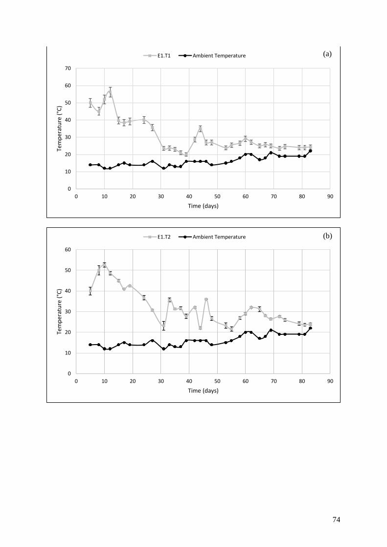
74
0
10
20
30
40
50
60
70
0 10 20 30 40 50 60 70 80 90
Tem
per
atu
re (
°C)
Time (days)
E1.T1 Ambient Temperature
0
10
20
30
40
50
60
0 10 20 30 40 50 60 70 80 90
Tem
per
atu
re (
°C)
Time (days)
E1.T2 Ambient Temperature
(a)
(b)
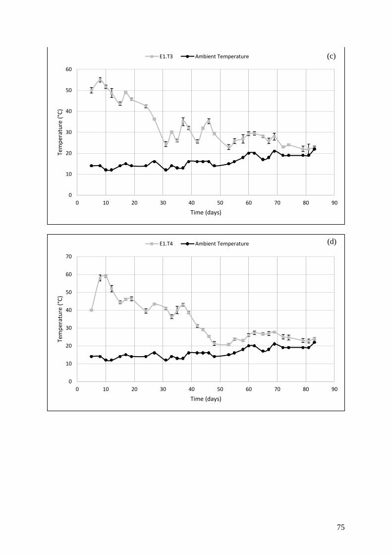
75
0
10
20
30
40
50
60
0 10 20 30 40 50 60 70 80 90
Tem
per
atu
re (
°C)
Time (days)
E1.T3 Ambient Temperature
0
10
20
30
40
50
60
70
0 10 20 30 40 50 60 70 80 90
Tem
per
atu
re (
°C)
Time (days)
E1.T4 Ambient Temperature
(c)
(d)
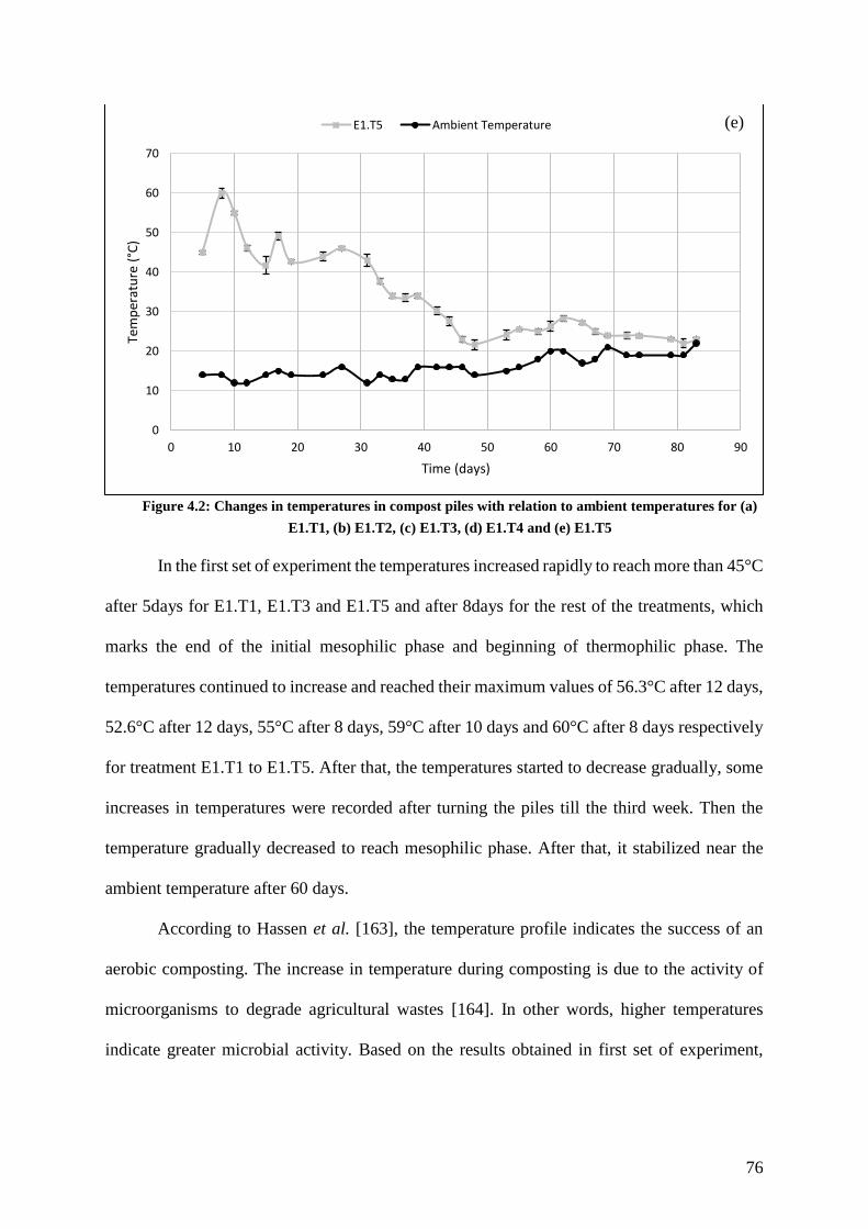
76
Figure 4.2: Changes in temperatures in compost piles with relation to ambient temperatures for (a)
E1.T1, (b) E1.T2, (c) E1.T3, (d) E1.T4 and (e) E1.T5
In the first set of experiment the temperatures increased rapidly to reach more than 45°C
after 5days for E1.T1, E1.T3 and E1.T5 and after 8days for the rest of the treatments, which
marks the end of the initial mesophilic phase and beginning of thermophilic phase. The
temperatures continued to increase and reached their maximum values of 56.3°C after 12 days,
52.6°C after 12 days, 55°C after 8 days, 59°C after 10 days and 60°C after 8 days respectively
for treatment E1.T1 to E1.T5. After that, the temperatures started to decrease gradually, some
increases in temperatures were recorded after turning the piles till the third week. Then the
temperature gradually decreased to reach mesophilic phase. After that, it stabilized near the
ambient temperature after 60 days.
According to Hassen et al. [163], the temperature profile indicates the success of an
aerobic composting. The increase in temperature during composting is due to the activity of
microorganisms to degrade agricultural wastes [164]. In other words, higher temperatures
indicate greater microbial activity. Based on the results obtained in first set of experiment,
0
10
20
30
40
50
60
70
0 10 20 30 40 50 60 70 80 90
Tem
per
atu
re (
°C)
Time (days)
E1.T5 Ambient Temperature (e)
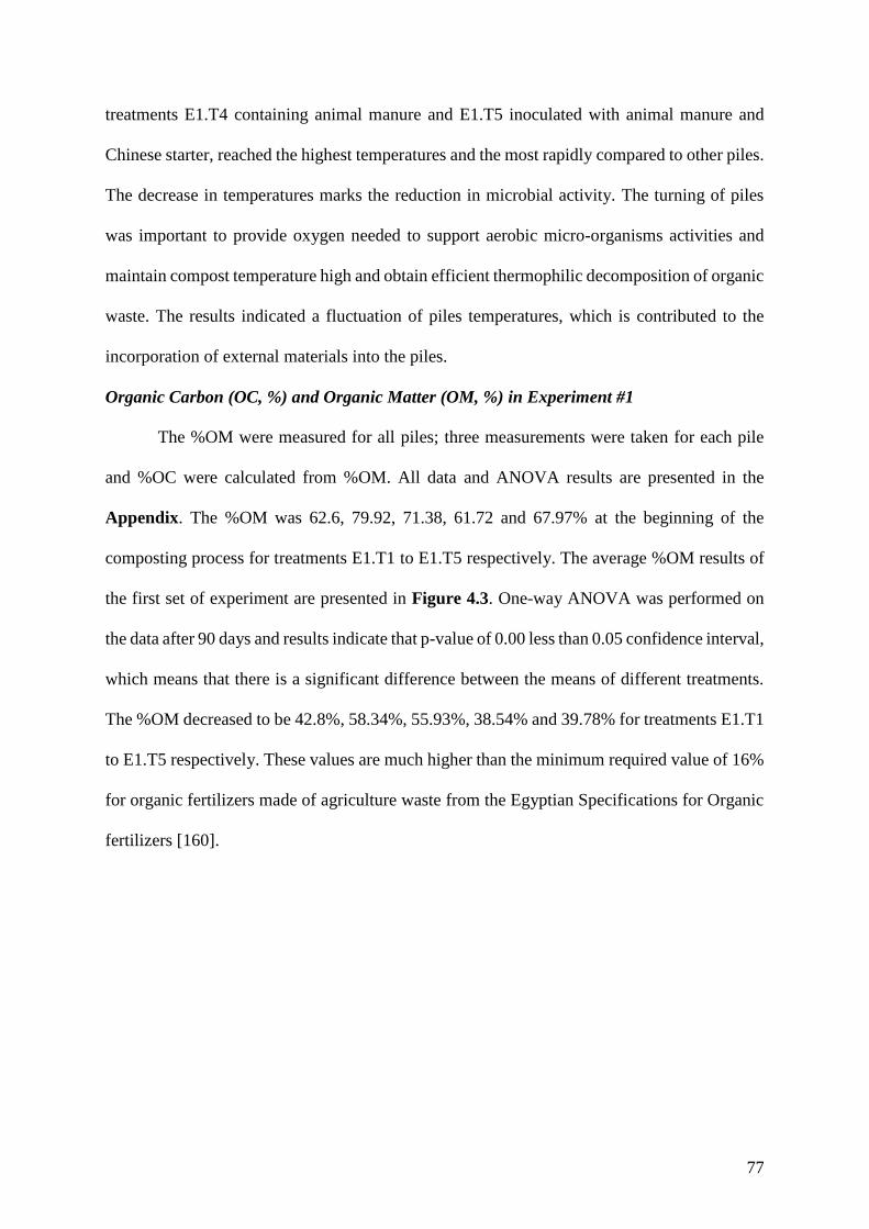
77
treatments E1.T4 containing animal manure and E1.T5 inoculated with animal manure and
Chinese starter, reached the highest temperatures and the most rapidly compared to other piles.
The decrease in temperatures marks the reduction in microbial activity. The turning of piles
was important to provide oxygen needed to support aerobic micro-organisms activities and
maintain compost temperature high and obtain efficient thermophilic decomposition of organic
waste. The results indicated a fluctuation of piles temperatures, which is contributed to the
incorporation of external materials into the piles.
Organic Carbon (OC, %) and Organic Matter (OM, %) in Experiment #1
The %OM were measured for all piles; three measurements were taken for each pile
and %OC were calculated from %OM. All data and ANOVA results are presented in the
Appendix. The %OM was 62.6, 79.92, 71.38, 61.72 and 67.97% at the beginning of the
composting process for treatments E1.T1 to E1.T5 respectively. The average %OM results of
the first set of experiment are presented in Figure 4.3. One-way ANOVA was performed on
the data after 90 days and results indicate that p-value of 0.00 less than 0.05 confidence interval,
which means that there is a significant difference between the means of different treatments.
The %OM decreased to be 42.8%, 58.34%, 55.93%, 38.54% and 39.78% for treatments E1.T1
to E1.T5 respectively. These values are much higher than the minimum required value of 16%
for organic fertilizers made of agriculture waste from the Egyptian Specifications for Organic
fertilizers [160].
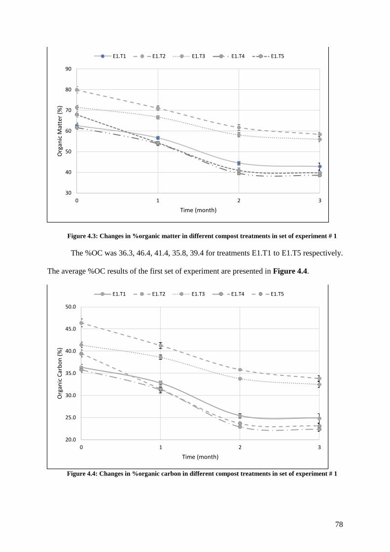
78
Figure 4.3: Changes in %organic matter in different compost treatments in set of experiment # 1
The %OC was 36.3, 46.4, 41.4, 35.8, 39.4 for treatments E1.T1 to E1.T5 respectively.
The average %OC results of the first set of experiment are presented in Figure 4.4.
Figure 4.4: Changes in %organic carbon in different compost treatments in set of experiment # 1
30
40
50
60
70
80
90
0 1 2 3
Org
anic
Mat
ter
(%)
Time (month)
E1.T1 E1.T2 E1.T3 E1.T4 E1.T5
20.0
25.0
30.0
35.0
40.0
45.0
50.0
0 1 2 3
Org
anic
Car
bo
n (
%)
Time (month)
E1.T1 E1.T2 E1.T3 E1.T4 E1.T5
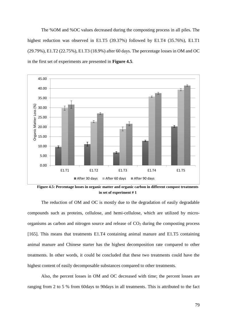
79
The %OM and %OC values decreased during the composting process in all piles. The
highest reduction was observed in E1.T5 (39.37%) followed by E1.T4 (35.76%), E1.T1
(29.79%), E1.T2 (22.75%), E1.T3 (18.9%) after 60 days. The percentage losses in OM and OC
in the first set of experiments are presented in Figure 4.5.
Figure 4.5: Percentage losses in organic matter and organic carbon in different compost treatments
in set of experiment # 1
The reduction of OM and OC is mostly due to the degradation of easily degradable
compounds such as proteins, cellulose, and hemi-cellulose, which are utilized by micro-
organisms as carbon and nitrogen source and release of CO2 during the composting process
[165]. This means that treatments E1.T4 containing animal manure and E1.T5 containing
animal manure and Chinese starter has the highest decomposition rate compared to other
treatments. In other words, it could be concluded that these two treatments could have the
highest content of easily decomposable substances compared to other treatments.
Also, the percent losses in OM and OC decreased with time; the percent losses are
ranging from 2 to 5 % from 60days to 90days in all treatments. This is attributed to the fact
0.00
5.00
10.00
15.00
20.00
25.00
30.00
35.00
40.00
45.00
E1.T1 E1.T2 E1.T3 E1.T4 E1.T5
Org
anic
Mat
ter
Loss
(%
)
After 30 days After 60 days After 90 days
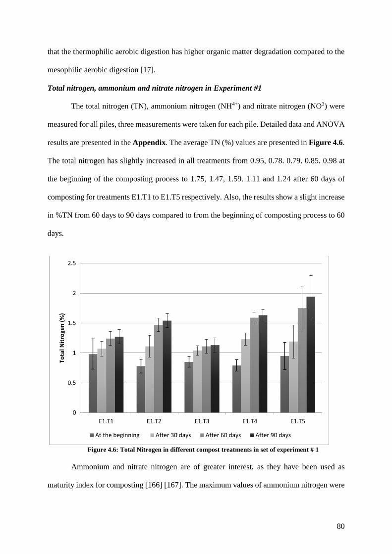
80
that the thermophilic aerobic digestion has higher organic matter degradation compared to the
mesophilic aerobic digestion [17].
Total nitrogen, ammonium and nitrate nitrogen in Experiment #1
The total nitrogen (TN), ammonium nitrogen (NH4+) and nitrate nitrogen (NO3) were
measured for all piles, three measurements were taken for each pile. Detailed data and ANOVA
results are presented in the Appendix. The average TN (%) values are presented in Figure 4.6.
The total nitrogen has slightly increased in all treatments from 0.95, 0.78. 0.79. 0.85. 0.98 at
the beginning of the composting process to 1.75, 1.47, 1.59. 1.11 and 1.24 after 60 days of
composting for treatments E1.T1 to E1.T5 respectively. Also, the results show a slight increase
in %TN from 60 days to 90 days compared to from the beginning of composting process to 60
days.
Figure 4.6: Total Nitrogen in different compost treatments in set of experiment # 1
Ammonium and nitrate nitrogen are of greater interest, as they have been used as
maturity index for composting [166] [167]. The maximum values of ammonium nitrogen were
0
0.5
1
1.5
2
2.5
E1.T1 E1.T2 E1.T3 E1.T4 E1.T5
Tota
l Nit
roge
n (
%)
At the beginning After 30 days After 60 days After 90 days
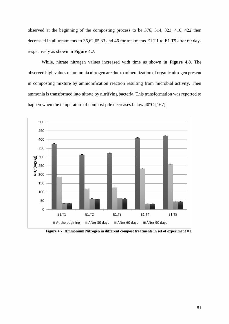
81
observed at the beginning of the composting process to be 376, 314, 323, 410, 422 then
decreased in all treatments to 36,62,65,33 and 46 for treatments E1.T1 to E1.T5 after 60 days
respectively as shown in Figure 4.7.
While, nitrate nitrogen values increased with time as shown in Figure 4.8. The
observed high values of ammonia nitrogen are due to mineralization of organic nitrogen present
in composting mixture by ammonification reaction resulting from microbial activity. Then
ammonia is transformed into nitrate by nitrifying bacteria. This transformation was reported to
happen when the temperature of compost pile decreases below 40°C [167].
Figure 4.7: Ammonium Nitrogen in different compost treatments in set of experiment # 1
0
50
100
150
200
250
300
350
400
450
500
E1.T1 E1.T2 E1.T3 E1.T4 E1.T5
NH
4+(m
g/kg
)
At the begining After 30 days After 60 days After 90 days
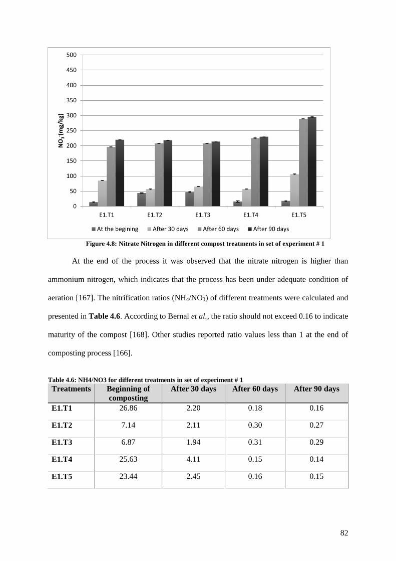
82
Figure 4.8: Nitrate Nitrogen in different compost treatments in set of experiment # 1
At the end of the process it was observed that the nitrate nitrogen is higher than
ammonium nitrogen, which indicates that the process has been under adequate condition of
aeration [167]. The nitrification ratios (NH4/NO3) of different treatments were calculated and
presented in Table 4.6. According to Bernal et al., the ratio should not exceed 0.16 to indicate
maturity of the compost [168]. Other studies reported ratio values less than 1 at the end of
composting process [166].
Table 4.6: NH4/NO3 for different treatments in set of experiment # 1
Treatments Beginning of
composting
After 30 days After 60 days After 90 days
E1.T1 26.86 2.20 0.18 0.16
E1.T2 7.14 2.11 0.30 0.27
E1.T3 6.87 1.94 0.31 0.29
E1.T4 25.63 4.11 0.15 0.14
E1.T5 23.44 2.45 0.16 0.15
0
50
100
150
200
250
300
350
400
450
500
E1.T1 E1.T2 E1.T3 E1.T4 E1.T5
NO
3- (m
g/kg
)
At the begining After 30 days After 60 days After 90 days
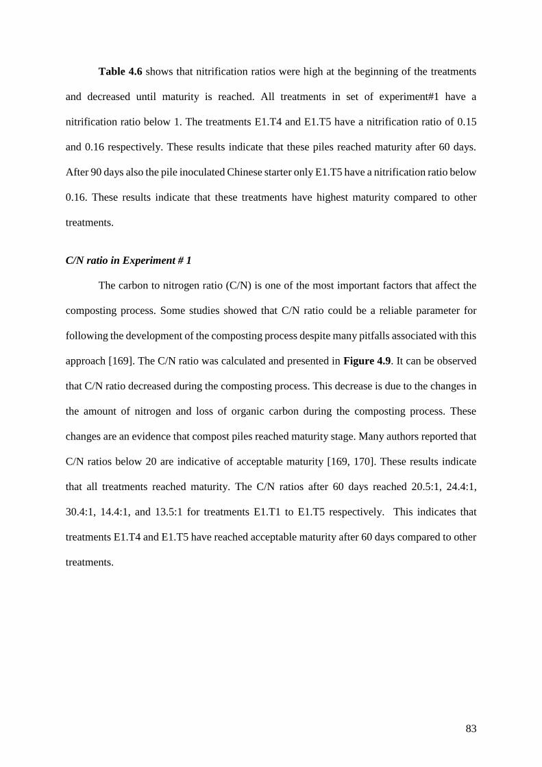
83
Table 4.6 shows that nitrification ratios were high at the beginning of the treatments
and decreased until maturity is reached. All treatments in set of experiment#1 have a
nitrification ratio below 1. The treatments E1.T4 and E1.T5 have a nitrification ratio of 0.15
and 0.16 respectively. These results indicate that these piles reached maturity after 60 days.
After 90 days also the pile inoculated Chinese starter only E1.T5 have a nitrification ratio below
0.16. These results indicate that these treatments have highest maturity compared to other
treatments.
C/N ratio in Experiment # 1
The carbon to nitrogen ratio (C/N) is one of the most important factors that affect the
composting process. Some studies showed that C/N ratio could be a reliable parameter for
following the development of the composting process despite many pitfalls associated with this
approach [169]. The C/N ratio was calculated and presented in Figure 4.9. It can be observed
that C/N ratio decreased during the composting process. This decrease is due to the changes in
the amount of nitrogen and loss of organic carbon during the composting process. These
changes are an evidence that compost piles reached maturity stage. Many authors reported that
C/N ratios below 20 are indicative of acceptable maturity [169, 170]. These results indicate
that all treatments reached maturity. The C/N ratios after 60 days reached 20.5:1, 24.4:1,
30.4:1, 14.4:1, and 13.5:1 for treatments E1.T1 to E1.T5 respectively. This indicates that
treatments E1.T4 and E1.T5 have reached acceptable maturity after 60 days compared to other
treatments.
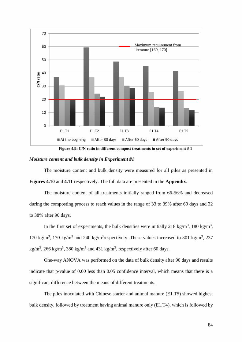
84
Figure 4.9: C/N ratio in different compost treatments in set of experiment # 1
Moisture content and bulk density in Experiment #1
The moisture content and bulk density were measured for all piles as presented in
Figures 4.10 and 4.11 respectively. The full data are presented in the Appendix.
The moisture content of all treatments initially ranged from 66-56% and decreased
during the composting process to reach values in the range of 33 to 39% after 60 days and 32
to 38% after 90 days.
In the first set of experiments, the bulk densities were initially 218 kg/m3, 180 kg/m3,
170 kg/m3, 170 kg/m3 and 240 kg/m3respectively. These values increased to 301 kg/m3, 237
kg/m3, 266 kg/m3, 380 kg/m3 and 431 kg/m3, respectively after 60 days.
One-way ANOVA was performed on the data of bulk density after 90 days and results
indicate that p-value of 0.00 less than 0.05 confidence interval, which means that there is a
significant difference between the means of different treatments.
The piles inoculated with Chinese starter and animal manure (E1.T5) showed highest
bulk density, followed by treatment having animal manure only (E1.T4), which is followed by
0
10
20
30
40
50
60
70
E1.T1 E1.T2 E1.T3 E1.T4 E1.T5
C/N
rat
io
At the begining After 30 days After 60 days After 90 days
Maximum requirement from
literature [169, 170]

85
treatment inoculated with Chinese starter only (E1.T1). High bulk density values indicate
higher level of activities in the decomposition of organic material to break down the loosely
combined raw materials into smaller pieces [17].
Figure 4.10: Moisture Content in different compost treatments in set of experiment # 1
Figure 4.11: Bulk density in different compost treatments in set of experiment # 1
0
10
20
30
40
50
60
70
80
E1.T1 E1.T2 E1.T3 E1.T4 E1.T5
Mo
istu
re C
on
ten
t (%
)
At the begining After 30 days After 60 days After 90 days
0
100
200
300
400
500
600
E1.T1 E1.T2 E1.T3 E1.T4 E1.T5
Bu
lk D
en
sity
(kg
/m3 )
At the begining After 30 days After 60 days After 90 days

86
pH and Electrical conductivity (EC) in Experiment #1
The electrical conductivity (EC) and pH of all piles were measured and shown in
Figures 4.12 and 4.13 respectively.
EC is a good indicator of the safety and suitability of compost. The EC of the finished
compost of all treatments are ranging between 2.3 to 3.12dS/m. Some studies showed that
values ranging between 2.0 to 6.0ds/m are considered tolerable by plants [171, 172].
Also, the pH values of all piles were in the recommended range of good compost (pH
8.15 – 8.62). According to Makan et al. the pH of finished compost should range from 7.5 to
8.5 [164].
Figure 4.12: Electrical Conductivity in different compost treatments in set of experiment # 1
0
1
2
3
4
5
6
E1.T1 E1.T2 E1.T3 E1.T4 E1.T5
Ele
ctri
cal C
on
du
ctiv
ity
(dS.
m-1
)
At the begining After 30 days After 60 days After 90 days
Recommended Range in literature [171, 172]
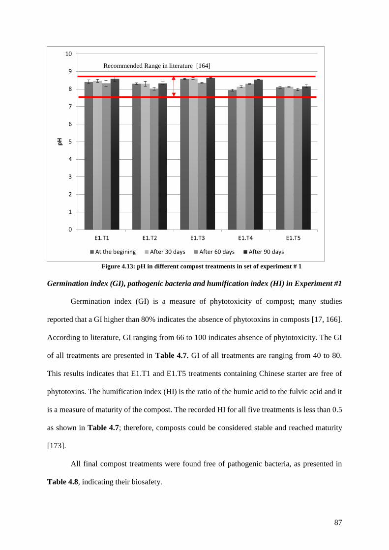
87
Figure 4.13: pH in different compost treatments in set of experiment # 1
Germination index (GI), pathogenic bacteria and humification index (HI) in Experiment #1
Germination index (GI) is a measure of phytotoxicity of compost; many studies
reported that a GI higher than 80% indicates the absence of phytotoxins in composts [17, 166].
According to literature, GI ranging from 66 to 100 indicates absence of phytotoxicity. The GI
of all treatments are presented in Table 4.7. GI of all treatments are ranging from 40 to 80.
This results indicates that E1.T1 and E1.T5 treatments containing Chinese starter are free of
phytotoxins. The humification index (HI) is the ratio of the humic acid to the fulvic acid and it
is a measure of maturity of the compost. The recorded HI for all five treatments is less than 0.5
as shown in Table 4.7; therefore, composts could be considered stable and reached maturity
[173].
All final compost treatments were found free of pathogenic bacteria, as presented in
Table 4.8, indicating their biosafety.
0
1
2
3
4
5
6
7
8
9
10
E1.T1 E1.T2 E1.T3 E1.T4 E1.T5
pH
At the begining After 30 days After 60 days After 90 days
Recommended Range in literature [164]
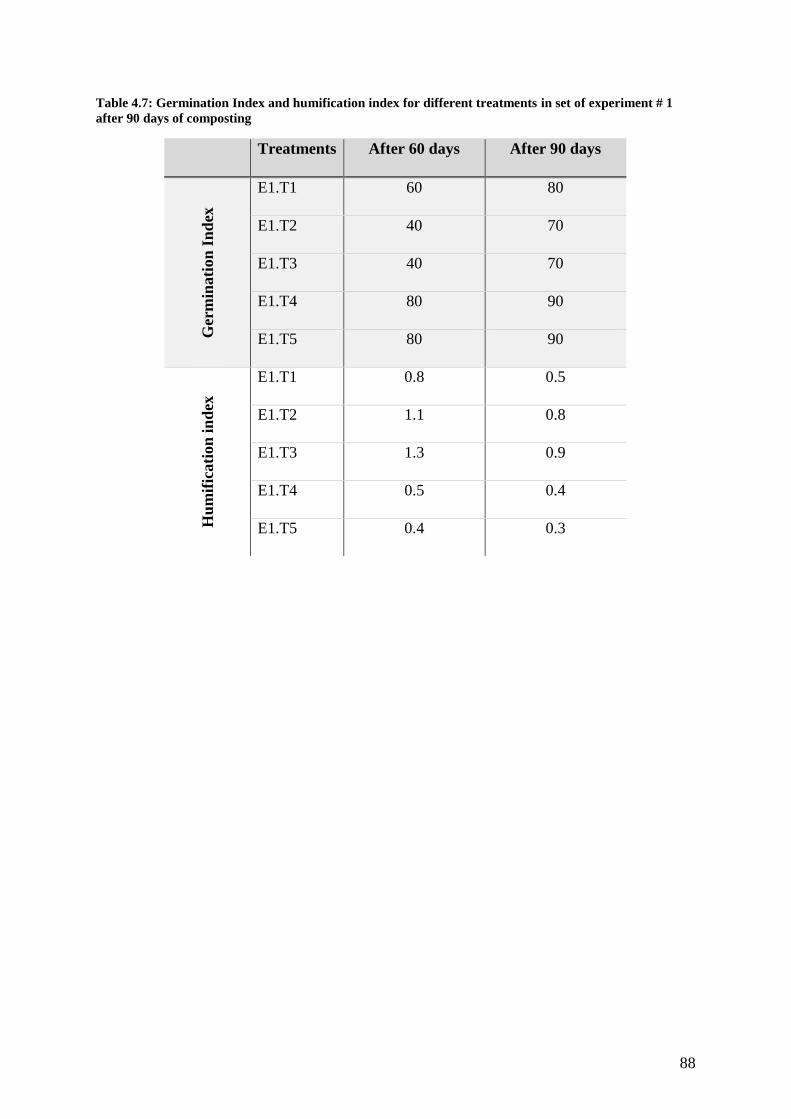
88
Table 4.7: Germination Index and humification index for different treatments in set of experiment # 1
after 90 days of composting
Treatments After 60 days After 90 days
Ger
min
ati
on
In
dex
E1.T1 60 80
E1.T2 40 70
E1.T3 40 70
E1.T4 80 90
E1.T5 80 90
Hu
mif
icati
on
in
dex
E1.T1 0.8 0.5
E1.T2 1.1 0.8
E1.T3 1.3 0.9
E1.T4 0.5 0.4
E1.T5 0.4 0.3
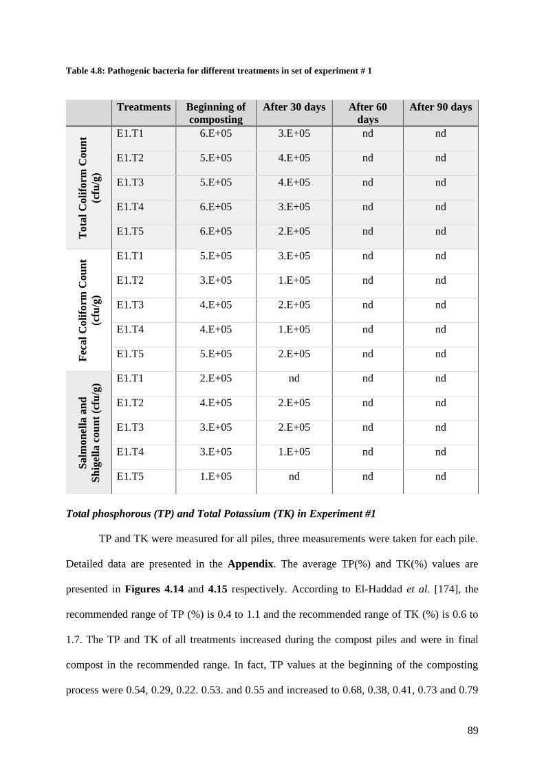
89
Table 4.8: Pathogenic bacteria for different treatments in set of experiment # 1
Total phosphorous (TP) and Total Potassium (TK) in Experiment #1
TP and TK were measured for all piles, three measurements were taken for each pile.
Detailed data are presented in the Appendix. The average TP(%) and TK(%) values are
presented in Figures 4.14 and 4.15 respectively. According to El-Haddad et al. [174], the
recommended range of TP (%) is 0.4 to 1.1 and the recommended range of TK (%) is 0.6 to
1.7. The TP and TK of all treatments increased during the compost piles and were in final
compost in the recommended range. In fact, TP values at the beginning of the composting
process were 0.54, 0.29, 0.22. 0.53. and 0.55 and increased to 0.68, 0.38, 0.41, 0.73 and 0.79
Treatments Beginning of
composting
After 30 days After 60
days
After 90 days
Tota
l C
oli
form
Cou
nt
(cfu
/g)
E1.T1 6.E+05 3.E+05 nd nd
E1.T2 5.E+05 4.E+05 nd nd
E1.T3 5.E+05 4.E+05 nd nd
E1.T4 6.E+05 3.E+05 nd nd
E1.T5 6.E+05 2.E+05 nd nd
Fec
al
Coli
form
Cou
nt
(cfu
/g)
E1.T1 5.E+05 3.E+05 nd nd
E1.T2 3.E+05 1.E+05 nd nd
E1.T3 4.E+05 2.E+05 nd nd
E1.T4 4.E+05 1.E+05 nd nd
E1.T5 5.E+05 2.E+05 nd nd
Salm
on
ella
an
d
Sh
igel
la c
ou
nt
(cfu
/g)
E1.T1 2.E+05 nd nd nd
E1.T2 4.E+05 2.E+05 nd nd
E1.T3 3.E+05 2.E+05 nd nd
E1.T4 3.E+05 1.E+05 nd nd
E1.T5 1.E+05 nd nd nd
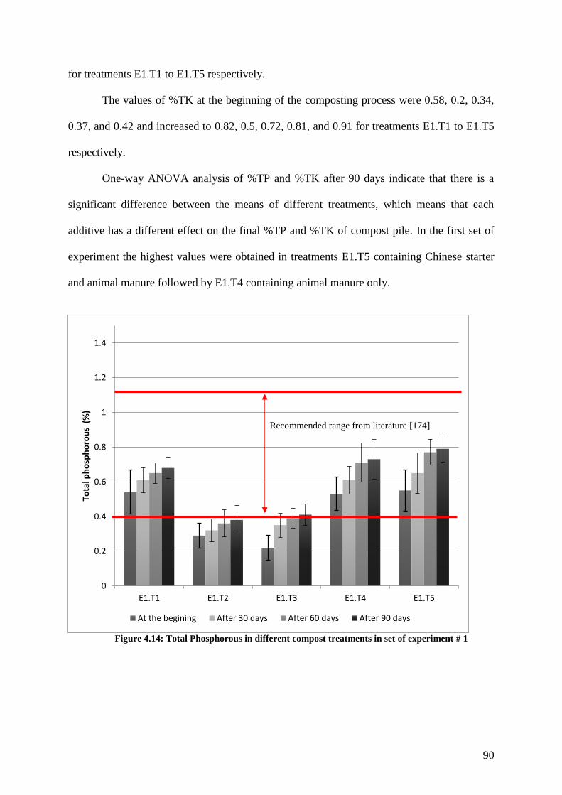
90
for treatments E1.T1 to E1.T5 respectively.
The values of %TK at the beginning of the composting process were 0.58, 0.2, 0.34,
0.37, and 0.42 and increased to 0.82, 0.5, 0.72, 0.81, and 0.91 for treatments E1.T1 to E1.T5
respectively.
One-way ANOVA analysis of %TP and %TK after 90 days indicate that there is a
significant difference between the means of different treatments, which means that each
additive has a different effect on the final %TP and %TK of compost pile. In the first set of
experiment the highest values were obtained in treatments E1.T5 containing Chinese starter
and animal manure followed by E1.T4 containing animal manure only.
Figure 4.14: Total Phosphorous in different compost treatments in set of experiment # 1
0
0.2
0.4
0.6
0.8
1
1.2
1.4
E1.T1 E1.T2 E1.T3 E1.T4 E1.T5
Tota
l ph
osp
ho
rou
s (
%)
At the begining After 30 days After 60 days After 90 days
Recommended range from literature [174]
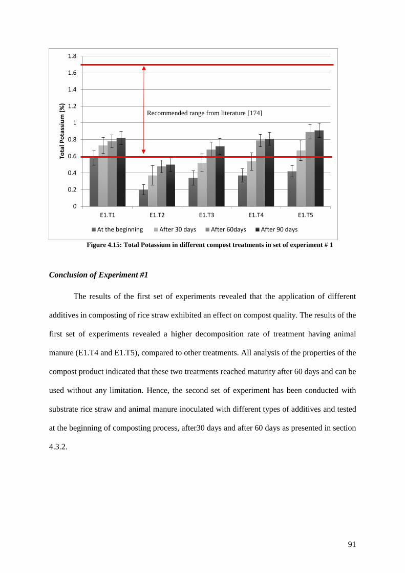
91
Figure 4.15: Total Potassium in different compost treatments in set of experiment # 1
Conclusion of Experiment #1
The results of the first set of experiments revealed that the application of different
additives in composting of rice straw exhibited an effect on compost quality. The results of the
first set of experiments revealed a higher decomposition rate of treatment having animal
manure (E1.T4 and E1.T5), compared to other treatments. All analysis of the properties of the
compost product indicated that these two treatments reached maturity after 60 days and can be
used without any limitation. Hence, the second set of experiment has been conducted with
substrate rice straw and animal manure inoculated with different types of additives and tested
at the beginning of composting process, after30 days and after 60 days as presented in section
4.3.2.
0
0.2
0.4
0.6
0.8
1
1.2
1.4
1.6
1.8
E1.T1 E1.T2 E1.T3 E1.T4 E1.T5
Tota
l Po
tass
ium
(%
)
At the beginning After 30 days After 60days After 90 days
Recommended range from literature [174]
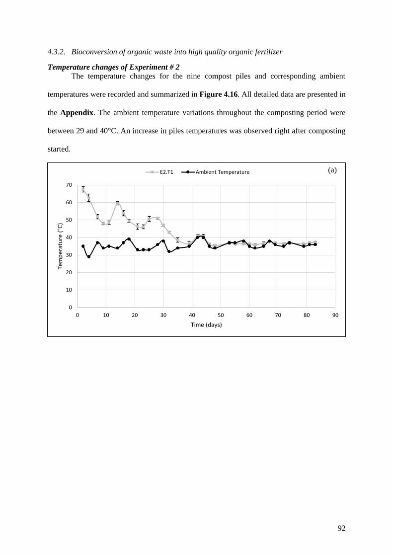
92
4.3.2. Bioconversion of organic waste into high quality organic fertilizer
Temperature changes of Experiment # 2
The temperature changes for the nine compost piles and corresponding ambient
temperatures were recorded and summarized in Figure 4.16. All detailed data are presented in
the Appendix. The ambient temperature variations throughout the composting period were
between 29 and 40°C. An increase in piles temperatures was observed right after composting
started.
0
10
20
30
40
50
60
70
0 10 20 30 40 50 60 70 80 90
Tem
per
atu
re (
°C)
Time (days)
E2.T1 Ambient Temperature (a)
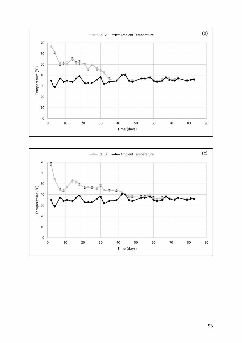
93
0
10
20
30
40
50
60
70
0 10 20 30 40 50 60 70 80 90
Tem
per
atu
re (
°C)
Time (days)
E2.T2 Ambient Temperature
0
10
20
30
40
50
60
70
0 10 20 30 40 50 60 70 80 90
Tem
per
atu
re (
°C)
Time (days)
E2.T3 Ambient Temperature
(b)
(c)
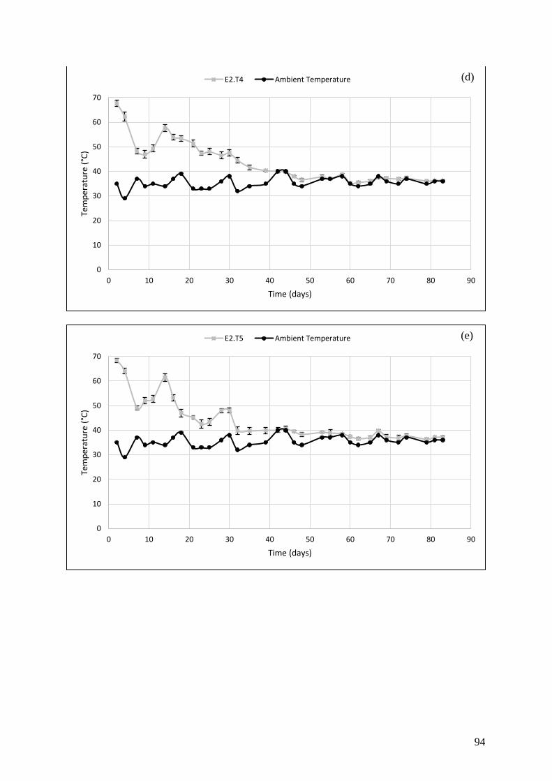
94
0
10
20
30
40
50
60
70
0 10 20 30 40 50 60 70 80 90
Tem
per
atu
re (
°C)
Time (days)
E2.T4 Ambient Temperature
0
10
20
30
40
50
60
70
0 10 20 30 40 50 60 70 80 90
Tem
per
atu
re (
°C)
Time (days)
E2.T5 Ambient Temperature
(d)
(e)
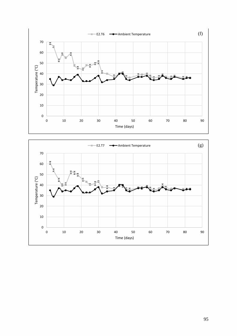
95
0
10
20
30
40
50
60
70
0 10 20 30 40 50 60 70 80 90
Tem
per
atu
re (
°C)
Time (days)
E2.T6 Ambient Temperature
0
10
20
30
40
50
60
70
0 10 20 30 40 50 60 70 80 90
Tem
per
atu
re (
°C)
Time (days)
E2.T7 Ambient Temperature
(f)
(g)
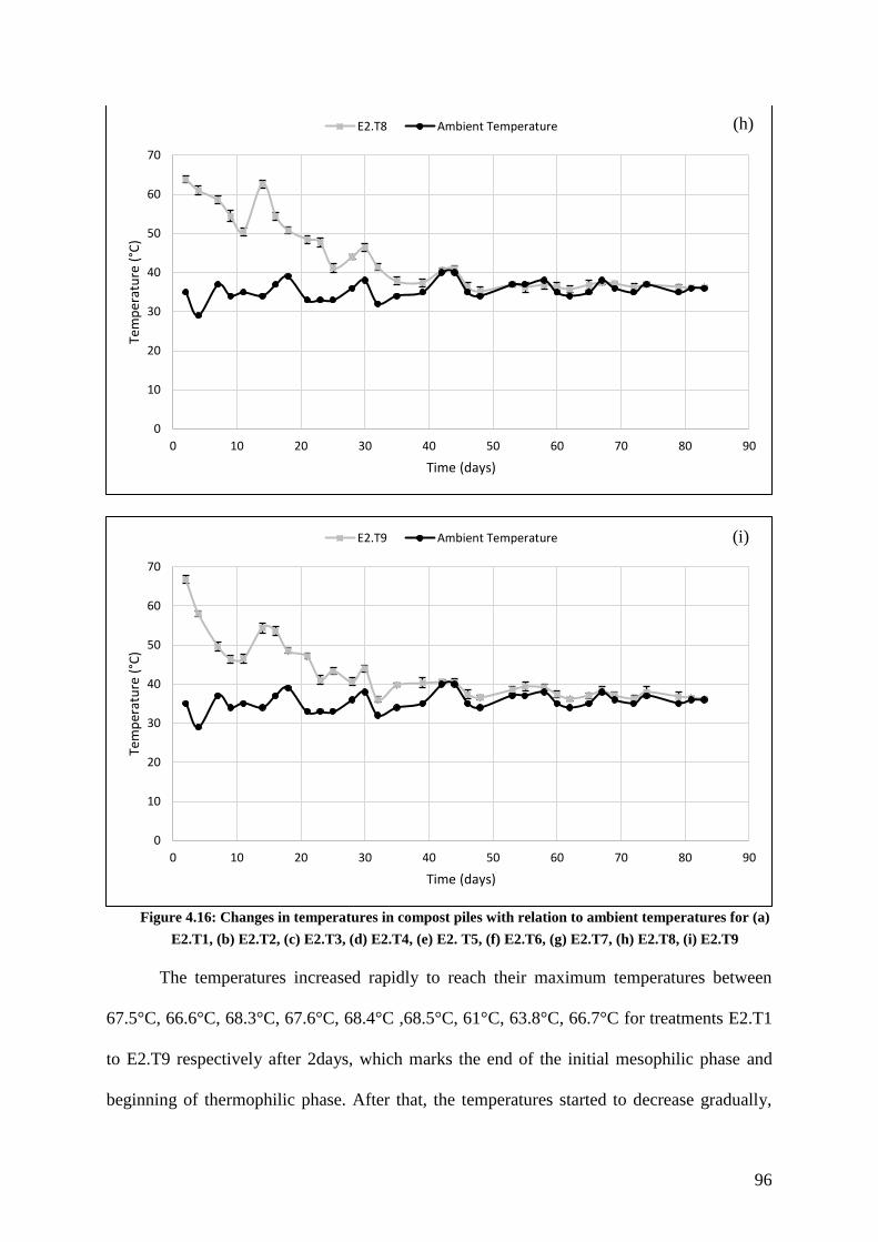
96
Figure 4.16: Changes in temperatures in compost piles with relation to ambient temperatures for (a)
E2.T1, (b) E2.T2, (c) E2.T3, (d) E2.T4, (e) E2. T5, (f) E2.T6, (g) E2.T7, (h) E2.T8, (i) E2.T9
The temperatures increased rapidly to reach their maximum temperatures between
67.5°C, 66.6°C, 68.3°C, 67.6°C, 68.4°C ,68.5°C, 61°C, 63.8°C, 66.7°C for treatments E2.T1
to E2.T9 respectively after 2days, which marks the end of the initial mesophilic phase and
beginning of thermophilic phase. After that, the temperatures started to decrease gradually,
0
10
20
30
40
50
60
70
0 10 20 30 40 50 60 70 80 90
Tem
per
atu
re (
°C)
Time (days)
E2.T8 Ambient Temperature
0
10
20
30
40
50
60
70
0 10 20 30 40 50 60 70 80 90
Tem
per
atu
re (
°C)
Time (days)
E2.T9 Ambient Temperature
(h)
(i)
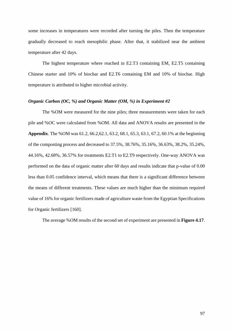
97
some increases in temperatures were recorded after turning the piles. Then the temperature
gradually decreased to reach mesophilic phase. After that, it stabilized near the ambient
temperature after 42 days.
The highest temperature where reached in E2.T3 containing EM, E2.T5 containing
Chinese starter and 10% of biochar and E2.T6 containing EM and 10% of biochar. High
temperature is attributed to higher microbial activity.
Organic Carbon (OC, %) and Organic Matter (OM, %) in Experiment #2
The %OM were measured for the nine piles; three measurements were taken for each
pile and %OC were calculated from %OM. All data and ANOVA results are presented in the
Appendix. The %OM was 61.2, 66.2,62.1, 63.2, 68.1, 65.3, 63.1, 67.2, 60.1% at the beginning
of the composting process and decreased to 37.5%, 38.76%, 35.16%, 36.63%, 38.2%, 35.24%,
44.16%, 42.68%, 36.57% for treatments E2.T1 to E2.T9 respectively. One-way ANOVA was
performed on the data of organic matter after 60 days and results indicate that p-value of 0.00
less than 0.05 confidence interval, which means that there is a significant difference between
the means of different treatments. These values are much higher than the minimum required
value of 16% for organic fertilizers made of agriculture waste from the Egyptian Specifications
for Organic fertilizers [160].
The average %OM results of the second set of experiment are presented in Figure 4.17.
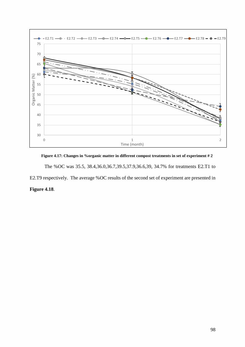
98
Figure 4.17: Changes in %organic matter in different compost treatments in set of experiment # 2
The %OC was 35.5, 38.4,36.0,36.7,39.5,37.9,36.6,39, 34.7% for treatments E2.T1 to
E2.T9 respectively. The average %OC results of the second set of experiment are presented in
Figure 4.18.
30
35
40
45
50
55
60
65
70
75
0 1 2
Org
anic
Mat
ter
(%)
Time (month)
E2.T1 E2.T2 E2.T3 E2.T4 E2.T5 E2.T6 E2.T7 E2.T8 E2.T9
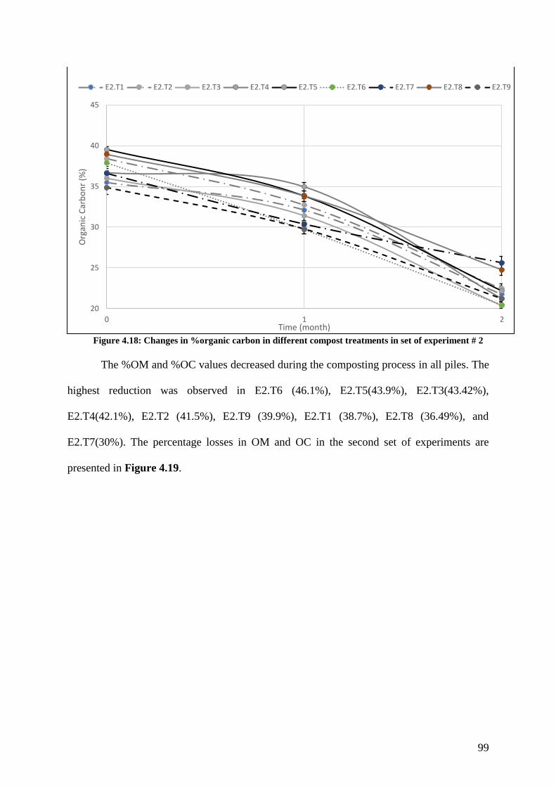
99
Figure 4.18: Changes in %organic carbon in different compost treatments in set of experiment # 2
The %OM and %OC values decreased during the composting process in all piles. The
highest reduction was observed in E2.T6 (46.1%), E2.T5(43.9%), E2.T3(43.42%),
E2.T4(42.1%), E2.T2 (41.5%), E2.T9 (39.9%), E2.T1 (38.7%), E2.T8 (36.49%), and
E2.T7(30%). The percentage losses in OM and OC in the second set of experiments are
presented in Figure 4.19.
20
25
30
35
40
45
0 1 2
Org
anic
Car
bo
nr
(%)
Time (month)
E2.T1 E2.T2 E2.T3 E2.T4 E2.T5 E2.T6 E2.T7 E2.T8 E2.T9
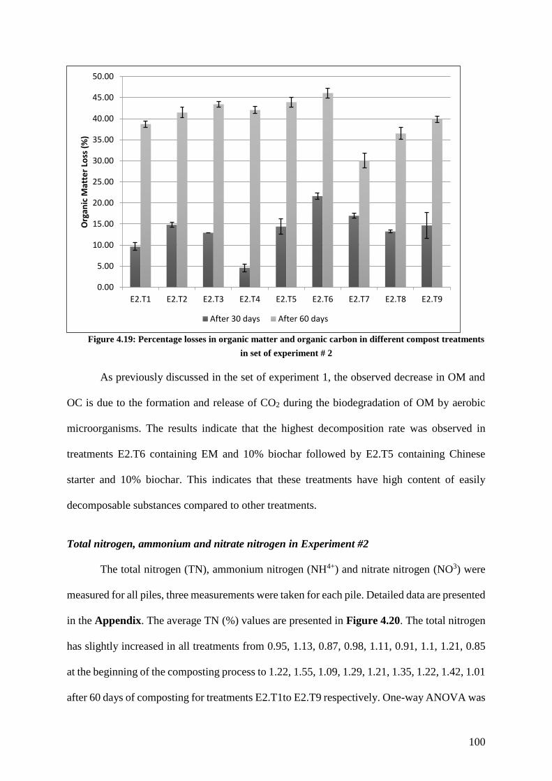
100
Figure 4.19: Percentage losses in organic matter and organic carbon in different compost treatments
in set of experiment # 2
As previously discussed in the set of experiment 1, the observed decrease in OM and
OC is due to the formation and release of CO2 during the biodegradation of OM by aerobic
microorganisms. The results indicate that the highest decomposition rate was observed in
treatments E2.T6 containing EM and 10% biochar followed by E2.T5 containing Chinese
starter and 10% biochar. This indicates that these treatments have high content of easily
decomposable substances compared to other treatments.
Total nitrogen, ammonium and nitrate nitrogen in Experiment #2
The total nitrogen (TN), ammonium nitrogen (NH4+) and nitrate nitrogen (NO3) were
measured for all piles, three measurements were taken for each pile. Detailed data are presented
in the Appendix. The average TN (%) values are presented in Figure 4.20. The total nitrogen
has slightly increased in all treatments from 0.95, 1.13, 0.87, 0.98, 1.11, 0.91, 1.1, 1.21, 0.85
at the beginning of the composting process to 1.22, 1.55, 1.09, 1.29, 1.21, 1.35, 1.22, 1.42, 1.01
after 60 days of composting for treatments E2.T1to E2.T9 respectively. One-way ANOVA was
0.00
5.00
10.00
15.00
20.00
25.00
30.00
35.00
40.00
45.00
50.00
E2.T1 E2.T2 E2.T3 E2.T4 E2.T5 E2.T6 E2.T7 E2.T8 E2.T9
Org
anic
Mat
ter
Loss
(%
)
After 30 days After 60 days
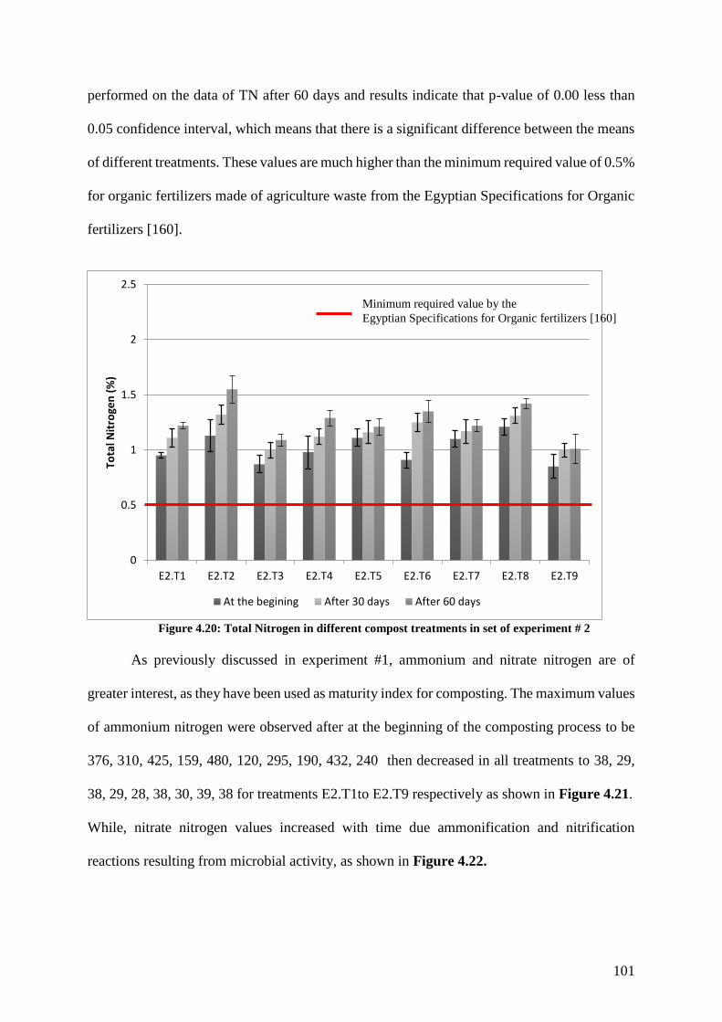
101
performed on the data of TN after 60 days and results indicate that p-value of 0.00 less than
0.05 confidence interval, which means that there is a significant difference between the means
of different treatments. These values are much higher than the minimum required value of 0.5%
for organic fertilizers made of agriculture waste from the Egyptian Specifications for Organic
fertilizers [160].
Figure 4.20: Total Nitrogen in different compost treatments in set of experiment # 2
As previously discussed in experiment #1, ammonium and nitrate nitrogen are of
greater interest, as they have been used as maturity index for composting. The maximum values
of ammonium nitrogen were observed after at the beginning of the composting process to be
376, 310, 425, 159, 480, 120, 295, 190, 432, 240 then decreased in all treatments to 38, 29,
38, 29, 28, 38, 30, 39, 38 for treatments E2.T1to E2.T9 respectively as shown in Figure 4.21.
While, nitrate nitrogen values increased with time due ammonification and nitrification
reactions resulting from microbial activity, as shown in Figure 4.22.
0
0.5
1
1.5
2
2.5
E2.T1 E2.T2 E2.T3 E2.T4 E2.T5 E2.T6 E2.T7 E2.T8 E2.T9
Tota
l Nit
roge
n (
%)
At the begining After 30 days After 60 days
Minimum required value by the
Egyptian Specifications for Organic fertilizers [160]
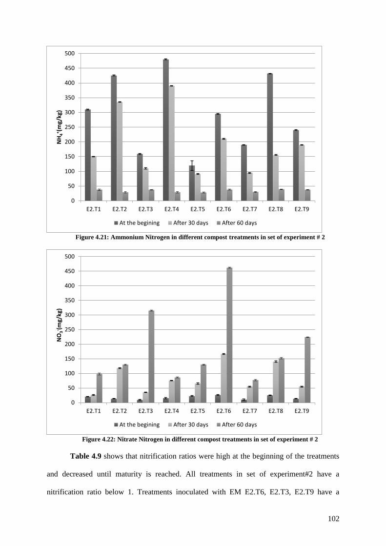
102
Figure 4.21: Ammonium Nitrogen in different compost treatments in set of experiment # 2
Figure 4.22: Nitrate Nitrogen in different compost treatments in set of experiment # 2
Table 4.9 shows that nitrification ratios were high at the beginning of the treatments
and decreased until maturity is reached. All treatments in set of experiment#2 have a
nitrification ratio below 1. Treatments inoculated with EM E2.T6, E2.T3, E2.T9 have a
0
50
100
150
200
250
300
350
400
450
500
E2.T1 E2.T2 E2.T3 E2.T4 E2.T5 E2.T6 E2.T7 E2.T8 E2.T9
NH
4+ (m
g/kg
)
At the begining After 30 days After 60 days
0
50
100
150
200
250
300
350
400
450
500
E2.T1 E2.T2 E2.T3 E2.T4 E2.T5 E2.T6 E2.T7 E2.T8 E2.T9
NO
3- (
mg/
kg)
At the begining After 30 days After 60 days
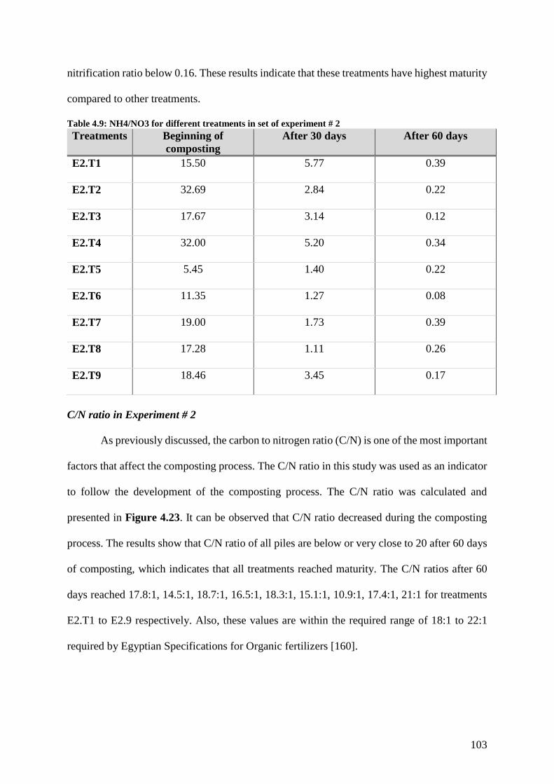
103
nitrification ratio below 0.16. These results indicate that these treatments have highest maturity
compared to other treatments.
Table 4.9: NH4/NO3 for different treatments in set of experiment # 2
Treatments Beginning of
composting
After 30 days After 60 days
E2.T1 15.50 5.77 0.39
E2.T2 32.69 2.84 0.22
E2.T3 17.67 3.14 0.12
E2.T4 32.00 5.20 0.34
E2.T5 5.45 1.40 0.22
E2.T6 11.35 1.27 0.08
E2.T7 19.00 1.73 0.39
E2.T8 17.28 1.11 0.26
E2.T9 18.46 3.45 0.17
C/N ratio in Experiment # 2
As previously discussed, the carbon to nitrogen ratio (C/N) is one of the most important
factors that affect the composting process. The C/N ratio in this study was used as an indicator
to follow the development of the composting process. The C/N ratio was calculated and
presented in Figure 4.23. It can be observed that C/N ratio decreased during the composting
process. The results show that C/N ratio of all piles are below or very close to 20 after 60 days
of composting, which indicates that all treatments reached maturity. The C/N ratios after 60
days reached 17.8:1, 14.5:1, 18.7:1, 16.5:1, 18.3:1, 15.1:1, 10.9:1, 17.4:1, 21:1 for treatments
E2.T1 to E2.9 respectively. Also, these values are within the required range of 18:1 to 22:1
required by Egyptian Specifications for Organic fertilizers [160].
104
Figure 4.23: C/N ratio in different compost treatments in set of experiment # 2
Moisture content and bulk density in Experiment #2
The moisture content and bulk density were measured for all piles as presented in
Figures 4.24 and 4.25 respectively.
The moisture content of all treatments initially ranged from 67-60% and decreased
during the composting process to reach values in the range of 30 to 38%. It is worth mentioning
that treatments E2.T4, E2.T5 and E2.T6 contain 10% biochar compared to other treatments.
This could be because biochar has high water holding capacities as recent studies indicated
[116, 175].
In the first set of experiments, the bulk densities were initially 285 kg/m3, 320 kg/m3,
300 kg/m3, 210 kg/m3 and 290 kg/m3 280 kg/m3, 310 kg/m3, 320 kg/m3, 270 kg/m3 respectively.
These values increased to 445 kg/m3, 533 kg/m3, 470 kg/m3, 420 kg/m3, 536 kg/m3, 480 kg/m3,
494 kg/m3, 552 kg/m3, 466 kg/m3 respectively.
0
10
20
30
40
50
60
70
E2.T1 E2.T2 E2.T3 E2.T4 E2.T5 E2.T6 E2.T7 E2.T8 E2.T9
C/N
rat
io
At the begining After 30 days After 60 days
Range required value by the
Egyptian Specifications for Organic fertilizers [160]
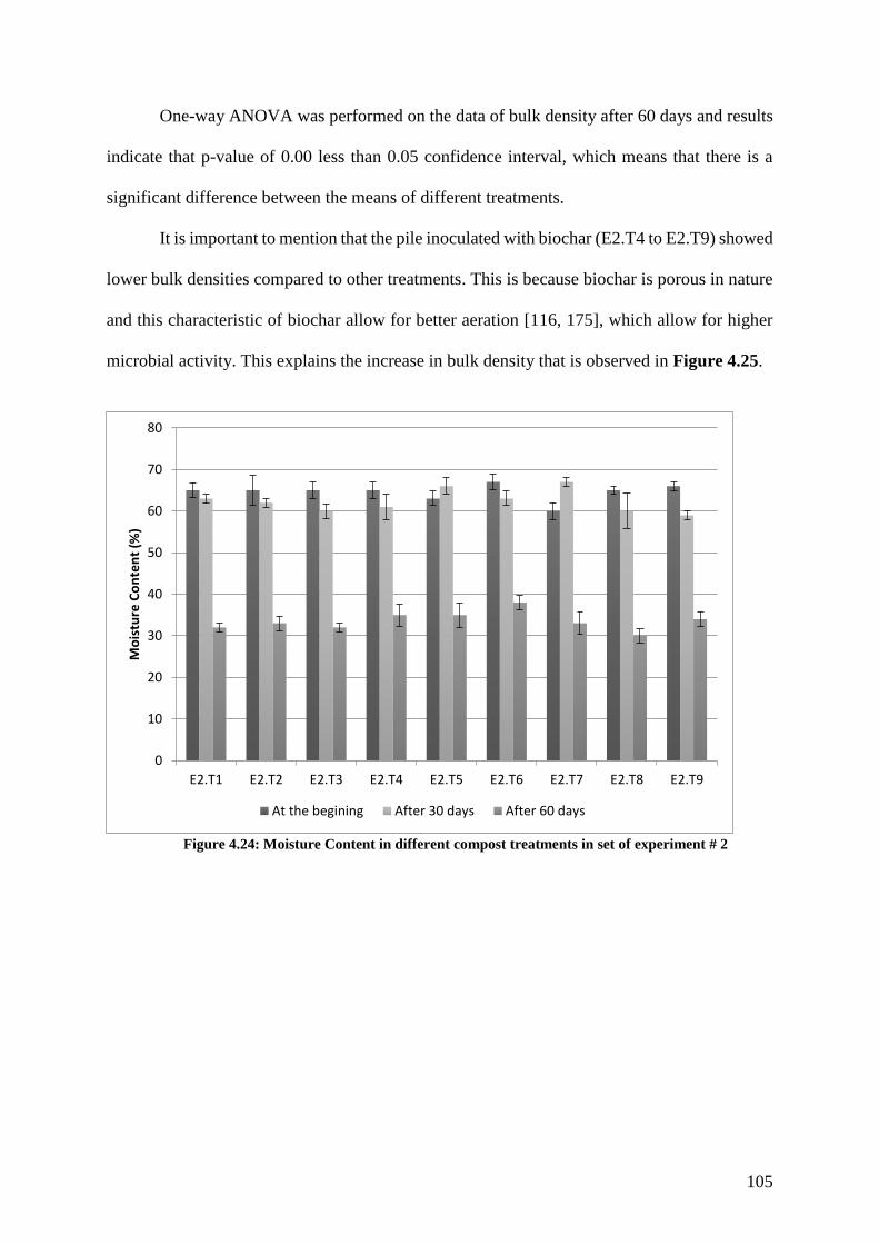
105
One-way ANOVA was performed on the data of bulk density after 60 days and results
indicate that p-value of 0.00 less than 0.05 confidence interval, which means that there is a
significant difference between the means of different treatments.
It is important to mention that the pile inoculated with biochar (E2.T4 to E2.T9) showed
lower bulk densities compared to other treatments. This is because biochar is porous in nature
and this characteristic of biochar allow for better aeration [116, 175], which allow for higher
microbial activity. This explains the increase in bulk density that is observed in Figure 4.25.
Figure 4.24: Moisture Content in different compost treatments in set of experiment # 2
0
10
20
30
40
50
60
70
80
E2.T1 E2.T2 E2.T3 E2.T4 E2.T5 E2.T6 E2.T7 E2.T8 E2.T9
Mo
istu
re C
on
ten
t (%
)
At the begining After 30 days After 60 days
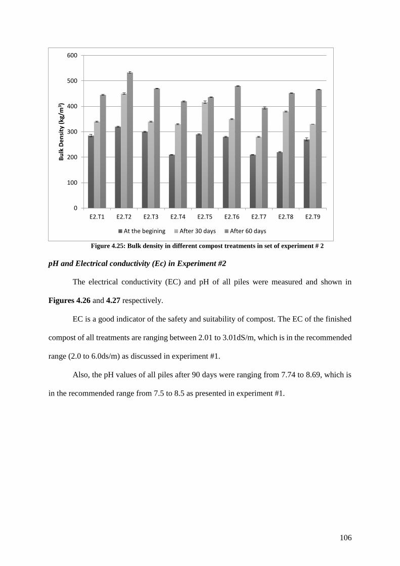
106
Figure 4.25: Bulk density in different compost treatments in set of experiment # 2
pH and Electrical conductivity (Ec) in Experiment #2
The electrical conductivity (EC) and pH of all piles were measured and shown in
Figures 4.26 and 4.27 respectively.
EC is a good indicator of the safety and suitability of compost. The EC of the finished
compost of all treatments are ranging between 2.01 to 3.01dS/m, which is in the recommended
range (2.0 to 6.0ds/m) as discussed in experiment #1.
Also, the pH values of all piles after 90 days were ranging from 7.74 to 8.69, which is
in the recommended range from 7.5 to 8.5 as presented in experiment #1.
0
100
200
300
400
500
600
E2.T1 E2.T2 E2.T3 E2.T4 E2.T5 E2.T6 E2.T7 E2.T8 E2.T9
Bu
lk D
en
sity
(kg
/m3)
At the begining After 30 days After 60 days
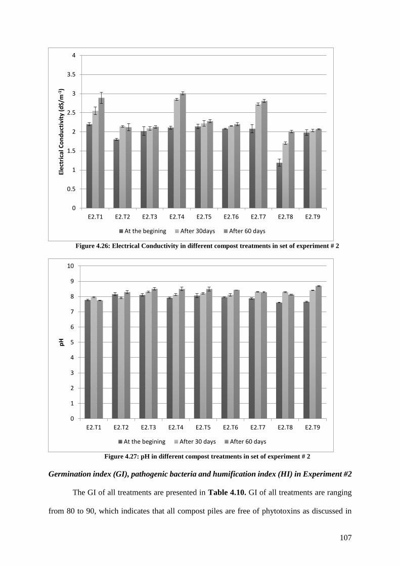
107
Figure 4.26: Electrical Conductivity in different compost treatments in set of experiment # 2
Figure 4.27: pH in different compost treatments in set of experiment # 2
Germination index (GI), pathogenic bacteria and humification index (HI) in Experiment #2
The GI of all treatments are presented in Table 4.10. GI of all treatments are ranging
from 80 to 90, which indicates that all compost piles are free of phytotoxins as discussed in
0
0.5
1
1.5
2
2.5
3
3.5
4
E2.T1 E2.T2 E2.T3 E2.T4 E2.T5 E2.T6 E2.T7 E2.T8 E2.T9
Ele
ctri
cal C
on
du
ctiv
ity
(dS/
m-1
)
At the begining After 30days After 60 days
0
1
2
3
4
5
6
7
8
9
10
E2.T1 E2.T2 E2.T3 E2.T4 E2.T5 E2.T6 E2.T7 E2.T8 E2.T9
pH
At the begining After 30 days After 60 days

108
experiment#1.
The recorded HI are presented in Table 4.10. The recorded HI for all nine treatments
are close to 0.5; therefore, all compost piles could be considered mature.
All final compost treatments were found free of pathogenic bacteria, as presented in Table
4.11, indicating their biosafety.
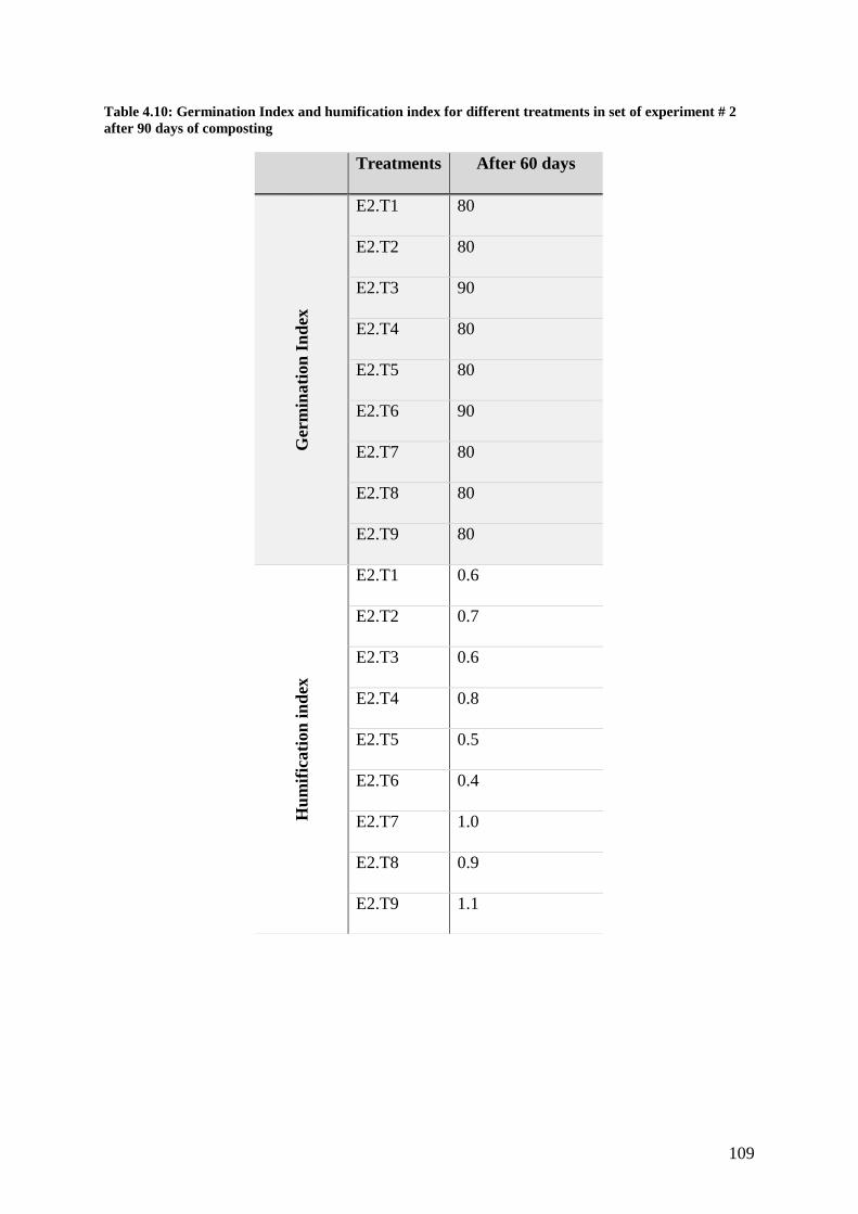
109
Table 4.10: Germination Index and humification index for different treatments in set of experiment # 2
after 90 days of composting
Treatments After 60 days
Ger
min
ati
on
In
dex
E2.T1 80
E2.T2 80
E2.T3 90
E2.T4 80
E2.T5 80
E2.T6 90
E2.T7 80
E2.T8 80
E2.T9 80
Hu
mif
icati
on
in
dex
E2.T1 0.6
E2.T2 0.7
E2.T3 0.6
E2.T4 0.8
E2.T5 0.5
E2.T6 0.4
E2.T7 1.0
E2.T8 0.9
E2.T9 1.1
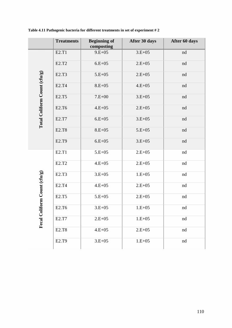
110
Table 4.11 Pathogenic bacteria for different treatments in set of experiment # 2
Treatments Beginning of
composting
After 30 days After 60 days T
ota
l C
oli
form
Cou
nt
(cfu
/g)
E2.T1 9.E+05 3.E+05 nd
E2.T2 6.E+05 2.E+05 nd
E2.T3 5.E+05 2.E+05 nd
E2.T4 8.E+05 4.E+05 nd
E2.T5 7.E+00 3.E+05 nd
E2.T6 4.E+05 2.E+05 nd
E2.T7 6.E+05 3.E+05 nd
E2.T8 8.E+05 5.E+05 nd
E2.T9 6.E+05 3.E+05 nd
Fec
al
Coli
form
Cou
nt
(cfu
/g)
E2.T1 5.E+05 2.E+05 nd
E2.T2 4.E+05 2.E+05 nd
E2.T3 3.E+05 1.E+05 nd
E2.T4 4.E+05 2.E+05 nd
E2.T5 5.E+05 2.E+05 nd
E2.T6 3.E+05 1.E+05 nd
E2.T7 2.E+05 1.E+05 nd
E2.T8 4.E+05 2.E+05 nd
E2.T9 3.E+05 1.E+05 nd
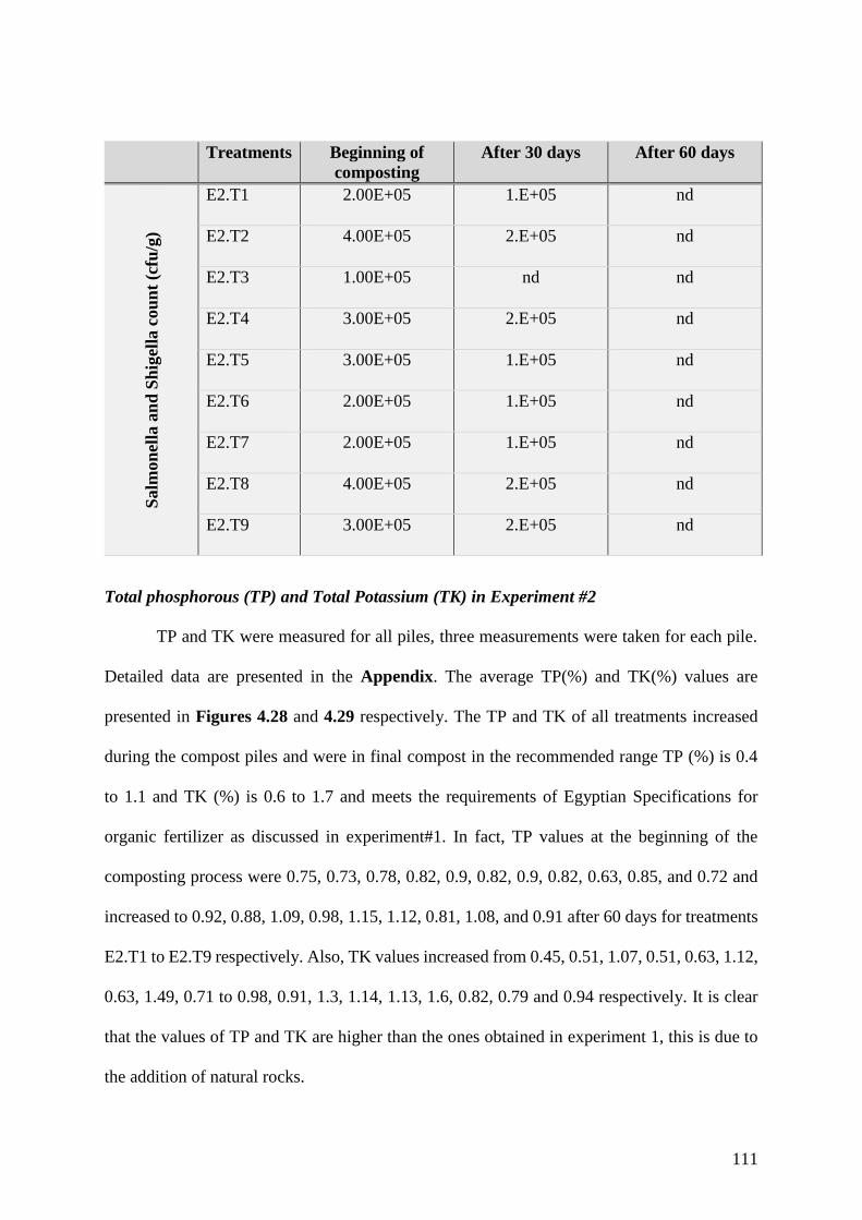
111
Total phosphorous (TP) and Total Potassium (TK) in Experiment #2
TP and TK were measured for all piles, three measurements were taken for each pile.
Detailed data are presented in the Appendix. The average TP(%) and TK(%) values are
presented in Figures 4.28 and 4.29 respectively. The TP and TK of all treatments increased
during the compost piles and were in final compost in the recommended range TP (%) is 0.4
to 1.1 and TK (%) is 0.6 to 1.7 and meets the requirements of Egyptian Specifications for
organic fertilizer as discussed in experiment#1. In fact, TP values at the beginning of the
composting process were 0.75, 0.73, 0.78, 0.82, 0.9, 0.82, 0.9, 0.82, 0.63, 0.85, and 0.72 and
increased to 0.92, 0.88, 1.09, 0.98, 1.15, 1.12, 0.81, 1.08, and 0.91 after 60 days for treatments
E2.T1 to E2.T9 respectively. Also, TK values increased from 0.45, 0.51, 1.07, 0.51, 0.63, 1.12,
0.63, 1.49, 0.71 to 0.98, 0.91, 1.3, 1.14, 1.13, 1.6, 0.82, 0.79 and 0.94 respectively. It is clear
that the values of TP and TK are higher than the ones obtained in experiment 1, this is due to
the addition of natural rocks.
Treatments Beginning of
composting
After 30 days After 60 days S
alm
on
ella
an
d S
hig
ella
cou
nt
(cfu
/g)
E2.T1 2.00E+05 1.E+05 nd
E2.T2 4.00E+05 2.E+05 nd
E2.T3 1.00E+05 nd nd
E2.T4 3.00E+05 2.E+05 nd
E2.T5 3.00E+05 1.E+05 nd
E2.T6 2.00E+05 1.E+05 nd
E2.T7 2.00E+05 1.E+05 nd
E2.T8 4.00E+05 2.E+05 nd
E2.T9 3.00E+05 2.E+05 nd

112
It is important to mention that piles containing 10% of biochar (E2.T4, E2.T5 and
E2.T6) has higher %TP and %TK content. This is attributed to the fact that biochar is rich in
phosphorous and potassium [116, 175].
In the second set of experiment the highest values were obtained in E2.T6 containing
EM and 10% biochar. It is also important to notice that as increasing the percentage of biochar
to 10% has increase quality of the compost. However, further increase of biochar to 20%
decreased the quality of the compost. Similar results are observed by Xiao et al. [116] that
reported that higher rates of biochar may hinder organic matter biodegradation.
Figure 4.28: Total Phosphorous in different compost treatments in set of experiment # 2
0
0.2
0.4
0.6
0.8
1
1.2
1.4
E2.T1 E2.T2 E2.T3 E2.T4 E2.T5 E2.T6 E2.T7 E2.T8 E2.T9
Tota
l ph
osp
ho
rou
s (
%)
At the begining After 30 days After 60 days
Minimum required value by the
Egyptian Specifications for Organic fertilizers [160]
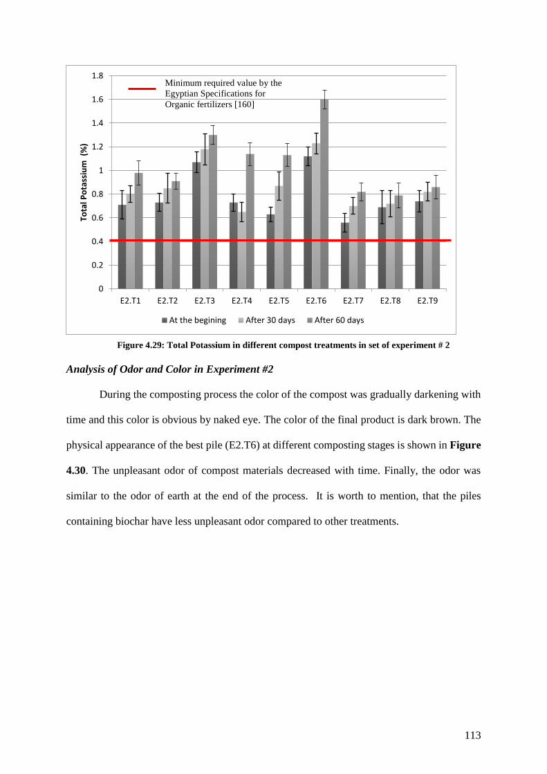
113
Figure 4.29: Total Potassium in different compost treatments in set of experiment # 2
Analysis of Odor and Color in Experiment #2
During the composting process the color of the compost was gradually darkening with
time and this color is obvious by naked eye. The color of the final product is dark brown. The
physical appearance of the best pile (E2.T6) at different composting stages is shown in Figure
4.30. The unpleasant odor of compost materials decreased with time. Finally, the odor was
similar to the odor of earth at the end of the process. It is worth to mention, that the piles
containing biochar have less unpleasant odor compared to other treatments.
0
0.2
0.4
0.6
0.8
1
1.2
1.4
1.6
1.8
E2.T1 E2.T2 E2.T3 E2.T4 E2.T5 E2.T6 E2.T7 E2.T8 E2.T9
Tota
l Po
tass
ium
(%)
At the begining After 30 days After 60 days
Minimum required value by the
Egyptian Specifications for
Organic fertilizers [160]

114
Figure 4.30: Physical appearance of E2.T6 (a) at the beginning of compost process, after (b) 30 days,
(c) 60 days, and (c) 90 days
Conclusion of experiment # 2
In the second set of experiment natural rocks was added to rice straw and animal manure
to enrich the nutritional value and produce high quality organic fertilizer. The effect of different
additives to this substrate was studied and the results revealed that the application of different
additives in composting of rice straw exhibit an improvement in maturation time and final
product quality. In fact, all piles reached maturation after around 42 days. All analysis of the
properties of the final products indicated that it was in the range of the matured level and can
be used without any limitation as an organic fertilizer after 60 days. The highest decomposition
(a) (b)
(c) (d)
115
rate and highest organic fertilizer quality was obtained in pile containing rice straw and 40%
of animal manure mixed with natural rocks (2.5% of rock phosphate, 2.5% feldspar, 2.5%
sulfur, 2.5% dolomite and 10% bentonite) and inoculated with 2% of EM and 10% biochar
compared to other treatments. Also, the results showed that adding 20% biochar decreased the
quality of the final compost compared to adding 10%.
4.4. From organic waste to sustainable green business opportunity in
rural Egypt
Industry Analysis
Challenges facing the fertilizer Industry in Egypt
The tremendous increase in population in Egypt lead to an increase in food and
agricultural production. Thus, many efforts are done to increase agricultural production and
improve crop quality. In order to do that, better agricultural production methods are adopted to
farm various types of yields. One of the most important factors to improve quality of agriculture
production is the quality of the fertilizer used.
In Egypt, chemical fertilizers, also known as inorganic fertilizers, are composed of
chemicals and/or minerals and are widely used as they allow fast and short-term plant growth.
Chemical fertilizers can be divided into three main types:
1. Nitrogen Fertilizer (N): have high percentage of nitrogen and Urea and Ammonium
nitrate are the main types of nitrogen fertilizers utilized in Egypt. There are several
types including:
a. urea (46.5 percent N)
b. ammonium nitrate (33.5 percent N)
c. ammonium sulphate (20.6 percent N)
d. calcium nitrate (15.5 percent N)
2. Phosphate Fertilizers (P): the main constituent is Phosphorus. There are several types
116
including:
a. single superphosphate (15 percent P2O5)
b. concentrated superphosphate (37 percent P2O5)
3. Potassium fertilizers (K) is mainly made of potassium, there are several types including:
a. potassium sulphate (48 to 50 percent K2O)
b. potassium chloride (50 to 60 percent K2O)
In Egypt, mineral fertilizers, especially nitrogen, phosphate and potassium are being
applied to an increasing extent. Table 4.12 summarizes the quantities of chemical fertilizers
produced in Egypt compared to the quantities required by the Egyptian farmers. The main
causes of the increase in consumption of chemical fertilizers including:
The increase in cropped area
The farming of different types of crops at high rates required high rates of fertilizers.
The quantity of suspended material deposited on soil which enrich the nutritional
value of the soil decrease with the construction of the High Aswan Dam.
Table 4.12: Demand and Supply of chemical fertilizer in Egypt [176]
Type of
chemical
fertilizer
Quantity
Produced in
Egypt (Tons)
Quantities
available for
Egyptian
market
Demand Average
Annual
Shortage (ton)
Nitrogen
fertilizer
5,045,300 5,400,000 8,300,000 2,900,000
Phosphate
fertilizer
2,345,700 1,900,000 2,300,000 400,000
Potassium
fertilizer
Not produced in
Egypt
259,000 3,400,000 3,141,000
As indicated in Table 4.12, nitrogen fertilizer is the most widely used type of chemical
fertilizer in Egypt as nitrogen, especially urea. The production of nitrogen fertilizers began in
1951 [176]. The difference between the quantity produced in Egypt and quantity available for
the Egyptian market is imported.
As shown in Table 4.12, Egypt produces nitrogen and phosphate fertilizers. Phosphate
117
fertilizer used to be imported until 1936 the local production of Phosphate started in Egypt.
Large part of the produced phosphate fertilizer is exported as indicated in Table 4.12. No
potassium fertilizers are produced in Egypt due to the lack of resources.
There are eight public sectors companies producing chemical fertilizer in Egypt
including Abou Kir, Delta, and Helwan Al-Masriya. Also, there are five privet sector
companies that sell half of their production to the government at subsidies price via the
Principal Bank for Development & Agricultural Credit (PBDAC) and agricultural
cooperatives.
The table indicates that there is an annual shortage of chemical fertilizer in the Egyptian
market.
Challenges facing the demand side (farmers)
Although chemical fertilizers allow plants to grow fast, it has some disadvantages
including the following [177]:
1. High price
2. Excessive use of chemical fertilizers that may lead to accumulation of heavy metals in
soil and plant system. Also, chemical fertilizers are highly soluble in water. Plants
absorb the fertilizers through the soil, they can enter the food chain. Thus, misuse of
chemical fertilizers may lead to waterway contamination, chemical burn of crops,
increase in air pollution, and acidification and mineral depletion of soil
The high cost and excessive use of chemical fertilizers is burden on the farmers. In fact,
according to CAPMAS Egypt is ranked the second among the countries of the world in terms
of the addition rate of a unit of area, which is estimated at 352kg of nitrogen per hectare [177].
Challenges facing the Supply side (government and producers)
As previously stated, there is a shortage in the amount of chemical fertilizers in Egypt.
The chemical fertilizer crisis recurs every year and has a great impact on the Egyptian economy
as the agricultural sector is one of the most important aspects of the Egyptian economy. Any
118
increase in the price of chemical fertilizers is directly translated into an increase in price of
agricultural commodities, which affects the level of living of Egyptian citizens. Therefore, in
Egypt quota is provided by the state-owned Bank PBDAC to subsidized fertilizer to help poor
farm owners. Yet, this system allows the creation of black market as producers, distributors
and landlords buy the fertilizer at subsidized price and sell it at high price close to international
market to make profits.
According to the CAPMAS report, in 2014 (before floating of the Egyptian pound)
Public sector companies producing chemical fertilizers bear subsidy as the price is fixed to be
700LE/ton , while in companies in free-zones export the product at $230/ton which was
equivalent to 1610LE/ton [177]. A strike in prices of chemical fertilizers occurred in past
couple of years and the market price has reached LE5,200 per ton while subsidized fertilizers
are sold at LE3,200 per ton. This leads to huge losses for the public-sector companies. At the
same time, the price of producing chemical fertilizers is expected to increase as this industry
utilize intensive amount of natural gas and electricity, which price is currently increasing.
Porter’s Five Forces Model
The five forces model that can be used to assess the attractiveness of the industry are
discussed below:
Threat of Substitute
o Chemical fertilizers are the main substitute to organic fertilizer. Farmers may
oppose the idea of using organic fertilizer as they have already developed all
the required skills to efficiently use chemical fertilizer so introducing a new
product that they are not familiar with could threaten them. However, due to the
shortage and rise of the price of chemical fertilizer, organic fertilizer is the
future of agriculture
Threat of new entrant
119
o The capital cost of this business is low so many people can enter the market and
easily compete. However, this product is relatively new to rural Egypt and not
many people have the know-how to optimize the composting process.
Bargaining power of supplier:
o Farmers currently burn most of their agricultural waste. Hence, buying the
waste of famers could be an attractive alternative to farmers. Not taking the
waste for free will ensure that farmers will stop burning their waste and sell it.
o Chemical fertilizers can have harmful effects on soil
o The price of chemical fertilizer is constantly increasing. Also, the shortage in
chemical fertilizers (especially nitrogen) force farmers to buy from black market
at high prices
Bargaining power of buyer:
o Organic fertilizer can be used by any farmer and at any scale
Rivalry among existing firms:
o Relatively new product in upper Egypt
Industry Trends
PEST (political, economic, social and technological) analysis is conducted to give an
understanding of external factors affecting the fertilizer industry. Each factor could have
negative and positive impact on the industry. Hence, it is important to have a detailed analysis
as summarized below.
Political trend:
o The Egyptian government aims to transform one and a half million acres of desert
land into agricultural lands to fulfill the increasing high-quality food demand at an
affordable price. The National Project for Reclamation and Cultivation will increase
120
farmland in Egypt by 20%. Hence, the demand on fertilizers will tremendously
increase.
o The government aim to use organic farming to improve the quality of food and life
of Egyptians and increase the local production to increase exports and create more
job opportunities.
o The government is also looking for solutions to resolve the conflict between
subsidies, industrial production and local consumption needs
o The government of Egypt is aiming to achieve sustainable development that leads
to transformational change and real improvements in people’s lives. Therefore, the
government is supporting any ideas to reduce pollution of water, soil and air caused
by extensive utilization of chemical fertilizers.
o Also, the government is tending to make energy savings, particularly in intensive
industries like fertilizers.
o The government is aiming to increase the amount of organic farming to be able to
export more agricultural products.
Economic Trend
o The government favors fertilizer industry as it facilitates the agricultural sector,
which has direct impact on price of products utilized by citizens.
o Increase in demand for jobs opportunities
o Increase in demand of fertilizer to meet the demand for the Mega national
agricultural projects
Social Trend
o The extensive use of chemical fertilizers causes many environmental problems
including water, soil and air pollution. These issues can cause many health
problems.
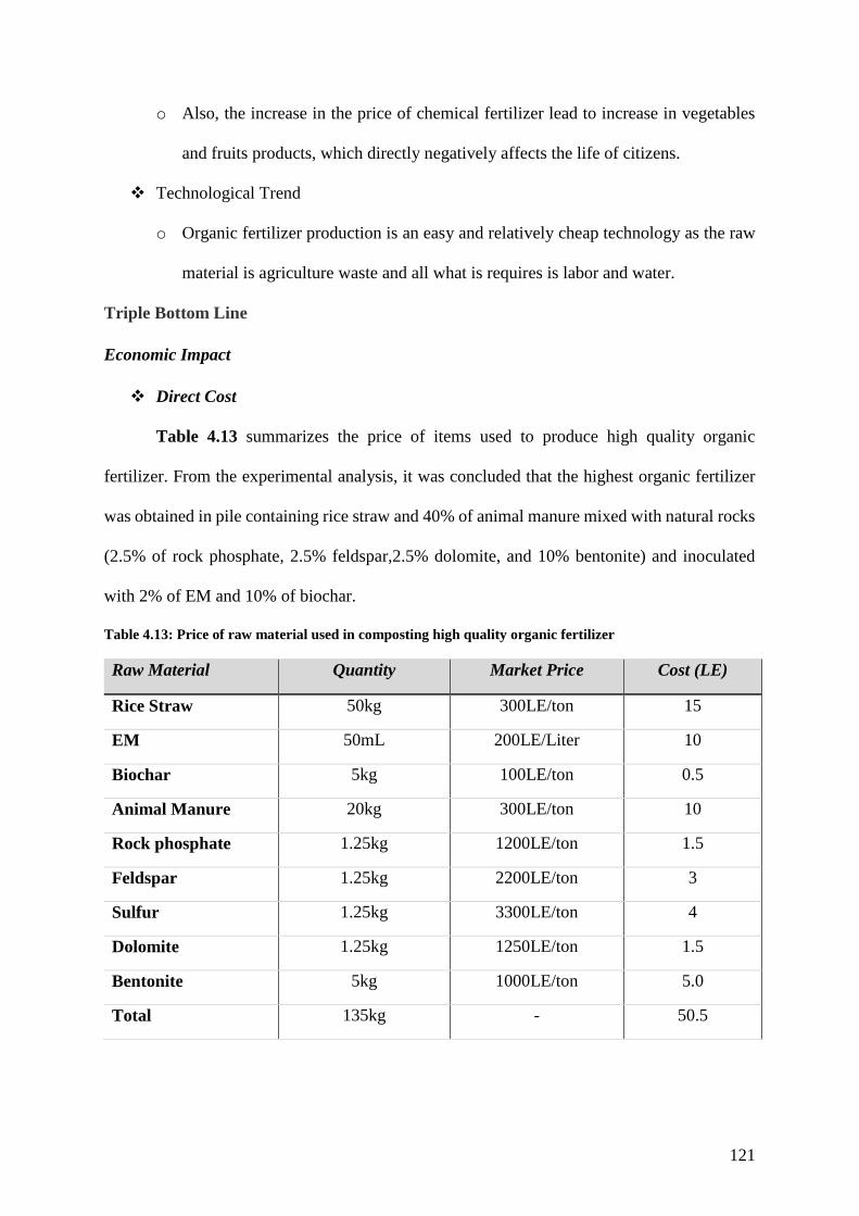
121
o Also, the increase in the price of chemical fertilizer lead to increase in vegetables
and fruits products, which directly negatively affects the life of citizens.
Technological Trend
o Organic fertilizer production is an easy and relatively cheap technology as the raw
material is agriculture waste and all what is requires is labor and water.
Triple Bottom Line
Economic Impact
Direct Cost
Table 4.13 summarizes the price of items used to produce high quality organic
fertilizer. From the experimental analysis, it was concluded that the highest organic fertilizer
was obtained in pile containing rice straw and 40% of animal manure mixed with natural rocks
(2.5% of rock phosphate, 2.5% feldspar,2.5% dolomite, and 10% bentonite) and inoculated
with 2% of EM and 10% of biochar.
Table 4.13: Price of raw material used in composting high quality organic fertilizer
Raw Material Quantity Market Price Cost (LE)
Rice Straw 50kg 300LE/ton 15
EM 50mL 200LE/Liter 10
Biochar 5kg 100LE/ton 0.5
Animal Manure 20kg 300LE/ton 10
Rock phosphate 1.25kg 1200LE/ton 1.5
Feldspar 1.25kg 2200LE/ton 3
Sulfur 1.25kg 3300LE/ton 4
Dolomite 1.25kg 1250LE/ton 1.5
Bentonite 5kg 1000LE/ton 5.0
Total 135kg - 50.5

122
Experiment has shown that there is around 40% loss in weight by the end of the compost
pile. In other words, the initial weight of the pile is 135kg and it produced around 80kg of
organic fertilizer. Hence, the total price is 635LE/ton of organic fertilizer. The price of labor
and transportation was not added as farmers will be turning their compost piles manually in
their lands so no extra charges for labor would be added. Also, this cost could be further
decreased to be 330LE/ton if the farmer will be using the rice straw and animal manure produce
from his land instead of burning it.
Studies conducted on Valencia Orange Trees in Egypt have indicated that on average
using organic fertilizer in combination with other raw materials to increase its nutritional values
would result in similar yield compared to using 100% chemical fertilizer [178, 179, 180].
However, Pradeepkumar et al. [181] conducted a study on ten tropical vegetable crops viz.
amaranthus (Amaranthus tricolor L.), brinjal (Solanum melongena L.), chilli (Capsicum
annuum L.), okra (Abelmoschus esculentus (L.) Moench), tomato (Solanum lycopersicon L.),
bitter gourd (Momordica charantia L.), coleus (Solenostemon rotundifolius (L.) Codd.),
cowpea (Vigna unguiculata (L.) Walp), snake gourd (Trichosanthes anguina L.), and cucumber
(Cucumis sativus L.). This study showed that yields from the use of organic fertilizer is on
average 98% of that obtained from the use of inorganic fertilizer.
Another study conducted by Seekem [182] showed that yields from cotton was 23%
lower than those obtained from chemical fertilizer, yields from peppermint was 29% lower
than the one obtained from chemical fertilizer, while no difference in yield production of dates
was observed.
By using this information, this means the price of 1 ton of the produced organic
fertilizer can be compared to the price of 1 ton of chemical fertilizer. Table 4.14 compares the
prices of produced organic fertilizer with market price of different fertilizers. The presented
123
market price of chemical fertilizer are non-subsidized prices, nitrogen chemical fertilizers are
subsidized and their price is around 40% less than market price.
According to CAPMAS is estimated that in Egypt 352kg of nitrogen chemical fertilizer
is used per hectare [177], which is equivalent to 150kg per feddan. This means that 1 feddan
will require 150kg of organic fertilizer. In other words, urea will cost 810LE/feddan (non-
subsidized price) or 480LE/feddan (subsidized price), while organic fertilizer will cost
95LE/feddan or 50LE/feddan (if the farmer will be using his organic waste to produce the
fertilizer). If the farmer will need labor to produce the fertilizer, according to Mohamed et al.
[178], 1 feddan requires 2 labor for 120LE/feddan each. Therefore, the cost of organic fertilizer
will be cost 335LE/feddan or 290LE/feddan. In other words, the use of organic fertilizer could
be an attractive solution to farmers to substitute the expensive chemical fertilizer and at the
same time could help the government remove the subsidy on chemical fertilizer.

124
Table 4.14: Comparison of price of organic and chemical fertilizer
Type of fertilizer unit Price (LE/ton) Price (LE/feddan)
Organic Fertilizer
Price of organic waste
included labor not included
LE/ton 635 95
Price of organic waste and
labor not included
LE/ton 330 50
Price of organic waste &
labor included
LE/feddan -- 335
Price of organic waste not
included & price of labor
included
LE/feddan -- 290
Chemical Fertilizer Market Price (non-subsidized)
Urea LE/ton 5,400 810
Ammonium nitrate LE/ton 5,600 840
Ammonium Sulphate LE/ton 3,900 585
Calcium nitrate LE/ton 6,000 900
Single superphosphate LE/ton 1,700 255
Concentrated superphosphate LE/ton 1,700 255
Potassium sulphate LE/ton
12,000 1,800
Compound (19N, 19P, 10K) LE/ton
8,400 1,260
Compound (6N,42P, 6K) LE/ton
8,400 1,260
Damage Cost
In addition to the direct cost presented above, there is a hidden external cost that also
must be considered that it will be referred to in this study as “Damage cost”. The data presented
is based on FAO report entitled Food wastage footprint Full-cost accounting – final report”
[183] and Seekem report entitled Future of agriculture in Egypt [184]. There are two main
types of damage cost as follows and their cost is listed in table 4.15:
125
1. Atmosphere damage cost via Greenhouse Gases Emission (GHG)
Several studies were conducted and showed that by applying compost to soil, carbon is
stored in soil. This is due to the fact that composting partly results in the increased formation
of stable carbon compounds, i.e. humus-like substances and aggregates. These are made of
complex compounds that render them resistant to microbial attack. Thus, organic farming is
used as carbon sequestration and GHG emission in organic farming is calculated to be zero.
Carbon sequestration is defined as long-term storage for carbon dioxide. According to FAO
report [183], the damage cost of GHG emission including deforestation and managed organic
soils in the conventional farming is estimated to be $113 per ton CO2 equivalent. These costs
are determined by considering the six most important greenhouse gases: carbon dioxide (CO2),
nitrous oxide (N2O), methane (CH4), hydrofluorocarbons (HFCs), perfluorocarbons (PFCs)
and Sulphur hexafluoride (SF6). These are converted into CO2 equivalents based on their global
warming potential. The atmosphere damage cost is the cost of removing the main GHG from
the atmosphere.
2. Water damage cost
According to Seekem report, water quality cost is determined based on the effect of use
of fertilizer and pesticides in conventional and organic farming. This cost is estimated based
on the cost of removing pesticide, nitrate and phosphate from drinking water. The table below
summarizes the estimated cost for different type of crops. Conventional systems rely on
pesticides many of which are toxic to humans and animals. For organic farming the cost of
pesticides is assumed to be zero.
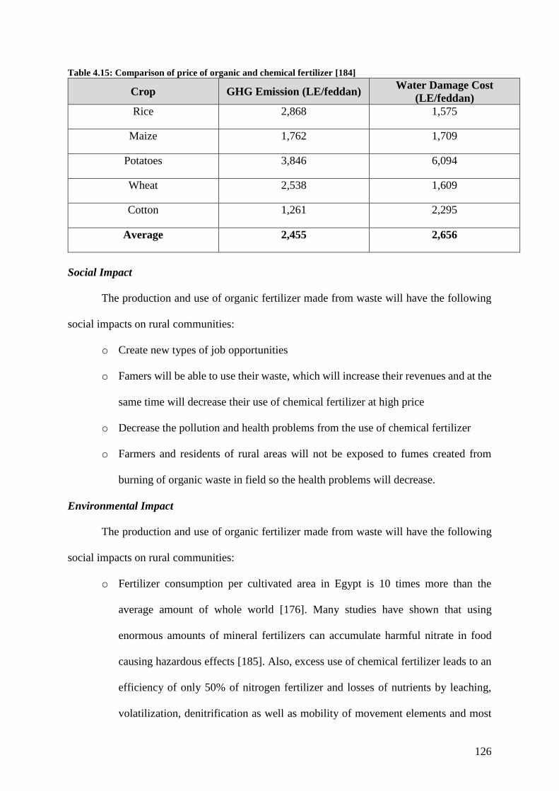
126
Table 4.15: Comparison of price of organic and chemical fertilizer [184]
Crop GHG Emission (LE/feddan) Water Damage Cost
(LE/feddan)
Rice 2,868 1,575
Maize 1,762 1,709
Potatoes 3,846 6,094
Wheat 2,538 1,609
Cotton 1,261 2,295
Average 2,455 2,656
Social Impact
The production and use of organic fertilizer made from waste will have the following
social impacts on rural communities:
o Create new types of job opportunities
o Famers will be able to use their waste, which will increase their revenues and at the
same time will decrease their use of chemical fertilizer at high price
o Decrease the pollution and health problems from the use of chemical fertilizer
o Farmers and residents of rural areas will not be exposed to fumes created from
burning of organic waste in field so the health problems will decrease.
Environmental Impact
The production and use of organic fertilizer made from waste will have the following
social impacts on rural communities:
o Fertilizer consumption per cultivated area in Egypt is 10 times more than the
average amount of whole world [176]. Many studies have shown that using
enormous amounts of mineral fertilizers can accumulate harmful nitrate in food
causing hazardous effects [185]. Also, excess use of chemical fertilizer leads to an
efficiency of only 50% of nitrogen fertilizer and losses of nutrients by leaching,
volatilization, denitrification as well as mobility of movement elements and most
127
of phosphorous and potassium remain inert and only less than 10% of soil content
[186]. Therefore, the use of organic fertilizer will result into a decrease in the
pollution caused from the use of chemical fertilizer
o Decrease the pollution and health problems caused by burning the organic waste
o On the long term the use of organic fertilizer will enrich and rebuild the soil
structure [179, 186].
Key Success Factors
Below is a list of the key elements that should be considered for successful business:
1. Time of Collection from farmers: Waste must be collected from the fields between the
harvest and the planting of the new crop. In fact, farmers burn the waste in the field between
harvest and planting seasons because of lack of storage space. Hence, any delay in
collection could make famers not cooperate.
2. Marketing and education: it is important to educate and market about the benefits of
organic fertilizer compared to chemical fertilizers. It is also important to explain to people
what it is and how it is to be used.
3. Time to apply organic fertilizer: Organic fertilizer should be applied to the soil after the
fermentation process is completed. The addition of organic fertilizer prior to completion of
fermentation process could affect the seed and burn the roots and damage plantation
process. It is imperative to make sure that the organic fertilizer used is stable and mature
before using it, as if fermentation is incomplete the organic fertilizer will burn the soil and
thus farmers will go be to the use of chemical fertilizer.
4. Storage facility: A storage facility is needed to store the collected waste as compost is
seasonal product.
128
5. Diverse type of raw material: The type of waste used should be from different sources
(food waste, different type of crops, etc.) so that the business is not dependent on the
seasonality of the waste and ensure yearlong supply.
6. Gradual shifting of use of organic fertilizer: The shift from chemical to organic fertilizer
must be done gradually.
4.5. Conclusion
The results of the first set of experiments revealed that the application of different
additives in composting of rice straw exhibited an improvement of compost quality. In fact, all
piles reached maturation time after around 60 days. All analysis of the properties of the final
compost products indicated that it was in the range of the matured level and can be used without
any limitation. Yet, the results of the first set of experiments revealed a higher decomposition
rate of treatment having animal manure, compared to other treatments.
Therefore, a second set of experiment has been conducted with substrate rice straw and animal
manure inoculated with different types of additives and mixture of natural rocks to produce
organic fertilizer. The results revealed that the application of different additives in composting
of rice straw exhibit an improvement in maturation time and final product quality. In fact, all
piles reached maturation after around 42 days. All analysis of the properties of the final
products indicated that it was in the range of the matured level and can be used without any
limitation as an organic fertilizer. The highest decomposition rate and highest organic fertilizer
quality was obtained in pile containing rice straw and 40% of animal manure mixed with
natural rocks (2.5% of rock phosphate, 2.5% feldspar, 2.5% sulfur, 2.5% dolomite and 10%
bentonite) and inoculated with 2% of EM and 10% biochar compared to other treatments. Also,
the results showed that adding 20% biochar decreased the quality of the final compost
compared to adding 10%.
129
Applying the Waste to Business (W2B) model introduced in chapter 3 to organic waste in rural
communities indicated that the price of the produced high-quality organic fertilizer is
330LE/ton, given that each farmer will use the organic waste generated from his land and will
not need extra labor to produce the organic fertilizer compared to chemical fertilizer market
price of 1,700LE/ton to 12,000LE/ton (non-subsidized price). In addition to the direct cost, the
use of chemical fertilizer damages the atmosphere and the water. This damage has an
unforeseen high cost. Therefore, organic fertilizer produced from organic waste can substitute
expensive chemical fertilizer. In addition to economic benefits, reducing the use of chemical
fertilizer will lead to the creation of new job opportunities in rural villages, reduction of soil,
water and air pollution as farmers will sell their waste instead of burning it in the field. Also,
application of organic fertilizer will re-establish the soil structure on the long run.
130
CHAPTER 5– APPROACHING FULL UTILIZATION OF
MUNICIPAL SOLID WASTE – CASE STUDY OF REJECTS
5.1. Introduction
One of the major problems facing rural communities in Egypt is poor municipal solid
waste (MSW) management, which contribute to the health, ecological and environmental
problems facing rural communities. According to the country report on the solid waste
management in Egypt in 2014 [11], Egypt generates 21million tons of MSW per year. Most of
municipal solid wastes generated are either burnt or end up in open, public and random
dumpsite or water canals, which contribute to the health, ecological and environmental
problems facing rural communities [5, 6, 22]. More than 35% of waste generated every year in
Egypt is thrown in streets, open dump sites and or water ways causing serious environmental
and health problems [11]. A large amount of waste generated in Egypt is made out of
unrecyclable waste known as rejects [5]. There are many types of rejects and this research
focuses on the following types of rejects: (1) packaging materials, (2) thermosets, and (3)
contaminated plastic bags.
Packaging material could be made of paper and cardboard, glass, aluminum, plastics or
laminated packaging material. The laminated packaging material also known as multilayer
packaging material are usually the ones referred to as rejects as they are hard to recycle because
they are made of multilayer films of different materials bonded together. Multilayer packaging
materials are commonly used to combine different performances of various materials. Hence,
multilayer packaging is created to sufficiently protect sensitive food products and thus obtain
extended shelf life. Usually multi-layer packaging materials are made of three-layers. The inner
side facing the product provides sealability and is usually made of aluminum. The outer layer
provides abrasion resistance, heat resistance, stiffness moisture and oxygen barrier and surface
for printing and is usually made of polyester (PET), polypropylene (PP) and polyethylene (PE).

131
In the center an adhesive is needed to attach two dissimilar materials. Although multilayer
packaging material provide high properties, they usually turn into waste immediately after
using a product and most of them are usually incinerated or landfilled. Large amounts of
packaging materials are generated every year. The Central Department of Solid Waste estimate
that around 29% of MSW in Egypt could be made of packaging materials, which represents 6
million tons [11]. This is not a problem only in developing countries like Egypt, in fact, a study
estimated that 1.89million tons of multi-layer packaging material are generated in Germany in
2009 and it is estimated that 40% of plastic produced in Germany in 2015 is used for packaging
material [187]. It is reported that new law will enter into force in 2019 in Germany to increase
recycling of packaging waste from 40% to 63% by 2022 [187, 188]. Therefore, innovative
solutions to recycle packaging material is required. Most of literature describe recycling of
multilayer packaging material via delamination process to recover either the plastic part and/or
the aluminum side [145, 146, 143, 147, 148]. Some industries in developed countries use
plasma process (around 15000C) to recover aluminum from packaging material [145]. Other
industries use microwave induces pyrolysis, which separates aluminum from plastic laminates
by heating it to a temperature of 500°C [146]. However, because of the high cost and energy
consumption of these techniques, they are not implemented in developing countries. Very few
publications in the literature report mechanical recycling methods to recycle multi-layer
packaging material to produce useful goods [151]. Thus, research is still needed in this area.
Another type of rejects is thermoset, which is a type of plastic that have many attractive
properties (high hardness, thermal resistance, insulation, etc.) making it significantly used in
many applications. All of these properties are attributed to the complex three-dimensional
structure of the material. Yet, this cross-linked nature makes thermosets very challenging to
recycle as they decompose and degrade when subject to heat. Therefore, most of the thermoset
products end up in landfills or are incinerated at the end of their life, which causes serious
132
environmental concerns due to the fact that plastic waste contains various toxic elements,
which can pollute soil and water [23, 24]. Due to the increasing environmental concern,
recycling of non-biodegradable thermoset wastes has been the major issue for researchers [25].
Therefore, the aim of this research is to develop easy and cheap technology to recycle rejects
to produce useful goods. This part of the research will focus on recycling of melamine-
formaldehyde (a hard thermoset), ethylene-propylene-diene- monomer rubber (an elastic
thermoset) and multi-layer flexible packaging material to produce useful goods including
interlock paving units and bricks.
5.2. Objectives
The main aim of this part is to propose solution to economically close the loop for
rejects from municipal solid waste and approach full utilization of rejects. In this part of the
research two innovative, efficient, simple and cheap technologies/products are proposed to
recycle rejects:
Hot Technology
The objectives of this section are to:
Produce an innovative composite material from rejects using compression molding
technique. The composite material is made of multi-layer packaging material as the
matrix and melamine-formaldehyde (one type of hard thermoset) as filling material.
Measure the following mechanical properties of the new composite material:
o Compressive strength in accordance with ASTM D 695 – “Standard Test
Method for Compressive Properties of Rigid Plastics”
o Density
o Water Absorption in accordance with ASTM D 570 – “Standard Test Method
for Water Absorption of Plastics”
o Abrasion Resistance
133
o Abrasion Index
o Flexural strength in accordance with ASTM D 790 – “Standard Test Method
for Flexural Properties of Unreinforced and Reinforced Plastics and Electrical
Insulating Materials”
o Leachate
Conduct full design of experiment using Design Expert 11 software to:
o Identify the effect of three parameters of compression molding (temperature,
percentage filling material, grain size of melamine-formaldehyde) on the
properties of the produced composite material
o Identify the parameter that has the most significant effect on material properties
o Develop equations that will allow the prediction of properties for any
combination of parameters
Compare the measured properties with ASTM Specification requirements for interlock
paving units
Compare mechanical properties obtained if filling material (melamine-formaldehyde)
is substituted with rubber or sand
Compare mechanical properties obtained if packaging material is substituted with
plastic bags
Compare the cost of produced interlock from rejects and commercially available
interlock paving unit
Cold Technology
The objectives of this section are to:
Develop an innovative technique to produce bricks from waste rejects with minimal
energy cost
Measure the following mechanical properties:
134
o Compressive strength in accordance with ASTM C140
o Water Absorption in accordance with ASTM C140
Compare the measure properties with ASTM C129 and the Egyptian code for non-load
bearing masonry bricks
Compare the cost of produced brick from rejects and commercially available brick
5.3. Development of an innovative composite material to produce interlock
paving units from rejects using hot technology
5.3.1. Methodology
Material
Five types of waste rejects are used in these experiments:
Multi-layer Packaging Material (MP) – MP are collected from Hay el Zabaleen in Cairo
from municipal solid waste. These MP are mainly remaining from chips and chocolate
packs, etc. They are mainly composed of three layers aluminum foil, adhesive and
polymeric film usually made of polyethylene, polypropylene, polyamide, etc.
Melamine-formaldehyde (MF) – Old plates made of MF are collected, cleaned and
crushed into powder
EPDM rubber – waste EPDM rubber in form of powder is received from the waste of
ElShark Factory for Rubber – Dorgham.
Sand
Waste contaminated plastic bags
Experimental Procedure
Experiment 1 – Multi-layer Packaging material (MP)+ melamine-formaldehyde
(MF)
MP is shredded into small pieces using a shredding machine as shown in Figure 5.1. MF was
shredded and screened using wire mesh to the following particle sizes:
Sieve 16 (1.18mm)
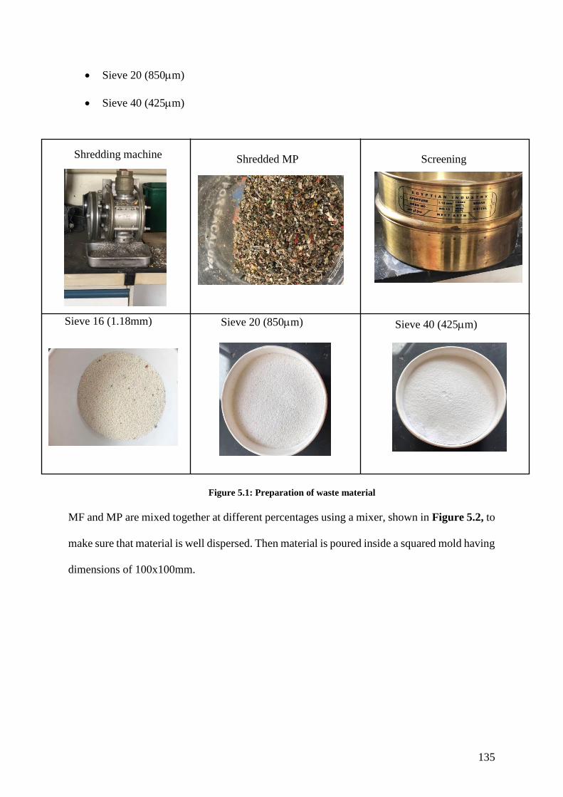
135
Sieve 20 (850m)
Sieve 40 (425m)
Figure 5.1: Preparation of waste material
MF and MP are mixed together at different percentages using a mixer, shown in Figure 5.2, to
make sure that material is well dispersed. Then material is poured inside a squared mold having
dimensions of 100x100mm.
Shredding machine Screening Shredded MP
Sieve 20 (850m)
Sieve 40 (425m)
Sieve 16 (1.18mm)
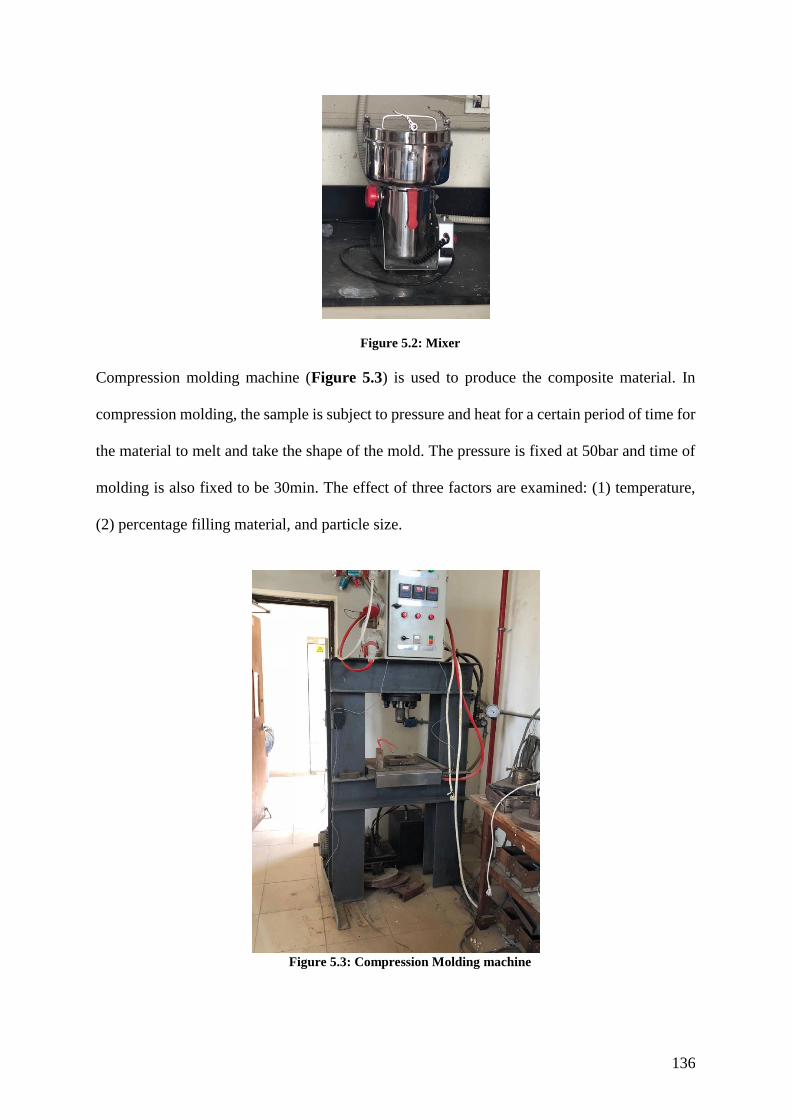
136
Figure 5.2: Mixer
Compression molding machine (Figure 5.3) is used to produce the composite material. In
compression molding, the sample is subject to pressure and heat for a certain period of time for
the material to melt and take the shape of the mold. The pressure is fixed at 50bar and time of
molding is also fixed to be 30min. The effect of three factors are examined: (1) temperature,
(2) percentage filling material, and particle size.
Figure 5.3: Compression Molding machine
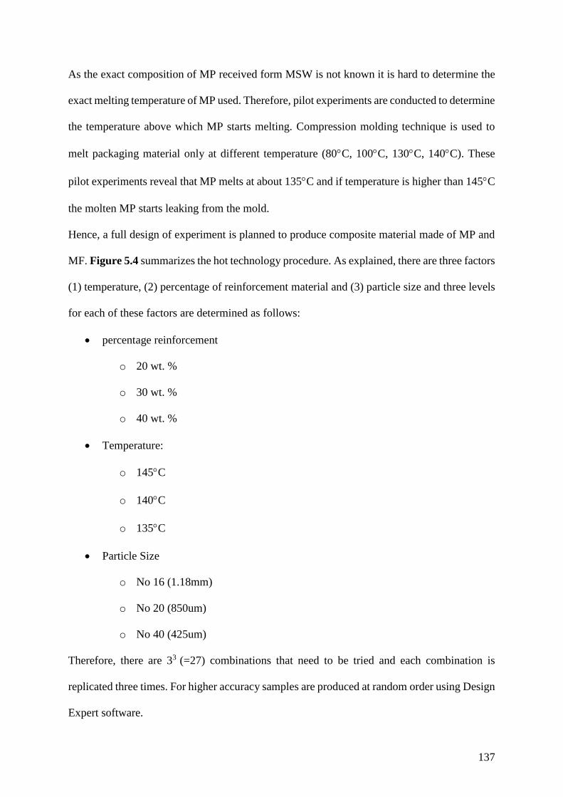
137
As the exact composition of MP received form MSW is not known it is hard to determine the
exact melting temperature of MP used. Therefore, pilot experiments are conducted to determine
the temperature above which MP starts melting. Compression molding technique is used to
melt packaging material only at different temperature (80C, 100C, 130C, 140C). These
pilot experiments reveal that MP melts at about 135C and if temperature is higher than 145C
the molten MP starts leaking from the mold.
Hence, a full design of experiment is planned to produce composite material made of MP and
MF. Figure 5.4 summarizes the hot technology procedure. As explained, there are three factors
(1) temperature, (2) percentage of reinforcement material and (3) particle size and three levels
for each of these factors are determined as follows:
percentage reinforcement
o 20 wt. %
o 30 wt. %
o 40 wt. %
Temperature:
o 145C
o 140C
o 135C
Particle Size
o No 16 (1.18mm)
o No 20 (850um)
o No 40 (425um)
Therefore, there are 33 (=27) combinations that need to be tried and each combination is
replicated three times. For higher accuracy samples are produced at random order using Design
Expert software.
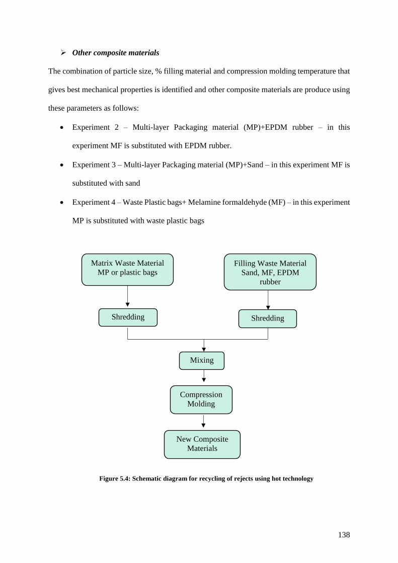
138
Other composite materials
The combination of particle size, % filling material and compression molding temperature that
gives best mechanical properties is identified and other composite materials are produce using
these parameters as follows:
Experiment 2 – Multi-layer Packaging material (MP)+EPDM rubber – in this
experiment MF is substituted with EPDM rubber.
Experiment 3 – Multi-layer Packaging material (MP)+Sand – in this experiment MF is
substituted with sand
Experiment 4 – Waste Plastic bags+ Melamine formaldehyde (MF) – in this experiment
MP is substituted with waste plastic bags
Figure 5.4: Schematic diagram for recycling of rejects using hot technology
New Composite
Materials
Mixing
Compression
Molding
Shredding
Shredding
Matrix Waste Material
MP or plastic bags
Filling Waste Material
Sand, MF, EPDM
rubber
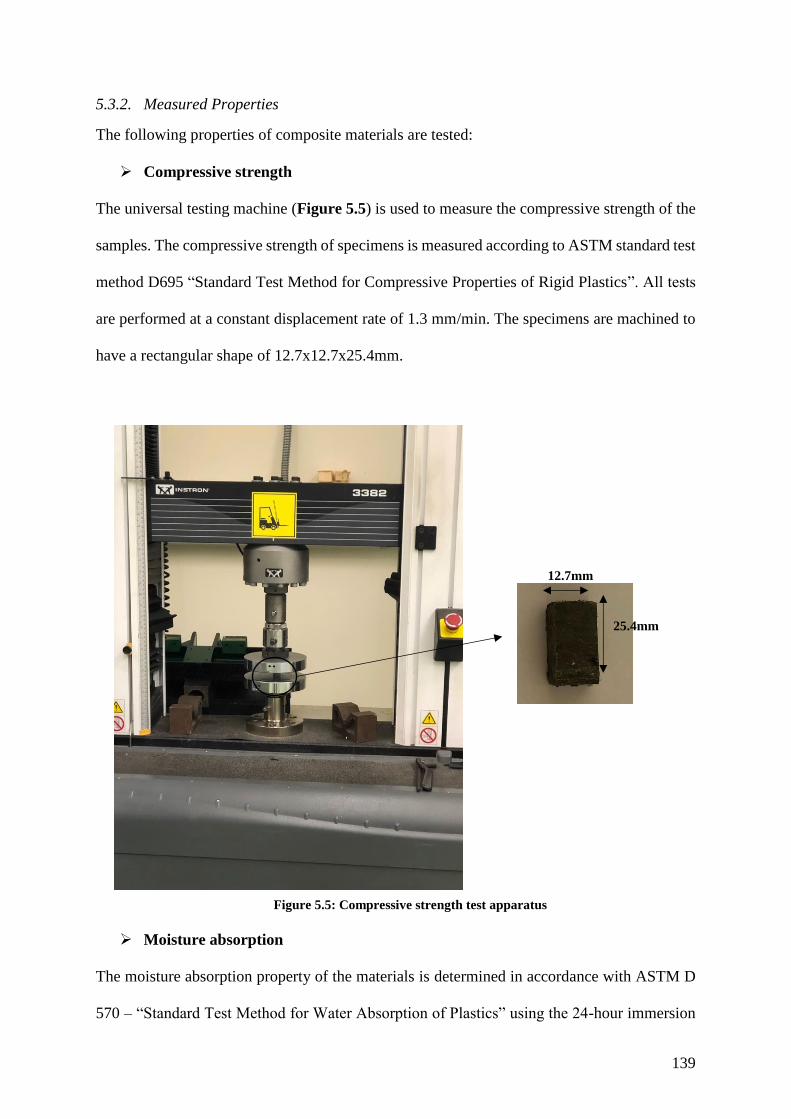
139
5.3.2. Measured Properties
The following properties of composite materials are tested:
Compressive strength
The universal testing machine (Figure 5.5) is used to measure the compressive strength of the
samples. The compressive strength of specimens is measured according to ASTM standard test
method D695 “Standard Test Method for Compressive Properties of Rigid Plastics”. All tests
are performed at a constant displacement rate of 1.3 mm/min. The specimens are machined to
have a rectangular shape of 12.7x12.7x25.4mm.
Figure 5.5: Compressive strength test apparatus
Moisture absorption
The moisture absorption property of the materials is determined in accordance with ASTM D
570 – “Standard Test Method for Water Absorption of Plastics” using the 24-hour immersion
25.4mm
12.7mm
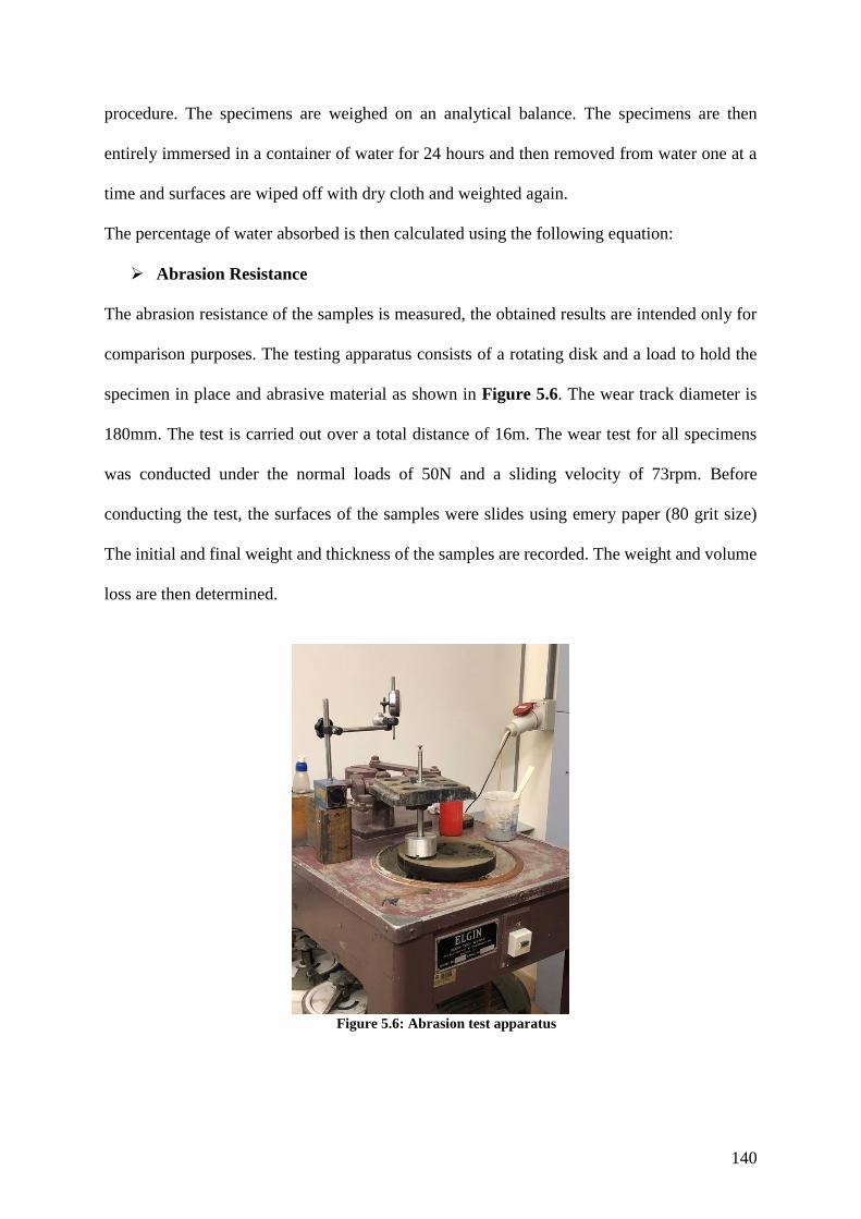
140
procedure. The specimens are weighed on an analytical balance. The specimens are then
entirely immersed in a container of water for 24 hours and then removed from water one at a
time and surfaces are wiped off with dry cloth and weighted again.
The percentage of water absorbed is then calculated using the following equation:
Abrasion Resistance
The abrasion resistance of the samples is measured, the obtained results are intended only for
comparison purposes. The testing apparatus consists of a rotating disk and a load to hold the
specimen in place and abrasive material as shown in Figure 5.6. The wear track diameter is
180mm. The test is carried out over a total distance of 16m. The wear test for all specimens
was conducted under the normal loads of 50N and a sliding velocity of 73rpm. Before
conducting the test, the surfaces of the samples were slides using emery paper (80 grit size)
The initial and final weight and thickness of the samples are recorded. The weight and volume
loss are then determined.
Figure 5.6: Abrasion test apparatus
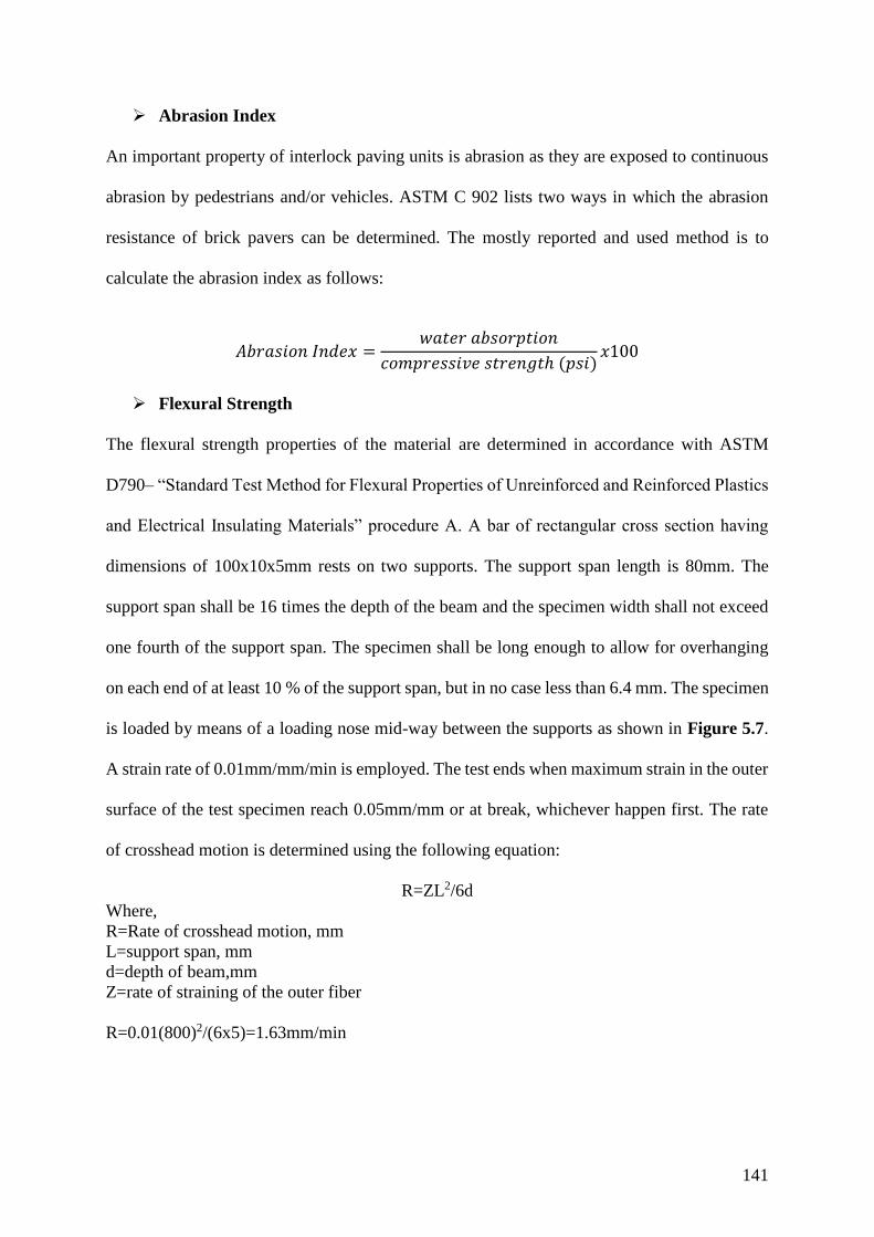
141
Abrasion Index
An important property of interlock paving units is abrasion as they are exposed to continuous
abrasion by pedestrians and/or vehicles. ASTM C 902 lists two ways in which the abrasion
resistance of brick pavers can be determined. The mostly reported and used method is to
calculate the abrasion index as follows:
𝐴𝑏𝑟𝑎𝑠𝑖𝑜𝑛 𝐼𝑛𝑑𝑒𝑥 =𝑤𝑎𝑡𝑒𝑟 𝑎𝑏𝑠𝑜𝑟𝑝𝑡𝑖𝑜𝑛
𝑐𝑜𝑚𝑝𝑟𝑒𝑠𝑠𝑖𝑣𝑒 𝑠𝑡𝑟𝑒𝑛𝑔𝑡ℎ (𝑝𝑠𝑖)𝑥100
Flexural Strength
The flexural strength properties of the material are determined in accordance with ASTM
D790– “Standard Test Method for Flexural Properties of Unreinforced and Reinforced Plastics
and Electrical Insulating Materials” procedure A. A bar of rectangular cross section having
dimensions of 100x10x5mm rests on two supports. The support span length is 80mm. The
support span shall be 16 times the depth of the beam and the specimen width shall not exceed
one fourth of the support span. The specimen shall be long enough to allow for overhanging
on each end of at least 10 % of the support span, but in no case less than 6.4 mm. The specimen
is loaded by means of a loading nose mid-way between the supports as shown in Figure 5.7.
A strain rate of 0.01mm/mm/min is employed. The test ends when maximum strain in the outer
surface of the test specimen reach 0.05mm/mm or at break, whichever happen first. The rate
of crosshead motion is determined using the following equation:
R=ZL2/6d
Where,
R=Rate of crosshead motion, mm
L=support span, mm
d=depth of beam,mm
Z=rate of straining of the outer fiber
R=0.01(800)2/(6x5)=1.63mm/min
142
Figure 5.7: Flexural strength test apparatus
Density
The weight of the specimen is recorded using a digital balance. The specimen dimensions were
geometrically measured to calculate the volume. Density is then calculated by dividing the
specimen’s mass by its volume. The densities of three replicates were measured and the average
was calculated accordingly.
Leachate test
The health hazard of the investigated waste material is determined using the water leaching test
DIN 38414-S4. In this test samples of 15g are immersed in 300ml of deionized water medium
for 28 days. At the end of the immersion period the water is filtered using No. 50 filter paper
and analyzed for the following:
pH using a digital pH meter shown in Figure 5.8
100mm
10mm
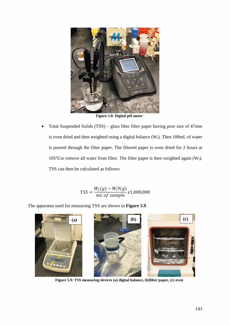
143
Figure 5.8: Digital pH meter
Total Suspended Solids (TSS) – glass fiber filter paper having pore size of 47mm
is oven dried and then weighted using a digital balance (Wi). Then 100mL of water
is poured through the filter paper. The filtered paper is oven dried for 2 hours at
105℃ to remove all water from filter. The filter paper is then weighted again (Wf).
TSS can then be calculated as follows:
𝑇𝑆𝑆 =𝑊𝑓(𝑔) − 𝑊𝑖9(𝑔)
𝑚𝐿 𝑜𝑓 𝑠𝑎𝑚𝑝𝑙𝑒𝑥1,000,000
The apparatus used for measuring TSS are shown in Figure 5.9.
Figure 5.9: TSS measuring devices (a) digital balance, (b)filter paper, (c) oven
(a) (b) (c)
144
Total Dissolved Solids (TDS) is measured using a TDS meter shown in Figure 5.10
Figure 5.10: TDS meter
Nitrate is measured using nitrate method 8039 using Hack DR/ spectrophotometer
2000 (Figure 5.11). A water sample of 25mL is placed inside the spectrophotometer
as a reference. Then another sample is mixed and agitated with reagent for 1 min
then left to react for 5min without agitation, which is then placed inside the
spectrophotometer to take reading of nitrogen (mg/L). Then nitrate is determined
by multiplying the obtained value by 4.4.
Figure 5.11: Nitrate spectrophotometer
Chemical Oxygen Demand (COD) is determined by adding 2mL of water sample
to oxidizing agent (potassium dichromate and sulfuric acid). Then the samples are
145
placed in a reactor for 2hours at 160℃. The samples are then left to cool and a
spectrophotometer shown in Figure 5.12 is used to measure COD.
Figure 5.12: (a) water samples with reagent, (b) COD reactor, (c) Spectrophotometer
Lead (Pb), Chromium (Cr) and cadmium (Cd) are measured suing atomic
absorption spectrometer SensAA shown in Figure 5.13.
Figure 5.13: Atomic absorption spectrometer to measure heavy metals
(b) (c)
(a)
146
5.3.3. Results and discussion
Properties of multi-layer flexible packaging and melamine-formaldehyde (MP+MF)
composite
Compressive strength
The compressive strength was measured for all samples as reported in Table 5.1. Each
sample was tested three times and average value is reported in Table 5.1 and each sample was
replicated three times. The results show that the average compressive strength of all samples
range from 9.09 to 32.54MPa.
Table 5.1: Compressive strength of MP + MF composite material
Specimen
No. % MP % MF
Temp.
(C)
Sieve
No.
Compressive Strength (MPa)
Replicate
1
Replicate
2
Replicate
3 Average
1M 80 20 135 No 16 7.73 9.05 10.98 9.25
2M 70 30 135 No 16 13.21 16.32 11.87 13.80
3M 60 40 135 No 16 12.23 6.34 9.02 9.20
4M 80 20 140 No 16 6.67 10.03 14.02 10.24
5M 70 30 140 No 16 10.04 13.87 18.21 14.04
6M 60 40 140 No 16 9.02 13.21 17.24 13.16
7M 80 20 145 No 16 15.3 19.81 23.08 19.40
8M 70 30 145 No 16 17.94 21.89 26.32 22.05
9M 60 40 145 No 16 13.65 18.76 23.87 18.76
10M 80 20 135 No 20 8.87 13.04 17.08 13.00
11M 70 30 135 No 20 11.34 15.03 18.87 15.08
12M 60 40 135 No 20 10.32 13.87 18.12 14.10
13M 80 20 140 No 20 16.89 22.02 24.95 21.29
14M 70 30 140 No 20 29.67 26.04 20.54 25.42
15M 60 40 140 No 20 14.87 18.84 25.32 19.68
16M 80 20 145 No 20 25.45 29.85 35.03 30.11
17M 70 30 145 No 20 28.54 32.04 37.05 32.54
18M 60 40 145 No 20 15.56 19.86 21.32 18.91
19M 80 20 135 No 40 7.7 11.13 14.74 11.19
20M 70 30 135 No 40 8.4 12.09 15.76 12.08
21M 60 40 135 No 40 5.5 9.45 12.32 9.09
22M 80 20 140 No 40 7.9 11.87 16.59 12.12
23M 70 30 140 No 40 11.34 13.89 18.65 14.63
24M 60 40 140 No 40 9.22 11.53 12.86 11.20
25M 80 20 145 No 40 13.54 17.43 19.67 16.88
26M 70 30 145 No 40 19.54 22.37 24.92 22.28
27M 60 40 145 No 40 13.44 16.98 19.04 16.49
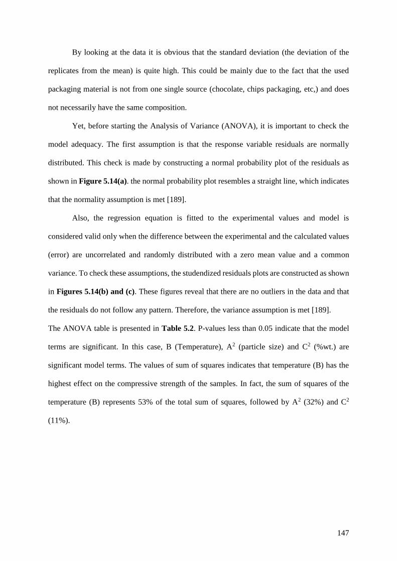
147
By looking at the data it is obvious that the standard deviation (the deviation of the
replicates from the mean) is quite high. This could be mainly due to the fact that the used
packaging material is not from one single source (chocolate, chips packaging, etc,) and does
not necessarily have the same composition.
Yet, before starting the Analysis of Variance (ANOVA), it is important to check the
model adequacy. The first assumption is that the response variable residuals are normally
distributed. This check is made by constructing a normal probability plot of the residuals as
shown in Figure 5.14(a). the normal probability plot resembles a straight line, which indicates
that the normality assumption is met [189].
Also, the regression equation is fitted to the experimental values and model is
considered valid only when the difference between the experimental and the calculated values
(error) are uncorrelated and randomly distributed with a zero mean value and a common
variance. To check these assumptions, the studendized residuals plots are constructed as shown
in Figures 5.14(b) and (c). These figures reveal that there are no outliers in the data and that
the residuals do not follow any pattern. Therefore, the variance assumption is met [189].
The ANOVA table is presented in Table 5.2. P-values less than 0.05 indicate that the model
terms are significant. In this case, B (Temperature), A2 (particle size) and C2 (%wt.) are
significant model terms. The values of sum of squares indicates that temperature (B) has the
highest effect on the compressive strength of the samples. In fact, the sum of squares of the
temperature (B) represents 53% of the total sum of squares, followed by A2 (32%) and C2
(11%).
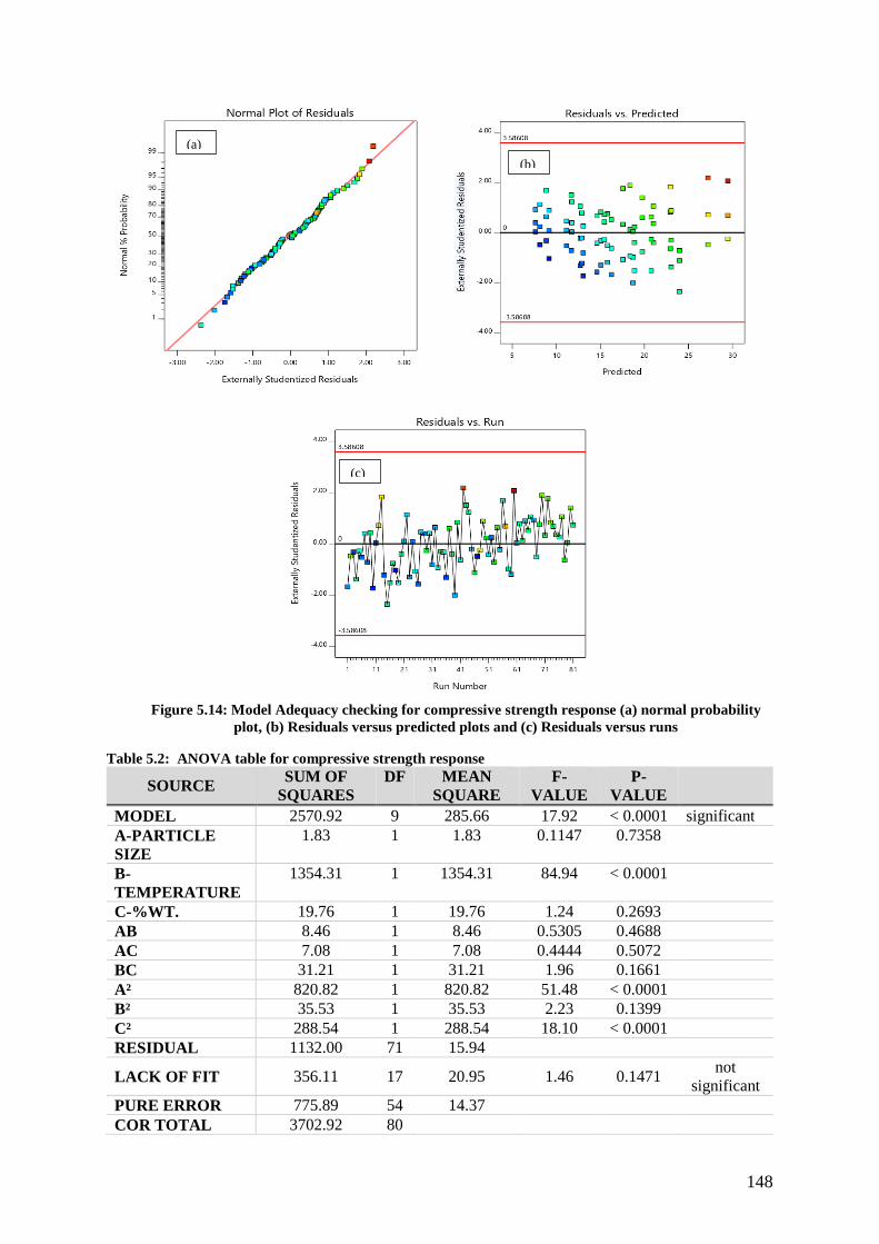
148
Figure 5.14: Model Adequacy checking for compressive strength response (a) normal probability
plot, (b) Residuals versus predicted plots and (c) Residuals versus runs
Table 5.2: ANOVA table for compressive strength response
SOURCE SUM OF
SQUARES
DF MEAN
SQUARE
F-
VALUE
P-
VALUE
MODEL 2570.92 9 285.66 17.92 < 0.0001 significant
A-PARTICLE
SIZE
1.83 1 1.83 0.1147 0.7358
B-
TEMPERATURE
1354.31 1 1354.31 84.94 < 0.0001
C-%WT. 19.76 1 19.76 1.24 0.2693
AB 8.46 1 8.46 0.5305 0.4688
AC 7.08 1 7.08 0.4444 0.5072
BC 31.21 1 31.21 1.96 0.1661
A² 820.82 1 820.82 51.48 < 0.0001
B² 35.53 1 35.53 2.23 0.1399
C² 288.54 1 288.54 18.10 < 0.0001
RESIDUAL 1132.00 71 15.94
LACK OF FIT 356.11 17 20.95 1.46 0.1471 not
significant
PURE ERROR 775.89 54 14.37
COR TOTAL 3702.92 80
(a)
(b)
(c)
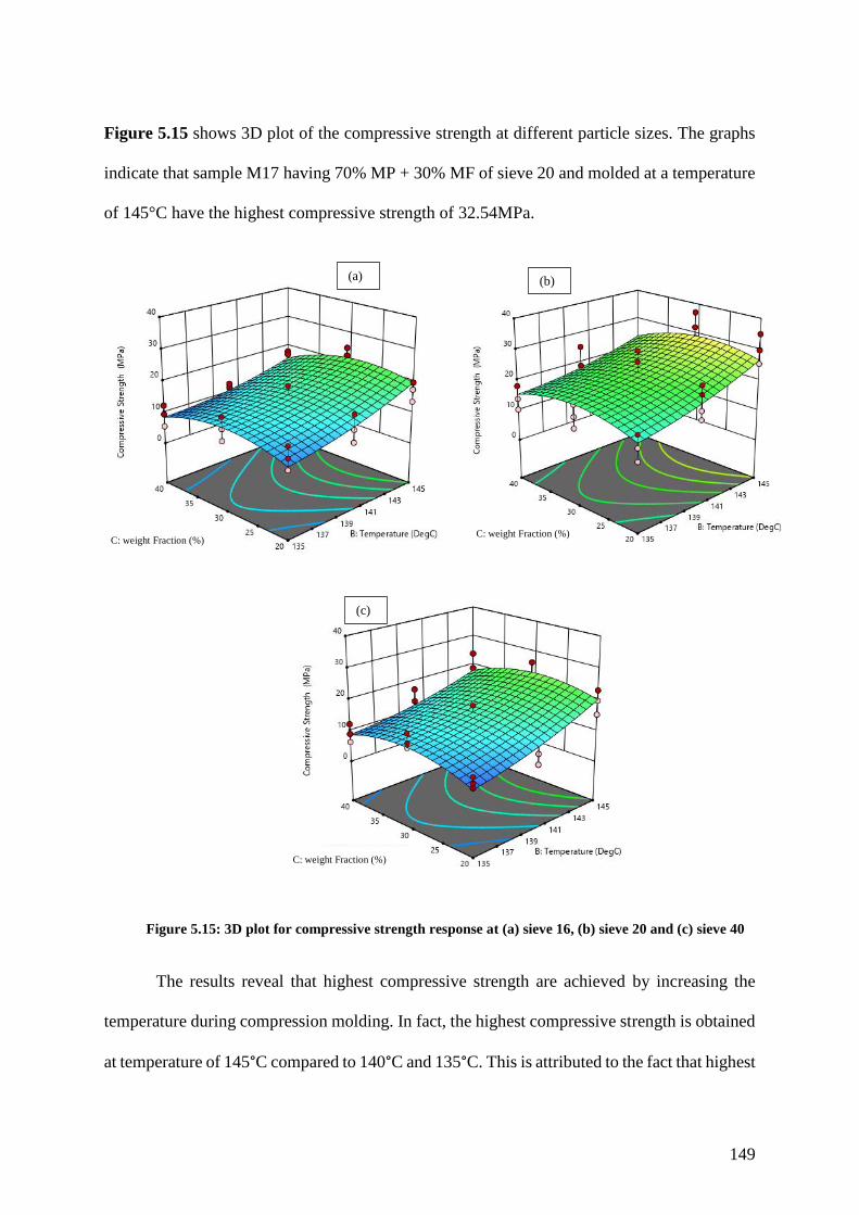
149
Figure 5.15 shows 3D plot of the compressive strength at different particle sizes. The graphs
indicate that sample M17 having 70% MP + 30% MF of sieve 20 and molded at a temperature
of 145°C have the highest compressive strength of 32.54MPa.
Figure 5.15: 3D plot for compressive strength response at (a) sieve 16, (b) sieve 20 and (c) sieve 40
The results reveal that highest compressive strength are achieved by increasing the
temperature during compression molding. In fact, the highest compressive strength is obtained
at temperature of 145°C compared to 140°C and 135°C. This is attributed to the fact that highest
(c)
(a) (b)
C: weight Fraction (%) C: weight Fraction (%)
C: weight Fraction (%)
C: weight Fraction (%) C: weight Fraction (%)
C: weight Fraction (%)
150
temperature allows the packaging material to melt more; therefore, packaging material wet the
filling material more leading to better adhesion between the matrix and filling material.
The results show that there is a relationship between the compressive strength value and
percentage of MF (C2 from the ANOVA table). In fact, the compressive strength increased by
increasing the percentage of MF from 20 to 30%. Many studies have reported that increasing
%wt. improves the mechanical properties of the composite including compressive strength,
tensile strength, fracture toughness, flexural strength etc. [190, 191, 192, 193, 194]. As MF
(filling material) is harder compared to MP (matrix), adding MF to MP improves the strength
of the material. This is due to increase in surface area of contact between the filler and the
matrix, which allows better load transfer from matrix to particles [190]. Also, this observation
agrees with the behavior experienced with filled elastomeric systems, where the filler particles
reinforce the matrix by diverting the path of rupture and hence increasing the energy required
to propagate a crack [5]. The highest compressive strength is observed at 30wt. % of MF.
However, further increase in MF %wt. leads to a decrease in compressive strength. This could
be due to poor adhesive bonding between particles and matrix [190].
Also, the results indicate that the particle size of MF has an effect on compressive
strength (A2 from ANOVA table). In fact, increasing the particle size decreases the
compressive strength. Highest compressive strength values are obtained with sieve 20
compared to sieve 16 and 40. Large particle size (sieve 16-1.18mm) probably act as defects
which leads to localized stress concentration. However, further decrease in particle size from
sieve 20 to 40 cause a decrease in compressive strength. This suggests better dispersion and
wetting characteristics associated with larger filler particles leading to stronger interfacial
bonds. This could be because particles of small sizes form clusters that contain air gaps and
voids and thus are weak points in the material. Also, these clusters usually contain entrapped
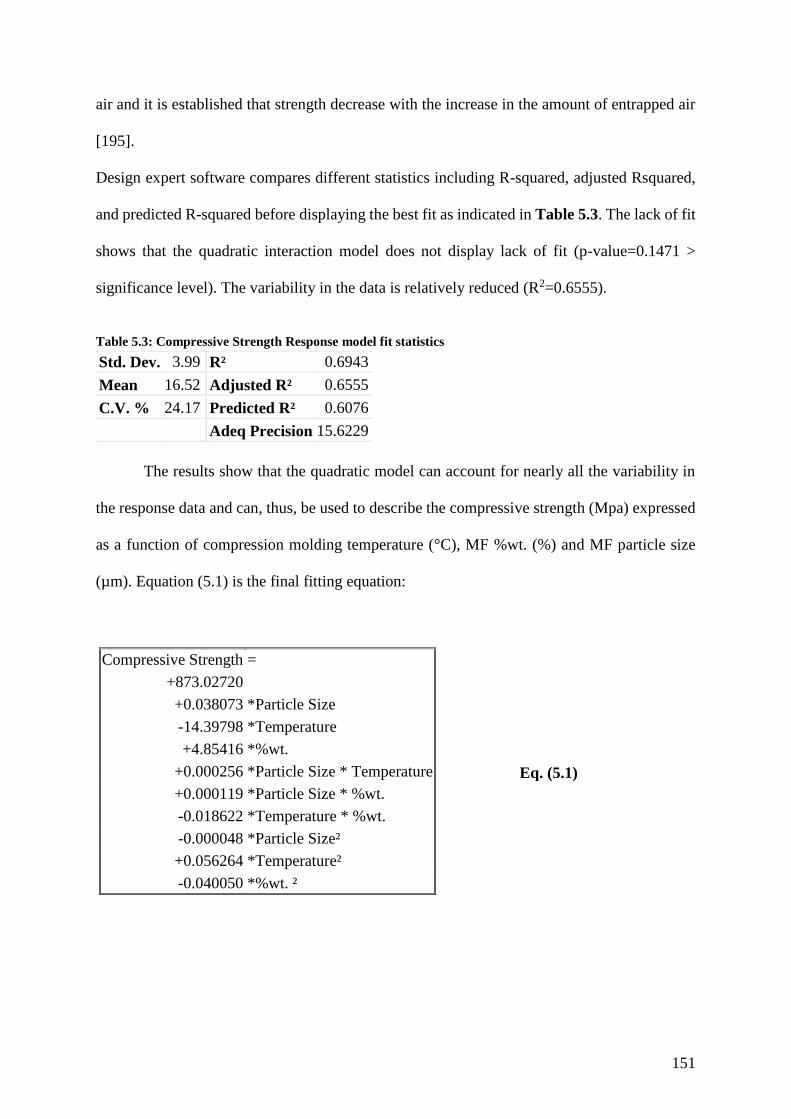
151
air and it is established that strength decrease with the increase in the amount of entrapped air
[195].
Design expert software compares different statistics including R-squared, adjusted Rsquared,
and predicted R-squared before displaying the best fit as indicated in Table 5.3. The lack of fit
shows that the quadratic interaction model does not display lack of fit (p-value=0.1471 >
significance level). The variability in the data is relatively reduced (R2=0.6555).
Table 5.3: Compressive Strength Response model fit statistics
Std. Dev. 3.99 R² 0.6943
Mean 16.52 Adjusted R² 0.6555
C.V. % 24.17 Predicted R² 0.6076 Adeq Precision 15.6229
The results show that the quadratic model can account for nearly all the variability in
the response data and can, thus, be used to describe the compressive strength (Mpa) expressed
as a function of compression molding temperature (°C), MF %wt. (%) and MF particle size
(µm). Equation (5.1) is the final fitting equation:
Compressive Strength =
+873.02720
+0.038073 *Particle Size
-14.39798 *Temperature
+4.85416 *%wt.
+0.000256 *Particle Size * Temperature
+0.000119 *Particle Size * %wt.
-0.018622 *Temperature * %wt.
-0.000048 *Particle Size²
+0.056264 *Temperature²
-0.040050 *%wt. ²
Eq. (5.1)
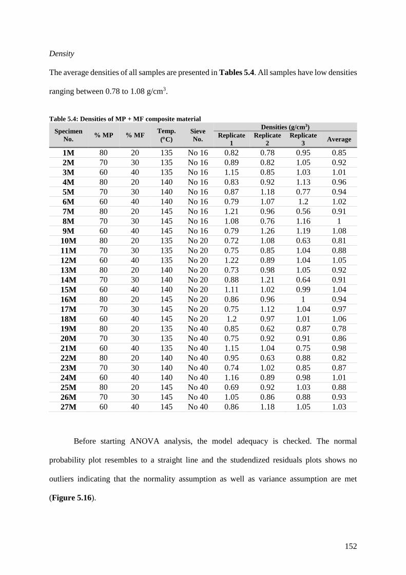
152
Density
The average densities of all samples are presented in Tables 5.4. All samples have low densities
ranging between 0.78 to 1.08 g/cm3.
Table 5.4: Densities of MP + MF composite material
Specimen
No. % MP % MF
Temp.
(C)
Sieve
No.
Densities (g/cm3)
Replicate
1
Replicate
2
Replicate
3 Average
1M 80 20 135 No 16 0.82 0.78 0.95 0.85
2M 70 30 135 No 16 0.89 0.82 1.05 0.92
3M 60 40 135 No 16 1.15 0.85 1.03 1.01
4M 80 20 140 No 16 0.83 0.92 1.13 0.96
5M 70 30 140 No 16 0.87 1.18 0.77 0.94
6M 60 40 140 No 16 0.79 1.07 1.2 1.02
7M 80 20 145 No 16 1.21 0.96 0.56 0.91
8M 70 30 145 No 16 1.08 0.76 1.16 1
9M 60 40 145 No 16 0.79 1.26 1.19 1.08
10M 80 20 135 No 20 0.72 1.08 0.63 0.81
11M 70 30 135 No 20 0.75 0.85 1.04 0.88
12M 60 40 135 No 20 1.22 0.89 1.04 1.05
13M 80 20 140 No 20 0.73 0.98 1.05 0.92
14M 70 30 140 No 20 0.88 1.21 0.64 0.91
15M 60 40 140 No 20 1.11 1.02 0.99 1.04
16M 80 20 145 No 20 0.86 0.96 1 0.94
17M 70 30 145 No 20 0.75 1.12 1.04 0.97
18M 60 40 145 No 20 1.2 0.97 1.01 1.06
19M 80 20 135 No 40 0.85 0.62 0.87 0.78
20M 70 30 135 No 40 0.75 0.92 0.91 0.86
21M 60 40 135 No 40 1.15 1.04 0.75 0.98
22M 80 20 140 No 40 0.95 0.63 0.88 0.82
23M 70 30 140 No 40 0.74 1.02 0.85 0.87
24M 60 40 140 No 40 1.16 0.89 0.98 1.01
25M 80 20 145 No 40 0.69 0.92 1.03 0.88
26M 70 30 145 No 40 1.05 0.86 0.88 0.93
27M 60 40 145 No 40 0.86 1.18 1.05 1.03
Before starting ANOVA analysis, the model adequacy is checked. The normal
probability plot resembles to a straight line and the studendized residuals plots shows no
outliers indicating that the normality assumption as well as variance assumption are met
(Figure 5.16).
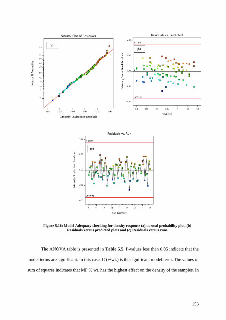
153
Figure 5.16: Model Adequacy checking for density response (a) normal probability plot, (b)
Residuals versus predicted plots and (c) Residuals versus runs
The ANOVA table is presented in Table 5.5. P-values less than 0.05 indicate that the
model terms are significant. In this case, C (%wt.) is the significant model term. The values of
sum of squares indicates that MF % wt. has the highest effect on the density of the samples. In
(c)
(a) (b)
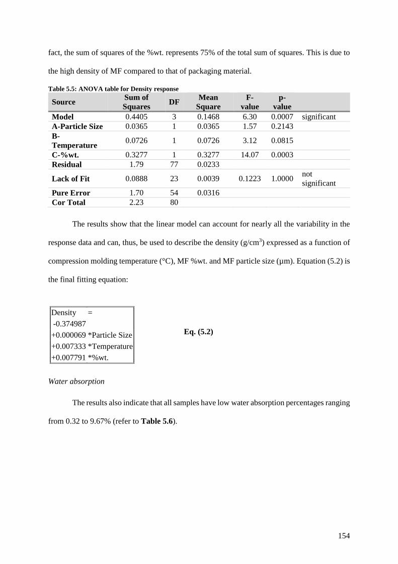
154
fact, the sum of squares of the %wt. represents 75% of the total sum of squares. This is due to
the high density of MF compared to that of packaging material.
Table 5.5: ANOVA table for Density response
Source Sum of
Squares DF
Mean
Square
F-
value
p-
value
Model 0.4405 3 0.1468 6.30 0.0007 significant
A-Particle Size 0.0365 1 0.0365 1.57 0.2143
B-
Temperature 0.0726 1 0.0726 3.12 0.0815
C-%wt. 0.3277 1 0.3277 14.07 0.0003
Residual 1.79 77 0.0233
Lack of Fit 0.0888 23 0.0039 0.1223 1.0000 not
significant
Pure Error 1.70 54 0.0316
Cor Total 2.23 80
The results show that the linear model can account for nearly all the variability in the
response data and can, thus, be used to describe the density (g/cm3) expressed as a function of
compression molding temperature (°C), MF %wt. and MF particle size (µm). Equation (5.2) is
the final fitting equation:
Density =
-0.374987
+0.000069 *Particle Size
+0.007333 *Temperature
+0.007791 *%wt.
Water absorption
The results also indicate that all samples have low water absorption percentages ranging
from 0.32 to 9.67% (refer to Table 5.6).
Eq. (5.2)
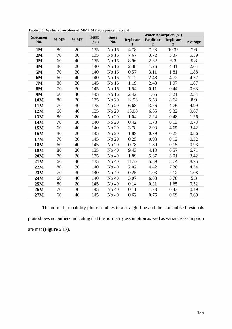
155
Table 5.6: Water absorption of MP + MF composite material
Specimen
No. % MP % MF
Temp.
(C)
Sieve
No.
Water Absorption (%)
Replicate
1
Replicate
2
Replicate
3 Average
1M 80 20 135 No 16 4.78 7.23 10.32 7.6
2M 70 30 135 No 16 7.67 3.72 5.37 5.59
3M 60 40 135 No 16 8.96 2.32 6.3 5.8
4M 80 20 140 No 16 2.38 1.26 4.41 2.64
5M 70 30 140 No 16 0.57 3.11 1.81 1.88
6M 60 40 140 No 16 7.12 2.48 4.72 4.77
7M 80 20 145 No 16 1.19 2.43 1.97 1.87
8M 70 30 145 No 16 1.54 0.11 0.44 0.63
9M 60 40 145 No 16 2.42 1.65 3.21 2.34
10M 80 20 135 No 20 12.53 5.53 8.64 8.9
11M 70 30 135 No 20 6.68 3.76 4.76 4.99
12M 60 40 135 No 20 13.08 6.65 9.32 9.67
13M 80 20 140 No 20 1.04 2.24 0.48 1.26
14M 70 30 140 No 20 0.42 1.78 0.13 0.73
15M 60 40 140 No 20 3.78 2.03 4.65 3.42
16M 80 20 145 No 20 1.89 0.79 0.23 0.86
17M 70 30 145 No 20 0.25 0.98 0.12 0.32
18M 60 40 145 No 20 0.78 1.89 0.15 0.93
19M 80 20 135 No 40 9.43 4.13 6.57 6.71
20M 70 30 135 No 40 1.89 5.67 3.01 3.42
21M 60 40 135 No 40 11.52 5.89 8.74 8.75
22M 80 20 140 No 40 2.02 4.42 7.28 4.34
23M 70 30 140 No 40 0.25 1.03 2.12 1.08
24M 60 40 140 No 40 3.07 6.88 5.78 5.3
25M 80 20 145 No 40 0.14 0.21 1.65 0.52
26M 70 30 145 No 40 0.11 1.23 0.43 0.49
27M 60 40 145 No 40 0.62 0.76 0.69 0.69
The normal probability plot resembles to a straight line and the studendized residuals
plots shows no outliers indicating that the normality assumption as well as variance assumption
are met (Figure 5.17).

156
Figure 5.17: Model Adequacy checking for water absorption response (a) normal probability plot,
(b) Residuals versus predicted plots and (c) Residuals versus runs
The ANOVA table is presented in Table 5.7. P-values less than 0.05 indicate that the
model terms are significant. In this case, B (Temperature), B2 and C2(%wt.) are significant
model terms. The values of sum of squares indicates that compression molding temperature
(B) has the highest effect on the water absorption of the samples. In fact, the sum of squares of
the temperature represents 80% of the total sum of squares.
(a)
(b)
(c)
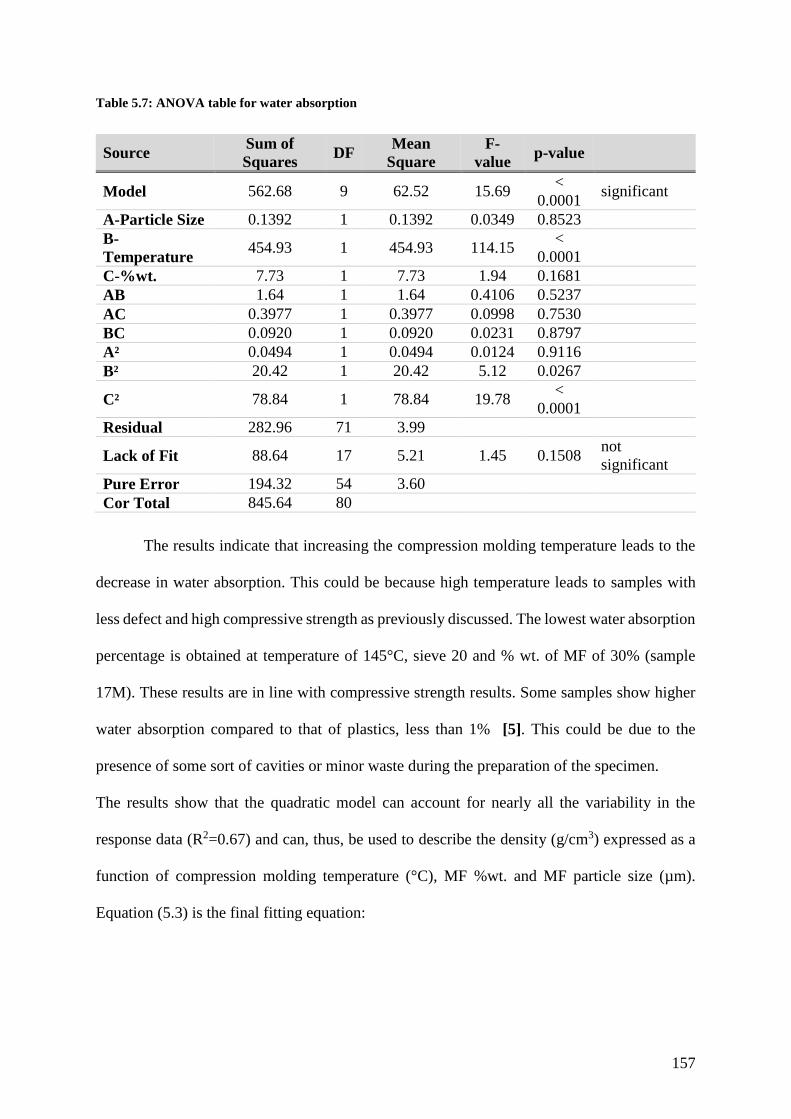
157
Table 5.7: ANOVA table for water absorption
Source Sum of
Squares DF
Mean
Square
F-
value p-value
Model 562.68 9 62.52 15.69 <
0.0001 significant
A-Particle Size 0.1392 1 0.1392 0.0349 0.8523
B-
Temperature 454.93 1 454.93 114.15
<
0.0001
C-%wt. 7.73 1 7.73 1.94 0.1681
AB 1.64 1 1.64 0.4106 0.5237
AC 0.3977 1 0.3977 0.0998 0.7530
BC 0.0920 1 0.0920 0.0231 0.8797
A² 0.0494 1 0.0494 0.0124 0.9116
B² 20.42 1 20.42 5.12 0.0267
C² 78.84 1 78.84 19.78 <
0.0001
Residual 282.96 71 3.99
Lack of Fit 88.64 17 5.21 1.45 0.1508 not
significant
Pure Error 194.32 54 3.60
Cor Total 845.64 80
The results indicate that increasing the compression molding temperature leads to the
decrease in water absorption. This could be because high temperature leads to samples with
less defect and high compressive strength as previously discussed. The lowest water absorption
percentage is obtained at temperature of 145°C, sieve 20 and % wt. of MF of 30% (sample
17M). These results are in line with compressive strength results. Some samples show higher
water absorption compared to that of plastics, less than 1% [5]. This could be due to the
presence of some sort of cavities or minor waste during the preparation of the specimen.
The results show that the quadratic model can account for nearly all the variability in the
response data (R2=0.67) and can, thus, be used to describe the density (g/cm3) expressed as a
function of compression molding temperature (°C), MF %wt. and MF particle size (µm).
Equation (5.3) is the final fitting equation:
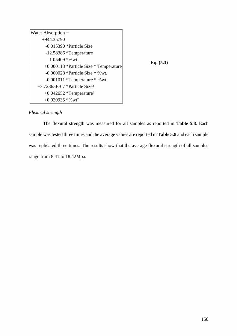
158
Water Absorption =
+944.35790
-0.015390 *Particle Size
-12.58386 *Temperature
-1.05409 *%wt.
+0.000113 *Particle Size * Temperature
-0.000028 *Particle Size * %wt.
-0.001011 *Temperature * %wt.
+3.72365E-07 *Particle Size²
+0.042652 *Temperature²
+0.020935 *%wt²
Flexural strength
The flexural strength was measured for all samples as reported in Table 5.8. Each
sample was tested three times and the average values are reported in Table 5.8 and each sample
was replicated three times. The results show that the average flexural strength of all samples
range from 8.41 to 18.42Mpa.
Eq. (5.3)
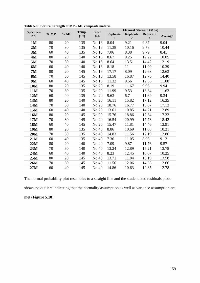
159
Table 5.8: Flexural Strength of MP – MF composite material
Specimen
No. % MP % MF
Temp.
(C)
Sieve
No.
Flexural Strength (Mpa)
Replicate
1
Replicate
2
Replicate
3 Average
1M 80 20 135 No 16 8.04 9.21 9.87 9.04
2M 70 30 135 No 16 11.38 10.16 9.78 10.44
3M 60 40 135 No 16 7.06 8.38 9.79 8.41
4M 80 20 140 No 16 8.67 9.25 12.22 10.05
5M 70 30 140 No 16 8.64 13.51 14.42 12.19
6M 60 40 140 No 16 8.18 11 11.99 10.39
7M 80 20 145 No 16 17.17 8.09 12.63 12.63
8M 70 30 145 No 16 13.58 16.87 12.76 14.40
9M 60 40 145 No 16 11.32 9.56 12.36 11.08
10M 80 20 135 No 20 8.19 11.67 9.96 9.94
11M 70 30 135 No 20 11.99 9.53 13.34 11.62
12M 60 40 135 No 20 9.63 6.7 11.69 9.34
13M 80 20 140 No 20 16.11 15.82 17.12 16.35
14M 70 30 140 No 20 18.76 16.77 15.87 17.13
15M 60 40 140 No 20 13.61 10.85 14.21 12.89
16M 80 20 145 No 20 15.76 18.86 17.34 17.32
17M 70 30 145 No 20 16.54 20.99 17.73 18.42
18M 60 40 145 No 20 15.47 11.81 14.46 13.91
19M 80 20 135 No 40 8.86 10.69 11.08 10.21
20M 70 30 135 No 40 14.83 11.56 12.19 12.86
21M 60 40 135 No 40 7.36 11.05 8.95 9.12
22M 80 20 140 No 40 7.09 9.87 11.76 9.57
23M 70 30 140 No 40 13.24 12.89 15.21 13.78
24M 60 40 140 No 40 8.23 12.45 10.07 10.25
25M 80 20 145 No 40 13.71 11.84 15.19 13.58
26M 70 30 145 No 40 11.56 12.06 14.35 12.66
27M 60 40 145 No 40 14.86 10.63 12.85 12.78
The normal probability plot resembles to a straight line and the studendized residuals plots
shows no outliers indicating that the normality assumption as well as variance assumption are
met (Figure 5.18).

160
Figure 5.18: Model Adequacy checking for flexural strength response (a) normal probability plot,
(b) Residuals versus predicted plots and (c) Residuals versus runs
The ANOVA table is presented in table 5.9. P-values less than 0.05 indicate that the model
terms are significant. In this case, B (Temperature), A2 (particle size) and C2 (%wt.). The values
of sum of squares indicates that compression molding temperature (B) has the highest effect
on the flexural strength of the samples. In fact, the sum of squares of the temperature represents
44% of the total sum of squares.
(a)
(b)
(b)
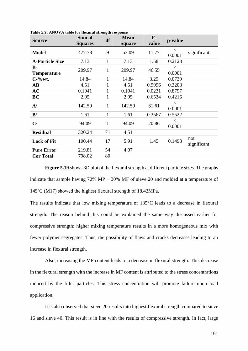
161
Table 5.9: ANOVA table for flexural strength response
Source Sum of
Squares df
Mean
Square
F-
value p-value
Model 477.78 9 53.09 11.77 <
0.0001 significant
A-Particle Size 7.13 1 7.13 1.58 0.2128
B-
Temperature 209.97 1 209.97 46.55
<
0.0001
C-%wt. 14.84 1 14.84 3.29 0.0739
AB 4.51 1 4.51 0.9996 0.3208
AC 0.1041 1 0.1041 0.0231 0.8797
BC 2.95 1 2.95 0.6534 0.4216
A² 142.59 1 142.59 31.61 <
0.0001
B² 1.61 1 1.61 0.3567 0.5522
C² 94.09 1 94.09 20.86 <
0.0001
Residual 320.24 71 4.51
Lack of Fit 100.44 17 5.91 1.45 0.1498 not
significant
Pure Error 219.81 54 4.07
Cor Total 798.02 80
Figure 5.19 shows 3D plot of the flexural strength at different particle sizes. The graphs
indicate that sample having 70% MP + 30% MF of sieve 20 and molded at a temperature of
145°C (M17) showed the highest flexural strength of 18.42MPa.
The results indicate that low mixing temperature of 135°C leads to a decrease in flexural
strength. The reason behind this could be explained the same way discussed earlier for
compressive strength; higher mixing temperature results in a more homogeneous mix with
fewer polymer segregates. Thus, the possibility of flaws and cracks decreases leading to an
increase in flexural strength.
Also, increasing the MF content leads to a decrease in flexural strength. This decrease
in the flexural strength with the increase in MF content is attributed to the stress concentrations
induced by the filler particles. This stress concentration will promote failure upon load
application.
It is also observed that sieve 20 results into highest flexural strength compared to sieve
16 and sieve 40. This result is in line with the results of compressive strength. In fact, large
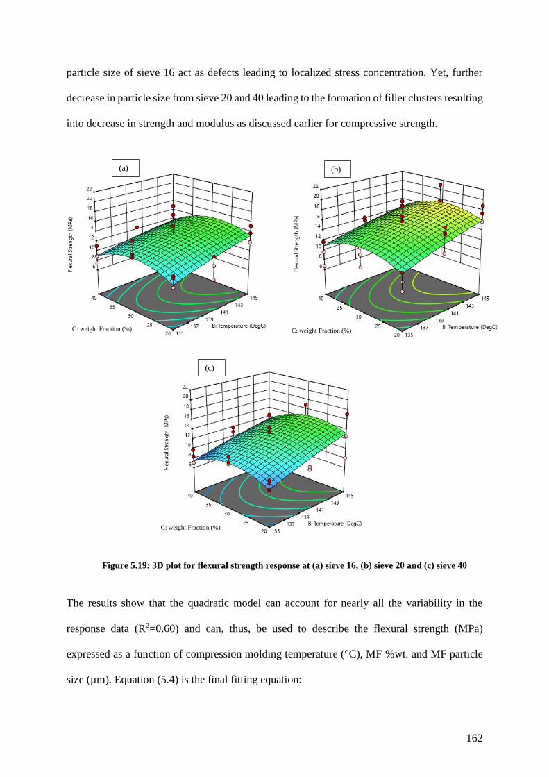
162
particle size of sieve 16 act as defects leading to localized stress concentration. Yet, further
decrease in particle size from sieve 20 and 40 leading to the formation of filler clusters resulting
into decrease in strength and modulus as discussed earlier for compressive strength.
Figure 5.19: 3D plot for flexural strength response at (a) sieve 16, (b) sieve 20 and (c) sieve 40
The results show that the quadratic model can account for nearly all the variability in the
response data (R2=0.60) and can, thus, be used to describe the flexural strength (MPa)
expressed as a function of compression molding temperature (°C), MF %wt. and MF particle
size (µm). Equation (5.4) is the final fitting equation:
(a) (b)
(c)
C: weight Fraction (%) C: weight Fraction (%)
C: weight Fraction (%)
163
Abrasion Resistance
The abrasion resistance of all samples is measured, and results are presented in Table
5.10. The obtained results are intended only for comparison purposes. The lowest value is
obtained for the sample molded at temperature of 145°C and containing 30 % wt. of sieve 20
MF (sample 17M). These results are in line with the compressive and flexural strength results.
Low abrasion thickness losses are observed at high molding temperature, MF sieve 20 and
moderate MF content. This is contributed to the fact that these conditions lead to strong
adhesive bond between filling material and packaging material as discussed earlier in
compressive and flexural strength.
Flexural Strength =
-308.58995
+0.005375 Particle Size
+3.76907 Temperature
+2.13239 %wt.
+0.000187 Particle Size * Temperature
-0.000014 Particle Size * %wt.
-0.005722 Temperature * %wt.
-0.000020 Particle Size²
-0.011973 Temperature²
-0.022870 %wt.²
Eq. (5.4)
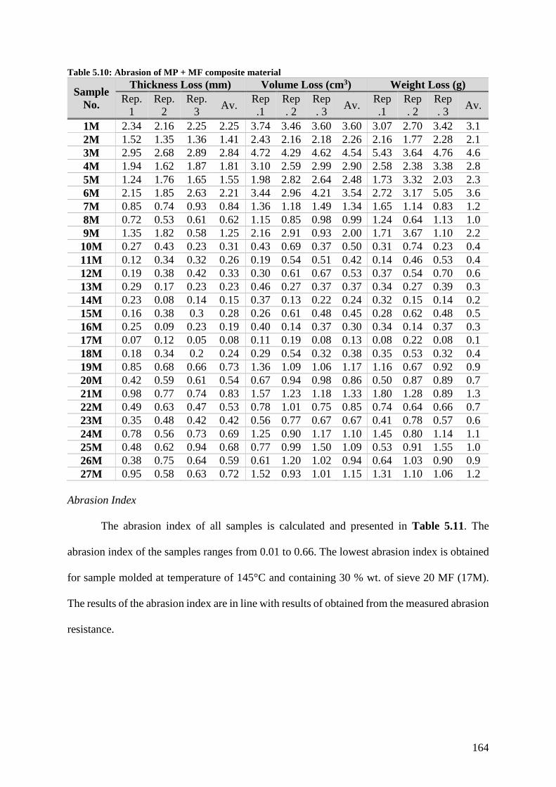
164
Table 5.10: Abrasion of MP + MF composite material
Sample
No.
Thickness Loss (mm) Volume Loss (cm3) Weight Loss (g)
Rep.
1
Rep.
2
Rep.
3 Av.
Rep
.1
Rep
. 2
Rep
. 3 Av.
Rep
.1
Rep
. 2
Rep
. 3 Av.
1M 2.34 2.16 2.25 2.25 3.74 3.46 3.60 3.60 3.07 2.70 3.42 3.1
2M 1.52 1.35 1.36 1.41 2.43 2.16 2.18 2.26 2.16 1.77 2.28 2.1
3M 2.95 2.68 2.89 2.84 4.72 4.29 4.62 4.54 5.43 3.64 4.76 4.6
4M 1.94 1.62 1.87 1.81 3.10 2.59 2.99 2.90 2.58 2.38 3.38 2.8
5M 1.24 1.76 1.65 1.55 1.98 2.82 2.64 2.48 1.73 3.32 2.03 2.3
6M 2.15 1.85 2.63 2.21 3.44 2.96 4.21 3.54 2.72 3.17 5.05 3.6
7M 0.85 0.74 0.93 0.84 1.36 1.18 1.49 1.34 1.65 1.14 0.83 1.2
8M 0.72 0.53 0.61 0.62 1.15 0.85 0.98 0.99 1.24 0.64 1.13 1.0
9M 1.35 1.82 0.58 1.25 2.16 2.91 0.93 2.00 1.71 3.67 1.10 2.2
10M 0.27 0.43 0.23 0.31 0.43 0.69 0.37 0.50 0.31 0.74 0.23 0.4
11M 0.12 0.34 0.32 0.26 0.19 0.54 0.51 0.42 0.14 0.46 0.53 0.4
12M 0.19 0.38 0.42 0.33 0.30 0.61 0.67 0.53 0.37 0.54 0.70 0.6
13M 0.29 0.17 0.23 0.23 0.46 0.27 0.37 0.37 0.34 0.27 0.39 0.3
14M 0.23 0.08 0.14 0.15 0.37 0.13 0.22 0.24 0.32 0.15 0.14 0.2
15M 0.16 0.38 0.3 0.28 0.26 0.61 0.48 0.45 0.28 0.62 0.48 0.5
16M 0.25 0.09 0.23 0.19 0.40 0.14 0.37 0.30 0.34 0.14 0.37 0.3
17M 0.07 0.12 0.05 0.08 0.11 0.19 0.08 0.13 0.08 0.22 0.08 0.1
18M 0.18 0.34 0.2 0.24 0.29 0.54 0.32 0.38 0.35 0.53 0.32 0.4
19M 0.85 0.68 0.66 0.73 1.36 1.09 1.06 1.17 1.16 0.67 0.92 0.9
20M 0.42 0.59 0.61 0.54 0.67 0.94 0.98 0.86 0.50 0.87 0.89 0.7
21M 0.98 0.77 0.74 0.83 1.57 1.23 1.18 1.33 1.80 1.28 0.89 1.3
22M 0.49 0.63 0.47 0.53 0.78 1.01 0.75 0.85 0.74 0.64 0.66 0.7
23M 0.35 0.48 0.42 0.42 0.56 0.77 0.67 0.67 0.41 0.78 0.57 0.6
24M 0.78 0.56 0.73 0.69 1.25 0.90 1.17 1.10 1.45 0.80 1.14 1.1
25M 0.48 0.62 0.94 0.68 0.77 0.99 1.50 1.09 0.53 0.91 1.55 1.0
26M 0.38 0.75 0.64 0.59 0.61 1.20 1.02 0.94 0.64 1.03 0.90 0.9
27M 0.95 0.58 0.63 0.72 1.52 0.93 1.01 1.15 1.31 1.10 1.06 1.2
Abrasion Index
The abrasion index of all samples is calculated and presented in Table 5.11. The
abrasion index of the samples ranges from 0.01 to 0.66. The lowest abrasion index is obtained
for sample molded at temperature of 145°C and containing 30 % wt. of sieve 20 MF (17M).
The results of the abrasion index are in line with results of obtained from the measured abrasion
resistance.
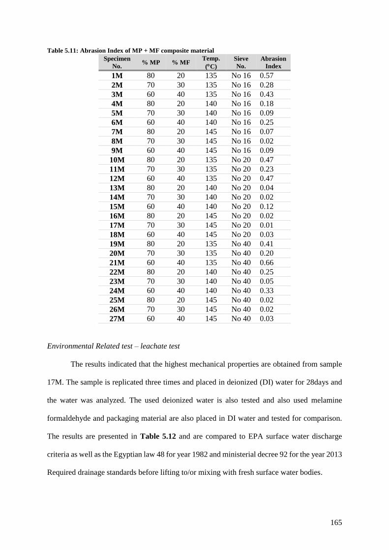
165
Table 5.11: Abrasion Index of MP + MF composite material
Specimen
No. % MP % MF
Temp.
(C)
Sieve
No.
Abrasion
Index
1M 80 20 135 No 16 0.57
2M 70 30 135 No 16 0.28
3M 60 40 135 No 16 0.43
4M 80 20 140 No 16 0.18
5M 70 30 140 No 16 0.09
6M 60 40 140 No 16 0.25
7M 80 20 145 No 16 0.07
8M 70 30 145 No 16 0.02
9M 60 40 145 No 16 0.09
10M 80 20 135 No 20 0.47
11M 70 30 135 No 20 0.23
12M 60 40 135 No 20 0.47
13M 80 20 140 No 20 0.04
14M 70 30 140 No 20 0.02
15M 60 40 140 No 20 0.12
16M 80 20 145 No 20 0.02
17M 70 30 145 No 20 0.01
18M 60 40 145 No 20 0.03
19M 80 20 135 No 40 0.41
20M 70 30 135 No 40 0.20
21M 60 40 135 No 40 0.66
22M 80 20 140 No 40 0.25
23M 70 30 140 No 40 0.05
24M 60 40 140 No 40 0.33
25M 80 20 145 No 40 0.02
26M 70 30 145 No 40 0.02
27M 60 40 145 No 40 0.03
Environmental Related test – leachate test
The results indicated that the highest mechanical properties are obtained from sample
17M. The sample is replicated three times and placed in deionized (DI) water for 28days and
the water was analyzed. The used deionized water is also tested and also used melamine
formaldehyde and packaging material are also placed in DI water and tested for comparison.
The results are presented in Table 5.12 and are compared to EPA surface water discharge
criteria as well as the Egyptian law 48 for year 1982 and ministerial decree 92 for the year 2013
Required drainage standards before lifting to/or mixing with fresh surface water bodies.
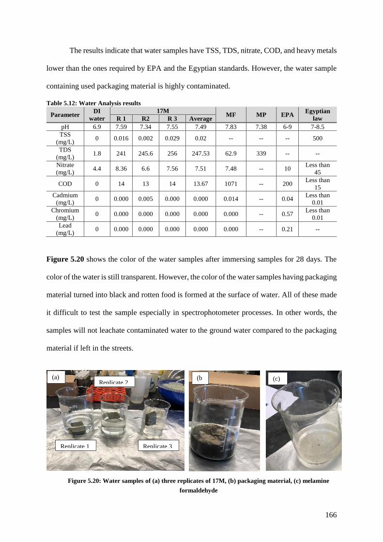
166
The results indicate that water samples have TSS, TDS, nitrate, COD, and heavy metals
lower than the ones required by EPA and the Egyptian standards. However, the water sample
containing used packaging material is highly contaminated.
Table 5.12: Water Analysis results
Parameter DI
water
17M MF MP EPA
Egyptian
law R 1 R2 R 3 Average
pH 6.9 7.59 7.34 7.55 7.49 7.83 7.38 6-9 7-8.5
TSS
(mg/L) 0 0.016 0.002 0.029 0.02 -- -- -- 500
TDS
(mg/L) 1.8 241 245.6 256 247.53 62.9 339 -- --
Nitrate
(mg/L) 4.4 8.36 6.6 7.56 7.51 7.48 -- 10
Less than
45
COD 0 14 13 14 13.67 1071 -- 200 Less than
15
Cadmium
(mg/L) 0 0.000 0.005 0.000 0.000 0.014 -- 0.04
Less than
0.01
Chromium
(mg/L) 0 0.000 0.000 0.000 0.000 0.000 -- 0.57
Less than
0.01
Lead
(mg/L) 0 0.000 0.000 0.000 0.000 0.000 -- 0.21 --
Figure 5.20 shows the color of the water samples after immersing samples for 28 days. The
color of the water is still transparent. However, the color of the water samples having packaging
material turned into black and rotten food is formed at the surface of water. All of these made
it difficult to test the sample especially in spectrophotometer processes. In other words, the
samples will not leachate contaminated water to the ground water compared to the packaging
material if left in the streets.
Figure 5.20: Water samples of (a) three replicates of 17M, (b) packaging material, (c) melamine
formaldehyde
Replicate 2
Replicate 1 Replicate 3
(b
) (c) (a)
167
The results indicate that water samples are within required EPA and Egyptian law limits
for discharged on surface water.
Conclusion of MP+MF composite experiment
A full design of experiment was conducted to study the effect of different compression
molding parameters (temperature, %wt. fraction of filling and particle size of filling material.
The results indicated that highest mechanical properties are obtained using molding
temperature of 145C, sieve 20 and 30%wt.
Recycling of alternative rejects
Based on the results obtained with MP+MF composite material, the best results are
obtained using molding temperature of 145C, sieve 20 and 30%wt. fraction of MF. These
conditions are used to produce other composite materials as follows:
Multi-layer Packaging material (MP)+EPDM rubber – in this experiment MF is
substituted with EPDM rubber
Multi-layer Packaging material (MP)+Sand – in this experiment MF is substituted with
sand
Waste Plastic bags (PB)+ Melamine formaldehyde (MF) – in this experiment MP is
substituted with waste plastic bags
Table 5.13 summarizes the results for the three composites listed above. The values presented
in the table are average of three replicates.
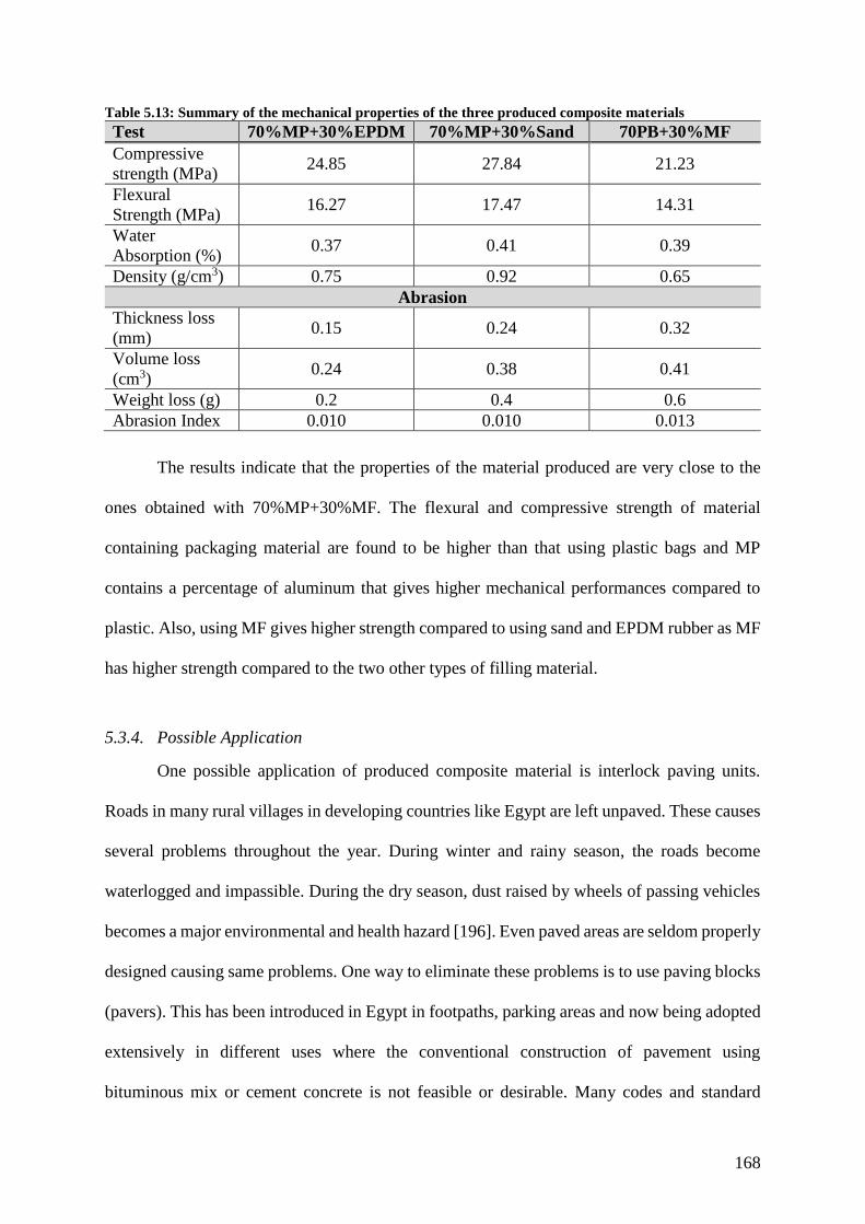
168
Table 5.13: Summary of the mechanical properties of the three produced composite materials
Test 70%MP+30%EPDM 70%MP+30%Sand 70PB+30%MF
Compressive
strength (MPa) 24.85 27.84 21.23
Flexural
Strength (MPa) 16.27 17.47 14.31
Water
Absorption (%) 0.37 0.41 0.39
Density (g/cm3) 0.75 0.92 0.65
Abrasion
Thickness loss
(mm) 0.15 0.24 0.32
Volume loss
(cm3) 0.24 0.38 0.41
Weight loss (g) 0.2 0.4 0.6
Abrasion Index 0.010 0.010 0.013
The results indicate that the properties of the material produced are very close to the
ones obtained with 70%MP+30%MF. The flexural and compressive strength of material
containing packaging material are found to be higher than that using plastic bags and MP
contains a percentage of aluminum that gives higher mechanical performances compared to
plastic. Also, using MF gives higher strength compared to using sand and EPDM rubber as MF
has higher strength compared to the two other types of filling material.
5.3.4. Possible Application
One possible application of produced composite material is interlock paving units.
Roads in many rural villages in developing countries like Egypt are left unpaved. These causes
several problems throughout the year. During winter and rainy season, the roads become
waterlogged and impassible. During the dry season, dust raised by wheels of passing vehicles
becomes a major environmental and health hazard [196]. Even paved areas are seldom properly
designed causing same problems. One way to eliminate these problems is to use paving blocks
(pavers). This has been introduced in Egypt in footpaths, parking areas and now being adopted
extensively in different uses where the conventional construction of pavement using
bituminous mix or cement concrete is not feasible or desirable. Many codes and standard
169
sallow the use of recycled material in the interlock production [197]. Several researchers have
studied the use of waste materials in concrete such as coal, fly ash, plastic waste, industrial
waste fiber, rubber pads, marbles etc. The use of recycled material allows to reduce the cost of
final product as well as conserve natural resources. According to ASTM standards there are
two major classifications of interlocks (1) Pedestrian and Light Traffic Paving Brick (ASTM
C902) and (2) Heavy Vehicular Paving Brick each one has several sub-classifications (ASTM
C1272). This research focuses on Pedestrian and Light Traffic Paving Brick, which can be sub-
divided into other classifications based on the type of weather and traffic as follows:
Weather:
o SX – Brick that maybe frozen while saturated with water
o MX – Brick intended for exterior with no freezing conditions
o NX – Brick intended for interior use with no freezing conditions
Traffic:
o Type I – Pavers subjected to extensive abrasion, such as public sidewalks
and driveways
o Type II – Pavers subjected to intermediate abrasion, such as residential
walkways and residential driveways
o Type III – Pavers subjected to low abrasion, such as floors or patios in single
family Homes
According to ASTM specification C902 -15 – Standard Specification for Pedestrian and Light
Traffic Paving Brick – the acceptable properties for interlocks are summarized in Table 5.14
and 5.15.
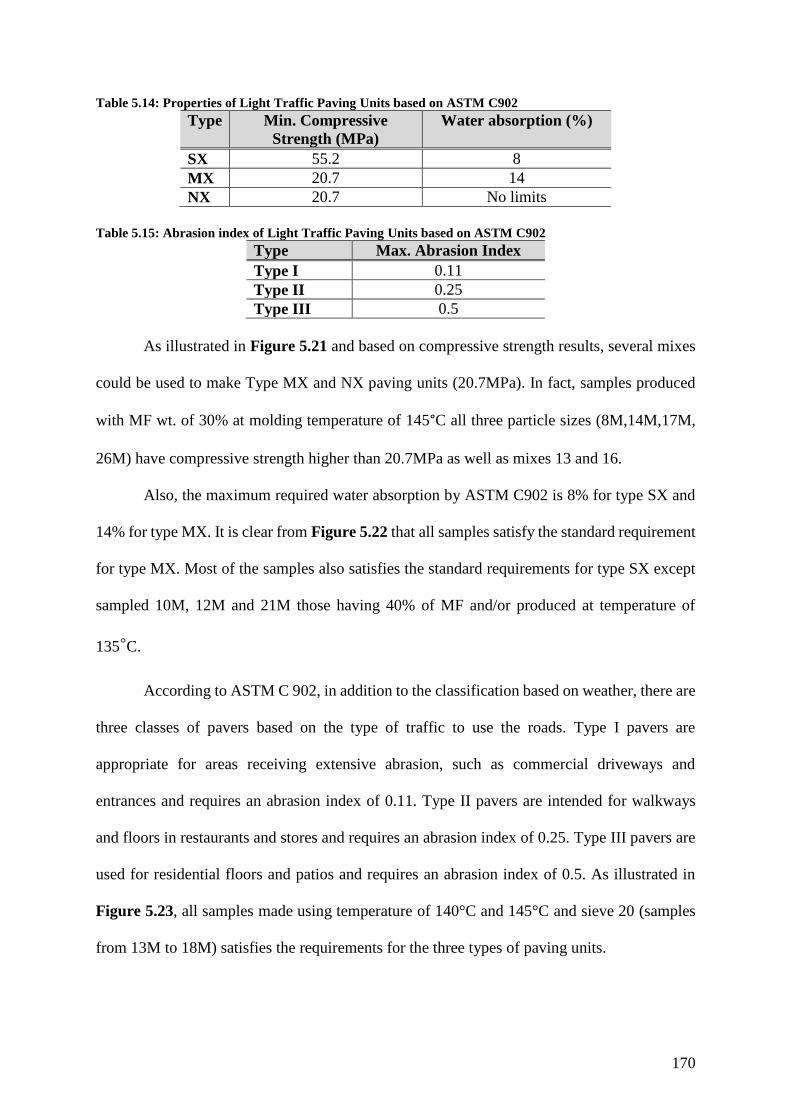
170
Table 5.14: Properties of Light Traffic Paving Units based on ASTM C902
Type Min. Compressive
Strength (MPa)
Water absorption (%)
SX 55.2 8
MX 20.7 14
NX 20.7 No limits
Table 5.15: Abrasion index of Light Traffic Paving Units based on ASTM C902
Type Max. Abrasion Index
Type I 0.11
Type II 0.25
Type III 0.5
As illustrated in Figure 5.21 and based on compressive strength results, several mixes
could be used to make Type MX and NX paving units (20.7MPa). In fact, samples produced
with MF wt. of 30% at molding temperature of 145°C all three particle sizes (8M,14M,17M,
26M) have compressive strength higher than 20.7MPa as well as mixes 13 and 16.
Also, the maximum required water absorption by ASTM C902 is 8% for type SX and
14% for type MX. It is clear from Figure 5.22 that all samples satisfy the standard requirement
for type MX. Most of the samples also satisfies the standard requirements for type SX except
sampled 10M, 12M and 21M those having 40% of MF and/or produced at temperature of
135°C.
According to ASTM C 902, in addition to the classification based on weather, there are
three classes of pavers based on the type of traffic to use the roads. Type I pavers are
appropriate for areas receiving extensive abrasion, such as commercial driveways and
entrances and requires an abrasion index of 0.11. Type II pavers are intended for walkways
and floors in restaurants and stores and requires an abrasion index of 0.25. Type III pavers are
used for residential floors and patios and requires an abrasion index of 0.5. As illustrated in
Figure 5.23, all samples made using temperature of 140°C and 145°C and sieve 20 (samples
from 13M to 18M) satisfies the requirements for the three types of paving units.
171
Hence, from the above discussion it could be concluded that the sample molded at temperature
of 145°C and containing 30 % wt. of sieve 20 MF (17M) could be used to produce MX and
NX types of Light Traffic Paving units with highest mechanical properties.
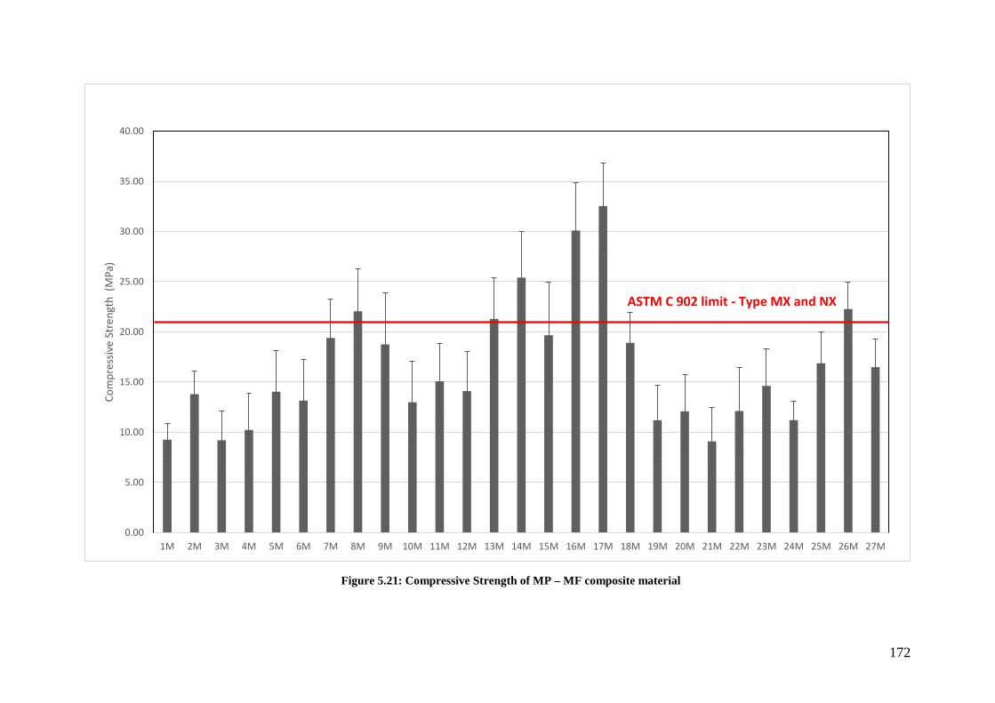
172
Figure 5.21: Compressive Strength of MP – MF composite material
0.00
5.00
10.00
15.00
20.00
25.00
30.00
35.00
40.00
1M 2M 3M 4M 5M 6M 7M 8M 9M 10M 11M 12M 13M 14M 15M 16M 17M 18M 19M 20M 21M 22M 23M 24M 25M 26M 27M
Co
mp
ress
ive
Stre
ngt
h (
MP
a)
ASTM C 902 limit - Type MX and NX
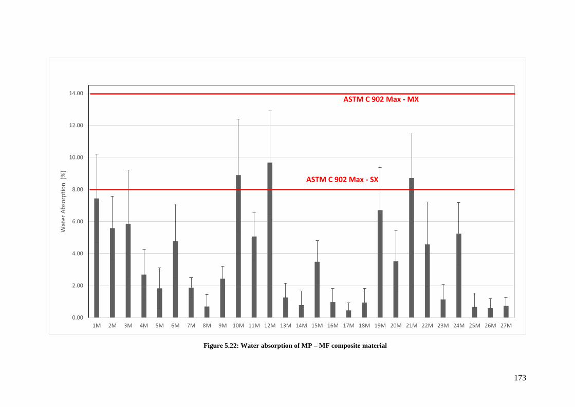
173
Figure 5.22: Water absorption of MP – MF composite material
0.00
2.00
4.00
6.00
8.00
10.00
12.00
14.00
1M 2M 3M 4M 5M 6M 7M 8M 9M 10M 11M 12M 13M 14M 15M 16M 17M 18M 19M 20M 21M 22M 23M 24M 25M 26M 27M
Wat
er A
bso
rpti
on
(%
)
ASTM C 902 Max - SX
ASTM C 902 Max - MX
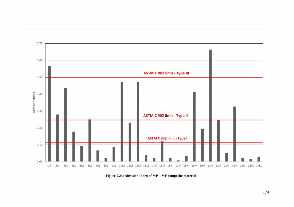
174
Figure 5.23: Abrasion Index of MP – MF composite material
0.00
0.10
0.20
0.30
0.40
0.50
0.60
0.70
1M 2M 3M 4M 5M 6M 7M 8M 9M 10M 11M 12M 13M 14M 15M 16M 17M 18M 19M 20M 21M 22M 23M 24M 25M 26M 27M
Ab
rasi
on
Ind
ex
ASTM C 902 limit - Type II
ASTM C 902 limit - Type III
ASTM C 902 limit - Type I
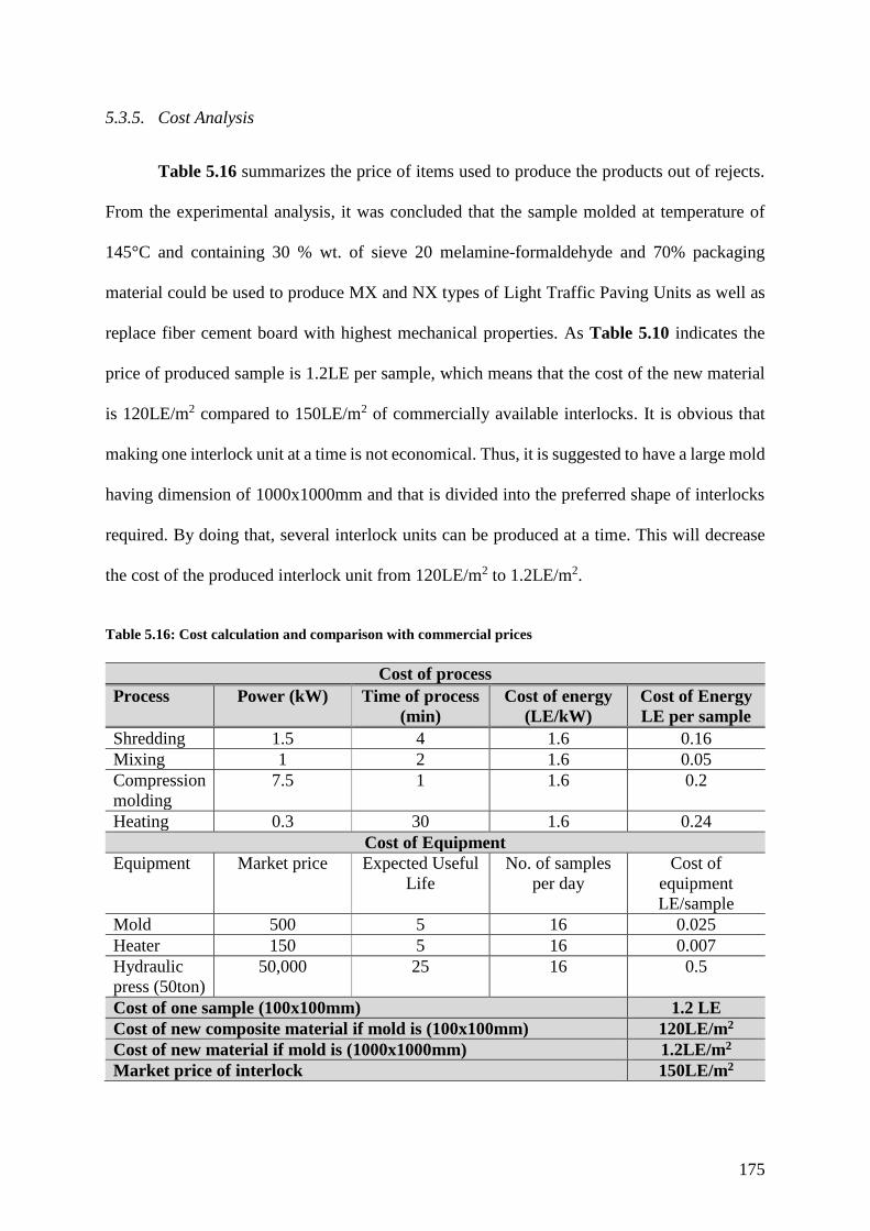
175
5.3.5. Cost Analysis
Table 5.16 summarizes the price of items used to produce the products out of rejects.
From the experimental analysis, it was concluded that the sample molded at temperature of
145°C and containing 30 % wt. of sieve 20 melamine-formaldehyde and 70% packaging
material could be used to produce MX and NX types of Light Traffic Paving Units as well as
replace fiber cement board with highest mechanical properties. As Table 5.10 indicates the
price of produced sample is 1.2LE per sample, which means that the cost of the new material
is 120LE/m2 compared to 150LE/m2 of commercially available interlocks. It is obvious that
making one interlock unit at a time is not economical. Thus, it is suggested to have a large mold
having dimension of 1000x1000mm and that is divided into the preferred shape of interlocks
required. By doing that, several interlock units can be produced at a time. This will decrease
the cost of the produced interlock unit from 120LE/m2 to 1.2LE/m2.
Table 5.16: Cost calculation and comparison with commercial prices
Cost of process
Process Power (kW) Time of process
(min)
Cost of energy
(LE/kW)
Cost of Energy
LE per sample
Shredding 1.5 4 1.6 0.16
Mixing 1 2 1.6 0.05
Compression
molding
7.5 1 1.6 0.2
Heating 0.3 30 1.6 0.24
Cost of Equipment
Equipment Market price Expected Useful
Life
No. of samples
per day
Cost of
equipment
LE/sample
Mold 500 5 16 0.025
Heater 150 5 16 0.007
Hydraulic
press (50ton)
50,000 25 16 0.5
Cost of one sample (100x100mm) 1.2 LE
Cost of new composite material if mold is (100x100mm) 120LE/m2
Cost of new material if mold is (1000x1000mm) 1.2LE/m2
Market price of interlock 150LE/m2
176
5.3.6. Conclusion
Compression molding technique is used to produce the composite material from waste
multi-layer packaging material as the matrix and melamine-formaldehyde as the filling
material. In compression molding, the sample is subject to 50bar pressure and heat for 30min.
The effect of the following three factors are examined: (1) temperature, (2) %wt. of filling
material, and (3) particle size of filling material. Pilot experiments are conducted first to
determine the different levels that will be tested for each factors. The pilot experiments
indicated that good samples are obtained using volume fraction ranging from 20% to 40% of
filling material, heating temperature ranging from 135 to 145℃, and particle size ranging from
sieve 16 to sieve 40. Three levels for each factor are determined and a full design of experiment
is conducted. Hence, 27 combinations are tested, and each combination is replicated 3 times.
For higher accuracy samples are produced at random order using Design Expert software. The
following tests are conducted on all 81 samples: compressive strength, moisture absorption,
abrasion resistance, flexural strength and density. Also, abrasion index of all samples is
calculated from water absorption and compressive strength values. Finally, leachate test is
conducted to make sure that the produced material can be safely used without adverse effect
on the environment.
The experimental results indicated that compression molding temperature has the
highest significant effect on the compressive and flexural strength of the samples. The results
reveal that highest compressive and flexural strength are achieved by increasing the
temperature during compression molding. This is attributed to the fact that highest temperature
allows the packaging material to melt more; therefore, packaging material wet the filling
material more leading to better adhesion between the matrix and filling material. The results
show that the compressive strength as well as the flexural strength can be described by a
quadratic model expressed as a function of compression molding temperature (°C), MF %wt.,
177
and MF particle size (µm). Also, the results reveal that all samples have low densities, low
water absorption properties and high abrasion resistance.
The experimental results indicate that the highest mechanical properties are obtained in
samples produced using molding temperature of 145°C, melamine-formaldehyde having a
particle size of sieve 20 and 30%wt. fraction of melamine-formaldehyde. In fact, the produced
material is found to have compressive strength of 32.54MPa, flexural strength of 18.42MPa,
water absorption of 0.32%, density of 0.97g/cm3 and abrasion index of 0.01. The resulting
product is found to be competitive to commercial MX and NX types of Light Traffic Paving
Units in terms of cost and mechanical performance. In fact, the cost of produced material is
1.2LE/m2 compared to 150LE/m2 for interlock market price.
Also, substituting melamine-formaldehyde with other filling material like EPDM rubber waste
or sand and substituting the packaging material with plastic bags waste showed to produce
material slightly lower mechanical properties but can still be a competitive substitute to
produce interlocks and substitute cement board.
The application of Waste to Business (W2B) model introduced in chapter 3, in recycling
of rejects to produce marketable products are beneficial for the rural communities not only
from an economic point of view, but also will allow rural areas to convert the piles of
unrecyclable waste – piling up in streets, waterways and dumpsites and causing environmental
and health problem – into paving units that give aesthetic views to rural villages.
5.4. Development of innovative cold technology to produce bricks from
rejects
4.5.1. Methodology
Materials
Four types of waste rejects are used in this experiment:
Contaminated plastic bags waste
178
Melamine-formaldehyde (MF) – Old plates made of MF are collected, cleaned and
crushed into powder
Waste Marble powder (WMP)
Sand
Traditional cement bricks are made of cement, sand, gravel and other fine and coarse
aggregates. Then water is added to activate the cement which is the element responsible for
binding the mix together to form one solid object. Several studies have been conducted to study
the effect of replacing cement or sand with waste material.
Some studies have been conducted to partially replace cement with marble powder or
substitute limestone in cement. During the production of marble studies indicated that 25% of
the original marble mass is lost in the form of powder, which causes many environmental
problems if not disposed of properly.
Sharma et al. [198], studied the effect of partially replacing sand with waste marble powder
and reported that adding waste marble powder with up to 5% by weight of sand increases the
strength properties of the brick. Vigneshpandian et al. [199], studied replacing cement with
waste marble powder with different proportions (25%, 50% and 100%) of the weight of
cement. The study revealed that optimum replacement rate by marble powder to sand in
concrete was 50%. Several other studies have been conducted and showed that marble powder
can be used as a replacement material for cement. These studies revealed that adding 10%
marble powder with cement gives high strength to the material compared to the control
concrete [200].
Very few studies reported the effect of partially replacing cement with waste plastics.
Kumar and Gomathi [201], studied the effect of mixing high-density polyethylene (HDPE) and
polyethylene (PE) plastic bottles and bags with sand, lime, fly ash and gypsum to produce a
brick. The test results showed that the partial replacement of natural sand by crushed waste
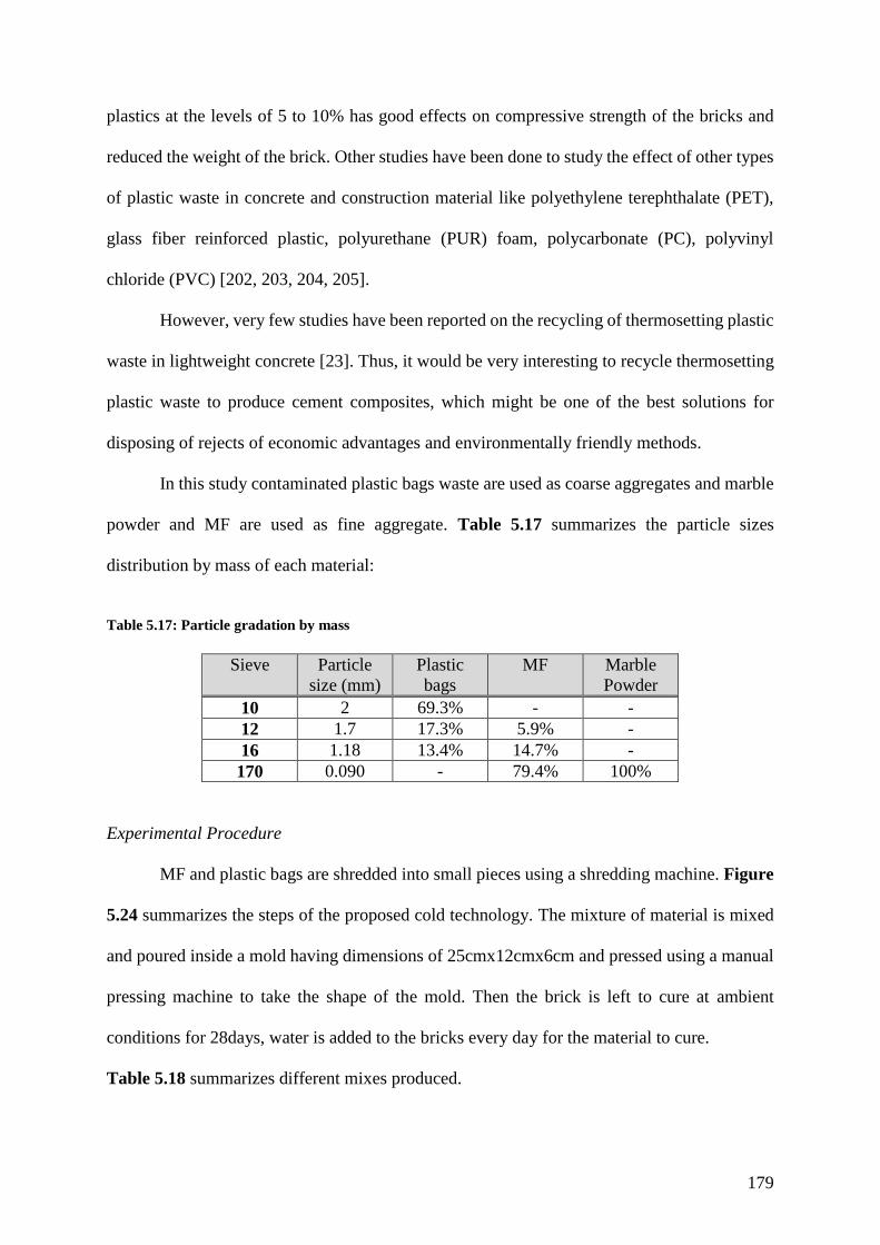
179
plastics at the levels of 5 to 10% has good effects on compressive strength of the bricks and
reduced the weight of the brick. Other studies have been done to study the effect of other types
of plastic waste in concrete and construction material like polyethylene terephthalate (PET),
glass fiber reinforced plastic, polyurethane (PUR) foam, polycarbonate (PC), polyvinyl
chloride (PVC) [202, 203, 204, 205].
However, very few studies have been reported on the recycling of thermosetting plastic
waste in lightweight concrete [23]. Thus, it would be very interesting to recycle thermosetting
plastic waste to produce cement composites, which might be one of the best solutions for
disposing of rejects of economic advantages and environmentally friendly methods.
In this study contaminated plastic bags waste are used as coarse aggregates and marble
powder and MF are used as fine aggregate. Table 5.17 summarizes the particle sizes
distribution by mass of each material:
Table 5.17: Particle gradation by mass
Sieve Particle
size (mm)
Plastic
bags
MF Marble
Powder
10 2 69.3% - -
12 1.7 17.3% 5.9% -
16 1.18 13.4% 14.7% -
170 0.090 - 79.4% 100%
Experimental Procedure
MF and plastic bags are shredded into small pieces using a shredding machine. Figure
5.24 summarizes the steps of the proposed cold technology. The mixture of material is mixed
and poured inside a mold having dimensions of 25cmx12cmx6cm and pressed using a manual
pressing machine to take the shape of the mold. Then the brick is left to cure at ambient
conditions for 28days, water is added to the bricks every day for the material to cure.
Table 5.18 summarizes different mixes produced.

180
Table 5.18: Mixes used in cold technology
Mix No. Cement Plastic
bags
Sand Marble
Powder
MF Cement to
water ratio
M1 25 30 15 25 5 0.5
M2 20 30 15 30 5 0.5
M3 25 30 15 15 15 0.5
M4 20 30 15 20 15 0.5
M5 25 30 15 20 10 0.5
M6 20 30 15 25 10 0.5
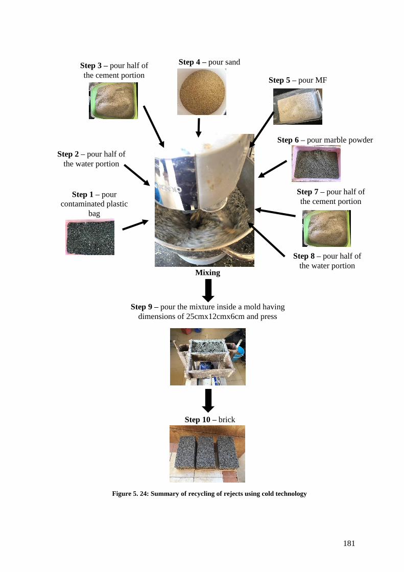
181
Figure 5. 24: Summary of recycling of rejects using cold technology
Step 7 – pour half of
the cement portion
Step 4 – pour sand
Step 6 – pour marble powder
Step 5 – pour MF
Step 3 – pour half of
the cement portion
Step 1 – pour
contaminated plastic
bag
Step 2 – pour half of
the water portion
Step 8 – pour half of
the water portion
Step 9 – pour the mixture inside a mold having
dimensions of 25cmx12cmx6cm and press
Step 10 – brick
Mixing

182
Statistical Analysis
All results were presented as the average of three replicates, and the means among
different treatments were compared using one-way ANOVA using SPPS version 23. The null
hypothesis states that the population means are all equal. A significance level α =0.05 is used.
4.5.2. Measured Properties
Compressive Strength
The compression machine (Figure 5.25) is used to measure the compressive strength
of the bricks. The compressive strength of bricks is measured according to ASTM standard test
method C140 “Sampling and Testing Concrete Masonry Units”. The surface of the sample is
cleaned and leveled, then the sample is placed in the machine and the gate of the machine is
closed. The machine record automatically the load at which the brick fails in kilo Newton (kN).
The compressive strength of the sample is calculated using the following equation:
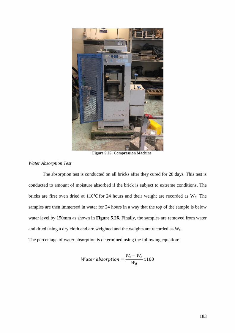
183
Figure 5.25: Compression Machine
Water Absorption Test
The absorption test is conducted on all bricks after they cured for 28 days. This test is
conducted to amount of moisture absorbed if the brick is subject to extreme conditions. The
bricks are first oven dried at 110℃ for 24 hours and their weight are recorded as Wd. The
samples are then immersed in water for 24 hours in a way that the top of the sample is below
water level by 150mm as shown in Figure 5.26. Finally, the samples are removed from water
and dried using a dry cloth and are weighted and the weights are recorded as Ws.
The percentage of water absorption is determined using the following equation:
𝑊𝑎𝑡𝑒𝑟 𝑎𝑏𝑠𝑜𝑟𝑝𝑡𝑖𝑜𝑛 =𝑊𝑠 − 𝑊𝑑
𝑊𝑑𝑥100
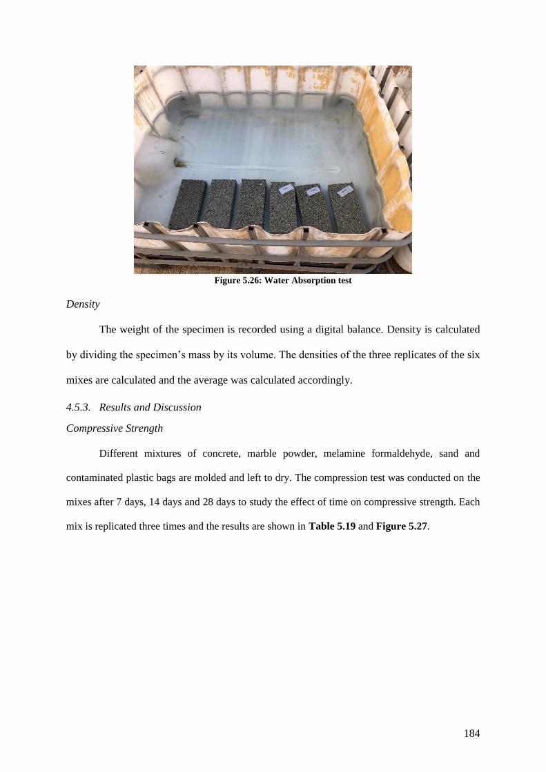
184
Figure 5.26: Water Absorption test
Density
The weight of the specimen is recorded using a digital balance. Density is calculated
by dividing the specimen’s mass by its volume. The densities of the three replicates of the six
mixes are calculated and the average was calculated accordingly.
4.5.3. Results and Discussion
Compressive Strength
Different mixtures of concrete, marble powder, melamine formaldehyde, sand and
contaminated plastic bags are molded and left to dry. The compression test was conducted on the
mixes after 7 days, 14 days and 28 days to study the effect of time on compressive strength. Each
mix is replicated three times and the results are shown in Table 5.19 and Figure 5.27.
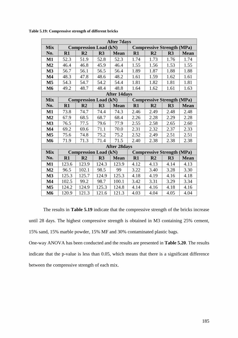
185
Table 5.19: Compressive strength of different bricks
After 7days
Mix
No.
Compression Load (kN) Compressive Strength (MPa)
R1 R2 R3 Mean R1 R2 R3 Mean
M1 52.3 51.9 52.8 52.3 1.74 1.73 1.76 1.74
M2 46.4 46.8 45.9 46.4 1.55 1.56 1.53 1.55
M3 56.7 56.1 56.5 56.4 1.89 1.87 1.88 1.88
M4 48.3 47.8 48.6 48.2 1.61 1.59 1.62 1.61
M5 54.3 54.7 54.2 54.4 1.81 1.82 1.81 1.81
M6 49.2 48.7 48.4 48.8 1.64 1.62 1.61 1.63
After 14days
Mix
No.
Compression Load (kN) Compressive Strength (MPa)
R1 R2 R3 Mean R1 R2 R3 Mean
M1 73.8 74.7 74.4 74.3 2.46 2.49 2.48 2.48
M2 67.9 68.5 68.7 68.4 2.26 2.28 2.29 2.28
M3 76.5 77.5 79.6 77.9 2.55 2.58 2.65 2.60
M4 69.2 69.6 71.1 70.0 2.31 2.32 2.37 2.33
M5 75.6 74.8 75.2 75.2 2.52 2.49 2.51 2.51
M6 71.9 71.3 71.4 71.5 2.40 2.38 2.38 2.38
After 28days
Mix
No.
Compression Load (kN) Compressive Strength (MPa)
R1 R2 R3 Mean R1 R2 R3 Mean
M1 123.6 123.9 124.3 123.9 4.12 4.13 4.14 4.13
M2 96.5 102.1 98.5 99 3.22 3.40 3.28 3.30
M3 125.3 125.7 124.9 125.3 4.18 4.19 4.16 4.18
M4 102.5 99.2 98.7 100.1 3.42 3.31 3.29 3.34
M5 124.2 124.9 125.3 124.8 4.14 4.16 4.18 4.16
M6 120.9 121.3 121.6 121.3 4.03 4.04 4.05 4.04
The results in Table 5.19 indicate that the compressive strength of the bricks increase
until 28 days. The highest compressive strength is obtained in M3 containing 25% cement,
15% sand, 15% marble powder, 15% MF and 30% contaminated plastic bags.
One-way ANOVA has been conducted and the results are presented in Table 5.20. The results
indicate that the p-value is less than 0.05, which means that there is a significant difference
between the compressive strength of each mix.
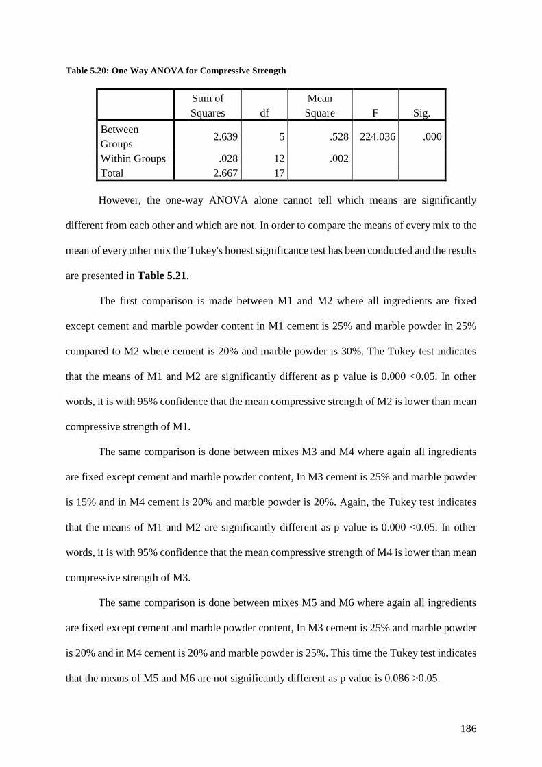
186
Table 5.20: One Way ANOVA for Compressive Strength
Sum of
Squares df
Mean
Square F Sig.
Between
Groups 2.639 5 .528 224.036 .000
Within Groups .028 12 .002
Total 2.667 17
However, the one-way ANOVA alone cannot tell which means are significantly
different from each other and which are not. In order to compare the means of every mix to the
mean of every other mix the Tukey's honest significance test has been conducted and the results
are presented in Table 5.21.
The first comparison is made between M1 and M2 where all ingredients are fixed
except cement and marble powder content in M1 cement is 25% and marble powder in 25%
compared to M2 where cement is 20% and marble powder is 30%. The Tukey test indicates
that the means of M1 and M2 are significantly different as p value is 0.000 <0.05. In other
words, it is with 95% confidence that the mean compressive strength of M2 is lower than mean
compressive strength of M1.
The same comparison is done between mixes M3 and M4 where again all ingredients
are fixed except cement and marble powder content, In M3 cement is 25% and marble powder
is 15% and in M4 cement is 20% and marble powder is 20%. Again, the Tukey test indicates
that the means of M1 and M2 are significantly different as p value is 0.000 <0.05. In other
words, it is with 95% confidence that the mean compressive strength of M4 is lower than mean
compressive strength of M3.
The same comparison is done between mixes M5 and M6 where again all ingredients
are fixed except cement and marble powder content, In M3 cement is 25% and marble powder
is 20% and in M4 cement is 20% and marble powder is 25%. This time the Tukey test indicates
that the means of M5 and M6 are not significantly different as p value is 0.086 >0.05.
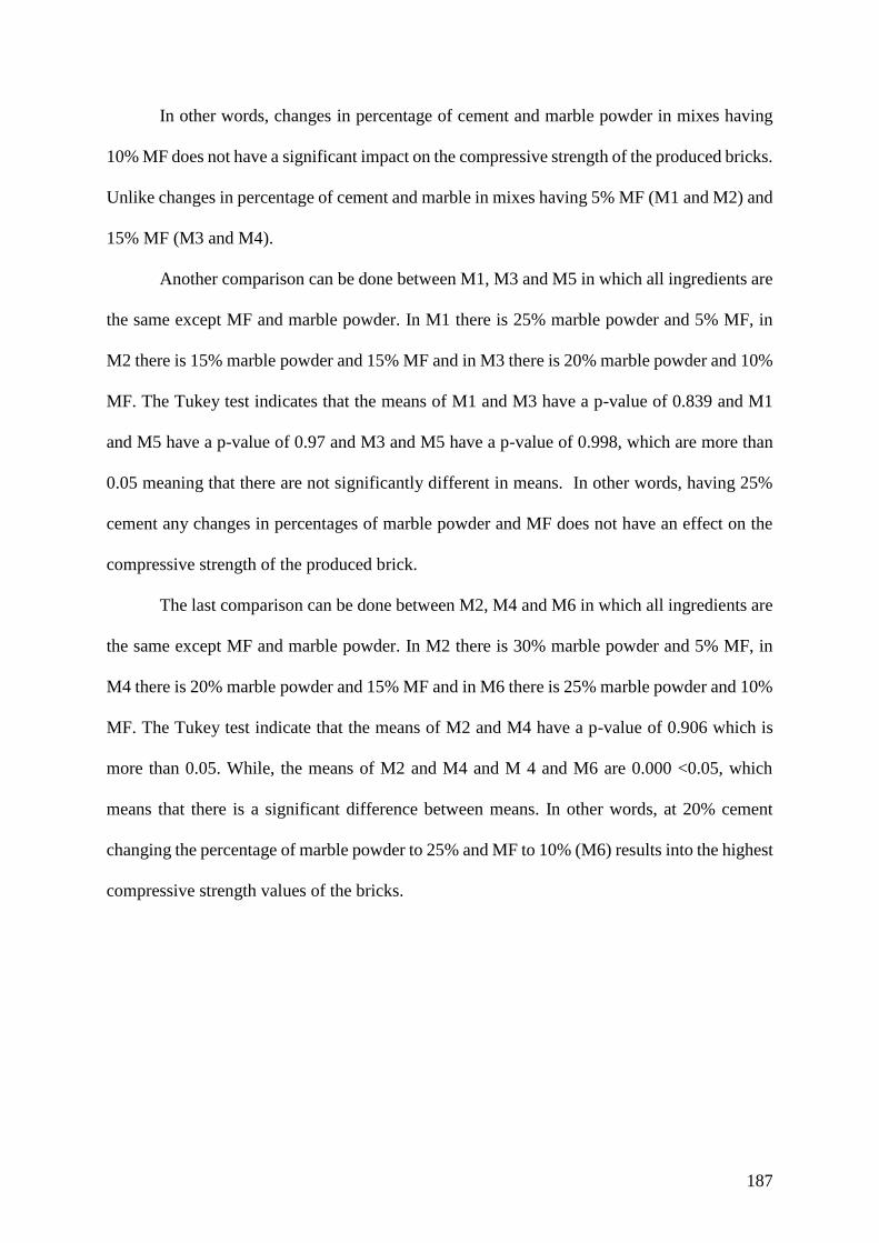
187
In other words, changes in percentage of cement and marble powder in mixes having
10% MF does not have a significant impact on the compressive strength of the produced bricks.
Unlike changes in percentage of cement and marble in mixes having 5% MF (M1 and M2) and
15% MF (M3 and M4).
Another comparison can be done between M1, M3 and M5 in which all ingredients are
the same except MF and marble powder. In M1 there is 25% marble powder and 5% MF, in
M2 there is 15% marble powder and 15% MF and in M3 there is 20% marble powder and 10%
MF. The Tukey test indicates that the means of M1 and M3 have a p-value of 0.839 and M1
and M5 have a p-value of 0.97 and M3 and M5 have a p-value of 0.998, which are more than
0.05 meaning that there are not significantly different in means. In other words, having 25%
cement any changes in percentages of marble powder and MF does not have an effect on the
compressive strength of the produced brick.
The last comparison can be done between M2, M4 and M6 in which all ingredients are
the same except MF and marble powder. In M2 there is 30% marble powder and 5% MF, in
M4 there is 20% marble powder and 15% MF and in M6 there is 25% marble powder and 10%
MF. The Tukey test indicate that the means of M2 and M4 have a p-value of 0.906 which is
more than 0.05. While, the means of M2 and M4 and M 4 and M6 are 0.000 <0.05, which
means that there is a significant difference between means. In other words, at 20% cement
changing the percentage of marble powder to 25% and MF to 10% (M6) results into the highest
compressive strength values of the bricks.

188
Table 5.21: Tukey’s HSD test for Compressive Strength
(I)
Mix
(J)
Mix
Mean
Difference
(I-J)
Std.
Error Sig.
95% Confidence Interval
Lower
Bound
Upper
Bound
M1 M2 .83000* .03963 .000 .6969 .9631
M3 -.04667 .03963 .839 -.1798 .0864
M4 .79000* .03963 .000 .6569 .9231
M5 -.03000 .03963 .970 -.1631 .1031
M6 .09000 .03963 .276 -.0431 .2231
M2 M1 -.83000* .03963 .000 -.9631 -.6969
M3 -.87667* .03963 .000 -1.0098 -.7436
M4 -.04000 .03963 .906 -.1731 .0931
M5 -.86000* .03963 .000 -.9931 -.7269
M6 -.74000* .03963 .000 -.8731 -.6069
M3 M1 .04667 .03963 .839 -.0864 .1798
M2 .87667* .03963 .000 .7436 1.0098
M4 .83667* .03963 .000 .7036 .9698
M5 .01667 .03963 .998 -.1164 .1498
M6 .13667* .03963 .043 .0036 .2698
M4 M1 -.79000* .03963 .000 -.9231 -.6569
M2 .04000 .03963 .906 -.0931 .1731
M3 -.83667* .03963 .000 -.9698 -.7036
M5 -.82000* .03963 .000 -.9531 -.6869
M6 -.70000* .03963 .000 -.8331 -.5669
M5 M1 .03000 .03963 .970 -.1031 .1631
M2 .86000* .03963 .000 .7269 .9931
M3 -.01667 .03963 .998 -.1498 .1164
M4 .82000* .03963 .000 .6869 .9531
M6 .12000 .03963 .086 -.0131 .2531
M6 M1 -.09000 .03963 .276 -.2231 .0431
M2 .74000* .03963 .000 .6069 .8731
M3 -.13667* .03963 .043 -.2698 -.0036
M4 .70000* .03963 .000 .5669 .8331
M5 -.12000 .03963 .086 -.2531 .0131
The compressive strength of the produced bricks is compared against the compressive
strength required by ASTM C129-17 for non-load bearing concrete Masonry Units and the
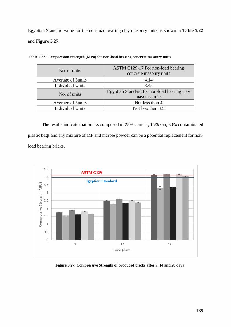
189
Egyptian Standard value for the non-load bearing clay masonry units as shown in Table 5.22
and Figure 5.27.
Table 5.22: Compression Strength (MPa) for non-load bearing concrete masonry units
No. of units ASTM C129-17 For non-load bearing
concrete masonry units
Average of 3units 4.14
Individual Units 3.45
No. of units Egyptian Standard for non-load bearing clay
masonry units
Average of 5units Not less than 4
Individual Units Not less than 3.5
The results indicate that bricks composed of 25% cement, 15% san, 30% contaminated
plastic bags and any mixture of MF and marble powder can be a potential replacement for non-
load bearing bricks.
Figure 5.27: Compressive Strength of produced bricks after 7, 14 and 28 days
0
0.5
1
1.5
2
2.5
3
3.5
4
4.5
7 14 28
Co
mp
ress
ive
Stre
ngt
h (
MP
a)
Time (days)
ASTM C129
Egyptian Standard
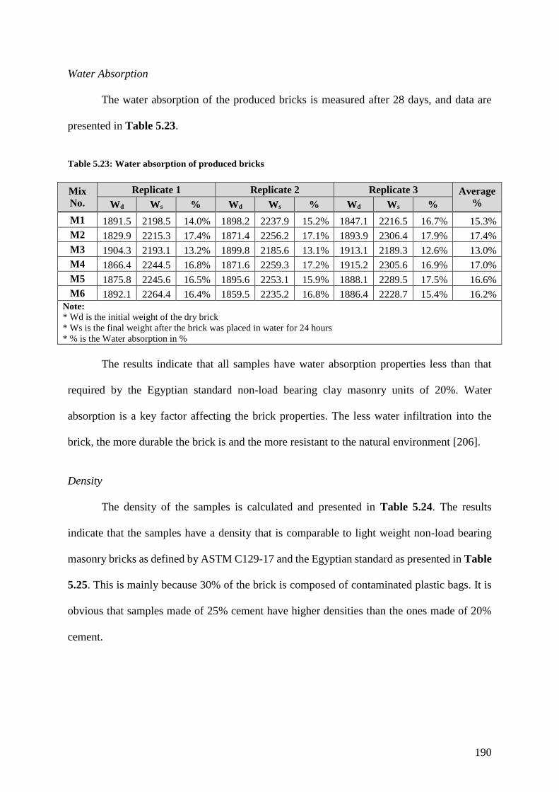
190
Water Absorption
The water absorption of the produced bricks is measured after 28 days, and data are
presented in Table 5.23.
Table 5.23: Water absorption of produced bricks
Mix
No.
Replicate 1 Replicate 2 Replicate 3 Average
% Wd Ws % Wd Ws % Wd Ws %
M1 1891.5 2198.5 14.0% 1898.2 2237.9 15.2% 1847.1 2216.5 16.7% 15.3%
M2 1829.9 2215.3 17.4% 1871.4 2256.2 17.1% 1893.9 2306.4 17.9% 17.4%
M3 1904.3 2193.1 13.2% 1899.8 2185.6 13.1% 1913.1 2189.3 12.6% 13.0%
M4 1866.4 2244.5 16.8% 1871.6 2259.3 17.2% 1915.2 2305.6 16.9% 17.0%
M5 1875.8 2245.6 16.5% 1895.6 2253.1 15.9% 1888.1 2289.5 17.5% 16.6%
M6 1892.1 2264.4 16.4% 1859.5 2235.2 16.8% 1886.4 2228.7 15.4% 16.2% Note: * Wd is the initial weight of the dry brick
* Ws is the final weight after the brick was placed in water for 24 hours
* % is the Water absorption in %
The results indicate that all samples have water absorption properties less than that
required by the Egyptian standard non-load bearing clay masonry units of 20%. Water
absorption is a key factor affecting the brick properties. The less water infiltration into the
brick, the more durable the brick is and the more resistant to the natural environment [206].
Density
The density of the samples is calculated and presented in Table 5.24. The results
indicate that the samples have a density that is comparable to light weight non-load bearing
masonry bricks as defined by ASTM C129-17 and the Egyptian standard as presented in Table
5.25. This is mainly because 30% of the brick is composed of contaminated plastic bags. It is
obvious that samples made of 25% cement have higher densities than the ones made of 20%
cement.
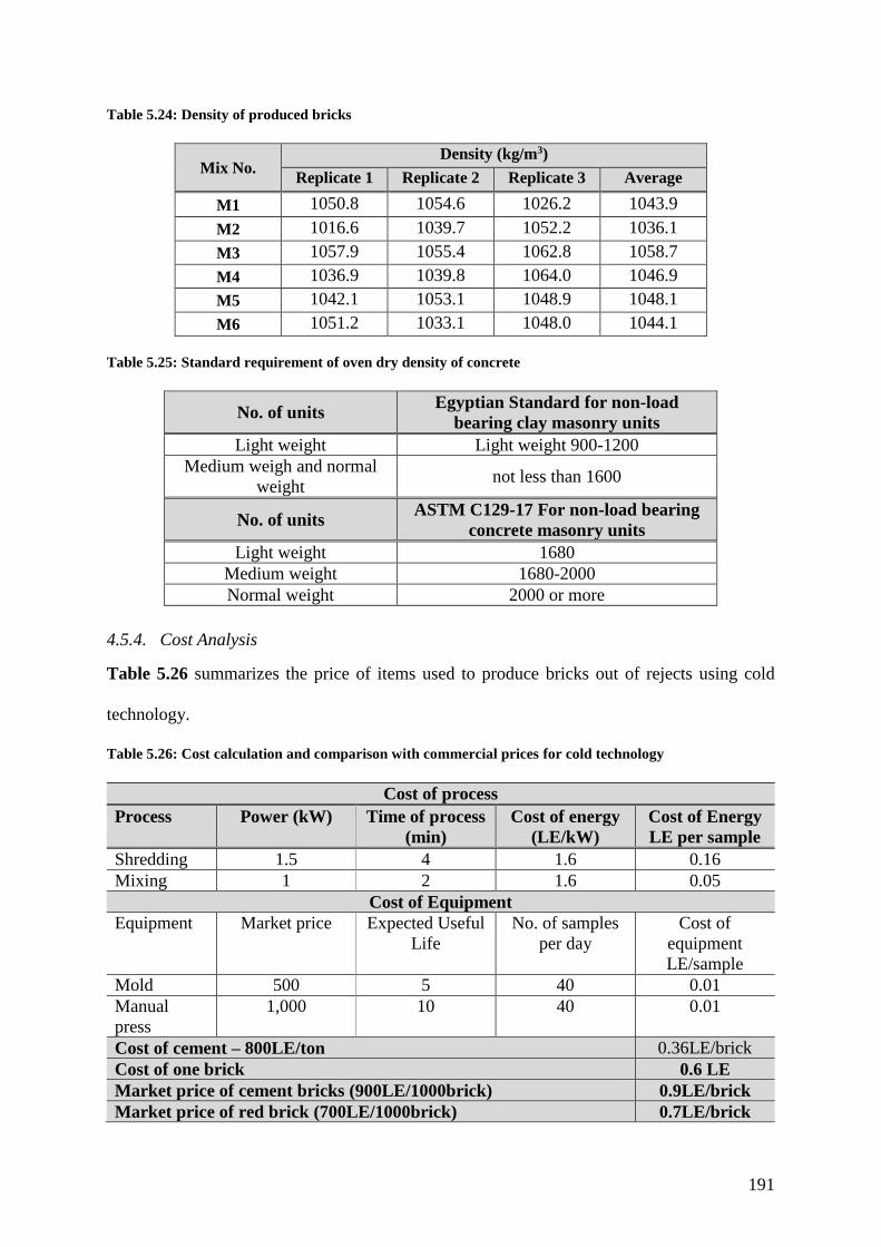
191
Table 5.24: Density of produced bricks
Mix No. Density (kg/m3)
Replicate 1 Replicate 2 Replicate 3 Average
M1 1050.8 1054.6 1026.2 1043.9
M2 1016.6 1039.7 1052.2 1036.1
M3 1057.9 1055.4 1062.8 1058.7
M4 1036.9 1039.8 1064.0 1046.9
M5 1042.1 1053.1 1048.9 1048.1
M6 1051.2 1033.1 1048.0 1044.1
Table 5.25: Standard requirement of oven dry density of concrete
No. of units Egyptian Standard for non-load
bearing clay masonry units
Light weight Light weight 900-1200
Medium weigh and normal
weight not less than 1600
No. of units ASTM C129-17 For non-load bearing
concrete masonry units
Light weight 1680
Medium weight 1680-2000
Normal weight 2000 or more
4.5.4. Cost Analysis
Table 5.26 summarizes the price of items used to produce bricks out of rejects using cold
technology.
Table 5.26: Cost calculation and comparison with commercial prices for cold technology
Cost of process
Process Power (kW) Time of process
(min)
Cost of energy
(LE/kW)
Cost of Energy
LE per sample
Shredding 1.5 4 1.6 0.16
Mixing 1 2 1.6 0.05
Cost of Equipment
Equipment Market price Expected Useful
Life
No. of samples
per day
Cost of
equipment
LE/sample
Mold 500 5 40 0.01
Manual
press
1,000 10 40 0.01
Cost of cement – 800LE/ton 0.36LE/brick
Cost of one brick 0.6 LE
Market price of cement bricks (900LE/1000brick) 0.9LE/brick
Market price of red brick (700LE/1000brick) 0.7LE/brick
192
It is worth mentioning that all calculations are based on cost of raw materials only
excluding transportation and labor wages. Also, the costs of landfilling, conservation of natural
resources and environmental impact of dumping rejects in streets and waterways are not
included.
4.5.5. Conclusion
In this section an innovative technique is proposed to produce bricks from waste rejects
with minimal energy cost. This technique consists mixing contaminated plastic bags as coarse
aggregates with sand, marble powder and melamine-formaldehyde as fine aggregates with
cement. The mix is then pressed using a manual pressing machine without applying heat for
few minutes to take the shape of the mold. Then the brick is left to cure at ambient conditions
and water is added every day.
The experimental results indicated that the highest properties is obtained after 28days
of curing in the mix made of 25%cement, 30% contaminated plastic bags, 15%sand, 15%
marble powder, 15% melamine-formaldehyde. The produced brick is found to have a
compressive strength of 4.18MPa and a water absorption of 13%. The density of the sample is
found to be 1058.7kg/m3, which is considered light weight brick. The resulting product is
found to be competitive to the commercial non-load bearing masonry brick in terms of
mechanical performance and cost. In fact, the cost of produced material is 0.6LE/brick
compared to 0.9 LE/brick for cement brick.
The application of Waste to Business (W2B) model introduced in chapter 3 , in recycling of
rejects to produce marketable products are beneficial for the rural communities not only from
an economic point of view, but also will allow rural areas to convert the piles of unrecyclable
waste – piling up in streets, waterways and dumpsites and causing environmental and health
problem – into cement bricks that give aesthetic views to houses and buildings of rural villages.
193
5.5. Conclusion
In this chapter two methods have been proposed to recycle rejects: (1) hot technology and (2)
cold technology. By using the hot technology, a new composite material is produced from
rejects and can be used to produce Light Traffic interlock paving units. Also, the cold
technology can be used to produce material that can be used to produce non-load bearing
masonry brick. In other words, these proposed technologies can be used to produce competitive
products in terms of mechanical properties and cost from rejects.
In addition to the economic benefit, the production of new material from rejects will also have
positive social and environmental impact as follows:
Reduce the amount of rejects and garbage in streets and waterways and thus reduce
health hazard associated with it.
Create new types of job opportunities
Gives the micro-entrepreneurial opportunity to residents of rural areas
Help residents of rural communities have aesthetic spaces by removing the unrecycled
materials from streets and replacing them with cheap interlocks paving units and
masonry bricks for buildings. This will also help protect rural landscape, protect air and
water quality as well as create touristic attractions that can be beneficial for the
economy of the rural areas as well as the economy of the country as a whole.
194
CHAPTER 6– CONCLUSION AND RECOMMENDATIONS
Rural communities in Egypt are confronted with many environmental issues due to the
huge amount of waste generated every year including municipal solid waste (such as metals,
glass, plastics, rejects, ...), wastewater, organic waste (such as agricultural waste and animal
manure, ...) etc. These wastes are poorly disposed of and managed causing serious problems
and burden to the country. These problems cause environmental, ecological, economic and
health pressures. The tragic situation facing rural villages in developing countries cannot be
ignored anymore.
The main goal of this research work is to develop and propose a concept to help rural
communities in Egypt approach full utilization of all types of wastes generated. This research
is divided into three parts. In the first part the concept of Waste to Business (W2B) model is
proposed to help rural communities approach full utilization of their waste. Then, the second
part of this research focuses on recycling of organic waste and rice straw is taken as a case
study. The third part focuses on recycling of municipal solid waste and reject is taken as a case
study.
6.1. Conclusions
6.1.1. Waste to business Model for Sustainable Rural Communities
The object of the first part of this research work is to develop a concept to help rural
communities in Egypt approach full utilization of their different waste streams. In order to
achieve this object, desk research method is used in which secondary data are collected from
different sources including books, journal papers, conference papers, governmental reports,
international organizations’ statistics and websites. In order to gather relevant information to
the problem, some research questions are developed from which a list of key words is
generated. These key words are then used to search for relevant sources. The main limitation

195
encountered during the research is the absence of accurate data regarding the exact amounts
and types of waste generated in rural areas. Most of the published studies focus on waste
management in Great Cairo and very few studies are conducted in rural areas. This lack of data
makes it difficult to estimate numbers such as uncollected waste by geographical location and
the exact amount of waste generated by types.
After thorough study of the gathered literature, the collected data are discussed to reply to the
above questions. Then the limitations of the disposal methods and recycling techniques for
rural villages are identified and the concept of W2B is developed and proposed to help rural
areas in Egypt reach Sustainable Rural Communities.
It is proposed that the government, the rural community, business community and
academic institutions and research centers collaborate to implement W2B model in rural
communities. The W2B model consists of having a facility in each rural community that groups
simple and obtainable technologies. This facility will receive all types of wastes generated in
rural areas, which will be sorted manually and distributed among different units to fully utilize
all types of wastes generated in rural village and produce useful products. Wastewater is stored
in a tank and then used to produce biogas. The slurry from the biogas digester along with
agricultural waste, food waste and animal manure are used in composting process to produce
high quality fertilizer. Yet research is still needed to understand the effect of different additives
on the composting process and to accelerate the process. MSW is then sorted manually and
distributed among different units to produce useful goods depending on the market need of the
village. One type of MSW is reject, material that are hard to recycle, still research is needed to
fully utilize rejects to produce useful good at an affordable manner. Consequently, this facility
will collect all type of wastes generated in the rural village and will recycle them to produce
useful products. By applying this approach, the village will be able to conserve natural
resources, reduce the environmental, health, economic and social problems facing these remote
196
areas due to burning and dumping waste. It will also help in creating new job opportunities and
reduce the cost of goods.
While reviewing different waste streams it became obvious that there are two main
important problems in rural villages in Egypt that need to be studied in depth: (1) recycling of
organic waste, and (2) Recycling or rejects
6.1.2. Sustainable bio-conversion of agricultural waste into high quality organic fertilizer:
case study of rice straw
One of the utmost important problems facing rural villages in Egypt is the huge amount
of organic waste generated every year that are estimated to be 133million tons/year. There are
several types of organic waste and this research focuses on agricultural waste as a type of
organic waste. Egypt generates up to 30 million ton/year of agricultural waste, from which
52% are directly burnt in the fields. One of the main types of agricultural waste generated in
Egypt is rice straw, it is estimated that today around 2.5million tons of rice straw are generated
per year.
Composting is one of the useful methods that can convert large amounts of agricultural
waste into a valuable product that can be used as a source amendement to improve soil
structure, increase its organic matter, and enhance plant growth. However, this method is not
widely practiced in developing countries because it is time consuming and quality of product
received can be unstable. Some studies showed that the use of additives is a beneficial option
to improve nutritional value of compost and accelerate the degradation process. Some of these
amendments include biochar, effective micro-organisms (EM), cellulose decomposing
bacteria, starters containing bacillus, fungi, yeast, lactic acid bacteria, and animal manure.
Several producers of these additives claim that they can generate higher quality compost during
short period of time. Yet, the effect of these additives on the composting process is not fully
studied and understood. The aim of these experiments is to evaluate the effect of different
197
additives on the quality of rice straw compost and to produce high quality soil amendments
and organic fertilizers by composting of rice straw. This part is divided into two sets of
experiments as follows:
The objective of the first set of experiment is to transform rice straw into soil
amendment and evaluate the effect of different additives on the produced compost. In the first
set of experiment rice straw is inoculated with animal manure, Chinese starter, cellulose
decomposer and starter from the Egyptian Ministry of agriculture. The results of the first set
of experiments revealed that the application of different additives in composting of rice straw
exhibited an improvement of compost quality. The results of the first set of experiments
revealed a higher decomposition rate of treatment having animal manure, compared to other
treatments. All analysis of the properties of the final compost products containing animal
manure indicated that it was in the range of the matured level after 60 days and can be used
without any limitation
Therefore, a second set of experiment has been conducted with substrate rice straw,
animal manure and mixture of natural rocks inoculated with different types of additives
(including (effective micro-organisms, biochar and Chinese starter) to produce high quality
organic fertilizer. The results revealed that the application of different additives in composting
of rice straw exhibit an improvement in maturation time and final product quality. In fact, all
piles reached maturation after around 42 days. All analysis of the properties of the final
products indicated that it was in the range of the matured level and can be used without any
limitation as an organic fertilizer. The highest decomposition rate and highest organic fertilizer
quality was obtained in pile containing rice straw and 40% of animal manure mixed with
natural rocks (2.5% of rock phosphate, 2.5% feldspar, 2.5% sulfur, 2.5% dolomite and 10%
bentonite) and inoculated with 2% of EM and 10% biochar compared to other treatments. Also,
the results showed that adding 20% biochar decreased the quality of the final compost

198
compared to adding 10%. The cost of the produced high-quality organic fertilizer is estimated
to be 330LE/ton, given that each farmer will use the organic waste generated from his land and
will not need extra labor to produce the organic fertilizer compared to chemical fertilizer
market price of 1,700LE/ton to 12,000LE/ton (non-subsidized price). In addition to the direct
cost, the use of chemical fertilizer damages the atmosphere and the water. This damage has an
unforeseen high cost. Therefore, organic fertilizer produced from organic waste can substitute
expensive chemical fertilizer. In addition to economic benefits, reducing the use of chemical
fertilizer will lead to the creation of new job opportunities in rural villages, reduction of soil,
water and air pollution as farmers will sell their waste instead of burning it in the field. Also,
application of organic fertilizer will re-establish the soil structure on the long run.
6.1.3. Approaching full utilization of Municipal Solid Waste: case study of rejects
Another major problems facing rural communities in Egypt is poor municipal solid
waste (MSW) management, which contribute to the health, ecological and environmental
problems facing rural communities. Egypt generates around 21million tons of MSW per year.
More than 35% of waste is either burnt or end up in open, public and random dumpsite causing
many environmental and health problem to rural villages in Egypt. A large part of MSW is
made out of unrecyclable waste known as rejects. There are many types of rejects and this
research focuses on the following types of rejects: (1) packaging materials, (2) thermosets, and
(3) contaminated plastic bags.
The main aim of this part is to propose solution to close the loop for rejects from municipal
solid waste and approach full utilization of rejects.
This part of the research work proposes two techniques to recycle rejects: (1) hot
technology and (2) a cold technology.
In the hot technology compression molding technique is used to produce the composite
material from waste multi-layer packaging material as the matrix and melamine-formaldehyde
as the filling material. In compression molding, the sample is subject to 50bar pressure and
199
heat for 30min. The effect of the following three factors are examined: (1) temperature, (2)
%wt. of filling material, and (3) particle size of filling material. Pilot experiments are
conducted first to determine the different levels that will be tested for each factors. The pilot
experiments indicated that good samples are obtained using volume fraction ranging from 20%
to 40% of filling material, heating temperature ranging from 135 to 145℃, and particle size
ranging from sieve 16 to sieve 40. Three levels for each factor are determined and a full design
of experiment is conducted. Hence, 27 combinations are tested, and each combination is
replicated 3 times. For higher accuracy samples are produced at random order using Design
Expert software. The following tests are conducted on all 81 samples: compressive strength,
moisture absorption, abrasion resistance, flexural strength and density. Also, abrasion index of
all samples is calculated from water absorption and compressive strength values. Finally,
leachate test is conducted to make sure that the produced material can be safely used without
adverse effect on the environment.
The experimental results indicated that compression molding temperature has the
highest significant effect on the compressive and flexural strength of the samples. The results
reveal that highest compressive and flexural strength are achieved by increasing the
temperature during compression molding. This is attributed to the fact that highest temperature
allows the packaging material to melt more; therefore, packaging material wet the filling
material more leading to better adhesion between the matrix and filling material. The results
show that the compressive strength as well as the flexural strength can be described by a
quadratic model expressed as a function of compression molding temperature (°C), MF %wt.,
and MF particle size (µm). Also, the results reveal that all samples have low densities, low
water absorption properties and high abrasion resistance.
The experimental results indicate that the highest mechanical properties are obtained in
samples produced using molding temperature of 145°C, melamine-formaldehyde having a
200
particle size of sieve 20 and 30%wt. fraction of melamine-formaldehyde. In fact, the produced
material is found to have compressive strength of 32.54MPa, flexural strength of 18.42MPa,
water absorption of 0.32%, density of 0.97g/cm3 and abrasion index of 0.01. The resulting
product is found to be competitive to commercial MX and NX types of Light Traffic interlock
paving units in terms of cost and mechanical performance. In fact, the cost of produced material
is 1.2LE/m2 compared to 150LE/m2 for interlock market price.
Also, substituting melamine-formaldehyde with other filling material like EPDM
rubber waste or sand and substituting the packaging material with plastic bags waste showed
to produce material slightly lower mechanical properties but can still be a competitive
substitute to produce interlocks and substitute cement board.
Recycling of rejects are beneficial for the rural communities not only from an economic
point of view, but also will allow rural areas to convert the piles of unrecyclable waste – piling
up in streets, waterways and dumpsites and causing environmental and health problem – into
interlocks that give aesthetic views to rural villages.
In the second part, an innovative cold technology is proposed to produce cement bricks
from rejects. This technique consists mixing contaminated plastic bags as coarse aggregates
with sand, marble powder and melamine-formaldehyde as fine aggregates with cement. The
mix is then pressed using a manual pressing machine without applying heat for few minutes to
take the shape of the mold. Then the brick is left to cure at ambient conditions and water is
added every day.
The experimental results indicated that the highest properties are obtained after 28days
of curing in the mix made of 25%cement, 30% contaminated plastic bags, 15%sand, 15%
marble powder, 15% melamine-formaldehyde. The produced brick is found to have a
compressive strength of 4.18MPa and a water absorption of 13%. The density of the sample is
found to be 1058.7kg/m3, which is considered light weight brick. The resulting product is found

201
to be competitive to the commercial non-load bearing masonry brick in terms of mechanical
performance and cost. In fact, the cost of produced material is 0.6LE/brick compared to
0.9LE/brick for cement brick.
Recycling of rejects to produce marketable products are beneficial for the rural
communities not only from an economic point of view, but also will allow rural areas to convert
the piles of unrecyclable waste – piling up in streets, waterways and dumpsites and causing
environmental and health problem – into cement bricks that will allow resident of rural areas
build their homes in a more affordable way.
6.1.4. Closing the loop and clearing the path towards sustainable rural communities
The concept of W2B is proposed to help the government, the rural community, business
community and academic institutions and research centers collaborate to help rural
communities approach full utilization of wastes. While studying different waste streams two
gaps were identified: (1) recycling of agricultural waste to produce high quality organic
fertilizer in short period of time, and (2) recycling rejects that are perceived as impossible to
recycle and have no value. By tackling these two problems in this research the W2B model
proposed in chapter 3 can be modified and completed as shown in Figure 6.1.
Applying the concept of W2B can contribute to the Egyptian Sustainable Development
Strategy: Egypt Vision 2030 as well as to 4 of the 17 United Nations Sustainable Development
Goals for 2030 which are:
(1) Good health and well-being as by reducing the amount of waste dumped in streets and
water ways all the health problems associated with pollution will be alleviate allowing
people to live a better life,
(2) Decent work and economic growth as different small and simple technologies are
proposed which will create new job opportunities, give the micro-entrepreneurial
202
opportunity to residents of rural areas and produce useful products that have
economic value and reduce the amount of imported products
(3) Sustainable cities and communities: by having the W2B facility in each rural village,
each village will be able to eliminate waste and produce out it useful products based
on the village needs
(4) Responsible consumption and production: by having this facility resident of rural areas
will start being introduced and familiar with the concept of recycling and will start
learning how to reduce the use of material that are hard to recycle and find innovative
ways to recycle their waste
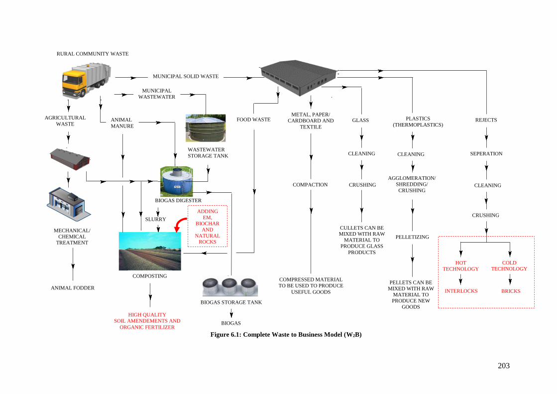
203
Figure 6.1: Complete Waste to Business Model (W2B)
FOOD WASTE REJECTS
SEPERATION
CRUSHING
HOT
TECHNOLOGY
PLASTICS
(THERMOPLASTICS)
CLEANING
AGGLOMERATION/
SHREDDING/
CRUSHING
PELLETIZING
PELLETS CAN BE
MIXED WITH RAW MATERIAL TO
PRODUCE NEW
GOODS
GLASS
CLEANING
CRUSHING
CULLETS CAN BE MIXED WITH RAW
MATERIAL TO
PRODUCE GLASS
PRODUCTS
METAL, PAPER/
CARDBOARD AND
TEXTILE
COMPACTION
COMPRESSED MATERIAL
TO BE USED TO PRODUCE
USEFUL GOODS
RURAL COMMUNITY WASTE
ANIMAL FODDER
MECHANICAL/
CHEMICAL TREATMENT
AGRICULTURAL
WASTE
MUNICIPAL SOLID WASTE
MUNICIPAL
WASTEWATER
WASTEWATER
STORAGE TANK
BIOGAS DIGESTER
SLURRY
BIOGAS STORAGE TANK
BIOGAS
COMPOSTING
HIGH QUALITY
SOIL AMENDEMENTS AND
ORGANIC FERTILIZER
ANIMAL
MANURE
CLEANING
ADDING
EM, BIOCHAR
AND
NATURAL ROCKS
COLD TECHNOLOGY
INTERLOCKS BRICKS

204
6.2. Recommendations
6.2.1. Sustainable bio-conversion of agricultural waste into high quality organic fertilizer:
case study of rice straw
The second part of this research work focuses on recycling of organic waste. One type of
organic waste is agriculture waste. Experimental results indicated that by having additives like
animal manure, biochar, Effective micro-organisms and natural rocks, rice straw can be
transformed into high quality organic fertilizer that meets the Egyptian specifications and can
replace the use of expensive chemical fertilizer. The following are recommendations for future
possible work for this part:
Evaluate the GHG emission from the production of organic fertilizer from waste using
biochar and EM
Evaluate yield from different types of crops (vegetable, fruits, trees) using the
produced organic fertilizer
Develop a mathematical model for the composting process to predict the properties of
organic fertilizer produced and for process optimization
Figure out the optimal addition rate of biochar for successful composting practice
Large scale trial should be done to confirm that the various benefits found from this
pilot- scale study can be repeated in large scale
6.2.2. Approaching full utilization of Municipal Solid Waste: case study of rejects
The third part of the research work focuses on recycling of rejects. Two technologies are
introduced to produce valuable products from rejects: (1) hot technology and (2) cold
technology. The hot technology was shown to be an effective way to produce interlocks from
multi-layer packaging material and melamine-formaldehyde and the cold technology was
proven to be an effective way to produce non-load bearing bricks.
205
The aim of this research was to check the possibility of producing cement bricks using the cold
technology. Based on the literature and the pilot experiments, six mixes were proposed to
produce bricks and were tested. In the future work it is proposed to conduct a full design of
experiment in order to
Identify the effect of different components on the properties of the produced composite
material
Identify the parameter that has the most significant effect on material properties
Develop equations that will allow the prediction of properties for any combination of
parameters
206
REFERENCES
[1] "Egypt in Number". Central Agency for Public Mobilization and Statistics (CAPMAS),
Egypt (2018).
[2] "Income, Expenditure & Consumption Indicators". Central Agency For Public
Mobilization & Statistics (CAPMAS), Egypt (2015).
[3] Elmenofi, G. A., El Bilali, H., Berjan, S., "Governance of Rural Development in Egypt".
Annals of Agricultural Science, vol. 59, no. 2 (2014): 285-296.
[4] Nassar, H., Biltagy. M., "The Nexus of Regional Poverty and Education in Egypt: A
Micro Analysis," International Journal of Economics and Financial Issues, vol. 6, no. 4,
(2016): 1446-1453.
[5] El-Haggar, S., “Sustainable Industrial Design and Waste Management: Cradle-to-Cradle
for Sustainable Development”, Elsevier Academic Press (2007).
[6] El-Haggar S., Omar, H., "Sustainable and Cost-Effective Use of Organic Waste," Current
Trends in Biomedical Engineering & Biosciences, vol. 7, no. 4 (2017).
[7] "Egypt - Country Cooperation Strategy at a Glance," World Health Organization (WHO),
(2018).
[8] USAID, "Global Health - Egypt," 19 April 2018. [Online]. Available:
https://www.usaid.gov/egypt/global-health. [Accessed 3 August 2018].
[9] "Sustainable Development Strategy: Egypt Vision 2030," Minister of Planning,
Monitoring and Administrative Reform (2015).
[10] "Transforming our world: the 2030 Agenda for Sustainable Development," United
Nations (2015).
[11] "Country Report on the Solid Waste Management in Egypt," The Regional Solid Waste
Exchange of Information and Expertise network in Mashreq and Maghreb countries
(2014).
[12] Kamel, S., Abd El-Sattar, H., Vera, D., Jurado, F., "Bioenergy Potential from
Agriculture Residues for Energy Eeneration in Egypt," Renewable and Sustainable
Energy Reviews, vol. 94 (2018): 28-37.
[13] Nakhla, D. A., Hassan, M. G., El-Haggar, S. "Impact of Biomass in Egypt on Climate
Change," Natural Science, vol. 5, no. 6 (2013): 678-684.
[14] Abou Hussein, S. D., Sawan, O. M., "The Utilization of Agricultural Waste as One of
the Environmental Issues in Egypt (A Case Study)," Journal of Applied Sciences
Research, vol. 6, no. 8 (2010): 1116-1124.
[15] Abdel-Rahman, M. A., "Establishment of Efficient Cellulolytic Bacterial Consortium
Potential for Designed Composting of Rice Straw," International Journal of Advanced
Research in Biological Sciences, vol. 3, no. 4 (2016): 211-228.
[16] Abdelhady, S., Borello, D., Shaban, A., Rispoli, F., "Viability Study of Biomass Power
Plant Fired with Rice Straw in Egypt," Energy procedia, vol. 61 (2014): 211-215.
[17] Abdel-Rahman, M. A., Nour El-Din, M., Refaat, B. M., Abdel-Shakour, E. H. Ewais, E.
E.-D., Alrefaey, H. M., "Biotechnological Application of Thermotolerant Cellulose-
207
Decomposing Bacteria in Composting of Rice Straw," Annals of Agricultural Sciences,
vol. 61, no. 1 (2016): 135-143.
[18] "DRAFT Inventory of U.S. Greenhouse Gas Emissions and Sinks: 1990–2014 (Chapter-
7-Waste)," United States Environmental Protection Agency (USEPA), 2015. [Online].
Available: http://www.epa.gov/climatechange/emissions/usinventoryreport.html.
[Accessed 19 July 2018].
[19] Bijaya, A., Barrington, S., Martinez, J., King, S., "Effectiveness of Three Bulking
Agents for Food Waste Composting," Waste Management, vol. 29, no. 1 (2009): 197-
203.
[20] Zhou, H. , Meng, A., Long, Y., Li, Q., Zhang, Y., "An overview of Characteristics of
Municipal Solid Waste Fuel in China: Physical, Chemical Composition and Heating
Value.," Renewable and sustainable energy reviews, vol. 36 (2014): 107-122.
[21] Sagdeeva, O., Krusir, G., Tsykalo, A., Shpyrко, T., Leuenberger, H., "Composting of
Organic Waste with the Use of Mineral Additives," Chemistry of food products and
materials, vol. 11, no. 1 (2018): 43-49.
[22] Omar, H., El-Haggar, S., "Zero Waste Rural Community Complex (ZWRC2),"
Environmental Management and Sustainable Development, vol. 6, no. 1(2017): 105-118.
[23] Chaitongrat, C., Siwadamrongpong, S., "Recycling of Melamine Formaldehyde Waste
as Fine Aggregate in Lightweight Concrete," Journal of Science & Technology, vol. 40,
no. 1 (2018): 39-45.
[24] Zhang, Y., Broekhuis, A. A., Picchioni, F., "Thermally Self-Healing Polymeric
Materials: The Next Step to Recycling Thermoset Polymers?," Macromolecules, vol. 42,
no. 6 (2009): 1906-1912.
[25] Jeong, K. M., Hong, Y. J. , Saha, P., Park S. H. , Kim, J. K., "Novel Polymer
Composites from Waste Ethylene-Propylene-Diene-Monomer Rubber by Supercritical
CO2 Foaming Technology," Waste Management & Research, vol. 32, no. 11 (2014): pp.
1113-1122.
[26] Pires, A., Martinho, G., Rodrigues, S., Gomes, M., "Prevention and Reuse: Waste
Hierarchy Steps Before Waste Collection," in Sustainable Solid Waste Collection and
Management, Springer (2019): 13-23.
[27] El-Sayed, J., "Egypt Today," 5 May 2018. [Online]. Available:
https://www.egypttoday.com/Article/2/49385/Egypt’s-initiative-to-eliminate-plastic-
bags. [Accessed 28 June 2019].
[28] El-Haggar, S., Samaha, A., “Roadmap for Global Sustainability - Rise of the Green
Communities, Advances in Science”, Technology & Innovation, IEREK
Interdisciplinary series for Sustainable Development, Springer Publisher House (2019).
[29] "Arab Republic of Egypt Upper Egypt: Pathways to Shared Growth," World Bank
(2009).
[30] "Satellite 3D Map of Egypt," maphill, 2013. [Online]. Available:
http://www.maphill.com/egypt/3d-maps/satellite-map/. [Accessed 5 August 2018].
[31] "Population Situation Analysis- Egypt," UNFPA (2016).
208
[32] "The Ministry of Environment Warms Burning of Agricultural Waste During Rainfall
Season," EgyNews.net, 10 July 2015. [Online]. Available:
http://www.egynews.net/706923. [Accessed 16 August 2016].
[33] "Egypt, Turkey and Ukraine Sustainable Bioenergy Options from Crop and Livestock
Residues," Food and Agriculture Organization of the United Nations (FAO), 2017.
[34] El-Messery, M. A., Ismail, G. A., Arafa, A. K., "Evaluation of Municipal Solid Waste
Management in Egyptian Rural Areas," Journal of Egypt Public Health Association, vol.
84, no. 1-2 (2009): 51-71.
[35] Awasthi, A. K., Shivashankar M., Majumder, S., "Plastic Solid Waste Utilization
Technologies: A Review," in IOP Conference Series: Materials Science and
Engineering (2017).
[36] El-Zanfaly, H. T., "Water Quality and Health in Egyptian Rural Areas," Journal of
Environment Protection and Sustainable Development, vol. 1, no. 4, (2015): 203-210.
[37] Abdel-Shafy H. I., Aly, R. O., "Water Issue in Egypt: Resources, Pollution, and
Protection Endeavors," Navigation, vol. 49, no. 3.1 (200): 4-6.
[38] Dorrah, H., "Management of Solid and Liquid Wastes for Integrated Water Management
Districts and General Directorates," (2004).
[39] Abdel Wahed, M. S. , Mohamed, E. A. , Wolkersdorfer, C. , El-Sayed, M. I., M'nif, A.,
Sillanapaa, M., "Assessment of Water Quality in Surface Waters of the Fayoum
Watershed, Egypt," Environmental Earth Sciences, vol. 74 (2015): 1765-1783.
[40] El Gammal, H., "Water Quality Protection in Rural Areas in Egypt," in Fifth
International Water Technology Conference, Alexandira (2011).
[41] "Safer Water, Better Health. Cost, Benefits and Sustainability of Interventions to Protect
and Promote Health," WHO (2008).
[42] Abdel Moneim, H., Mohamed, H. Q., Shouman A. E., Al Atiq, A. M., "Ecological
Analysis of Egyptian Rural Houses," American University in Cairo- Social Research
Center, Cairo (2015).
[43] Omar, H., El-Haggar, S., "Sustainable Industrial Community," Journal of Environmental
Protection, vol. 8 (2017): 301-318.
[44] Abd El-Salam M., Abu-Zuid, G., "Impact of Landfill Leachate on the Groundwater
Quality: A case Study in Egypt," Journal of Advanced Research, vol. 6 (2015): 579-586.
[45] Cavlo, F., Moreno, B., Zamorano M., Szanto, M., "Environmental Diagnosis
Methodology for Municipal Waste Landfills," Waste Management, vol. 25, no. 8 (2005):
768-779.
[46] Anwar, S., Elagroudy, S., Abdel Razik, M., Bong, G. A. C., Ho, W., "Optimization of
Solid Waste Management in Rural Villages of Developing Countries," Clean
Technologies and Environmental Policy, vol. 20, no. 3 9 (2018): 489–502, 2018.
[47] Brundtland, G., Khalid, M., Agnelli, S., Al-Athel, S., Chidzero, B., Fadika L., Hauff, V.
"Our Common Future" (1987).
[48] McDonough W., Braungart, M., “Cradle to Cradle: Remaking The Way We Make
Things”, North point press (2010).
209
[49] Frosch R., Gallopoulos, N., "Strategies for Manufacturing," Scientific American, vol.
261, no. 3 (1989): 144-153.
[50] Frosch, R., "Industrial Ecology: A Philosophical iItroduction," in The National Academy
of Sciences, Washington DC (1992).
[51] Dunn B., Steinemann, A., "Industrial Ecology for Sustainable Communities," Journal of
Environmental Planning and management, vol. 41, no. 6, pp. 661-672, 1998.
[52] O'Rourke, D., Connelly L., Koshland, C., "Industrial Ecology: A Critical Review,"
International Journal of Environment and Pollution, vol. 6, no. 2-3 (1996): 89-112.
[53] Terry, T., Adam, E., Bates, M., "Drivers and Limitations for the Successful
Development and Functioning of EIP (Eco-Industrial Parks): A Literature Review,"
Ecological Economics, vol. 61, no. 2-3 (2007): 199-207.
[54] Nemerow, N., “Zero Pollution Industry: Waste Minimization Through Industrial
Complexes”, John Wiley & Sons (1995).
[55] "Towards a Green Economy: Pathways to Sustainable Development and Poverty
Eradication. A Synthesis for Policy Makers," United Nations Environment UNEP
(2011).
[56] Epstein, E., The Science of Composting, New York: CRC Press (1996).
[57] Jordao, C., Nascentes, C., Fontes R., Pereira, J., "Heavy Metal Availability in Soil
Amended with Composted Urban Solid Wastes," Environmental Monitoring and
Assessment, vol. 112, no. 1-3 (2006): 309-326.
[58] Chen, M., Xu, P., Zeng, G., Yang, C., Huang D., and Zhang, J., "Bioremediation of Soils
Contaminated with Polycyclic Aromatic Hydrocarbons, Petroleum, Pesticides,
Chlorophenols and Heavy Metals by Composting: Applications, Microbes and Future
Research Needs," Biotechnology Advances, vol. 33, no. 6 (2015): 745-755.
[59] Hernandez, T., Garcia E., Garcia, C., "A Strategy for Marginal Semiarid Degraded Soil
Restoration: A Sole Addition of Compost at A High Rate. A Five-Year Field
Experiment," Soil Biology and Biochemistry, vol. 89 (2015): 61-71.
[60] Wei, Y., Li, J., Shi, D., Liu, G., Zhao, Y., Shimaoka, T., "Environmental Challenges
Impeding the Composting of Biodegradable Municipal Solid Waste: A critical Review,"
Resources, Conservation and Recycling, vol. 122 (2017): 51-65.
[61] Bernal, P., Alburquerque, J., Moral, R., "Composting of Animal Manures and Chemical
Criteria for Compost Maturity Assessment. A review," Bioresource technology, vol. 100,
no. 22 (2009): 5444-5453.
[62] Miaomiao, H., Wenhong, L., Xinqiang, L., Dongle W., Guangming, T., "Effect of
Composting Process on Phytotoxicity and Speciation of Copper, Zinc and Lead in
Sewage Sludge and Swine Manure," Waste Management, vol. 29, no. 2 (2009): 590-597.
[63] De Guardia, A., Mallard, P., Teglia, C., Marin, A., Le Pape, C., Launay, M., Benoist J.,
Petiot, C., "Comparison of Five Organic Wastes Regarding their Behavior During
Composting: Part 1, Biodegradability, Stabilization Kinetics and Temperature Rise,"
Waste Management, vol. 30, no. 3 (2010): 402-414.
[64] Li, X., Zhang, R., Pang, Y., "Characteristics of Dairy Manure Composting with Rice
Straw," Bioresource Technology, vol. 99 (2008): 359-367.
210
[65] Liang, C., Das K., McClendon, R., "The influence of temperature and moisture contents
regimes on the aerobic microbial activity of a biosolids composting blend," Bioresource
technology, vol. 86, no. 2 (2003): 131-137.
[66] Fernandes, L., Zhan, W., Patni, N., Jui, P., "Temperature distribution and variation in
passively aerated static compost piles," Bioresource Technology, vol. 48, no. 3 (1994):
257-263.
[67] Hansen, R., Keener, H., Hoitink, H., "Poultry manure composting: design guidelines for
ammonia," in ASAE meeting presentation paper, No. 89-4075 (1989).
[68] Lau , A., Lo, K., Liao, P., Yu, J., "Aeration experiments for swine waste composting,"
Bioresource Technology, vol. 41, no. 2 (1992): 145-152.
[69] Hong, J., Matsuda, J., Ikeuchi, Y., "High rapid composting of dairy cattle manure with
crop and forest residues," Transactions of the ASAE, vol. 26, no. 2 (1983): 533-541.
[70] Adams, J., Frostick, L., "Analysis of bacterial activity, biomass and diversity during
windrow composting," Waste Management, vol. 29, no. 2 (2009): 598-605.
[71] Qian, X., Shen, G., Wang, Z., Guo, C., Liu, Y., Lei, Z., Zhang, Z., "Co-composting of
livestock manure with rice straw: Characterization and establishment of maturity
evaluation system," Waste Management, vol. 34, no. 2 (2014): 530-535.
[72] Otero, M., Lobato, A., Cuetos, M., Sanchez, M., Gomez, X., "Digestion of cattle
manure: thermogravimetric kinetic analysis for the evaluation of organic matter
conversion," Bioresource technology, vol. 102, no. 3 (2011): 3404-3410.
[73] Hachicha, R., Rekik, O., Hachicha, S., Ferchichi, M., Woodward, S., Woodward, N.,
Cegarra, J., Mechichi, T., "Co-composting of spent coffee ground with olive mill
wastewater sludge and poultry manure and effect of Trametes versicolor inoculation on
the compost maturity," Chemosphere, vol. 88, no. 6 (2012): 677-682.
[74] Friedrich, E., Trois, C., "GHG emission factors developed for the recycling and
composting of municipal waste in South African municipalities," Waste Management,
vol. 33, no. 11 (2013): 2520-2531.
[75] Franke-Whittle, I., Confalonieri, A., Insam, H., Schlegelmilch, M., Körner, I., "Changes
in the microbial communities during co-composting of digestates," Waste Management,
vol. 34, no. 3 (2014): 632-641.
[76] Zhou, C., Liu, Z., Huang, Z.-L., Dong, M., Yu X.-L., Ning, P. "A new strategy for co-
composting dairy manure with rice straw: Addition of different inocula at three stages of
composting," Waste Management, vol. 40 (2015) 38-43.
[77] Oliveira, L., Oliveira, D., Bezerra, B., Battistelle, R. "Environmental analysis of organic
waste treatment focusing on composting scenarios," Journal of Cleaner Production, vol.
155, (2017): 229-237.
[78] Sanchez-Monedero, M., Cayuela, M., Roig, A., Jindo, K., Mondini, C., Bolan, N., "Role
of biochar as an additive in organic waste composting," Bioresource Technology, vol.
247 (2018): pp. 1155-1164.
[79] Sharif, M. K., Butt, M. S., Anjum, F. M., Khan, S. H., "Rice bran: a novel functional
ingredient," Critical reviews in food science and nutrition, vol. 54, no. 6 (2014): 807-
616.
211
[80] Binod, P., Sindhu, R., Singhania, R. R., Vikram, S., Devi, L., Nagalakshmi, S., Kurien,
N., Sukumaran, R. K., Pandey, A., "Bioethanol production from rice straw: An
overview," Bioresource Technology, vol. 101, no. 13 (2010): 4767-4774.
[81] Abdel-Rahman, M. A., Tashiro, Y., Sonomoto, K., "Lactic acid production from
lignocellulose-derived sugars using lactic acid bacteria: Overview and limits," Journal of
Biotechnology, vol. 156, no. 4 (2011): 286-301.
[82] Sakdaronnarong, C., Jonglertjunya, W. "Rice straw and sugarcane bagasse degradation
mimicking lignocellulose decay in nature: An alternative approach to biorefinery,"
Science Asia, vol. 38, no. 4 (2012): 364-372.
[83] Ryckeboer, J., Mergaert, J., Coosemans, J., Deprins, K., Swings, J., "Microbiological
aspects of biowaste during composting in a monitored compost bin," Journal of Applied
microbiology, vol. 94, no. 1 (2003): 127-137.
[84] Chroni, C., Kyriacou, A., Georgaki, I., Manios, T., Kotsou, M., Lasaridi, K., "Microbial
characterization during composting of biowaste," Waste Management, vol. 29, no. 5
(2009):1520-1525.
[85] Tian, W., Qian, S., Dabing, X., Zhang, Z., Chen, D., Li, C., Shen, Q., Shen, B.,
"Succession of bacterial communities during composting process as detected by 16S
rRNA clone libraries analysis," International Biodeterioration & Biodegradation, vol.
78 (2013): 58-66.
[86] Cayuela, M., Mondini, C., Insam, H., Sinicco, T., Franke-Whittle, I., "Plant and animal
wastes composting: Effects of the N source on process performance," Bioresource
Technology, vol. 100, no. 12 (2009): 3097-3106.
[87] Fuchs, J. G., “Interactions between beneficial and harmful microorganisms: from the
composting process to compost application”, Berlin, Heidelberg: Springer (2010).
[88] Anwar, Z., Irshad, M., Fareed, I., Saleem, A., "Characterization and Recycling of
Organic Waste after Co-Composting − A Review," Journal of Agricultural Science, vol.
7, no. (2015): 68-79.
[89] Dahshan, H., Abd- Elal, A. M., Abd-El-Kader, M. A., Megahed, A. M., "Field-scale
management and evaluation of recycled cattle manure solids from livestock in Nile Delta
ecosystem," African Journal of Agricultural Research, vol. 8, no. 23 (2013): 2829-2836.
[90] Abdelhamid, M. T., Horiuchi, T., Oba, S., "Composting of rice straw with oilseed rape
cake and poultry manure and its effects on faba bean (Vicia faba L.) growth and soil
properties," Bioresource Technology, vol. 93 (2004):183-189.
[91] Zhang, Y., He, Y., "Co-composting solid swine manure with pine sawdust as organic
substrate," Bioresource Technology, vol. 97, no. 16 (2006): 2024-2031.
[92] Ogunwande , G. A., Osunade, J. A., Ogunjimi, L. A., "Effects of carbon to nitrogen ratio
and turning frequency on composting chicken litter in turned windrow piles,"
Agricultural Engineering International: CIGR Journal, vol. X (2008): 1-16.
[93] Tiquia, S. M., Richard, T. L., Honeyman, M. S., "Effect of windrow turning and
seasonal temperatures on composting of hog manure from hoop structures.,"
Environmental Technology, vol. 21, no. 9 (2000): 1037-1046.
212
[94] Jusoh, M. L. C., Abd Manaf, L., Abdul Latiff, P., "Composting of rice straw with
effective microorganisms (EM) and its influence on compost quality," Iranian journal of
environmental health science & engineering, vol. 10, no. 1 (2013): 17.
[95] Sangakkara, U. R., "The technology of effective microorganisms–Case studies of
application," Royal Agricultural College, Cirencester, UK Research Activities (2002).
[96] Lim, L. Y., Chua, L. S., Lee, T. C., "Effects of microbial additive on the physiochemical
and biological properties of oil palm empty fruit bunches compost.," Journal of
Engineering Science and Technology, vol. 5 (2014): 10-15.
[97] Y. V. Fan, C. T. Lee, J. J. Klemes, L. S. Chua, M. R. Sarmidi and C. W. Leow,
"Evaluation of Effective Microorganisms on home scale organic waste composting,"
Journal of Environmental Management, vol. 216, pp. 41-48, 2018.
[98] Gou, C., Wang, Y., Zhang, X., Lou, Y., Gao, Y., "Inoculation with a psychrotrophic-
thermophilic complex microbial agent accelerates onset and promotes maturity of dairy
manure-rice straw composting under cold climate conditions," Bioresource Technology,
vol. 243 (2017): 339–346.
[99] Ahmad, M., Lee, S. S., Lim, J. E., Lee, S.E., Cho, J. S., Moon, D. H., Hashimoto, Y.,
and Ok, Y. S., "Speciation and phytoavailability of lead and antimony in a small arms
range soil amended with mussel shell, cow bone and biochar: EXAFS spectroscopy and
chemical extractions," Chemosphere, vol. 95 (2014): 433-441.
[100] Sheng, Y., Zhan, Y., Zhu, L., "Reduced carbon sequestration potential of biochar in
acidic soil," Science of the Total Environment, vol. 572 (2016): 129-137.
[101] Lehmann, J., Joseph, S., “Biochar for environmental management: science, technology
and implementation”, New York: Routledge (2015).
[102] Steiner, C., Das, K. C., Melear, N., Lakly, D., "Reducing nitrogen loss during poultry
litter composting using biochar.," Journal of Environmental Quality, vol. 39, no. 4
(2010): 1236-1242.
[103] Sánchez-García, M., Alburquerque, J. A., Sánchez-Monedero, M. A., Roig A., L.
Cayuela, M., "Biochar accelerates organic matter degradation and enhances N
mineralisation during composting of poultry manure without a relevant impact on gas
emissions," Bioresource Technology, vol. 192 (2015): 272-279.
[104] Chen, Y.X., Huang, X.D., Han, Z.Y., Huang, X., Hu, B., Shi, D.Z., Wu, W.X., "Effects
of bamboo charcoal and bamboo vinegar on nitrogen conservation and heavy metals
immobility during pig manure composting," Chemosphere, vol. 78, no. 9 (2010): 1177-
1181.
[105] Dias, B. O., Silva, C. A., Higashikawa, F. S., Roig, A., Sánchez-Monedero, "Use of
biochar as bulking agent for the composting of poultry manure: effect on organic matter
degradation and humification," Bioresource Technology, vol. 101, no. 4 (2010):1239-
1246.
[106] Zhang, L., Sun, X., "Changes in physical, chemical, and microbiological properties
during the two-stage co-composting of green waste with spent mushroom compost and
biochar," Bioresource Technology, vol. 171 (2014): 274-284.
[107] Awasthi, M. K., Wang, Q., Huang, H., Shen, R. Li, F., Lahori, A. H., Wang, P., "Effect
of biochar amendment on greenhouse gas emission and bio-availability of heavy metals
213
during sewage sludge co-composting," Journal of Cleaner Production, vol. 135 (2016)
829-835.
[108] Wei, L., Shutao, W., Jin, Z., Tong, X., "Biochar influences the microbial community
structure during tomato stalk composting with chicken manure," Bioresource
Technology, vol. 154 (2014): 148-154.
[109] Cui, L., Pan, G., Li, L., Bian, R., Liu, X., Yan, J., Quan, G., "Continuous
immobilization of cadmium and lead in biochar amended contaminated paddy soil: A
five-year field experiment," Ecological Engineering, vol. 93 (2016): 1-8.
[110] Denyes, M., Rutter, A., Zee, B. A., "Bioavailability assessments following biochar and
activated carbon amendment in DDT-contaminated soil," Chemosphere, vol. 144 (2015):
1428-1434.
[111] Mackie, K. A., Marhan, S., Ditterich, F., Schmidt, H. P., Kandeler, E., "The effects of
biochar and compost amendments on copper immobilization and soil microorganisms in
a temperate vineyard," Agriculture, Ecosystems & Environment, vol. 201 (2015): 58-69.
[112] Srinivasan, P., Sarmah, A. K., "Characterisation of agricultural waste-derived biochars
and their sorption potential for sulfamethoxazole in pasture soil: a spectroscopic
investigation," Science of the Total Environment, vol. 502 (2015): 471-480.
[113] Yang, X., Liu, J., McGrouther, K., Huang, H., Lu, K., Guo, X., He, L., "Effect of
biochar on the extractability of heavy metals (Cd, Cu, Pb, and Zn) and enzyme activity
in soil," Environmental Science and Pollution Research, vol. 23, no. 2 (2016): 974-984.
[114] Wu, S., He, H., Inthapanya, X., Yang, C., Lu, L., Zeng, G., Han, Z., "Role of biochar
on composting of organic wastes and remediation of contaminated soils—a review,"
Environmental Science and Pollution Research, vol. 24 (2017): 16560–16577.
[115] Wu, S., Shen, Z., Yang, C., Zhou, Y., Li, X., Zeng, G. , Ai, S., He, H. , "Effects of C/N
ratio and bulking agent on speciation of Zn and Cu and enzymatic activity during pig
manure composting," International Biodeterioration & Biodegradation, vol. 119 (2017):
429-436.
[116] Xiao, R., Awasthi, K. M., Li, R. , Park, J., Pensky, S. M., Wang, Q. , Wang, J. J.,
Zhang, Z., "Recent developments in biochar utilization as an additive in organic solid
waste composting: A review," Bioresource Technology, vol. 246 (2017): 203–213.
[117] Liu, N., Zhou, J., Han, L., Ma, S., Sun, X., Huang, G., "Role and multi-scale
characterization of bamboo biochar during poultry manure aerobic composting,"
Bioresource Technology, vol. 241 (2017): 190-199.
[118] Thomas, R., Vijayan, P., Thomas, S., "Recycling of thermosetting polymers: their
blends and composites," Recent developments in polymer recycling (2011): 121-153.
[119] Petterson, J., Nilsson, P., "Recycling of SMC and BMC in standard process
equipment," Journal of Thermoplastic Composite Materials, vol. 7, no. 1 (1994): 56-63.
[120] Kouparitsas, C. E., Kartalis, C. N., Varelidis, P. C., Tsenoglou, C. J., Papaspyrides, C.
D., "Recycling of the fibrous fraction of reinforced thermoset composites," Polymer
Composites, vol. 23, no. 4 (2002): 682-689.
[121] Pickering, S. J., "Recycling technologies for thermoset composite materials: current
status," Composites Part A: applied science and manufacturing, vol. 37, no. 8 (2006):
206-1215.
214
[122] Pimenta, S., Pinho, S. T., "Recycling carbon fiber reinforced polymers for structural
applications: technology review and market outlook," Waste Management, vol. 31, no. 2
(2011): 378-392.
[123] Kuang, X., Zhou, Y. , Shi, Q., Wang, T., Qi, H. J., "Recycling of Epoxy Thermoset and
Composites via Good Solvent Assisted and Small Molecules Participated Exchange
Reactions," ACS Sustainable Chemistry & Engineering, vol. 6 (2018): 9189-9197.
[124] La Rosa, A. D., Blanco, I. , Banatao, D. R. , Pastine, S. J. , Björklund, A., Cicala, G.,
"Innovative Chemical Process for Recycling Thermosets Cured with Recyclamines by
Converting Bio-Epoxy Composites in Reusable Thermoplastic—An LCA Study,"
Materials, vol. 11, no. 3 (2018): 353, 2018.
[125] Ribeiro, M. C. S. , Fiúza, A., Ferreira, A. , Dinis, M. D. L. , Castro, A. C. M. ,
Meixedo, J. P., Alvim, M. R., "Recycling approach towards sustainability advance of
composite materials’ industry," Recycling, vol. 1, no. 1 (2016): 178-193.
[126] Imbernon, L., Norvez, S., "From landfilling to vitrimer chemistry in rubber life cycle,"
European Polymer Journal, vol. 82 (2016): 347-376.
[127] Benazzouk, A, Douzane, O., Mezreb, K. , Laidoudi, B., Quéneudec, M., "Thermal
conductivity of cement composites containing rubber waste particles: Experimental
study and modelling," Construction and Building Materials, vol. 22, no. 4 (2008): 573-
579.
[128] Riyajan, S.A., Intharit, I., Tangboriboonrat, P., "Physical properties of polymer
composite: Natural rubber glove waste/polystyrene foam waste/cellulose," Industrial
Crops and products, vol. 36, no. 1 (2012): 376-382.
[129] "Latest World Rubber Industry Outlook," International Rubber Study Group, 19
December 2016. [Online]. Available: http://www.rubberstudy.com/news-
article.aspx?id=5106&b=default.aspx. [Accessed 25 July 2018].
[130] Nuzaimah, M., Sapuan, S. M., Nadlene, R., Jawaid, M., "Recycling of waste rubber as
fillers: A review," IIOP Conference Series: Materials Science and Engineering, vol.
368, no. 1 (2018): 012-016.
[131] Ramarad, S., Khalid, M., Ratnam, C. T., Chuah, A. L., Rashmi, W., "Waste tire rubber
in polymer blends: A review on the evolution, properties and future," Progress in
Materials Science, vol. 72 (2015): 100-140.
[132] Abu-Jdayil, B., Mourad, A.H., Hussain, A., "Thermal and physical characteristics of
polyester–scrap tire composites," Construction and Building Materials, vol. 105 (2016):
472-479.
[133] Shu, X., Huang, B., "Recycling of waste tire rubber in asphalt and portland cement
concrete: An overview," Construction and Building Materials, vol. 67 (2014): 217-224.
[134] Lo Presti, D., "Recycled Tyre Rubber Modified Bitumens for road asphalt mixtures: A
literature review," Construction and Building Materials, vol. 49 (2013): 863–881.
[135] Yang, S., "Use of scrap tires in civil engineering applications," Iowa State University
(1999).
[136] Svoboda, J., Vaclavik, V., Dvorsky, T., Klus, L., Zajac, R., "The potential utilization of
the rubber material after waste tire recycling," IOP Conf. Series: Materials Science and
Engineering, vol. 385, (2018): 012-057.
215
[137] Guendouz, M., Boukhelkhal, D., "Recycling of rubber waste in sand concrete," Journal
of Building Materials and Structures, vol. 4, no. 2 (2018): 42-49.
[138] Jacob, C., Bhattacharya, A. K., Bhowmick, A. K., De, P. P., De, S. K., "Recycling of
Ethylene Propylene Diene Monomer (EPDM)Waste. III. Processability of EPDM
Rubber Compound Containing Ground EPDM Vulcanizates," Journal of Applied
Polymer Science, vol. 87 (2003): 2204–2215.
[139] Asaro, L., Gratton, M., Seghar, S., Hocine, N. A., "Recycling of rubber wastes by
devulcanization," Resources, Conservation & Recycling, vol. 133 (2018): 250-262.
[140] Yun, J., Yashin, V. V., Isayev, A. I., "Ultrasonic devulcanization of carbon black–filled
ethylene propylene diene monomer rubber," Journal of Applied Polymer Science, vol.
91, no. 4 (2004): 1646-1656.
[141] Mumladze, T., Yousef, S., Tatariants, M., Kriukiene, R., Makarevicius, V., Lukosiute,
S.I., Bendikiene, R., Denafas, G., "Sustainable approach to recycling of multilayer
flexible packaging using switchable hydrophilicity solvents," Green Chemistry (2018).
[142] Vartiainen, J. , Pasanen, S., Kentta, E., Vaha-Nissi, M., "Mechanical recycling of
nanocellulose containing multilayer packaging films," Journal of Applied Polymer
Science, vol. 135, no. 19 (2018).
[143] Cervantes-Reyes, A., Nunez-Pineda, A., Barrera-Diaz, C., Varela-Guerrero, V.,
Martinez-Barrera, G., Cuevas-Yanez, E., "Solvent effect in the polyethylene recovery
from multilayer postconsumer aseptic packaging," Waste Management, vol. 38 (2015):
61-64.
[144] Tartakowski, Z., "Recycling of packaging multilayer films: New materials for technical
products," Resources, Conservation and Recycling, vol. 55 (2010): 167–170.
[145] Xie, M. , Bai, W., Bai, L., Sun, X., Lu, Q. , Yan, D., Qiao, Q., "Life cycle assessment
of the recycling of Al-PE (a laminated foil made from polyethylene and aluminum foil)
composite packaging waste," Journal of Cleaner Production, vol. 112 (2016): 4430-
4434.
[146] Sharuddin, S. D. A., Abnisa, F., Daud, W. M. A. W., Aroua, M. K., "A review on
pyrolysis of plastic wastes," Energy Conversion and Management, vol. 115 (2016): 308-
326.
[147] Favaro, S. L. , Freitas, A. R. , Ganzerli, T. A. , Pereira, A. G. , Cardozo, A. L. , Baron,
O. , Muniz, E. C. , Girotto, E. M., Radovanovic, E., "PET and aluminum recycling from
multilayer food packaging using supercritical ethanol," The Journal of Supercritical
Fluids, vol. 75 (2013): 138-143.
[148] Rodriguez-Gomez, J. E., Silva-Reynoso, Y. Q., Varela-Guerrero, V., Nunez-Pineda,
A., Barrera-Diaz, C. E., "Development of a process using waste vegetable oil for
separation of aluminum and polyethylene from Tetra Pak," Fuel, vol. 149 (2015) 90–94.
[149] Yan, D., Peng, Z., Liu, Y., Li, L., Huang, Q., Xie, M., Wang, Q., "Optimizing and
developing a continuous separation system for the wet process separation of aluminum
and polyethylene in aseptic composite packaging waste," Waste Management, vol. 35
(2015): 21-28.
216
[150] Ayrilmis, N., Kaymakci, A., Akbulut, T., Elmas, G. M., "Mechanical performance of
composites based on wastes of polyethylene aluminum and lignocellulosics,"
Composites: Part B, vol. 47 (2013): 150-154.
[151] Stanhope, B., Zehner, B. E., Buhrts, B. K., "Use of recycled packaging in polymer
composite products". United States Patent US 9,951,191 B2, 24 April 2018.
[152] "Policy and Institutional Assessment of Solid Waste Management in Five Countries:
Cyprus, Egypt, Lebanon, Syria, Tunisia," UNEP (2000).
[153] "Annual Report," Ministry of State for Environmental Affairs, Egyptian Environmental
Affairs Agency (2007).
[154] Chapman, H. D., Pratt, P. F., "Methods of analysis for soils, plants and waters," Soil
Science, vol. 93, no. 1 (1962): 68.
[155] Lu, K., Agricultural Chemical Analysis Methods, Beijing: China Agricultural Science
and Technology Press, 2000.
[156] Ciavatta, C., Govi, M., Antisari, L. V., Sequi, P., "Characterization of humified
compounds by extraction and fractionation on solid polyvynilpyrrolidone," Journal of
Chromatography, vol. 509, no. 1 (1990): 141-146.
[157] Snell, F. D., Snell, C. T., “Colorimetric methods of analysis”, New York: D. Van
Nostrand Company, Inc. (1954).
[158] He, M., Wenhong, L. , Xinqiang, L., Donglei, W., Guangming, T., "Effect of
composting process on phytotoxicity and speciation of copper, zinc and lead in sewage
sludge and swine manure," Waste Management, vol. 29, no. 2 (2009): 590-597.
[159] Liu, D., Zhang, R., Wu, H., Xu, D., Tang, Z., Yu, G. , Xu, Z., Shen, Q., "Changes in
biochemical and microbiological parameters during the period of rapid composting of
dairy manure with rice chaff," Bioresource Technology, vol. 102, no. 19 (2011): 9040-
9049.
"Egyptian Specifications for Organic Fertilizer," Egyptian Organization for Standards &
Quality (2017).
[161] Tiquia, S. M., Tam, N. F. Y., "Composting of spent pig litter in turned and forced-
aerated piles," Environmental Pollution, vol. 99, no. 3 (1998): 329-337.
[162] Zucconi, F., "Evaluating toxicity of immature compost," Biocycle, vol. 22, no. 2, 54-57
(1981).
[163] Hassen, A., Belguith, K., Jedidi, N., Cherif, A., Cherif, M., Boudabous, A., "Microbial
characterization during composting of municipal solid waste," Bioresource Technology,
vol. 80, no. 3 (2001): 217-225.
[164] Makan, A., Assobhei, O., Mountadar, M., "Effect of initial moisture content on the in-
vessel composting under air pressure of organic fraction of municipal solid waste in
Morocco," Iranian journal of environmental health science & engineering , vol. 10, no.
1 (2012): 3.
[165] Barrington, S., Choinière, D., Trigui, M., Knight, W., "Effect of carbon source on
compost nitrogen and carbon losses," Bioresource Technology, vol. 83, no. 3 (2002):
189-194.
217
[166] Selim, S. M., Zayed, M. S., Atta, H. M., "Evaluation of phytotoxicity of compost
during composting process," Nature and Science, vol. 10, no. 2 (2012): 69-77.
[167] Sánchez-Monedero, M. A., Roig, A., Paredes, C., Bernal, M. P., "Nitrogen
transformation during organic waste composting by the Rutgers system and its effects on
pH, EC and maturity of the composting mixtures," Bioresource Technology, vol. 78, no.
3 (2001): 301-308.
[168] Bernal, M. P., Paredes, M. A., Sanchez-Monedero, M., Cegarra, J., "Maturity and
stability parameters of composts prepared with a wide range of organic wastes,"
Bioresources Technology, vol. 63 (1998): 91-99.
[169] Khalil, A., Beheary, M., Salem, E., "Monitoring of microbial populations and their
cellulolytic activities during the composting of municipal solid wastes," World Journal
of Microbiology & Biotechnology, vol. 17, no. 2 (2001): 155-161.
[170] Al-Barakah, F., Samir, R., Abdel-Aziz, R., "Using biotechnology in recycling
agricultural waste for sustainable agriculture and environmental protection,"
International Journal of Current Microbiology and Applied Sciences, vol. 2, no. 12
(2013).
[171] Brinton, W. F., "Compost quality standards and guidelines: an international view,"
Woods End Research Laboratory Inc. (2000).
[172] Lasaridi, K., Protopapa, I., M. Kotsou, Pilidis, G., Manios, T., Kyriacou, A. "Quality
assessment of composts in the Greek market: the need for standards and quality
assurance," Journal of Environmental Management, vol. 80, no. 1 (2006) 58-65.
[173] De Nobili, M., Petrussi, F., "Humification index (HI) as evaluation of the stabilization
degree during composting," Journal of Fermentation Technology, vol. 66, no. 5, (1988):
577-583.
[174] El-Haddad, M., Zayed, M. S., El-Sayed, G., Hassaneinm, M., Abd El-Satar, A.,
"Evaluation of compost, vermicompost and their teas produced from rice straw as
affected by addition of different supplements," Annals of Agricultural Science , vol. 59,
no. 2 (2014): 243-251.
[175] Czekała , W., Jeżowska, A., Chełkowski, D., "The Use of Biochar for the Production of
Organic Fertilizers," Journal of Ecological Engineering, vol. 20, no. 1(2019): 1-8.
[176] "Study of Economics of Chemical Fertilizers in Egypt," CAPMAS (2014).
[177] Savci, S., "An agricultural pollutant: chemical fertilizer," International Journal of
Environmental Science and Development, vol. 3, no. 1 (2012): 73.
[178] Mohamed, H., Al-Kamar, F., Abd-Elall, A., "Effect of Magnetite and Some
Biofertilizer Application on Growth and Yield of Valencia Orange Trees Under El –
Bustan Condition," Nature and Science, vol. 11, no. 6 (2013): 46-61.
[179] Elkhawaga, A., Maklad, M. F., "Effect of combination between Bio and chemical
fertilization on vegetative growth, yield and quality of Valencia orange fruits,"
Hortscience Journal of Suez Canal University, vol. 1 (2013): 269 - 279.
[180] El-Badawy, H., "Partial substitution of Valencia orange chemical fertilization by bio-
organic fertilization conjoint with algae extract foliar spray," Middle East Journal of
Applied Sciences, vol. 7, no. 4 (2017): 1016-1030.
218
[181] Pradeepkuma, T., Bonny, B. P., Midhila, R., John, J., Divya, M. R., Varun Roch, C.,
"Eff ect of organic and inorganic nutrient sources on the yield of selected tropical
vegetables," Scientia Horticulturae, vol. 224 (2017): 84-92.
[182] Gordon, A., Saber, S., Ludemann, R., Roefs, M., "Seekem impact evaluation Study,"
Center for Development Innovation Wageningen (2015).
[183] "Food Wastage Footprint - Full Cost Accounting- Final Report," Food and Agriculture
Organization United Nations (2014).
[184] Seada, T., Mohamed, R., Fletscher, T., Abouleish, H., "Future of Agriculture in Egypt -
Comparative Full Cost Accounting Study of Organic and Conventional Food Production
System," Seekem (2016).
[185] Waksman, S. A., Soil Microbiology, New York: John Wiley and Sons Inc. (1952).
[186] Kucey, R., Janzen, H., Leggett, M., "Microbially mediated increases in plant-available
phosphorus," In Advances in Agronomy, vol. 42 (1989): 199-228.
[187] Kaiser, K., Schmid, M., Schlummer, M., "Recycling of Polymer-Based Multilayer
Packaging," Recycling, vol. 3, no. 1 (2018).
[188] "Landbell AG. Verpackungsgesetz-info.de.," [Online]. Available: verpackungsgesetz-
info.de/. [Accessed 3 January 2019].
[189] Montgomery, D. C., “Design and Analysis of Experiments”, John Wiley & Sons
(2017).
[190] Wong, K. J., Yousif, B. F., Low, K. O., Ng, Y., Tan, S. L., "Effects of fillers on the
fracture behavior of particulate polyester composites," The Journal of Strain Analysis for
Engineering Design, vol. 45, no. 1 (2010): 67-78.
[191] Spanoudakis, J., Young, R. J., "Crack propagation in a glass particle-filled epoxy
resin," Journal of Materials Science, vol. 19, no. 2 (1984): 473-486.
[192] Moloney, A. C., Kausch, H. H., Kaiser, T., Beer, H. R., "Parameters determining the
strength and toughness of particulate filled epoxide resins," Journal of Materials
Science, vol. 22, no. 2 (1987): 381-393.
[193] Chtourou, H., Riedl, B., Ait-Kadi, A., "Reinforcement of recycled polyolefins with
wood fibers," Journal of reinforced plastics and composites, vol. 11, no. 4 (1992): 372-
394.
[194] Cui, Y. H., Tao, J., Noruziaan, B., Cheung, M., Lee, S., "DSC analysis and mechanical
properties of wood–plastic composites," Journal of Reinforced Plastics and Composites,
vol. 29, no. 2 (2010): 278-289.
[195] Landel, R. F., Nielsen, L. E., “Mechanical properties of polymers and composites”,
New York: CRC press (1993).
[196] Okunade, E. A., "Engineering Properties of Locally Manufactured Burnt Brick Pavers,"
American Journal of Applied Sciences, vol. 5, no. 10: (2008): 348-1351.
[197] Nishikant, K., Nachiket, A., Avadhut, I., Sangar, A., "Manufacturing of Concrete
Paving Block by Using Waste Glass Material," International Journal of Scientific and
Research Publications, vol. 6, no. 6 (2016) 61-77.

219
[198] Sharma, U., Khatri, A., Kanoungo, A., "Use of Waste Marble Dust in Concrete," in
National Conference on Sustainable Infrastructure Development, Chandigarh (2014).
[199] Vigneshpandian, G. V., Shruthi, E. A., Venkatasubramanian, C., Muthu, D.,
"Utilisation of Waste Marble Dust as Fine Aggregate in Concrete," in Earth and
Environmental Science (2017).
[200] M. Singh, A. Srivastava and D. Bhunia, "Potential applications of marble dust in
industrial use by characterization techniques – a review," International Journal of
Advanced Structures and Geotechnical Engineering, vol. 5, no. 3, 2016.
[201] Kumar, K. P., Gomathi, M., "Production of Construction Bricks by Partial
Replacement of Waste Plastics," Journal of Mechanical and Civil Engineering, vol. 14,
no. 2 (2017): 09-12.
[202] Asokan, P., Osmani, M., Price, A. D., "Improvement of the mechanical properties of
glass fibre reinforced plastic waste powder filled concrete," Construction and Building
Materials, vol. 24, no. 4 (2010): 448-460.
[203] Fraj, A. B., Kismi, M., Mounanga, P., "Valorization of coarse rigid polyurethane foam
waste in lightweight aggregate concrete," Construction and Building Materials, vol. 24,
no. 6 (2010):1069-1077.
[204] Hannawi, K., Kamali-Bernard, S., Prince, W., "Physical and mechanical properties of
mortars containing PET and PC waste aggregates," Waste Management, vol. 30, no. 11
(2010): 2312-2320.
[205] Kou, S. C., Lee, G., Poon, C.S., Lai, W. L., "Properties of lightweight aggregate
concrete prepared with PVC granules derived from scraped PVC pipes," Waste
Management, vol. 29, no. 8 (2009): 621-628.
[206] Mageed, A. A., AbdelHaffez, S., "Utilization of Limestone Dust in Brick Making,"
Journal of Engineering Sciences, vol. 40, no. 3 (2012): 913-922.
[207] Omar, H., El-Haggar, S., "Proposed Sustainable Rural Community Framework," in 4th
International Conference on Sustainable Solid Waste Management, Limassol, Cyprus
(2016).
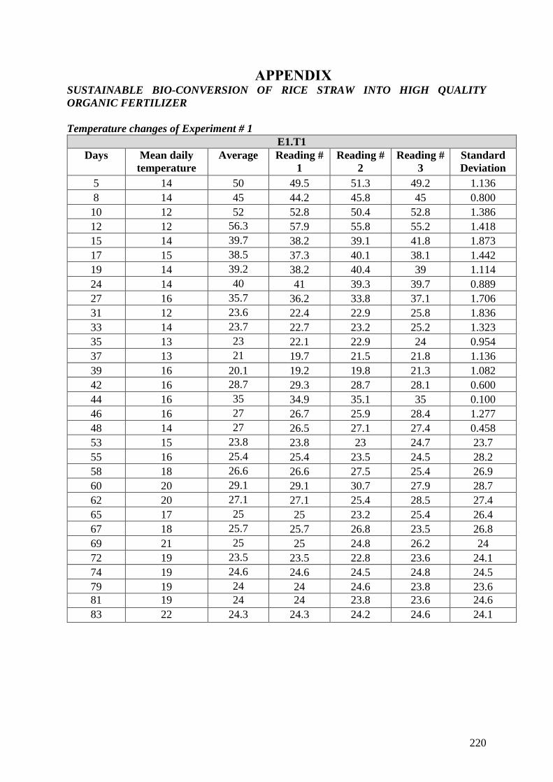
220
APPENDIX SUSTAINABLE BIO-CONVERSION OF RICE STRAW INTO HIGH QUALITY
ORGANIC FERTILIZER
Temperature changes of Experiment # 1
E1.T1
Days Mean daily
temperature
Average Reading #
1
Reading #
2
Reading #
3
Standard
Deviation
5 14 50 49.5 51.3 49.2 1.136
8 14 45 44.2 45.8 45 0.800
10 12 52 52.8 50.4 52.8 1.386
12 12 56.3 57.9 55.8 55.2 1.418
15 14 39.7 38.2 39.1 41.8 1.873
17 15 38.5 37.3 40.1 38.1 1.442
19 14 39.2 38.2 40.4 39 1.114
24 14 40 41 39.3 39.7 0.889
27 16 35.7 36.2 33.8 37.1 1.706
31 12 23.6 22.4 22.9 25.8 1.836
33 14 23.7 22.7 23.2 25.2 1.323
35 13 23 22.1 22.9 24 0.954
37 13 21 19.7 21.5 21.8 1.136
39 16 20.1 19.2 19.8 21.3 1.082
42 16 28.7 29.3 28.7 28.1 0.600
44 16 35 34.9 35.1 35 0.100
46 16 27 26.7 25.9 28.4 1.277
48 14 27 26.5 27.1 27.4 0.458
53 15 23.8 23.8 23 24.7 23.7
55 16 25.4 25.4 23.5 24.5 28.2
58 18 26.6 26.6 27.5 25.4 26.9
60 20 29.1 29.1 30.7 27.9 28.7
62 20 27.1 27.1 25.4 28.5 27.4
65 17 25 25 23.2 25.4 26.4
67 18 25.7 25.7 26.8 23.5 26.8
69 21 25 25 24.8 26.2 24
72 19 23.5 23.5 22.8 23.6 24.1
74 19 24.6 24.6 24.5 24.8 24.5
79 19 24 24 24.6 23.8 23.6
81 19 24 24 23.8 23.6 24.6
83 22 24.3 24.3 24.2 24.6 24.1
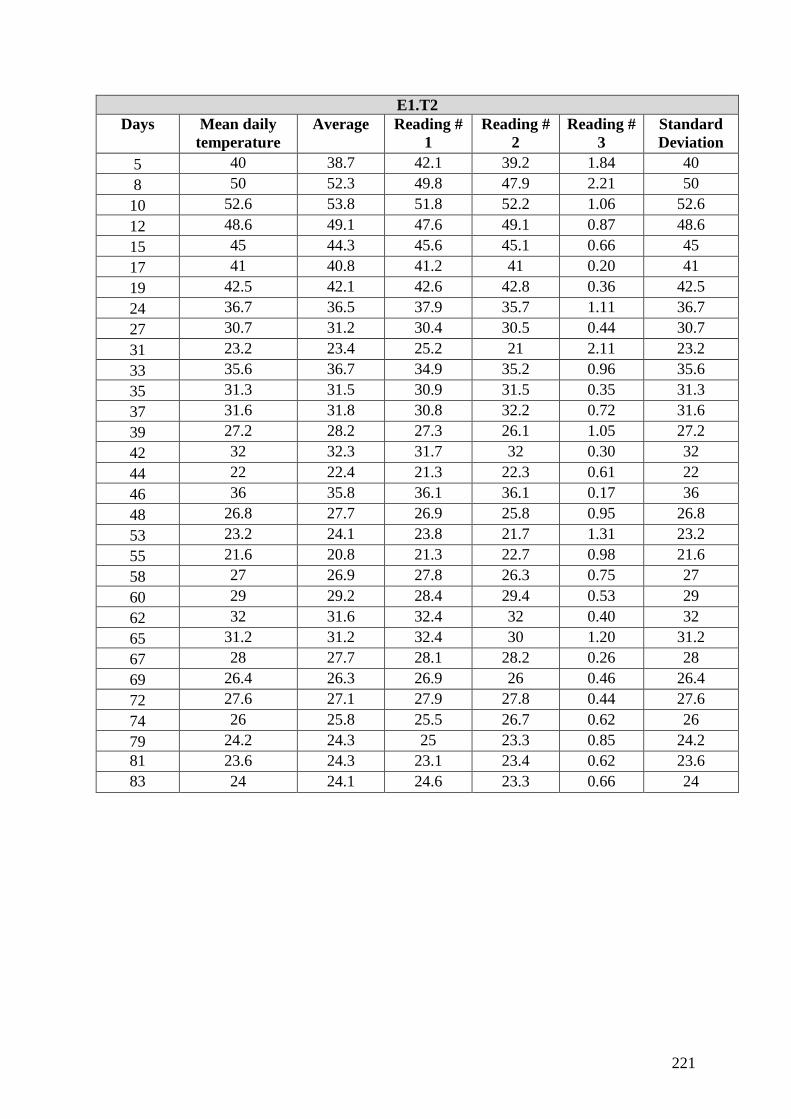
221
E1.T2
Days Mean daily
temperature
Average Reading #
1
Reading #
2
Reading #
3
Standard
Deviation
5 40 38.7 42.1 39.2 1.84 40
8 50 52.3 49.8 47.9 2.21 50
10 52.6 53.8 51.8 52.2 1.06 52.6
12 48.6 49.1 47.6 49.1 0.87 48.6
15 45 44.3 45.6 45.1 0.66 45
17 41 40.8 41.2 41 0.20 41
19 42.5 42.1 42.6 42.8 0.36 42.5
24 36.7 36.5 37.9 35.7 1.11 36.7
27 30.7 31.2 30.4 30.5 0.44 30.7
31 23.2 23.4 25.2 21 2.11 23.2
33 35.6 36.7 34.9 35.2 0.96 35.6
35 31.3 31.5 30.9 31.5 0.35 31.3
37 31.6 31.8 30.8 32.2 0.72 31.6
39 27.2 28.2 27.3 26.1 1.05 27.2
42 32 32.3 31.7 32 0.30 32
44 22 22.4 21.3 22.3 0.61 22
46 36 35.8 36.1 36.1 0.17 36
48 26.8 27.7 26.9 25.8 0.95 26.8
53 23.2 24.1 23.8 21.7 1.31 23.2
55 21.6 20.8 21.3 22.7 0.98 21.6
58 27 26.9 27.8 26.3 0.75 27
60 29 29.2 28.4 29.4 0.53 29
62 32 31.6 32.4 32 0.40 32
65 31.2 31.2 32.4 30 1.20 31.2
67 28 27.7 28.1 28.2 0.26 28
69 26.4 26.3 26.9 26 0.46 26.4
72 27.6 27.1 27.9 27.8 0.44 27.6
74 26 25.8 25.5 26.7 0.62 26
79 24.2 24.3 25 23.3 0.85 24.2
81 23.6 24.3 23.1 23.4 0.62 23.6
83 24 24.1 24.6 23.3 0.66 24
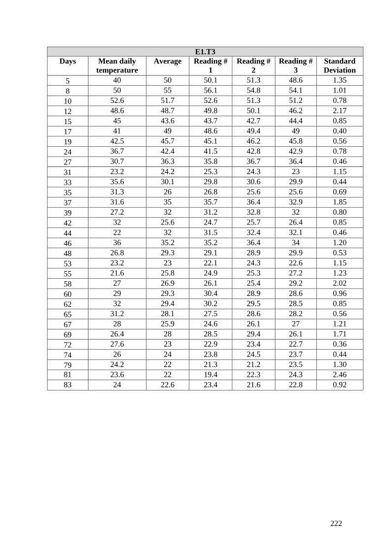
222
E1.T3
Days Mean daily
temperature
Average Reading #
1
Reading #
2
Reading #
3
Standard
Deviation
5 40 50 50.1 51.3 48.6 1.35
8 50 55 56.1 54.8 54.1 1.01
10 52.6 51.7 52.6 51.3 51.2 0.78
12 48.6 48.7 49.8 50.1 46.2 2.17
15 45 43.6 43.7 42.7 44.4 0.85
17 41 49 48.6 49.4 49 0.40
19 42.5 45.7 45.1 46.2 45.8 0.56
24 36.7 42.4 41.5 42.8 42.9 0.78
27 30.7 36.3 35.8 36.7 36.4 0.46
31 23.2 24.2 25.3 24.3 23 1.15
33 35.6 30.1 29.8 30.6 29.9 0.44
35 31.3 26 26.8 25.6 25.6 0.69
37 31.6 35 35.7 36.4 32.9 1.85
39 27.2 32 31.2 32.8 32 0.80
42 32 25.6 24.7 25.7 26.4 0.85
44 22 32 31.5 32.4 32.1 0.46
46 36 35.2 35.2 36.4 34 1.20
48 26.8 29.3 29.1 28.9 29.9 0.53
53 23.2 23 22.1 24.3 22.6 1.15
55 21.6 25.8 24.9 25.3 27.2 1.23
58 27 26.9 26.1 25.4 29.2 2.02
60 29 29.3 30.4 28.9 28.6 0.96
62 32 29.4 30.2 29.5 28.5 0.85
65 31.2 28.1 27.5 28.6 28.2 0.56
67 28 25.9 24.6 26.1 27 1.21
69 26.4 28 28.5 29.4 26.1 1.71
72 27.6 23 22.9 23.4 22.7 0.36
74 26 24 23.8 24.5 23.7 0.44
79 24.2 22 21.3 21.2 23.5 1.30
81 23.6 22 19.4 22.3 24.3 2.46
83 24 22.6 23.4 21.6 22.8 0.92
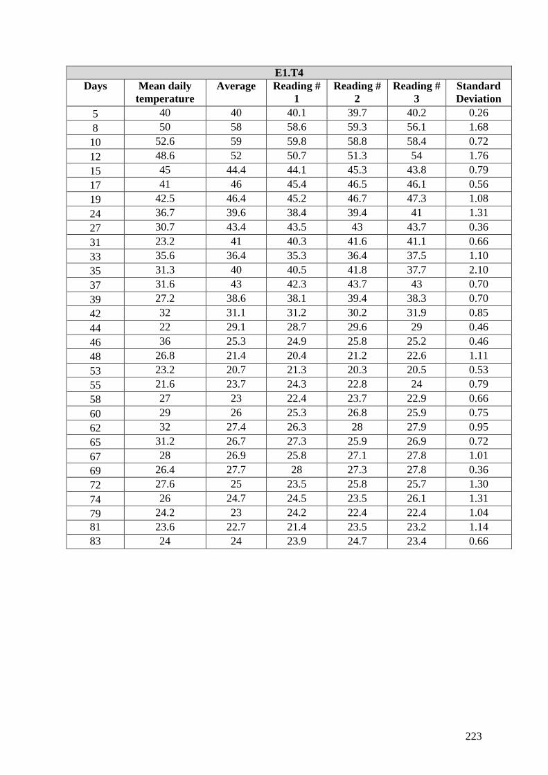
223
E1.T4
Days Mean daily
temperature
Average Reading #
1
Reading #
2
Reading #
3
Standard
Deviation
5 40 40 40.1 39.7 40.2 0.26
8 50 58 58.6 59.3 56.1 1.68
10 52.6 59 59.8 58.8 58.4 0.72
12 48.6 52 50.7 51.3 54 1.76
15 45 44.4 44.1 45.3 43.8 0.79
17 41 46 45.4 46.5 46.1 0.56
19 42.5 46.4 45.2 46.7 47.3 1.08
24 36.7 39.6 38.4 39.4 41 1.31
27 30.7 43.4 43.5 43 43.7 0.36
31 23.2 41 40.3 41.6 41.1 0.66
33 35.6 36.4 35.3 36.4 37.5 1.10
35 31.3 40 40.5 41.8 37.7 2.10
37 31.6 43 42.3 43.7 43 0.70
39 27.2 38.6 38.1 39.4 38.3 0.70
42 32 31.1 31.2 30.2 31.9 0.85
44 22 29.1 28.7 29.6 29 0.46
46 36 25.3 24.9 25.8 25.2 0.46
48 26.8 21.4 20.4 21.2 22.6 1.11
53 23.2 20.7 21.3 20.3 20.5 0.53
55 21.6 23.7 24.3 22.8 24 0.79
58 27 23 22.4 23.7 22.9 0.66
60 29 26 25.3 26.8 25.9 0.75
62 32 27.4 26.3 28 27.9 0.95
65 31.2 26.7 27.3 25.9 26.9 0.72
67 28 26.9 25.8 27.1 27.8 1.01
69 26.4 27.7 28 27.3 27.8 0.36
72 27.6 25 23.5 25.8 25.7 1.30
74 26 24.7 24.5 23.5 26.1 1.31
79 24.2 23 24.2 22.4 22.4 1.04
81 23.6 22.7 21.4 23.5 23.2 1.14
83 24 24 23.9 24.7 23.4 0.66
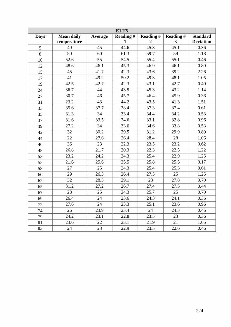
224
E1.T5
Days Mean daily
temperature
Average Reading #
1
Reading #
2
Reading #
3
Standard
Deviation
5 40 45 44.6 45.3 45.1 0.36
8 50 60 61.3 59.7 59 1.18
10 52.6 55 54.5 55.4 55.1 0.46
12 48.6 46.1 45.3 46.9 46.1 0.80
15 45 41.7 42.3 43.6 39.2 2.26
17 41 49.2 50.2 49.3 48.1 1.05
19 42.5 42.7 42.3 43.1 42.7 0.40
24 36.7 44 43.5 45.3 43.2 1.14
27 30.7 46 45.7 46.4 45.9 0.36
31 23.2 43 44.2 43.5 41.3 1.51
33 35.6 37.7 38.4 37.3 37.4 0.61
35 31.3 34 33.4 34.4 34.2 0.53
37 31.6 33.5 34.6 33.1 32.8 0.96
39 27.2 34 33.6 34.6 33.8 0.53
42 32 30.2 29.5 31.2 29.9 0.89
44 22 27.6 26.4 28.4 28 1.06
46 36 23 22.3 23.5 23.2 0.62
48 26.8 21.7 20.3 22.3 22.5 1.22
53 23.2 24.2 24.3 25.4 22.9 1.25
55 21.6 25.6 25.5 25.8 25.5 0.17
58 27 25 24.3 25.4 25.3 0.61
60 29 26.3 26.4 27.5 25 1.25
62 32 28.3 29.1 28 27.8 0.70
65 31.2 27.2 26.7 27.4 27.5 0.44
67 28 25 24.3 25.7 25 0.70
69 26.4 24 23.6 24.3 24.1 0.36
72 27.6 24 23.3 25.1 23.6 0.96
74 26 23.9 23.4 24 24.3 0.46
79 24.2 23.1 22.8 23.5 23 0.36
81 23.6 22 23.1 21.9 21 1.05
83 24 23 22.9 23.5 22.6 0.46
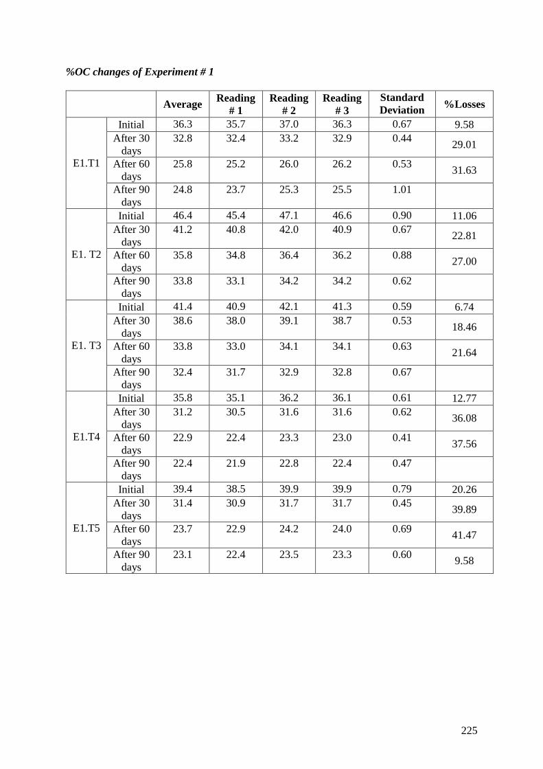
225
%OC changes of Experiment # 1
Average
Reading
# 1
Reading
# 2
Reading
# 3
Standard
Deviation %Losses
E1.T1
Initial 36.3 35.7 37.0 36.3 0.67 9.58
After 30
days
32.8 32.4 33.2 32.9 0.44 29.01
After 60
days
25.8 25.2 26.0 26.2 0.53 31.63
After 90
days
24.8 23.7 25.3 25.5 1.01
E1. T2
Initial 46.4 45.4 47.1 46.6 0.90 11.06
After 30
days
41.2 40.8 42.0 40.9 0.67 22.81
After 60
days
35.8 34.8 36.4 36.2 0.88 27.00
After 90
days
33.8 33.1 34.2 34.2 0.62
E1. T3
Initial 41.4 40.9 42.1 41.3 0.59 6.74
After 30
days
38.6 38.0 39.1 38.7 0.53 18.46
After 60
days
33.8 33.0 34.1 34.1 0.63 21.64
After 90
days
32.4 31.7 32.9 32.8 0.67
E1.T4
Initial 35.8 35.1 36.2 36.1 0.61 12.77
After 30
days
31.2 30.5 31.6 31.6 0.62 36.08
After 60
days
22.9 22.4 23.3 23.0 0.41 37.56
After 90
days
22.4 21.9 22.8 22.4 0.47
E1.T5
Initial 39.4 38.5 39.9 39.9 0.79 20.26
After 30
days
31.4 30.9 31.7 31.7 0.45 39.89
After 60
days
23.7 22.9 24.2 24.0 0.69 41.47
After 90
days
23.1 22.4 23.5 23.3 0.60 9.58
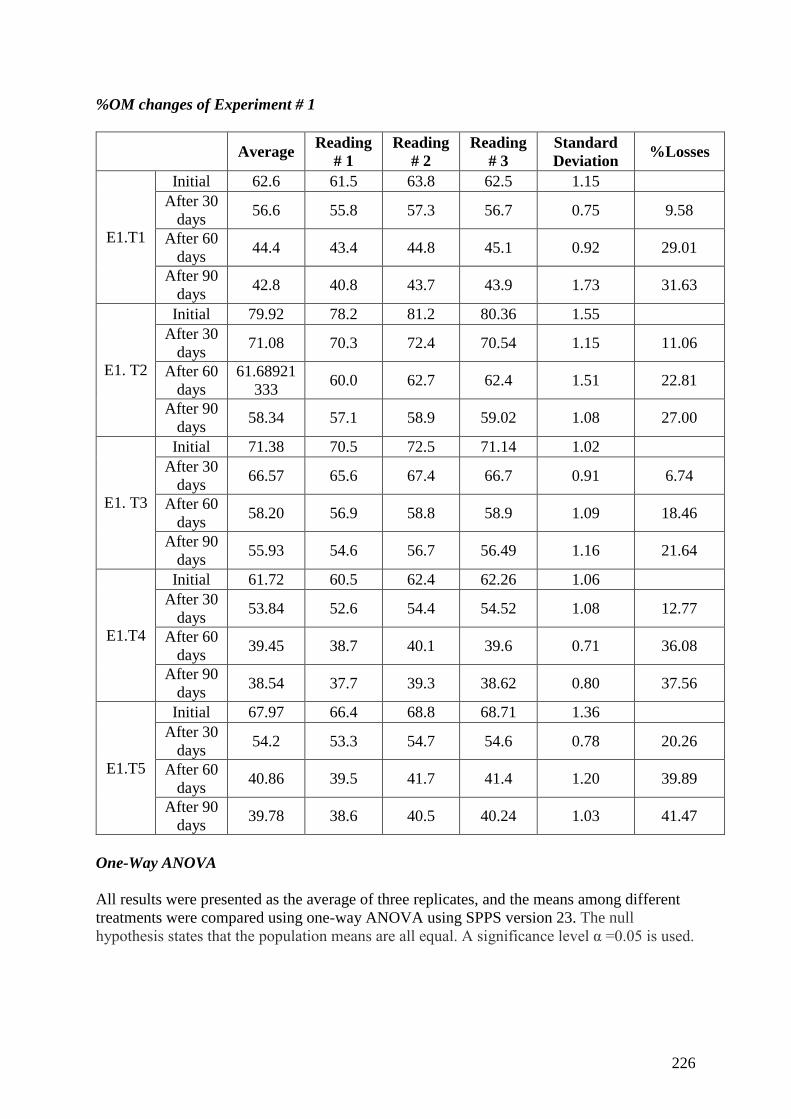
226
%OM changes of Experiment # 1
Average
Reading
# 1
Reading
# 2
Reading
# 3
Standard
Deviation %Losses
E1.T1
Initial 62.6 61.5 63.8 62.5 1.15
After 30
days 56.6 55.8 57.3 56.7 0.75 9.58
After 60
days 44.4 43.4 44.8 45.1 0.92 29.01
After 90
days 42.8 40.8 43.7 43.9 1.73 31.63
E1. T2
Initial 79.92 78.2 81.2 80.36 1.55
After 30
days 71.08 70.3 72.4 70.54 1.15 11.06
After 60
days
61.68921
333 60.0 62.7 62.4 1.51 22.81
After 90
days 58.34 57.1 58.9 59.02 1.08 27.00
E1. T3
Initial 71.38 70.5 72.5 71.14 1.02
After 30
days 66.57 65.6 67.4 66.7 0.91 6.74
After 60
days 58.20 56.9 58.8 58.9 1.09 18.46
After 90
days 55.93 54.6 56.7 56.49 1.16 21.64
E1.T4
Initial 61.72 60.5 62.4 62.26 1.06
After 30
days 53.84 52.6 54.4 54.52 1.08 12.77
After 60
days 39.45 38.7 40.1 39.6 0.71 36.08
After 90
days 38.54 37.7 39.3 38.62 0.80 37.56
E1.T5
Initial 67.97 66.4 68.8 68.71 1.36
After 30
days 54.2 53.3 54.7 54.6 0.78 20.26
After 60
days 40.86 39.5 41.7 41.4 1.20 39.89
After 90
days 39.78 38.6 40.5 40.24 1.03 41.47
One-Way ANOVA
All results were presented as the average of three replicates, and the means among different
treatments were compared using one-way ANOVA using SPPS version 23. The null
hypothesis states that the population means are all equal. A significance level α =0.05 is used.
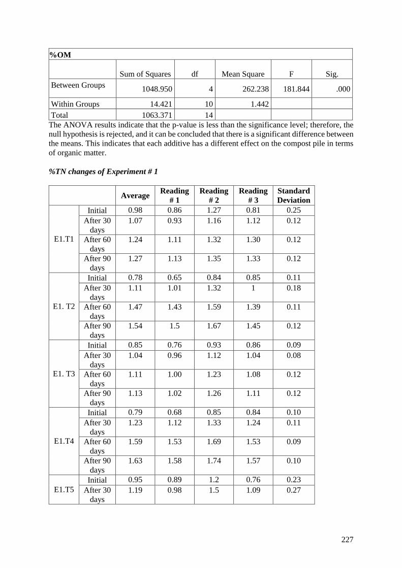
227
%OM
Sum of Squares df Mean Square F Sig.
Between Groups 1048.950 4 262.238 181.844 .000
Within Groups 14.421 10 1.442
Total 1063.371 14
The ANOVA results indicate that the p-value is less than the significance level; therefore, the
null hypothesis is rejected, and it can be concluded that there is a significant difference between
the means. This indicates that each additive has a different effect on the compost pile in terms
of organic matter.
%TN changes of Experiment # 1
Average
Reading
# 1
Reading
# 2
Reading
# 3
Standard
Deviation
E1.T1
Initial 0.98 0.86 1.27 0.81 0.25
After 30
days
1.07 0.93 1.16 1.12 0.12
After 60
days
1.24 1.11 1.32 1.30 0.12
After 90
days
1.27 1.13 1.35 1.33 0.12
E1. T2
Initial 0.78 0.65 0.84 0.85 0.11
After 30
days
1.11 1.01 1.32 1 0.18
After 60
days
1.47 1.43 1.59 1.39 0.11
After 90
days
1.54 1.5 1.67 1.45 0.12
E1. T3
Initial 0.85 0.76 0.93 0.86 0.09
After 30
days
1.04 0.96 1.12 1.04 0.08
After 60
days
1.11 1.00 1.23 1.08 0.12
After 90
days
1.13 1.02 1.26 1.11 0.12
E1.T4
Initial 0.79 0.68 0.85 0.84 0.10
After 30
days
1.23 1.12 1.33 1.24 0.11
After 60
days
1.59 1.53 1.69 1.53 0.09
After 90
days
1.63 1.58 1.74 1.57 0.10
E1.T5
Initial 0.95 0.89 1.2 0.76 0.23
After 30
days
1.19 0.98 1.5 1.09 0.27
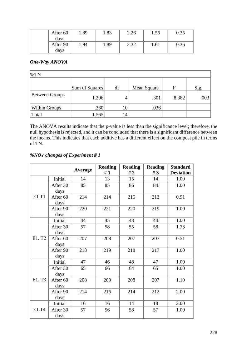
228
After 60
days
1.89 1.83 2.26 1.56 0.35
After 90
days
1.94 1.89 2.32 1.61 0.36
One-Way ANOVA
%TN
Sum of Squares df Mean Square F Sig.
Between Groups 1.206 4 .301 8.382 .003
Within Groups .360 10 .036
Total 1.565 14
The ANOVA results indicate that the p-value is less than the significance level; therefore, the
null hypothesis is rejected, and it can be concluded that there is a significant difference between
the means. This indicates that each additive has a different effect on the compost pile in terms
of TN.
%NO3- changes of Experiment # 1
Average
Reading
# 1
Reading
# 2
Reading
# 3
Standard
Deviation
E1.T1
Initial 14 13 15 14 1.00
After 30
days
85 85 86 84 1.00
After 60
days
214 214 215 213 0.91
After 90
days
220 221 220 219 1.00
E1. T2
Initial 44 45 43 44 1.00
After 30
days
57 58 55 58 1.73
After 60
days
207 208 207 207 0.51
After 90
days
218 219 218 217 1.00
E1. T3
Initial 47 46 48 47 1.00
After 30
days
65 66 64 65 1.00
After 60
days
208 209 208 207 1.10
After 90
days
214 216 214 212 2.00
E1.T4
Initial 16 16 14 18 2.00
After 30
days
57 56 58 57 1.00

229
After 60
days
225 227 223 225 1.94
After 90
days
230 231 228 231 1.73
E1.T5
Initial 18 17 18 19 1.00
After 30
days
106 107 104 107 1.73
After 60
days
289 290 287 289 1.30
After 90
days
295 295 294 296 1.00
%NH4+ changes of Experiment # 1
Average
Reading
# 1
Reading
# 2
Reading
# 3
Standard
Deviation
E1.T1
Initial 376 374 377 377 1.7
After 30
days
187 186 188 187 1.0
After 60
days
36 36 37 35 1.0
After 90
days
35 35 36 34 1.0
E1. T2
Initial 314 313 314 315 1.0
After 30
days
120 118 120 122 2.0
After 60
days
62 61 63 61 0.9
After 90
days
59 58 60 59 1.0
E1. T3
Initial 323 322 324 323 1.0
After 30
days
126 125 126 127 1.0
After 60
days
65 64 66 64 0.9
After 90
days
62 61 63 62 1.0
E1.T4
Initial 410 408 410 412 2.0
After 30
days
234 235 236 231 2.6
After 60
days
33 33 34 32 1.0
After 90
days
32 32 33 31 1.0
E1.T5
Initial 422 421 422 423 1.0
After 30
days
260 261 260 259 1.0
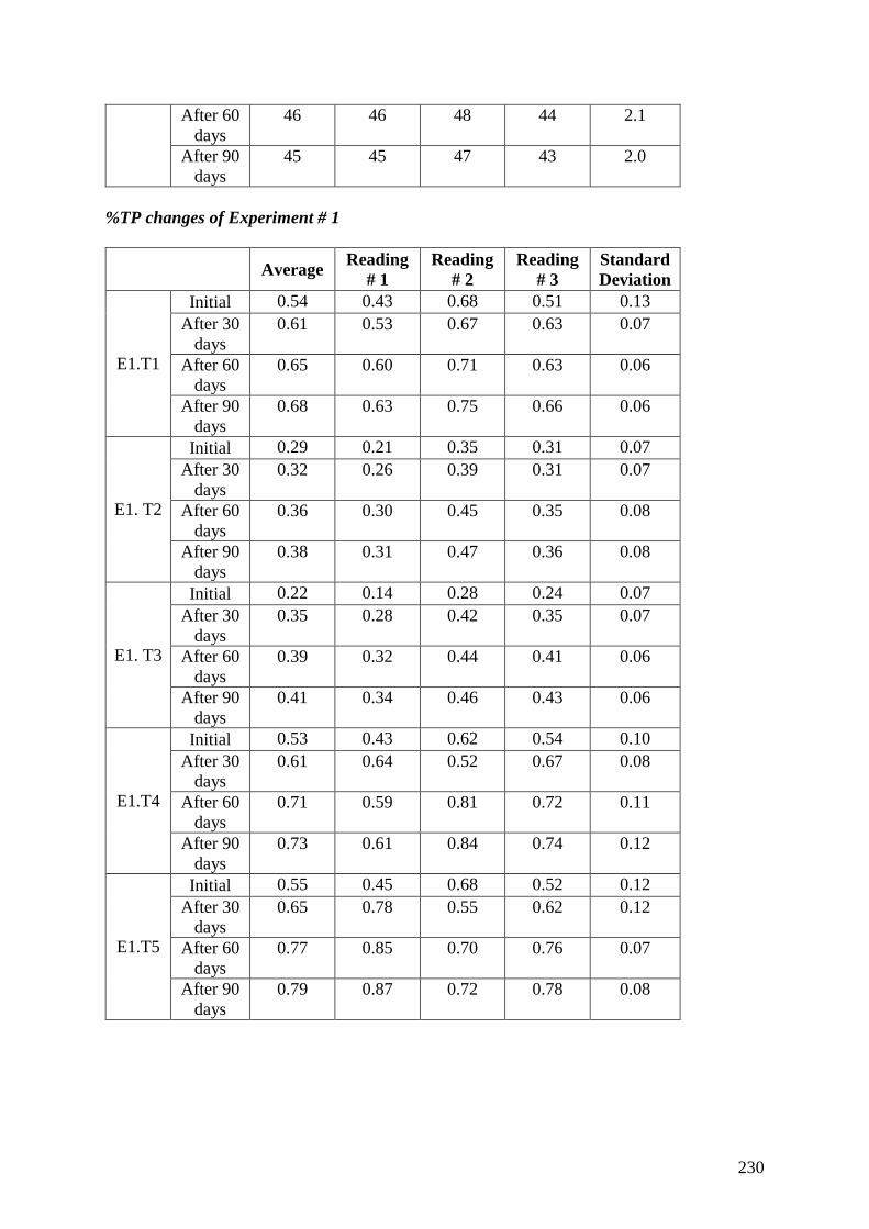
230
After 60
days
46 46 48 44 2.1
After 90
days
45 45 47 43 2.0
%TP changes of Experiment # 1
Average
Reading
# 1
Reading
# 2
Reading
# 3
Standard
Deviation
E1.T1
Initial 0.54 0.43 0.68 0.51 0.13
After 30
days
0.61 0.53 0.67 0.63 0.07
After 60
days
0.65 0.60 0.71 0.63 0.06
After 90
days
0.68 0.63 0.75 0.66 0.06
E1. T2
Initial 0.29 0.21 0.35 0.31 0.07
After 30
days
0.32 0.26 0.39 0.31 0.07
After 60
days
0.36 0.30 0.45 0.35 0.08
After 90
days
0.38 0.31 0.47 0.36 0.08
E1. T3
Initial 0.22 0.14 0.28 0.24 0.07
After 30
days
0.35 0.28 0.42 0.35 0.07
After 60
days
0.39 0.32 0.44 0.41 0.06
After 90
days
0.41 0.34 0.46 0.43 0.06
E1.T4
Initial 0.53 0.43 0.62 0.54 0.10
After 30
days
0.61 0.64 0.52 0.67 0.08
After 60
days
0.71 0.59 0.81 0.72 0.11
After 90
days
0.73 0.61 0.84 0.74 0.12
E1.T5
Initial 0.55 0.45 0.68 0.52 0.12
After 30
days
0.65 0.78 0.55 0.62 0.12
After 60
days
0.77 0.85 0.70 0.76 0.07
After 90
days
0.79 0.87 0.72 0.78 0.08

231
One-Way ANOVA
%TP
Sum of Squares df Mean Square F Sig.
Between Groups .432 4 .108 16.106 .000
Within Groups .067 10 .007
Total .499 14
The ANOVA results indicate that the p-value is less than the significance level; therefore, the
null hypothesis is rejected, and it can be concluded that there is a significant difference between
the means. This indicates that each additive has a different effect on the compost pile in terms
of TP.
%TK changes of Experiment # 1
Average
Reading
# 1
Reading
# 2
Reading
# 3
Standard
Deviation
E1.T1
Initial 0.58 0.51 0.68 0.55 0.09
After 30
days
0.73 0.63 0.82 0.74 0.10
After 60
days
0.78 0.71 0.86 0.76 0.08
After 90
days
0.82 0.75 0.91 0.8 0.08
E1. T2
Initial 0.2 0.15 0.27 0.18 0.06
After 30
days
0.37 0.24 0.46 0.41 0.12
After 60
days
0.48 0.40 0.55 0.48 0.076
After 90
days
0.5 0.42 0.58 0.5 0.08
E1. T3
Initial 0.34 0.28 0.44 0.3 0.09
After 30
days
0.52 0.48 0.64 0.44 0.11
After 60
days
0.68 0.58 0.74 0.73 0.089
After 90
days
0.72 0.61 0.78 0.77 0.10
E1.T4
Initial 0.37 0.28 0.43 0.4 0.08
After 30
days
0.54 0.42 0.59 0.61 0.10
After 60
days
0.79 0.71 0.85 0.80 0.074
After 90
days
0.81 0.73 0.88 0.82 0.08
E1.T5 Initial 0.42 0.34 0.47 0.45 0.07
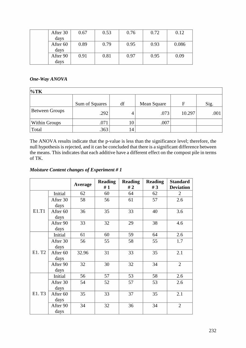
232
After 30
days
0.67 0.53 0.76 0.72 0.12
After 60
days
0.89 0.79 0.95 0.93 0.086
After 90
days
0.91 0.81 0.97 0.95 0.09
One-Way ANOVA
%TK
Sum of Squares df Mean Square F Sig.
Between Groups .292 4 .073 10.297 .001
Within Groups .071 10 .007
Total .363 14
The ANOVA results indicate that the p-value is less than the significance level; therefore, the
null hypothesis is rejected, and it can be concluded that there is a significant difference between
the means. This indicates that each additive have a different effect on the compost pile in terms
of TK.
Moisture Content changes of Experiment # 1
Average
Reading
# 1
Reading
# 2
Reading
# 3
Standard
Deviation
E1.T1
Initial 62 60 64 62 2
After 30
days
58 56 61 57 2.6
After 60
days
36 35 33 40 3.6
After 90
days
33 32 29 38 4.6
E1. T2
Initial 61 60 59 64 2.6
After 30
days
56 55 58 55 1.7
After 60
days
32.96 31 33 35 2.1
After 90
days
32 30 32 34 2
E1. T3
Initial 56 57 53 58 2.6
After 30
days
54 52 57 53 2.6
After 60
days
35 33 37 35 2.1
After 90
days
34 32 36 34 2
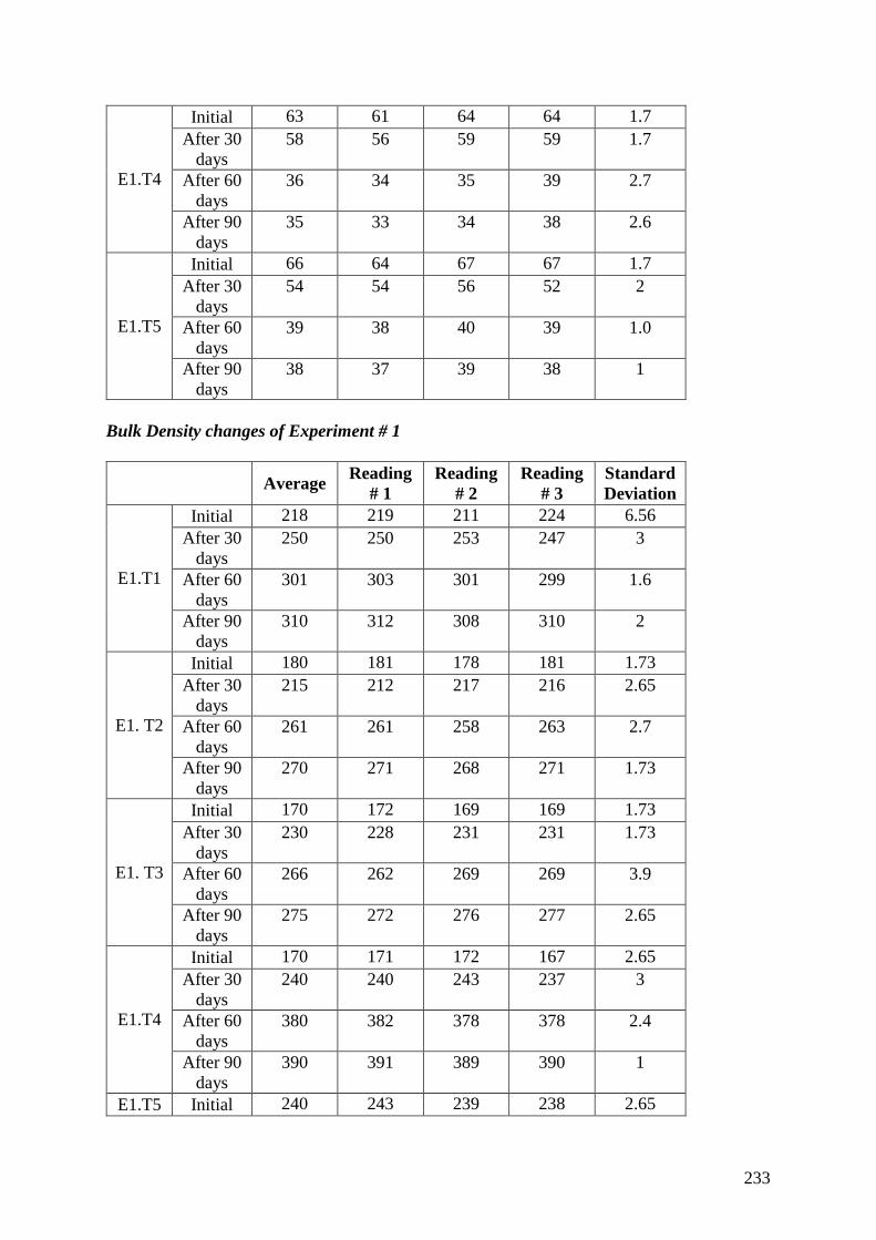
233
E1.T4
Initial 63 61 64 64 1.7
After 30
days
58 56 59 59 1.7
After 60
days
36 34 35 39 2.7
After 90
days
35 33 34 38 2.6
E1.T5
Initial 66 64 67 67 1.7
After 30
days
54 54 56 52 2
After 60
days
39 38 40 39 1.0
After 90
days
38 37 39 38 1
Bulk Density changes of Experiment # 1
Average
Reading
# 1
Reading
# 2
Reading
# 3
Standard
Deviation
E1.T1
Initial 218 219 211 224 6.56
After 30
days
250 250 253 247 3
After 60
days
301 303 301 299 1.6
After 90
days
310 312 308 310 2
E1. T2
Initial 180 181 178 181 1.73
After 30
days
215 212 217 216 2.65
After 60
days
261 261 258 263 2.7
After 90
days
270 271 268 271 1.73
E1. T3
Initial 170 172 169 169 1.73
After 30
days
230 228 231 231 1.73
After 60
days
266 262 269 269 3.9
After 90
days
275 272 276 277 2.65
E1.T4
Initial 170 171 172 167 2.65
After 30
days
240 240 243 237 3
After 60
days
380 382 378 378 2.4
After 90
days
390 391 389 390 1
E1.T5 Initial 240 243 239 238 2.65
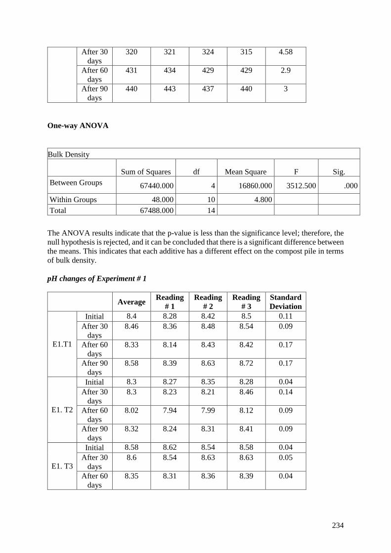
234
After 30
days
320 321 324 315 4.58
After 60
days
431 434 429 429 2.9
After 90
days
440 443 437 440 3
One-way ANOVA
Bulk Density
Sum of Squares df Mean Square F Sig.
Between Groups 67440.000 4 16860.000 3512.500 .000
Within Groups 48.000 10 4.800
Total 67488.000 14
The ANOVA results indicate that the p-value is less than the significance level; therefore, the
null hypothesis is rejected, and it can be concluded that there is a significant difference between
the means. This indicates that each additive has a different effect on the compost pile in terms
of bulk density.
pH changes of Experiment # 1
Average
Reading
# 1
Reading
# 2
Reading
# 3
Standard
Deviation
E1.T1
Initial 8.4 8.28 8.42 8.5 0.11
After 30
days
8.46 8.36 8.48 8.54 0.09
After 60
days
8.33 8.14 8.43 8.42 0.17
After 90
days
8.58 8.39 8.63 8.72 0.17
E1. T2
Initial 8.3 8.27 8.35 8.28 0.04
After 30
days
8.3 8.23 8.21 8.46 0.14
After 60
days
8.02 7.94 7.99 8.12 0.09
After 90
days
8.32 8.24 8.31 8.41 0.09
E1. T3
Initial 8.58 8.62 8.54 8.58 0.04
After 30
days
8.6 8.54 8.63 8.63 0.05
After 60
days
8.35 8.31 8.36 8.39 0.04
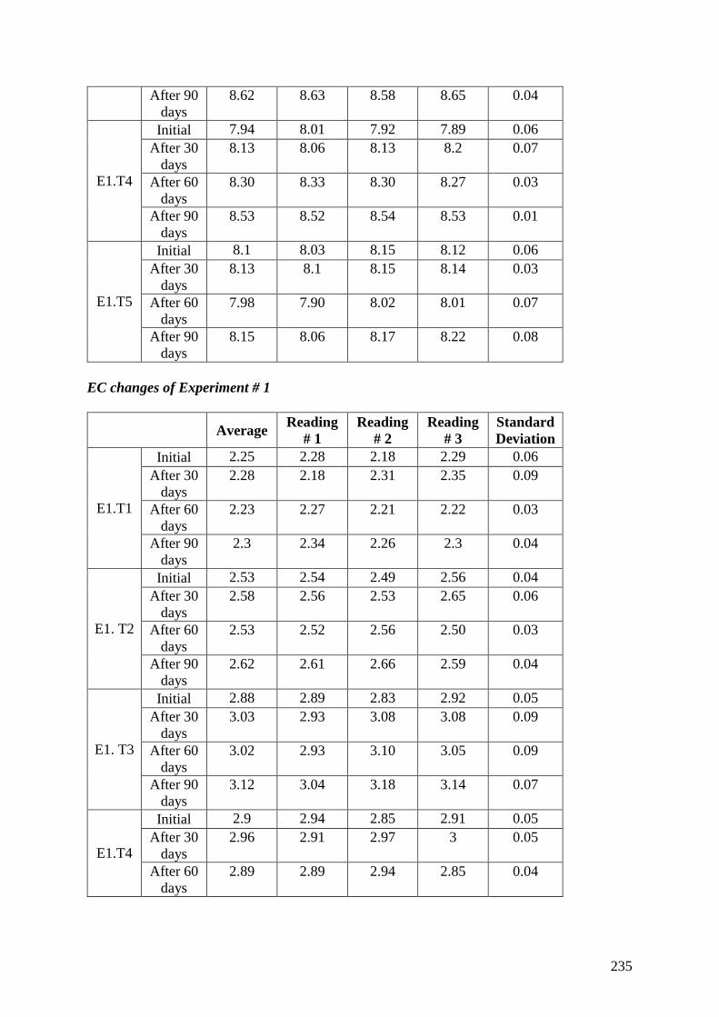
235
After 90
days
8.62 8.63 8.58 8.65 0.04
E1.T4
Initial 7.94 8.01 7.92 7.89 0.06
After 30
days
8.13 8.06 8.13 8.2 0.07
After 60
days
8.30 8.33 8.30 8.27 0.03
After 90
days
8.53 8.52 8.54 8.53 0.01
E1.T5
Initial 8.1 8.03 8.15 8.12 0.06
After 30
days
8.13 8.1 8.15 8.14 0.03
After 60
days
7.98 7.90 8.02 8.01 0.07
After 90
days
8.15 8.06 8.17 8.22 0.08
EC changes of Experiment # 1
Average
Reading
# 1
Reading
# 2
Reading
# 3
Standard
Deviation
E1.T1
Initial 2.25 2.28 2.18 2.29 0.06
After 30
days
2.28 2.18 2.31 2.35 0.09
After 60
days
2.23 2.27 2.21 2.22 0.03
After 90
days
2.3 2.34 2.26 2.3 0.04
E1. T2
Initial 2.53 2.54 2.49 2.56 0.04
After 30
days
2.58 2.56 2.53 2.65 0.06
After 60
days
2.53 2.52 2.56 2.50 0.03
After 90
days
2.62 2.61 2.66 2.59 0.04
E1. T3
Initial 2.88 2.89 2.83 2.92 0.05
After 30
days
3.03 2.93 3.08 3.08 0.09
After 60
days
3.02 2.93 3.10 3.05 0.09
After 90
days
3.12 3.04 3.18 3.14 0.07
E1.T4
Initial 2.9 2.94 2.85 2.91 0.05
After 30
days
2.96 2.91 2.97 3 0.05
After 60
days
2.89 2.89 2.94 2.85 0.04

236
After 90
days
2.97 2.95 3.02 2.94 0.04
E1.T5
Initial 2.39 2.41 2.37 2.39 0.02
After 30
days
2.53 2.51 2.54 2.54 0.02
After 60
days
2.55 2.57 2.53 2.54 0.02
After 90
days
2.6 2.62 2.58 2.6 0.02
Temperature changes of Experiment # 2
E2.T1
Days Mean daily
temperature Average
Reading #
1
Reading #
2
Reading #
3
Standard
Deviation
5 35 67.50 65.9 67.8 68.8 1.47
8 29 62.60 60.5 62.5 64.8 2.15
10 37 51.90 52.5 50.4 52.8 1.31
12 34 48.00 47.8 47.4 48.8 0.72
15 35 48.50 47.6 48.4 49.5 0.95
17 34 59.50 60.3 58.3 59.9 1.06
19 37 53.90 52.4 53.6 55.7 1.67
24 39 49.50 48.6 49.7 50.2 0.82
27 33 46.30 44.7 46.4 47.8 1.55
31 33 46.00 44.7 46.3 47 1.18
33 33 50.60 50.2 52.2 49.4 1.44
35 36 51.00 51.7 50.6 50.7 0.61
37 38 47.00 47.6 46.8 46.6 0.53
39 32 43.00 42.5 43.6 42.9 0.56
42 34 38.50 37.2 38.6 39.7 1.25
44 35 36.50 35.1 36.9 37.5 1.25
46 40 41 40 41.4 41.6 0.87
48 40 40.5 39.4 40.2 41.9 1.28
53 35 36.2 35.7 36.5 36.4 0.44
55 34 35.4 34.9 35.6 35.7 0.44
58 37 36.7 36.1 36.9 37.1 0.53
60 37 36.3 35.9 36.4 36.6 0.36
62 38 36.5 36.2 37.2 36.1 0.61
65 35 36.3 35.7 36.6 36.6 0.52
67 34 35.8 35.2 36.1 36.1 0.52
69 35 36.7 35.8 36.9 37.4 0.82
72 38 37.6 37.9 37.4 37.5 0.26
74 36 37.1 37.4 36.8 37.1 0.30
79 35 36.4 35.8 36.3 37.1 0.66
81 37 36.6 36.1 37.2 36.5 0.56
83 35 36.3 36.1 35.9 36.9 0.53
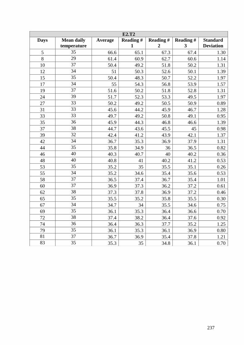
237
E2.T2
Days Mean daily
temperature
Average Reading #
1
Reading #
2
Reading #
3
Standard
Deviation
5 35 66.6 65.1 67.3 67.4 1.30
8 29 61.4 60.9 62.7 60.6 1.14
10 37 50.4 49.2 51.8 50.2 1.31
12 34 51 50.3 52.6 50.1 1.39
15 35 50.4 48.3 50.7 52.2 1.97
17 34 55 54.3 56.8 53.9 1.57
19 37 51.6 50.2 51.8 52.8 1.31
24 39 51.7 52.3 53.3 49.5 1.97
27 33 50.2 49.2 50.5 50.9 0.89
31 33 45.6 44.2 45.9 46.7 1.28
33 33 49.7 49.2 50.8 49.1 0.95
35 36 45.9 44.3 46.8 46.6 1.39
37 38 44.7 43.6 45.5 45 0.98
39 32 42.4 41.2 43.9 42.1 1.37
42 34 36.7 35.3 36.9 37.9 1.31
44 35 35.8 34.9 36 36.5 0.82
46 40 40.3 40.7 40 40.2 0.36
48 40 40.8 41 40.2 41.2 0.53
53 35 35.2 35 35.5 35.1 0.26
55 34 35.2 34.6 35.4 35.6 0.53
58 37 36.5 37.4 36.7 35.4 1.01
60 37 36.9 37.3 36.2 37.2 0.61
62 38 37.3 37.8 36.9 37.2 0.46
65 35 35.5 35.2 35.8 35.5 0.30
67 34 34.7 34 35.5 34.6 0.75
69 35 36.1 35.3 36.4 36.6 0.70
72 38 37.4 38.2 36.4 37.6 0.92
74 36 36.4 36.3 37.7 35.2 1.25
79 35 36.1 35.3 36.1 36.9 0.80
81 37 36.7 36.9 35.4 37.8 1.21
83 35 35.3 35 34.8 36.1 0.70
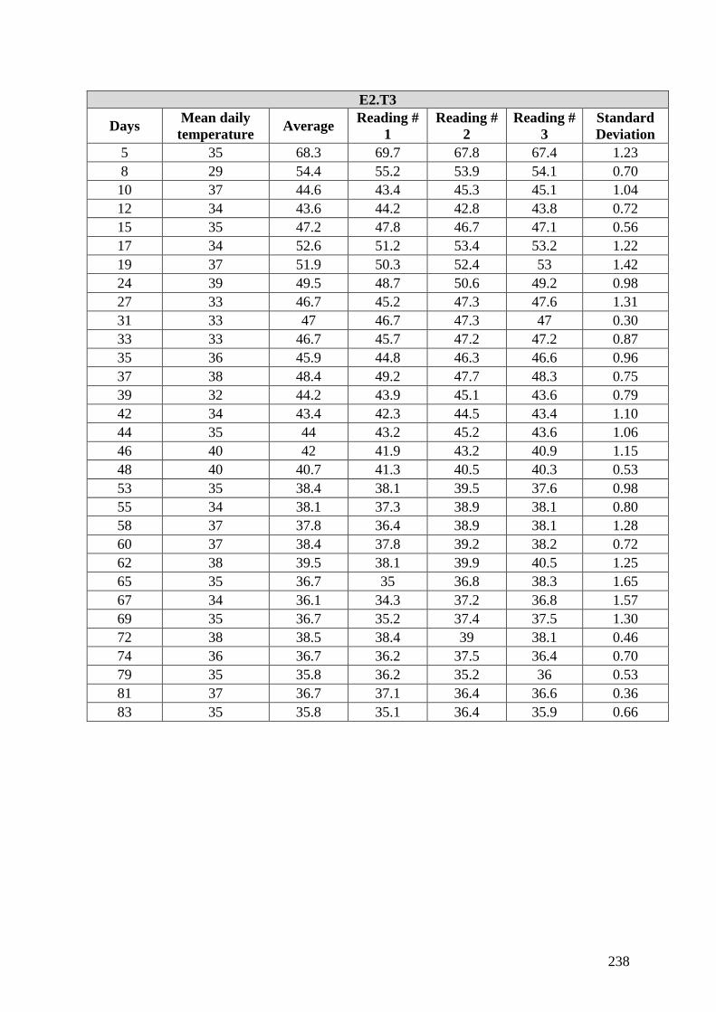
238
E2.T3
Days Mean daily
temperature Average
Reading #
1
Reading #
2
Reading #
3
Standard
Deviation
5 35 68.3 69.7 67.8 67.4 1.23
8 29 54.4 55.2 53.9 54.1 0.70
10 37 44.6 43.4 45.3 45.1 1.04
12 34 43.6 44.2 42.8 43.8 0.72
15 35 47.2 47.8 46.7 47.1 0.56
17 34 52.6 51.2 53.4 53.2 1.22
19 37 51.9 50.3 52.4 53 1.42
24 39 49.5 48.7 50.6 49.2 0.98
27 33 46.7 45.2 47.3 47.6 1.31
31 33 47 46.7 47.3 47 0.30
33 33 46.7 45.7 47.2 47.2 0.87
35 36 45.9 44.8 46.3 46.6 0.96
37 38 48.4 49.2 47.7 48.3 0.75
39 32 44.2 43.9 45.1 43.6 0.79
42 34 43.4 42.3 44.5 43.4 1.10
44 35 44 43.2 45.2 43.6 1.06
46 40 42 41.9 43.2 40.9 1.15
48 40 40.7 41.3 40.5 40.3 0.53
53 35 38.4 38.1 39.5 37.6 0.98
55 34 38.1 37.3 38.9 38.1 0.80
58 37 37.8 36.4 38.9 38.1 1.28
60 37 38.4 37.8 39.2 38.2 0.72
62 38 39.5 38.1 39.9 40.5 1.25
65 35 36.7 35 36.8 38.3 1.65
67 34 36.1 34.3 37.2 36.8 1.57
69 35 36.7 35.2 37.4 37.5 1.30
72 38 38.5 38.4 39 38.1 0.46
74 36 36.7 36.2 37.5 36.4 0.70
79 35 35.8 36.2 35.2 36 0.53
81 37 36.7 37.1 36.4 36.6 0.36
83 35 35.8 35.1 36.4 35.9 0.66
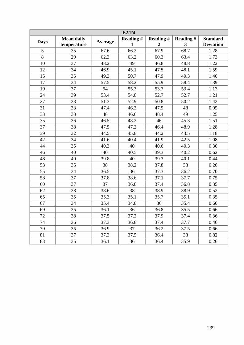
239
E2.T4
Days Mean daily
temperature Average
Reading #
1
Reading #
2
Reading #
3
Standard
Deviation
5 35 67.6 66.2 67.9 68.7 1.28
8 29 62.3 63.2 60.3 63.4 1.73
10 37 48.2 49 46.8 48.8 1.22
12 34 46.9 45.1 47.5 48.1 1.59
15 35 49.3 50.7 47.9 49.3 1.40
17 34 57.5 58.2 55.9 58.4 1.39
19 37 54 55.3 53.3 53.4 1.13
24 39 53.4 54.8 52.7 52.7 1.21
27 33 51.3 52.9 50.8 50.2 1.42
31 33 47.4 46.3 47.9 48 0.95
33 33 48 46.6 48.4 49 1.25
35 36 46.5 48.2 46 45.3 1.51
37 38 47.5 47.2 46.4 48.9 1.28
39 32 44.5 45.8 44.2 43.5 1.18
42 34 41.6 40.4 41.9 42.5 1.08
44 35 40.3 40 40.6 40.3 0.30
46 40 40 40.5 39.3 40.2 0.62
48 40 39.8 40 39.3 40.1 0.44
53 35 38 38.2 37.8 38 0.20
55 34 36.5 36 37.3 36.2 0.70
58 37 37.8 38.6 37.1 37.7 0.75
60 37 37 36.8 37.4 36.8 0.35
62 38 38.6 38 38.9 38.9 0.52
65 35 35.3 35.1 35.7 35.1 0.35
67 34 35.4 34.8 36 35.4 0.60
69 35 36.1 36 36.8 35.5 0.66
72 38 37.5 37.2 37.9 37.4 0.36
74 36 37.3 36.8 37.4 37.7 0.46
79 35 36.9 37 36.2 37.5 0.66
81 37 37.3 37.5 36.4 38 0.82
83 35 36.1 36 36.4 35.9 0.26
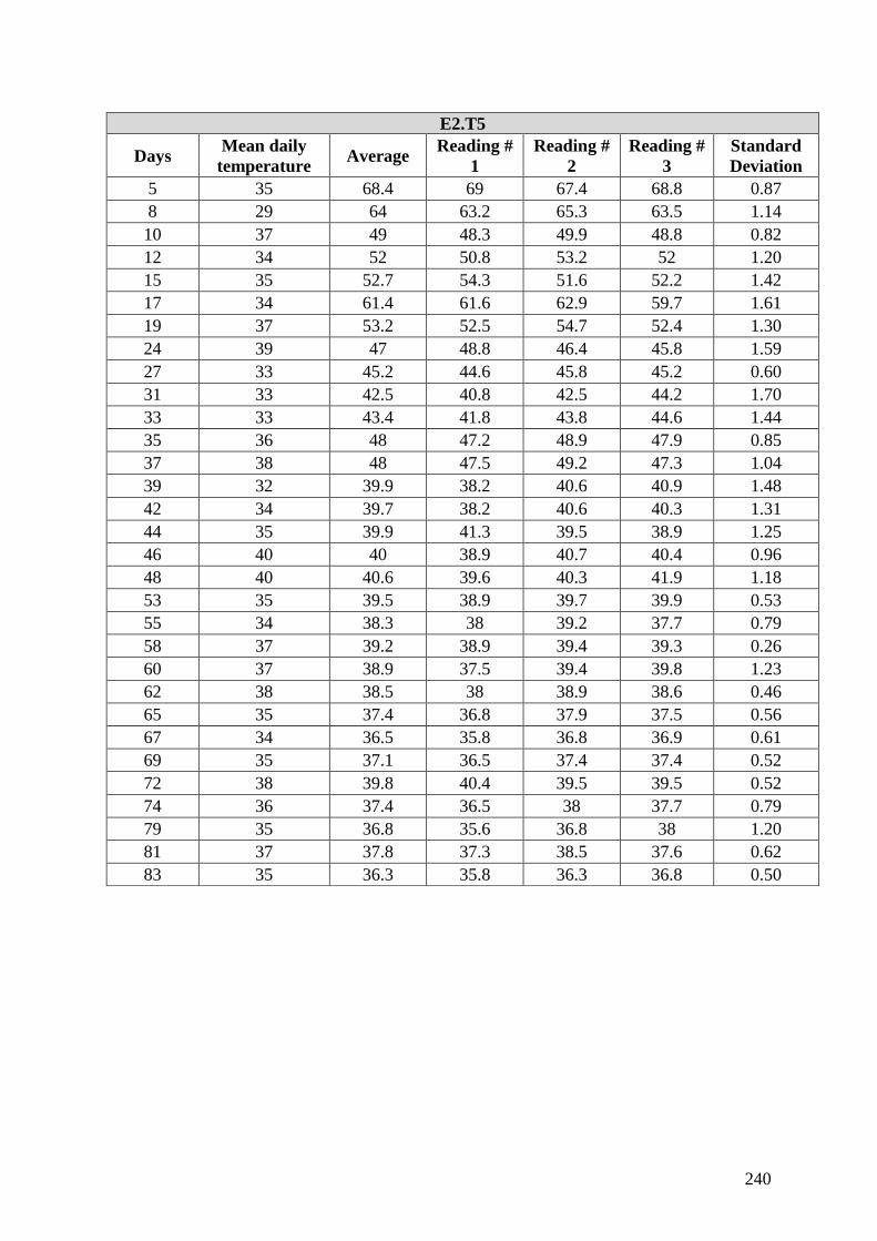
240
E2.T5
Days Mean daily
temperature Average
Reading #
1
Reading #
2
Reading #
3
Standard
Deviation
5 35 68.4 69 67.4 68.8 0.87
8 29 64 63.2 65.3 63.5 1.14
10 37 49 48.3 49.9 48.8 0.82
12 34 52 50.8 53.2 52 1.20
15 35 52.7 54.3 51.6 52.2 1.42
17 34 61.4 61.6 62.9 59.7 1.61
19 37 53.2 52.5 54.7 52.4 1.30
24 39 47 48.8 46.4 45.8 1.59
27 33 45.2 44.6 45.8 45.2 0.60
31 33 42.5 40.8 42.5 44.2 1.70
33 33 43.4 41.8 43.8 44.6 1.44
35 36 48 47.2 48.9 47.9 0.85
37 38 48 47.5 49.2 47.3 1.04
39 32 39.9 38.2 40.6 40.9 1.48
42 34 39.7 38.2 40.6 40.3 1.31
44 35 39.9 41.3 39.5 38.9 1.25
46 40 40 38.9 40.7 40.4 0.96
48 40 40.6 39.6 40.3 41.9 1.18
53 35 39.5 38.9 39.7 39.9 0.53
55 34 38.3 38 39.2 37.7 0.79
58 37 39.2 38.9 39.4 39.3 0.26
60 37 38.9 37.5 39.4 39.8 1.23
62 38 38.5 38 38.9 38.6 0.46
65 35 37.4 36.8 37.9 37.5 0.56
67 34 36.5 35.8 36.8 36.9 0.61
69 35 37.1 36.5 37.4 37.4 0.52
72 38 39.8 40.4 39.5 39.5 0.52
74 36 37.4 36.5 38 37.7 0.79
79 35 36.8 35.6 36.8 38 1.20
81 37 37.8 37.3 38.5 37.6 0.62
83 35 36.3 35.8 36.3 36.8 0.50
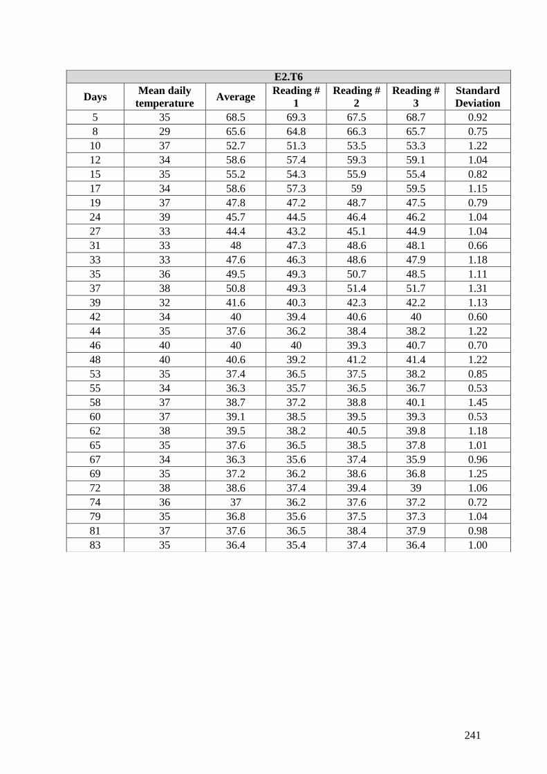
241
E2.T6
Days Mean daily
temperature Average
Reading #
1
Reading #
2
Reading #
3
Standard
Deviation
5 35 68.5 69.3 67.5 68.7 0.92
8 29 65.6 64.8 66.3 65.7 0.75
10 37 52.7 51.3 53.5 53.3 1.22
12 34 58.6 57.4 59.3 59.1 1.04
15 35 55.2 54.3 55.9 55.4 0.82
17 34 58.6 57.3 59 59.5 1.15
19 37 47.8 47.2 48.7 47.5 0.79
24 39 45.7 44.5 46.4 46.2 1.04
27 33 44.4 43.2 45.1 44.9 1.04
31 33 48 47.3 48.6 48.1 0.66
33 33 47.6 46.3 48.6 47.9 1.18
35 36 49.5 49.3 50.7 48.5 1.11
37 38 50.8 49.3 51.4 51.7 1.31
39 32 41.6 40.3 42.3 42.2 1.13
42 34 40 39.4 40.6 40 0.60
44 35 37.6 36.2 38.4 38.2 1.22
46 40 40 40 39.3 40.7 0.70
48 40 40.6 39.2 41.2 41.4 1.22
53 35 37.4 36.5 37.5 38.2 0.85
55 34 36.3 35.7 36.5 36.7 0.53
58 37 38.7 37.2 38.8 40.1 1.45
60 37 39.1 38.5 39.5 39.3 0.53
62 38 39.5 38.2 40.5 39.8 1.18
65 35 37.6 36.5 38.5 37.8 1.01
67 34 36.3 35.6 37.4 35.9 0.96
69 35 37.2 36.2 38.6 36.8 1.25
72 38 38.6 37.4 39.4 39 1.06
74 36 37 36.2 37.6 37.2 0.72
79 35 36.8 35.6 37.5 37.3 1.04
81 37 37.6 36.5 38.4 37.9 0.98
83 35 36.4 35.4 37.4 36.4 1.00
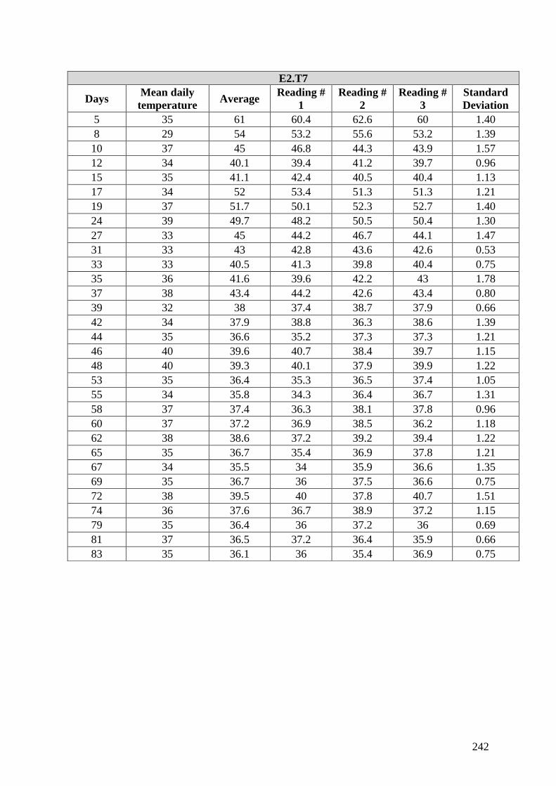
242
E2.T7
Days Mean daily
temperature Average
Reading #
1
Reading #
2
Reading #
3
Standard
Deviation
5 35 61 60.4 62.6 60 1.40
8 29 54 53.2 55.6 53.2 1.39
10 37 45 46.8 44.3 43.9 1.57
12 34 40.1 39.4 41.2 39.7 0.96
15 35 41.1 42.4 40.5 40.4 1.13
17 34 52 53.4 51.3 51.3 1.21
19 37 51.7 50.1 52.3 52.7 1.40
24 39 49.7 48.2 50.5 50.4 1.30
27 33 45 44.2 46.7 44.1 1.47
31 33 43 42.8 43.6 42.6 0.53
33 33 40.5 41.3 39.8 40.4 0.75
35 36 41.6 39.6 42.2 43 1.78
37 38 43.4 44.2 42.6 43.4 0.80
39 32 38 37.4 38.7 37.9 0.66
42 34 37.9 38.8 36.3 38.6 1.39
44 35 36.6 35.2 37.3 37.3 1.21
46 40 39.6 40.7 38.4 39.7 1.15
48 40 39.3 40.1 37.9 39.9 1.22
53 35 36.4 35.3 36.5 37.4 1.05
55 34 35.8 34.3 36.4 36.7 1.31
58 37 37.4 36.3 38.1 37.8 0.96
60 37 37.2 36.9 38.5 36.2 1.18
62 38 38.6 37.2 39.2 39.4 1.22
65 35 36.7 35.4 36.9 37.8 1.21
67 34 35.5 34 35.9 36.6 1.35
69 35 36.7 36 37.5 36.6 0.75
72 38 39.5 40 37.8 40.7 1.51
74 36 37.6 36.7 38.9 37.2 1.15
79 35 36.4 36 37.2 36 0.69
81 37 36.5 37.2 36.4 35.9 0.66
83 35 36.1 36 35.4 36.9 0.75
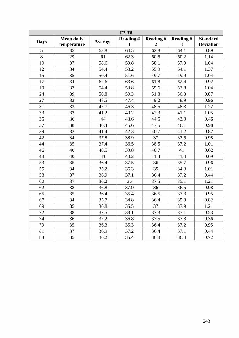
243
E2.T8
Days Mean daily
temperature Average
Reading #
1
Reading #
2
Reading #
3
Standard
Deviation
5 35 63.8 64.5 62.8 64.1 0.89
8 29 61 62.3 60.5 60.2 1.14
10 37 58.6 59.8 58.1 57.9 1.04
12 34 54.4 53.2 55.9 54.1 1.37
15 35 50.4 51.6 49.7 49.9 1.04
17 34 62.6 63.6 61.8 62.4 0.92
19 37 54.4 53.8 55.6 53.8 1.04
24 39 50.8 50.3 51.8 50.3 0.87
27 33 48.5 47.4 49.2 48.9 0.96
31 33 47.7 46.3 48.5 48.3 1.22
33 33 41.2 40.2 42.3 41.1 1.05
35 36 44 43.6 44.5 43.9 0.46
37 38 46.4 45.6 47.5 46.1 0.98
39 32 41.4 42.3 40.7 41.2 0.82
42 34 37.8 38.9 37 37.5 0.98
44 35 37.4 36.5 38.5 37.2 1.01
46 40 40.5 39.8 40.7 41 0.62
48 40 41 40.2 41.4 41.4 0.69
53 35 36.4 37.5 36 35.7 0.96
55 34 35.2 36.3 35 34.3 1.01
58 37 36.9 37.1 36.4 37.2 0.44
60 37 36.2 36 37.5 35.1 1.21
62 38 36.8 37.9 36 36.5 0.98
65 35 36.4 35.4 36.5 37.3 0.95
67 34 35.7 34.8 36.4 35.9 0.82
69 35 36.8 35.5 37 37.9 1.21
72 38 37.5 38.1 37.3 37.1 0.53
74 36 37.2 36.8 37.5 37.3 0.36
79 35 36.3 35.3 36.4 37.2 0.95
81 37 36.9 37.2 36.4 37.1 0.44
83 35 36.2 35.4 36.8 36.4 0.72
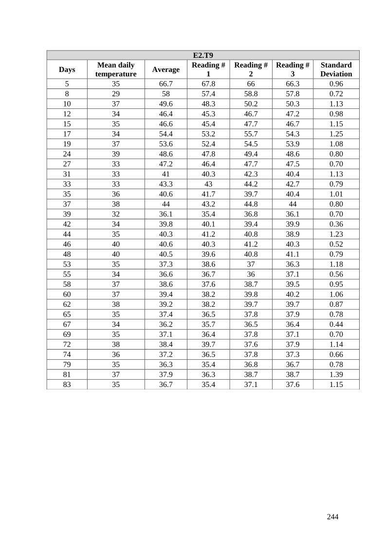
244
E2.T9
Days Mean daily
temperature Average
Reading #
1
Reading #
2
Reading #
3
Standard
Deviation
5 35 66.7 67.8 66 66.3 0.96
8 29 58 57.4 58.8 57.8 0.72
10 37 49.6 48.3 50.2 50.3 1.13
12 34 46.4 45.3 46.7 47.2 0.98
15 35 46.6 45.4 47.7 46.7 1.15
17 34 54.4 53.2 55.7 54.3 1.25
19 37 53.6 52.4 54.5 53.9 1.08
24 39 48.6 47.8 49.4 48.6 0.80
27 33 47.2 46.4 47.7 47.5 0.70
31 33 41 40.3 42.3 40.4 1.13
33 33 43.3 43 44.2 42.7 0.79
35 36 40.6 41.7 39.7 40.4 1.01
37 38 44 43.2 44.8 44 0.80
39 32 36.1 35.4 36.8 36.1 0.70
42 34 39.8 40.1 39.4 39.9 0.36
44 35 40.3 41.2 40.8 38.9 1.23
46 40 40.6 40.3 41.2 40.3 0.52
48 40 40.5 39.6 40.8 41.1 0.79
53 35 37.3 38.6 37 36.3 1.18
55 34 36.6 36.7 36 37.1 0.56
58 37 38.6 37.6 38.7 39.5 0.95
60 37 39.4 38.2 39.8 40.2 1.06
62 38 39.2 38.2 39.7 39.7 0.87
65 35 37.4 36.5 37.8 37.9 0.78
67 34 36.2 35.7 36.5 36.4 0.44
69 35 37.1 36.4 37.8 37.1 0.70
72 38 38.4 39.7 37.6 37.9 1.14
74 36 37.2 36.5 37.8 37.3 0.66
79 35 36.3 35.4 36.8 36.7 0.78
81 37 37.9 36.3 38.7 38.7 1.39
83 35 36.7 35.4 37.1 37.6 1.15
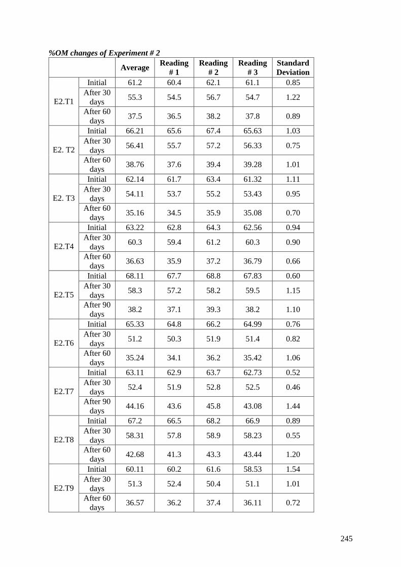
245
%OM changes of Experiment # 2
Average Reading
# 1
Reading
# 2
Reading
# 3
Standard
Deviation
E2.T1
Initial 61.2 60.4 62.1 61.1 0.85
After 30
days 55.3 54.5 56.7 54.7 1.22
After 60
days 37.5 36.5 38.2 37.8 0.89
E2. T2
Initial 66.21 65.6 67.4 65.63 1.03
After 30
days 56.41 55.7 57.2 56.33 0.75
After 60
days 38.76 37.6 39.4 39.28 1.01
E2. T3
Initial 62.14 61.7 63.4 61.32 1.11
After 30
days 54.11 53.7 55.2 53.43 0.95
After 60
days 35.16 34.5 35.9 35.08 0.70
E2.T4
Initial 63.22 62.8 64.3 62.56 0.94
After 30
days 60.3 59.4 61.2 60.3 0.90
After 60
days 36.63 35.9 37.2 36.79 0.66
E2.T5
Initial 68.11 67.7 68.8 67.83 0.60
After 30
days 58.3 57.2 58.2 59.5 1.15
After 90
days 38.2 37.1 39.3 38.2 1.10
E2.T6
Initial 65.33 64.8 66.2 64.99 0.76
After 30
days 51.2 50.3 51.9 51.4 0.82
After 60
days 35.24 34.1 36.2 35.42 1.06
E2.T7
Initial 63.11 62.9 63.7 62.73 0.52
After 30
days 52.4 51.9 52.8 52.5 0.46
After 90
days 44.16 43.6 45.8 43.08 1.44
E2.T8
Initial 67.2 66.5 68.2 66.9 0.89
After 30
days 58.31 57.8 58.9 58.23 0.55
After 60
days 42.68 41.3 43.3 43.44 1.20
E2.T9
Initial 60.11 60.2 61.6 58.53 1.54
After 30
days 51.3 52.4 50.4 51.1 1.01
After 60
days 36.57 36.2 37.4 36.11 0.72
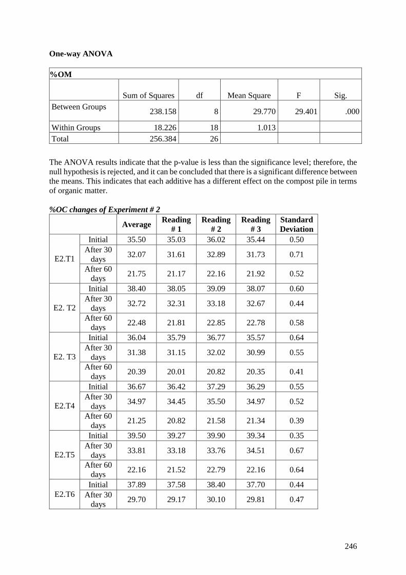
246
One-way ANOVA
%OM
Sum of Squares df Mean Square F Sig.
Between Groups 238.158 8 29.770 29.401 .000
Within Groups 18.226 18 1.013
Total 256.384 26
The ANOVA results indicate that the p-value is less than the significance level; therefore, the
null hypothesis is rejected, and it can be concluded that there is a significant difference between
the means. This indicates that each additive has a different effect on the compost pile in terms
of organic matter.
%OC changes of Experiment # 2
Average Reading
# 1
Reading
# 2
Reading
# 3
Standard
Deviation
E2.T1
Initial 35.50 35.03 36.02 35.44 0.50
After 30
days 32.07 31.61 32.89 31.73 0.71
After 60
days 21.75 21.17 22.16 21.92 0.52
E2. T2
Initial 38.40 38.05 39.09 38.07 0.60
After 30
days 32.72 32.31 33.18 32.67 0.44
After 60
days 22.48 21.81 22.85 22.78 0.58
E2. T3
Initial 36.04 35.79 36.77 35.57 0.64
After 30
days 31.38 31.15 32.02 30.99 0.55
After 60
days 20.39 20.01 20.82 20.35 0.41
E2.T4
Initial 36.67 36.42 37.29 36.29 0.55
After 30
days 34.97 34.45 35.50 34.97 0.52
After 60
days 21.25 20.82 21.58 21.34 0.39
E2.T5
Initial 39.50 39.27 39.90 39.34 0.35
After 30
days 33.81 33.18 33.76 34.51 0.67
After 60
days 22.16 21.52 22.79 22.16 0.64
E2.T6
Initial 37.89 37.58 38.40 37.70 0.44
After 30
days 29.70 29.17 30.10 29.81 0.47
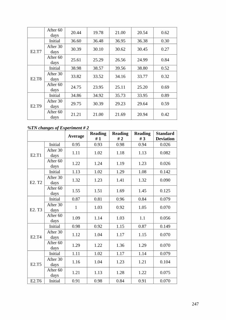
247
After 60
days 20.44 19.78 21.00 20.54 0.62
E2.T7
Initial 36.60 36.48 36.95 36.38 0.30
After 30
days 30.39 30.10 30.62 30.45 0.27
After 60
days 25.61 25.29 26.56 24.99 0.84
E2.T8
Initial 38.98 38.57 39.56 38.80 0.52
After 30
days 33.82 33.52 34.16 33.77 0.32
After 60
days 24.75 23.95 25.11 25.20 0.69
E2.T9
Initial 34.86 34.92 35.73 33.95 0.89
After 30
days 29.75 30.39 29.23 29.64 0.59
After 60
days 21.21 21.00 21.69 20.94 0.42
%TN changes of Experiment # 2
Average Reading
# 1
Reading
# 2
Reading
# 3
Standard
Deviation
E2.T1
Initial 0.95 0.93 0.98 0.94 0.026
After 30
days 1.11 1.02 1.18 1.13 0.082
After 60
days 1.22 1.24 1.19 1.23 0.026
E2. T2
Initial 1.13 1.02 1.29 1.08 0.142
After 30
days 1.32 1.23 1.41 1.32 0.090
After 60
days 1.55 1.51 1.69 1.45 0.125
E2. T3
Initial 0.87 0.81 0.96 0.84 0.079
After 30
days 1 1.03 0.92 1.05 0.070
After 60
days 1.09 1.14 1.03 1.1 0.056
E2.T4
Initial 0.98 0.92 1.15 0.87 0.149
After 30
days 1.12 1.04 1.17 1.15 0.070
After 60
days 1.29 1.22 1.36 1.29 0.070
E2.T5
Initial 1.11 1.02 1.17 1.14 0.079
After 30
days 1.16 1.04 1.23 1.21 0.104
After 60
days 1.21 1.13 1.28 1.22 0.075
E2.T6 Initial 0.91 0.98 0.84 0.91 0.070
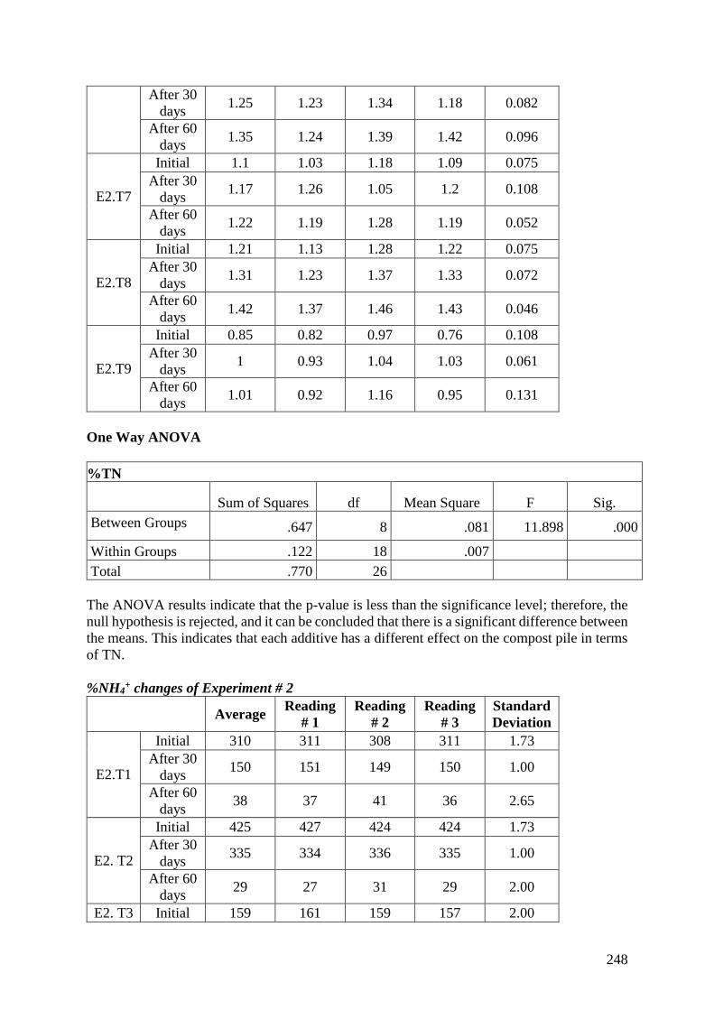
248
After 30
days 1.25 1.23 1.34 1.18 0.082
After 60
days 1.35 1.24 1.39 1.42 0.096
E2.T7
Initial 1.1 1.03 1.18 1.09 0.075
After 30
days 1.17 1.26 1.05 1.2 0.108
After 60
days 1.22 1.19 1.28 1.19 0.052
E2.T8
Initial 1.21 1.13 1.28 1.22 0.075
After 30
days 1.31 1.23 1.37 1.33 0.072
After 60
days 1.42 1.37 1.46 1.43 0.046
E2.T9
Initial 0.85 0.82 0.97 0.76 0.108
After 30
days 1 0.93 1.04 1.03 0.061
After 60
days 1.01 0.92 1.16 0.95 0.131
One Way ANOVA
%TN
Sum of Squares df Mean Square F Sig.
Between Groups .647 8 .081 11.898 .000
Within Groups .122 18 .007
Total .770 26
The ANOVA results indicate that the p-value is less than the significance level; therefore, the
null hypothesis is rejected, and it can be concluded that there is a significant difference between
the means. This indicates that each additive has a different effect on the compost pile in terms
of TN.
%NH4+ changes of Experiment # 2
Average Reading
# 1
Reading
# 2
Reading
# 3
Standard
Deviation
E2.T1
Initial 310 311 308 311 1.73
After 30
days 150 151 149 150 1.00
After 60
days 38 37 41 36 2.65
E2. T2
Initial 425 427 424 424 1.73
After 30
days 335 334 336 335 1.00
After 60
days 29 27 31 29 2.00
E2. T3 Initial 159 161 159 157 2.00
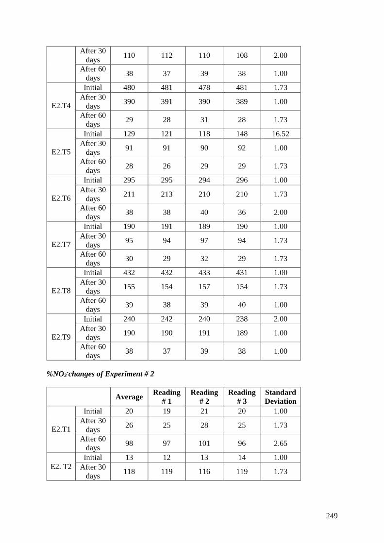
249
After 30
days 110 112 110 108 2.00
After 60
days 38 37 39 38 1.00
E2.T4
Initial 480 481 478 481 1.73
After 30
days 390 391 390 389 1.00
After 60
days 29 28 31 28 1.73
E2.T5
Initial 129 121 118 148 16.52
After 30
days 91 91 90 92 1.00
After 60
days 28 26 29 29 1.73
E2.T6
Initial 295 295 294 296 1.00
After 30
days 211 213 210 210 1.73
After 60
days 38 38 40 36 2.00
E2.T7
Initial 190 191 189 190 1.00
After 30
days 95 94 97 94 1.73
After 60
days 30 29 32 29 1.73
E2.T8
Initial 432 432 433 431 1.00
After 30
days 155 154 157 154 1.73
After 60
days 39 38 39 40 1.00
E2.T9
Initial 240 242 240 238 2.00
After 30
days 190 190 191 189 1.00
After 60
days 38 37 39 38 1.00
%NO3-changes of Experiment # 2
Average Reading
# 1
Reading
# 2
Reading
# 3
Standard
Deviation
E2.T1
Initial 20 19 21 20 1.00
After 30
days 26 25 28 25 1.73
After 60
days 98 97 101 96 2.65
E2. T2
Initial 13 12 13 14 1.00
After 30
days 118 119 116 119 1.73
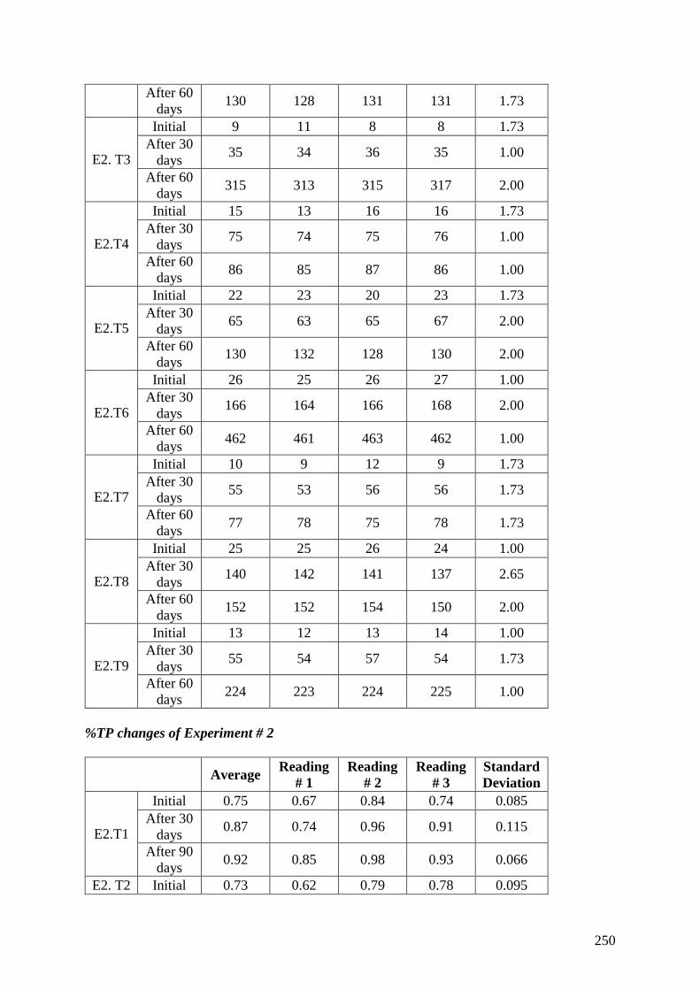
250
After 60
days 130 128 131 131 1.73
E2. T3
Initial 9 11 8 8 1.73
After 30
days 35 34 36 35 1.00
After 60
days 315 313 315 317 2.00
E2.T4
Initial 15 13 16 16 1.73
After 30
days 75 74 75 76 1.00
After 60
days 86 85 87 86 1.00
E2.T5
Initial 22 23 20 23 1.73
After 30
days 65 63 65 67 2.00
After 60
days 130 132 128 130 2.00
E2.T6
Initial 26 25 26 27 1.00
After 30
days 166 164 166 168 2.00
After 60
days 462 461 463 462 1.00
E2.T7
Initial 10 9 12 9 1.73
After 30
days 55 53 56 56 1.73
After 60
days 77 78 75 78 1.73
E2.T8
Initial 25 25 26 24 1.00
After 30
days 140 142 141 137 2.65
After 60
days 152 152 154 150 2.00
E2.T9
Initial 13 12 13 14 1.00
After 30
days 55 54 57 54 1.73
After 60
days 224 223 224 225 1.00
%TP changes of Experiment # 2
Average Reading
# 1
Reading
# 2
Reading
# 3
Standard
Deviation
E2.T1
Initial 0.75 0.67 0.84 0.74 0.085
After 30
days 0.87 0.74 0.96 0.91 0.115
After 90
days 0.92 0.85 0.98 0.93 0.066
E2. T2 Initial 0.73 0.62 0.79 0.78 0.095
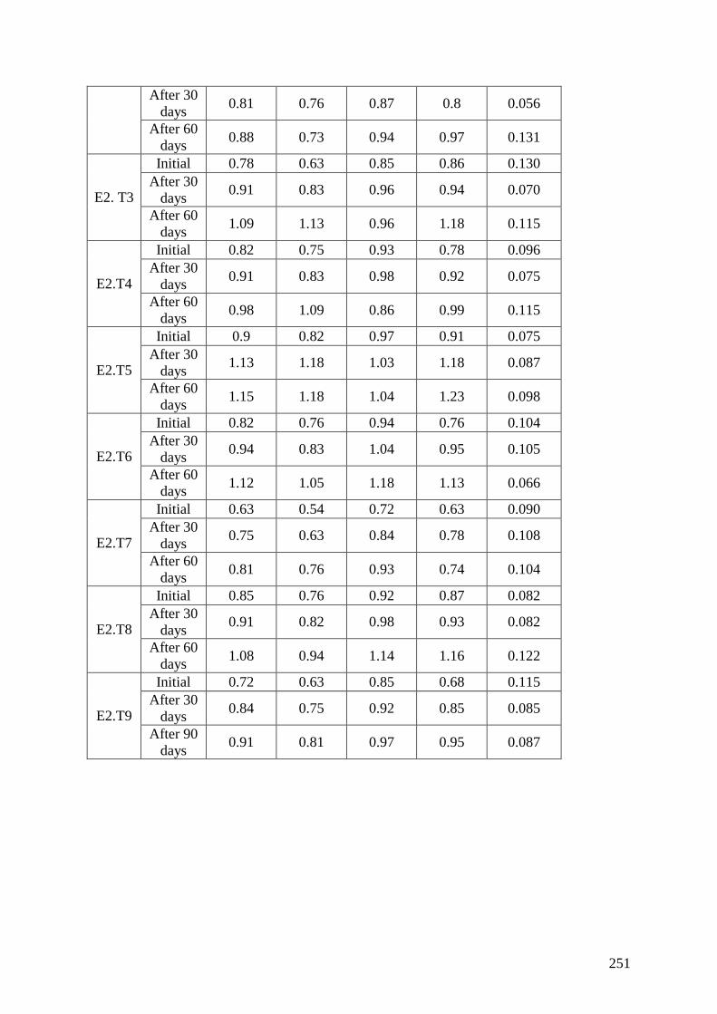
251
After 30
days 0.81 0.76 0.87 0.8 0.056
After 60
days 0.88 0.73 0.94 0.97 0.131
E2. T3
Initial 0.78 0.63 0.85 0.86 0.130
After 30
days 0.91 0.83 0.96 0.94 0.070
After 60
days 1.09 1.13 0.96 1.18 0.115
E2.T4
Initial 0.82 0.75 0.93 0.78 0.096
After 30
days 0.91 0.83 0.98 0.92 0.075
After 60
days 0.98 1.09 0.86 0.99 0.115
E2.T5
Initial 0.9 0.82 0.97 0.91 0.075
After 30
days 1.13 1.18 1.03 1.18 0.087
After 60
days 1.15 1.18 1.04 1.23 0.098
E2.T6
Initial 0.82 0.76 0.94 0.76 0.104
After 30
days 0.94 0.83 1.04 0.95 0.105
After 60
days 1.12 1.05 1.18 1.13 0.066
E2.T7
Initial 0.63 0.54 0.72 0.63 0.090
After 30
days 0.75 0.63 0.84 0.78 0.108
After 60
days 0.81 0.76 0.93 0.74 0.104
E2.T8
Initial 0.85 0.76 0.92 0.87 0.082
After 30
days 0.91 0.82 0.98 0.93 0.082
After 60
days 1.08 0.94 1.14 1.16 0.122
E2.T9
Initial 0.72 0.63 0.85 0.68 0.115
After 30
days 0.84 0.75 0.92 0.85 0.085
After 90
days 0.91 0.81 0.97 0.95 0.087
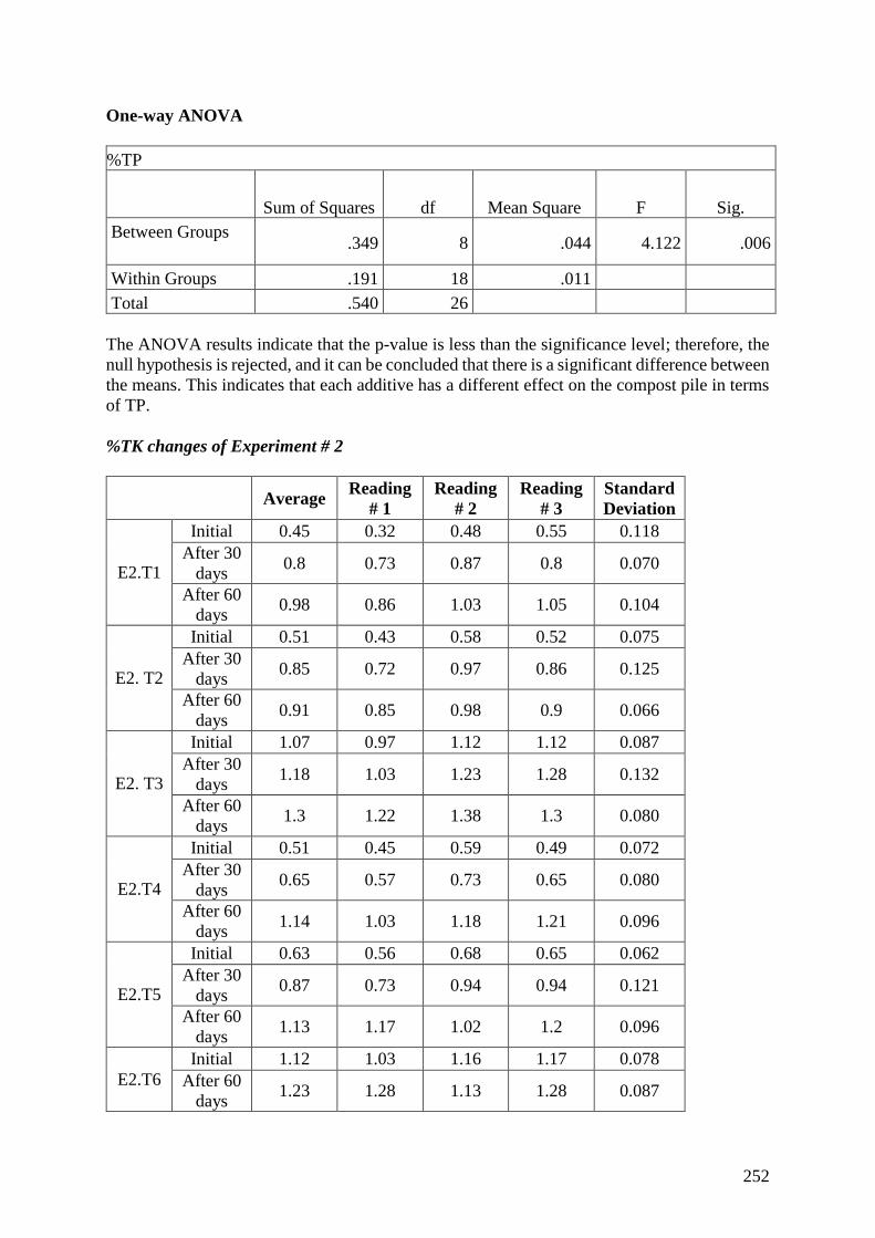
252
One-way ANOVA
%TP
Sum of Squares df Mean Square F Sig.
Between Groups .349 8 .044 4.122 .006
Within Groups .191 18 .011
Total .540 26
The ANOVA results indicate that the p-value is less than the significance level; therefore, the
null hypothesis is rejected, and it can be concluded that there is a significant difference between
the means. This indicates that each additive has a different effect on the compost pile in terms
of TP.
%TK changes of Experiment # 2
Average Reading
# 1
Reading
# 2
Reading
# 3
Standard
Deviation
E2.T1
Initial 0.45 0.32 0.48 0.55 0.118
After 30
days 0.8 0.73 0.87 0.8 0.070
After 60
days 0.98 0.86 1.03 1.05 0.104
E2. T2
Initial 0.51 0.43 0.58 0.52 0.075
After 30
days 0.85 0.72 0.97 0.86 0.125
After 60
days 0.91 0.85 0.98 0.9 0.066
E2. T3
Initial 1.07 0.97 1.12 1.12 0.087
After 30
days 1.18 1.03 1.23 1.28 0.132
After 60
days 1.3 1.22 1.38 1.3 0.080
E2.T4
Initial 0.51 0.45 0.59 0.49 0.072
After 30
days 0.65 0.57 0.73 0.65 0.080
After 60
days 1.14 1.03 1.18 1.21 0.096
E2.T5
Initial 0.63 0.56 0.68 0.65 0.062
After 30
days 0.87 0.73 0.94 0.94 0.121
After 60
days 1.13 1.17 1.02 1.2 0.096
E2.T6
Initial 1.12 1.03 1.16 1.17 0.078
After 60
days 1.23 1.28 1.13 1.28 0.087
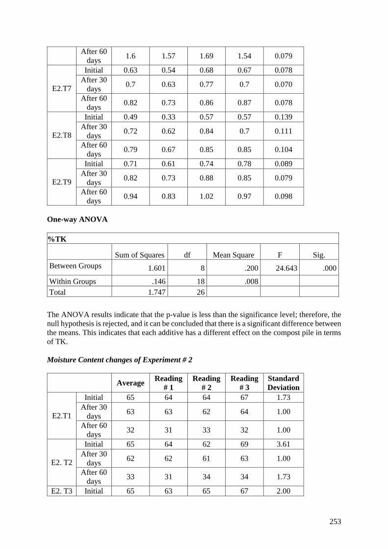
253
After 60
days 1.6 1.57 1.69 1.54 0.079
E2.T7
Initial 0.63 0.54 0.68 0.67 0.078
After 30
days 0.7 0.63 0.77 0.7 0.070
After 60
days 0.82 0.73 0.86 0.87 0.078
E2.T8
Initial 0.49 0.33 0.57 0.57 0.139
After 30
days 0.72 0.62 0.84 0.7 0.111
After 60
days 0.79 0.67 0.85 0.85 0.104
E2.T9
Initial 0.71 0.61 0.74 0.78 0.089
After 30
days 0.82 0.73 0.88 0.85 0.079
After 60
days 0.94 0.83 1.02 0.97 0.098
One-way ANOVA
%TK
Sum of Squares df Mean Square F Sig.
Between Groups 1.601 8 .200 24.643 .000
Within Groups .146 18 .008
Total 1.747 26
The ANOVA results indicate that the p-value is less than the significance level; therefore, the
null hypothesis is rejected, and it can be concluded that there is a significant difference between
the means. This indicates that each additive has a different effect on the compost pile in terms
of TK.
Moisture Content changes of Experiment # 2
Average Reading
# 1
Reading
# 2
Reading
# 3
Standard
Deviation
E2.T1
Initial 65 64 64 67 1.73
After 30
days 63 63 62 64 1.00
After 60
days 32 31 33 32 1.00
E2. T2
Initial 65 64 62 69 3.61
After 30
days 62 62 61 63 1.00
After 60
days 33 31 34 34 1.73
E2. T3 Initial 65 63 65 67 2.00
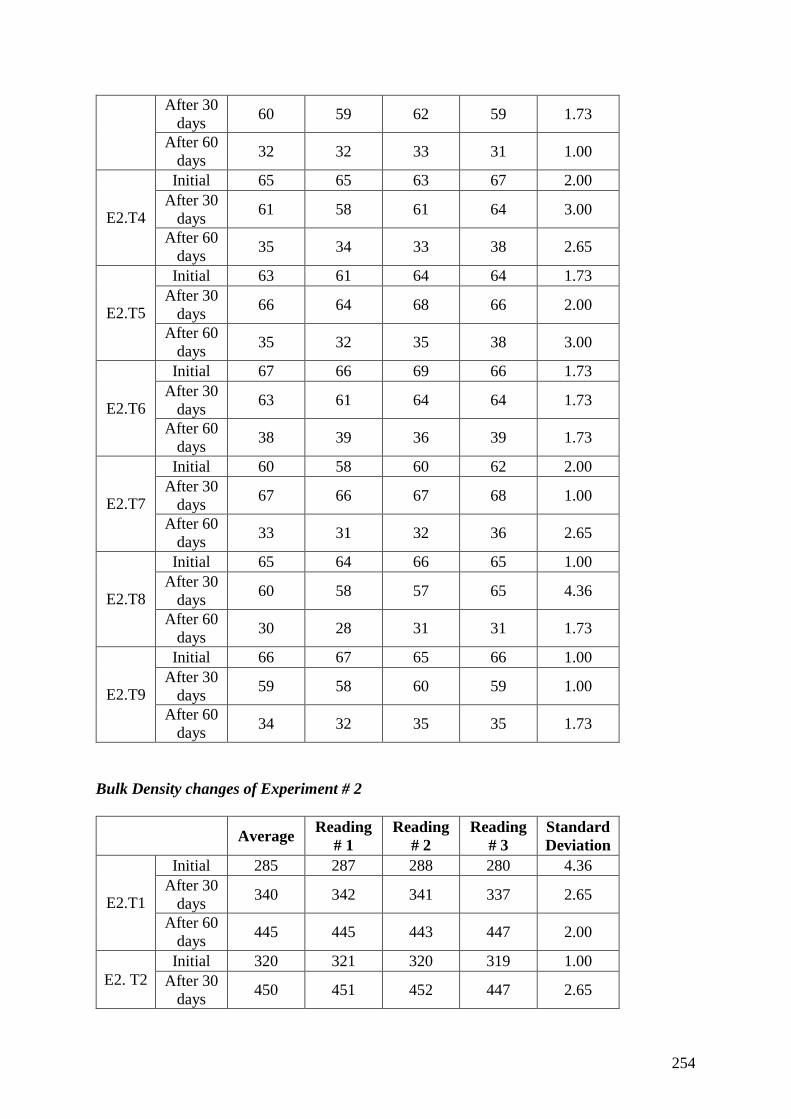
254
After 30
days 60 59 62 59 1.73
After 60
days 32 32 33 31 1.00
E2.T4
Initial 65 65 63 67 2.00
After 30
days 61 58 61 64 3.00
After 60
days 35 34 33 38 2.65
E2.T5
Initial 63 61 64 64 1.73
After 30
days 66 64 68 66 2.00
After 60
days 35 32 35 38 3.00
E2.T6
Initial 67 66 69 66 1.73
After 30
days 63 61 64 64 1.73
After 60
days 38 39 36 39 1.73
E2.T7
Initial 60 58 60 62 2.00
After 30
days 67 66 67 68 1.00
After 60
days 33 31 32 36 2.65
E2.T8
Initial 65 64 66 65 1.00
After 30
days 60 58 57 65 4.36
After 60
days 30 28 31 31 1.73
E2.T9
Initial 66 67 65 66 1.00
After 30
days 59 58 60 59 1.00
After 60
days 34 32 35 35 1.73
Bulk Density changes of Experiment # 2
Average Reading
# 1
Reading
# 2
Reading
# 3
Standard
Deviation
E2.T1
Initial 285 287 288 280 4.36
After 30
days 340 342 341 337 2.65
After 60
days 445 445 443 447 2.00
E2. T2
Initial 320 321 320 319 1.00
After 30
days 450 451 452 447 2.65
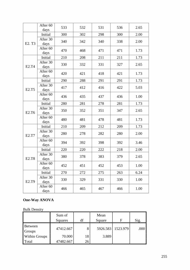
255
After 60
days 533 532 531 536 2.65
E2. T3
Initial 300 302 298 300 2.00
After 30
days 340 342 340 338 2.00
After 60
days 470 468 471 471 1.73
E2.T4
Initial 210 208 211 211 1.73
After 30
days 330 332 331 327 2.65
After 60
days 420 421 418 421 1.73
E2.T5
Initial 290 288 291 291 1.73
After 30
days 417 412 416 422 5.03
After 60
days 436 435 437 436 1.00
E2.T6
Initial 280 281 278 281 1.73
After 30
days 350 352 351 347 2.65
After 60
days 480 481 478 481 1.73
E2.T7
Initial 210 209 212 209 1.73
After 30
days 280 278 282 280 2.00
After 60
days 394 392 398 392 3.46
E2.T8
Initial 220 220 222 218 2.00
After 30
days 380 378 383 379 2.65
After 60
days 452 451 452 453 1.00
E2.T9
Initial 270 272 275 263 6.24
After 30
days 330 329 331 330 1.00
After 60
days 466 465 467 466 1.00
One-Way ANOVA
Bulk Density
Sum of
Squares df
Mean
Square F Sig.
Between
Groups 47412.667 8 5926.583 1523.979 .000
Within Groups 70.000 18 3.889
Total 47482.667 26
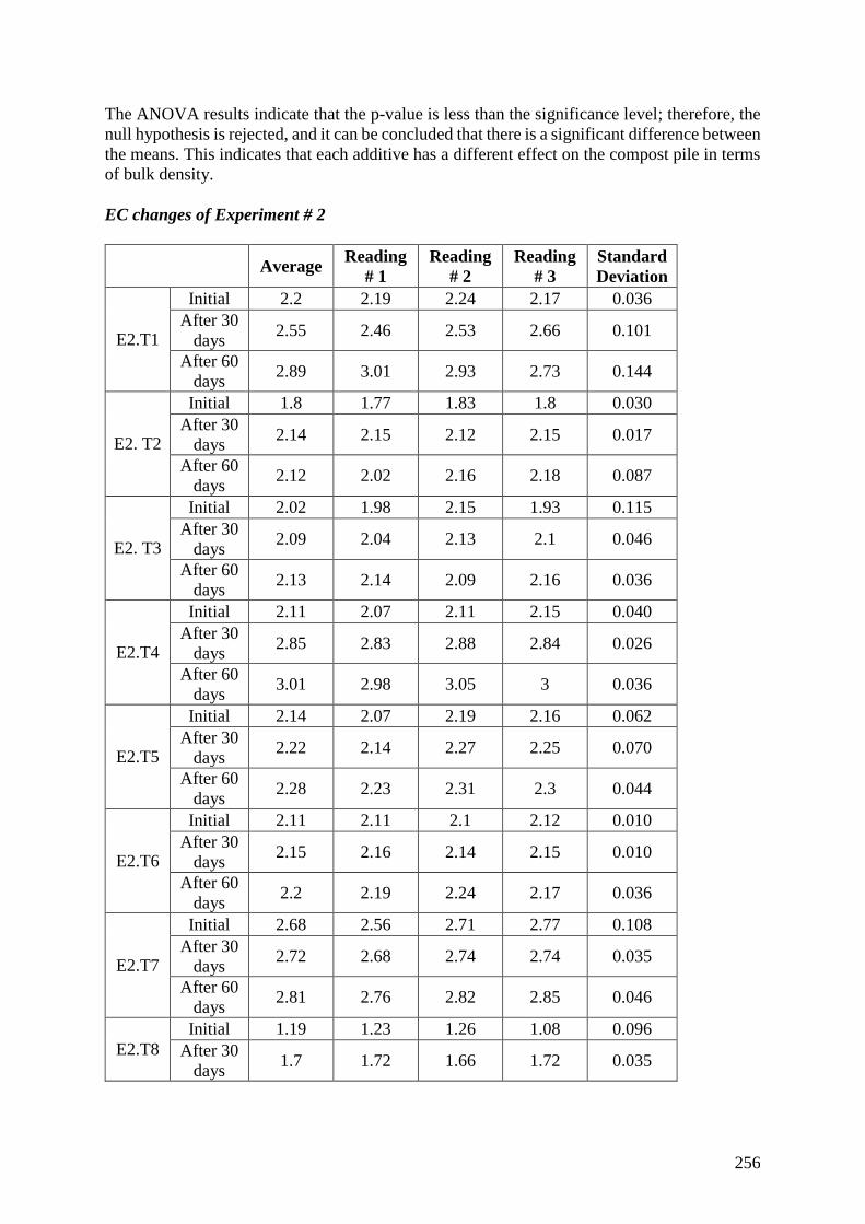
256
The ANOVA results indicate that the p-value is less than the significance level; therefore, the
null hypothesis is rejected, and it can be concluded that there is a significant difference between
the means. This indicates that each additive has a different effect on the compost pile in terms
of bulk density.
EC changes of Experiment # 2
Average Reading
# 1
Reading
# 2
Reading
# 3
Standard
Deviation
E2.T1
Initial 2.2 2.19 2.24 2.17 0.036
After 30
days 2.55 2.46 2.53 2.66 0.101
After 60
days 2.89 3.01 2.93 2.73 0.144
E2. T2
Initial 1.8 1.77 1.83 1.8 0.030
After 30
days 2.14 2.15 2.12 2.15 0.017
After 60
days 2.12 2.02 2.16 2.18 0.087
E2. T3
Initial 2.02 1.98 2.15 1.93 0.115
After 30
days 2.09 2.04 2.13 2.1 0.046
After 60
days 2.13 2.14 2.09 2.16 0.036
E2.T4
Initial 2.11 2.07 2.11 2.15 0.040
After 30
days 2.85 2.83 2.88 2.84 0.026
After 60
days 3.01 2.98 3.05 3 0.036
E2.T5
Initial 2.14 2.07 2.19 2.16 0.062
After 30
days 2.22 2.14 2.27 2.25 0.070
After 60
days 2.28 2.23 2.31 2.3 0.044
E2.T6
Initial 2.11 2.11 2.1 2.12 0.010
After 30
days 2.15 2.16 2.14 2.15 0.010
After 60
days 2.2 2.19 2.24 2.17 0.036
E2.T7
Initial 2.68 2.56 2.71 2.77 0.108
After 30
days 2.72 2.68 2.74 2.74 0.035
After 60
days 2.81 2.76 2.82 2.85 0.046
E2.T8
Initial 1.19 1.23 1.26 1.08 0.096
After 30
days 1.7 1.72 1.66 1.72 0.035
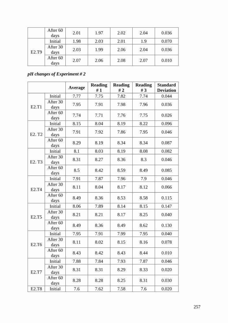
257
After 60
days 2.01 1.97 2.02 2.04 0.036
E2.T9
Initial 1.98 2.03 2.01 1.9 0.070
After 30
days 2.03 1.99 2.06 2.04 0.036
After 60
days 2.07 2.06 2.08 2.07 0.010
pH changes of Experiment # 2
Average Reading
# 1
Reading
# 2
Reading
# 3
Standard
Deviation
E2.T1
Initial 7.77 7.75 7.82 7.74 0.044
After 30
days 7.95 7.91 7.98 7.96 0.036
After 60
days 7.74 7.71 7.76 7.75 0.026
E2. T2
Initial 8.15 8.04 8.19 8.22 0.096
After 30
days 7.91 7.92 7.86 7.95 0.046
After 60
days 8.29 8.19 8.34 8.34 0.087
E2. T3
Initial 8.1 8.03 8.19 8.08 0.082
After 30
days 8.31 8.27 8.36 8.3 0.046
After 60
days 8.5 8.42 8.59 8.49 0.085
E2.T4
Initial 7.91 7.87 7.96 7.9 0.046
After 30
days 8.11 8.04 8.17 8.12 0.066
After 60
days 8.49 8.36 8.53 8.58 0.115
E2.T5
Initial 8.06 7.89 8.14 8.15 0.147
After 30
days 8.21 8.21 8.17 8.25 0.040
After 60
days 8.49 8.36 8.49 8.62 0.130
E2.T6
Initial 7.95 7.91 7.99 7.95 0.040
After 30
days 8.11 8.02 8.15 8.16 0.078
After 60
days 8.43 8.42 8.43 8.44 0.010
E2.T7
Initial 7.88 7.84 7.93 7.87 0.046
After 30
days 8.31 8.31 8.29 8.33 0.020
After 60
days 8.28 8.28 8.25 8.31 0.030
E2.T8 Initial 7.6 7.62 7.58 7.6 0.020

258
After 30
days 8.29 8.31 8.25 8.31 0.035
After 60
days 8.12 8.11 8.16 8.09 0.036
E2.T9
Initial 7.65 7.62 7.67 7.66 0.026
After 30
days 8.4 8.41 8.37 8.42 0.026
After 60
days 8.69 8.67 8.73 8.67 0.035