Embed Size (px)
Citation preview
Manuscript prepared for Clim. Pastwith version 4.2 of the LATEX class copernicus.cls.Date: 26 September 2012
HadISD: A quality controlled global synoptic report database forselected variables at long-term stations from 1973-2011R. J. H. Dunn1, K. M. Willett1, P. W. Thorne2, E. V. Woolley2, I. Durre4, A. Dai5, D. E. Parker1, and R. S. Vose4
1Met Office Hadley Centre, FitzRoy Road, Exeter, EX1 3PB, UK2Cooperative Institute for Climate and Satellites, North Carolina State University and NOAAs National Climatic Data Center,Patton Avenue, Asheville, NC, 28801, USA3Formerly at: Met Office Hadley Centre, FitzRoy Road, Exeter, EX1 3PB, UK4NOAAs National Climatic Data Center, Patton Avenue, Asheville, NC, 28801, USA5National Center for Atmospheric Research (NCAR), P. O. 3000, Boulder, CO 80307, USA
Abstract. This paper describes the creation of HadISD; anautomatically quality-controlled synoptic resolution datasetof temperature, dewpoint temperature, sea-level pressure,wind speed, wind direction and cloud cover from globalweather stations for 1973-2011. The full dataset consistsof over 6,000 stations, with 3427 long-term stations deemedto have sufficient sampling and quality for climate appli-cations requiring sub-daily resolution. As with other sur-face datasets, coverage is heavily skewed towards NorthernHemisphere mid-latitudes.
The dataset is constructed from a large pre-existing ASCIIflatfile data-bank that represents over a decade of substan-tial effort at data retrieval, reformatting and provision. Theseraw data have had varying levels of quality control appliedto them by individual data providers. The work proceeded inseveral steps: merging stations with multiple reporting iden-tifiers; reformatting to netcdf; quality control; and then filter-ing to form a final dataset. Particular attention has been paidto maintaining true extreme values where possible within anautomated, objective process. Detailed validation has beenperformed on a subset of global stations and also on UK datausing known extreme events to help finalise the QC tests.Further validation was performed on a selection of extremeevents world-wide (Hurricane Katrina in 2005, the cold snapin Alaska in 1989 and heat waves in SE Australia in 2009).Some very initial analyses are performed to illustrate someof the types of problems to which the final data could be ap-plied. Although the filtering has removed the poorest stationrecords, no attempt has been made to homogenise the datathus far, due to the complexity of retaining the true distri-bution of high-resolution data when applying adjustments.Hence non-climatic, time-varying errors may still exist inmany of the individual station records and care is needed ininferring long-term trends from these data.
This dataset will allow the study of high frequency varia-
Correspondence to: [email protected]
tions of temperature, pressure and humidity on a global basisover the last four decades. Both individual extremes and theoverall population of extreme events could be investigated indetail to allow for comparison with past and projected cli-mate. A version-control system has been constructed for thisdataset to allow for the clear documentation of any updatesand corrections in the future.
1 Introduction
The Integrated Surface Database (ISD) held at NOAAsNational Climatic Data Center is an archive of syn-optic reports from a large number of global sur-face stations (Smith et al., 2011; Lott, 2004 seehttp://www.ncdc.noaa.gov/oa/climate/isd/index.php). Itis a rich source of data useful for the study of climatevariations, individual meteorological events and historicalclimate impacts. For example, these data have been appliedto quantify precipitation frequency (Dai, 2001a) and itsdiurnal cycle (Dai, 2001b), diurnal variations in surfacewinds and divergence field (Dai and Deser, 1999), and recentchanges in surface humidity (Dai, 2006; Willett et al., 2008),cloudiness (Dai et al., 2006)) and wind speed (Peterson etal., 2011).
The collation of ISD, merging and reformatting to a singleformat from over 100 constituent sources and three majordatabanks represented a substantial and ground-breaking ef-fort undertaken over more than a decade at NOAA NCDC.The database is updated in near real-time. A number of auto-mated quality control (QC) tests are applied to the data thatlargely consider internal station series consistency and aregeographically invariant in their application (i.e. thresholdvalues are the same for all stations regardless of the local cli-matology). These procedures are briefly outlined in (Lott,2004) and (Smith et al., 2011). The tests concentrate onthe most widely used variables and consist of a mix of log-
2 R. J. H. Dunn et al.: HadISD: a quality-controlled global synoptic database
ical consistency checks and outlier type checks. Values areflagged rather than deleted. Automated checks are essentialas it is impractical to manually check thousands of individ-ual station records that could each consist of several tens ofthousands of individual observations. It should be noted thatthe raw data in many cases have been previously quality con-trolled manually by the data providers, so the raw data arenot necessarily completely raw for all stations.
The ISD database is non-trivial for the non-expert toaccess and use, as each station consists of a series ofannual ASCII flatfiles (with each year being a sepa-rate directory) with each observation representing a rowin a format akin to the synoptic reporting codes thatis not immediately intuitive or amenable to easy ma-chine reading (http://www1.ncdc.noaa.gov/pub/data/ish/ish-format-document.pdf). NCDC, however, provides access tothe ISD database using a GIS interface. This does give theability for users to select parameters and stations and out-put the results to a text file. Also, a subset of the ISD vari-ables (air temperature, dewpoint temperature, sea level pres-sure, wind direction, wind speed, total cloud cover, one-houraccumulated liquid precipitation, six-hour accumulated liq-uid precipitation) is available as ISD-Lite in fixed-width for-mat ASCII files. However, there has been no selection ondata or station quality. In this paper we outline the steps un-dertaken to provide a new quality controlled version, calledHadISD, which is based on the raw ISD records, in netcdfformat for selected variables for a subset of the stations withlong records. This new dataset will allow the easy study ofthe behaviour of short-timescale climate phenomena in re-cent decades, with the subsequent comparison to past cli-mates and future climate projections.
One of the primary uses of a sub-daily resolution databasewill be the characterisation of extreme events for specific lo-cations, and so it is imperative that multiple, independent ef-forts be undertaken to assess the fundamental quality of in-dividual observations. We also therefore undertake a newand comprehensive quality control of the ISD, based uponthe raw holdings, which should be seen as complimentaryto that which already exists. In the same way that multi-ple independent homogenisation efforts have informed ourunderstanding of true long-term trends in variables such astropospheric temperatures (Thorne et al., 2011), numerousindependent QC efforts will be required to fully understandchanges in extremes. Arguably, in this context structural un-certainty (Thorne et al., 2005) in quality control choices willbe as important as that in any homogenisation processes thatwere to be applied in ensuring an adequate portrayal of ourtrue degree of uncertainty in extremes behaviour. Poorly ap-plied quality control processes could certainly have a moredetrimental effect than poor homogenisation processes. Tooaggressive and the real tails are removed, too liberal and dataartefacts remain to be mis-interpreted by the unwary. As weare unable to know for certain whether a given value is trulyvalid, it is impossible to unambiguously determine the preva-
lence of type-I and type-II errors for any candidate QC algo-rithm. In this work, type-I errors occur when a good valueis flagged, and type-II errors are when a bad value is notflagged.
Quality control is therefore an increasingly important as-pect of climate dataset construction as the focus moves to-wards regional and local scale impacts and mitigation in sup-port of climate services (Doherty et al., 2008). The data re-quired to support these applications need to be at a much finertemporal and spatial resolution than is typically the case formost climate datasets, free of gross errors and homogenisedin such a way as to retain the high as well as low temporal fre-quency characteristics of the record. Homogenisation at theindividual observation level is a separate and arguably sub-stantially more complex challenge. Here we describe solelythe data preparation and QC. The methodology is looselybased upon that developed in (Durre et al., 2010) for dailydata from the Global Historical Climatology Network. Fur-ther discussion of the data QC problem, previous efforts andreferences can be found therein. These historical issues arenot covered in any detail here.
Section 2 describes how stations that report under varyingidentifiers were combined an issue that was found to be glob-ally insidious and particularly prevalent in certain regions.Section 3 outlines selection of an initial set of stations forsubsequent QC. Section 4 outlines the intra- and inter-stationQC procedures developed and summarises their impact. Wevalidate the final quality controlled dataset in Section 5. Sec-tion 6 briefly summarises the final selection of stations andSection 7 describes our version numbering system. Section8 outlines some very simple analyses of the data to illustratetheir likely utility, whilst Section 9 concludes.
The final data are available throughhttp://www.metoffice.gov.uk/hadobs/hadisd along withthe large volume of process metadata that cannot reasonablybe appended to this paper. The database covers 1973 toend-2011, because availability drops off substantially priorto 1973 (Willett et al., 2008). In future periodic updates areplanned to keep the dataset up to date.
2 Compositing Stations
The ISD database archives according to the station identi-fier (ID) appended to the report transmission, resulting inaround 28,000 individual station IDs. Despite efforts by theISD dataset creators, this causes issues for stations that havechanged their reporting ID frequently or that have reportedsimultaneously under multiple IDs to different ISD sourcedatabanks (i.e. using a WMO identifier over the GTS and anational identifier to a local repository). Many such stationsrecords exist in multiple independent station files within theISD database despite in reality being a single station record.In some regions, e.g. Canada and parts of Eastern Europe,

R. J. H. Dunn et al.: HadISD: a quality-controlled global synoptic database 3
WMO station ID changes have been ubiquitous, so composit-ing is essential for record completeness.
Station location and ID information were read from theISD station inventory, and the potential for station matchesassessed by pairwise comparisons using a hierarchical scor-ing system (Table 1). The inventory is used instead of withindata file location information as the latter had been found tobe substantially more questionable (Neal Lott, pers. comm.).Scores are high for those elements which, if identical, wouldgive high confidence that the stations are the same. For ex-ample it is highly implausible that a METAR call sign willhave been recycled between geographically distinct stations.Station pairs that exceeded a total score of 14 are selected forfurther analysis (see Table 1). So a candidate pair for con-sideration must at an absolute minimum be: close in distanceand elevation and from the same country, or have the same IDor name. Several stations appeared in more than one uniquepairing of potential composites. These cases were combinedto form consolidated sets of potential matches. Some of thesesets comprise as many as five apparently unique station IDsin the ISD database.
For each potential station match set, in additionto the hierarchical scoring system value (Table 1),were considered graphically the following quantities:00UTC temperature anomalies from the ISD-lite database[http://www.ncdc.noaa.gov/oa/climate/isd/index.php] usinganomalies relative to the mean of the entire set of candidatestation records; the ISD-lite data count by month; and thedaily distribution of observing times. This required in-depthmanual input taking roughly a calendar month to completeresulting in 1,504 likely composite sets assigned as matches(comprising 3353 unique station IDs, Figure 1). Of thesejust over half are very obviously the same station. For exam-ple: data ceased from one identifier simultaneously with datacommencing from the other where the data are clearly notsubstantially inhomogeneous across the break; or the differ-ent identifiers report at different synoptic hours but all otherdetails are the same. Other cases were less clear, in mostcases because data overlap implied potentially distinct sta-tions or discontinuities yielding larger uncertainties in as-signment. Assigned sets were merged giving initial prefer-ence to longer record segments but allowing infilling of miss-ing elements where records overlap from the shorter segmentrecords to maximise record completeness. This matching ofstations was carried out on an earlier extraction of the ISDdataset spanning 1973 to 2007. The final dataset is based onan extraction from the ISD of data spanning 1973 to end-2011, and the station assignments have been carried overwith no reanalysis.
There may well be assigned composites that should beseparate stations, especially in densely sampled regions ofthe globe. If the merge were being done for the raw ISDarchive that constitutes the baseline synoptic dataset heldin the designated WMO World Data Centre, then far moremeticulous analysis would be required. For this value added
product a few false station merges can be tolerated and lateramended/removed if detected. The station IDs that werecombined to form a single record are noted in the metadataof the final output file where appropriate. A list of the iden-tifiers of the 943 stations in the final dataset which are as-signed composites as well as their component station IDs canbe found on the HadISD website.
3 Selection and Retrieval of an initial set of stations
The ISD consists of a large number of stations some of whichhave reported only rarely. Of the 30,000 stations, about 2/3have observations in 30 years or fewer and several thousandhave small total file sizes, corresponding to few observations.However, almost 2000 stations have long records extend-ing 60 or more years between 1901 and end-2011. Most ofthese have large total file sizes indicating quasi-continuousrecords, rather than only a few observations per year. Tosimplify selection, only stations which may plausibly haverecords suitable for climate applications were considered, us-ing two key requirements: length of record and reporting fre-quency. The latter is important for characterisation of ex-tremes, as too infrequent observing will greatly reduce thepotential to capture both truly extreme events and the diurnalcycle characteristics. A degree of pre-screening was there-fore deemed necessary prior to application of QC tests towinnow out those records which would be grossly inappro-priate for climate studies.
To maximise spatial coverage, network distributions forfour climatology periods (1976-2005, 1981-2000, 1986-2005 and 1991-2000) and four different average time stepsbetween consecutive reports (hourly, 3-hourly, 6-hourly, 12-hourly) were compared. For a station to qualify for a clima-tology period, at least half of the years within the climatol-ogy period must have a corresponding data file regardless ofits size. No attempt was made at this very initial screeningstage to ensure these are well distributed within the clima-tological period. To assign the reporting frequency, (up to)the first 250 observations of each annual file were used towork out the average interval between consecutive observa-tions. With hourly frequency stipulation coverage collapsesto essentially NW Europe and N. America (Figure 2). Threehourly frequency yields a much more globally complete dis-tribution. There is little additional coverage or station densityderived by further coarsening to 6 (not shown) or 12 hourlyexcept in parts of Australia, S. America and the Pacific. Sen-sitivity to choice of climatology period is much smaller (notshown) so a 1976-2005 climatology period and a 3 hourlyreporting frequency were chosen as a minimum requirement.This selection resulted in 6187 stations selected for furtheranalysis.
ISD raw data files are (potentially) very large ASCII flatfiles – one per station per year. The stations data were con-verted to hourly resolution netcdf files for a subset of the vari-
4 R. J. H. Dunn et al.: HadISD: a quality-controlled global synoptic database
ables including both WMO-designated mandatory and op-tional reporting parameters. Details of all variables retrievedand those considered further in the current quality controlsuite are given in Table 2. There are some stations which forpart of the analysed period report at sub hourly frequencies.As both temperature and dewpoint temperature are requiredto be measured simultaneously for any study on humidity tobe reliably carried out, reports which have both temperatureand dewpoint temperature observations are favoured (underthe assumption that the readings were taken at close proxim-ity in space and time) over those reports which have one orthe other (but not both), even if the reports with both obser-vations are further from the full hour. In cases where obser-vations only have temperature or dewpoint temperature (andnever both), then those with temperature are favoured, evenif these are further from the full hour (00 minutes). All vari-ables in a single HadISD hourly time step always derive froma single ISD time step, with no blending between the variouswithin-hour reports. However the HadISD times are alwaysconverted to the nearest whole hour. To minimise data stor-age the time axis is collapsed in the netcdf files so that onlytime steps with observations are retained.
4 Quality control steps and analysis
An individual hourly station record with full temporal sam-pling from 1973 to 2011 could contain in excess of 340,000observations and there are>6,000 candidate stations. Hence,a fully-automated quality-control procedure was essential. Asimilar approach to that of GHCND (Durre et al., 2010) wastaken. Intra-station tests were initially trained against a sin-gle (UK) case-study station series with bad data deliberatelyintroduced to ensure that the tests, at least to first order, be-haved as expected. Both intra- and inter-station tests werethen further designed, developed and validated based uponexpert judgment and analysis using a set of 76 stations fromacross the Globe (listed on the HadISD website). This set in-cluded both stations with proportionally large data removalsin early versions of the tests and GCOS (Global ClimateObserving System) Surface Network stations known to behighly equipped and well staffed so that major problems areunlikely. The test software suite took a number of iterationsto obtain a satisfactorily small expert judgement false pos-itive rate (type I error rate) and, on subjective assessment,a clean dataset for these stations. In addition, geographicalmaps of detection rates were viewed for each test and in to-tal to ensure that rejection rates did not appear to have a realphysical basis for any given test or variable. Deeper valida-tion on UK stations (IDs beginning 03) was carried out usingthe well-documented 2003 heat wave and storms of 1987 and1990. This resulted in a further round of refining, resultingin the tests as presented below.
Wherever distributional assumptions were made, an indi-cator that is robust to outliers was required. Pervasive data
issues can lead to an unduly large standard deviation (σ) be-ing calculated which results in the tests being too conserva-tive. So, the inter-quartile range (IQR) or the median abso-lute deviation (MAD) were used instead; these sample solelythe (presumably reasonable) core portion of the distribution.The IQR samples 50 per cent of the population whereas±1σencapsulates 68 per cent of the population for a truly normaldistribution. One IQR is 1.35σ, and one MAD is 0.67σ if theunderlying data are truly normally distributed.
The Durre et al. (2010) method applies tests in a de-liberate order, removing bad data progressively. Here, aslightly different approach is taken including a multi-levelflagging system. All bad data have associated flags identi-fying the tests that they failed. Some tests result in instan-taneous data removal (latitude-longitude and station dupli-cate checks) whereas most just flag the data. Flagged, butretained, data are not used for any further derivations of testthresholds. However, all retained data undergo each test suchthat an individual observation may receive multiple flags.Furthermore, some of the tests outlined in the next section settentative flags. These values can be reinstated using compar-isons with neighbouring stations in a later test, which reducesthe chances of removing true local or regional extremes. Thetests are conducted in a specified order such that large chunksof bad data are removed from the test threshold derivationsfirst and so the tests become progressively more sensitive.After an initial latitude-longitude check (which removed onestation) and a duplicate station check, intra-station tests areapplied to the station in isolation, followed by inter-stationneighbour comparisons. A subset of the intra-station testsare then re-run, followed by the inter-station checks againand then a final clean up (Figure 3).
4.1 QC tests
4.1.1 Test 1. Inter-station duplicate check
It is possible that two unique station identifiers actually con-tain identical data. This may be simple data management er-ror or an artefact of dummy station files intended for tempo-rary data storage. To detect these, each stations temperaturetime series is compared iteratively with that of every otherstation. To account for reporting time (t) issues the series areoffset by 1 hour steps between t−11 and t+11 hours. Serieswith > 1000 coincident non-missing data points, of whichover 25 per cent are flagged as exact duplicates, are listedfor further consideration. This computer-intensive check re-sulted in 280 stations being put forward for manual scrutiny.
All duplicate pairs and groups were then manually as-sessed using the match statistics, reporting frequencies, sep-aration distance and time series of the stations involved. Ifa station pair had exact matches on ≥ 70 per cent of poten-tial occasions, then the shortest station of the pair was re-moved. This results in a further loss of stations. As this test issearching for duplicates after the merging of composite sta-
R. J. H. Dunn et al.: HadISD: a quality-controlled global synoptic database 5
tions (Section 2), any stations found by this test did not pre-viously meet the requirements for stations to be merged, butstill have significant periods where the observations are du-plicated. Therefore the removal of data is the safest course ofaction. Stations that appeared in the potential duplicates listtwice or more were also removed. A further subjective deci-sion was taken to remove any stations having a very patchyor obscure time series, for example with very high variance.This set of checks removed a total of 83 stations, (Figure 1),leaving 6103 to go forward into the rest of the QC procedure.
4.1.2 Test 2. Duplicate months check
Given day-to-day weather, an exact match of synoptic datafor a month with any other month in that station is highly un-likely. This test checks for exact replicas of whole months oftemperature data where at least 20 observations are present.Each month is pattern-matched for data presence with allother months, and any months with exact duplicates for eachmatched value are flagged. As it cannot be known a prioriwhich month is correct, both are flagged. Although the testwas successful at detecting deliberately engineered duplica-tion in a case study station no occurrences of such errors werefound within the real data. The test was retained for com-pleteness and also because such an error may occur in futureupdates of HadISD.
4.1.3 Test 3. Odd Cluster Check
A number of time series exhibit isolated clusters of data. Aninstrument that reports sporadically is of questionable scien-tific value. Furthermore, with little or no surrounding data itis much more difficult to determine whether individual ob-servations are valid. Hence, any short clusters of up to 6hours within a 24 hour period separated by 48 hours or longerfrom all other data are flagged. This applies to tempera-ture, dewpoint temperature and sea-level pressure elementsindividually. These flags can be undone if the neighbour-ing stations have concurrent, unflagged observations whoserange encompasses the observations in question (see Section4.1.14).
4.1.4 Test 4. Frequent value check
The problem of frequent values found in (Durre et al., 2010)also extends to synoptic data. Some stations contain far moreobservations of a given value than would be reasonably ex-pected. This could be the use of zero to signify missingdata, or the occurrence of some other local data-issue identi-fier1 that has been mistakenly ingested into the database as atrue value. This test identifies suspect values using the entire
1A “local data-issue identifier” is where a physically valid butlocally implausible value is used to mark a problem with a particulardata point. On subsequent ingestion into the ISD, this value hasbeen interpreted as a real measurement rather than a flag.
record and then scans for each value on a year-by-year basisto flag only if they are a problem within that year.
This test is also run seasonally (JF+D, MAM, JJA, SON),using a similar approach as above. Each set of three monthsare scanned over the entire record to identify problem values(e.g. all MAMs over the entire record), but flags applied onan annual basis using just the three months on their own (e.g.each MAM individually, scanning for values highlighted inthe previous step). As indicated by JF+D, the January andFebruary are combined with the following December (fromthe same calendar year) to create a season, rather than work-ing with the December from the previous calendar year. Per-forming a seasonal version, although having fewer observa-tions to work with, is more powerful because the seasonalshift in the distribution of the temperatures and dewpointscan reveal previously hidden frequent values.
For the filtered (where previously flagged observations arenot included) temperature, dewpoint and sea-level pressuredata, histograms are created with 0.5 or 1.0◦C or hPa incre-ments (depending on the reporting accuracy of the measure-ment) and each histogram bin compared to the three on eitherside. If this bin contains more than half of the total popula-tion of the seven bins combined and also more than 30 obser-vations over the station record (20 for the seasonal scan), thenthe histogram bin interval is highlighted for further investi-gation (Figure 4). The minimum number limit was imposedto avoid removing true tails of the distribution.
After this identification stage, the unfiltered distribution isstudied on a yearly basis. If the highlighted bins are promi-nent (contain >50 per cent of the observations of all sevenbins and more than 20 observations in the year, or 90 percent of the observations of all seven bins and more than 10observations in the year) in any year then they are flagged(the bin sizes are reduced to 15 and 10 respectively for theseasonal scan). This two-stage process was designed to avoidremoving too many valid observations (type II errors). How-ever, even with this method, by flagging all values within abin it is likely that some real data are flagged if the valuesare sufficiently close to the mean of the overall data distribu-tion. Also, frequent values which are pervasive for only a fewyears out of a longer record and are close to the distributionpeak may not be identified with this method (type I errors).However, alternative solutions were found to be too compu-tationally inefficient. Station 037930-99999 (Anvil Green,Kent, UK) shows severe problems from frequent values inthe temperature data for 1980 (Figure 4). Temperature anddewpoint flags are synergistically applied, i.e. temperatureflags are applied to both temperature and dewpoint data, andvice versa.
4.1.5 Test 5. Diurnal cycle check
All ISD data are archived as UTC; conversion has gener-ally taken place from local time at some point during record-ing, reporting and archiving the data. Errors could introduce
6 R. J. H. Dunn et al.: HadISD: a quality-controlled global synoptic database
large biases into the data for some applications that considerchanges in the diurnal characteristics. The test is only appliedto stations at latitudes below 60◦N/S as above these latitudesthe diurnal cycle in temperature can be weak or absent, andobvious robust geographical patterns across political borderswere apparent in the test failure rates when it was applied inthese regions.
This test is run on temperature only as this variable has themost robust diurnal cycle, but it flags data for all variables.Firstly, a diurnal cycle is calculated for each day with at leastfour observations spread across at least three quartiles of theday (see Figure 5). This is done by fitting a sine curve withamplitude equal to half the spread of reported temperatureson that day. The phase of the sine curve is determined tothe nearest hour by minimising a cost function, namely themean squared deviations of the observations from the curve(see Figure 5). The climatologically expected phase for agiven calendar month is that with which the largest numberof individual days phases agrees. If a days temperature rangeis less than 5◦C, no attempt is made to determine the diurnalcycle for that day.
It is then assessed whether a given days fitted phasematches the expected phase within an uncertainty estimate.This uncertainty estimate is the larger of the number of hoursby which the days phase must be advanced or retarded for thecost function to cross into the middle tercile of its distribu-tion over all 24 possible phase-hours for that day. The uncer-tainty is assigned as symmetric (see Figure 5). Any periods>30 days where the diurnal cycle deviates from the expectedphase by more than this uncertainty, without three consecu-tive good or missing days or six consecutive days consistingof a mix of only good or missing values, are deemed dubiousand the entire period of data (including all non-temperatureelements) is flagged.
Small deviations, such as daylight saving time (DST) re-porting hour changes, are not detected by this test. This typeof problem has been found for a number of Australian sta-tions where during DST the local time of observing remainsconstant, resulting in changes in the common GMT reportinghours across the year2. Such changes in reporting frequencyand also the hours on which the reports are taken are notedin the metadata of the netcdf file.
4.1.6 Test 6. Distributional gap check
Portions of a time series may be erroneous, perhaps originat-ing from station ID issues, recording or reporting errors, orinstrument malfunction. To capture these, monthly mediansMij are created from the filtered data for calendar month iin year j. All monthly medians are converted to anomaliesAij ≡Mij−Mi from the calendar monthly median Mi andstandardised by the calendar month inter-quartile range IQRi
2Such an error has been noted and reported back to the ISD teamat NCDC.
(inflated to 4◦ C or hPa for those months with very smallIQRi) to account for any seasonal cycle in variance. The sta-tions series of standardised anomalies SijAij/IQRi is thenranked, and the median, S, obtained.
Firstly, all observations in any month and year with Sij
outside the range ±5 (in units of the IQRi) from S areflagged, to remove gross outliers. Then, proceeding out-wards from S, pairs of Sij above and below (Siu, Siv) itare compared in a step-wise fashion. Flagging is triggeredif one anomaly Siu is at least twice the other Siv and bothare at least 1.5IQRi from S. All observations are flaggedfor the months for which Sij exceeds Siu and has the samesign. This flags one entire tail of the distribution. This testshould identify stations which have a gap in the data distribu-tion which is unrealistic. Later checks should find any issuesexisting in the remaining tail. Station 714740-99999 (Clin-ton, BC, Canada, an assigned composite) shows an exampleof the effectiveness of this test at highlighting a significantlyoutlying period in temperature between 1975 and 1976 (Fig-ure 6).
An extension of this test compares all the observations fora given calendar month over all years to look for outliersor secondary populations. A histogram is created from allobservations within a calendar month. To characterise thewidth of the distribution for this month, a Gaussian curve isfitted. The positions where this expected distribution crossesthe y= 0.1 line are noted3 , and rounded outwards to the nextinteger-plus-one to create a threshold value. From the centreoutwards, the histogram is scanned for gaps, i.e., bins whichhave a value of zero. When a gap is found, and it is largeenough (at least twice the bin width), then any bins beyondthe end of the gap which are also beyond the threshold valueare flagged.
Although a Gaussian fit may not be optimal or appropri-ate, it will account for the spread of the majority of ob-servations for each station, and the contiguous portion ofthe distribution will be retained. For Station 476960-43323(Yokosuka, Japan, an assigned composite) this part of thetest flags a number of observations. In fact, during the winterall temperature measurements below 0◦C appear to be mea-sured in Fahrenheit (see Figure 7)4. In months which have amixture of above and below 0◦C data (possibly Celsius and
3When the Gaussian crosses the y= 0.1 line, assuming a Gaus-sian distribution for the data, the expectation is that there would beless than 1/10th of an observation in the entire data series for val-ues beyond this point for this data distribution. Hence we wouldnot expect to see any observations in the data further from the meanif the distribution was perfectly Gaussian. Therefore, any observa-tions which are significantly further from the mean and are sepa-rated from the rest of the observations may be suspect. In Figure 7this crossing occurs at around 2.5IQR. Rounding up and adding oneresults in a threshold of 4IQR. There is a gap of greater than 2 binwidths prior to the beginning of the second population at 4IQR, andso the secondary population is flagged.
4Such an error has been noted and reported back to NCDC
R. J. H. Dunn et al.: HadISD: a quality-controlled global synoptic database 7
Fahrenheit data), the monthly median may not show a largeanomaly, so this extension is needed to capture the bad data.Figure 7 shows that the two clusters of red points in Januaryand October 1973 are captured by this portion of the test. Bycomparing the observations for a given calendar month overall years, the difference between the two populations is clear(see bottom panel in Figure 8). If there are two, approxi-mately equally sized distributions in the station record, thenthis test will not be able to choose between them.
To prevent the low pressure extremes associated with trop-ical cyclones being excessively flagged, any low SLP obser-vation identified by this second part of the test is only ten-tatively flagged. Simultaneous wind speed observations, ifpresent are used to identify any storms present in which caselow SLP anomalies are likely to be true. If the simultane-ous wind speed observations exceed the median wind speedfor that calendar month by 4.5 MADs then storminess is as-sumed and the SLP flags are unset. If there are no wind datapresent, the neighbouring stations can be used to unset thesetentative flags in Test 14. The tentative flags are only usedfor SLP observations in this test.
4.1.7 Test 7. Known records check
Absolute limits are assigned based on recognised and docu-mented World and Regional Records (Table 3). All hourlyobservations outside these limits are flagged. If temperatureobservations exceed a record, the dewpoints are synergisti-cally flagged. Recent analyses of the record Libyan tem-perature have resulted in a change to the global and Africantemperature record (El Fadli et al., 2012). Any observationswhich would be flagged using the new value but not by theold are likely to have been flagged by another test. This onlyaffects African observations, and those not assigned to theWMO regions outlined in Table 3. The value used by thistest will be updated in a future release of HadISD.
4.1.8 Test 8. Repeated streaks/unusual spell frequency
This test searches for consecutive observation replication,same hour observation replication over a number of days (ei-ther using a threshold of a certain number of observations,or for sparser records, a number of days during which all theobservations have the same value) and also whole day repli-cation for a streak of days. All three tests are conditionalupon the typical reporting precision as coarser precision re-porting (e.g. temperatures only to the nearest whole degree)will increase the chances of a streak arising by chance (Table4). For wind speed, all values below 0.5 ms−1 (or 1 ms−1 forcoarse recording resolution) are also discounted in the streaksearch given that this variable is not normally distributed andthere could be long streaks of calm conditions.
During development of the test a number of station timeseries were found to exhibit an alarming frequency of streaksshorter than the assigned critical lengths in some years. An
extra criterion was added to flag all streaks in a given yearwhen consecutive value streaks of > 10 elements occur withextraordinary frequency (> 5 times the median annual fre-quency). Station 724797-23176 (Milford, UT, USA, an as-signed composite) exhibits a propensity for streaks during1981 and 1982 in the dewpoint temperature (Figure 9) whichis not seen in any other years or nearby stations.
4.1.9 Test 9. Climatological outlier check
Individual gross outliers from the general station distribu-tion are a common error in observational data caused by ran-dom recording, reporting, formatting or instrumental errors(Fiebrich & Crawford 2009). This test uses individual ob-servation deviations derived from the monthly mean clima-tology calculated for each hour of the day. These climatolo-gies are calculated using observations that have been win-sorised5 to remove the initial effects of outliers. The raw, un-winsorised observations are anomalised using these clima-tologies and standardised by the IQR for that month and hour.Values are subsequently low-pass filtered to remove any cli-mate change signal that would cause over-zealous removal atthe ends of the time series. In an analogous way to the dis-tributional gap check, a Gaussian is fitted to the histogramof these anomalies for each month, and a threshold value,rounded outwards, is set where this crosses the y= 0.1 line.The distribution beyond this threshold value is scanned for agap (equal to the bin width or more), and all values beyondany gap are flagged. Observations which fall between thecritical threshold value and the gap or the critical thresholdvalue and the end of the distribution are tentatively flagged,as they fall outside of the expected distribution (assuming itis Gaussian, see Figure 10). These may be later reinstated oncomparison with good data from neighbouring stations (seeSection 4.1.14). A caveat to protect low-variance stationsis added whereby the IQR cannot be less than 1.5◦C. Whenapplied to sea-level pressure this test frequently flags stormsignals, which are likely to be of high interest to many users,and so this test is not applied to the pressure data.
As for the distributional gap check, the Gaussian may notbe the best fit or even appropriate for the distribution, but byfitting to the observed distribution, the spread of the major-ity of the observations for the station is accounted for, andsearching for a gap means that the contiguous portion of dis-tribution is retained.
5Winsorising is the process by which all values beyond a thresh-old value from the mean are set to that threshold value (5 and 95 percent in this instance). The number of data values in the populationtherefore remains the same, unlike trimming, where the data furtherfrom the mean are removed from the population (Afifi and Azen,1979).
8 R. J. H. Dunn et al.: HadISD: a quality-controlled global synoptic database
4.1.10 Test 10. Spike check
Unlike the operational ISD product which uses a fixed valuefor all stations (Lott et al. 2001), this test uses the filteredstation time series to decide what constitutes a ’spike’, giventhe statistics of the series. This should avoid over zealousflagging of data in high variance locations but at a potentialcost for stations where false data spikes are truly pervasive.A first difference series is created from the filtered data foreach time step (hourly, 2-hourly, 3-hourly) where data existwithin the past three hours. These differences for each monthover all years are then ranked and the IQR calculated. Criti-cal values of 6 times the rounded-up IQR are calculated forone, two and three hourly differences on a monthly basis toaccount for large seasonal cycles in some regions. There is acaveat that no critical value is smaller than 1◦C or hPa (con-ceivable in some regions but below the typically expectedreported resolution). Also hourly critical values are com-pared with two hourly critical values to ensure that hourlyvalues are not less than 66 per cent of two hourly values.Spikes of up to three sequential observations in the unfiltereddata are defined by satisfying the following criteria. The firstdifference change into the spike has to exceed the thresholdand then have a change out of the spike of the opposite signand at least half the critical amplitude. The first differencesjust outside of the spike have to be under the critical values,and those within a multi-observation spike have to be underhalf the critical value (see Figure 11 highlighting the variousthresholds). These checks ensure that noisy high variancestations are not overly flagged by this test. Observations atthe beginning or end of a contiguous set are also checked forspikes by comparing against the median of the subsequentor previous 10 observations. Spike check is particularly ef-ficient at flagging an apparently duplicate period of recordfor station 718936-99999 (Campbell River, Canada, an as-signed composite station), together with the climatologicalcheck (Figure 12).
4.1.11 Test 11. Temperature and Dewpoint Tempera-ture cross-check
Following (Willett et al., 2008), this test is specific to humid-ity related errors and searches for three different scenarios:
1. Supersaturation (dewpoint temperature > temperature)although physically plausible especially in very coldand humid climates (Makkonen and Laakso, 2005), ishighly unlikely in most regions. Furthermore, standardmeteorological instruments are unreliable at measuringthis accurately.
2. Wet-bulb reservoir drying (due to evaporation or freez-ing) is very common in all climates, especially in auto-mated stations. It is evidenced by extended periods oftemperature equal to dewpoint temperature (dewpointdepression of 0◦C).
3. Cutoffs of dewpoint temperatures at temperature ex-tremes. Systematic flagging of dewpoint temperatureswhen the simultaneous temperature exceeds a threshold(specific to individual National Meteorological Servicesrecording methods) has been a common practice histori-cally with radiosondes (Elliott, 1995); McCarthy, 2009).This has also been found in surface stations both for hotand cold extremes (Willett et al., 2008).
For supersaturation, only the dewpoint temperature isflagged if the dewpoint temperature exceeds the temperature.The temperature data may still be desirable for some users.However, if this occurs for 20 per cent or more of the datawithin a month then the whole month is flagged. In fact, novalues are flagged by this test and a later, independent checkrun at NCDC showed that there were no episodes of supersat-uration in the raw ISD (Neal Lott, personal communication).However it is retained for completeness. For wet-bulb reser-voir drying, all continuous streaks of absolute dewpoint de-pression< 0.25◦C are noted. The leeway of±0.25◦C allowsfor small systematic differences between the thermometers.If a streak is>24 hours with≥ four observations present thenall the observations of dewpoint temperature are flagged un-less there are simultaneous precipitation or fog observationsfor more than a third of the continuous streak. We use a cloudbase measurement of <1000 feet to indicate fog as well asthe present weather information. This attempts to avoid overzealous flagging in fog- or rain-prone regions (which woulddry-bias the observations if many fog or rain events wereremoved). However, it is not perfect as not all stations in-clude these variables. For cutoffs, all observations within amonth are binned into 10◦C temperature bins from -90◦C to70◦C (a range that extends wider than recognised historicallyrecorded global extremes). For any month where at least 50per cent of temperatures within a bin do not have a simultane-ous dewpoint temperature all temperature and dewpoint datawithin the bin are flagged. Reporting frequencies of tem-perature and dewpoint are identified for the month and re-movals are not applied where frequencies differ significantlybetween the variables. The cutoffs part of this test can flaggood dewpoint data even if only a small portion of the monthhas problems, or if there are gaps in the dewpoint series thatare not present in the temperature observations.
4.1.12 Test 12. Cloud coverage logical checks
Synoptic cloud data are a priori a very difficult parameter totest for quality and homogeneity. Traditionally, cloud baseheight, and coverage of each layer (low, mid, and high) inoktas, were estimated by eye. Now cloud is observed inmany countries primarily using a ceilometer which takes asingle 180◦ scan across the sky with a very narrow off-scanfield-of-view. Depending on cloud type and cloud orientationthis could easily under- or over-estimate actual sky coverage.Worse, most ceilometers can only observe low or at best mid-
R. J. H. Dunn et al.: HadISD: a quality-controlled global synoptic database 9
level clouds. Here, a conservative approach has been takenwhere simple cross checking on cloud layer totals is used toinfer basic data quality. This should flag the most glaringissues but does not guarantee a high quality database.
Six tests are applied to the data. If coverage at any level isgiven as 9 or 10, which officially mean sky obscured and par-tial obstruction respectively, that individual value is flagged6.If total cloud cover is less than the sum of low, middle andhigh level cloud cover then all are flagged. If low cloudis given as 8 oktas (full coverage) but middle or high levelclouds have a value then, as it is not immediately apparentwhich observations are at fault, the low, middle and/or highcloud cover values are flagged. If middle layer cloud is givenas 8 oktas (full coverage) but high level clouds have a valuethen, similarly, the middle and high cloud cover value areflagged. If the cloud base height is given as 22 000 this meansthat the cloud base is unobservable (sky is clear). This valueis then set to -10 for computational reasons. Finally, cloudcoverage can only be from 0 to 8 oktas. Any value of total,low, middle layer or high cloud that is outside these boundsis flagged.
4.1.13 Test 13. Unusual Variance Check
The variance check flags whole months of temperature, dew-point temperature and sea-level pressure where the withinmonth variance of the normalised anomalies (as describedfor climatological check) is sufficiently greater than the me-dian variance over the full station series for that month basedon winsorised data (Afifi and Azen, 1979). The variance istaken as the MAD of the normalised anomalies in each indi-vidual month with ≥ 120 observations. Where there is suf-ficient representation of that calendar month within the timeseries ( 10 months each with ≥ 120 observations) a medianvariance and IQR of the variances are calculated. Monthsthat differ by more than 8 IQR (temperatures and dewpoints)or 6 IQR (sea-level pressures) from the station month me-dian are flagged. This threshold is increased to 10 or 8 IQRrespectively if there is a reduction in reporting frequency orresolution for the month relative to the majority of the timeseries.
Sea-level pressure is accorded special treatment to reducethe removal of storm signals (extreme low pressure). Thefirst difference series is taken. Any month where the largestconsecutive negative or positive streak in the difference se-ries exceeds 10 data points is not considered for removal asthis identifies a spike in the data that is progressive ratherthan transient. Where possible, the wind speed data are alsoincluded, and the median found for a given month over allyears of data. The presence of a storm is determined fromthe wind speed data in combination with the sea-level pres-sure profile. When the wind speed climbs above 4.5 MADs
6All ISD values greater than 10 which signify scattered, brokenand full cloud for 11, 12 and 13 respectively, have been converted to2, 4 and 8 oktas respectively during netcdf conversion prior to QC.
from the median wind speed value for that month and if thispeak is coincident with a minimum of the sea-level pressure(±24hrs), which is also more than 4.5 MADs from the me-dian pressure for that month, then storminess is assumed. Ifthese criteria are satisfied then no flag is set. This test forstorminess includes an additional test for unusually low SLPvalues, as initially this QC test only identifies periods of highvariance. Figure 13, for station 912180 (Andersen Air ForceBase, Guam) illustrates how this check is flagging obviouslydubious dewpoints that previous tests had failed to identify.
4.1.14 Test 14. Nearest neighbour data checks
Recording, reporting or instrument error is unlikely to bereplicated across networks. Such an error may not be de-tectable from the intra-station distribution, which is inher-ently quite noisy. However, it may stand out against simul-taneous neighbour observations if the correlation decay dis-tance (Briffa and Jones, 1993) is large compared to the actualdistance between stations and therefore the noise in the dif-ference series is comparatively low. This is usually true fortemperature, dewpoint and pressure. However the check isless powerful for localised features such as convective pre-cipitation or storms.
For each station, up to ten nearest neighbours (within500m elevation and 300km distance) are identified. Wherepossible, all four quadrants (northeast, southeast, southwestand northwest) surrounding the station must be representedby at least two neighbours to prevent geographical biasesarising in areas of substantial gradients such as frontal re-gions. Where there are less than three valid neighbours, thenearest neighbour check is not applied. In such cases thestation ID is noted, and these stations can be found on theHadISD website. The station may be of questionable valuein any subsequent homogenisation procedure that uses neigh-bour comparisons. A difference series is created for eachcandidate station minus neighbour pair. Any observation as-sociated with a difference exceeding 5IQR of the whole dif-ference series is flagged as potentially dubious. For each timestep, if the ratio of dubious candidate-neighbour differencesflagged to candidate-neighbour differences present exceeds0.67 (2 in 3 comparisons yield a dubious value), and there arethree or more neighbours present, then the candidate obser-vation differs substantially from most of its neighbours andis flagged. Observations where there are fewer than threeneighbours that have valid data are noted in the flag array.
For sea-level pressure in the tropics, this check would re-move some negative spikes which are real storms as the lowpressure core can be narrow. So, any candidate-neighbourpair with a distance greater than 100km between is assessed.If 2/3 or more of the difference series flags (over the entirerecord) are negative (indicating that this site is liable to beaffected by tropical storms), then only the positive differ-ences are counted towards the potential neighbour outlier re-movals when all neighbours are combined. This succeeds in
10 R. J. H. Dunn et al.: HadISD: a quality-controlled global synoptic database
retaining many storm signals in the record. However, verylarge negative spikes in sea-level pressure (tropical storms)at coastal stations may still be prone to removal especiallyjust after landfall in relatively station dense regions (see Sec-tion 5.1). Here, station distances may not be large enoughto switch off the negative difference flags but distant enoughto experience large differences as the storm passes. Isolatedisland stations are not as susceptible to this effect, as onlythe station in question will be within the low-pressure coreand the switch off of negative difference flags will be acti-vated. Station 912180-99999 (Anderson, Guam) in the west-ern Tropical Pacific has many storm signals in the sea-levelpressure (Figure 14). It is important that these extremes arenot removed.
Flags from the Spike, Gap (tentative low SLP flags only,see 4.1.6), Climatological (tentative flags only, see Section4.1.9), Odd Cluster and Dewpoint Depression tests (testnumbers 3, 6, 9, 10 & 11) can be unset by the nearest neigh-bour data check. For the first four tests this occurs if thereare three or more neighbouring stations that have simultane-ous observations which have not been flagged. If the differ-ence between the observation for the station in question andthe median of the simultaneous neighbouring observations isless than the threshold value of 4.5 MADs7, then the flag isremoved. These criteria are to ensure that only observationswhich are likely to be good can have their flags removed.
In cases where there are few neighbouring stations withunflagged observations, their distribution can be very narrow.This narrow distribution, when combined with poor instru-mental reporting accuracy, can lead to an artificially smallMAD, and so to the erroneous retention of flags. Therefore,the MAD is restricted to a minimum of 0.5 times the worstreporting accuracy of all the stations involved with this test.So, for example, for a station where one neighbour has 1◦Creporting, the threshold value is 2.25◦C= 0.5×1◦C x 4.5.
Wet-bulb reservoir drying flags can also be unset if morethan two thirds of the neighbours also have that flag set.Reservoir drying should be an isolated event and so simulta-neous flagging across stations suggests an actual high humid-ity event. The tentative climatological flags are also unset ifthere are insufficient neighbours. As these flags are only ten-tative, without sufficient neighbours there can be no defini-tive indication that the observations are bad, and so they needto be retained.
4.1.15 Test 15. Station Clean Up
A final test is applied to remove data for any month wherethere are < 20 observations remaining or > 40 per cent ofobservations removed by the QC. This check is not appliedto cloud data as errors in cloud data are most likely due toisolated manual errors.
7As calculated from the neighbours observations, approximately3σ.
4.2 Test order
The order of the tests has been chosen both for computa-tional convenience (intra-station checks taking place beforeinter-station checks) and also so that the most glaring errorsare removed early on such that distributional checks (whichare based on observations that have been filtered accordingthe flags set thus far) are not biased. Inter-station dupli-cate check (test 1) is run only once, followed by the lati-tude and longitude check. Tests 2 to 13 are run through insequence followed by test 14, the neighbour check. At thispoint the flags are applied creating a masked, preliminary,quality-controlled dataset, and the flagged values copied to aseparate store in case any user wishes to retrieve them at alater date. In the main data stream these flagged observationsare marked with a flagged data indicator, different from themissing data indicator.
Then the spike (test 10) and odd-cluster (test 3) tests are re-run on this masked data. New spikes may be found using themasked data to set the threshold values, and odd clusters mayhave been left after the removal of bad data. Test 14 is re-runto assess any further changes and reinstate any tentative flagsfrom the rerun of tests 3 and 10 where appropriate. Then theclean-up of bad months, test 15, is run and the flags appliedas above creating a final quality-controlled dataset. A sim-ple flow diagram is shown in Figure 3 indicating the order inwhich the tests are applied. Table 5 summarises which testsare applied to which data, what critical values were applied,and any other relevant notes. Although the final quality con-trolled suite includes wind speed, direction and cloud data,the tests concentrate upon SLP, temperature and dewpointtemperature and it is these data that therefore are likely tohave the highest quality; so users of the remaining variablesshould take great care. The typical reporting resolution andfrequency are also extracted and stored in the output netcdffile header fields.
4.3 Fine-tuning
In order to fine-tune the tests and their critical and thresh-old values, the entire suite was first tested on the 167 sta-tions in the British Isles. To ensure that the tests were stillcapturing known and well documented extremes, three suchevents were studied in detail: the European heat wave inAugust 2003 and the storms of October 1987 and January1990. During the course of these analyses it was noted thatthe tests (in their then current version) were not performingas expected and were removing true extreme values as docu-mented in official Met Office records and literature for thoseevents. This led to further fine-tuning and additions resultingin the tests as presented above. All analyses and diagramsare from the quality control procedure after the updates fromthis fine-tuning.
As an example Figure 15 shows the passage of the lowpressure core of the 1987 storm. The low pressure mini-
R. J. H. Dunn et al.: HadISD: a quality-controlled global synoptic database 11
mum is clearly not excluded by the tests as they now stand,whereas previously a large number of valid observationsaround the low pressure minimum were flagged. The tworemoved observations come from a single station and wereflagged by the spike test (they are clear anomalies above theremaining SLP observations, see Figure 16).
Any pervasive issues with the data or individual stationswill be reported to the ISD team at NCDC to allow for theimprovement of the data for all users. We encourage users ofHadISD who discover suspect data in the product to contactthe authors to allow the station to be investigated and anyimprovements to the raw data or the QC suite to be applied.
NCDC provide a list of known issues with theISD database [http://www1.ncdc.noaa.gov/pub/data/ish/isd-problems.pdf]. Of the 27 problems known at the time of writ-ing (31 July 2012), most are for stations, variables or timeperiods which are not included in the above study. Of thefour which relate to data issues which could be captured bythe present analysis, all the bad data were successfully iden-tified and removed (numbers 6, 7, 8 and 25, stations 718790,722053, 722051 and 722010). Number 22 has been solvedduring the compositing process (our station 725765-24061contains both 725765-99999 and 726720-99999). However,number 24 (station 725020-14734) cannot be detected by theQC suite as this error relates to the reporting accuracy of theinstrument.
5 Validation and analysis of quality control results
To determine how well the dataset captures extremes, a num-ber of known extreme climate events from around the globewere studied to determine the success of the QC procedure inretaining extreme values while removing bad data. This alsoallows the limitations of the QC procedure to be assessed. Italso ensures that the fine-tuning outlined in Section 4.2 didnot lead to at least gross over-tuning being based upon theclimatic characteristics of a single relatively small region ofthe globe.
5.1 Hurricane Katrina, September 2005
Katrina formed over the Bahamas on 23rd August 2005 andcrossed southern Florida as a moderate Category 1 hurricane,causing some deaths and flooding. It rapidly strengthened inthe Gulf of Mexico, reaching Category 5 within a few hours.The storm weakened before making its second landfall asa Category 3 storm in southeast Louisiana. It was one ofthe strongest storms to hit the USA, with sustained winds of127 mph at landfall, equivalent to a Category 3 storm on theSaffir-Simpson scale (Graumann et al., 2006). After causingover $100 billion of damage and 1800 deaths in Mississippi,and Louisiana the core moved northwards before being ab-sorbed into a front around the Great Lakes.
Figure 17 shows the passage of the low pressure core ofKatrina over the southern part of the USA on 29th and 30thAugust 2005. This passage can clearly be tracked across thecountry. There are a number of observations which have beenremoved by the QC, highlighted in the Figure. These obser-vations have been removed by the neighbour check. Thisidentifies the issue raised in Section 4.1.14 (test 14), whereeven stations close by can experience very different simul-taneous sea-level pressures with the passing of very strongstorms. However the passage of this pressure system can stillbe characterised from this dataset.
5.2 Alaskan Cold Spell, February 1989
The last two weeks of January 1989 were extremely coldthroughout Alaska except the pan-handle and Aleutian Is-lands. A number of new minimum temperature records wereset (e.g. -60.0◦C at Tanana and -59.4◦C at McGrath, Tanakaand Milkovoch, 1990). Records were also set for the numberof days below a certain temperature threshold (e.g. 6 daysof less than -40.0◦C at Fairbanks, Tanaka and Milkovoch,1990).
The period of low temperatures was caused by a largestatic high-pressure system which remained over the state fortwo weeks before moving southwards, breaking records inthe lower 48 states as it went (Tanaka and Milkovoch, 1990).The period immediately following this cold snap, in earlyFebruary, was then much warmer than average (by 18◦C forthe monthly mean in Barrow).
The daily average temperatures for 1989 show this periodof exceptionally low temperatures clearly for McGrath andFairbanks (Figure 18). The traces include the short periodof warming during the middle of the cold snap which wasreported in Fairbanks. The rapid warming and subsequenthigh temperatures are also detected at both stations. Figure18 also shows the synoptic resolution data for January andFebruary 1989. These show the full extent of the cold snap.The minimum temperature in HadISD for this period in Mc-Grath was -58.9◦C (only 0.5◦C warmer than the new record)and -46.1◦C at Fairbanks. As HadISD is a sub-daily resolu-tion dataset, then the true minimum values are likely to havebeen missed, but the dataset still captures the very cold tem-peratures of this event. Some observations over the two weekperiod were flagged, from a mixture of the gap, climatolog-ical, spike and odd cluster checks, and some were removedby the month-clean-up. However, they do not prevent thedetailed analysis of the event.
5.3 Australian Heat Waves, January & November 2009
South-eastern Australia experienced two heat waves during2009. The first, starting in late January lasted approximatelytwo weeks. The highest temperature recorded was 48.8◦Cin Hopetoun, Victoria, a new state record, and Melbournereached 46.4◦C, also a record for the city. The duration of
12 R. J. H. Dunn et al.: HadISD: a quality-controlled global synoptic database
the heat wave is shown by the record set in Mildura, Victoria,which had 12 days where the temperature rose to over 40◦C.
The second heat wave struck in mid-November, and al-though not as extreme as the previous, still broke records forNovember temperatures. Only a few stations recorded max-ima over 40◦C but many reached over 35◦C.
In Figure 19 we show the average daily temperature calcu-lated from the HadISD data for Adelaide and Melbourne andalso the full synoptic resolution data for January and Febru-ary 2009. Although these plots are complicated by the diur-nal cycle variation, the very warm temperatures in this pe-riod stand out as exceptional. The maximum temperaturesrecorded in the HadISD in Adelaide are 44.0◦C and 46.1◦Cin Melbourne. The maximum temperature for Melbourne inthe HadISD is only 0.3◦C lower than the true maximum tem-perature. However, some observations over each of the twoweek periods were flagged, from a mixture of the gap, cli-matological, spike and odd cluster checks, but they do notprevent the detailed analysis of the event.
5.4 Global overview of the quality control procedure
The overall observation flagging rates as a percentage of totalnumber of observations are given in Figure 19 for tempera-ture, dewpoint temperature and sea-level pressure. Disaggre-gated results for each test and variable are summarised in Ta-ble 6. For all variables the majority of stations have < 1 percent of the total number of observations flagged. Flaggingpatterns are spatially distinct for many of the individual testsand often follow geopolitical rather than physically plausi-ble patterns (Table 6, final column), lending credence to anon-physical origin. For example, Mexican stations are al-most ubiquitously poor for sea-level pressure measurements.For the three plotted variables rejection rates are also broadlyinversely proportional to natural climate variability (Figure19). This is unsurprising because it will always be easier tofind an error of a given absolute magnitude in a time series ofintrinsically lower variability. From these analyses we con-tend that the QC procedure is adequate and unlikely to beover-aggressive.
In a number of cases, stations which had apparently highflagging rates for certain tests were also composite stations(see figures for the tests). In order to check whether the com-positing has caused more problems than it solved, 20 com-posite stations were selected at random to see if there wereany obvious discontinuities across their entire record usingthe raw, un-QCd data. No such problems were found in these20 stations. Secondly, we compared the flagging prevalence(as in Table 9) for each of the different tests focussing on thethree main variables. For most tests the difference in flag-ging percentages between composite and non-composite sta-tions is small. The most common change is that there arefewer composite stations with 0 per cent of data flagged andmore stations with 0-0.1 per cent of data flagged than non-composites. We do not believe these differences substan-
tiate any concern. However, there are some cases of note.In the case of the dewpoint cut-off test, there is a large tailout to higher failure fractions, with a correspondingly muchsmaller 0 per cent flagging rate in the case of composite sta-tions. There is a reduction in the prevalence of stations whichhave high flagging rates in the isolated odd cluster test in thecomposite stations versus the non-composite stations. Thenumber of flagging due to streaks of all types is elevated inthe composite stations.
Despite no pervasive large differences being found in ap-parent data quality between composited stations and non-composited stations, there are likely to be some isolated caseswhere the compositing has caused a degrading of the dataquality. Should any issues become apparent to the user, feed-back to the authors is strongly encouraged so that amend-ments can be made where possible.
The data recording resolution (0.1, 0.5 or whole number)and reporting intervals (1, 2, 3 and 4 hourly.) summarisedover all stations in HadISD are in Table 7. There is a clearsplit in the temperature and dewpoint data resolution betweenwhole degrees and 1/10th degree. Most of the sea-level pres-sure measurements are to the nearest 1/10th of a hPa. Thesepatterns are even stronger when using only the 3427 .climstations (see Section 6). The reporting intervals are mostlyat hourly- and three-hourly intervals, and rarely at two- orfour-hourly intervals. The reporting interval could not be de-termined in a comparatively much larger fraction of sea-levelpressure observations than in temperature or dewpoint.
6 Final station selection
Different end-users will have different requirements for datacompleteness and quality. All records passing QC are avail-able in HadISD versions “.all”, but further checks are per-formed on stations for inclusion in HadISD versions “.clim”,to ensure adequacy for long-term climate monitoring. Theseadditional checks specify a minimum temporal completenessand quality criteria using three categories: temporal recordcompleteness; reporting frequency; and proportion of valuesflagged during QC. All choices made here are subjective andparameters could arguably be changed depending on desiredend-use. Table 8 summarises the thresholds used here forstation inclusion. The final network composition results in3427 stations and is given in Figure 20 which also shows thestations that were rejected and which of the station inclusioncriteria individual stations are rejected and why.
The huge majority of rejected stations fail on record com-pleteness (1234) or because the first (last) observation occurstoo late (early) (689). Large gaps in the data cause a fur-ther 626 stations to fail. In some regions this leads to almostcomplete removal of country records (e.g. eastern Germany,parts of the Balkan region, Iran, Central Africa). This maybe linked to known changes in WMO station IDs for a num-ber of countries including renumbering countries from the

R. J. H. Dunn et al.: HadISD: a quality-controlled global synoptic database 13
former Yugoslavia (Jones and Moberg, 2003). Record com-pleteness rejections were insensitive to a variety of temporalcriteria (Table 8), which therefore cannot be stretched to ac-cept more stations without unreasonably includind recordswhich are too incomplete for end-users. Remaining rejec-tions were based upon not retaining sufficient data post-QCfor one or more variables. There is a degree of clustering herewith major removals in Mexico (largely due to SLP issues),NE North America, Alaska, the Pacific coast and Finland.
7 Dataset Nomenclature, version control and sourcecode transparency
The official name of the dataset created herein isHadISD.1.0.0.2011f Within this there are two versions avail-able: HadISD.1.0.0.2011f.all for all of the 6103 quality con-trolled stations and HadISD.1.0.0.2011f.clim for those 3427stations which match the above selection criteria. Futureversions will be made available that will include new data(more stations and/or updated temporal coverage) or a mi-nor code change/bug fix. An update of the data to the nextcalendar year (e.g. to 01-01-2013 00:00UT) will result inthe year label incrementing to 2012. The f indicates a fi-nal dataset, whereas other letters could indicate, for examplep=preliminary. Any updates or changes will be described onthe website or in a readme file along with a version numberchange (e.g. HadISD.1.0.1), or if considered more major, asa technical note (e.g. HadISD.1.1.0) depending on the levelof the change. A major new version (e.g. HadISD.2.0.0)will be described in a peer-reviewed publication. The fullversion number is in the metadata of each netcdf file. Suf-fixes such as “.all” and “.clim” identify the type of dataset.These may later include new derived products with alterna-tive suffixes. Through this nomenclature, a user should beclear about which version they are using. All major versionswill be frozen prior to update and archived. However, mi-nor changes will only be kept for the duration of the majorversion being live.
The source code used to create HadISD.1.0.0 is writtenin IDL. It will be made available alongside the dataset athttp://www.metoffice.gov.uk/hadobs/hadisd. Users are wel-come to copy and use this code. There is no support ser-vice for this code but feedback is appreciated and welcomedthrough a comment box on the website or by contacting theauthors directly.
8 Brief illustration of potential uses
Below we give two examples, highlighting the potentialunique capabilities of this sub-daily dataset in comparisonto monthly or daily holdings.
8.1 Median Diurnal Temperature Range
In Figure 21 we show the median diurnal temperature range(DTR) from the subset of 3427 .clim stations which haverecords commencing before 1975 and ending after 2005 forthe four standard three-month seasons. The DTR was cal-culated for each day from the maximum-minimum recordedtemperature in each 24 hour period, with the proviso thatthere are at least four observations in a 24 hour period, span-ning at least 12 hours.
The highest DTRs are observed in arid or high altituderegions, as would be expected given the lack of water vapourto act as a moderating influence. The stark contrast betweenhigh- and low-lying regions can be seen in Yunnan provincein the south-west of China as the DTRs increase with thestation altitude to the west.
The differences between the four figures are most obviousin regions which have high station densities, and betweenDJF and JJA. The increase in DTR associated with the sum-mer months in Europe and central Asia is clear. This is cou-pled with a decrease in the DTR in the Indian subcontinentand in sub-Saharan West Africa, linked to the monsoon cy-cle. Although the DJF DTR in North America is larger thanthat in Europe, there is still an increase associated with thesummer months. Stations in desert regions, e.g. Egypt andthe interior of Australia as well as those in tropical maritimeclimates show very consistent DTRs in all seasons.
8.2 Temperature variations over 24 hours
In Figure 22 we show the station temperature from all the6103 stations in the .all dataset over the entire the globe,which pass the QC criteria, for 00:00, 06:00, 12:00 and18:00 UT on 28 June 2003. The evolution of the highesttemperatures with longitude is as would be expected. Thehighest temperatures are also seen north of the equator, aswould be expected for this time of year. Coastal stations athigh latitudes show very little change in the temperatures,and those in Antarctica especially so as it is the middle oftheir winter. In the lower two panels the lag of the loca-tion of the maximum temperature behind the local middaycan be seen. At 12:00UT, the maximum temperatures arestill being experienced in Iran and the surrounding regions,and at 18:00UT, they are seen in northern and western-sub-Saharan Africa. We note the one outlier in Western Canadaat 18:00UT, which has been missed by the QC suite.
9 Summary
We have developed a long-term station subset, HadISD, ofthe very large ISD synoptic report database (Smith et al.,2011) in a more scientific-analysis user-friendly netcdf dataformat together with an alternative quality control suite tobetter span uncertainties inherent in quality control proce-dures. We note that the raw ISD data may have differing lev-
14 R. J. H. Dunn et al.: HadISD: a quality-controlled global synoptic database
els of QC applied by National Met Services before ingestioninto the ISD. For HadISD, assigned duplicate stations werecomposited. The data were then converted to netcdf formatfor those stations with plausibly climate-applicable recordcharacteristics. Intra- and inter-station quality control pro-cedures were developed and refined with reference to a smallsubset of the network and a limited number of UK-basedcase studies. Quality control was undertaken on temperature,dewpoint temperature, sea-level pressure, winds, and clouds,focusing on the first three, to which highest confidence can beattached. Quality controls were sequenced so that the worstdata were flagged by earlier tests and subsequent tests be-came progressively more sensitive. Typically less than 1 percent of the raw synoptic data were flagged in an individualstation record. Finally, we applied selection criteria basedupon record completeness and QC flag indicator frequency,to yield a final set of stations which are recommended as suit-able for climate applications. A few case studies were usedto confirm the efficacy of the quality control procedures andillustrate some potential simple applications of HadISD. Thedataset has a wide range of applications, from the study ofindividual extreme events to the change in the frequency orseverity of these events over the span of the data; the resultsof which can be compared to estimates of past extreme eventsand those in projected future climates.
The final dataset (and an audit trail) is available onhttp://www.metoffice.gov.uk/hadobs/hadisd for bona fide re-search purposes and consists of over 6,000 individual sta-tion records from 1973 to 2011 with near global coverage(.all) and over 3400 stations with long-term climate qualityrecords (.clim). A version control and archiving system hasbeen created to enable the clear identification of which ver-sion of HadISD is being used, along with any future changesfrom the methodology outlined herein.
Acknowledgements. We thank Neal Lott and two anonymous refer-ees for their useful and detailed reviews which helped improve thefinal manuscript and dataset.
The Met Office Hadley Centre authors were supported by theJoint DECC/Defra Met Office Hadley Centre Climate Programme(GA01101). Much of P. W. Thorne’s early effort was supported byNCDC, and the Met Office PHEATS contract. The National Centerfor Atmospheric Research is sponsored by the U.S. National Sci-ence Foundation. E. V. Woolley undertook work as part of the MetOffice summer student placement scheme whilst an undergraduateat Exeter University. We thank Peter Olsson (AEFF, UAA) for as-sistance. This work is distributed under the Creative Commons At-tribution 3.0 License together with an author copyright. This licensedoes not conflict with the regulations of the Crown Copyright.
References
Afifi A.A. and S.P. Azen, 1979, Statistical Analysis: A ComputerOriented Approach, 2nd edition, Academic Press, Inc. Orlando,FL, USA.
Briffa, K.R. and P.D. Jones, 1993, Global surface air tempera-ture variations during the twentieth century: part 2, implica-tions for large-scale high-frequency palaeoclimatic studies. TheHolocene, 3, 77-88.
Dai, A., 2001a, Global precipitation and thunderstorm frequencies.Part I: Seasonal and interannual variations . J. Climate, 14, 1092-1111.
Dai, A., 2001b, Global precipitation and thunderstorm frequencies.Part II: Diurnal variations. J. Climate, 14, 1112-1128.
Dai, A., 2006, Recent climatology, variability and trends in globalsurface humidity. J. Climate, 19, 35893606.
Dai, A. and C. Deser, 1999, Diurnal and semidiurnal variations inglobal surface wind and divergence fields. J. Geophys. Res., 104,31109-31125.
Dai, A., T.R. Karl, B. Sun, and K.E. Trenberth, 2006, Recent trendsin cloudiness over the United States: A tale of monitoring inade-quacies. Bull. Am. Met. Soc., 87, 597-606.
Doherty, S. J., Bojinski, S., Henderson-Sellers, A., Noone, K,Goodrich, D., Bindoff, N. L. Church, J. A., Hibbard, K. A., Karl,T. R., Kajfez-Bogataj, L., Lynch, A. H., Parker, D. E., Prentice, I.C., Ramaswamy, V., Saunders, R. W., Stafford Smith, M., Stef-fen, K., Stocker, T. F., Thorne, P. W., Trenberth, K. E., Verstraete,M. M. and Zwiers, F.W., 2008: Lessons learned from IPCC AR4:Future scientific developments needed to understand, predict andrespond to climate change. Bull. Amer. Meteorol. Soc., 90, 497-513.
Durre, I, Menne, MJ, Gleason, BE, Houston, TG, Vose, RS, 2010,Comprehensive Automated Quality Assurance of Daily SurfaceObservations, Journal of Applied Meteorology and Climatology,49, 8, 1615, DOI: 10.1175/2010JAMC2375.1
El Fadli1, K.I., Cerveny, R.S., Burt, C.C., Eden, P., Parker, D.E.,Brunet, M., Peterson T.C., Mordaccini, G., Pelino, V., Besse-moulin, P., Luis Stella, J., Abdel-wahab, M.M., Pace, M.B.,2012, World Meteorological Organization Assessment of thePurported World Record 58◦C Temperature Extreme at El Az-izia, Libya (13 September 1922), BMAS, accepted
Elliott, W.P., 1995, On detecting long-term changes in at-mospheric moisture, Climatic Change, 31, 2-4, 359, DOI:10.1007/BF01095152
Fiebrich, C.A., Crawford, K.C., 2009, A Step toward Improving theQuality of Daily Temperature Data Produced by Climate Observ-ing Networks”, Journal of Atmospheric and Oceanic Technology,26, 7, 1246, DOI: 10.1175/2009JTECHA1241.1
Graumann, A., T. Houston, J. Lawrimore, D. Levin-son, N. Lott, S. McCown, S. Stephens and D. Wuertz.2006. Hurricane Katrina, A Climatological Perspective.NOAAs National Climatic Data Centre. Available online:http://www.ncdc.noaa.gov/oa/reports/tech-report-200501z.pdf(last access: 16 May 2012)
Jones, P.D. and A. Moberg, 2003: Hemispheric and Large-ScaleSurface Air Temperature Variations: An Extensive Revision andan Update to 2001. J. Clim. 16, 206-223.
Lott, N, 2004, The quality control of the integrated surfacehourly database. 84th American Meteorological Society AnnualMeeting, 2004, Seattle, WA, American Meteorological Society,Boston, MA, 7.8
Lott, N, Baldwin, R, Jones P, 2001 The FCC Inte-grated Hourly Surface Database, A new resource ofGlobal Climate Data, NCDC Technical Report 2001-01,
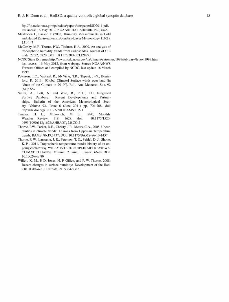
R. J. H. Dunn et al.: HadISD: a quality-controlled global synoptic database 15
ftp://ftp.ncdc.noaa.gov/pub/data/papers/amspaperISD2011.pdf,last access 16 May 2012, NOAA/NCDC, Asheville, NC, USA
Makkonen L, Laakso T (2005) Humidity Measurements in Coldand Humid Environments. Boundary-Layer Meteorology 116(1):131-147
McCarthy, M.P., Thorne, P.W., Titchner, H.A., 2009, An analysis oftropospheric humidity trends from radiosondes, Journal of Cli-mate, 22,22, 5820, DOI: 10.1175/2009JCLI2879.1
NCDC State Extremes http://www.ncdc.noaa.gov/oa/climate/extremes/1999/february/febext1999.html,last access: 16 May 2012, from webpage Source NOAA/NWSForecast Offices and compiled by NCDC, last update 16 March1999
Peterson, T.C., Vautard, R., McVicar, T.R., Thpaut, J.-N., Berris-ford, P., 2011: [Global Climate] Surface winds over land [in”State of the Climate in 2010”]. Bull. Am. Meteorol. Soc. 92(6), p S57.
Smith, A., Lott, N. and Vose, R., 2011, The IntegratedSurface Database: Recent Developments and Partner-ships, Bulletin of the American Meteorological Soci-ety, Volume 92, Issue 6 (June 2011) pp. 704-708, doi:http://dx.doi.org/10.1175/2011BAMS3015.1
Tanaka, H. L., Milkovich, M. L., 1990, MonthlyWeather Review, 118, 1628, doi: 10.1175/1520-0493(1990)118¡1628:AHBAOT¿2.0.CO;2
Thorne, P.W., Parker, D.E., Christy, J.R., Mears, C.A., 2005, Uncer-tainties in climate trends: Lessons from Upper-air Temperaturetrends, BAMS, 86,19,1437, DOI: 10.1175/BAMS-86-10-1437
Thorne, P. W., Lanzante, J. R., Peterson, T. C., Seidel, D. J., Shone,K. P.,. 2011, Tropospheric temperature trends: history of an on-going controversy, WILEY INTERDISCIPLINARY REVIEWS-CLIMATE CHANGE Volume: 2 Issue: 1 Pages: 66-88 DOI:10.1002/wcc.80
Willett, K. M., P. D. Jones, N. P. Gillett, and P. W. Thorne, 2008:Recent changes in surface humidity: Development of the Had-CRUH dataset. J. Climate, 21, 5364-5383.
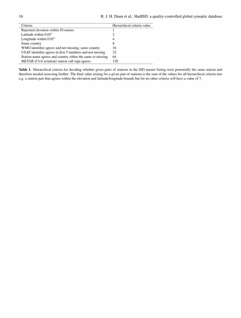
16 R. J. H. Dunn et al.: HadISD: a quality-controlled global synoptic database
Criteria Hierarchical criteria valueReported elevation within 50 metres 1Latitude within 0.05◦ 2Longitude within 0.05◦ 4Same country 8WMO identifier agrees and not missing, same country 16USAF identifier agrees in first 5 numbers and not missing 32Station name agrees and country either the same or missing 64METAR (Civil aviation) station call sign agrees 128
Table 1. Hierarchical criteria for deciding whether given pairs of stations in the ISD master listing were potentially the same station andtherefore needed assessing further. The final value arising for a given pair of stations is the sum of the values for all hierarchical criteria mete.g. a station pair that agrees within the elevation and latitude/longitude bounds but for no other criteria will have a value of 7.
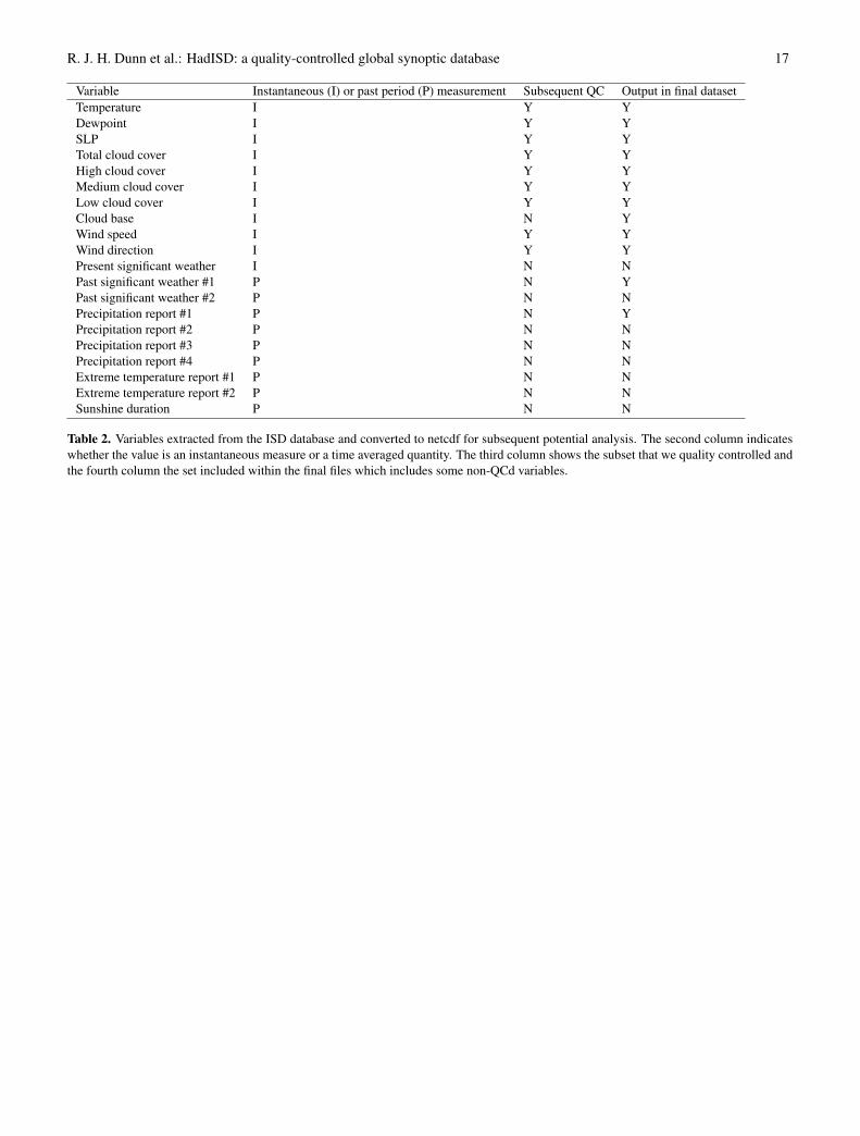
R. J. H. Dunn et al.: HadISD: a quality-controlled global synoptic database 17
Variable Instantaneous (I) or past period (P) measurement Subsequent QC Output in final datasetTemperature I Y YDewpoint I Y YSLP I Y YTotal cloud cover I Y YHigh cloud cover I Y YMedium cloud cover I Y YLow cloud cover I Y YCloud base I N YWind speed I Y YWind direction I Y YPresent significant weather I N NPast significant weather #1 P N YPast significant weather #2 P N NPrecipitation report #1 P N YPrecipitation report #2 P N NPrecipitation report #3 P N NPrecipitation report #4 P N NExtreme temperature report #1 P N NExtreme temperature report #2 P N NSunshine duration P N N
Table 2. Variables extracted from the ISD database and converted to netcdf for subsequent potential analysis. The second column indicateswhether the value is an instantaneous measure or a time averaged quantity. The third column shows the subset that we quality controlled andthe fourth column the set included within the final files which includes some non-QCd variables.

18 R. J. H. Dunn et al.: HadISD: a quality-controlled global synoptic database
Region Temperature Dewpoint Temperature Windspeed Sea-level pressure(◦C) (◦C) (m/s) (hPa)
max min max min max min max minGlobal -89.2 57.8 -100.0 57.8 0.0 113.3 870 1083.3Africa -23.0 57.8 -50.0 57.8 - - - -Asia -67.8 53.9 -100.0 53.9 - - - -S America -32.8 48.9 -60.0 48.9 - - - -N America -63.0 56.7 -100.0 56.7 - - - -Pacific -23.0 50.7 -50.0 50.7 - - - -Europe -58.1 48.0 -100.0 48.0 - - - -Antarctica -89.2 15.0 -100.0 15.0 - - - -
Table 3. Extreme limits for observed variables gained from http://wmo.asu.edu (the official WMO climate extremes repository) andthe GHCND tests. Dewpoint minima are estimates based upon the record temperature minimum for each region. First element ineach cell is the minimum and the second the maximum legal value. Regions follow WMO regional definitions and are given at:http://weather.noaa.gov/tg/site.shtml. Global values are used for any station where the assigned WMO identifier is missing or does notfall within the region categorization. Wind speed and sea-level pressure records are not currently documented regionally so global valuesare used throughout. We note that the value for the African and Global maximum temperature has changed. This will be updated in a futureversion of HadISD.
R. J. H. Dunn et al.: HadISD: a quality-controlled global synoptic database 19
Variable Reporting Resolution Straight repeat streak criteria Hour repeat streak criteria Day repeat streak criteria1◦C 40 values of 14 days 25 days 10 days
Temperature 0.5◦C 30 values or 10 days 20 days 7 days0.1◦C 24 values or 7 days 15 days 5 days1◦C 80 values of 14 days 25 days 10 days
Dewpoint 0.5◦C 60 values or 10 days 20 days 7 days0.1◦C 48 values or 7 days 15 days 5 days1hPa 120 values of 28 days 25 days 10 days
SLP 0.5hPa 100 values or 21 days 20 days 7 days0.1hPa 72 values or 14 days 15 days 5 days1ms1 40 values of 14 days 25 days 10 days
Windspeed 0.5ms1 30 values or 10 days 20 days 7 days0.1ms1 24 values or 7 days 15 days 5 days
Table 4. Streak check criteria and their assigned sensitivity to typical within-station reporting resolution for each variable.

20 R. J. H. Dunn et al.: HadISD: a quality-controlled global synoptic database
Tabl
e5.
Sum
mar
yof
test
sap
plie
dto
the
data
Test
App
lies
toTe
stFa
ilure
Cri
teri
aN
otes
(Num
ber)
TT
dSL
Pw
sw
dcl
ouds
Intr
a-st
atio
nD
uplic
ate
mon
ths
chec
k(2
)X
XX
XX
XC
ompl
ete
mat
chto
leas
tte
mpo
rally
com
plet
em
onth
’sre
cord
forT
Odd
clus
terc
heck
(3)
XX
XX
X≤
6va
lues
in24
hour
sse
para
ted
from
any
othe
rdat
aby>
48ho
urs
Win
ddi
rect
ion
rem
oved
usin
gw
ind
spee
dch
arac
teri
stic
sFr
eque
ntva
lues
chec
k(4
)X
XX
Initi
ally>
50%
ofal
lda
tain
curr
ent
0.5◦
Cor
hPa
bin
out
ofth
isan
d±
3bi
nsfo
ral
ldat
ato
high
light
,with≥
30in
the
bin.
The
non
year
lyba
sis,
usin
ghi
ghlig
hted
bins
with>
50%
ofda
taan
d≥
20ob
serv
atio
nsin
this
and±
3bi
nsO
R>
90%
data
and≥
10ob
serv
atio
nsin
this
and±
3bi
ns.
For
seas
ons,
the
bins
ize
thre
shol
dsar
ere
duce
dto
20,1
5an
d10
resp
ectiv
ely.
His
togr
amap
proa
chfo
rco
mpu
tatio
nal
expe
dien
cy.
Tan
dT
dsy
nerg
istic
ally
rem
oved
,if
Tis
bad,
then
Td
isre
-m
oved
and
vice
vers
a.
Diu
rnal
cycl
ech
eck
(5)
XX
XX
XX
30da
ysw
ithou
t3co
nsec
utiv
ego
odfit
/m
issi
ngor
6da
ysm
ixof
thes
eto
Tdi
urna
lcyc
le.
Dis
trib
utio
nalg
apch
eck
(6)
XX
XM
onth
lym
edia
nan
omal
y>
5IQ
Rfr
omm
edia
n.M
onth
lym
edia
nan
omal
yat
leas
ttw
ice
the
dist
ance
from
the
med
ian
asth
eot
her
tail
and>
1.5
IQR
.D
ata
outs
ide
ofth
eG
auss
ian
dist
ribu
tion
for
each
cale
ndar
mon
thov
eral
lyea
rs,s
ep-
arat
edfr
omth
em
ain
popu
latio
n.
All
mon
ths
inta
ilw
ithap
pare
ntga
pin
the
dist
ribu
tion
are
rem
oved
beyo
ndth
eas
sign
edga
pfo
rth
eva
riab
lein
ques
-tio
n.U
sing
the
dist
ribu
tion
for
allc
al-
enda
rm
onth
s,te
ntat
ive
flags
seti
ffu
r-th
erfr
omm
ean
than
thre
shol
dva
lue.
Toke
epst
orm
s,lo
wSL
Pob
serv
atio
nsar
eon
lyte
ntat
ivel
yK
now
nre
cord
chec
k(7
)X
XX
XSe
eTa
ble
3T
dfla
gged
ifT
flagg
ed.
Rep
eate
dst
reak
s/un
usua
lsp
ell
fre-
quen
cych
eck
(8)
XX
XX
See
Tabl
e4
Clim
atol
ogic
alou
tlier
sch
eck
(9)
XX
Dis
trib
utio
nof
norm
alis
ed(b
yIQ
R)
anom
alie
sin
vest
igat
edfo
rou
tlier
sus
-in
gsa
me
met
hod
asfo
rdi
stri
butio
nal
gap
test
.
Toke
eplo
wva
rian
cest
atio
ns,
min
i-m
umIQ
Ris
1.5C
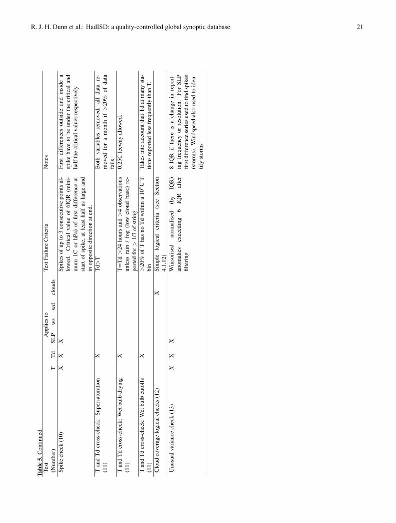
R. J. H. Dunn et al.: HadISD: a quality-controlled global synoptic database 21
Tabl
e5.
Con
tinue
d.Te
stA
pplie
sto
Test
Failu
reC
rite
ria
Not
es(N
umbe
r)T
Td
SLP
ws
wd
clou
dsSp
ike
chec
k(1
0)X
XX
Spik
esof
upto
3co
nsec
utiv
epo
ints
al-
low
ed.
Cri
tical
valu
eof
6IQ
R(m
ini-
mum
1Cor
hPa)
offir
stdi
ffer
ence
atst
arto
fsp
ike,
atle
asth
alf
asla
rge
and
inop
posi
tedi
rect
ion
aten
d.
Firs
tdi
ffer
ence
sou
tsid
ean
din
side
asp
ike
have
tobe
unde
rth
ecr
itica
lan
dha
lfth
ecr
itica
lval
ues
resp
ectiv
ely
Tan
dT
dcr
oss-
chec
k:Su
pers
atur
atio
n(1
1)X
Td>
TB
oth
vari
able
sre
mov
ed,
all
data
re-
mov
edfo
ra
mon
thif>
20%
ofda
tafa
ilsT
and
Td
cros
s-ch
eck:
Wet
bulb
dryi
ng(1
1)X
T=
Td>
24ho
urs
and>
4ob
serv
atio
nsun
less
rain
/fo
g(l
owcl
oud
base
)re
-po
rted
for>
1/3
ofst
ring
0.25
Cle
eway
allo
wed
.
Tan
dT
dcr
oss-
chec
k:W
etbu
lbcu
toff
s(1
1)X
>20
%of
Tha
sno
Td
with
ina
10◦C
Tbi
nTa
kes
into
acco
untt
hatT
dat
man
yst
a-tio
nsre
port
edle
ssfr
eque
ntly
than
T.C
loud
cove
rage
logi
calc
heck
s(1
2)X
Sim
ple
logi
cal
crite
ria
(see
Sect
ion
4.1.
12)
Unu
sual
vari
ance
chec
k(1
3)X
XX
Win
sori
sed
norm
alis
ed(b
yIQ
R)
anom
alie
sex
ceed
ing
6IQ
Raf
ter
filte
ring
8IQ
Rif
ther
eis
ach
ange
inre
port
-in
gfr
eque
ncy
orre
solu
tion.
For
SLP
first
diff
eren
cese
ries
used
tofin
dsp
ikes
(sto
rms)
.W
inds
peed
also
used
toid
en-
tify
stor
ms
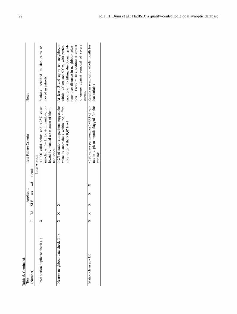
22 R. J. H. Dunn et al.: HadISD: a quality-controlled global synoptic database
Tabl
e5.
Con
tinue
d.Te
stA
pplie
sto
Test
Failu
reC
rite
ria
Not
es(N
umbe
r)T
Td
SLP
ws
wd
clou
dsIn
ter-
stat
ion
Inte
r-st
atio
ndu
plic
ate
chec
k(1
)X
>10
00va
lidpo
ints
and>
25%
exac
tm
atch
overt−
11
tot+
11
win
dow
,fol
-lo
wed
bym
anua
lass
essm
ento
fid
enti-
fied
seri
es
Stat
ions
iden
tified
asdu
plic
ates
re-
mov
edin
entir
ety.
Nea
rest
neig
hbou
rdat
ach
eck
(14)
XX
X>
2/3
ofst
atio
nco
mpa
riso
nssu
gges
tthe
valu
eis
anom
alou
sw
ithin
the
diff
er-
ence
seri
esat
the
5IQ
Rle
vel.
At
leas
t3
and
upto
ten
neig
hbou
rsw
ithin
300k
man
d50
0m,
with
pref
er-
ence
give
nto
fillin
gdi
rect
iona
lqu
ad-
rant
sov
erdi
stan
cein
neig
hbou
rse
lec-
tion.
Pres
sure
has
addi
tiona
lca
veat
toen
sure
agai
nst
rem
oval
ofse
vere
stor
ms.
Stat
ion
clea
nup
(15)
XX
XX
X<
20va
lues
perm
onth
or>
40%
ofva
l-ue
sin
agi
ven
mon
thfla
gged
for
the
vari
able
Res
ults
inre
mov
alof
who
lem
onth
for
that
vari
able
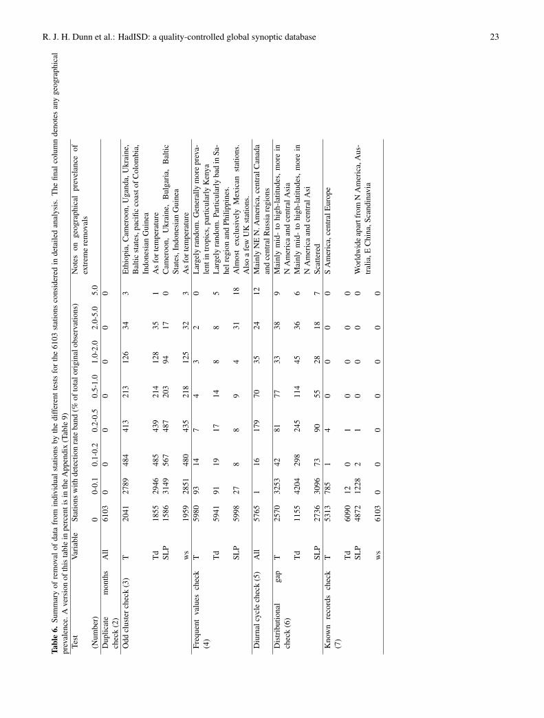
R. J. H. Dunn et al.: HadISD: a quality-controlled global synoptic database 23
Tabl
e6.
Sum
mar
yof
rem
oval
ofda
tafr
omin
divi
dual
stat
ions
byth
edi
ffer
entt
ests
for
the
6103
stat
ions
cons
ider
edin
deta
iled
anal
ysis
.T
hefin
alco
lum
nde
note
san
yge
ogra
phic
alpr
eval
ence
.Ave
rsio
nof
this
tabl
ein
perc
enti
sin
the
App
endi
x(T
able
9)Te
stV
aria
ble
Stat
ions
with
dete
ctio
nra
teba
nd(%
ofto
talo
rigi
nalo
bser
vatio
ns)
Not
eson
geog
raph
ical
prev
elan
ceof
extr
eme
rem
oval
s(N
umbe
r)0
0-0.
10.
1-0.
20.
2-0.
50.
5-1.
01.
0-2.
02.
0-5.
05.
0D
uplic
ate
mon
ths
chec
k(2
)A
ll61
030
00
00
00
Odd
clus
terc
heck
(3)
T20
4127
8948
441
321
312
634
3E
thio
pia,
Cam
eroo
n,U
gand
a,U
krai
ne,
Bal
ticst
ates
,pac
ific
coas
tofC
olom
bia,
Indo
nesi
anG
uine
aT
d18
5529
4648
543
921
412
835
1A
sfo
rtem
pera
ture
SLP
1586
3149
567
487
203
9417
0C
amer
oon,
Ukr
aine
,B
ulga
ria,
Bal
ticSt
ates
,Ind
ones
ian
Gui
nea
ws
1959
2851
480
435
218
125
323
As
fort
empe
ratu
reFr
eque
ntva
lues
chec
k(4
)T
5980
9314
74
32
0L
arge
lyra
ndom
.Gen
eral
lym
ore
prev
a-le
ntin
trop
ics,
part
icul
arly
Ken
yaT
d59
4191
1917
148
85
Lar
gely
rand
om.P
artic
ular
lyba
din
Sa-
helr
egio
nan
dPh
ilipp
ines
.SL
P59
9827
88
94
3118
Alm
ost
excl
usiv
ely
Mex
ican
stat
ions
.A
lso
afe
wU
Kst
atio
ns.
Diu
rnal
cycl
ech
eck
(5)
All
5765
116
179
7035
2412
Mai
nly
NE
N.A
mer
ica,
cent
ralC
anad
aan
dce
ntra
lRus
sia
regi
ons
Dis
trib
utio
nal
gap
chec
k(6
)T
2570
3253
4281
7733
389
Mai
nly
mid
-to
high
-lat
itude
s,m
ore
inN
Am
eric
aan
dce
ntra
lAsi
aT
d11
5542
0429
824
511
445
366
Mai
nly
mid
-to
high
-lat
itude
s,m
ore
inN
Am
eric
aan
dce
ntra
lAsi
SLP
2736
3096
7390
5528
187
Scat
tere
dK
now
nre
cord
sch
eck
(7)
T53
1378
51
40
00
0S
Am
eric
a,ce
ntra
lEur
ope
Td
6090
120
10
00
0SL
P48
7212
282
10
00
0W
orld
wid
eap
artf
rom
NA
mer
ica,
Aus
-tr
alia
,EC
hina
,Sca
ndin
avia
ws
6103
00
00
00
0
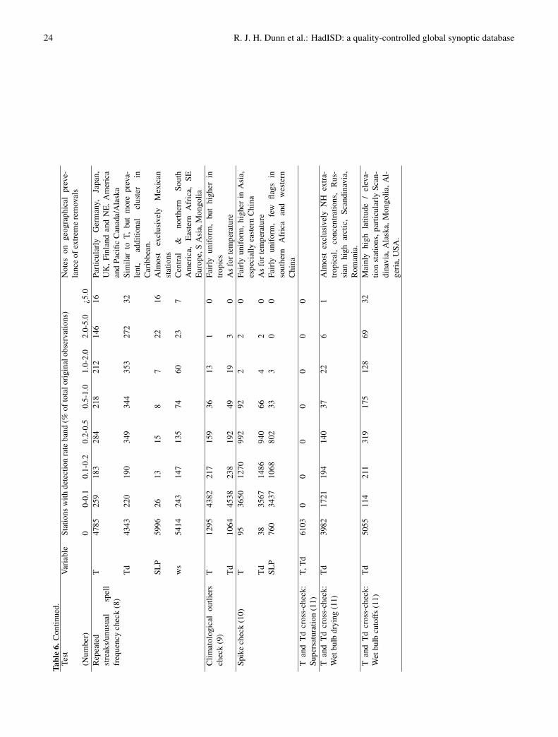
24 R. J. H. Dunn et al.: HadISD: a quality-controlled global synoptic database
Tabl
e6.
Con
tinue
d.Te
stV
aria
ble
Stat
ions
with
dete
ctio
nra
teba
nd(%
ofto
talo
rigi
nalo
bser
vatio
ns)
Not
eson
geog
raph
ical
prev
e-la
nce
ofex
trem
ere
mov
als
(Num
ber)
00-
0.1
0.1-
0.2
0.2-
0.5
0.5-
1.0
1.0-
2.0
2.0-
5.0
¿5.0
Rep
eate
dst
reak
s/un
usua
lsp
ell
freq
uenc
ych
eck
(8)
T47
8525
918
328
421
821
214
616
Part
icul
arly
Ger
man
y,Ja
pan,
UK
,Fi
nlan
dan
dN
E.
Am
eric
aan
dPa
cific
Can
ada/
Ala
ska
Td
4343
220
190
349
344
353
272
32Si
mila
rto
T,bu
tm
ore
prev
a-le
nt,
addi
tiona
lcl
uste
rin
Car
ibbe
an.
SLP
5996
2613
158
722
16A
lmos
tex
clus
ivel
yM
exic
anst
atio
nsw
s54
1424
314
713
574
6023
7C
entr
al&
nort
hern
Sout
hA
mer
ica,
Eas
tern
Afr
ica,
SEE
urop
e,S
Asi
a,M
ongo
liaC
limat
olog
ical
outli
ers
chec
k(9
)T
1295
4382
217
159
3613
10
Fair
lyun
ifor
m,
but
high
erin
trop
ics
Td
1064
4538
238
192
4919
30
As
fort
empe
ratu
reSp
ike
chec
k(1
0)T
9536
5012
7099
292
22
0Fa
irly
unif
orm
,hi
gher
inA
sia,
espe
cial
lyea
ster
nC
hina
Td
3835
6714
8694
066
42
0A
sfo
rtem
pera
ture
SLP
760
3437
1068
802
333
00
Fair
lyun
ifor
m,
few
flags
inso
uthe
rnA
fric
aan
dw
este
rnC
hina
Tan
dT
dcr
oss-
chec
k:Su
pers
atur
atio
n(1
1)T,
Td
6103
00
00
00
0
Tan
dT
dcr
oss-
chec
k:W
etbu
lbdr
ying
(11)
Td
3982
1721
194
140
3722
61
Alm
ost
excl
usiv
ely
NH
extr
a-tr
opic
al,
conc
entr
atio
ns,
Rus
-si
anhi
ghar
ctic
,Sc
andi
navi
a,R
oman
ia.
Tan
dT
dcr
oss-
chec
k:W
etbu
lbcu
toff
s(1
1)T
d50
5511
421
131
917
512
869
32M
ainl
yhi
ghla
titud
e/
elev
a-tio
nst
atio
ns,p
artic
ular
lySc
an-
dina
via,
Ala
ska,
Mon
golia
,Al-
geri
a,U
SA.
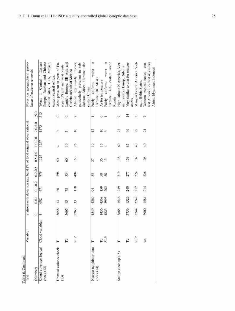
R. J. H. Dunn et al.: HadISD: a quality-controlled global synoptic database 25
Tabl
e6.
Con
tinue
d.Te
stV
aria
ble
Stat
ions
with
dete
ctio
nra
teba
nd(%
ofto
talo
rigi
nalo
bser
vatio
ns)
Not
eson
geog
raph
ical
prev
e-la
nce
ofex
trem
ere
mov
als
(Num
ber)
00-
0.1
0.1-
0.2
0.2-
0.5
0.5-
1.0
1.0-
2.0
2.0-
5.0
¿5.0
Clo
udco
vera
gelo
gica
lch
eck
(12)
Clo
udva
riab
les
168
247
197
911
2413
5711
7331
5W
orst
inC
entr
al/
Eas
tern
Eur
ope,
Rus
sian
and
Chi
nese
coas
tal
site
s,U
SA,
Mex
ico,
east
ern
cent
ralA
fric
a.U
nusu
alva
rian
cech
eck
(13)
T56
5813
8029
850
40
0M
ost
prev
alen
tin
part
sof
Eu-
rope
,US
gulf
and
wes
tcoa
sts
Td
5605
1378
334
6010
30
Lar
gely
Eur
ope,
SEA
sia
and
Car
ibbe
an/G
ulfo
fMex
ico
SLP
5263
3311
849
415
026
109
Alm
ost
excl
usiv
ely
trop
ics,
part
icul
arly
prev
alen
tin
sub-
Saha
ran
Afr
ica,
Ukr
aine
,al
soea
ster
nC
hina
Nea
rest
neig
hbou
rda
tach
eck
(14)
T15
4943
6994
3527
1912
1Fa
irly
unif
orm
,w
orst
inU
krai
ne,U
K,A
lask
aT
d14
5643
6815
958
3616
100
As
fort
empe
ratu
reSL
P18
2339
9520
358
134
61
Fair
lyun
ifor
m,
wor
stin
Ukr
aine
,U
K,
east
ern
arct
icR
ussi
aSt
atio
ncl
ean
up(1
5)T
3865
1546
239
219
138
6027
9H
igh
latit
ude
NA
mer
ica,
Vie
t-na
m,e
aste
rnE
urop
e,Si
beri
aT
d37
5615
2624
027
715
985
4614
Ver
ysi
mila
rto
that
for
tem
per-
atur
esSL
P32
4422
4221
222
410
740
295
Man
yin
Cen
tral
Am
eric
a,V
iet-
nam
,Bal
ticSt
ates
.w
s39
0015
8421
422
610
840
247
Wes
tern
trop
ical
coas
tsce
n-tr
alA
mer
ica,
cent
ral&
east
ern
Afr
ica,
Mya
nmar
,Ind
ones
ia
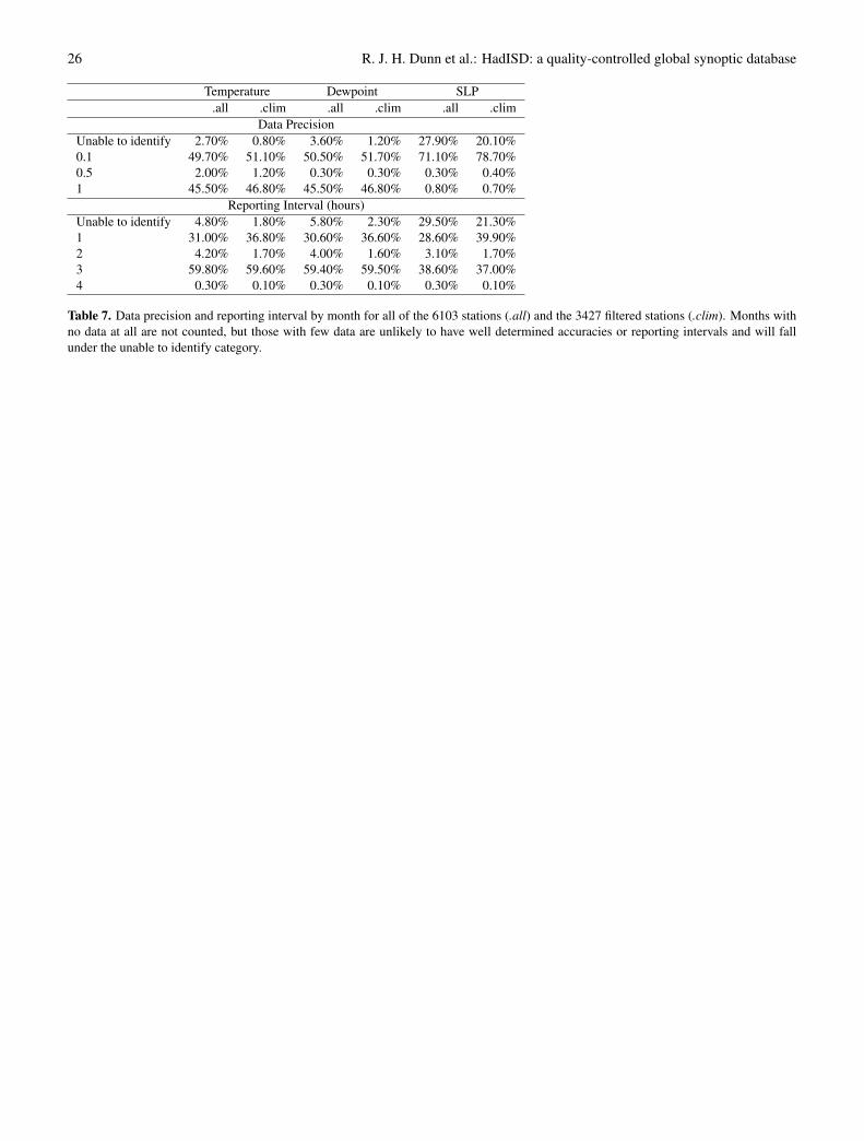
26 R. J. H. Dunn et al.: HadISD: a quality-controlled global synoptic database
Temperature Dewpoint SLP.all .clim .all .clim .all .clim
Data PrecisionUnable to identify 2.70% 0.80% 3.60% 1.20% 27.90% 20.10%0.1 49.70% 51.10% 50.50% 51.70% 71.10% 78.70%0.5 2.00% 1.20% 0.30% 0.30% 0.30% 0.40%1 45.50% 46.80% 45.50% 46.80% 0.80% 0.70%
Reporting Interval (hours)Unable to identify 4.80% 1.80% 5.80% 2.30% 29.50% 21.30%1 31.00% 36.80% 30.60% 36.60% 28.60% 39.90%2 4.20% 1.70% 4.00% 1.60% 3.10% 1.70%3 59.80% 59.60% 59.40% 59.50% 38.60% 37.00%4 0.30% 0.10% 0.30% 0.10% 0.30% 0.10%
Table 7. Data precision and reporting interval by month for all of the 6103 stations (.all) and the 3427 filtered stations (.clim). Months withno data at all are not counted, but those with few data are unlikely to have well determined accuracies or reporting intervals and will fallunder the unable to identify category.

R. J. H. Dunn et al.: HadISD: a quality-controlled global synoptic database 27
Parameter Range considered Final choiceRecord completeness
First data point before 1 Jan 1975–1 Jan 1990 01 Jan 1980Last data point after 31 Dec 1990–31 Dec 2005 31 Dec 2000
Temporal completenessQuartiles of diurnal cycle sampled for day tocount
2–4 3
Days in month for month to count 12,20,28 12Years for a given calendar month present tocount as complete
10,15,20,25,30 20
Number of months passing completeness crite-ria for year to count
9,10,11,12 10
Maximum continuous gap 0,1,2,3,4 years 2 yearsReporting frequency
Median reporting time interval 1,3,6 hours 3 hoursQuality control (all tests applied only if more than 20% of time steps report this variable)
T QC flag prevalence 1,2,5,10% <5%Td QC flag prevalence 1,2,5,10% <5%SLP QC flag prevalence 1,2,5,10% <5%ws QC flag prevalence 10,20,100% <100%wd QC flag prevalence 10,20,100% <100%Cloud total QC flag prevalence 50,100% <100%High cloud QC flag prevalence 50,100% <100%Medium cloud QC flag prevalence 50,100% <100%Low cloud QC flag prevalence 50,100% <100%
Table 8. Station inclusion criteria: ranges considered and final choices. Note that there has been no selection on the wind or cloud variables.These variables have not been the focus of the QC procedure, we therefore do not exclude stations which have valid temperature, dewpointand pressure data on the basis of their wind and cloud data quality.

28 R. J. H. Dunn et al.: HadISD: a quality-controlled global synoptic database
Test Variable Stations within detection rate band (% of total original observations)0 0-0.1 0.1-0.2 0.2-0.5 0.5-1.0 1.0-2.0 2.0-5.0 >5.0
Duplicate months data All 100.0 0.0 0.0 0.0 0.0 0.0 0.0 0.0Isolated cluster T 33.4 45.7 7.9 6.8 3.5 2.1 0.6 0.0
Td 30.4 48.3 7.9 7.2 3.8 2.1 0.6 0.0SLP 26 51.6 9.3 8.0 3.3 1.5 0.3 0.0ws 32.1 46.7 7.9 7.1 3.6 2.0 0.5 0.1
Frequent values T 98.0 1.5 0.2 0.1 0.1 0.0 0.0 0.0Td 97.3 1.5 0.3 0.3 0.2 0.1 0.1 0.1SLP 98.3 0.4 0.1 0.1 0.1 0.1 0.5 0.3
Diurnal cycle All 94.5 0 0.3 2.9 1.1 0.6 0.4 0.2Distributional gap T 42.1 53.3 0.7 1.3 1.3 0.5 0.6 0.1
Td 18.9 68.9 4.9 4.0 1.9 0.7 0.6 0.1SLP 44.8 50.7 1.2 1.5 0.9 0.5 0.3 0.1
Record check T 87.1 12.9 0.0 0.1 0.0 0.0 0.0 0.0Td 99.8 0.2 0.0 0.0 0.0 0.0 0.0 0.0SLP 79.9 20.1 0.0 0.0 0.0 0.0 0.0 0.0ws 100.0 0.0 0.0 0.0 0.0 0.0 0.0 0.0
Repeated streaks / unusual spell frequency T 78.4 4.2 3.0 4.7 3.6 3.5 2.4 0.3Td 71.2 3.6 3.1 5.7 5.6 5.8 4.5 0.5SLP 98.2 0.4 0.2 0.2 0.1 0.1 0.4 0.3ws 88.7 4.0 2.4 2.2 1.2 1.0 0.4 0.1
Climatological outliers T 21.2 71.8 3.6 2.6 0.6 0.2 0.0 0.0Td 17.4 74.4 3.9 3.1 0.8 0.3 0.0 0.0
Spike check T 1.6 59.8 20.8 16.3 1.5 0.0 0.0 0.0Td 0.6 58.4 24.3 15.4 1.1 0.1 0.0 0.0SLP 12.5 56.3 17.5 13.1 0.5 0.0 0.0 0.0
Supersaturation T, Td 100.0 0.0 0.0 0.0 0.0 0.0 0.0 0.0Wet bulb drying Td 65.2 28.2 3.2 2.3 0.6 0.4 0.1 0.0Wet bulb cutoffs Td 82.8 1.9 3.5 5.2 2.9 2.1 1.1 0.5Cloud clean up Cloud variables 0.0 11.2 7.7 16.0 18.4 22.2 19.2 5.2Unusual variance T 92.7 0.2 1.3 4.9 0.8 0.1 0.0 0.0
Td 91.8 0.2 1.9 5.5 1.0 0.2 0.0 0.0SLP 86.2 0.5 1.9 8.1 2.5 0.4 0.2 0.1
Neighbour differences T 25.4 71.6 4.5 0.6 0.4 0.3 0.2 0.0Td 23.9 71.6 2.6 1.0 0.6 0.3 0.2 0.0SLP 29.9 65.5 3.3 1.0 0.2 0.1 0.1 0.0
Station clean up T 63.3 25.3 3.9 3.6 2.3 1.0 0.4 0.1Td 61.5 25 3.9 4.5 2.6 1.4 0.8 0.2SLP 53.2 36.7 3.5 3.7 1.8 0.7 0.5 0.1ws 63.9 26.0 3.5 3.7 1.8 0.7 0.4 0.1
Table 9. As Table 6 but in percentages. Summary of removal of data from individual stations by each test for the 6103 stations in the .alldataset. Each row shows the percentage of stations which had fractional removal rates in the seven bands for the test and variable indicated.
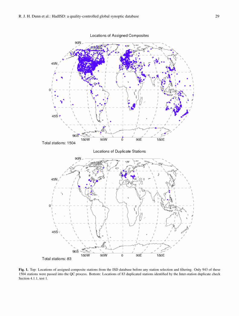
R. J. H. Dunn et al.: HadISD: a quality-controlled global synoptic database 29
Fig. 1. Top: Locations of assigned composite stations from the ISD database before any station selection and filtering. Only 943 of these1504 stations were passed into the QC process. Bottom: Locations of 83 duplicated stations identified by the Inter-station duplicate checkSection 4.1.1, test 1.
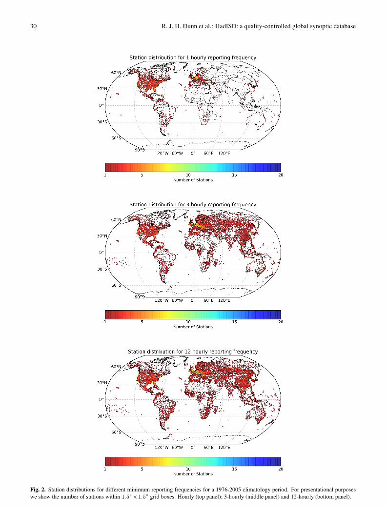
30 R. J. H. Dunn et al.: HadISD: a quality-controlled global synoptic database
Fig. 2. Station distributions for different minimum reporting frequencies for a 1976-2005 climatology period. For presentational purposeswe show the number of stations within 1.5◦×1.5◦ grid boxes. Hourly (top panel); 3-hourly (middle panel) and 12-hourly (bottom panel).
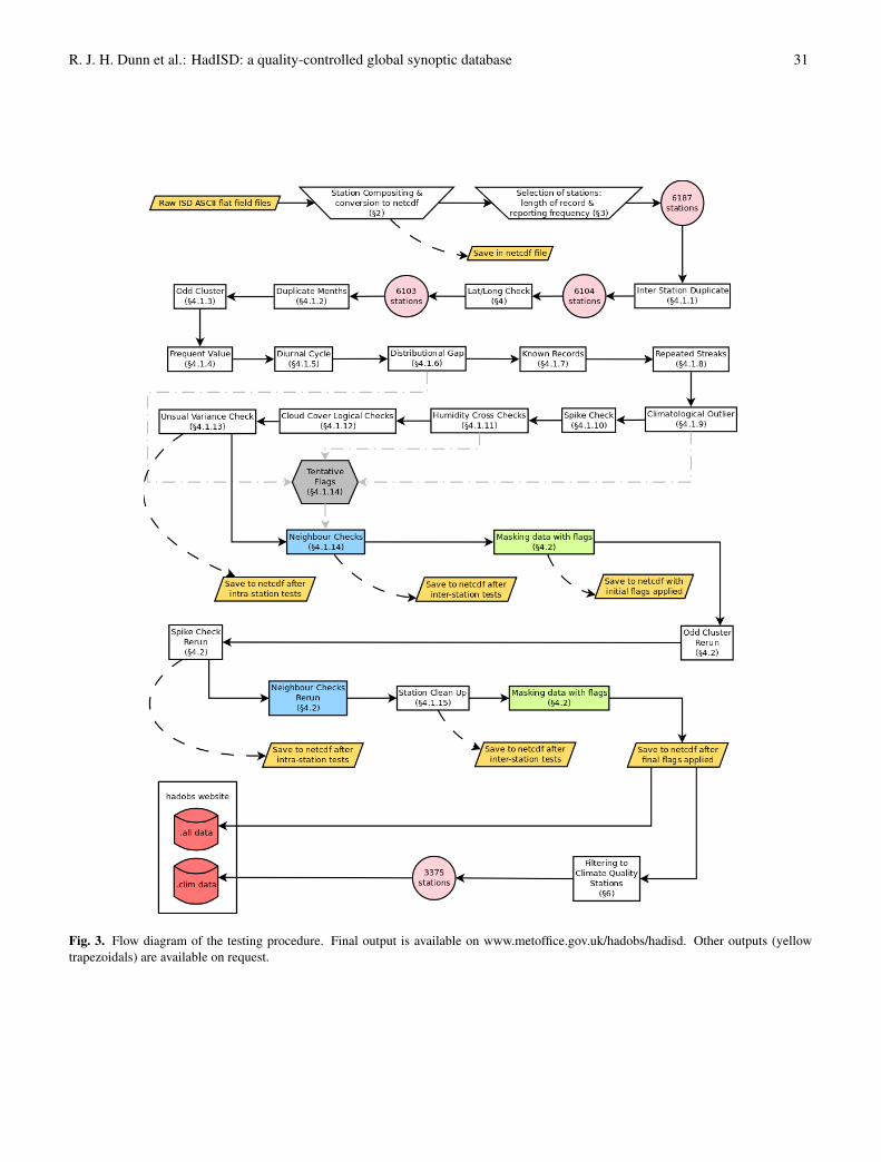
R. J. H. Dunn et al.: HadISD: a quality-controlled global synoptic database 31
Fig. 3. Flow diagram of the testing procedure. Final output is available on www.metoffice.gov.uk/hadobs/hadisd. Other outputs (yellowtrapezoidals) are available on request.
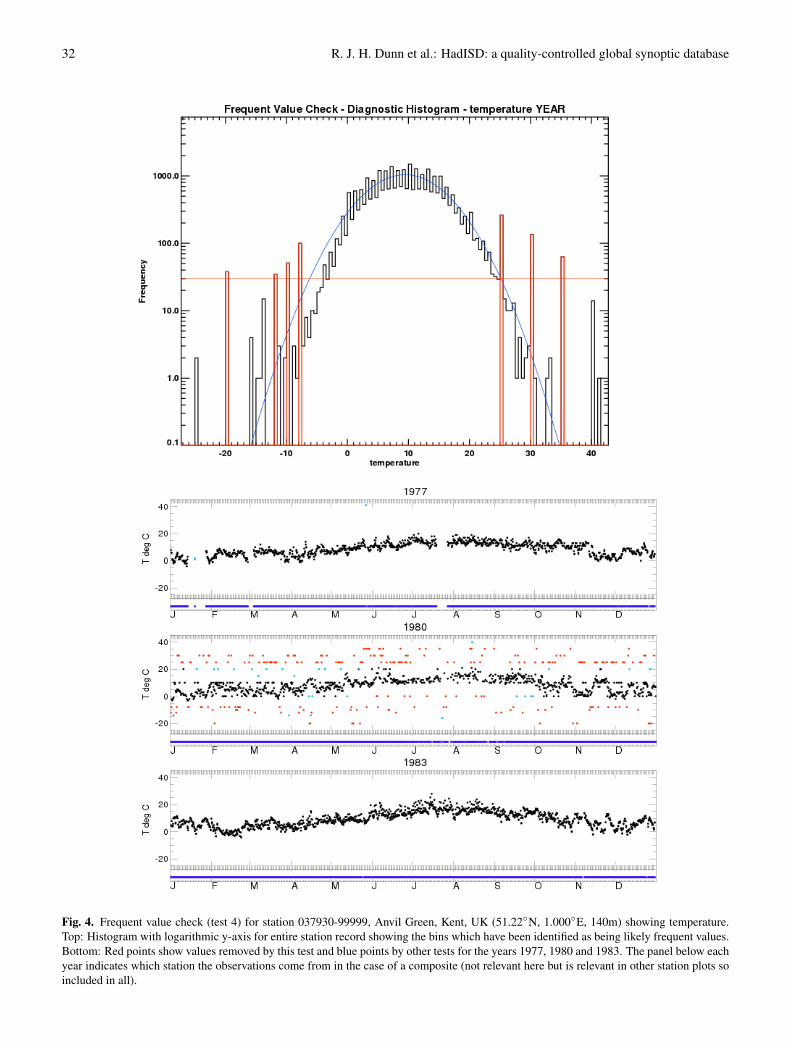
32 R. J. H. Dunn et al.: HadISD: a quality-controlled global synoptic database
Fig. 4. Frequent value check (test 4) for station 037930-99999, Anvil Green, Kent, UK (51.22◦N, 1.000◦E, 140m) showing temperature.Top: Histogram with logarithmic y-axis for entire station record showing the bins which have been identified as being likely frequent values.Bottom: Red points show values removed by this test and blue points by other tests for the years 1977, 1980 and 1983. The panel below eachyear indicates which station the observations come from in the case of a composite (not relevant here but is relevant in other station plots soincluded in all).

R. J. H. Dunn et al.: HadISD: a quality-controlled global synoptic database 33
Fig. 5. Schematic for the diurnal cycle check. (a) An example timeseries for a given day. There are observations in more than 3 quartilesof the day and the diurnal range is more than 5◦C so the test will run. (b) A sine-curve is fitted to the days observations. In this schematiccase, the best fit occurs has a 9 hour shift. The cost function used to calculate the best fit is indicated by the dotted vertical lines. (c) The costfunction distribution for each of the possible 24 offsets of the sine curve for this day. The terciles of the distribution are shown by horizontalblack dotted lines. Where the cost function values enter the second tercile, determines the uncertainty (vertical blue lines). The larger of thetwo differences (in this case 9 to 15=6 hours) is chosen as the uncertainty. So if the climatological value is between 3 and 15 hours, then thisday does not have an anomalous diurnal cycle phase.

34 R. J. H. Dunn et al.: HadISD: a quality-controlled global synoptic database
Fig. 6. Distributional gap check (test 6) example for composite station 714740-99999, Clinton, BC, Canada (51.15◦N, 121.50◦W, 1057m),showing temperature for the years 1974, 1975 and 1984. Red points show values removed by this test and blue points by other tests. Thepanel below each year shows whether the data in the composited station come from the named station (blue) or a matched station (green).There is no change in source station within 1975, and so the compositing has not caused the clear offset observed therein, but the sourcestation has changed for 1984 compared to the other two years.
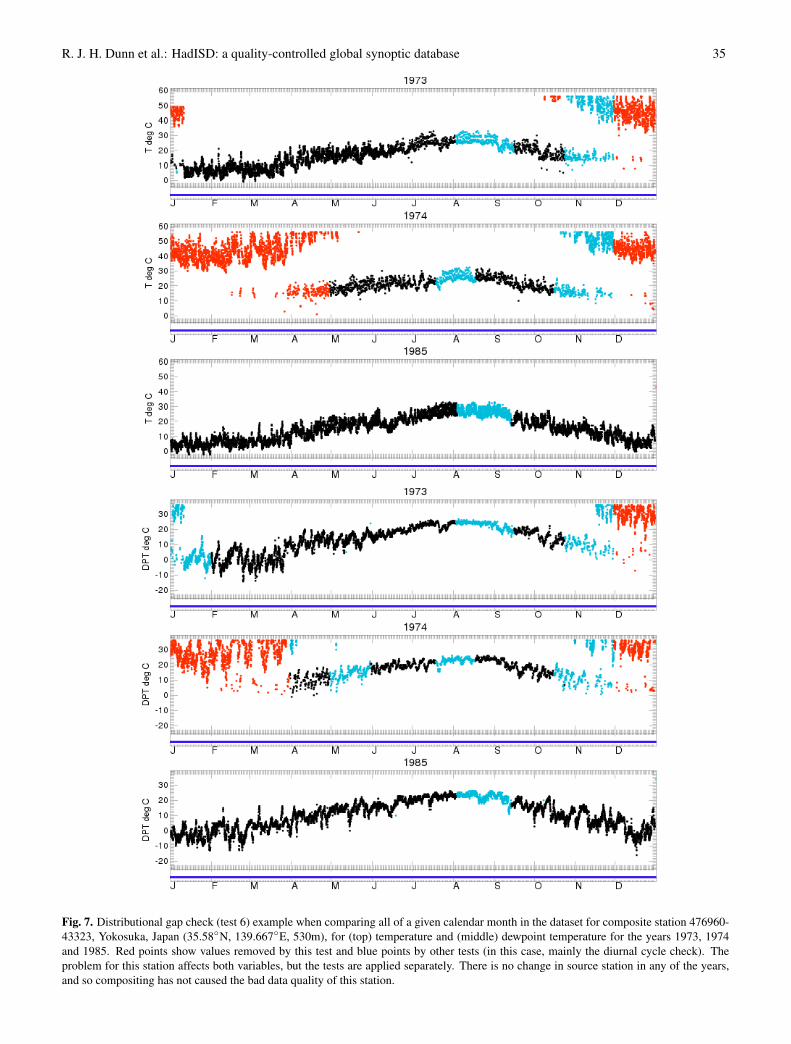
R. J. H. Dunn et al.: HadISD: a quality-controlled global synoptic database 35
Fig. 7. Distributional gap check (test 6) example when comparing all of a given calendar month in the dataset for composite station 476960-43323, Yokosuka, Japan (35.58◦N, 139.667◦E, 530m), for (top) temperature and (middle) dewpoint temperature for the years 1973, 1974and 1985. Red points show values removed by this test and blue points by other tests (in this case, mainly the diurnal cycle check). Theproblem for this station affects both variables, but the tests are applied separately. There is no change in source station in any of the years,and so compositing has not caused the bad data quality of this station.

36 R. J. H. Dunn et al.: HadISD: a quality-controlled global synoptic database
Fig. 8. Distribution of the observations from all Januaries in the station record for composite station 476960-43323, Yokosuka, Japan(35.58◦N, 139.667◦E, 530m). The population highlighted in red is removed by the distributional gap check (test 6), as shown in Fig 7. Notelogarithmic y-axis.
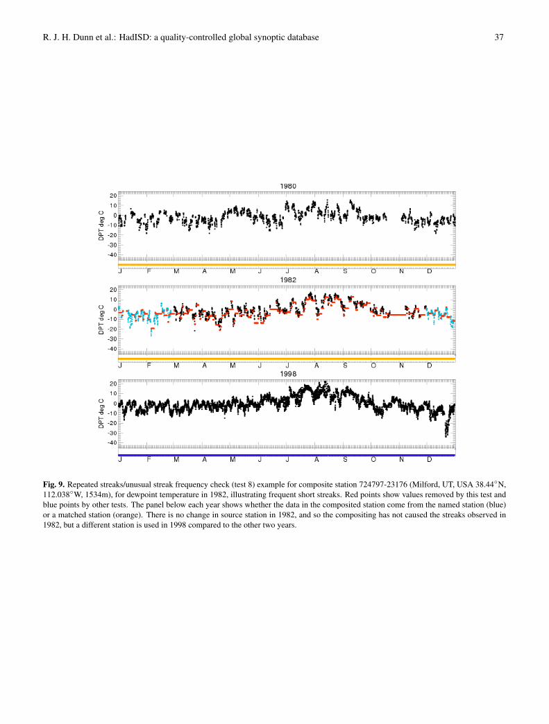
R. J. H. Dunn et al.: HadISD: a quality-controlled global synoptic database 37
Fig. 9. Repeated streaks/unusual streak frequency check (test 8) example for composite station 724797-23176 (Milford, UT, USA 38.44◦N,112.038◦W, 1534m), for dewpoint temperature in 1982, illustrating frequent short streaks. Red points show values removed by this test andblue points by other tests. The panel below each year shows whether the data in the composited station come from the named station (blue)or a matched station (orange). There is no change in source station in 1982, and so the compositing has not caused the streaks observed in1982, but a different station is used in 1998 compared to the other two years.
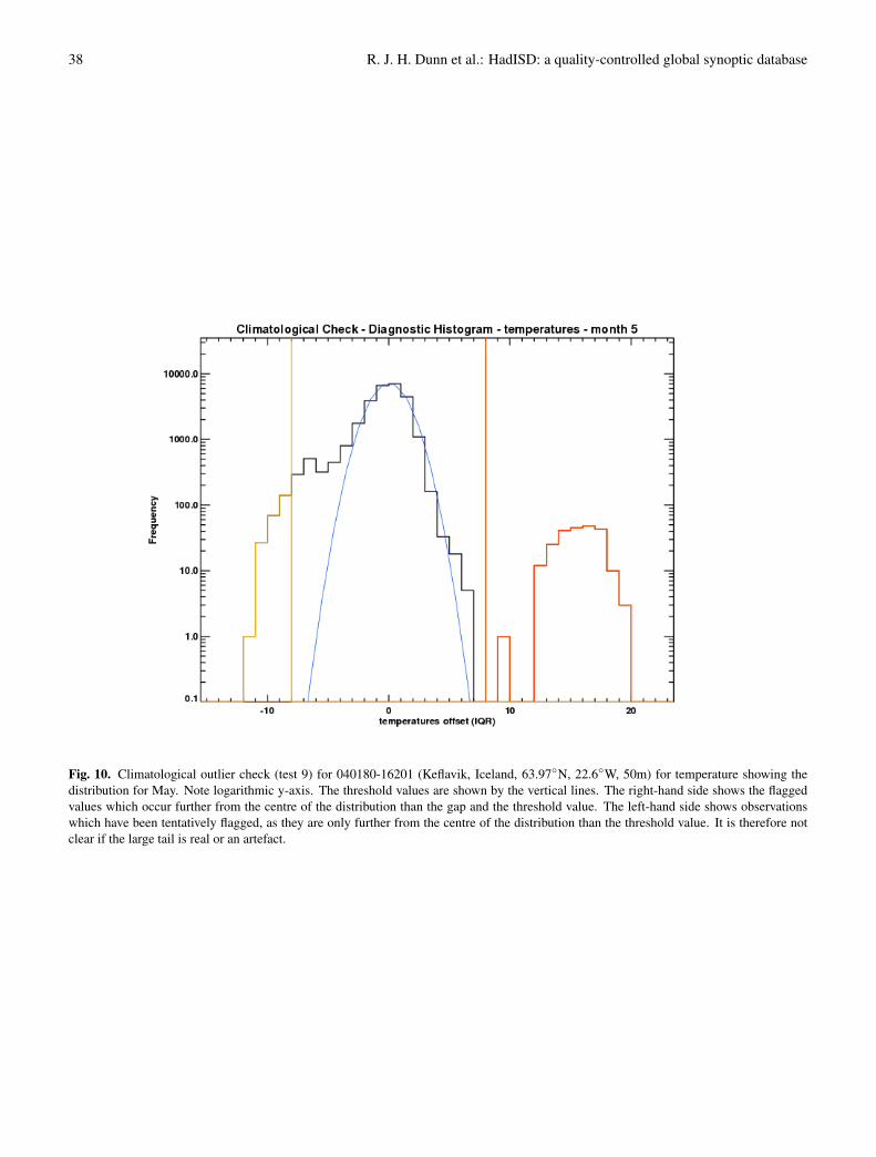
38 R. J. H. Dunn et al.: HadISD: a quality-controlled global synoptic database
Fig. 10. Climatological outlier check (test 9) for 040180-16201 (Keflavik, Iceland, 63.97◦N, 22.6◦W, 50m) for temperature showing thedistribution for May. Note logarithmic y-axis. The threshold values are shown by the vertical lines. The right-hand side shows the flaggedvalues which occur further from the centre of the distribution than the gap and the threshold value. The left-hand side shows observationswhich have been tentatively flagged, as they are only further from the centre of the distribution than the threshold value. It is therefore notclear if the large tail is real or an artefact.
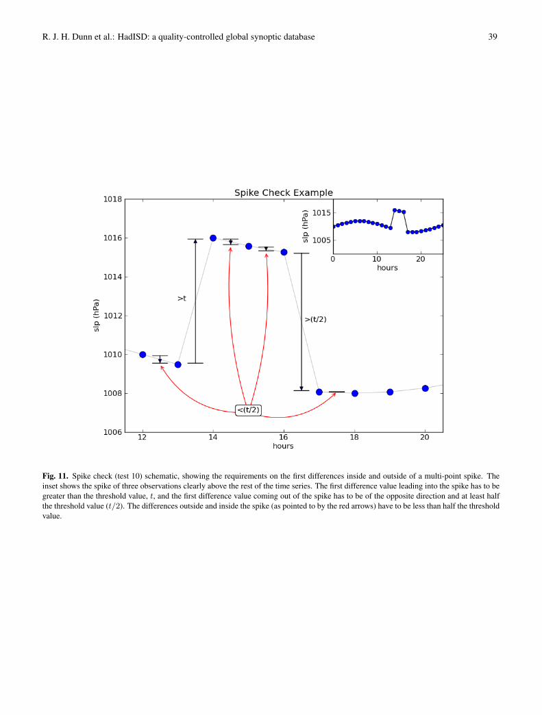
R. J. H. Dunn et al.: HadISD: a quality-controlled global synoptic database 39
Fig. 11. Spike check (test 10) schematic, showing the requirements on the first differences inside and outside of a multi-point spike. Theinset shows the spike of three observations clearly above the rest of the time series. The first difference value leading into the spike has to begreater than the threshold value, t, and the first difference value coming out of the spike has to be of the opposite direction and at least halfthe threshold value (t/2). The differences outside and inside the spike (as pointed to by the red arrows) have to be less than half the thresholdvalue.

40 R. J. H. Dunn et al.: HadISD: a quality-controlled global synoptic database
Fig. 12. Spike check (test 10) for composite station 718936-99999 (49.95◦N, 125.267◦W, 106m, Campbell River, BC, Canada), for dewpointtemperature showing the removal of a ghost station. Red points show values removed by this test and blue points by other tests. The panelbelow each year shows whether the data in the composited station come from the named station (blue) or a matched station (red). In 1988and 2006 a single station is used for the data, but in 1996 there is clearly a blend between two stations (718936-99999 and 712050-99999).In this case the compositing has caused the ghosting, however, but both these stations are labelled in the ISD history file as Campbell River,with identical latitudes and longitudes. An earlier period of merger between these two stations did not lead to any ghosting effects.
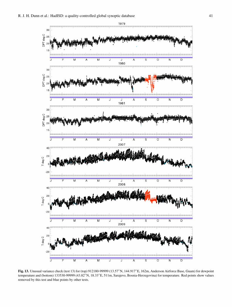
R. J. H. Dunn et al.: HadISD: a quality-controlled global synoptic database 41
Fig. 13. Unusual variance check (test 13) for (top) 912180-99999 (13.57◦N, 144.917◦E, 162m, Anderson Airforce Base, Guam) for dewpointtemperature and (bottom) 133530-99999 (43.82◦N, 18.33◦E, 511m, Sarajevo, Bosnia-Herzegovina) for temperature. Red points show valuesremoved by this test and blue points by other tests.

42 R. J. H. Dunn et al.: HadISD: a quality-controlled global synoptic database
Fig. 14. Nearest neighbour data check (test 14) for 912180-99999 (13.57◦N, 144.917◦E, 162m, Anderson Airforce Base, Guam) for sea-levelpressure. Red points show values removed by this test and blue points by other tests. The spikes for the hurricanes in 1976 and 1977 are keptin the data set. February 1976 is removed by the variance check this February has higher variance than expected when compared to all otherFebruaries for this station.
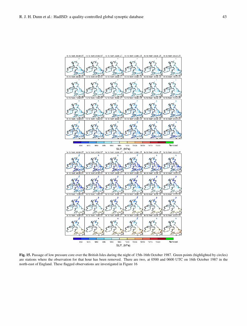
R. J. H. Dunn et al.: HadISD: a quality-controlled global synoptic database 43
Fig. 15. Passage of low pressure core over the British Isles during the night of 15th-16th October 1987. Green points (highlighted by circles)are stations where the observation for that hour has been removed. There are two, at 0500 and 0600 UTC on 16th October 1987 in thenorth-east of England. These flagged observations are investigated in Figure 16
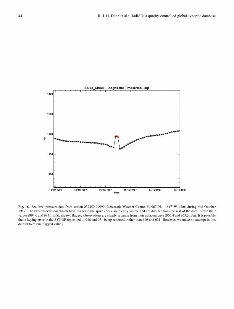
44 R. J. H. Dunn et al.: HadISD: a quality-controlled global synoptic database
Fig. 16. Sea level pressure data from station 032450-99999 (Newcastle Weather Centre, 54.967◦N, -1.617◦W, 47m) during mid-October1987. The two observations which have triggered the spike check are clearly visible and are distinct from the rest of the data. Given theirvalues (994.6 and 993.1 hPa), the two flagged observations are clearly separate from their adjacent ones (966.4 and 963.3 hPa). It is possiblethat a keying error in the SYNOP report led to 946 and 931 being reported, rather than 646 and 631. However, we make no attempt in thisdataset to rescue flagged values.
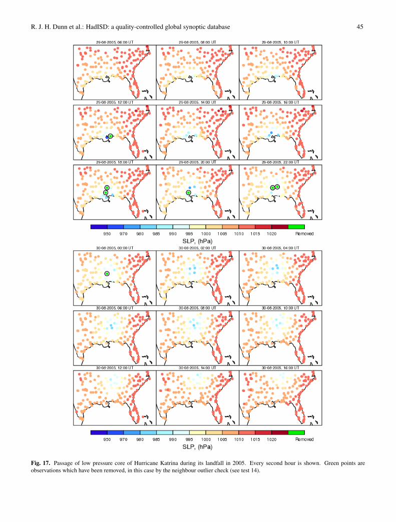
R. J. H. Dunn et al.: HadISD: a quality-controlled global synoptic database 45
Fig. 17. Passage of low pressure core of Hurricane Katrina during its landfall in 2005. Every second hour is shown. Green points areobservations which have been removed, in this case by the neighbour outlier check (see test 14).
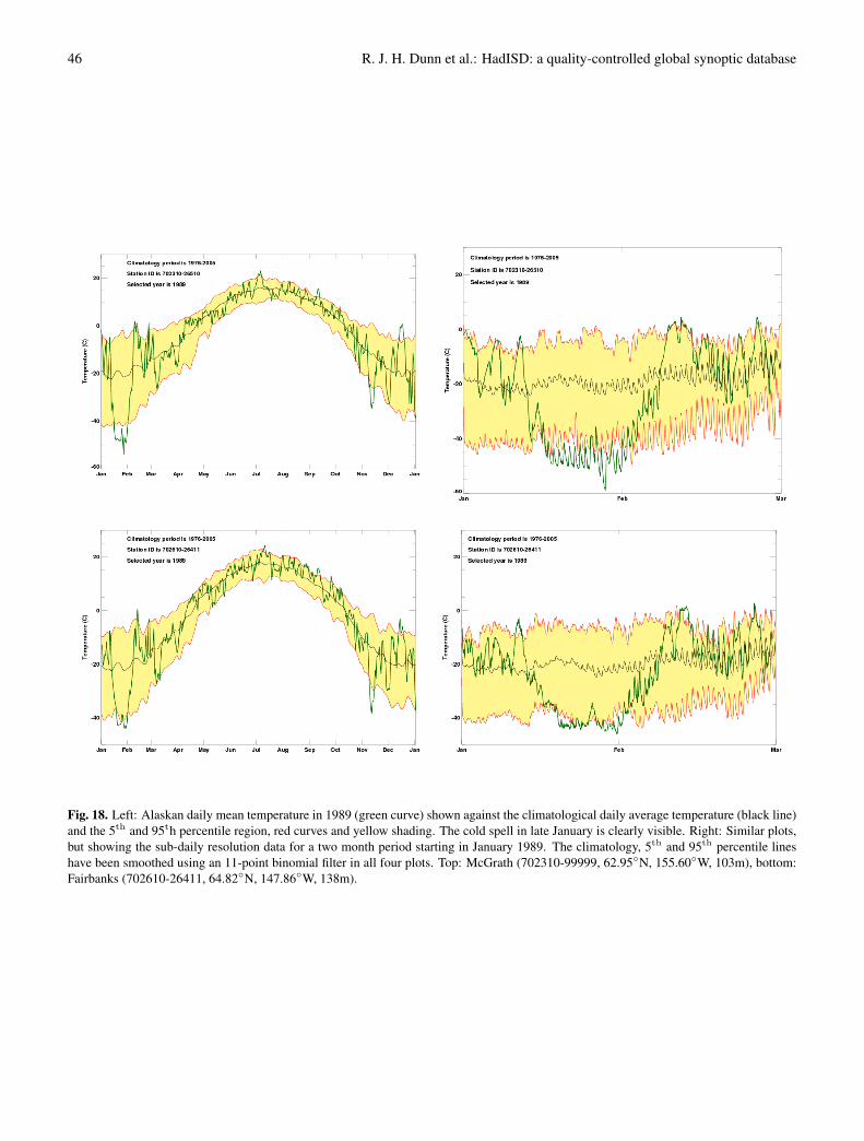
46 R. J. H. Dunn et al.: HadISD: a quality-controlled global synoptic database
Fig. 18. Left: Alaskan daily mean temperature in 1989 (green curve) shown against the climatological daily average temperature (black line)and the 5th and 95th percentile region, red curves and yellow shading. The cold spell in late January is clearly visible. Right: Similar plots,but showing the sub-daily resolution data for a two month period starting in January 1989. The climatology, 5th and 95th percentile lineshave been smoothed using an 11-point binomial filter in all four plots. Top: McGrath (702310-99999, 62.95◦N, 155.60◦W, 103m), bottom:Fairbanks (702610-26411, 64.82◦N, 147.86◦W, 138m).
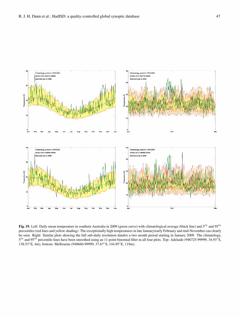
R. J. H. Dunn et al.: HadISD: a quality-controlled global synoptic database 47
Fig. 19. Left: Daily mean temperature in southern Australia in 2009 (green curve) with climatological average (black line) and 5th and 95th
percentiles (red lines and yellow shading). The exceptionally high temperatures in late January/early February and mid-November can clearlybe seen. Right: Similar plots showing the full sub-daily resolution datafor a two month period starting in January 2009. The climatology,5th and 95th percentile lines have been smoothed using an 11-point binomial filter in all four plots. Top: Adelaide (946725-99999, 34.93◦S,138.53◦E, 4m), bottom: Melbourne (948660-99999, 37.67◦S, 144.85◦E, 119m).
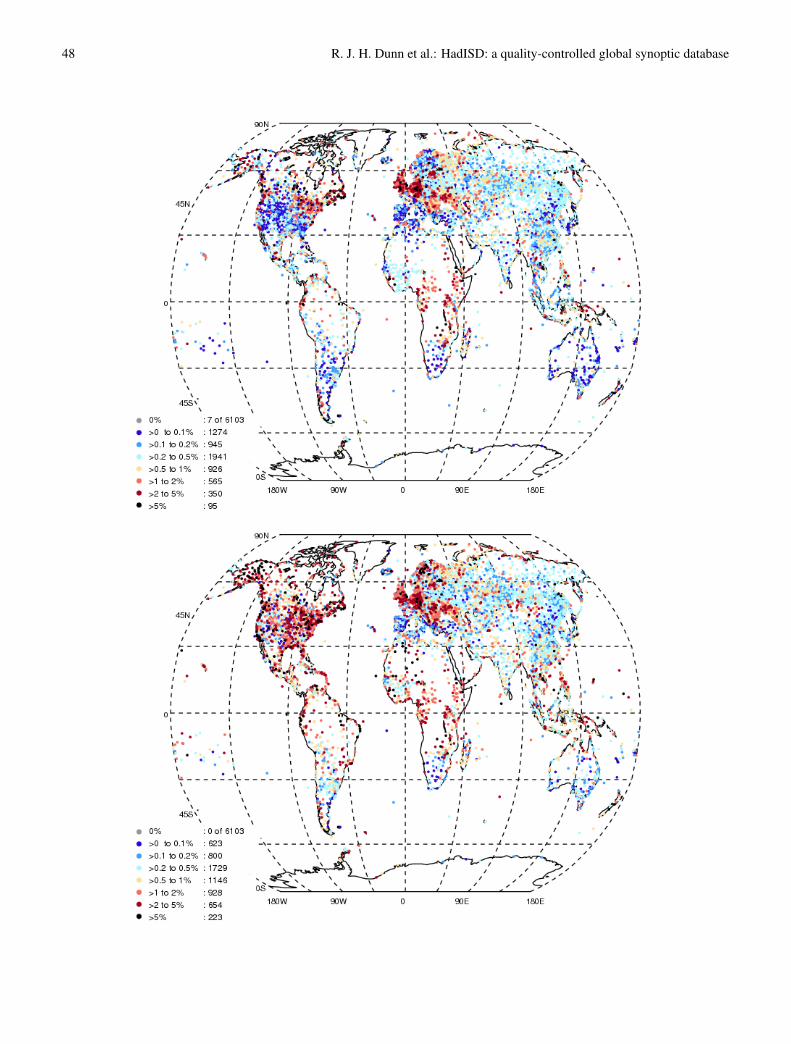
48 R. J. H. Dunn et al.: HadISD: a quality-controlled global synoptic database
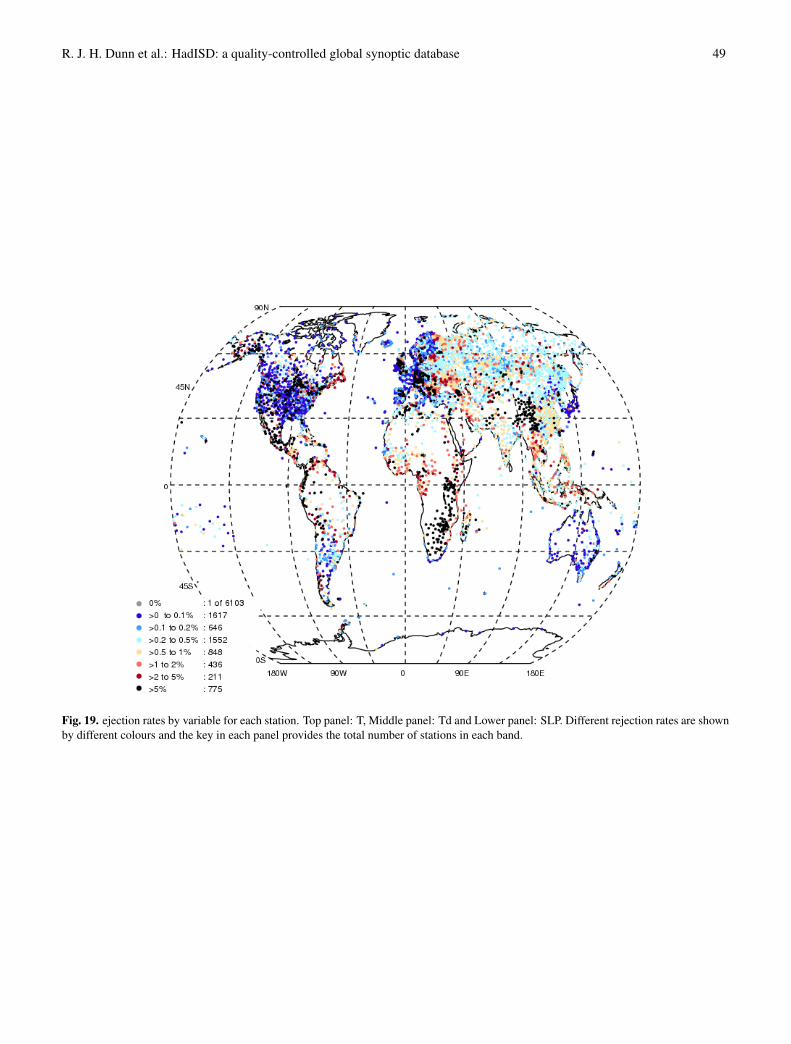
R. J. H. Dunn et al.: HadISD: a quality-controlled global synoptic database 49
Fig. 19. ejection rates by variable for each station. Top panel: T, Middle panel: Td and Lower panel: SLP. Different rejection rates are shownby different colours and the key in each panel provides the total number of stations in each band.
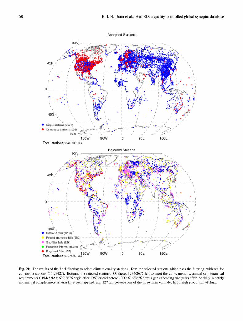
50 R. J. H. Dunn et al.: HadISD: a quality-controlled global synoptic database
Fig. 20. The results of the final filtering to select climate quality stations. Top: the selected stations which pass the filtering, with red forcomposite stations (556/3427). Bottom: the rejected stations. Of these, 1234/2676 fail to meet the daily, monthly, annual or interannualrequirements (D/M/A/IA); 689/2676 begin after 1980 or end before 2000; 626/2676 have a gap exceeding two years after the daily, monthlyand annual completeness criteria have been applied; and 127 fail because one of the three main variables has a high proportion of flags.
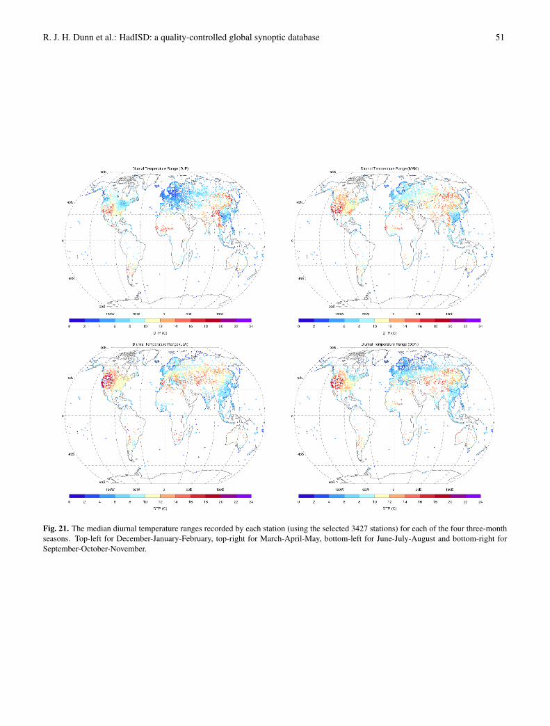
R. J. H. Dunn et al.: HadISD: a quality-controlled global synoptic database 51
Fig. 21. The median diurnal temperature ranges recorded by each station (using the selected 3427 stations) for each of the four three-monthseasons. Top-left for December-January-February, top-right for March-April-May, bottom-left for June-July-August and bottom-right forSeptember-October-November.

52 R. J. H. Dunn et al.: HadISD: a quality-controlled global synoptic database
Fig. 22. The temperature for each station on the 23rd June 2003 at 0000, 0600, 1200 and 1800UT using all 6103 stations.