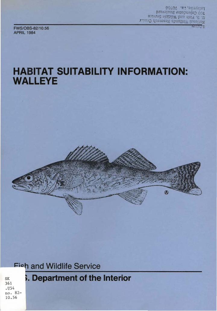
FWS/OBS-82/10.56APRIL 1984

HABITAT SUITABILITY INFORMATION:WALLEYE

__b: i ~

SK361. U54no . 8 2­10.56

and Wildlife Service

. Department of the Interior

HABITAT SUITABILITY INFORMATION: WALLEYE

by

Thomas E. McMahonJames W. Terrell

Habitat Evaluation Procedures Groupand

Patrick C. NelsonInstream Flow and Aquatic Systems Group

Western Energy and Land Use TeamU.S. Fish and Wildlife ServiceDrake Creekside Building One

2627 Redwing RoadFort Collins, CO 80526-2899

Western Energy and Land Use TeamDivision of Biological Services

Research and DevelopmentFish and Wildlife Service

U.S. Department of the InteriorWashington, DC 20240

FWS/OBS-82/10.56Apri 1 1984

This report should be cited as:

McMahon, T. E., J. W. Terrell, and P. C. Nelson. 1984. Habitat suitabilityinformation: Walleye. U.S. Fish Wildl. Servo FWS/OBS-82/10.56. 43 pp.

1981. Standards for the deve 1opment of103 ESM. U.S. Fish Wildl. Serv., Div.

PREFACE

The Habitat Suitability Index (HSI) models presented in this publicationaid in identifying important habitat variables. Facts, ideas, and conceptsobtained from the research literature and expert reviews are synthesized andpresented ~n a format that can be used for impact assessment. The models arehypotheses of species-habitat relationships, and model users should recognizethat the degree of veracity of the HSI model, SI graphs, and assumptions willvary according to geographical area and the extent of the data base forindividual variables. After clear study objectives have been set, the HSImodel building techniques presented in U.S. Fish and Wildlife Service (1981)1and the general guidel ines for modifying HSI model s and estimating modelvariables presented in Terrell et al. (1982)2 may be useful for simplifyingand applying the models to specific impact assessment problems. Simplifiedmodels should be tested with independent data sets, if possible.Statistically-derived models that are an alternative to using SuitabilityIndices to calculate an HSI are referenced in the text.

A brief discussion of the appropriateness of using selected SuitabilityIndex (SI) curves from HSI models as a component of the Instream FlowIncremental Methodology (IFIM) is provided. Additional SI curves, developedspecifically for analysis of walleye habitat with IFIM, also are presented.

Results of a model performance test in a 1imited geographical area aresummarized, but model reliability is likely to vary in different geographicalareas and situations. The U.S. Fish and Wildlife Service encourages modelusers to provide comments, suggestions, and test results that may help usincrease the utility and effectiveness of this habitat-based approach toimpact assessment. Please send comments to:

Habitat Evaluation Procedures Group or Instream Flow andAquatic Systems Group

Western Energy and Land Use TeamU.S. Fish and Wildlife Service2627 Redwing RoadFort Collins, CO 80526-2899

1U.S. Fish and Wildlife Service.habitat suitability index models.Ecol. Servo n.p.

2Terrell, J. W., T. E. McMahon, P. D. Inskip, R. F. Raleigh, and K. L.Williamson. 1982. Habitat suitability index models: Appendix A. Guidelinesfor riverine and lacustrine applications of fish HSI models with the HabitatEvaluation Procedures. U.S. Fish Wildl. Servo FWS/OBS-82/10.A. 54 pp.

iii

iv

CONTENTS

PREFACE iiiFIGURES viACKNOWLEDGMENTS vi i

HABITAT USE INFORMATION................................................ 1Genera 1 1Age, Growth, and Food 1Reproduct ion 1Specific Habitat Requi rements 2

HABITAT SUITABILITY INDEX (HSI) MODELS................................. 5Model Applicability............................................... 5Model Description................................................. 6Model Description - Riverine...................................... 6Model Description - Lacustrine................... 10HSI Calculation................................................... 12Suitability Index (SI) Graphs for Model Variables 12Riverine Model 18Lacustrine Model 24Application of Lacustrine Model................................... 25Interpreting Model Outputs 25

ADDITIONAL HABITAT MODELS 27Modell....................................................... 27Model 2 27Mode 1 3 28Mode 1 4 28

INSTREAM FLOW INCREMENTAL METHODOLOGY (IFIM) 28Suitabil ity Index Graphs as Used in I FIM 28Availability of Graphs for Use in IFIM 30

REFERENCES 37

v

Figure

1

2

3

4

5

6

FIGURES

Tree diagram illustrating relationships between modelvariables, model components, and HSI for the walleyein ri veri ne envi ronments .

Tree diagram illustrating relationships between modelvariables, model components, and HSI for walleye in1acustri ne envi ronments .

SI curves for adult wa 11 eye habitat ..

SI curves for juvenile walleye habitat

Category two SI curves for walleye fry habitat .

SI curves for walleye spawning habitat

vi

7

11

32

33

34

36

ACKNOWLEDGMENTS

We wish to acknowledge the following reviewers who provided many helpfulcomments and suggestions: B. Griswold, Great Lakes National Fisheries ReseachCenter; J. F. Ki tche 11, J. Lyons, and B. John son, Center for Li mno logy,University of Wisconsin, Madison; W. T. Momot, Department of Biology, LakeheadUniversity, Ontario; J. Ney, Virginia Polytechnic Institute and StateUniversity, Blacksburg, Virginia; P. D. Inskip, Harvard University, Boston,Massachusetts; and B. Nelson and D. Rondorf, Seattle National FisheriesResearch Center. W. R. Persons, W. G. Workman, and R. V. Bulkley, Utah StateUniversity, Logan, Utah developed a preliminary draft and bibliography thatprovided useful raw material. C. Short provided editorial assistance. Wordprocessing was by C. J. Gulzow and D. E. Ibarra. K. Twomey assisted infinalizing the manuscript. The cover illustration is from Freshwater Fishesof Canada 1973, Bulletin 184, Fisheries Research Board of Canada, by W. B.Scott and E. J. Crossman.

vii

WALLEYE (Stizostedion vitreum vitreum)

HABITAT USE INFORMATION

Genera 1

The wall eye is native to freshwater ri vers and 1akes of Canada and theUnited States, with rare occurrences in brackish water (Scott and Crossman1973). In the United States, its native range occurs primarily in drainageseast of the Rocky Mountains and west of the Appalachians; however, it has beenwidely introduced into reservoirs outside its native range (Colby et al.1979). Walleye hybridize with sauger (S. canadense) and blue pike (S. v.glaucum) (Scott and Crossman 1973). - - -

Age, Growth, and Food

Walleye live at least 17 years in cool northern waters (Momot pers.comm.); age VIII or younger fish were predominant in Tennessee impoundments(Hackney and Holbrook 1978). Males mature at age II to IV and females at ageIII to VIII (Scott and Crossman 1973; Colby et al. 1979). Growth of walleyedepends primarily on food supply (Swenson and Smith 1976), temperature (Koenstand Smith 1976; Hokanson 1977), and population density (Carlander and Payne1977; Kempinger and Carline 1977). In general, length of sexually maturewalleye (age III+) is> 30 cm (Colby et al. 1979).

Walleye fry eat zooplankton and aquatic insects and start feeding on fishat 1.5 to 2.5 cm in length (Forney 1966; Bul kl ey et al. 1976). The diet ofjuvenile and adult walleye consists primarily of fish, but aquatic inverte­brates, particularly mayfly larvae and crayfish, may be locally or seasonallyimportant (Priegel 1963; Wagner 1972; Johnson and Hale 1977). In northernareas, age 0+ and 1+ yellow perch often account for a large portion of thediet in classic large, shallow perch-walleye lakes (Forney 1977; Kelso andWard 1977). In the southern parts of the walleye range, clupeids andcentrarchids often are most important (Miller 1967; Momot et al. 1977; Fitzand Holbrook 1978). Cannibalism may become significant when other prey arescarce (Chevalier 1973; Forney 1974).

Reproduction

The water temperature regime and the qual ity and quantity of suitablesubstrate are major factors affecting walleye reproductive success (Scott andCrossman 1973; Co 1by et a 1. 1979). Wa 11 eye spawn in spri ng duri ng peri ods of

1

rapid warming soon after ice break-up (Colby et al. 1979). Spawning is usuallyinitiated at water temperatures of 7 to 9° C, with most spawning occurring inthe range of 6 to 11° C (Scott and Crossman 1973). Preferred spawning habitatsare shallow shoreline areas, shoals, riffles, and dam faces with rockysubstrate and good water circulation from wave action or currents (Eschmeyer1950; Johnson 1961; Colby et al. 1979). Lacustrine populations often migrateup rivers to spawn (Priegel 1970).

Walleye spawning activity occurs at night (Ryder 1977) and is often con­centrated within a few days. Eggs are broadcast freely over the substrate andfall into cracks and crevices (Scott and Crossman 1973). Walleye do notprovide any parental care (Balon et al. 1977).

Specific Habitat Requirements

Habitat requirements of walleye have been summarized in reviews in thePERCIS Symposium [J. Fish. Res. Board Can. 34(10) Oct. 1977J and by Kendall(1978), and Colby et al. (1979). Walleye are tolerant of a wide range ofenvironmental conditions (Scott and Crossman 1973) but are generally mostabundant in moderate-to-large lacustrine (> 100 ha) or riverine systemscharacterized by cool temperatures, shallow to moderate depths, extensivelittoral areas, moderate turbidities, extensive areas of clean rocky substrate,and mesotrophic conditions (Kitchell et al. 1977; Leach et al. 1977). Kitchellet al. (1977) suggest that the 1ittoral and subl ittoral habitats occupied bywalleyes in lakes are the equivalent of extensions of suitable riverine habitatinto the lacustrine environment.

Walleye survival, growth, and standing crop have been related to theabundance and availability of the small forage fishes it utilizes as food(Jester 1971; Forney 1974; Swenson and Smith 1976; Momot et al. 1977; Groenand Schroeder 1978). Light conditions also are an important factor affectingwalleye distribution, abundance, and feeding (Ryder 1977). Walleye surviveand grow in a wide range of turbidities (Ali et al. 1977; Ryder 1977), butreach their highest abundance in moderately turbid conditions (Ryder 1968;Elsey and Thomson 1977; Kitchell et al. 1977; Ryder and Kerr 1978). Peakfeeding occurs at water transparencies of approximately 1 to 2 m Secchi diskdepths, with a great decrease in activity at < 1 or > 5 m Secchi disk depths(Ryder 1977). Walleye feed most actively under low light intensity. Lowerstanding crops of walleye in clear lakes may be at least partially attributableto the reduced length of time favorable for feeding (Ryder 1977; Swenson1977). However, this relationship may not always hold in deep, clear lakeswith adequate forage (e.g., cisco or whitefish, Coregonus ~.) available indeep water (Momot pers. comm.).

Walleye fry are photopositive until becoming demersal at lengths of 25 to40 mm (Ney 1978). The demersal fry, juveniles, and adults are very photo­sensitive. They actively seek the shelter of dim light during periods ofstrong light intensities in clear waters (Scherer 1971; Ryder 1977). They areoften found in deep or turbid water or in contact with the substrate undercover of boulders, log piles, brush, and dense beds of submerged vegetationduring the day (Ryder 1977).

2

Walleye are generally most abundant in lakes or lake sections classifiedas mesotrophic (Regier et al. 1969; Kitchell et al. 1977; Leach et al. 1977;Schupp 1978). They are less abundant in oligotrophic conditions (usuallydominated by salmonids) and in eutrophic conditions (usually dominated byce nt r arc hid s ) ( Kit c hell eta1. 1977) . Eut r 0 phi cat ion ten d s t 0 sign if i can t 1yreduce habitat quality for walleye (Kitchell et al. 1977; Leach et al. 1977;Momot et al. 1977; Schupp 1978). Ryder et al. (1974) and Ryder and Kerr(1978), considering only Precambrian Shield lakes of the north temperateboreal forest zone, found walleye to be most abundant in lakes or lake sectionswith morphoedaphic indices (MEl) in the mesotrophic range of about 6.0 to 7.2.Carlander (1977), in contrast, found no correlation between MEl and walleyebiomass in 23 lakes and reservoirs located over a broad geographic range. Heconcluded that the lack of correlation between biomass or yields of walleyeand the usual indicators of productivity (e.g., MEl) was probably due to thefact that walleye populations do not bear a constant relationship to the totalf ish b i omas s 0 r y i e 1d .

Walleye are commonly found in lakes with a pH ranging from 6.0 to 9.0;the species exhibits no behavioral changes when exposed to varying pH levelswithin this range (Scherer 1971). Lower pH levels « 6.0) are associated withfailures in reproduction (Anthony and Jorgenson 1977) and recruitment (Spangleret al. 1977). Higher pH levels (> 9.0) generally are unsuitable for mostfreshwater fish (McKee and Wolf 1963).

Adult. Adult walleye generally are found under cover in moderatelyshall~< 15 m) waters during the day and move inshore at night to feed(Johnson and Hale 1977; Ryder 1977). Adults often are found in areas withslight currents (Ryder 1977), except during the winter when they tend to avoidturbulent areas (Colby et al. 1979). Using the velocity equation developed byJones et al. (1974), the critical velocity (maximum velocity that can besustained for 10 min) for adult walleye 30 em in fork length is 74 em/sec

[critical velocity = (13.07)LO. 51, where L = fork length in cm].

Preferred (optimum) temperatures for grow.th of adults are 20 to 24° C(Dendy 1948; Ferguson 1958; Kelso 1972; Huh et al. 1976). Adults seem toavoid temperatures > 24° C, if possible (Fitz and Ho l br-ock 1978). Kelso(1972) reported that growth in adults ceases at temperatures < 12° C. Upperlethal temperatures of 29 to 32° C were reported by Hokanson (1977), whileWrenn and Forsythe (1978) reported an upper lethal range of 34 to 35° C.Momot et al. (1977) attributed low survival and poor growth of age lV+ fish ina eutrophic central Ohio reservoir to absence of areas of summer habitat withcool « 24° C) water and adequate (> 5 mg/l) dissolved oxygen.

Adult walleye can tolerate dissolved oxygen (DO) levels ofshort time (Scherer 1971), but the greatest abundance of walleyeminimum DO levels are greater than 3 to 5 mg/l (Dendy 1948).< 1 mg/l are 1etha 1 (Scherer 1971).

2 mg/l for aoccurs whereDO 1eve 1s of

Embryo. Highest embryo production and survival has been observed onclean gravel or rubble substrates (2.5 to 15 cm in diameter) (Johnson 1961).Survival also is good on dense mats of vegetation with adequate water circula­tion (Priegel 1970). Percent survival of embryos is greatly reduced on sand,

3

and survival of eggs deposited on soft muck and detritus is negligible (Johnson1961; Priegel 1970). Years of highest embryo production in lakes are oftenassociated with rising or stable spring water levels that increase the amountof littoral area available for spawning and prevent stranding of embryos(Johnson 1961; Chevalier 1977; Groen and Schroeder 1978).

Embryos require well-oxygenated water (Balon et al. 1977), and DO levels~ 5 mg/l are considered necessary for high survival and growth (Oseid andSmith 1971). DO levels s 3.4 mg/l resulted in delayed hatching and a signif­icant reduction in size at hatching (Colby and Smith 1967; Siefert and Spoor1974). Streamflows and wind-generated currents in spawning areas must besufficient for adequate circulation of oxygenated water around embryos (Priegel1970). Positive correlations between spring river discharge and walleye yearclass strength have been reported for several rivers (Nelson and Walburg 1977;Spangler et al. 1977). The nonadhesive eggs can be dislodged from thesubstrate if stream flows or wind-generated currents are too high (Eschmeyer1950; Priegel 1970). In the Great Lakes, the littoral substrate of exposedshoreline areas may be unsuitable for spawning due to strong wave action.Sedimentation (Benson 1968) and anoxia-producing pollutants (Colby and Smith1967) are other factors that can reduce the availability of oxygen and, there­fore, affect the survival of embryos.

Proper maturation of gonads in female walleyes requires minimum winterwater temperatures of < 10° C (Hokanson 1977). Mill er (1967) reported thatwalleyes failed to reproduce in a reservoir with minimum winter temperaturesof 10 to 12.5° C. Embryos are adapted to stead i ly i ncrea sing watertemperatures during the spring. Optimum temperatures are 6 to 9° C forfertilization and 9 to 15° C for incubation (Koenst and Smith 1976). Upperlethal (TL50) temperatures for embryos are near 19° C (Smith and Koenst 1975).

Eggs hatch in 14 to 21 days at temperatures of 8 to 15° C (Ney 1978). Steadyspring warming rates of ~ 0.28° C/day have been positively correlated withembryo and fry production (Busch et al. 1975). Poor survival of embryos isassociated with cold water temperatures due to slow spring warming rates[< 0.18° C/day (Busch et al. 1975)J, cold weather fronts (Busch et al. 1975),or release of cold reservoir water into tailwaters during spawning and incuba­tion (Pfitzer 1967).

Fry. Stream velocities in spawning tributaries must be sufficient totransport fry downstream to lakes within the period of yolk-sac absorption (3to 5 days) or fry will perish from lack of food (Priegel 1970). Fry will notbegin to feed at temperatures < 15° C (Smith and Koenst 1975). Momot et al.(1977) reported that stocked walleye fry exhibited greater survival when therewas a high availability of newly hatched gizzard shad (Dorosoma cepedianum) attime of stocking.

Optimum temperatures for growth of walleye fry are near 22° C (Kelso1972; Huh et al. 1976; Koenst and Smith 1976). No growth occurs at tempera­tures s 12° C or ~ 29° C (Kelso 1972; Hokanson 1977). Upper lethal tem­peratures for fry are in the range of 31 to 33° C (Smith and Koenst 1976;Wrenn and Forsythe 1978). Conditions that reduce or retard growth (e.g., low

4

temperature, low zooplankton abundance, and delayed hatching) can greatlyaffect fry overwinter survival because smaller fry experience more overwintermortality than larger fry (Forney 1966).

Optimum DO concentrations for fry are ~ 5 mg/l (Siefert and Spoor 1974).Moyle and Clothier (1959) reported that DO levels below 5 mg/l resulted inpoor survival of stocked fry. Low DO levels also retard fry development(Oseid and Smith 1971) and reduce swimming ability (Siefert and Spoor 1974).

Fry can withstand only slight current velocities (Houde 1969). Walburg(1971) and Groen and Schroeder (1978) reported that high velocities near areservoir outlet can result in significant fry losses, particularly if spawningoccurs at the dam face.

Juvenile. Habitat requirements for juvenile walleye seem to be similarto those of adults (Colby et al. 1979). Using the previously described regres­sion equation from Jones et al. (1974), the critical velocity for juvenileswi th a fork 1ength of 20 cm is 60 cm/ sec.

HABITAT SUITABILITY INDEX (HSI) MODELS

Model Applicability

Geographic area. This model is applicable to North American waterswithin the native and introduced range of walleye. The standard of comparisonfor each variable is the optimum value of the variable that occurs anywherewithin this area. Optimum conditions will most likely occur in the northernUnited States, southern Canada, or within the median temperature envelopeboundaries of percids, as defined by Hokanson (1977).

Season. The model provides an index for a riverine or lacustrine habitatbased on its ability to support all life stages of walleye throughout theyear.

Cover types. The model is app 1 i cab1e in ri veri ne, 1acustri ne, andpalustrine habitats, as described by Cowardin et al. (1979).

Minimum habitat area. Minimum habitat area is defined as the mt nnnumarea of contiguous, suitable habitat that is required to sustain a population.The minimum habitat area required by walleye populations is unknown, butrelatively large lakes (> 100 ha) or river systems are more likely to provideadequate conditions for spawning (Kitchell et al. 1977; Leach et al. 1977).Self-sustaining walleye populations are generally rare in small lakes that arenot connected to other lakes (Johnson et al. 1977). However, walleye areoften abundant in small lakes « 400 ha), where natural reproduction issupplemented by stocking (J. Lyons, pers. comm.; B. Johnson, pers. comm).Kitchell et al. (1977) noted that while walleye were present in many small« 100 ha) lakes, they were abundant in only a few.

5

Verifi cat ion 1eve 1. The model represents our i nterpretat i on of howselected environmental factors limit potential carrying capacity. Portions ofthe model have been subjected to limited field application, by comparison withstanding crop and catch per unit effort data. Reviewers of the model haverecommended extensive testing and evaluation before accepting the model, orport ions of the mode 1, based on suitabi 1ity index graphs as an accuratepredictor of habitat quality. We agree with these recommendations.

Model Description

The Habitat Suitability Index (HSI) model that follows has two versions:riverine and lacustrine. These two versions condense the preceding observa­tions into a set of measurable habitat variables. The model is structured toproduce an index of walleye habitat quality between 0.0 (unsuitable) and 1.0(optimum). A positive relationship between HSI and carrying capacity isassumed but has not been demonstrated. Habitat variables believed to beimportant in limiting distribution, abundance, or survival of walleye areincluded in the models. An assumed functional relationship between eachhabitat variable and habitat suitability is represented in a variable suitabil­ity index (SI) graph. It is assumed that SI ratings for different habitatvariables can be compared. This is one of the weakest model assumptions. Itis likely to be violated for some ranges of the selected variables because theimpacts (e.g., changes in growth rates, survival rates, distribution, andabundance) measured by each variable are not directly comparable. The modelis likely to provide the most accurate description of carrying capacity whenall of the variables have extreme SI values; i.e., either near optimum orunsuitable.

Walleye habitat quality is represented by food, cover, water quality, andreproductive components. Variables that are thought to be direct or indirectmeasures of the relative ability of a habitat to meet these requirements areincluded in the appropriate component. Variables that affect habitat qualityfor walleyes, but do not easily fit into one of these four major components,are combined under the "other component." heading.

It should be noted that not all variables that potentially affect walleyepopulations are included in the models. Variables were not included if:(1) the variable was adequately measured by another variable(s); or (2) itwould be difficult to measure the variable quantitatively [e.g., effects ofinter- and intraspecific interactions on walleye biomass (Forney 1977)J.

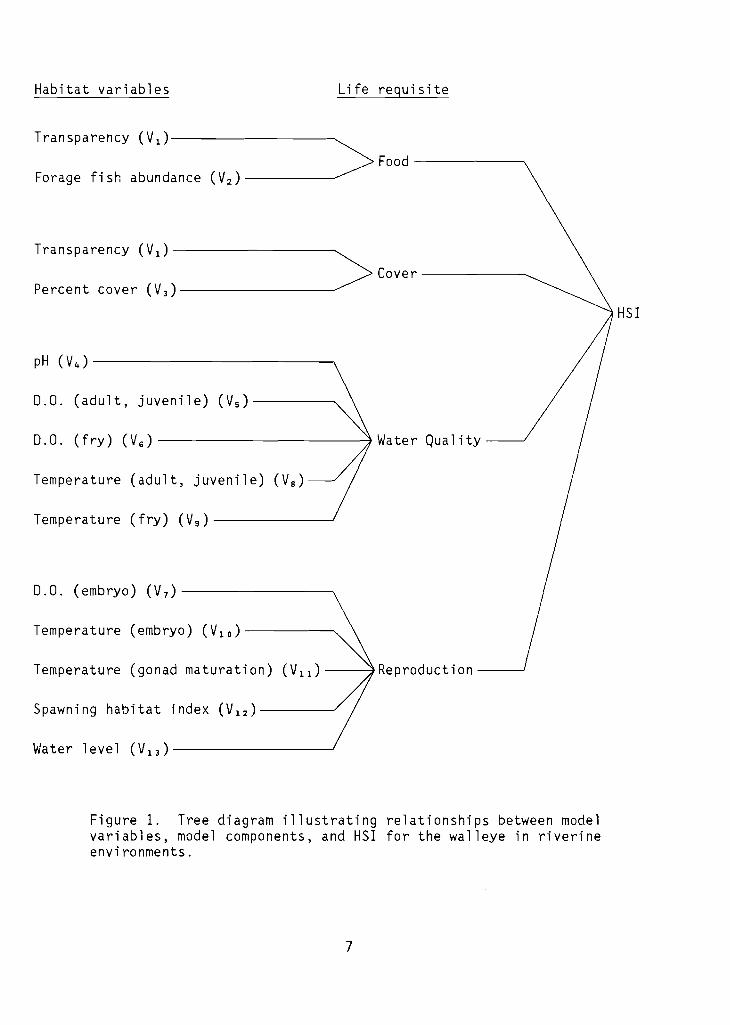
Model Description - Riverine

The structure of the riverine HSI model for walleye is presented graph­ically in Figure 1.

Food component. Average Secchi disk depth (V1 ) is considered part of the

food component because feeding activity is related to transparency (light)conditions. The optimum transparency range depicted in the graph is reasonablywell defined in the literature from observations of conditions associated with

6

Habitat variables Life requisite

Transparency (Vl)----------------~>Food ----------,Forage fish abundance (V2)--------~

Transparency (V 1 ) ------------------->Cove r ------------.....Percent cover (V3)----------------~·

HSI

pH (V 4) -------------.

D.O. (fry) (V 6 ) ---------------iWater Quality---'

Temperature (gonad maturation) (V ll ) --~Reproduction ------'

D.O. (embryo) (V 7 ) -------~

Temperature (fry) (V 9 ) ---l

D.O. (adult, juvenile) (V s ) ---------..

Temperature (adult, juvenile) (Va)

Temperature (embryo) (V10)--------~

Spawning habitat index (V 1 2 ) - - - -J

Water level (V13)----------------~

Figure 1. Tree diagram illustrating relationships between modelvariables, model components, and HSI for the walleye in riverineenvironments.

7

high feeding levels. Walleyes occur in very clear waters, although the timeavailable for efficient foraging is reduced in those lakes that lack deepwater and deep-water prey, such as cisco (Ryder 1977; Momot, pers. comm.). Itwas assumed that walleyes can find some shelter from light even in very clearwaters, either in the form of cover or deep water; therefore, the descendinglimb of the graph remains above zero. Too much turbidity favors competitors,such as centrarchids (Kitchell et al. 1977), and apparently results in reducedfeeding efficiency (Ryder 1977). Although some feeding probably occurs athigh turbidity levels, the graph descends to 0 at very low Secchi disk depths,because it was assumed that clogging and abrasion of gills or high embryomortality would occur at these levels.

The relative abundance of forage fishes (V2 ) was included in this

component because growth, food consumption, and standi ng crop of wa 11 eye arerelated to forage abundance. The index of relative abundance was measured inunits of mg/m 3 of prey density, after Swenson and Smith (1976).

Variables V1 and V2 are assumed to be direct measures of food avail­

ability. Therefore, an increase in the suitability of either food componentvariable is assumed to increase the amount of available food by the sameamount, regardless of the other food component variable rating. This assump­tion is expressed by combining variables through a simple arithmetic mean.

Cover component. The cover component was broken down into two subcompo­nent ratings, based on the amount of cover related to light conditions andcover in the form of physical shelter. Transparency (V1 ) is included in a

light intensity subcomponent because standing crop of walleye is reduced in:(1) clear water without sufficient water depth to provide cover from brightlight; or (2) in very turbid waters where sauger (S. canadense) or centrarchidspredominate (Leach et al. 1977; Ryder 1977). Percent of area with cover (V3 )

is included in both subcomponents because cover is used both as an escape fromintense light levels and as a resting area to avoid high water velocities.

The importance of percent cover (V 3 ) for shelter from light is assumed to

vary. When transparency is too high to be optimum (Secchi disk transparency> 3.2 m), cover should become more important in determining habitat qualitybecause the clearer the water, the greater the need to have cover to escapefrom high light intensities. These assumptions are quantified by combiningthe two variable ratings into a subcomponent of cover related to the abilityof a water body to provide shelter from light. The coefficients in the equa­tion quantify these subjective opinions; they are not the result of rigorousexperimentation.

If the Secchi transparency is < 3.4 m (3.4 m rates an SI of 0.9), thesubcomponent equals:

8

This equation reflects the greater importance of transparency (VI) in deter­

mining habitat quality in terms of cover from light in waters that have nearoptimum or lower than optimum transparency levels. It could be ctrgued that,when water transparency is too low to be optimum, percent cover should not beincluded in a subcomponent rating depicting cover from light. Percent coverwas left in the equation because transparency levels can be variable and COV2rcan occasionally become important in water that normally has transparencylevels too low to be optimum. If the Secchi transparency is greater than3.4 m, the SI rating is less than 0.9 and is determined from the descendinglimb of the SI curve for VI' In this situation, the subcomponent equals:

where N = [10(1-S1 of VI)]' The second equation provides the same answer as

the first equation when VI has an SI of 0.9. It predicts a slower drop in

suitability when increasing transparency is associated with high cover ratingsthan when it is associated with low cover ratings. The equation thusquantifies the assumption that cover is more important for shelter from lightwhen the water is too clear to be optimum.

Water quality component. Dissolved oxygen (Vs, V6 ) and temperature (Va,

V9 ) levels for adults-juveniles and fry, respectively, as well as pH (V 4 ) , are

i ncl uded because these water qua1i ty parameters affect growth, survi va1, orfeeding (or all three) in walleye. Suboptimum levels of these variables aredefined primarily from well-documented negative impacts that do not appear tobe mitigated by a higher suitability of other variables. This, and the factthat the dependency of dissolved oxygen requirements on temperature is includedin the variable definition, justifies combining these variables into a sub­component rating by selecting the lowest variable rating.

Reproduction component. Dissolved oxygen (V 7 ) , mean weekly temperatures

in spring (V lO ), and minimum winter water temperatures (V ll ) are included in

this component because they can be limiting factors to successful embryosurvival or gamete development. Quantity (percent riffles in riverine situa­tions or littoral area in lacustrine situations) and quality (substrate type)of spawning habitat have been shown to affect embryo survival and productionand, therefore, are included in a spawning habitat index (V I 2 ) based on the

product of quantity (percent riffle or littoral area> .3 m but < 1.5 m deep)and qual ity (determined from a substrate index) of spawning habitat. Modelusers may want to modify the depth criteria based on available data for localwalleye populations.

9

In order to interpret the spawn i ng habi tat index, it is necessary toassume some optimum quantity of spawning habitat needed to ensure maximumreproductive success. This quantity is likely to vary for different types ofwater bodies in different geographic areas, and the impact of a change inspawning area is likely to be difficult to evaluate. For example, Buschet al. (1975) found that, while suitable spawning habitat (and walleye popula­tions) in western Lake Erie had been substantially reduced from historicallevels, the remaining spawning reef area of 51.3 to 110.4 ha (depending onwater level) was still capable of producing strong year classes of walleye inthe western basin. However, the limited spawning habitat appeared to be afactor in making spawning success more vulnerable to variations in weather. Ahigh value (20%) was selected as the optimum proportion of a water body thatshould meet the criteria for spawning. Model users should critically evaluatethe suggested percentage and modify it based on local data. Multiplication ofthe derived spawning substrate index (e.g., 0.20) by the maximum possiblespawning substrate index (e.g., 200, derived by multiplying 100% rubble timesthe proposed weighting factor of 2) obtainable for a specified area resultedin a product of 40 (see spawning habitat index V1 2 ) . Therefore, 40 was defined

as the optimum value of the spawning habitat index (V 12 ) and a suitability

index of 1.0 was assigned to all spawning habitat indices ~ 40. A spawninghabitat index of 0 was equated to an H5I of 0 because 0 was believed to repre­sent conditions where the likelihood of successful reproduction is nil (e.g,100% silt = spawning habitat index of 0).

Water level during the spawning period (V 13 ) is also included in this

component because the water level can affect the area and type of substrateavailable for spawning; it has also been related to year-class strength. Asuboptimum water level fluctuation was assumed to consistently have a negativeimpact on reproductive success; this is especially so because walleye spawningis restricted to a relatively short time period in the spring.

Compensation among reproduction variables was considered unlikely; there­fore, the lowest variable rating among the combined variables was selected asthe subcomponent value.

H5I calculation. The H5I was defined as the minimum value for anycomponent 51 because "s ubop t imurn" conditions for a component were assumed torepresent conditions that have measurable negative impacts on individuals andthus limit carrying capacity even when other conditions are optimum.

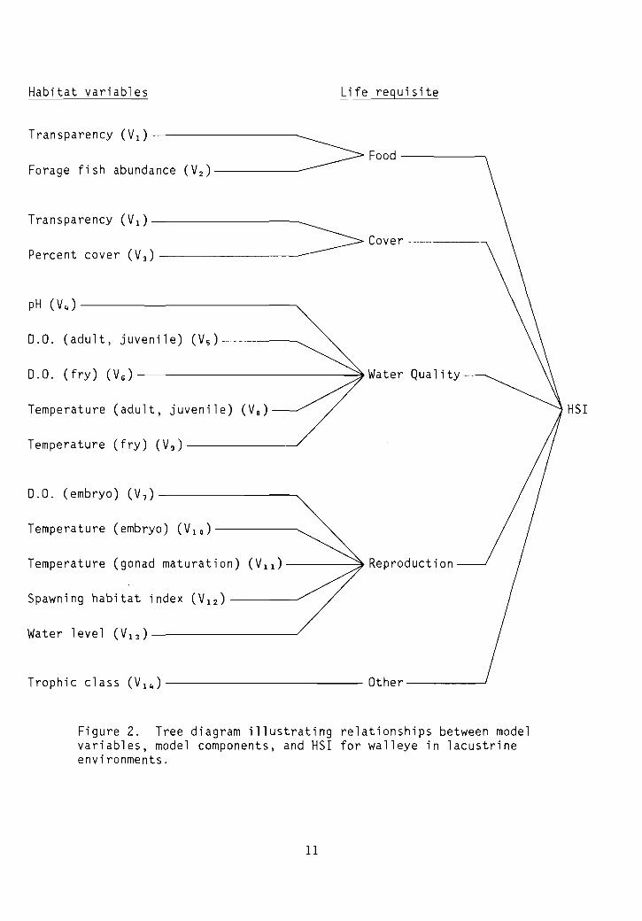
Model Description - Lacustrine

The structure of the lacustrine H5I model for walleye is shown inFigure 2. The model includes the components from the riverine model, withan "o the r" component added to the mode1.

\lOther\l component. A measure of the trophic status of a lake (V 1 4 ) is

assumed to be a general determinant of habitat suitability for walleye becauseabundance of walleye often has been related to trophic conditions. Trophicstatus is a composite variable that includes many of the factors that appear

10

Habitat variables Life requisite

HSI

pH (V 4) ----------------..

Transparency (Vl)----------------~_______~> Food -----,Forage fish abundance (V 2 ) -

Water level (V 1 3 ) ------------------/

Transparency (V 1 ) ------------------­

~ Cove r ---------.,Percent cover (V 3 ) --------~-~

o.O. (embryo) (V 7) ----------..

Temperature (adult, juvenile) (Va)

D.O. (adult, juvenile) (Vs)----~

Trophic class (V 1 4 ) ------------- Other----~

Temperature (fry) (V g ) ------~

Temperature (embryo) (VID)-----~

D.O. (fry) (VG)--------------:')Water Quality

Temperature (gonad maturation) (V 1 1)------7Reproduction

Spawning habitat index (V 1 2 ) -----'

Figure 2. Tree diagram illustrating relationships between modelvariables, model components, and HSI for walleye in lacustrineenvironments.

11

to affect walleye population levels and is, therefore, assumed to have animpact on carrying capacity. Trophic status is considered a potentiallyuseful variable for predicting the suitability of future habitat conditionsfor walleye populations in some types of lakes. However, the variable may bebiased towards Canadian shield lakes and inadequately represent excellentwalleye lakes that are large and relatively eutrophic but do not stratify forextended periods of time. The trophic status variable is in the model inorder to call attention to a variety of environmental variables that may beuseful in providing a very general description of walleye habitat quality.Users should evaluate the accuracy of the trophic status definition theyselect under environmental conditions similar to those where the model will beapplied.

HSI Calculation

The HSI was defined as the minimum component value for the same reasonsdescribed for the riverine model.

Suitability Index (SI) Graphs for Model Variables

Suitability index graphs pertain to riverine (R) or lacustrine (L)habitats or both.

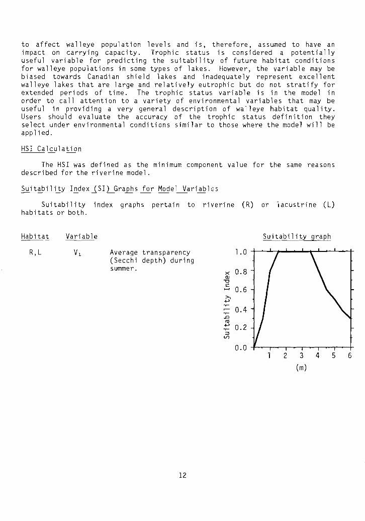
Habitat

R,L

Variable

Average transparency(Secchi depth) duringsummer.

12

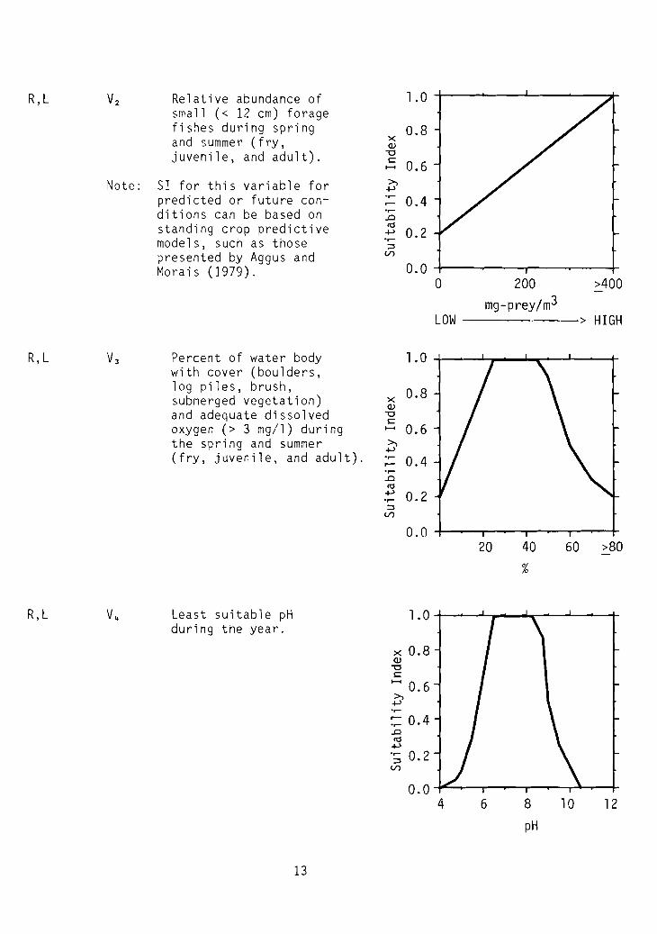
R,L Vz Relative abundance of 1.0small « 12 cm) foragefishes during spring 0.8and summer (fry, x

Q)

juvenile, and adult). -0s:: 0.6......

Note: SI for this variable for »+-'

predicted or future con- ......0.4

ditions can be based on ........0

standing crop predictive <t:l+-' 0.2

models, such as those ~

presented by Aggus and V')

Morais (1979). 0.00 200 >400

mg-prey/m3LOW > HIGH

R,L V3 Percent of water body 1.0with cover (boulders,log piles, brush, 0.8submerged vegetation) x

Q)

and adequate dissolved -0s::

oxygen (> 3 mg/l) during ...... 0.6the spring and summer »

+-'(fry, juvenile, and adult). ...... 0.4,...........

..0<t:l

+-' 0.2......~

V')

0.020 40 60 >80

%

R,L V4 Least suitable pH 1.0during the year.

x 0.8Q)-0s::

...... 0.6»+-'......:;: 0.4..0<t:l+-'.; 0.2V')

0.04 6 8 10 12

pH

13

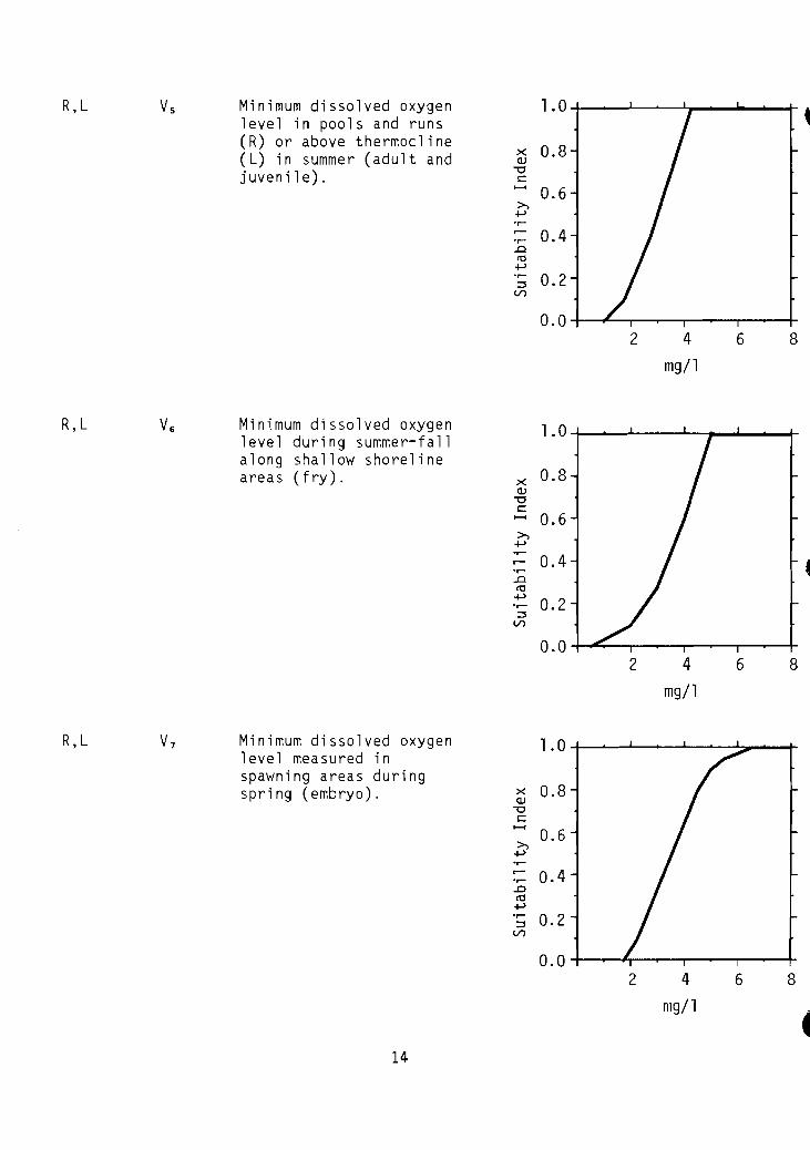
R,L Vs Minimum dissolved oxygen 1.0level in pools and runs( R) or above thermocline

0.8( L) in summer (adult and x(l)

juvenile). "'0c...... 0.6c-,

+.>......r- 0.4......oD<0+.>

::l 0.2Vl

0.02 4 6 8

mg/l

R,L V6 Minimum dissolved oxygen 1.0level during summer-fa 11along shallow shorelineareas (fry). x 0.8

(l)

"'0C...... 0.6c-,

+.>......0.4r-......

.a<0+.>

0.2......::lVl

0.02 4 6 8

mg/l

R,L V7 Minimum dissolved oxygen 1.0level measured inspawning areas duringspri ng (embryo). x 0.8

(l)

"'0C......

0.6c-,+.>............ 0.4oD<0

+.>...... 0.2::lVl

0.02 4 6 8

mg/l~

14

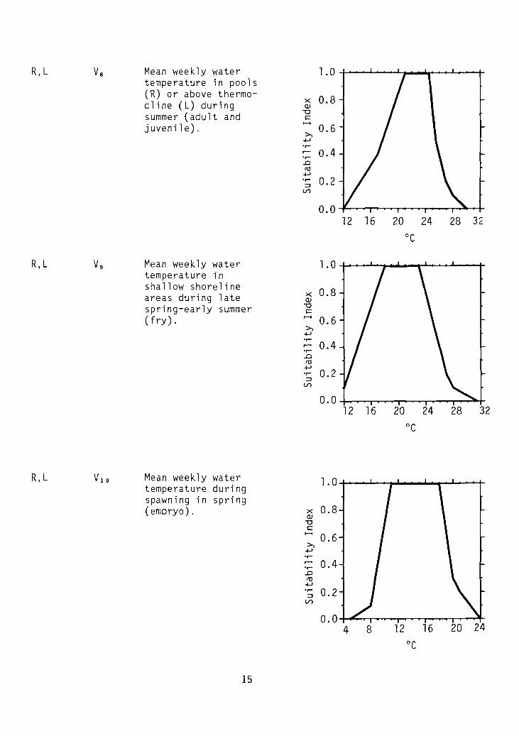
R,L Va Mean weekly water 1.0temperature in pools(R) or above thermo-

x 0.8cline (L) during <lJ

summer (adult and -0s::

juvenile).......

0.6>,+-'............ 0.4.0n::l+-'...... 0.2:::J(/)

0.012 16 20 24 28 32

°C

R,L Vg Mean weekly water 1.0temperature inshallow shoreline 0.8areas during late x

<lJ

spring-early summer -0s::

(fry) . ...... 0.6>,+-l......

0.4r--........cn::l+-'

0.2......:::J

(/)

0.012 16 20 24 28 32

°C

R,L VlD Mean weekly water 1.0temperature duringspawning in spring(embryo) . x 0.8

<lJ-0s::......

0.6>,+-'............ 0.4..cn::l+-l...... 0.2:::J(/)

0.04 8 12 16 20 24

°C

15

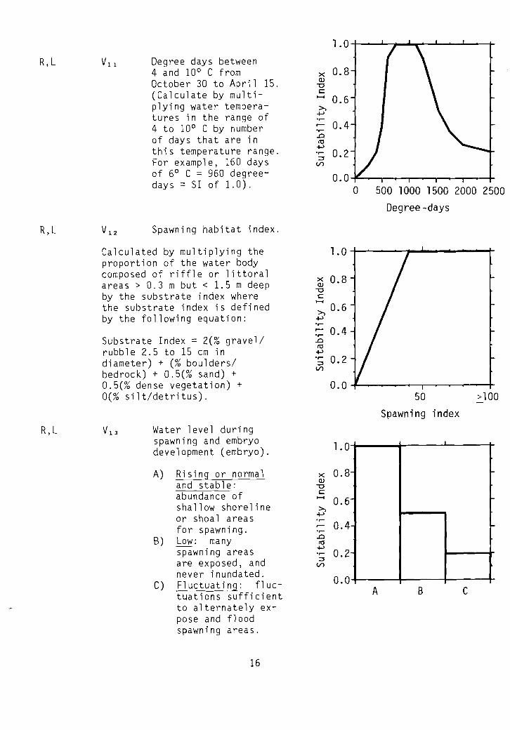
R,L

R,L

1.0

VII Degree days between4 and 10° C from x 0.8October 30 to April 15. (1)

-0

(Calculate by multi- t::...... 0.6plying water tempera- >,

tures in the range of ~......0.44 to 10° C by number ......

of days that are in .0~

this temperature range. ~...... 0.2For example, 160 days ~

(/)

of 6° C ~ 960 degree- 0.0days ~ SI of 1.0). 0 500 1000 1500 2000 2500

Degree -days

Spawning habitat index.

I

""

R,L

Calculated by multiplying theproportion of the water bodycomposed of riffle or littoralareas> 0.3 m but < 1.5 m deepby the substrate index wherethe substrate index is definedby the following equation:

Substrate Index ~ 2(% gravel/rubble 2.5 to 15 cm indiameter) + (% boulders/bedrock) + 0.5(% sand) +0.5(% dense vegetation) +0(% silt/detritus).

Water level duringspawning and embryodevelopment (embryo).

A) Rising or normaland stable:abundance ofshallow shorelineor shoal areasfor spawning.

B) Low: manyspawning areasare exposed, andnever inundated.

C) Fluctuating: fluc­tuations sufficientto alternately ex­pose and f1 oodspawning areas.

16

x 0.8(1)-0t::......>, 0.6~............ 0.4.0~

+>...... 0.2~

(/)

0.0

1.0

x 0.8(1)

-0t::...... 0.6>,+>......

0.4.......0~~

0.2......~

(/)

0.0A

50

Spawning index

B c

>100

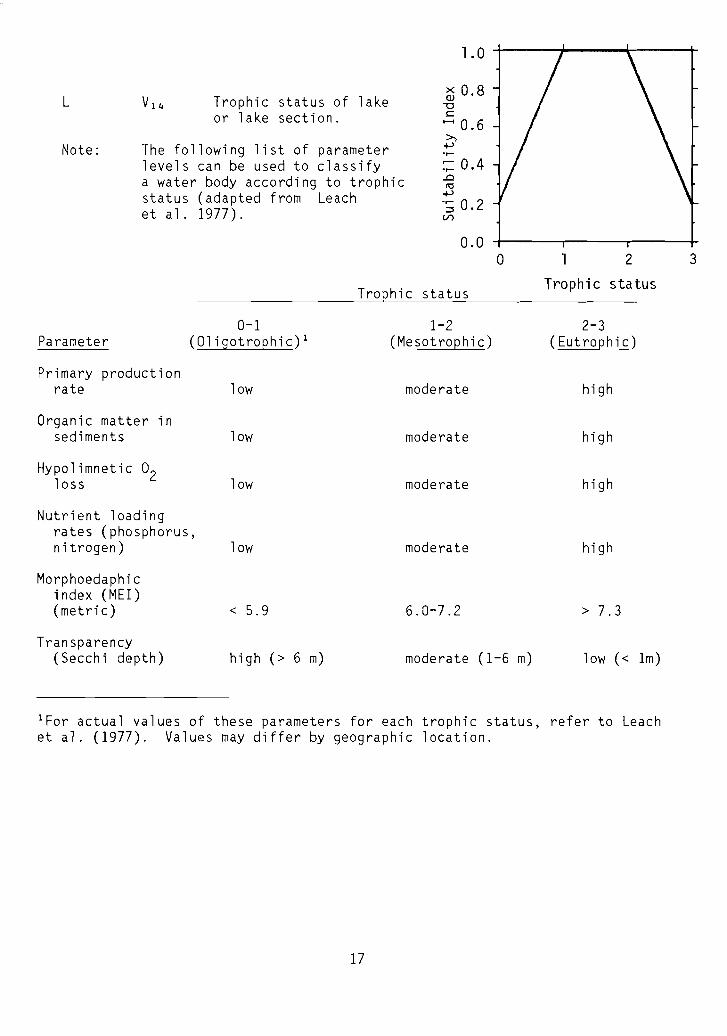
L

Note:

Vl 4 Trophic status of lakeor lake section.

The following list of parameterlevels can be used to classifya water body according to trophicstatus (adapted from Leachet al. 1977).

1.0

~ 0.8-0s:::

....... 0.6>,+-'

:;: 0.4..cro+-'0; 0.2(/')

0.0

0-1Parameter (Oligotrophic)l

Primary productionrate low

Organic matter insediments low

Hypolimnetic O2loss low

Trophic status

1-2(Mesotrophic)

moderate

moderate

moderate

o 2

Trophic status

2-3(Eutrophic)

high

high

high

3

Nutrient loadingrates (phosphorus,nitrogen)

Morphoedaphicindex (MEl)(metric)

Transparency(Secchi depth)

low

< 5.9

high (> 6 m)

moderate

6.0-7.2

moderate (1-6 m)

high

> 7.3

low « 1m)

lFor actual values of these parameters for each trophic status, refer to Leachet al. (1977). Values may differ by geographic location.

17

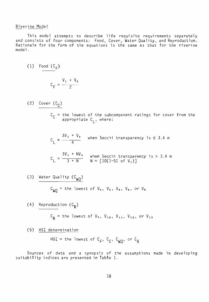
Riverine Model

This model attempts to describe life requisite requirements separatelyand consists of four components: Food, Cover, Water Quality, and Reproduction.Rationale for the form of the equations is the same as that for the riverinemode 1.

(2) Cover (CC)

Cc = the lowest of the subcomponent ratings for cover from theappropriate CL' where:

C = -----,,---L 4

(3) Water Quality (CWQ)

when Secchi transparency is ~ 3.4 m

when Secchi transparency is > 3.4 mN = [10(1-S1 of V1 ) ]

(4) Reproduction (CR)

(5) HS1 determination

HS1 = the lowest of CF' CC' CWQ' or CR

Sources of data and a synopsis of the assumptions made in developingsuitability indices are presented in Table 1.

18

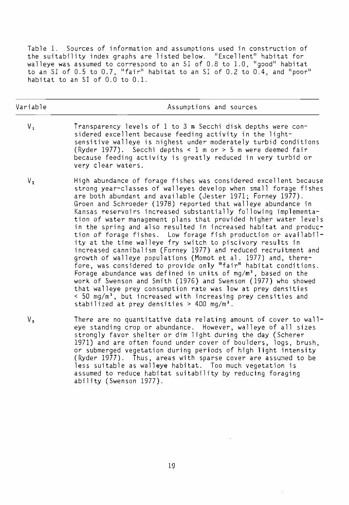
Table 1. Sources of information and assumptions used in construction ofthe suitability index graphs are listed below. "Excellent" habitat forwalleye was assumed to correspond to an SI of 0.8 to 1.0, "good" habitatto an .SI of 0.5 to 0.7, "fair" habitat to an SI of 0.2 to 0.4, and "poor"habitat to an SI of 0.0 to 0.1.

Variable Assumptions and sources

Transparency levels of 1 to 3 m Secchi disk depths were con­sidered excellent because feeding activity in the light­sensitive walleye is highest under moderately turbid conditions(Ryder 1977). Secchi depths < 1 m or > 5 m were deemed fairbecause feeding activity is greatly reduced in very turbid orvery clear waters.

High abundance of forage fishes was considered excellent becausestrong year-classes of walleyes develop when small forage fishesare both abundant and available (Jester 1971; Forney 1977).Groen and Schroeder (1978) reported that walleye abundance inKansas reservoirs increased substantially following implementa­tion of water management plans that provided higher water levelsin the spring and also resulted in increased habitat and produc­tion of forage fishes. Low forage fish production or availabil­ity at the time walleye fry switch to piscivory results inincreased cannibalism (Forney 1977) and reduced recruitment andgrowth of walleye populations (Momot et al. 1977) and, there­fore, was considered to provide only "fair ll habitat conditions.Forage abundance was defined in units of mg/m 3

, based on thework of Swenson and Smith (1976) and Swenson (1977) who showedthat walleye prey consumption rate was low at prey densities< 50 mg/m 3

, but increased with increasing prey densities andstabilized at prey densities> 400 mg/m 3

•

There are no quantitative data relating amount of cover to wall­eye standing crop or abundance. However, walleye of all sizesstrongly favor shelter or dim light during the day (Scherer1971) and are often found under cover of boulders, logs, brush,or submerged vegetation during periods of high light intensity(Ryder 1977). Thus, areas with sparse cover are assumed to beless suitable as walleye habitat. Too much vegetation isassumed to reduce habitat suitability by reducing foragingability (Swenson 1977).

19

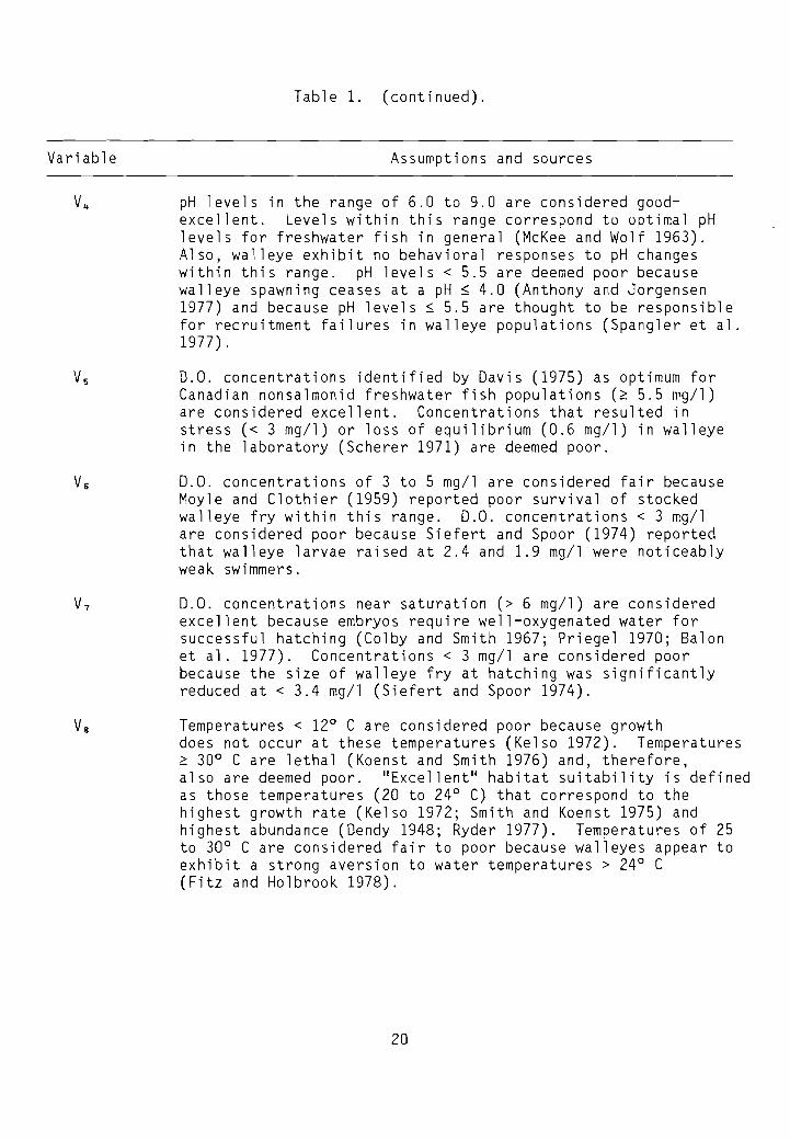
Table 1. (continued).

Variable Assumptions and sources

pH levels in the range of 6.0 to 9.0 are considered good­excellent. Levels within this range correspond to optimal pHlevels for freshwater fish in general (McKee and Wolf 1963).Also, walleye exhibit no behavioral responses to pH changeswithin this range. pH levels < 5.5 are deemed poor becausewalleye spawning ceases at a pH ~ 4.0 (Anthony and Jorgensen1977) and because pH levels ~ 5.5 are thought to be responsiblefor recruitment failures in walleye populations (Spangler et al.1977) .

D.O. concentrations identified by Davis (1975) as optimum forCanadian nonsalmonid freshwater fish populations (~ 5.5 mg/l)are considered excellent. Concentrations that resulted instress « 3 mg/l) or loss of equilibrium (0.6 mg/l) in walleyein the laboratory (Scherer 1971) are deemed poor.

D.O. concentrations of 3 to 5 mg/l are considered fair becauseMoyle and Clothier (1959) reported poor survival of stockedwalleye fry within this range. D.O. concentrations < 3 mg/lare considered poor because Siefert and Spoor (1974) reportedthat walleye larvae raised at 2.4 and 1.9 mg/l were noticeablyweak swimmers.

D.O. concentrations near saturation (> 6 mg/l) are consideredexcellent because embryos require well-oxygenated water forsuccessful hatching (Colby and Smith 1967; Priegel 1970; Balonet al. 1977). Concentrations < 3 mg/l are considered poorbecause the size of walleye fry at hatching was significantlyreduced at < 3.4 mg/l (Siefert and Spoor 1974).

Temperatures < 12° C are considered poor because growthdoes not occur at these temperatures (Kelso 1972). Temperatures~ 30° C are lethal (Koenst and Smith 1976) and, therefore,also are deemed poor. "Excellent" habitat suitability is definedas those temperatures (20 to 24° C) that correspond to thehighest growth rate (Kelso 1972; Smith and Koenst 1975) andhighest abundance (Dendy 1948; Ryder 1977). Temperatures of 25to 30° C are considered fair to poor because walleyes appear toexhibit a strong aversion to water temperatures> 24° C(Fitz and Holbrook 1978).

20

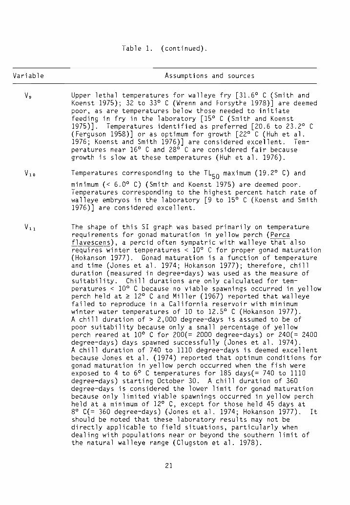
Table 1. (continued).

Variable Assumptions and sources

Upper lethal temperatures for walleye fry [31.6° C (Smith andKoenst 1975); 32 to 33° C (Wrenn and Forsythe 1978)J are deemedpoor, as are temperatures below those needed to initiatefeeding in fry in the laboratory [15° C (Smith and Koenst1975)J. Temperatures identified as preferred [20.6 to 23.2° C(Ferguson 1958)J or as optimum for growth [22° C (Huh et al.1976; Koenst and Smith 1976)J are considered excellent. Tem­peratures near 16° C and 28° C are considered fair becausegrowth is slow at these temperatures (Huh et al. 1976).

Temperatures corresponding to the TL50 maximum (19.2° C) and

minimum « 6.0° C) (Smith and Koenst 1975) are deemed poor.Temperatures corresponding to the highest percent hatch rate ofwalleye embryos in the laboratory [9 to 15° C (Koenst and Smith1976)J are considered excellent.

The shape of this SI graph was based primarily on temperaturerequirements for gonad maturation in yellow perch (Pereaflavescens), a percid often sympatric with walleye that alsorequires winter temperatures < 10° C for proper gonad maturation(Hokanson 1977). Gonad maturation is a function of temperatureand time (Jones et al. 1974; Hokanson 1977); therefore, chillduration (measured in degree-days) was used as the measure ofsuitability. Chill durations are only calculated for tem­peratures < 10° C because no viable spawnings occurred in yellowperch held at ~ 12° C and Miller (1967) reported that walleyefailed to reproduce in a California reservoir with minimumwinter water temperatures of 10 to 12.5° C (Hokanson 1977).A chill duration of > 2,000 degree-days is assumed to be ofpoor suitability because only a small percentage of yellowperch reared at 10° C for 200(= 2000 degree-days) or 240(= 2400degree-days) days spawned successfully (Jones et al. 1974).A chill duration of 740 to 1110 degree-days is deemed excellentbecause Jones et al. (1974) reported that optimum conditions forgonad maturation in yellow perch occurred when the fish wereexposed to 4 to 6° C temperatures for 185 days(= 740 to 1110degree-days) starting October 30. A chill duration of 360degree-days is considered the lower limit for gonad maturationbecause only limited viable spawnings occurred in yellow perchheld at a minimum of 12° C, except for those held 45 days at8° C(= 360 degree-days) (Jones et al. 1974; Hokanson 1977). Itshould be noted that these laboratory results may not bedirectly applicable to field situations, particularly whendealing with populations near or beyond the southern limit ofthe natural walleye range (Clugston et al. 1978).

21

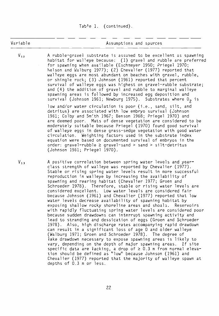
Table 1. (continued).

Variable Assumptions and spurces

A rubble-gravel substrate is assumed to be excellent as spawninghabitat for walleye because: (1) gravel and rubble are preferredfor spawning when available (Eschmeyer 1950; Priegel 1970;Nelson and Walburg 1977); (2) Chevalier (1977) reported thatwalleye eggs are most abundant on beaches with gravel, rubble,or shingle rock; (3) Johnson (1961) reported that percentsurvival of walleye eggs was highest on gravel-rubble substrate;and (4) the addition of gravel and rubble to marginal walleyespawning areas is followed by increased egg deposition andsurvival (Johnson 1961; Newburg 1975). Substrates where O2 is

low and/or water circulation is poor (i .e., sand, silt, anddetritus) are associated with low embryo survival (Johnson1961; Colby and Smith 1967; Benson 1968; Priegel 1970) andare deemed poor. Mats of dense vegetation are considered to bemoderately suitable because Priegel (1970) found good survivalof walleye eggs in dense grass-sedge vegetation with good watercirculation. Weighting factors used in the substrate indexequation were based on documented survival of embryos in theorder: gravel-rubble ~ gravel-sand> sand> silt-detritus(Johnson 1961; Priegel 1970).

A positive correlation between spring water levels and year­class strength of walleye was reported by Chevalier (1977).Stable or rising spring water levels result in more successfulreproduction in walleye by increasing the availability ofspawning and rearing habitat (Chevalier 1977; Groen andSchroeder 1978). Therefore, stable or rising water levels areconsidered excellent. Low water levels are considered fairbecause Johnson (1961) and Chevalier (1977) reported that lowwater levels decrease availability of spawning habitat byexposing shallow rocky shoreline areas and shoals. Reservoirswith rapidly fluctuating spring water levels are considered poorbecause sudden drawdowns can interrupt spawning activity andlead to stranding and dessication of eggs (Groen and Schroeder1978). Also, high discharge rates accompanying rapid drawdowncan result in a significant loss of age 0 and older walleye(Walburg 1971; Groen and Schroeder 1978). The degree oflake drawdown necessary to expose spawning areas is likely tovary, depending on the depth of major spawning areas. If sitespecific data are lacking, a drop of ~ 0.3 m from normal eleva­tion should be defined as 11 0 W" because Johnson (1961) andChevalier (1977) reported that the majority of walleye spawn atdepths of 0.3 m or less.

22

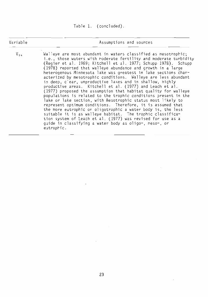
Table 1. (concluded).

Variable Assumptions and sources

Walleye are most abundant in waters classified as mesotrophic;i.e., those waters with moderate fertility and moderate turbidity(Regier et al. 1969; Kitchell et al. 1977; Schupp 1978). Schupp(1978) reported that walleye abundance and growth in a largeheterogenous Minnesota lake was greatest in lake sections char­acterized by mesotrophic conditions. Walleye are less abundantin deep, clear, unproductive lakes and in shallow, highlyproductive areas. Kitchell et al. (1977) and Leach et al.(1977) proposed the assumption that habitat quality for walleyepopulations is related to the trophic conditions present in thelake or lake section, with mesotrophic status most likely torepresent optimum conditions. Therefore, it is assumed thatthe more eutrophic or oligotrophic a water body is, the lesssuitable it is as walleye habitat. The trophic classifica-tion system of Leach et al. (1977) was revised for use as aguide in classifying a water body as oligo-, meso-, oreutrophic.

23

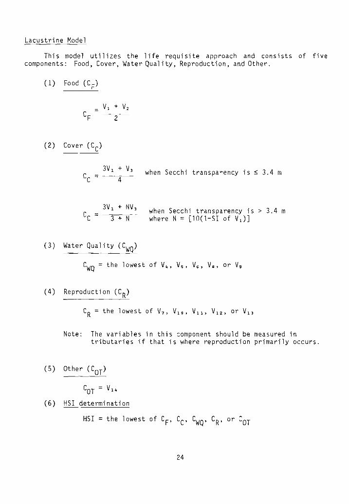
Lacustrine Model

This model utilizes the life requisite approach and consists of fivecomponents: Food, Cover, Water Quality, Reproduction, and Other.

(2) Cover (CC)

when Secchi transparency is ~ 3.4 m

when Secchi transparency is > 3.4 mwhere N = [10(1-SI of V1 ) ]

(3) Water Quality (CWQ)

(4) Reproduction (C R)

Note: The variables in this component should be measured intributaries if that is where reproduction primarily occurs.

(5) Other (COT)

COT = V1 4

(6) HSI determination

HSI = the lowest of CF' CC' CWQ' CR' or COT

24

Sources of data and assumptions made in developing the suitability indicesare presented in Table 1.

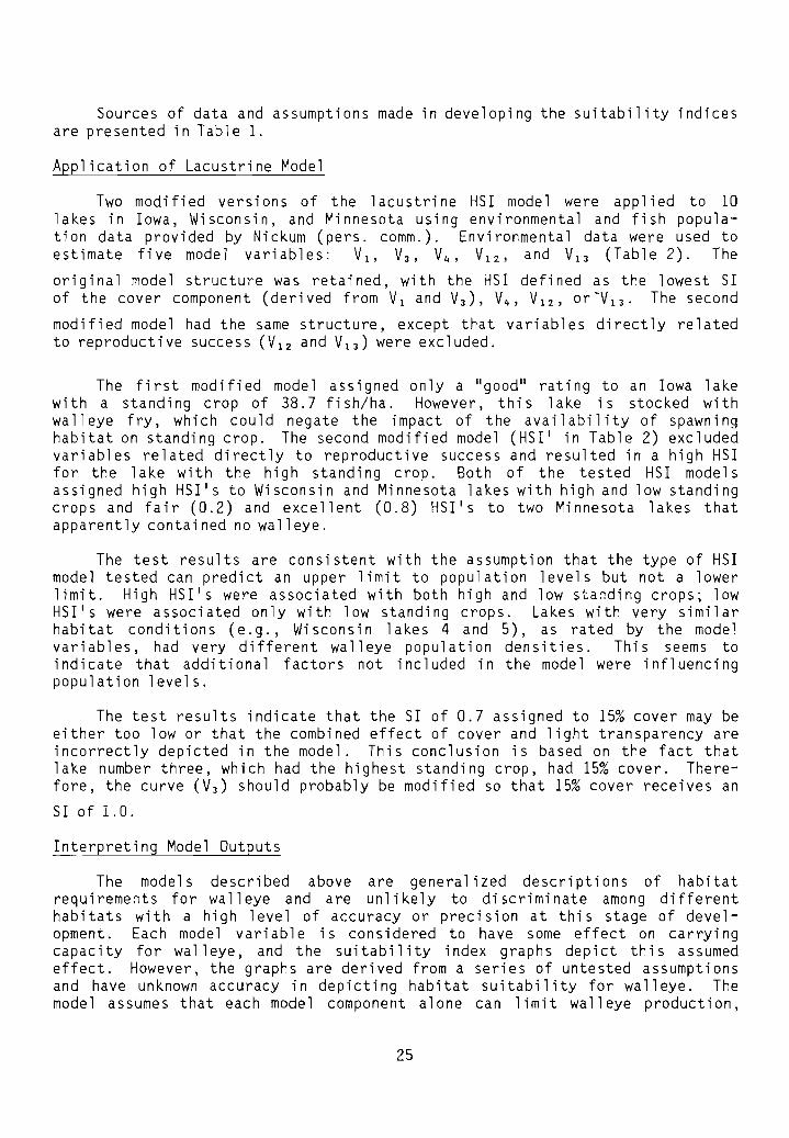
Application of Lacustrine Model

Two modified versions of the lacustrine HSI model were appl ied to 10lakes in Iowa, Wisconsin, and Minnesota using environmental and fish popula­tion data provided by Nickum (pers. comm.). Environmental data were used toestimate five model variables: V1 , VJ , V4 , V1 2 , and V13 (Table 2). The

original model structure was retained, with the HSI defined as the lowest SIof the cover component (derived from V1 and VJ ) , V4 , V1 2 , or-V 1 J • The second

modified model had the same structure, except that variables directly relatedto reproductive success (V1 2 and V1 J ) were excluded.

The first modified model assigned only a "qcod" rating to an Iowa lakewith a standing crop of 38.7 fish/ha. However, this lake is stocked withwalleye fry, which could negate the impact of the availability of spawninghabitat on standing crop. The second modified model (HSI ' in Table 2) excludedvariables related directly to reproductive success and resulted in a high HSIfor the lake with the high standing crop. Both of the tested HSI model sassigned high HSI's to Wisconsin and Minnesota lakes with high and low standingcrops and fair (0.2) and excellent (0.8) HSI's to two Minnesota lakes thatapparently contained no walleye.

The test results are consistent with the assumption that the type of HSImodel tested can predict an upper limit to population levels but not a lowerlimit. High HSI's were associated with both high and low standing crops; lowHSI's were associated only with low standing crops. Lakes with very similarhabitat conditions (e.g., Wisconsin lakes 4 and 5), as rated by the mode ]variables, had very different walleye population densities. This seems toindicate that additional factors not included in the model were influencingpopulation levels.

The test results indicate that the SI of 0.7 assigned to 15% cover may beeither too low or that the combined effect of cover and light transparency areincorrectly depicted in the model. This conclusion is based on the fact thatlake number three, which had the highest standing crop, had 15% cover. There­fore, the curve (VJ ) should probably be modified so that 15% cover receives an

SI of 1.0.

Interpreting Model Outputs

The models described above are generalized descriptions of habitatrequirements for walleye and are unlikely to discriminate among differenthabitats with a high level of accuracy or precision at this stage of devel­opment. Each model variable is considered to have some effect on carryingcapacity for walleye, and the suitability index graphs depict this assumedeffect. However, the graphs are derived from a series of untested assumptionsand have unknown accuracy in depicting habitat suitability for walleye. Themodel assumes that each model component alone can limit walleye production,

25

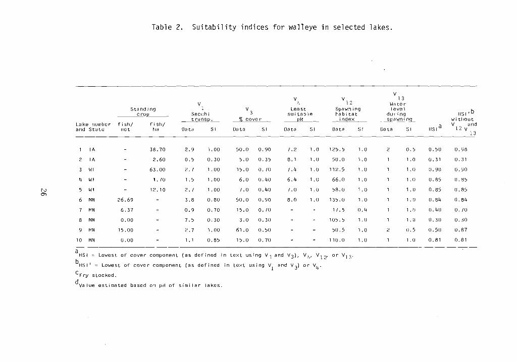
Table 2. Suitability indices for walleye in selected lakes.

vv V 1 3

V 4 12 WaterStanding 1 V

3Lea s t Spawning level

HSI' bcrop Secchi sUitable habitat du ringtransp. % cove r pH index _----.i.Pawn ill~ without

La ke number fish/ fish/HS,a

V andand State net ha Dat a SI Dat a SI Dat a SI Data SI Data SI 12 V

13

IA - 38.70 2.9 1. 00 50.0 0.90 7.2 1.0 125.5 1.0 2 0.5 0.50 0.98

2 IA - 2.60 0.5 0.30 5.0 0.35 8.1 1.0 50.0 1.0 1 1 .0 0.31 0.31

3 WI - 63.00 2.7 1. 00 15.0 0.70 7.4 1.0 112.5 1.0 1 1 . 0 0.90 0.90

4 WI - 1.70 1.5 1. 00 6.0 0.40 6.4 1.0 66.0 1.0 1 1.0 0.85 0.85

rv 5 WI - 12.10 2.7 1.00 7.0 0.40 7.0 1.0 58.0 1.0 1 1.0 0.85 0.85O'l

6 MN 26.69 - 3.8 0.80 50.0 0.90 8.0 1.0 135.0 1.0 1 1.0 0.84 0.81j

7 MN 6.37 - 0.9 0.70 15.0 0.70 - - 17.5 0.4 1 1 . f) 0.40 0.70

8 MN 0.00 - 7.5 0.30 3.0 0.30 - - 105.5 1.0 1 1.0 0.30 0.30

9 t~N 15.00 - 2.7 1.00 61.0 0.50 - - 50.5 1.0 2 0.5 0.50 0.87

10 MN 0.00 - 1.1 0.85 15.0 0.70 - - 110.0 1.0 1 1 .0 0.81 0.81

a .in text using VI and V3)' V4' V I 2' or V13 .HSI ~ Lowest of cover component (as defined

bHS 1' ~ Lowest of cover component (as defined in text using VI and V3)

or V4.

CFry stocked.

dvalue estimated based on pH of similar lakes.

but this has not been tested. A major weakness of the models is that, whilemodel variables may be necessary to determine the suitability of habitat forwall~ye, they may not be sufficient. Therefore, high HSI's may be associatedwith low or zero standing crops, as well as high standing crops. It should beremembered that lakes unsuitable for walleye reproduction may support a walleyefishery through supplemental stocking with fry.

Model outputs should be interpreted as indicators (or predictors) ofexcellent (0.8 to 1.0), good (0.5 to 0.7), fair (0.2 to 0.4), or poor (0.0 to0.1) habitat for walleye. The output of the model s provided should be mostuseful in comparing different habitats. If two study areas have differentHSI's, the one with the higher HSI is expected to have the potential to supporta larger walleye population. The models also provide the basic framework forincorporating new model hypotheses or other site-specific factors that affecthabitat suitability for walleye. Users should recognize that carrying capacityis a concept not a measurable response for which one can build a falsifiablepredictive model. Users conducting impact assessments r equt r l no major modelimprovements and testing should concentrate on building a falsifiable model.The model should use a clearly documented chain of logic to predict a measur­able response (e.g., growth) that is acceptable for judging a selected impact.

ADDITIONAL HABITAT MODELS

Mode 1 1

Where water quality is not limiting, optimum riverine habitat for walleyeis characterized by the following conditions: moderate-to-large river size;cool temperatures (average summer temperature from 20 to 24° C; winter tem­peratures < 10° C); mesotrophic conditions; high abundance of rocky shoal andshoreline areas for spawning; and high abundance of small forage fishes:

HSI = number of above criteria present5

Model 2

Where water quality is not 1imit i ng, optimum 1acustri ne habi tat forwalleye is characterized by the following conditions: moderate-to-large lakesize (> 100 ha); cool temperatures (as in Modell above); mesotrophic condi­tions; abundance of rocky shoal and shoreline areas for spawning; and highabundance of small forage fishes:

HSI = number of above criteria present5

27

Model 3

Aggus and Morais (1979) and Aggus and Bivin (1982) developed regressionequations relating walleye standing crop or harvest in reservoirs to easilymeasured environmental variables. These authors discuss procedures for usingthe equations, as well as limitations of the models.

Model 4

Prentice and Clark (1978) presented a walleye population dynamics model(WALLEYE) for predicting walleye stocking success based on reservoir habitatconditions and predator abundance. The model was developed from data on 17Texas reservoirs. Model simulations showed good agreement with actual walleyepopulation abundance data. WALLEYE can provide information on potentialsuccess of walleye introductions and evaluate the need for, and success of,habitat improvements.

INSTREAM FLOW INCREMENTAL METHODOLOGY (IFIM)

The U.S. Fish and Wildlife Service's Instream Flow Incremental Methodology(IFIM), as outlined by Bovee (1982), is a set of ideas used to assess instreamflow problems. The Physical Habitat Simulation System (PHABSIM), described byMilhous et al. 1981, is one component of the IFIM that can be used byinvestigators interested in determining the amount of available instreamhabitat for a fish species as a function of streamflow. The output generatedby PHABSIM can be used for several IFIM habitat display and interpretationtechniques, including:

1. Optimization. Determination of monthly flows that minimize habitatreductions for species and life stages of interest;

2. Habitat Time Series. Determination of the impact of a project onhabitat by imposing project operation curves over historical flowrecords and integrating the difference between the curves; and

3. Effective Habitat Time Series. Calculation of the habitat require­ments of each life stage of a fish species at a giv8n time by usinghabitat ratios (relative spatial requirements of various lifestages).

Suitability Index Graphs as Used in IFIM

PHABSIM utilizes Suitability Index graphs (SI curves) that describe theinstream suitability of the habitat variables most closely related to streamhydraulics and channel structure (velocity, depth, substrate, temperature, andcover) for each major life stage (spawning, egg incubation, fry, juvenile, andadult) of a given fish species. The specific curves required for a PHABSIManalysis represent the hydraulic-related parameters for which a species orlife stage demonstrates a strong preference (i .e., a pelagic species that onlyshows preferences for velocity and temperature will have very broad curves for

28

depth, substrate, and cover). Instream Flow Information Papers 11 (Milhouset al. 1981) and 12 (Bovee 1982) should be reviewed carefully before using anycurves for a PHAB5IM analysis. 51 curves used with the IFIM that are generatedfrom empirical microhabitat data are quite similar in appearance to the moregenera 1i zed 1i terature-based 51 curves developed in many H5I mode 1s (Armouret al. 1983). These two types of 51 curves are interchangeable, in somecases, after conversion to the same units of measurement (English, metric, orcodes).

51 curve validity is dependent on the quality and quantity of informationused to generate the curve. The curves used need to accurately reflect theconditions and assumptions inherent to the model(s) used to aggregate thecurve-generated 5I 's into a measure of habitat suitability. If the necessarycurves are unavailable or if available curves are inadequate (i.e., built ondifferent assumptions), a new set of curves should be generated (data collec­tion and analyses techniques for curve generation will be included in a forth­coming Instream Flow Information Paper).

There are several ways to develop 51 curves. The method selected dependson the habitat model that will be used and the available database for thespecies. The validity of the curve is not obvious and, therefore, the methodby which the curve is generated and the qual ity of the database are veryimportant. Care al so must be taken to choose the habitat model most appro­priate for the specific study or evaluation; the choice of models determinesthe type of 51 curves that will be used. For example, in an H5I model, a 51curve for velocity usually reflects suitability of average channel (stream)velocity (i.e., a macrohabitat descriptor); in an IFIM analysis, 51 curves forvelocity are assumed to represent suitability of the velocity at the point inthe stream occupied by a fish (i .e., a microhabitat descriptor) (Armour et al.1983).

A system with standard terminology has been developed for classifying 51curve sets and describing the database used to construct the curves in IFIMapplications. The classification is not intended to define the quality of thedata or the accuracy of the curves. There are four categories in the classifi­cation. A literature-based (category one) curve is a generalized descriptionor summary of habitat preferences based data found in the literature. Thistype of curve usually is based on information in published references on theupper and lower limits of a variable for a species (e.g., juveniles are usuallyfound at water depths of 0.3 to 1.0 m). Unpublished data and expert opinionalso can be used to develop these curves. Occasionally, the reference alsocontains information on the optimum or preferred condition within the limitsof tolerance (e.g., juveniles are found at water depths of 0.3 to 1.0 m, butare most common at depths from 0.4 to 0.6 m). Vi rtua lly a11 of the 51 curvespublished in the H5I series for depth, velocity, and substrate, are categoryone curves.

Utilization curves (category two) are based on a frequency analysis offish observations in the stream environment with the habitat variables measuredat each sighting [see Instream Flow Information Paper 3 (Bovee and Cochnauer1977) and Instream Flow Information Paper 12 (Bovee 1982:173-196)J. These

29

curves are designated as utilization curves because they depict the habitatconditions a fish will use within a specific range of available conditions.Because of the way the data are collected for utilization curves, the resultingfunction represents the probability of occurrence of a particular environmentalcondition, given the presence of a fish of a particular species, P(EI F).Utilization curves are generally more precise for IFIM applications thanliterature-based curves because they are based on specific measurements ofhabi tat cha racteri st i cs where the fi sh actually occur. However, ut i 1i zat ioncurves may not be transferable to streams that differ substantially in sizeand complexity from the streams where the data were obtained.

A preference curve (category three) is a utilization curve that has beencorrected for envi ronmenta 1 bi as. For examp 1e, if 50% of the fi sh are foundin pools over 1.0 m deep, but only 10% of the stream has such pools, the fishare actively selecting that type of habitat. Preference curves approximatethe function of the probability of occurrence of a fish, given a set of envi­ronmental conditions:

P(FIE) := P(EIF)peE)

Only a limited number of experimental data sets have been compiled intoIFIM preference curves. The development of these curves should be the goal ofall new curve development efforts.

The fourth category of curves is still largely conceptual. One type ofcurve under consideration is a cover-conditioned, or season-conditioned,preference curve set. Such a curve set woul d con si st of di fferent depth­velocity preference curves as a function or condition of the type of coverpresent or the time of year. No fourth category curves have been developed atthis time.

The advantage of category three and four curves is the sign i fi cantimprovement in precision and confidence in the curves when applied to streamssimilar to the streams where the original data were obtained. The degree ofincreased accuracy and transferability obtainable when applying these curvesto dissimilar streams is unknown. In theory, the curves should be widelytransferable to any stream in which the environmental conditions are withinthe range of conditions found in the streams for which the curves weredeveloped.

Availability of Graphs for Use in IFIM

Table 3 lists the SI curves available for an IFIM analysis of walleyehabitat. All curves should be reviewed before use to determine applicability.

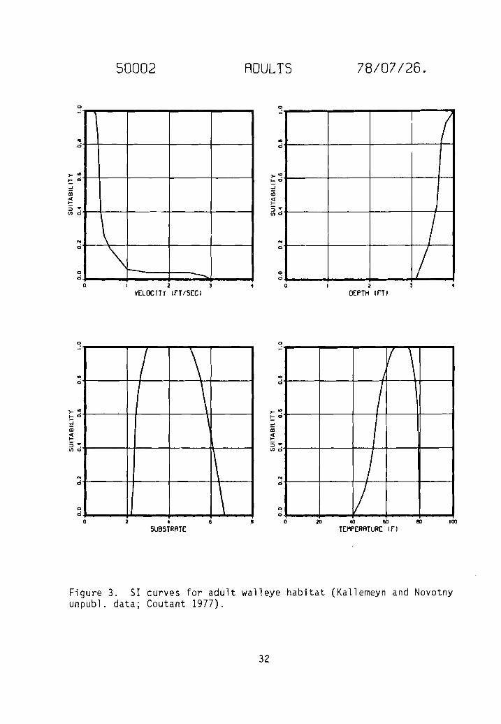
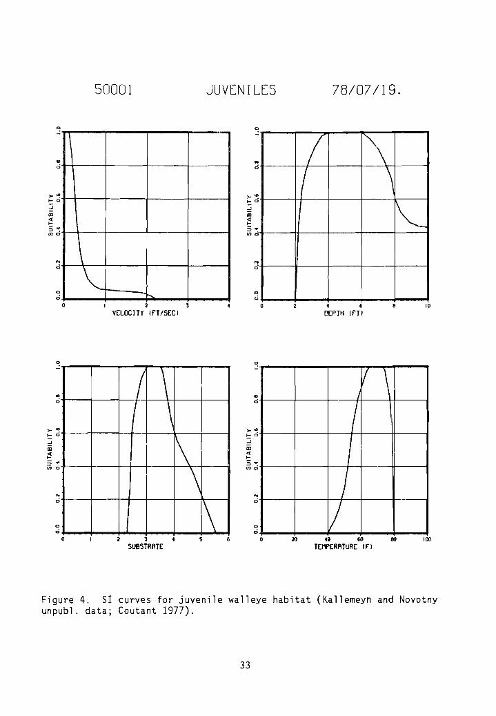
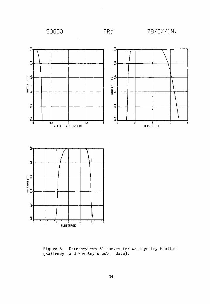
Category two 51 curves for adult velocity and substrate (Fig. 3), juvenilevelocity, depth, and substrate (Fig. 4), and fry velocity, depth, and substrate(Fig. 5) were generated as a result of frequency analyses of raw data collected

30

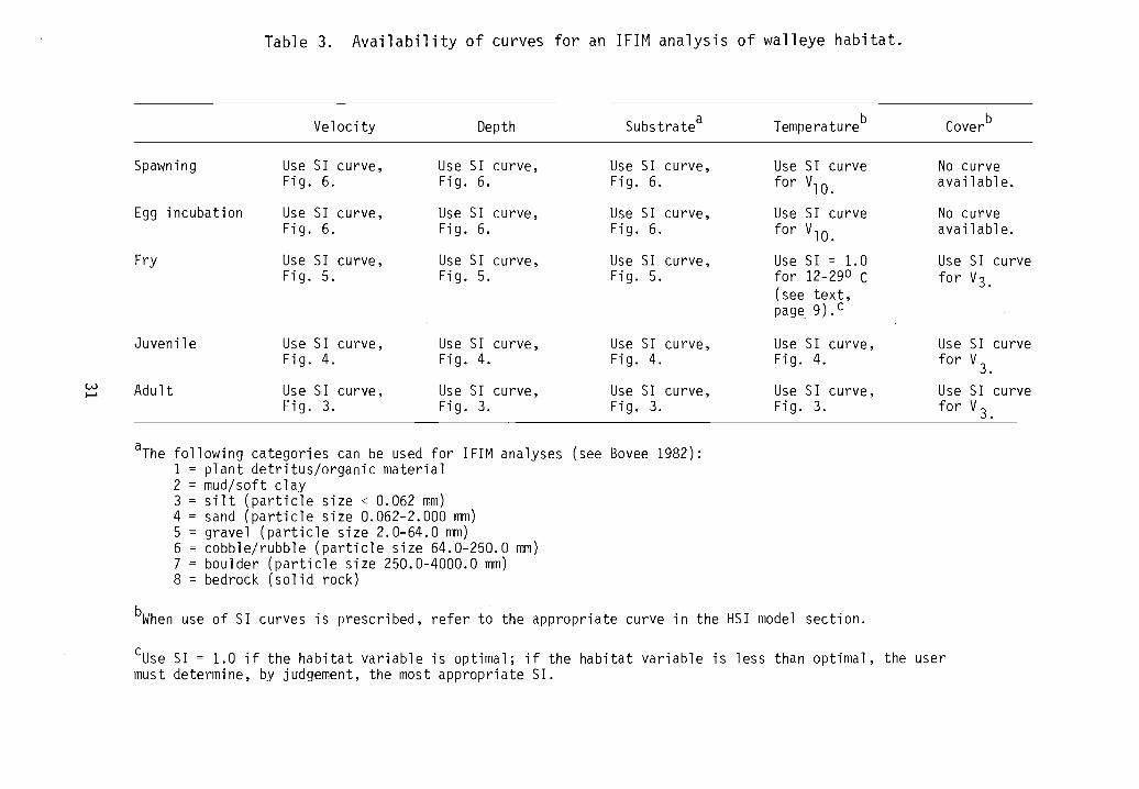
Table 3. Availability of curves for an IFIM analysis of walleye habitat.

Velocity Depth SUbstratea Temperatureb Coverb

Spawning Use S1 curve, Use S1 curve, Use S1 curve, Use S1 curve No curveFig. 6. Fig. 6. Fig. 6. for V10. available.

Egg incubation Use S1 curve, Use S1 curve, Use S1 curve, Use S1 curve No curveFig. 6. Fig. 6. Fig. 6. for V10. available.

Fry Use S1 curve, Use S1 curve, Use S1 curve, Use S1 = 1. 0 Use S1 curveFig. 5. Fig. 5. Fig. 5. for 12-290 C for V3.

(see text,page 9).c

Juvenile Use S1 curve, Use S1 curve,Fig. 4. Fig. 4.

w Adult Use SI curve, Use S1 curve,.......Fig. 3. Fig. 3.

Use S1 curve,Fig. 4.

Use S1 curve,Fig. 3.

Use S1 curve,Fig. 4.

Use S1 curve,Fig. 3.

Use S1 curvefor V3.

Use S1 curvefor V3.

aThe following categories can be used for 1F1M analyses (see Bovee 1982):1 = plant detritus/organic material2 = mud/soft clay3 = silt (particle size < 0.062 mm)4 = sand (particle size 0.062-2.000 mm)5 = gravel (particle size 2.0-64.0 mm)6 = cobble/rubble (particle size 64.0-250.0 mm)7 = boulder (particle size 250.0-4000.0 mm)8 = bedrock (solid rock)

bWhen use of S1 curves is prescribed, refer to the appropriate curve in the HS1 model section.

cUse S1 = 1.0 if the habitat variable is optimal; if the habitat variable is less than optimal, the usermust determine, by judgement, the most appropriate S1.

a

50002 ADULTS

a

78/07/26.

\-,I-- -- o

coo

>- '"I- 0-J

III

~:3 ...VI 0

...o

ao

a

o 2

vELOCITY 1fT/SEC)

coa

...o

ao

a

/

I7

2DEPTH IfTJ

! \\\

\

\

II \I

I

1p

coa

>-'"~a

-J

III

~3'"VIa

...a

aa

o 2 4

SUBSTRRTE6 I

coa

>-'"1-0....III

~S ...VIa

...o

aa

o 20 40 60

TEMPERRTURE Ir:10 100

Figure 3. 51 curves for adult walleye habitat (Kallemeyn and Novotnyunpubl. data; Coutant 1977).

32

o

50001 JUVENILES

o

78/07/19.

\

\~

-"o

I \I \

~

'"ci

>-~1-0

-'aI

;:!3"m";

N

.,;

o.,;

o

o 2 ]VELOCITY (fT/SEC)

'".,;

>-~1- 0

:::!aI

;:!3·m";

N

ci

oci

o

4 6DEPTH trr,

8 10

( \I \

\\\

/ \I

II

//

--

'"e

>- ~1-0

-'aI

;:!3~m 0

...

.,;

o.,;

o 2 ]SUBSTRATE

5 6

CD

.,;

>-<Dt::: ci-'aI<OfI-

3·me

...e

oci

o 20 4g 60

TEMPERATURE I rJ80 100

Figure 4. 51 curves for juvenile walleye habitat (Kallemeyn and Novotnyunpubl. data; Coutant 1977).

33

\ ---- -------

7 \\

l\

\\\

/ \I

._-

I

o

'"ci

N

ci

oc:i

o

'"c:i

>-'"t: ci-'iii;=S·lJ)0

N

ci

oc:i

o

o

50000

0.5 I 1.5VELOCITY (fT/SECI

3SUBSTRATE

FRY

o

.,ci

'">--... 0

-'al<fl::.::J"lJ)0

N

ci

oci

6

o 2

78/07/19.

1

DEPTH 1fT)8

Figure 5. Category two 51 curves for walleye fry habitat(Kallemeyn and Novotny unpubl. data).

34

by Kallemeyn and Novotny (unpubl. data). Kallemeyn and Novotny sampled theMissouri River at each of four stations for 4 days every 4 weeks from 29 Marchto 4 November 1976. Three stations were on unchannelized sections of riverlocated on the South Dakota/Nebraska border, one be low the Fort Renda11 Damand two below the Gavins Point Dam. The fourth station was on a channelizedsection of river on the Iowa/Nebraska border below Sioux City. Sampling gearincluded gill nets, trammel nets, hoop nets, seines, a drop trap, an electro­shocker, and plankton nets. A total of 20 fry, 48 juveniles, and 41 adultwalleye were collected and the data used in frequency analyses.

Habitat types identified in the unchannelized sections of the MissouriRiver included main channel, main channel border, sandbar, chute, backwater,pool, and marsh; those in channelized sections of the river included mainchannel, spur dike, notched spur dike, notched wing dike, revetment, andnotched revetment. During the study, channel widths ranged from 300 to 1,500 m(x = 640 to 760 m), depths ranged from 0.0 to 8.0 m (x < 2.0 m), da ily meandischarges ranged from 872 to 1,104 m3/sec' (x ~ 1,105 m3/sec), surface veloci­ties ranged from 0.0 to 2.1 m/sec, the gradient was approximately 0.2 m/km,surface water temperatures ranged from 3.5 to 27.5° C, turbidity ranged from2.3 to 33.0 JTU's, and conductivity ranged from 550 to 780 urnho sz' cm. Thesubstrate consisted primarily of sand, but silt was dominant in backwater andmarsh areas.

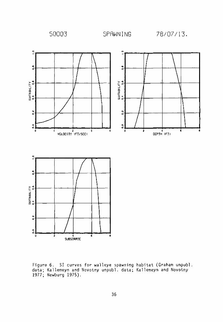
The category two SI curve for spawning velocity (Fig. 6) was generatedfrom a frequency analysis of raw data (Graham unpubl. data) collected frombelow the intake diversion (river mile 71.1) on the Yellowstone River inMontana from 18 Apri 1 to 6 May 1977. A tota 1 of 230 eggs were co 11 ected atnight from four transects located on a 3/4 mile gravel bar. Collections weremade using a 20-inch square net for kick sampling. During the study, flowsranged from 5,900 to 10,600 CFS, velocities sampled ranged from 0.7 to 3.9 fps,depths sampled ranged from 1 to 3 ft, substrate observed was predominantlygravel and cobble with some sand, and temperatures ranged from 52 to 53° F.

The category two SI curve for spawning depth (Fig. 6) was derived fromfrequency analyses of the raw data collected by Graham (unpubl. data) and thedata collected by Kallemeyn and Novotny (unpubl. data). The SI curve forspawning substrate (Fig. 6) is a category one curve and was generated as aresult of information obtained from Graham's unpublished data and articlespublished by Kallemeyn and Novotny (1977), and Newburg (1975). The categoryone curve for adult temperature preferences (Fig. 2) was derived from informa­tion in a publication by Coutant (1977); the assumption was made that juvenilewalleye prefer the same temperatures as adults.

The SI curve for adult walleye depth utilization (Fig. 2) was generatedfrom a frequency analysis of the data collected by Kallemeyn and Novotny(unpubl. data) and data collected by Russell (unpubl. data). Russell usedscuba diving to observe walleye adults in 36 pools within 39 mi of the CurrentRiver, between Van Buren and Doniphan in Carter and Ripley counties ofMissouri, during 6 days in 1970 and 1971. Approximately 613 walleye wereobserved, wei ghi ng from 1 to 10 1bs. Pool 1engths ranged from 75 to 450 ft,

35

50003 SPAWNING 78/07/13.

o o

/ ~I \

V \J

/i.>

v

o

/ \\,

I 1\

I 1\

/6•DEPTH IfTl

2

'"o

Cl

o

oo

2VELOCITY 1fT/SEC)

o

oo

'"o

Cl

o

>-~1- 0

..J

III4t.~.

1Jl0

o

( \( \

II

//

Cl

o

>-'"1-0..JIII

~5·lJlo

'"o

oo

o 2 •sueSTRATE6 8

Figure 6. SI curves for walleye spawning habitat (Graham unpubl.data; Kallemeyn and Novotny unpubl. data; Kallemeyn and Novotny1977; Newburg 1975).

36

and maximum pool depths ranged from 8 to 18 ft. Walleye congregated in poolsduring the day and moved into the shallows to feed at night in these sampleareas. Therefore, users of the SI curve for adult depth utilization should beaware that the curve represents daytime resting habitat.

REFERENCES

Aggus, L. R., and D. 1. Morais. 1979. Habitat suitability index equationsfor reservoi rs based on standi ng crop of fi sh. Nat 1. Reservoi r Res.Prog. Rep. to U.S. Fish Wildl. Servo 120 pp.

Aggus, L. R., and W. M. Bivin. 1982. Habitat suitability index models:Regression models based on harvest of coolwater and coldwater fishes inreservoirs. U.S. Fish Wildl. Servo FWS/OBS-82/10.25. 38 pp.

Ali, M. A., R. A. Ryder, and M. Anctil. 1977. Photoreceptors and visual pig­ments as related to behavioral responses and preferred habitats of perches(Perea spp.) and pikeperches (Stizostedion spp.). J. Fish. Res. BoardC~34(10):1475-1480.

Anthony, D. D., and C. R. Jorgensen. 1977. Factors in the declining contrib­utions of walleye (Stizostedion vitreum vitreum) to the fishery of LakeNipissing, Ontario 1960-76. J. Fish. Res. Board Can. 34(10):1703-1709.

Armour, C. L., R. J. Fisher, and J. W. Terrell. 1983. Comparison andrecommendations for use of Habitat Evaluation Procedures (HEP) and theInstream Flow 1ncremental Methodology (IFIM) for aquatic analyses. Draftrep. U.S. Fish Wildl. Serv., Western Energy and Land Use Team, FortCollins, CO. 42 pp.

Balon, E. K., W. T. Momot, and H. A. Regier. 1977. Reproductive guilds ofpercids: results of the paleogeographical history and ecological succes-sion. J. Fish. Res. Board Can. 34(10):1910-1921.

Benson, N. G.reservoirs.

1968. Revi ew of fi shery studi es on Mi ssouriU.S. Fish Wildl. Servo Res. Rep. 71. 61 pp.

main stem

Bovee, K. D. 1982. A guide to stream habitat analysis using the InstreamFlow Incremental Methodology. Instream Flow Information Paper 12. U.S.Fish Wildl. Servo FWS/OBS-82/26. 248 pp.

Bovee, K. D., and T. Cochnauer. 1977. Development and evaluation of weightedcriteria, probability-of-use curves for instream flow assessments:fisheries. Instream Flow Information Paper 3. U.S. Fish Wildl. ServoFWS/OBS-77/63. 39 pp.

Bu"lkley, R. V., V. L. Spykermann, and L. E. Inmon. 1976. Food of the pelagicyoung of walleyes and five cohabiting fish species in Clear Lake, Iowa.Trans. Am. Fish. Soc. 105(1):77-83.

37

Busch, W. D. N., R. L. Scholl, and W. L. Hartman. 1975. Environmental factorsaffecting the strength of walleye (Stizostedion vitreum vitreum) year­classes in western Lake Erie 1960-70. J. Fish. Res. Board Can.32(10):1733-1743.

Carlander, K. D. 1977. Biomass, production, and yields of walleye(Stizostedion vitreum vitreum) and yellow perch (Perca flavescens) inNorth American lakes. J. Fish. Res. Board Can. 34(10):1602-1612.

Carlander, K. D., and P. M. Payne. 1977. Year-class abundance, population,and production of walleye (Stizostedion vitreum vitreum) in Clear Lake,Iowa, 1948-74, with varied fry stocking rates. J. Fish. Res. Board Can.34(10):1792-1799.

Chevalier, J. R. 1973. Cannibalism as a factor in the first year survival ofwalleye in Oneida Lake. Trans. Am. Fish. Soc. 102(4):739-744.

______ . 1977. Changes in walleye (Stizostedion vitreum vitreum)population in Rainy Lake and factors in abundance 1924-75. J. Fish. Res.Board Can. 34(10):1696-1702.

Clugston, J. P., J. L. Oliver, and P. Ruelle. 1978. Reproduction, growth,and standing crops of yellow perch in southern reservoirs. Pages 89-99in R. L. Kendall (ed.). Selected coolwater fishes of North America. Am.Fish. Soc. Spec. Publ. 11. 437 pp.

Colby, P. J., and L. L. Smith, Jr. 1967. Survival of walleye eggs and fry onpaper fiber sludge deposits in Rainy River, Minnesota. Trans. Am. Fish.Soc. 96(3):278-296.

Colby, P. J., R. E. McNicol, and R. A. Ryder. 1979. Synopsis of biologicaldata on the walleye Stizostedion v. vitreum (Mitchill 1818). Contrib­ution 77-13, Ontario Ministry Nat. Resources, Fish. Res. Sect. Food andAgriculture Organization of the United Nations. 123 pp.

Coutant, C. C. 1977. Compilation of temperature preference data. J. Fish.Res. Board Can. 34(5):739-746.

Cowardin, L. M., V. Carter, F. C. Golet, and E. T. LaRoe. 1979. Classifica-tion of wetlands and deepwater habitats of the United States. U.S. FishWildl. Servo FWS/OBS-79/31. 103 pp.

Davis, J. C. 1975. Minimal dissolved oxygen requirements of aquatic lifewith emphasis on Canadian species: a review. J. Fish. Res. Board Can.32:2295-2332.

Dendy, J. S. 1948. Predicting depth distribution of fish in three TVAstorage-type reservoirs. Trans. Am. Fish. Soc. 75(1945):65-71.

38

Elsey, C. A., and R. T. Thomson. 1977. Exploitation of walleye (Stizostedionvitreum vitreum) in Lac Des Mille Lacs, Northern Ontario, by commercialand sport fisheries 1958-1975. J. Fish. Res. Board Can. 34(10):1769-1773.

Eschmeyer, P. H. 1950. The life history of the walleye, (Stizostedion vitreumvitreum), Mitchell, in Michigan. Mich. Dept. Conserv., Inst. Fish. Res.Bull. 3. 99 pp.

Ferguson, R. G. 1958. The preferred temperature of fish and their midsummerdistribution in temperate lakes and streams. J. Fish. Res. Board Can.15(4):607-624.

Fitz, R., B., and J. A. Holbrook,II. 1978. Sauger and walleye in NorrisReservoir, Tennessee. Pages 11-82 in R. L. Kendall (ed.) Selected cool­water fishes of North America. Am. Flsh. Soc. Spec. Publ. 11.

Forney, J. L. 1966. Factors affecting .f t r s t-vear growth of walleyes inOneida Lake, New York. New York Fish and Game J. 13(2):146-147.

1974. Interactions between yellow perch abundance, walleyepredation, and survival of alternate prey in Oneida Lake, New York.Trans. Am. Fish. Soc. 103(1):15-24.

1977. Evidence of inter- and intraspecific competition asfactors regulating walleye (Stizostedion vitreum vitreum) biomass inOneida Lake, New York. J. Fish. Res. Board Can. 34(10):1812-1820.

Graham, P. Unpublished field data collected below the intake diversion (rivermile 71.1) on the Yellowstone River in Montana, from 18 April to 6 May1977. Montana Dept. Fish Game, Miles City, MT.

Groen, C. L., and T. A. Schroeder. 1978. Effects of water level managementon walleye and other coolwater fishes in Kansas reservoirs. Pages 278-283in R. L. Kendall (ed.). Selected coolwater fishes of North America. Am.Flsh. Soc. Spec. Publ. 11.

Hackney, P. A., and J. A. Holbrook, II. 1978. Sauger, walleye, and perch inthe southeastern United States. Pages 82-83 in R. L. Kendall (ed.).Selected coolwater fishes of North America. A~ Fish. Soc. Spec. Publ.11.

Hokanson, K. E. F. 1977. Temperature requirements of some percids and adapta­tions to the seasonal temperature cycle. J. Fish. Res. Board Can.34(10):1524-1550.

Houde, E. D. 1969. Sustained swimming ability of larvae of walleye(Stizostedion vitreum vitreum) and yellow perch (Perca flavescens). J.Fish. Res. Board Can. 26(6):1647-1659.

Huh, H. T., H. E. Calbert, and D. A. Stuiber. 1976. Effects of temperatureand light on growth of yellow perch and walleye using formulated feed.Trans. Am. Fish. Soc. 105(2):254-258.

39

Jester, D. B. 1971. Effects of commercial fishing, species introductions,and drawdown control on fish populations in Elephant Butte Reservoir, NewMexico. Pages 265-285 in G. E. Hall (ed.). Reservoir fisheries andlimnology. Am. FiSh. So~Spec. Publ. 8.

Johnson, B. 1983. Personal communication. Univ. Wisconsin, Cent. Limnology,Madison.

Johnson, F. H. 1961. Walleye egg survival during incubation on several typesof bottom in Lake Winnibigoshish, Minnesota, and connecting waters.Trans. Am. Fish. Soc. 90(3):312-322.

Johnson, F. H., and J. G. Hale. 1977. Interrelations between walleye(Stizostedion vitreum vitreum) and smallmouth bass (Micropterus dolomieui)in four northeastern Minnesota Lakes, 1948-69. J. Fish. Res. Board Can.34(10):1626-1632.

Johnson, M. G., J. H. Leach, C. K. Minns, and C. H. Olver. 1977. Limnologicalcharacteristics of Ontario Lakes in relation to associations of walleye(Stizostedion vitreum vitreum), northern pike (Esox lucius), lake trout(Salvelinus namaycush), and smallmouth bass (Micropterus dolomieui). J.Fish. Board Can. 34(10):1592-1601.

Jones, D. R., J. W. Kiceniuk, and O. S. Bamford. 1974. Evaluation of theswimming performance of several fish species from the MacKenzie River.J. Fish. Res. Board Can. 31(10):1641-1647.

Kallemeyn, L. W., and J. F. Novotny. 1977. Fish and fish food organisms invarious habitats of the Missouri River in South Dakota, Nebraska, andIowa. U.S. Fish Wildl. Servo FWS/OBS-77/25. 100 pp.

Kallemeyn, L. W., and J. F. Novotny. Unpublished field data collected fromfour stations on the Missouri River in South Dakota, Nebraska, and Iowafrom 29 March to 4 November 1976. N. Centra 1 Reservoi r Invest. Yankton,SO.

Kelso, J. R. M. 1972. Conversion, maintenance, and assimilation for walleye(Stizostedion vitreum vitreum), as affected by size, diet, and tem­perature. J. Fish. Res. Board Can. 29(8):1181-1192.

Kelso, J. R. M., and F. J. Ward. 1977. Unexploited percid populations ofWest Blue Lake, Manitoba, and their interactions. J. Fish. Res. Board.Can. 34(10):1655-1669.

Kempinger, J. J., and R. F. Carline. 1977. Dynamics(Stizostedion vitreum vitreum) population in Escanaba1955-72. J. Fish. Res. Board Can. 34(10):1800-1811.

of the walleyeLake, Wisconsin

Kendall, R. L. (ed.). 1978. Selected coolwater fishes of North America. Am.Fish. Soc. Spec. Publ. 11. 437 pp.

40

Kitchell, J. F., M. G. Johnson, C. K. Minns, K. H. Loftus, L. Grieg, and C. H.Olver. 1977. Percid habitat: the river analogy. J. Fish. Res. BoardCan. 34(10):1936-1940.

Koenst, W. M., and L. L. Smith, Jr. 1976. Thermal requirements of the earlylife history of walleye (Stizostedion vitreum vitreum) and sauger(Stizostedion canadense). J. Fish. Res. Board Can. 33(5):1130-1136.

Leach, J. H., M. G. Johnson, J. R. M. Kelso, J. Hartmann, W. Numann, and B.Entz. 1977. Responses of percid fishes and their habitats to eutrophica­tion. J. Fish. Res. Board Can. 34(10):1964-1971.

Lyons, J. 1983. Personal communication. Univ. Wisconsin. Cent. Limnology,Madison.

McKee, J. E., and H. W. Wolf. 1963. Water quality criteria. State WaterQuality Control Board. Sacramento, CA. Publ. 3A. 548 pp.

Nickum, J. G. 1983. Personal communication. Leader, Iowa Cooperative FisheryResearch Unit, Ames.

Milhous, R. T., D. L. Wegner, and T. Waddle. 1981. User's guide to thePhysical Habitat Simulation System. Instream Flow Information Paper II.U.S. Fish Wildl. Servo FWS/OBS-81/43. 273 pp.

Miller, L. W. 1967. The introduction, growth, diet, and depth distributionof walleye, Stizostedion vitreum (Mitchill), in El Capitan Reservoir, SanDiego County. Calif. Res. Agency, Dept. Fish Game, Inland Fish. Br.,Admin. Rep. 67-10. 13 pp.

Momot, W. T. 1983. Personal communication. Dept. Biol., Lakehead Univ.,Thunder Bay, Ontario.

Momot, W. T., J. Erickson, and F. Stevenson. 1977.(Stizostedion vitreum vitreum) fishery in aFish. Res. Board Can. 34(10):1725-1733.

Maintenance of a walleye,eutrophic reservoir. J.

Moyle, J. B., and W. D. Clothier. 1959. Effects of management and winteroxygen levels on the fish population of a prairie lake. Trans. Am. Fish.Soc. 88(3):178-185.

Nelson, W. R., and C. H. Wa'iburg. 1977. Population dynamics of yellow perch(Perea flavescens), sauger (Stizostedion canadense) and walleye (S.v~m vitreum) in four main stem Missouri River reservoirs. J. Fish.Res. Board Can. 34(10):1748-1763.

41

Newburg, H. J. 1975. Evaluation of an improved walleye (Stizostedion vitreum)spawning shoal with criteria for design and placement. Minn. Dept. Nat.Res. Invest. Rep. 340. 39 pp.

Ney, J. J. 1978. A synoptic review of yellow perch and walleye biology.Pages 1-12 in R. L. Kendall (ed.). Selected coolwater fishes of NorthAmerica. Am~Fish. Soc. Spec. Publ. 11.

Oseid, D. M., and L. L. Smith, Jr. 1971.eggs at various dissolved oxygen levels.

Survival and hatching of walleyeProg. Fish-Cult. 33(2):81-85.

Pfitzer, D. W. 1967. Evaluations of tailwater fishery resources resultingfrom high dams. Pages 477-488 in Reservoir fishery resources symposium.Am. Fish. Soc. Publ., Univ. GeorgTa, Athens.

Prentice, J. A., and R.Texas - a systemsSelected coolwater11.

D. Clark, Jr. 1978. Walleye fishery management inapproach. Pages 408-416 in R. L. Kenda11 (ed.).

fi shes of North Ameri ca. A-m-.- Fi sh. Soc. Spec. Pub1.

Priegel, G. R. 1963. Food of walleye and sauger in Lake Winnebago, Wisconsin.Trans. Am. Fish. Soc. 92(3):312-313.

1970. Reproduction and early life history of the walleye inthe Lake Winnebago region. Wisconsin Conserv. Dept. Tech. Bull. 45.105 pp.

Regier, H. A., J. C. Applegate, and R. A. Ryder.management of the wa 11 eye in western La ke Eri e.Tech. Rep. 15. 101 pp.

1969. The ecology andGreat Lakes Fi sh Comm.

Russell, T. R. Unpublished field data collected from the Current River betweenVan Buren and Doniphan, Missouri, in 1970 and 1971. State of MissouriProject F-1-R-21, Study S-10, Job 2.

Ryder, R. A. 1968. Dynamics and exploitation of mature walleye, Stizostedionvitreum vitreum, in the Nipigon Bay region of Lake Superior. J. Fish.~Board Can. 25(7):1347-1376.

1977. Effects of ambient 1ight variations on behavior ofyearling, subadult, and adult walleyes (Stizostedion vitreum vitreum).J. Fish. Res. Board Can. 34(10):1481-1491.

Ryder, R. A., and S. R. Kerr. 1978. The adult walleye (Stizostedion v.vitreum) in the percid community - a niche definition based on feedingbehavior and food specificity. Pages 39-51 in R. L. Kendall (ed.).Selected coolwater fishes of North America. Am:- Fish. Soc. Spec. Publ.11.

Ryder, R. A., S. R. Kerr, K. H. Loftus, and H. A. Regier. 1974. The morpho-edaphic index, a fish yield estimator - review and evaluation. J. Fish.Res. Board Can. 31:663-688.

42

Scherer, E. 1971. Effects of oxygen depletion and of carbon dioxide buildupon the photic behaviour of the walleye (Stizostedion vitreum vitreum).J. Fish. Res. Board Can. 28:1303-1307.

Schupp, D. H. 1978. Walleye abundance, growth, movement, and yield in dispar­ate environments within a Minnesota lake. Pages 58-65 in R. L. Kendall(ed.). Selected coolwater fishes of North America. Am.-Fish Soc. Spec.Pub1. 11.

Scott, W. B., and E. J. Crossman.Res. Board of Canada, Ottawa.

1973. Freshwater Fi shes of Canada.Bull. 184. 966 pp.

Fish.

Siefert, R. E., and W. A. Spoor. 1974. Effects of reduced oxygen on embryosand larvae of the white sucker, coho salmon, brook trout, and walleye.Pages 487-495 in J. H. S. Blaxter (ed.). The early life history of fish.Springer-Verla~New York.

Smith, L. L., Jr., and W. M. Koenst. 1975. Temperature effects on eggs andfry of percoid fishes. U.S. Environ. Protection Agency. Ecol. Res. Ser.EPA-660/3-75-017. 91 pp.

Spangler, G. R., N. R. Payne, G. K. Winterton. 1977. Percids in the Canadianwaters of Lake Huron. J. Fish. Res. Board Can. 34(10):1839-1848.

Swenson, W. A. 1977. Food consumption of walleye (Stizostedion vitreumvitreum) and sauger (S. canadense) in relation to food availability andphysical conditions in Lake of the Woods, Minnesota, Shagawa Lake, andwestern Lake Superior. J. Fish. Res. Board Can. 34(10):1643-1654.

Swenson, W. A., and L. L. Smith, Jr. 1976. Influence of food, competition,predation, and cannibalism in walleye (Stizostedion vitreum vitreum). J.Fish. Res. Board Can. 30(9):1327-1336.

Wagner, W. C. 1972. Utilization of alewives by inshore piscivorous fishes inLake Michigan. Trans. Am. Fish. Soc. 101(1):55-63.

Walburg, C. H. 1971. Loss of young fish in reservoir discharge and year-classsurvival, Lewis and Clark Lake, Missouri River. Pages 441-448 in G. E.Hall (ed.). Reservoir fisheries and limnology. Am. Fish. SoC-:- Spec.Publ. 8.

Wrenn, W. B., and T. D. Forsythe. 1978. Effects of temperature on productionand yield of juvenile walleyes in experimental ecosystems. Pages 66-73in R. L. Kendall (ed.). Selected coolwater fishes of North America. Am.Fish. Soc. Spec. Publ. 11.

43

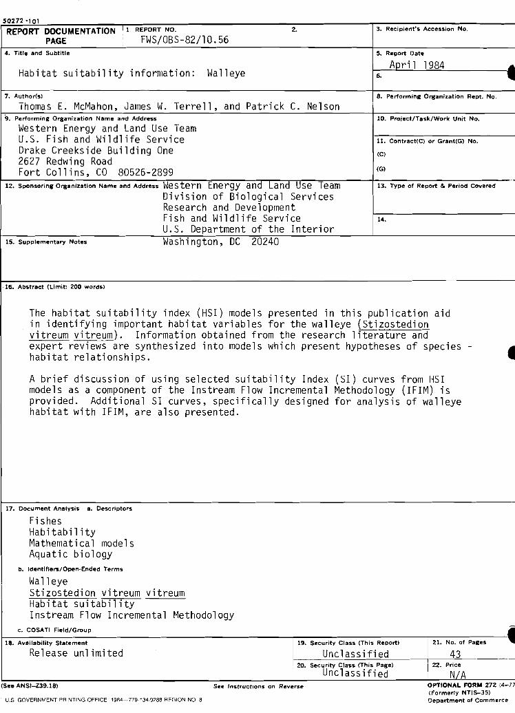
50272 101·REPORT DOCUMENTATION I 1. REPORT NO.

1

2•

3. Recipient's Accession No.

PAGE I FWSjOBS-82jlO.564. Title and Subtitle 5. Report Date

Anr t 1 1984 ...Habitat suitability information: Walleye 6. ..

7. Author(s) 8. Performing Organization Rept. No.

Thomas E. McMahon, James W. Terrell, and Patrick C. Nelson9. Performing Organization Name and Address 10. Project/Task/Work Unit No.

Western Energy and Land Use TeamU.S. Fish and Wildlife Service 11. Conlracl(C) or Grant(G) No.

Drake Creekside Building One (C)

2627 Redwing RoadFort Collins, CO 80526-2899 (G)

12. Sponsoring Organization Name and Address ~~este rn Energy and Land Use Team.'-

13. Type of Report & Period Covered

Division of Biological ServicesResearch and DevelopmentFish and Wildlife Service 14.

U.S. Department of the Interior15. Supplementary Notes Washington, DC 20240

1&. Abstract (Limit: 200 words)

The habitat suitability index (HSI) mode 1s presented in this publication aidin identifying important habitat variables for the walleye (Stizostedionvitreum vitreum). Information obtained from the research 1iterature andexpert reviews are synthesized into models which present hypotheses of species - -habitat relationships.

A brief discussion of using selected suitability Index (SI) curves from HSImodels as a component of the Instream Flow Incremental Methodology (IFIM) isprovided. Additional SI curves, specifically designed for analysis of walleyehabitat with IFIM, are also presented.

17. Document Analysis a. Desc ri ptors

FishesHabi tabil i tyMathematical modelsAquatic biology

b. Identifiers/Open.Ended Terms

WalleyeStizostedion vitreum vitreumHabitat suitabilityInstream Flow Incremental ~lethodology

c. COSATI Field/Group t18. Availabilily Stalement 19. Security Class (This Report) 21. No. of Pages

Release unlimited Unclassified 43I 20. Securily Class (This Page) 22. Price

i Unclassified N/A(See ANSI-Z39.18) See Instructions on Reverse

U.S GOVERNMENT PRINTING OFFICE: 1984~77g·1349288 REGION NO.8

OPTIONAL FORM 272 (4-77(Formerly NTI>35)Department of Commerce

CJ<VUO'" ISlandS

Habitat suitabi Iity inrmation :"c"ahon I Ihom E,

24962SU61 .U54 no, 82

~~'~1~1" ~l~ 11111111_111__1111111 _--..J

1-- -I II I......

'2 ""'"-­,•

,,,r- - - ------6:,-----

L-.__ ,I ---,

I : ,-- -I I

I

f 8104Q9lcaJDC

.ces

)( Estern Energv .nd Land Use TeamLpelown WV

* altonal Coaslal Ecosvstems TeamSlidell LA

REGION 1Regionltl DirectorU,S. Fish and Wildlife ServiceLloyd FiveHundred BUilding, Suile 1692500 N E. Multnomah StreetPortland, Oregon 971 n

REGION :2Regional DirectorU.S. Fish and Wildlife ServiceP,O. Box 1306Albuquerque, New Mexico 87103

REGION JRegional DirectorU.S. Fi h and Wildlife ServiceFederal Building. Fort SnellingTwin rilles, innesota 55111

REGION 4 REGION 5Regional DirectorU.s. Fish and Wildlife ServiceOne Gateway CenterNewton Comer, \1assachu5Clls 02158

REGION 6Regional DirectorU.S. Fish lindWildlife ServiceP.O. Box 25486Denver Federa CenterDenver, COlorado 80225

REGION 7Regional DirectorU.S. Fish and Wildlire Service1011 E. Tudor RoadAnchorage, Alaska 99503

DEPARTMENT OF THE INTERIORu.s. FISH AND WILDLIFE SERVICE

As the Nation's principal conservation agency, the Department of the Interior has respon­sibility for most of our .nationally owned public lands and natural resources. This includesfostering the wisest use of our land and water resources, protecting our fIsh and wildlife,preserving th&environmental and cultural values of our national parks and historical places,and providing for the enjoyment of life throulh outdoor recreation. The Department as·sesses our energy and mineral resources and works to assure that their development is inthe best interests of all our people. The Department also has a major responsibility forAmerican Indian reservation communities and for people who live in island territories underU.S. administration.