SK361. U54no . 82­10.41

v'·-'ry1\' :~ilal Wetlands Research Center( .J FIst and wtldUfe'7 CajundomeBoolevanll,,;J.yettc, La. 70506

FWS/OS5-8211 0.41SEPTEMBER 1983

HABITAT SUITABILITY INFORMATION:BLACKNOSE DACE

L...--~~._,,"",,:\ and Wildlife Service

. Department of the Interior

Thi s model is designed to be used by the Division of Ecological Servi~es

i n conjunction with the Habitat Evaluation Procedures.

FWS/OBS-82/10.41September 1983

HABITAT SUITABILITY INFORMATION: BLACKNOSE DACE

by

Joan G. Trialand

Jon G. StanleyMaine Cooperative Fishery Research Unit

University of MaineOrono, ME 04469

Mary BatchellerGlen Gebhart

andO. Eugene Maughan

Oklahoma Cooperative Fishery Research UnitOklahoma State University

Stillwater, OK 74074

Patrick C. NelsonInstream Flow and Aquatic Systems Group

Drake Creekside Building One2627 Redwing Road

Fort Collins, CO 80526

Project Officers

Robert F. RaleighJames W. Terrell

Habitat Evaluation Procedures GroupDrake Creekside Building One

2627 Redwing RoadFort Collins, CO 80526

Performed forWestern Energy and tand Use Team

Division of Biological ServicesResearch and DevelopmentFish and Wildlif~ Service

U.S. Department of the InteriorWashington, DC 20240

This report should be cited as:

Trial, J. G., J. G. Stanley, M. Batcheller, G. Gebhart, O. E. Maughan, andP. C. Nelson. 1983. Habitat suitability information: Blacknose dace.U.S. Dept. Int., Fish Wildl. Servo FWS/OBS-82/10.41. 28 pp.

PREFACE

The habitat use information and Habitat Suitability Index (HSI) modelspresented in this document are an aid for impact assessment and habitat manage­ment activities. Literature concerning a species' habitat requirements andpreferences is reviewed and then synthesized into subjective HSI models, whichare scaled to produce an index between 0 (unsuitable habitat) and 1 (optimalhabitat). Assumptions used to transform habitat use information into thesemathematical models are noted, and guidelines for model application aredescri bed. Any models found in the 1i terature whi ch may also be used tocalculate an HSI are cited, and simplified HSI models, based on what theauthors believe to be the most important habitat characteristics for thisspecies, are presented. Also included is a brief discussion of SuitabilityIndex (SI) curves as used in the Instream Flow Incremental Methodology.(IFIM) and a discussion of SI curves available for the IFIM analysis ofblacknose dace habitat.

Use of habitat information presented in this publication for impactassessment requires the setting of clear study objectives. Methods for reduc­ing model complexity and recommended measurement techniques for model variablesare presented in Terrell et al. (1982).1 A discussion of HSI model buildingtechniques, including the component approach, is presented in U.S. Fish andWildlife Service (1981).2

The HSI models presented herein are complex hypotheses of species-habitatrelationships, not statements of proven cause and effect relationships. Themodels have notl)een tested against field data. For this reason, the FWSencourages model users to convey comments and suggestions that may help usincrease the utility and effectiveness of this habitat-based approach to fishand wildlife planning. Please send comments to:

Habitat Evaluation Procedures GroupWestern Energy and Land Use TeamU.S. Fish and Wildlife Service2627 Redwing RoadFt. Collins, CO 80526

'Te rr-e l l , J. W., T. E. McMahon, P. D. Inskip, R. F. Raleigh, and K. L.Williamson (1982). Habitat sUitability index models: Appendix A. Guidelinesfor riverine and lacustrine applications of fish HSI models with the habitatevaluation procedures. U.S. Dept. Int., Fish Wildl. Servo FWS/OBS-82/l0.A.54 pp.

2U.S. Fish and Wildlife Service.habitat suitability index models.Serv., Div. Ecol. Servo n.p.

1981. Standards for the development of103 ESM. U.S. Dept. Int., Fish Wildl.

iii

CONTENTS

Page

PREFACE iiiACKNOWLEDGMENTS vi

HABITAT USE INFORMATION 1Genera 1 1Age, Growth, and Food 1Reproduct ion 1Specific Habitat Requirements 2

HABITAT SUITABILITY INDEX (HSI) MODELS................................. 3Model Applicability 3Model Description - Riverine...................................... 3Mode 1 Descri pt ion - Lacustri ne 5Suitability Index (SI) Graphs for Model Variables................. 6Riveri ne Model.................................................... 14Lacustri ne Model.................................................. 15Interpret i ng Model Outputs 16

ADDITIONAL HABITAT MODELS 16Mode 1 1 16Model 2 16

INSTREAM FLOW INCREMENTAL METHODOLOGY (IFIM) 22Suitability Index Graphs as Used in IFIM 22Avail abil ity of Graphs for Use in I FIM 24

REFERENCES 26

v

ACKNOWLEDGMENTS

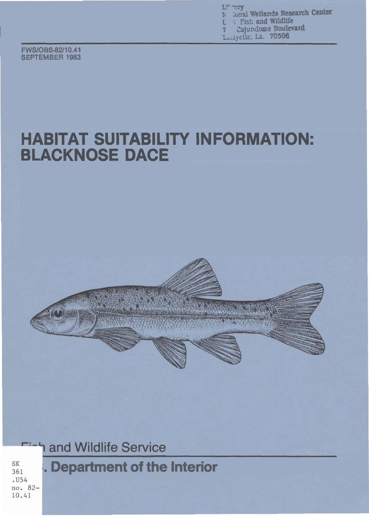
We thank V. G. Bartnick and J. G. Gee for their suggestions and commentson earlier manuscripts. Word processing was provided by C. Gulzow andD. Ibarra. Editorial review was by C. Short. K. Twomey assisted withfinalizing the manuscript. The cover illustration is from Freshwater Fishesof Canada 1973, Bulletin 184, Fisheries Research Board of Canada, by W. B.Scott and E. J. Crossman.

vi

BLACKNOSE DACE (Rhinichthys atratulus)

HABITAT USE INFORMATION

Genera 1

The blacknose dace (Rhinichthys atratulus) is distributed from Manitobato Nebraska, east to the Maritime Provinces, and south along both sides of theAppalachian Mountains to Georgia and Alabama (Lee et al. 1980). Three sub­species are recognized within this range: R. a. obtusus; R. a. atratulus; andR. ~. meleagris (Lee et al. 1980). Artificial hybrids of-br-acknose dace andlongnose dace (R. cataractae) can be produced in the laboratory but do notoccur in nature-because of behavioral isolating mechanisms (Bartnik 1970a;Howell and Villa 1976).

Age, Growth, and Food

Blacknose dace usually mature at age II (Schwartz 1958; Noble 1965;Bartnik 1970a; Bragg and Stasiak 1978), although, in Manitoba, spawning didnot occur until age III (Gibbons 1971). The blacknose dace is short-lived(Scott and Crossman 1973). Noble (1965) reported that few fish reach age III.Fry, 5 mm long at hatching (Traver 1929), grow quickly and are 29 mm long byage I and 45 mm long by age II (Noble 1965). The species seldom reaches102 mm (Trautman 1957).

Blacknose dace eat primarily aquatic invertebrates, such as chironomidsand other nymphs and larvae (Breder and Crawford 1922; Traver 1929; Churchilland Over 1938; Noble 1965; Tarter 1970; Gibbons and Gee 1972). The diet mayalso include terrestrial insects (Tarter 1970) and plants (Breder and Crawford1922; Flemer and Woolcott 1966). Foraging by fry occurs on invertebrates inquiet, shallow water with soft, silty substrates (Tarter 1970). As the fishgrow, they forage on invertebrates associated with riffles and deep eddyingpools (Tarter 1970).

Reproduction

Blacknose dace breed in May, June, and July (Raney 1940; Schwartz 1958;Noble 1965; Bartnik 1970a), at temperatures ranging from 15.6 (Schwartz 1958)to 22° C (Traver 1929). Spawning in the northern part of the range beginswhen the water temperature reaches 21° C (Raney 1940; Scott and Crossman1973). Blacknose dace spawn in shallow water of streams (Traver 1929). Waterdepths of less than 25 cm (Schwartz 1958), velocities of 20 to 45 cm/sec

1

(Bartnik 1970b), and uniform gravel substrates (Raney 1940; Bartnik 1970a;Bragg and Stasiak 1978) are preferred. The most common spawning sites areriffles, although spawning may occur in pools (Traver 1929; Raney 1940;Schwartz 1958; Bartnik 1970a; Bragg and Stasiak 1978).

Conflicting descriptions of blacknose dace spawning behavior reflect thedifference between subspecies (Raney 1940; Scott and Crossman 1973). MaleB. ~. meleagris establish and defend territories (Churchill and Over 1938;Harlan and Speaker 1951; Bartnik 1970a). Territorial males spawn singly witha sequence of several females. In contrast, males of R. a. atratulus (Traver1929) and R. a. obtusus (Schwartz 1958) are not territorial. Nonterritorialmales mate- in- mass with one female (Raney 1940). Vigorous movements duringspawning cause a depression in the substrate, producing a poorly constructednest (Raney 1940; Schwartz 1958; Bartnik 1970a; Bragg and Stasiak 1978).Females lay from 428 to 1,116 eggs, averaging 746 (Traver 1929). Fecundityincreases with body length of the female (Noble 1965).

Specific Habitat Requirements

Adult. Blacknose dace typically are found in the pools of small streams(Traver 1929; Fish 1932) but may be found in other habitats (Whitworth et al.1968). The species is collected occasionally in large rivers (Trautman 1957)and rarely in lakes (Fish 1932; Scarola 1973) and river impoundments (Harlanand Speaker 1951). Blacknose dace occupy clear streams (Trautman 1957;Armstrong and Williams 1971; Scott and Crossman 1973; Bragg and Stasiak 1978).Undercut banks. roots, brush, overhanging vegetation, and shaded areas areutilized as cover (Trautman 1957). Adult blacknose dace typically occur inrocky and gravelly streams (Harlan and Speaker 1951; Scarola 1973; Bragg andStasiak 1978) with highest densities over gravel-cobble substrates (Gibbonsand Gee 1972).

The blacknose dace prefers swift streams (Traver 1929; Harlan and Speaker1951; Scarola 1973). Greatest densities of blacknose dace adults occur whensurface water velocities are between 15 and 45 em/sec (Gibbons and Gee 1972).The species is common at gradients of 11.4 and 23.3 m/km, but almost entirelyabsent at 67.2 m/km (Burton and Odum 1945). Low gradients « 5 m/km) are alsoavoided (Trautman 1957; Gibbons and Gee 1972). The upper incipient lethaltemperature for blacknose dace is 29.3° C (Hart 1952).

Blacknose dace migrate from cool headwater streams into rivers to over­wi nter (Noble 1965). Traver (1929) observed speci men sin deep water duri ngwinter.

Embryo. The spawning sites preferred by the adults are assumed optimalfor embryo survival. Blacknose dace eggs incubate in slow (Raney 1940; Bartnik1970a) to fast (Scott and Crossman 1973) currents. varying from 7 to 60 em/sec,but the majority are found at velocities between 20 and 45 em/sec (Bartnik1970b). Spawni ng occurs in water depths from several centimeters (Traver1929) to 30.5 cm (Scott and Crossman 1973), the preferred depth being 25 em(Schwartz 1958). Blacknose dace spawn on substrates of sand (Raney 1940),gravel (Traver 1929; Fish 1932; Raney 1940; Bragg and Stasiak 1978), and

2

cobble (Harlan and Speaker 1951). Bartnik (l970a) found nests o.ccurring insubstrates with particles 2.5 cm or smaller. Water temperature ranges from 15to 22° C during embryo incubation (Traver 1929; Schwartz 1958).

Fry. High densities of fry of the blacknose dace are observed over siltand sand substrates where the water velocity is less than 15 cm/sec (Gibbonsand Gee 1972). Fry largely occupy shoals and pool margins (Traver 1929;Minckley 1963).

Juvenile. Juvenile blacknose dace- occur over substrates of sand, reachh~ghest densities over gravel, and frequent areas with small rocks and boulders(Witt 1970; Gibbons and Gee 1972). High numbers are associated with surfacevelocities from 15 to 30 cm/sec (Gibbons and Gee 1972).

HABITAT SUITABILITY INDEX (HSI) MODELS

Model Applicability

Geographic area. The model applies throughout the range of the blacknosedace in North America.

Season. The model assesses the ability of a habitat to support self­sustaining populations of blacknose dace throughout the year.

Cover types. The model applies to freshwater streams, rivers, and lakes.

Minimum habitat area. The minimum area of contiguous suitable habitatfor sustaining a population of blacknose dace has not been established.

Verification level. The blacknose dace model produces an index between 0and 1 that we believe has a positive relationship to habitat carrying capacity.Model output has not been compared to production or standing crop estimates,but field testing is planned. HSI's calculated from sample data sets appearedto be reasonable. These sample data sets are discussed in greater detailfollowing the presentation of the model.

Model Description - Riverine

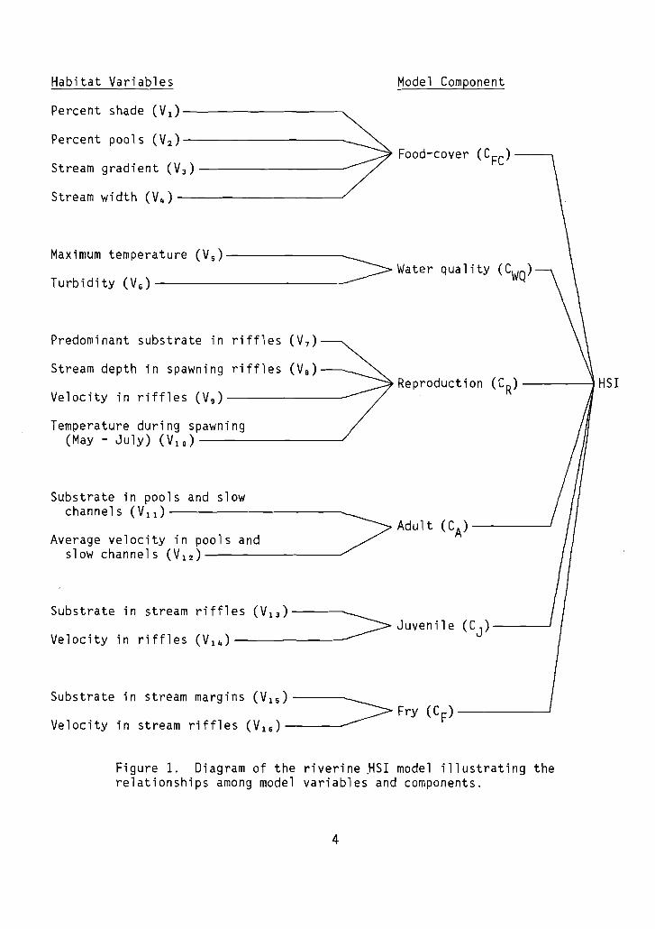
The riverine model (Fig. 1) consists of six components: food-cover(CF-C); water quality (CWQ); reproduction (CR); adult (CA); juvenile (CJ ) ; and

fry (CF).

The model uses a modified limiting factor approach. Model variables withvalues between 0.4 and 1.0 are used to compute component values. If componentvalues, in tarn, are between 0.4 and 1.0, they are used to compute the HSIvalue. However, any value less than 0.4 for variables or components is assumedto be limiting and, thus, overrides computed model values.

3

Habitat Variables Model Component

Substrate in stream margins (V lS)----~~_ _ _ __~ Fry (C F)Velocity in stream riffles (V l 6) .

Substrate in stream riffles (Vl3)--~>___________~ Juvenile (CJ)Velocity in riffles (V l 4) .

Reproduct ion (C R) -------; HSI

Food-cover (C FC)-----,

Percent shade (Vl)------------------~

Percent pools (V2)--------------------~

Stream gradient (V3)------------------~

Stream width (V4) -------------------J

Predominant substrate in riffles (V 7 )

Stream depth in spawning riffles (Va)

Velocity in riffles (V9)--------------~

Maximum temperature (Vs)------------~

> Water qual ity (CWQ)Turbidity (V6)----------------------~

Temperature during spawning(May - J u1y) (V10 ) -----------/

Substrate in pools and slowchannels (Vl l) --------------------~

__ _ _ _ _ _ ~~ Adult (CA)Average velocity in pools and ~

slow channels (V l 2)

Figure 1. Diagram of the riverine ~SI model illustrating therelationships among model variables and components.

4

Food-cover component. The area of shaded streambed expressed as apercentage of total streambed, is an estimate of instream cover (VI)' Percent

pools (V 2 ), stream gradient (V 3 ) , and stream width (V 4 ) are related to the

amount and quality of cover available in a stream for all life stages ofblacknose dace. Pool-riffle ratio also is an indirect measure of aquaticinsect production.

Water quality component. Maximum temperature (V s) is included because it

affects growth, distribution, survival, and behavior. Turbidity (V s ) affects

the distribution of blacknose dace.

Reproduction component. Spawning requirements are defined by the rifflesubstrate (V 7 ) , stream depth in spawning riffles (Va), and velocity in riffles

(V g ) . Water temperature (V lD ) affects spawning and embryo development and

survival.

Adult component. Adult habitat is defined by substrate (VII) and velocity

(V 12 ) in pools and slow channels, the two most important environmental vari­

ables. The model takes into account habitat partitioning between age groups.

J uvenile com p0 nent . Subst rate ( V1 3) and vel 0 city ( V1 4 ) i n riff1es are

adequate to describe juvenile habitat.

Fry component. Suitable habitat of fry can be defined by substrate (VIS)

and velocity (VIS) in stream margins.

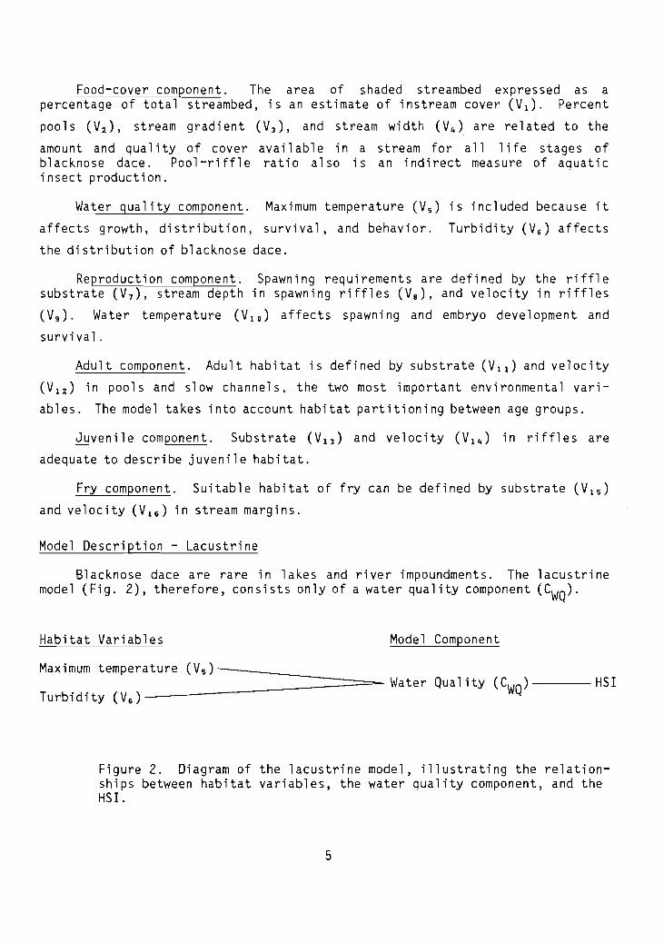
Model Description - Lacustrine

Blacknose dace are rare in lakes and river impoundments. The lacustrinemodel (Fig. 2), therefore, consists only of a water quality component (CWQ)'

Habitat Variables Model Component

Maximum tempera~t,~u~r~e~(~v~s~)~--====================-_ Water Quality (CWQ)---HSI

Figure 2. Diagram of the lacustrine model, illustrating the relation­ships between habitat variables, the water quality component, and theHSI.

5

Water quality component. Maximum temperature (V s ) and turbidity (V 6 ) areincluded in this component because they are important 1 imiting factors.

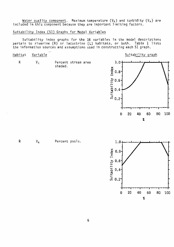
Suitability Index (51) Graphs for Model Variables

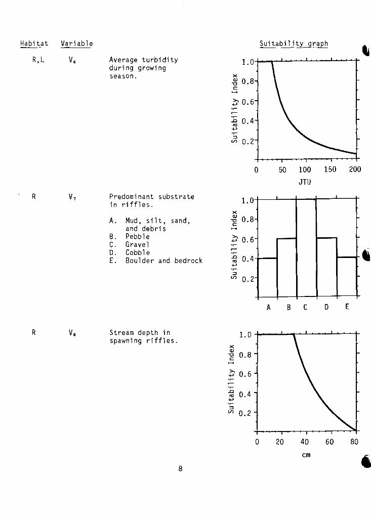
Suitability index graphs for the 16 variables in the model descriptionsperta into ri veri ne (R) or 1acustri ne (L) habitats, or both. Table 1 1i ststhe information sources and assumptions used in constructing each 51 graph.

Habitat Variable

R Percent stream areashaded.

Suitability graph

xcu-g 0.8.....

~0.6.,....,...~ 0.4~

::3

V) 0.2

o 20 40 60 80 100

%

R Percent pools. 1.0

x0.8cu

"'Ct:.....~ 0.6

.,...0.4.D

10~.,...::3 0.2V)

6

o 20 40 60 80 100

%

Habitat Variable Suitability graph

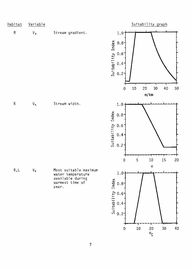
R V3 StreaR1 gradient. 1.0

x 0.8Q)-0s::......>, 0.6~.,.....,.... 0.4..c~~

::::l 0.2U')

0 10 20 30 40 50

m/km

R V4 Stream width. 1.0

xQ) 0.8-0s::......>, 0.6~.,....

..c 0.4~~.,....::::l 0.2U')

R,L Most suitable maximumwater temperatureavailable duringwarmest time ofyear.

0 5 10 15 20

m

1.0xQ)

0.8-0s::......

~ 0.6.,....

..c 0.4~

~

::::lU') 0.2

7

Habitat Variable

Average turbidityduring growingseason.

1.0

xQ) 0.8"'Cc:.....~ 0.6.,...

''''' 0.4.010+>.,...:::::l

0.2(/)

Suitability graph

o 50 100

JTU

150 200

R V7 Predominant substrate 1.0in riffles.x

A. Mud, silt, sand,Q) 0.8"'Cc:

and debris .....B. Pebble ~ 0.6C. Gravel .,...

D. Cobble .,...

E. Boulder and bedrock .0 0.410....,.,...

:::::l(/) 0.2

-

...

R Stream depth inspawning riffles.

8

1.0xQ)

0.8"'Cc:.....

~ 0.6.,...r-.,....0 0.410....,.,...

:::::l(/) 0.2

o

A

20

B C

40

em

o

60

E

,80

Habitat Variable

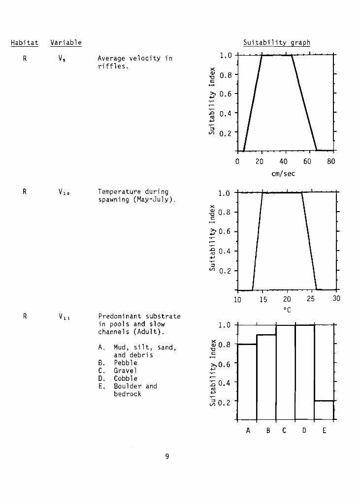
Average velocity inriffles.

1.0

xQ) 0.8"0c......

.;, 0.6......r-......oD 0.410...........;:,Vl 0.2

Suitability graph

0 20 40 60 80

em/sec

R VlO Temperature during 1.0 I

spawning (May-July). \x~ 0.8 -c \......

';'0.6-......r-......~ 0.4 -+-'......;:,

Vl 0.2 -

\10 15 20 25 30

°CR V11 Predominant substrate

in pools and slow 1.0channels (Adult).

xA. Mud, silt, sand, Q) 0.8

"0

and debris c......B. Pebble ~0.6C. Gravel ...........D. Cobble r-

E. Boulder and :0 0.410

bedrock ...........a0.2

r-

9

A B C o E

Habitat

R

Variable

Average velocity inpools and slowchannels (Adult).

1.0

x(])

-g 0.8

1)0.6

~ 0.4.j...)

'r-::::l

V1 0.2

Suitability graph

o 20 40

ern/sec60 80

R V13 Predominant substrate 1.0in stream riffles(Juvenile).

~ 0.8A. Mud, si It, sand, e

1-1

and debris c-, 0.6B. Pebble ....

'r-

C. Gravel:0 0.4D. Cobble to

E. Boulder and ....'r-

bedrock ~ 0.2

I

-

-

R Velocity in riffles(Juvenile).

10

x~ 0.8e

1-1

1) 0.6

:0 0.4to~

'r-

~ 0.2

a

A B

20

C

40

em/sec

o

60

E

80

Habitat Variable

R Predominant substratealong.stream margins(Fry) .

A. Mud, silt, sand,and debris

B. PebbleC. GravelD. CobbleE. Boulder and

bedrock

X

Q.J a 0"'0 • uC

>,....., 0.6

'r-

-g 0.4.....,

;:;Vl 0.2

Suitability graphI

R Velocity alongstream margins(Fry) .

11

XQ.J

~ 0.8

~ 0.6'r-

.D2 0.4;:;

Vl 0.2

o

A

20

B c

40

cm/sec

o

60

E

80

Table 1. Data sources and assumptions for blacknose dacesuitability indices.

V7

Variable and source

Trautman 1957Noble 1965

Traver 1929Schwartz 1958Noble 1965Whitworth et al. 1968Tarter 1970Scott and Crossman 1973

Burton and Odum 1945Gibbons and Gee 1972

Fish 1932Starrett 1950Trautman 1957Scarola 1973Bragg and Stasiak 1978

Hart 1952Minckley 1963Noble 1965Terpin et al. 1976

Trautman 1957Armstrong and Williams 1971

Traver 1929Fish 1932Raney 1940Harlan and Speaker 1951Bartnik 1970aBragg and Stasiak 1978

Assumption

Since blacknose dace concentrate inareas with overhead cover and areseldom found where there is no canopyclosure, the majority of the streammust have overhead cover. Percent ofstream area shaded is an estimate ofpercent overhead cover.

Blacknose dace require both pools andriffles; 50 to 80% pools provideoptimum habitat for all life stages,reproduction, and food.

The gradients of streams where blacknosedace were abundant are optimal.

Widths of streams where populations werelarge are optimal.

Maximum summer temperatures in streamswhere blacknose dace were abundant areoptimal. Temperatures between upperincipient lethal and optimal levels aresut t ab1e.

Clear streams, where blacknose dace wereabundant, are optimal. Clear streamshave average turbidity less than 30 JTU.

Substrates where most nests were builtare optimal.

12

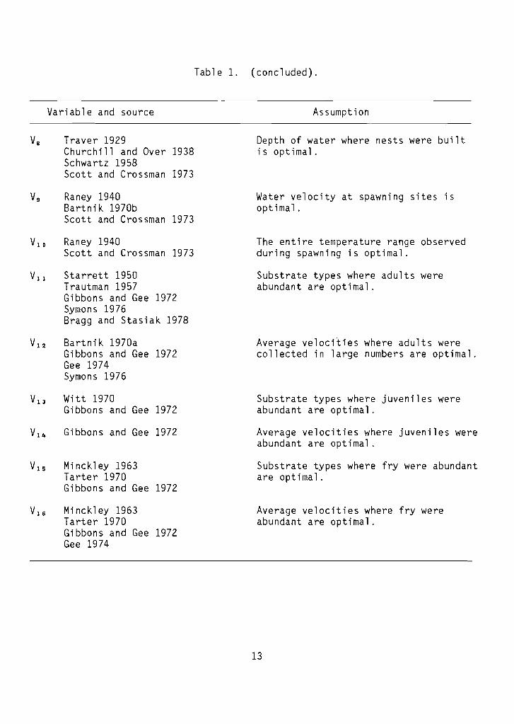
Table 1. (concluded).

Variable and source Assumption

Traver 1929Churchill and Over 1938Schwartz 1958Scott and Crossman 1973

Raney 1940Bartnik 1970bScott and Crossman 1973

Raney 1940Scott and Crossman 1973

Starrett 1950Trautman 1957Gibbons and Gee 1972Symons 1976Bragg and Stasiak 1978

Bartnik 1970aGibbons and Gee 1972Gee 1974Symons 1976

Witt 1970Gibbons and Gee 1972

Gibbons and Gee 1972

Minckley 1963Tarter 1970Gibbons and Gee 1972

Minckley 1963Tarter 1970Gibbons and Gee 1972Gee 1974

Depth of water where nests were builtis opt i ma 1.

Water velocity at spawning sites isoptimal.

The entire temperature range observedduring spawning is optimal.

Substrate types where adults wereabundant are optimal.

Average velocities where adults werecollected in large numbers are optimal.

Substrate types where juveniles wereabundant are optimal.

Average velocities where juveniles wereabundant are optimal.

Substrate types where fry were abundantare optimal.

Average velocities where fry wereabundant are optimal.

13

Riverine Model

Food-Cover eCF-C)'

CF =-c

Or, if any value ~ 0.4, CF-C = V1 , V2 , V3 , or V4 , whichever is lowest.

Water Quality (CWQ)'

CWQ

= (V s2 x V6)1/3

Or, if any value ~ 0.4, CWQ = Vs or V6 , whichever is lowest.

Reproduction eCR)'

C ­R -

1/4eV 7 x Va X Vg

2) + V1 0

2

Or, if any value ~ 0.4, CR = V7 , Va, Vg , or V1 0 , whichever is lowest.

This is an optional component.

CA

= (V 1 1 x V1 2)1/2

Or, if any value ~ 0.4, CA = V1 1 or V1 2 , whichever is lowest.

14

Juvenile (CJ).

This is an optional component.

1/2CJ = (V1 3 x V1 4 )

Or, if any value $ 0.4, CA = V1 3 or V1 4 , whichever is lowest.

This is an optional component.

1/2CF = (VIS x VIS)

Or, if any value $ 0.4, CA= VIS or VIS' whichever is lowest.

HSI determination.

. 1/3 linSpecles HSI = (CF-C x CWQ x CR) x (CA x CJ x CF)

Or, if any component $ 0.4, the HSI = CF-C' CWQ' CR' CA' CJ' or CF'whichever is lowest.

CA' CJ , and CF are optional; n = number of components in parenthesis.

Life stage HSI = CF-C x CWQ x Cappropriate life stage

Lacustrine Model

Water Quality.

CWQ

= (VS2 x V

6)1/3

Or, if any value $ 0.4, CWQ = Vs or Vs , whichever is lowest.

HSI determination.

HSI = CWQ

15

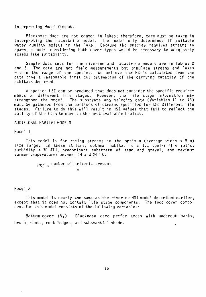
Interpreting Model Outputs

Blacknose dace are not common in lakes; therefore, care must be taken ininterpreting the lacustrine model. The model only determines if suitablewater quality exists in the lake. Because the species requires streams tospawn, a model considering both cover types would be necessary to adequatelyassess lake sUitability.

Sample data sets for the riverine and lacustrine models are in Tables 2and 3. The data are not field measurements but simulate streams and lakeswithin the range of the species. We believe the HSI's calculated from thedata give a reasonable first cut estimation of the carrying capacity of thehabitats depicted.

A species HSI can be produced that does not consider the specific require­ments of different life stages. However, the life stage information maystrengthen the model. The substrate and velocity data (Variables 11 to 16)must be gathered from the portions of streams specified for the different lifestages. Failure to do this will result in HSI values that fail to reflect theability of the fish to move to the best available habitat.

ADDITIONAL HABITAT MODELS

Mode 1 1

This model is for rating streams in the optimum (average width < 8 m)size range. In these streams, optimum habitat is a 1:1 pool-riffle ratio,turbidity < 30 JTU, predominant substrate of sand and gravel, and maximumsummer temperatures between 14 and 24° C.

HSI = number of criteria present4

Model 2

This model is nearly the same as the riverine HSI model described earlier,except that it does not contain life stage components. The food-cover compo­nent for this model consists of the following variables:

Bottom cover (V 1 ) . Blacknose dace prefer areas with undercut banks,

brush, roots, rock ledges, and substantial shade.

16

Table 2. Sample data sets using riverine HS1 model.

Data set 1 Data set 2 Data set 3Variable Data S1 Data S1 Data S1

% stream shaded Vi 50 1.0 30 0.6 10 0.4

% pools Vz 50 1.0 40 1.0 70 1.0

Gradient (m/km) V3 10 1.0 25 1.0 5 0.3

Width (m) V" 4 1.0 10 0.6 14 0.2

Max. temperature(0C) Vs 15 1.0 20 1.0 26 0.4

Turbi dity (JTU) VG 30 1.0 30 1.0 80 0.3

Dominant substrateclass in riffles V7 C 1.0 B 0.6 B 0.6

Depth (em) Ve 28 1.0 30 1.0 40 0.6

Velocity (em/sec) V9 40 1.0 35 1.0 20 1.0

Temperature (OC) VlO 20 1.0 20 1.0 23.5 0.9

Dominant substrateclass in pools(Adult) Vll C 1.0 A 0.8 A 0.8

Velocity (em/sec)(Adult) ViZ 13 1.0 11 1.0 3 1.0

Substrate classin riffl es(Juvenile) V13 C 1.0 B 1.0 B 1.0

Velocity (em/sec)(Juvenile) Vi" 35 1.0 36 1.0 15 1.0

Substrate classalong margins( Fry) ViS A 1.0 A 1.0 A 1.0

Velocity (em/sec)( Fry) V16 3 1.0 a 1.0 a 1.0

17

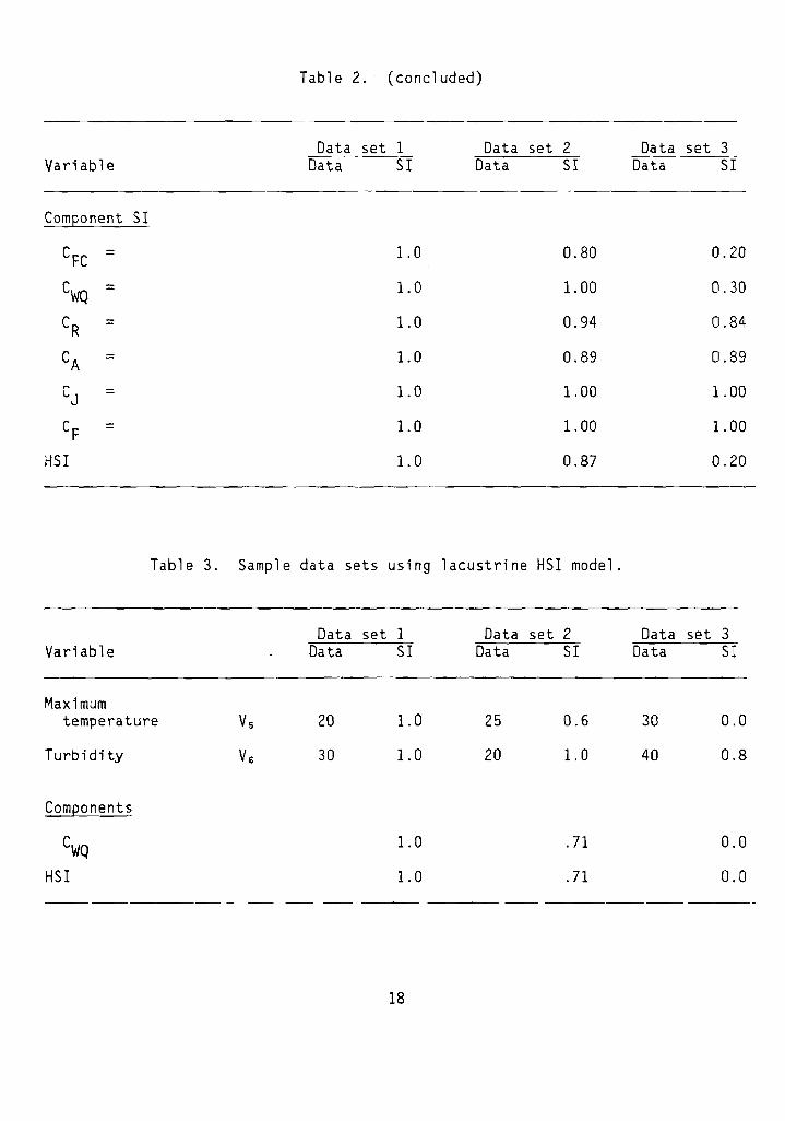
Table 2. (concluded)

Data set 1 Data set 2 Data set 3Variable Data SI Data SI Data SI

Component SI

CFC = 1.0 0.80 0.20

CWQ = 1.0 1. 00 0.30

CR = 1.0 0.94 0.84

CA = 1.0 0.89 0.89

CJ = 1.0 1. 00 1.00

CF = 1.0 1.00 1.00

HSI 1.0 0.87 0.20

Table 3. Sample data sets using lacustrine HSI model.

Data set 1 Data set 2 Data set 3Variable Data SI Data SI Data SI

Maximumtemperature Vs 20 1.0 25 0.6 30 0.0

Turbidity Vr, 30 1.0 20 1.0 40 0.8

Components

CWQ 1.0 .71 0.0

HSI 1.0 .71 0.0

18

Estimated percent of bottom shaded by a vertical projection of,overhangingvegetation, undercut banks, brush, roots, and rock ledges:

Rat i ng

a) > 50%

b) 25-50%

c) < 25%

0,8-1. 0

0.6-0.7

0.4-9.5

Percent~ (V 2 ) . Blacknose dace require both pools and riffles.

Spawning occurs in both pools and riffles, and the species overwinters inpools. Percent pools during normal flow:

Rating

a) 15-75%

b) 10-14% or 76-85%

c) < 10% or > 85%

0.8-1. 0

0.6-0.7

0.4-0.5

Stream gradi ent (V 3 ) . Bl acknose dace prefer moderate to hi gh gradi ent

streams. Stream gradi ent:

Rating

a) 8-25 m/km

b) 6-7m/km or 26-37 m/km

c) < 6 or > 37 m/km

0.8-1. 0

0.3-0.7

0.1-0.2

Width (V4 ) . Small streams are preferred. Stream width at normal flows:

Rating

a) < 8 m

b) 8-12 m

c) > 12 m

0.8-1. 0

0.4-0.7

0.2-0.3

The water quality component (CWQ) for Model 2 consists of the following

variables:

19

Maximum temperature (V s ) . High blacknose dace densities are associated

with low water temperatures. The species' upper incipient lethal temperatureis 29.3° C. Maximum summer temperature:

Rating

a)

b)

c)

13-15° C or 25-27° C

< 13 or > 27° C

0.8-1. 0

0.3-0.7

0.0-0.2

Turbidity (V s ) . Blacknose dace prefer clear streams. Turbidity at

norma 1 f1 ows :

Rating

a)

b)

c)

< 50 JTU

50-90 JTU

> 90 JTU

0.8-1. 0

0.4-0.7

0.0-0.3

The reproduction component (C R) for Model 2 consists of the following

variables:

Substrate (V 7 ) . Areas with substrate particles < 2.5 cm are preferred as

spawning sites. Substrate in moderate current areas:

Rating

a) Silt, sand, pebble, orgravel (particle diameter~ 5.0 cm)

b) Cobble or boulder(> 5.0 cm)

c) Bedrock or rootedvegetation

20

0.8-1.0

0.2-0.6

0.1

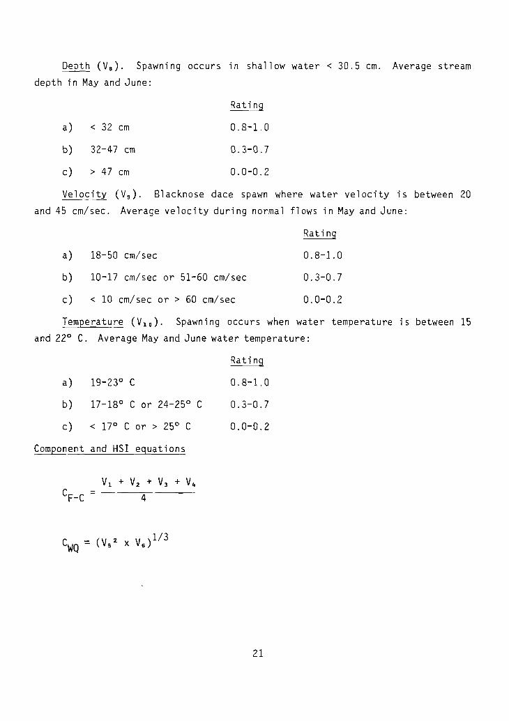
Depth (VB)' Spawning occurs in shallow water < 30.5 em. Average stream

depth in May and June:

a) < 32 em

b) 32-47 em

c) > 47 em

0.8-1.0

0.3-0.7

0.0-0.2

Velocity (V g ) . Blaeknose dace spawn where water velocity is between 20

and 45 em/sec. Average velocity during normal flows in May and June:

Rating

a) 18-50 em/sec

b) 10-17 em/sec or 51-60 em/sec

c) < 10 em/sec or > 60 em/sec

0.8-1.0

0.3-0.7

0.0-0.2

Temperature (V 1 0 ) ' Spawning occurs when water temperature is between 15

and 22° C. Average May and June water temperature:

Rating

a) 19-23° C

b) 17-18° C or 24-25° C

c) < 17° C or > 25° C

Component and HSI equations

VI + V2 + V3 + V4

CF-C = 4

0.8-1. 0

0.3-0.7

0.0-0.2

21

C =R

1/4(V7 X Va X V2) + V1 D

2

1/3HSI = (CF-C X CWO X CR)

Or, if any component value ~ 0.4, the HSI = CF-C' CWO' or CR' whichever is thelowest.

INSTREAM FLOW INCREMENTAL METHODOLOGY

The U.S. Fish and Wildlife Service's Instream Flow Incremental Methodology(IFIM), as outlined by Bovee 1982, is a set of ideas used to assess instreamflow problems. The Physical Habitat Simulation System (PHABSIM), described byMilhous et al. 1981, is one component of IFIM that can be used by investigatorsinterested in determining the amount of available instream habitat for a fishspecies as a function of streamflow. The output generated by PHABS1M can beused for several IFIM habitat display and interpretation techniques, including:

1. Optimization. Determination of monthly flows that minimize habitatreductions for species and life stages of interest;

2. Habitat Time Series. Determination of the impact of a project onhabitat by imposing project operation curves over historical flowrecords and integrating the difference between the curves; and

3. Effective Habitat Time Series. Calculation of the habitat require­ments of each life stage of a fish species at a given time by usinghabitat ratios (relative spatial requirements of various lifestages).

Suitability Index Graphs as Used in IFIM

PHABSIM utilizes Suitability Index graphs (SI curves) that describe theinstream suitability of the habitat variables most closely related to streamhydraulics and channel structure (velocity, depth, substrate, temperature, andcover) for each major life stage of a given fish species (spawning, egg incuba­tion, fry, juvenile, and adult). The specific curves required for a PHABS1Manalysis represent the hydraulic-related parameters for which a species orlife stage demonstrates a strong preference (i .e., a pelagic species that onlyshows preferences for velocity and temperature will have very broad curves fordepth, substrate, and cover). Instream Flow Information Papers 11 (Milhouset al. 1981) and 12 (Bovee 1982) should be reviewed carefully before using anycurves for a PHABSIM analysis. SI curves used with the 1F1M that are generatedfrom empirical microhabitat data are quite similar in appearance to the moregenera 1i zed 1i terature-based SI curves deve loped in many HSI models (Armouret al. 1983). These two types of SI curves are interchangeable, in some

22

cases, after conversion to the same units of measurement (English~ metric, orcodes). 51 curve validity is dependent on the quality and quantity of informa­tion used to generate the curve. The curves used need to accurately reflectthe conditions and assumptions inherent to the model(s) used to aggregate thecurve-generated 51 values into a measure of habd t at suitability. If thenecessary curves are unavailable or if available curves are inadequate (i.e.,built on different assumptions), a new set of curves should be generated (datacollection and analyses techniques for curve generation will be included in aforthcoming Instream Flow Information Paper).

There are several ways to develop 51 curves. The method selected dependson the habitat model that will be used and the ava il ab1e database for thespecies. The validity of the curve is not obvious and, therefore, the methodby whi ch the curve is generated and the quality of the database are veryimportant. Care al so must be taken to choose the habitat model most appro­priate for the specific study or evaluation; the choice of models will deter­mine the type of 51 curves that will be used. For example, in an H5I model,an 51 curve for velocity usually reflects suitability of average channel(stream) velocity (i.e., a macrohabitat descriptor); in an IFIM analysis, 51curves for velocity are assumed to represent suitability of the velocity atthe point in the stream occupied by a fish (i .e., a microhabitat descriptor)(Armour et a1. 1983).

A system with standard terminology has been developed for classifying 51curve sets and describing the database used to construct the curves in IFIMapplications. The classification is not intended to define the quality of thedata or the accuracy of the curves. There are four categories in the classi­fication. A literature-based curve (category one) has a generalized descrip­tion or summary of habitat preferences from the 1iterature as its database.This type of curve usually is based on information in published references onthe upper and lower limits of a variable for a species (e.g., juveniles areusually found at water depths of 0.3-1.0 m). Occasionally, the reference alsocontains information on the optimal or preferred condition within the limitsof tolerance (e.g., juveniles are found at water depths of 0.3-1.0 m, but aremost common at depths from 0.4-0.6 m). Most of the 51 curves presently avail­able for use with the IFIM, and virtually all of the 51 curves published inthe H5I series for depth, velocity, and substrate, are first generation curves.

Utilization curves (category two) are based on a frequency analysis offish observations in the stream environment with the habitat variables measuredat each sighting [see Instream Flow Information Paper 3 (Bovee and Cochnauer1977) and Instream Flow Information Paper 12 (Bovee 1982:173-196)]. Thesecurves are designated as utilization curves because they depict the habitatconditions a fish will use within a specific range of available conditions.Because of the way the data are collected for utilization curves, the resultingfunction represents the probability of occurrence of a particular environmentalcondition, given the presence of a fish of a particular species, P(EIF).Utilization curves are generally more precise for IFIM applications than1iterature-based curves because they are based on specific measurements ofhabitat characteristics where the fish actually occur. However, utilizationcurves may not be transferable to streams that differ substantially in sizeand complexity from the streams where the data were obtained.

23

A preference curve (category three) is a utilization curve that has beencorrected for environmental bias. For example, if 50% of the fish are foundin pools over 1.0 m deep, but only 10% of the stream has such pools, the fishare actively selecting that type of habitat. Preference curves approximatethe function of the probabil i ty of occurrence of a fi sh, given a set ofenvironmental conditions:

P(F/E) ~P(EIF)peE)

Only a limited number of experimental data sets have been compiled into IFIMpreference curves. The development of these curves should be the goal of allnew curve development efforts.

The fourth category of curves are still largely conceptual. One typeunder consideration is a cover-conditioned, or season-conditioned, preferencecurve set. Such a curve set would consist of different depth-velocity prefer­ence curves as a function or condition of the type of cover present or thetime of year. No fourth category curves have been developed at this time.

The advantage of category three and four curves is the s i gni fi cantimprovement in precision and confidence in the curves when applied to streamssimilar to the streams where the original data were obtained. The degree ofincreased accuracy and transferability obtainable when applying these curvesto dissimilar streams is unknown. In theory, the curves should be widelytransferable to any stream in which the range of environmental conditions iswithin the range of conditions found in the streams from which the curves weredeveloped.

Availability of Graphs for Use in IFIM

No curves have been developed by the Instream Flow Group for the blacknosedace. HSI model information and curves may be used for IFIM analyses(Table 4). An investigator should consider the information carefully todetermine applicability in his area. No curves are available to describedepth preferences of adults, juveniles, or,fry.

24

Table 4. Availability of curves for IFIM analysis of blacknose dace habitat.

N(J"I

Spawning

Egg incubat ton

Fry

Juvenile

Adult

Velocitya

Use SI curve forVg •

Use SI curve for».;

Use SI curve forV16'

Use SI curve forVlifO

Use SI curve forV12'

Deptha

Use SI curve forVa-

Use SI curve forVs ·

No curve avail­able.

No curve avail­able.

No curve avail­able.

SUbstrateb,c Temperaturea Covera

Use SIb = 1.0 for Use SI curve for No curvesand, gravel, VI o- available.cobble (see text,pages 4 and 5).

Use SI = 1.0 for Use SI curve for No curvesand, gravel, V1 0 • available.cobble (see text,pages 4 and 5).

Use SI = 1.0 for Use SI curve for Use SI curvesilt and sand V5' for Vl'(see text, page 5).

Use SI = 1.0 for Use SI curve No SI curvesand, gravel, for V5' for Vi-cobble, boulder(see text, page 5).

Use SI = 1.0 for Use SI curve Use SI curvegravel and cobble for V5' for Vi-(see text, page 4).

aWhen use of SI curves is prescribed, refer to the appropriate curve in the HSI model section.

bUse SI = 1.0 if the habitat variable is optimal; but if the habitat variable is less than optimal, the usermust determine, by judgement, what is the most appropriate SI value.

cThe following categories may be used for IFIM analyses (see Bovee 1982):

1 = plant detritus/organic material2 = mud/soft clay3 = silt (particle size < 0.062 mm)4 = sand (particle size 0.062-2.000 mm)5 = gravel (particle size 2.0-64.0 mm)6 = cobble/rubble (particle size 64.0-250.0 mm)7 = boulder (particle size 250.0-4000.0 mm)8 = bedrock (solid rock)

REFERENCES

Armour, C. L., R. J. Fisher, and J. W. Terrell. 1983. Comparison andrecommendations for use of Habitat Evaluation Procedures (HEP) and theInstream Flow Incremental Methodology (IFIM) for aquatic analyses.Unpublished draft report. U.S. Dept. Int., Fish Wildl. Serv., WesternEnergy and Land Use Team, Fort Collins, CO. 42 pp.

Armstrong, J. G., and J. D. Williams. 1971. Cave and spring fishes of thesouthern bend of the Tennessee River. J. Tenn. Acad. Sci. 46:107-115.

Bartnik, V. G. 1970a. Reproductive isolation between two sympatric dace,Rhinichthys atratulus and R. cataractae, in Manitoba. J. Fish. Res.Board Can. 27: 2125-2141. -

Bartnik, V. G. 1970b. Reproductiveof dace, Rhinichthys cataractaeand Valley Rivers, Manitoba.84 pp. (Cited by Gee 1970).

isolation between two sympatric speciesand Rhi c i c hthysatratu1us, i nthe Min kM.S. Thesis, Univ. Manitoba, Winnipeg.

Bovee, K. D. 1982. A qui de to stream habitat analysis using the InstreamFlow Incremental Methodology. Instream Flow Information Paper 12. U.S.Dept. Int., Fish Wildl. Servo FWS/OBS-82/26. 248 pp.

Bovee, K. D., and T. Cochnauer. 1977. Development and evaluation of weightedcriteria, probability-of-use curves for instream flow assessments:fisheries. Instream Flow Information Paper 3. U.S. Dept. Int., FishWildl. Servo FWS/OBS-77/63. 39 pp.

Bragg, R. J., and R. H. Stasiak. 1978. An ecological study of the blacknosedace, Rhinichthys atratulus, in Nebraska. Proc. Nebr. Acad. Sci. Affil.Soc., 88:8. Abstract on~ (Cited from Sport Fish. Abstr. 23(4):55.)

Breder, C. M., Jr., and D. R. Crawford. 1922. The food of certain minnows.Zoological (N.Y.) 2(14):287-327.

Burton, G. W., and E. P. Odum. 1945. The distribution of stream fish in thevicinity of Mountain Lake, Virginia. Ecology 26:182-194.

Churchill, E. P., and W. H. Over. 1938. Fishes of South Dakota. S.D. Dept.Game Fish. 87 pp.

Fish, M. P. 1932. Contributions to the early life histories of sixty-twospecies of fishes from Lake Erie and its tributary waters. Bull. U.S.Bur. Fish. 10, 47:293-398.

Flemer, D. A., and W. S. Woolcott. 1966. Food habits and distribution of thefishes of Tuckahoe Creek, Virginia, with special emphasis on the bluegill,Lepomis~. macrochirus Rafinesque. Chesapeake Sci. 7:75-89.

26

Gee, J. H. 1974. Behavioral and developmental plasticity of buoyancy in thelongnose, Rhinichthys cataractae, and blacknose R. atratulus \Cyprinidae)dace. J. Fish. Res. Board Can. 31:35-41. -

Gibbons, J. R. H. 1971. Comparative ecology of two sympatric species of daceRhinichthys cataractae and Rhinichthys atratulus, in the Mink River,Manitoba. M.S. Thesis, Univ. Manitoba, Winnipeg. 67 pp. (Cited byGibbons and Gee 1972).

Gibbons, J. R. H., and J. H. Gee. 1972. Ecologicallongnose and blacknose dace (genus Rhinichthys)Manitoba. J. Fish. Res. Board Can. 29:1245-1252.

segregation betweenin the Mink River,

Harlan, J. R., and E. B. Speaker. 1951. Iowa fish and fishing, 2nd ed. IowaConserv. Comm. 238 pp.

Hart, J. S. 1952. Geographic variations of some physiological and morphol­ogical characters in certain freshwater fish. Univ. Toronto Stud. Biol.Ser. 60. Publ. Onto Fish. Res. Lab. 72. 79 pp.

Howell, W. M., and J. Villa. 1976. Chromosomal homogeneity in two sympatriccyprinid fishes of the genus Rhinichthys. Copeia 1976:112-116.

Lee, D. S., C. R. Gt l ber-t , C. H. Hocutt, R. E. Jenkins, D. E. McAllister, andJ. R. Stauffer. 1980. Atlas of North American freshwater fishes. NorthCarolina Biol. Surv. Publ. 1980-12. 854 pp.

Milhous, R. T., D. L. Wegner, and T. Waddle. 1981. User's guide to thePhysical Habitat Simulation System. Instream Flow Information Paper 11.U.S. Dept. Int., Fish Wildl. Servo FWS/OBS-81/43. 273 pp.

Minckley, W. L. 1963. The ecology of a spring stream, Doe Run, Meade County,Kentucky. Wildl. Monogr. 11. 124 pp.

Noble, R. L. 1965. Life history and ecology of western blacknose dace, BooneCounty, Iowa, 1963-1964. Iowa Acad. Sci. 72:282-293.

Raney, E. C. 1940. Comparison of the breeding habits of two subspecies ofthe blacknosed dace, Rhinichthys atratulus (Hermann). Am. Midl. Nat.23:399-403.

Scarola, J. F. 1973. Freshwater fishes of New Hampshire. N.H. Fish GameDept., Concord. 131 pp.

Schwartz, F. J. 1958. The breeding behavior of the southern blacknose dace,Rhinichthys atratulus obtusus Agassiz. Copeia 1958:141-143.

Scott, W. B., and E. J. Crossman. 1973. Freshwater fishes of Canada. Fish.Res. Board Can. Bull. 184. 966 pp.

27

Starrett, W. C. 1950. Distribution of fishes in Boone County Iowa, withspecial reference to the minnows and'darters. Am. Midl. Nat. 43:112-127.

Symons, P: E. K.· 1976. Behavior and growth of juvenile Atlantic salmon(Salmo salar) and three competitors at two stream velocities. J. Fish.R~oard Can. 33:2766-2773.

Tarter, D. C. 1970. Food and feeding habits of the western blacknose dace,Rhinichthys atratulus meleagris Agassiz, in Doe Run, Meade County,Kentucky. Am. Midl. Nat. 83:134-159.

Terpin, K. M., J. R. Spotila, and R. R. Koons. 1976. Effect of photoperiodon the temperature tolerance of the blacknose dace, Rhinichthys atratulus.Compo Biochem. Physiol. A Compo Physiol. 53:241-244.

Trautman, M. B. 1957. The fishes of Ohio. Ohio State Univ. Press, Columbus.683 pp.

Traver, J. R. 1929. The habits of the blacknosed dace, Rhinichthys atronasus(Mitchell). J. Elisha Mitchell Sci. Soc. 45(1):101-129.

Whitworth, W. R., P. L. Berrien, and W. T. Keller. 1968. Freshwater fishesof Connecticut. State Geol. and Nat. Hist. Surv. of Conn. Bull. 10l.134 pp.

Witt, L. A. 1970. The fishes of the Nemaha Basin, Nebraska. Trans. Kans.Acad. Sci. 73:70-88.

28

50212 "01

4. ntl. and Sulltttle

I~ Habitat Sui~ability Information: Blacknose dace

50 "ecIOlt o.e.September 1983

7. AuCftar(s) J. G. Trial, J. G. Stanley,O. E. Mauahan. P. C. Nelson

M. Batcheller, G. Gebhart,

t. ~""in. O....niz.tion 1'4.",. and 4ddress

Maine Cooperative Fishery Research Unit, Univ. of Maine, Orono;Western Energy and Land Use Team, U.S. Fish and Wildlife Service,Fort Collins, CO; Cooperative Fishery Research Unit, OklahomaState University, Stillwater, OK

Western Energy and Land Use TeamDivision of Biological ServicesResearch and DevelopmentFish and Wildlife ServiceII S nPDt=l of thp Irrter-i nr

11. ContnIcC(Q or QnIne(G) 1'40.

(Q

(G)

Washington, DC 20240

A review and synthesis of existing information were used to develop riverine andlacustrine habitat models for Blacknose dace (Rhinichthys atratulus)/ a freshwaterspecies. The models are scaled to produce an index of habitat suitability between 0

I(unsuitable habitat) and 1 (optimally suitable habitat) for freshwater, marine andt estuarine areas of the continental United States. Habitat suitability indexes (HSI's)are designed for use with Habitat Evaluation Procedures previously developed by the U.S.Fish and Wildlife Service.

Also included are discussions of Suitability Index (SI) curves as used in the InstreamFlow Incremental Methodology (IFIM) and SI curves available for an IFIM analysis ofBlacknose dace.

17. Oocu",_ Anelysis a. Oewcnpto,..Mathematical modelsFishesAquatic biologyHabi tabi 1i ty

,. laenltfle~/OQen.Endedore,.",s

Blacknose daceRhinichthys atratulusHabitat Suitability IndexInstream Flow Incremental Methodology

Il e, COSAri "eld/GrauD

111'121. Av••••Dility St.I.....nt

Release unlimited19. Secunty Clus (This ReDOIt)

Unclassified20. SecurIty Clns (This 1'se'.

Unclassified

n. No. of ~s...

26

(5•• ANSl-l39.181 5•• 1",lrue:tlo", 0" ~.....".

;, U.S. GOVERNMENT PRINTING OFFICE: 1983---681-464/520 REGION NO.8

OPTtOHAL FORM Z72 i40-;'7

(Form'rly .'4rtS-3S)~eoeltmenl 'Of CQ",m.relt

Habitat su itabiii t yin form ion : ;2 4 9 6 5Sk361 •UH no. 82

'"-I'~I II 1I1I111111 11111111

•

.... / ...... ;

* HeadquArters. DivisIon 01 BiologicalS.rvlces. Washington. DC

X Easlern Energy and Land Use TeamLeetown. WV

* auonal Coastal Ecosys tems TeamSiodell LA

• Westem En8fgy and Land Use TeamFt Collins. CO

• Localtons 01 RegIonal 011Ices

REGION 1Regional Director

.S. Fish anti Wildlife ServiceLloyd Five Hundred Building, Suite 169~

sao .1:. Multnomah Street'Wiland, Oregon 97232

,IIr- - - ------

61,-----L-, J_I • 1• r---I I,

1-- ­I I, I

, 2--~

REGION 2Regional DirectorU.S. Fish and Wildlife ServiceP.O. Box 1306Albuquerque. New Mexico 87103

Puerto RIco and

C7<Virgin Islands

.".-

REGION 3Reponal DirectorU.S. Fish and Wildlife ServiceFederal Building, Fort SnellingTwin Cities, Minnesota 5S III

REGION 4Regional Director

.S. Fish anti Wildlife ServiceRichard B. Ruuen Building75 Spring Street, S.W.Atlanta, Georgia 30303

REGION 5Reponal Directoru.s. FishandOne Gateway Cen eNewton Corne

ce

Its 0215&

REGIORegio aU.S FitPODeDen r

fe Service

REGION 7Regional DuectoiU.S. Fish and Wildlire Service10 11 t Tudm RoadAnchorage. Alaska 99503

DEPARTMENT OF THE INTERIORu.s. FISH AND WILDLIFE SERVICE

..s...· ........ W1J.lKI ...:

st:RVK·.:

~,:\ .'.... .'

"''''' ''' ,,,,- .-As the Nation'. principal conservation agency, the Department of the Interior has respon­

sibility for most of our .nat ionally owned public lands and natural resources. This includesfosterini the wisest use of our land and water resources, protecting our fish and wildlife,preserving th.environmental and cultural values of our national parks and historical places,and providing for the enjoyment of life through outdoor recreation. The Department a.­sesses our energy and mineral resources and works to assure that their development is inthe best interests of all our people. The Department also has a major responsibility forAmerican Indian reservation communities and for people who live in island territories underU.S. administration.