Embed Size (px)
Citation preview
H2O Maser Observations of Planetary Nebula K3-35
Blake Stauffer
A senior thesis submitted to the faculty ofBrigham Young University
in partial fulfillment of the requirements for the degree of
Bachelor of Science
Victor Migenes, Advisor
Department of Physics and Astronomy
Brigham Young University
April 2012
Copyright © 2012 Blake Stauffer
All Rights Reserved
ABSTRACT
H2O Maser Observations of Planetary Nebula K3-35
Blake StaufferDepartment of Physics and Astronomy
Bachelor of Science
Evolutionary processes of late type stars can be studied by using their maser emission as probes.Current models show that the environment inside a planetary nebula cannot support maser emis-sion. The target, planetary nebula PN K3-35, has maser emission that is unexplained. The me-chanics of radio interferometry and data reduction using the Astronomy Image Processing Systemare explained to show how the conclusions are obtained. Observation of the nebula does not revealthe mechanism for maser radiation, but results in a kinematic model of the maser regions in PNK3-35. Two 22 GHz water maser regions are present with a flux of 14 Jy above the continuum fluxof 6 Jy.
Keywords: maser, PN K3-35, AIPS, radio interferometry

ACKNOWLEDGMENTS
Special Thanks to Dr. Migenes for conceiving this project and assisting in the data reduction.
Also thanks to the Dept. of Physics and Astronomy for the use of their labs and resources
Contents
Table of Contents iv
List of Figures v
1 Introduction 11.1 Astronomical Background . . . . . . . . . . . . . . . . . . . . . . . . . . . . . . 11.2 Previous Work on K3-35 . . . . . . . . . . . . . . . . . . . . . . . . . . . . . . . 31.3 Maser Physics . . . . . . . . . . . . . . . . . . . . . . . . . . . . . . . . . . . . . 41.4 Overview . . . . . . . . . . . . . . . . . . . . . . . . . . . . . . . . . . . . . . . 6
2 Observations And Data Reduction 82.1 Radio Telescopes . . . . . . . . . . . . . . . . . . . . . . . . . . . . . . . . . . . 82.2 AIPS Reduction . . . . . . . . . . . . . . . . . . . . . . . . . . . . . . . . . . . . 13
2.2.1 Loading Data . . . . . . . . . . . . . . . . . . . . . . . . . . . . . . . . . 132.2.2 Corrections to the Data . . . . . . . . . . . . . . . . . . . . . . . . . . . . 132.2.3 Creating a Solution . . . . . . . . . . . . . . . . . . . . . . . . . . . . . . 182.2.4 Self-Calibration . . . . . . . . . . . . . . . . . . . . . . . . . . . . . . . . 20
3 Discussion 233.1 Analysis . . . . . . . . . . . . . . . . . . . . . . . . . . . . . . . . . . . . . . . . 23
4 Conclusions 294.1 Results . . . . . . . . . . . . . . . . . . . . . . . . . . . . . . . . . . . . . . . . . 294.2 Directions for Further Work . . . . . . . . . . . . . . . . . . . . . . . . . . . . . 30
Bibliography 32
Index 33
iv
List of Figures
1.1 Images of planetary nebulae, courtesy of NASA. . . . . . . . . . . . . . . . . . . 2
1.2 Rotational energy levels for a maser species . . . . . . . . . . . . . . . . . . . . . 5
1.3 AIPS Reduction process . . . . . . . . . . . . . . . . . . . . . . . . . . . . . . . 7
2.1 Map of the VLBA, courtesy of NRAO . . . . . . . . . . . . . . . . . . . . . . . . 9
2.2 Beam pattern for the VLBA during observation of PN K3-35 . . . . . . . . . . . . 10
2.3 Interferometer diagram . . . . . . . . . . . . . . . . . . . . . . . . . . . . . . . . 11
2.4 UV plane representation . . . . . . . . . . . . . . . . . . . . . . . . . . . . . . . 12
2.5 Amplitude calibration for selected antennas . . . . . . . . . . . . . . . . . . . . . 15
2.6 Phase calibration for selected antennas . . . . . . . . . . . . . . . . . . . . . . . . 16
2.7 Gain for each of the visibilities . . . . . . . . . . . . . . . . . . . . . . . . . . . . 17
2.8 Spectra of PN K3-35 . . . . . . . . . . . . . . . . . . . . . . . . . . . . . . . . . 19
2.9 Image of masers in PN K3-35 . . . . . . . . . . . . . . . . . . . . . . . . . . . . 21
3.1 Right ascension vs. velocity maser distribution . . . . . . . . . . . . . . . . . . . 26
3.2 Declination vs. velocity maser distribution . . . . . . . . . . . . . . . . . . . . . . 27
v
Chapter 1
Introduction
1.1 Astronomical Background
The aim of this thesis is the physics of maser emission in a planetary nebula environment. This
has only been observed in one case: PN K3-35. By mapping the maser radiation and its subse-
quent motion in the planetary nebula, we gain a greater understanding of the science involved in
old expanding stars, which often have explosive ends. Maser spots act as probes into stellar atmo-
spheres. Currently, these are being used to determine mass loss rates into the interstellar medium.
The ultimate goal is to use maser regions to predict novas or other cataclysmic events.
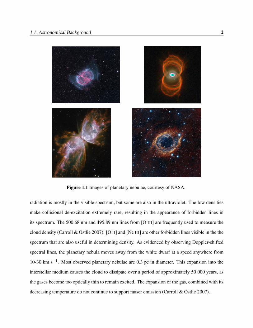
Planetary nebulae are the result of late stellar evolution in Aysmptotic Giant Branch (AGB)
stars. When fusionable materials run out in the interior of the star, the atmosphere is no longer
sustained by the pressure created by the reaction and collapses. The atmosphere rebounds off the
degenerate core and out into space. This material is the planetary nebula. The degenerate core
remains in its center as a white dwarf. The gases in the nebula are excited by constant radiation
from the white dwarf. As the electrons in the cloud cascade down energy levels, photons are
emitted. The low density of the cloud ensures that the majority of the photons escape. This
1
1.1 Astronomical Background 2
Figure 1.1 Images of planetary nebulae, courtesy of NASA.
radiation is mostly in the visible spectrum, but some are also in the ultraviolet. The low densities
make collisional de-excitation extremely rare, resulting in the appearance of forbidden lines in
its spectrum. The 500.68 nm and 495.89 nm lines from [O III] are frequently used to measure the
cloud density (Carroll & Ostlie 2007). [O II] and [Ne III] are other forbidden lines visible in the the
spectrum that are also useful in determining density. As evidenced by observing Doppler-shifted
spectral lines, the planetary nebula moves away from the white dwarf at a speed anywhere from
10-30 km s−1. Most observed planetary nebulae are 0.3 pc in diameter. This expansion into the
interstellar medium causes the cloud to dissipate over a period of approximately 50 000 years, as
the gases become too optically thin to remain excited. The expansion of the gas, combined with its
decreasing temperature do not continue to support maser emission (Carroll & Ostlie 2007).
1.2 Previous Work on K3-35 3
In relation to stellar atmospheres, maser radiation is only found in stellar envelopes of highly
evolved stars. The end processes of theses stars involves significant mass loss into the interstellar
medium. Late type AGB stars undergo this process as they gradually transform into planetary
nebulae. However, current astrophysical models are insufficient to explain the presence of maser
radiation in the evolved form of AGB stars.
1.2 Previous Work on K3-35
The target, PN K3-35, has been studied extensively in the past (Tafoya et al. 2007) (Gomez et al.
2009) (Tafoya et al. 2011). It is identified as a proto planetary nebula that experiences mass loss
in a torus around the equatorial region (Uscanga et al. 2008). There are also outflows at each of
the poles (Uscanga et al. 2008). At that time the peak flux in maser radiation was about 1572 mJy
(Uscanga et al. 2008). The torus has a rotational velocity of 3.1 km s−1 and expanding at a rate
of 1.4 km s−1 (Uscanga et al. 2008). Observation of the 22 GHz line reveals a systemic velocity
of 20.88 - 23.00 km s−1 in relation to the Local Standard of Rest (LSR) (Tafoya et al. 2011). Its
distance is estimated to be 5 kpc (Tafoya et al. 2011).
Hydroxyl (OH) masers were identified in 2009, at 1665 and 1720 MHz (Gomez et al. 2009).
They are distributed around the core of the nebula, while the previously observed water masers are
present in the outer envelope. Peak observed flux was 1496.6 mJy (Gomez et al. 2009).
Three H2O maser features detected in 2011 (Tafoya et al. 2011). More detailed observation in
infrared indicates that K3-35 has a total ionized mass of about 9x10⁻³ M� (Tafoya et al. 2007).
This total ionized material is inconsistent with known conditions for maser radiation.
1.3 Maser Physics 4
1.3 Maser Physics
The maser characteristics of astronomical hydroxyl maser emission were first observed in 1965.
Water maser emission was later observed by Cheung in 1969. Water masers were discovered to
be more compact in size and produce larger intensities than the hydroxyl masers (Carroll & Ostlie
2007). More complex molecules with maser properties were later discovered such as CH3OH and
SiO (Carroll & Ostlie 2007). Higher intensity radiation was then observed in the cores of galactic
nuclei and was classified as megamasers. Maser emission is from observed in star forming regions,
HII regions, supernova remnants, and stellar envelopes of stars.
Maser stands for Microwave Amplification by Stimulated Emission of Radiation. The term
has been colloquially shortened to "maser" just as the term laser. Microwaves are classified in
the radio regime of the electromagnetic spectrum. As such, masers are not limited microwaves,
but also included stimulated emission of radio waves. A maser functions similar to a laser in that
it is caused by stimulated emission when a population inversion occurs in molecular gas. The
energy transitions that occur involve changing rotational states within a molecule. These lower
energy transitions produce radio waves as opposed to visible light. The lower energy interactions
are observed frequently in nature, whereas laser emission has never been observed naturally by
account of its higher energy requirements. (Cohen 1989)
Maser radiation is not thermal in nature. This is significant because all other non radio sources
of astronomical radiation are caused by continuum radiation from a blackbody like object. Masers
are best described using the model of the three level atom. Incoming infrared photons serve as a
heating mechanism, pushing electrons in the water molecule into a higher rotational state. They
then decay into a slightly lower energy state. The second de-excitation is a result of spontaneous
emission, and the radio photon is emitted. Its interaction with a second molecule in the second
excited state causes stimulated emission, and a second radio photon is emitted with the same phase
and wavelength as the first. As this process repeats among the many molecules in a gas, there is a
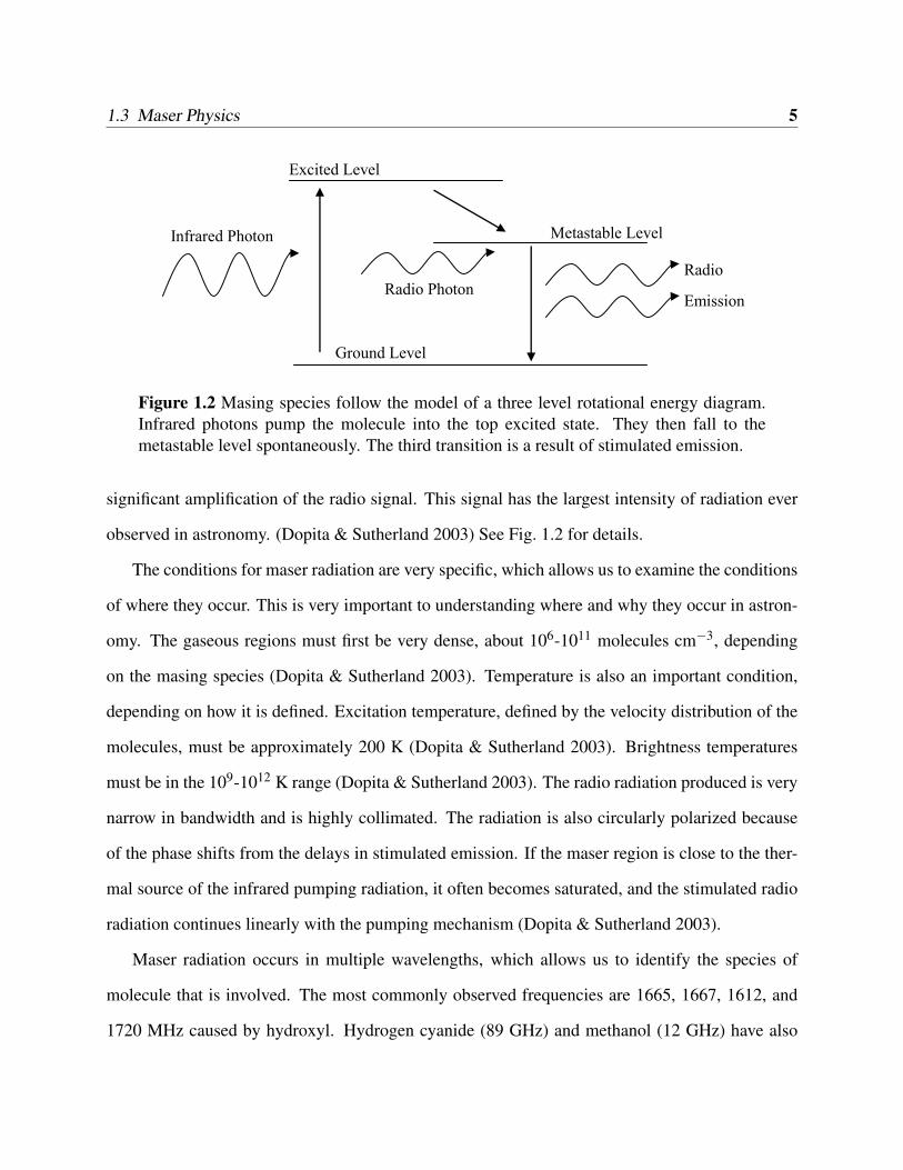
1.3 Maser Physics 5
Ground Level
Metastable Level
Excited Level
Infrared Photon
Radio
Emission Radio Photon
Figure 1.2 Masing species follow the model of a three level rotational energy diagram.Infrared photons pump the molecule into the top excited state. They then fall to themetastable level spontaneously. The third transition is a result of stimulated emission.
significant amplification of the radio signal. This signal has the largest intensity of radiation ever
observed in astronomy. (Dopita & Sutherland 2003) See Fig. 1.2 for details.
The conditions for maser radiation are very specific, which allows us to examine the conditions
of where they occur. This is very important to understanding where and why they occur in astron-
omy. The gaseous regions must first be very dense, about 106-1011 molecules cm−3, depending
on the masing species (Dopita & Sutherland 2003). Temperature is also an important condition,
depending on how it is defined. Excitation temperature, defined by the velocity distribution of the
molecules, must be approximately 200 K (Dopita & Sutherland 2003). Brightness temperatures
must be in the 109-1012 K range (Dopita & Sutherland 2003). The radio radiation produced is very
narrow in bandwidth and is highly collimated. The radiation is also circularly polarized because
of the phase shifts from the delays in stimulated emission. If the maser region is close to the ther-
mal source of the infrared pumping radiation, it often becomes saturated, and the stimulated radio
radiation continues linearly with the pumping mechanism (Dopita & Sutherland 2003).
Maser radiation occurs in multiple wavelengths, which allows us to identify the species of
molecule that is involved. The most commonly observed frequencies are 1665, 1667, 1612, and
1720 MHz caused by hydroxyl. Hydrogen cyanide (89 GHz) and methanol (12 GHz) have also
1.4 Overview 6
been observed in star forming regions.
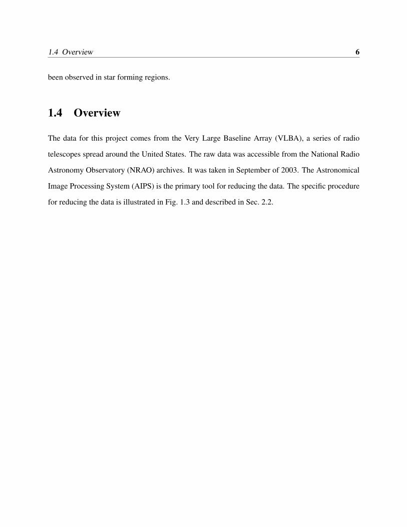
1.4 Overview
The data for this project comes from the Very Large Baseline Array (VLBA), a series of radio
telescopes spread around the United States. The raw data was accessible from the National Radio
Astronomy Observatory (NRAO) archives. It was taken in September of 2003. The Astronomical
Image Processing System (AIPS) is the primary tool for reducing the data. The specific procedure
for reducing the data is illustrated in Fig. 1.3 and described in Sec. 2.2.
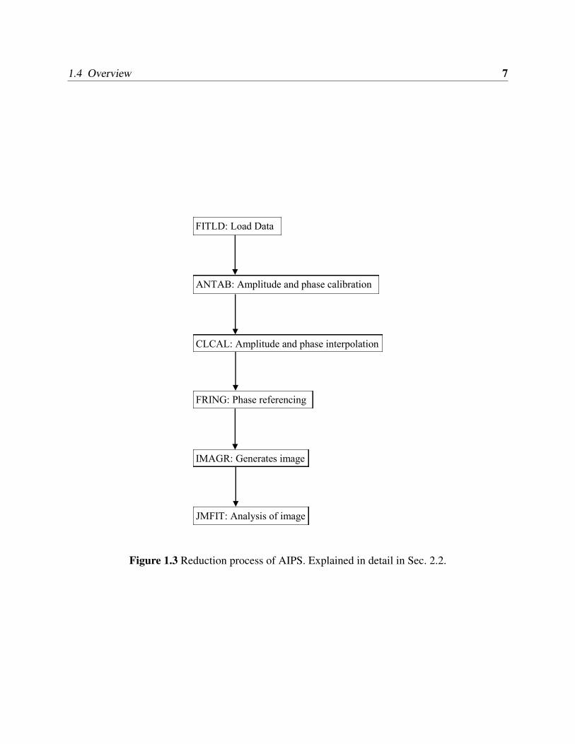
1.4 Overview 7
FITLD: Load Data
ANTAB: Amplitude and phase calibration
CLCAL: Amplitude and phase interpolation
FRING: Phase referencing
IMAGR: Generates image
JMFIT: Analysis of image
Figure 1.3 Reduction process of AIPS. Explained in detail in Sec. 2.2.
Chapter 2
Observations And Data Reduction
2.1 Radio Telescopes
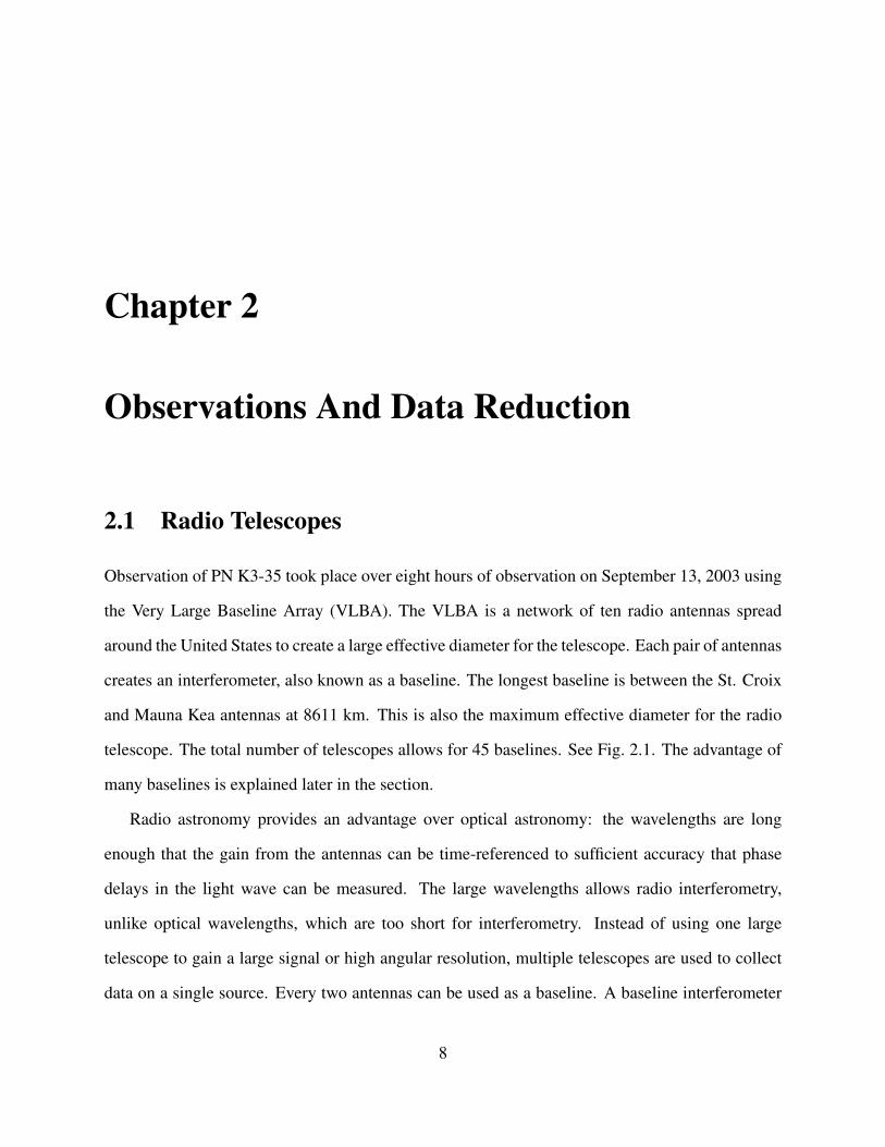
Observation of PN K3-35 took place over eight hours of observation on September 13, 2003 using
the Very Large Baseline Array (VLBA). The VLBA is a network of ten radio antennas spread
around the United States to create a large effective diameter for the telescope. Each pair of antennas
creates an interferometer, also known as a baseline. The longest baseline is between the St. Croix
and Mauna Kea antennas at 8611 km. This is also the maximum effective diameter for the radio
telescope. The total number of telescopes allows for 45 baselines. See Fig. 2.1. The advantage of
many baselines is explained later in the section.
Radio astronomy provides an advantage over optical astronomy: the wavelengths are long
enough that the gain from the antennas can be time-referenced to sufficient accuracy that phase
delays in the light wave can be measured. The large wavelengths allows radio interferometry,
unlike optical wavelengths, which are too short for interferometry. Instead of using one large
telescope to gain a large signal or high angular resolution, multiple telescopes are used to collect
data on a single source. Every two antennas can be used as a baseline. A baseline interferometer
8
2.1 Radio Telescopes 9
Figure 2.1 Map of the VLBA, courtesy of NRAO.
is similar to the double-slit interferometer. In this setup, a plane wave from a distant source is
incoming on a double slit, or in this case, the two antennas of a baseline. The signal obtained from
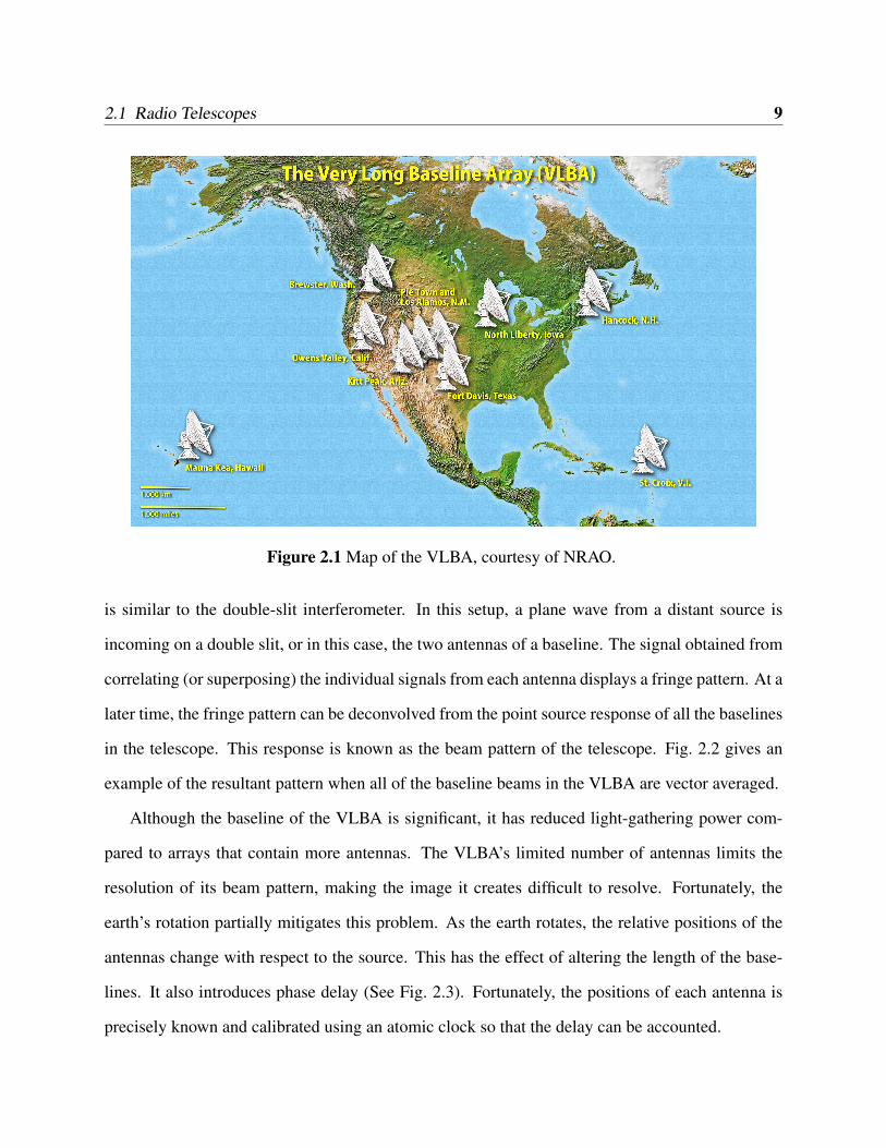
correlating (or superposing) the individual signals from each antenna displays a fringe pattern. At a
later time, the fringe pattern can be deconvolved from the point source response of all the baselines
in the telescope. This response is known as the beam pattern of the telescope. Fig. 2.2 gives an
example of the resultant pattern when all of the baseline beams in the VLBA are vector averaged.
Although the baseline of the VLBA is significant, it has reduced light-gathering power com-
pared to arrays that contain more antennas. The VLBA’s limited number of antennas limits the
resolution of its beam pattern, making the image it creates difficult to resolve. Fortunately, the
earth’s rotation partially mitigates this problem. As the earth rotates, the relative positions of the
antennas change with respect to the source. This has the effect of altering the length of the base-
lines. It also introduces phase delay (See Fig. 2.3). Fortunately, the positions of each antenna is
precisely known and calibrated using an atomic clock so that the delay can be accounted.
2.1 Radio Telescopes 10
Figure 2.2 Beam pattern for the VLBA. It is constructed by convolving the beams of eachof the antennas in the array over the course of observation. This beam pattern is used toremove the fringe pattern in the VLBA’s image.
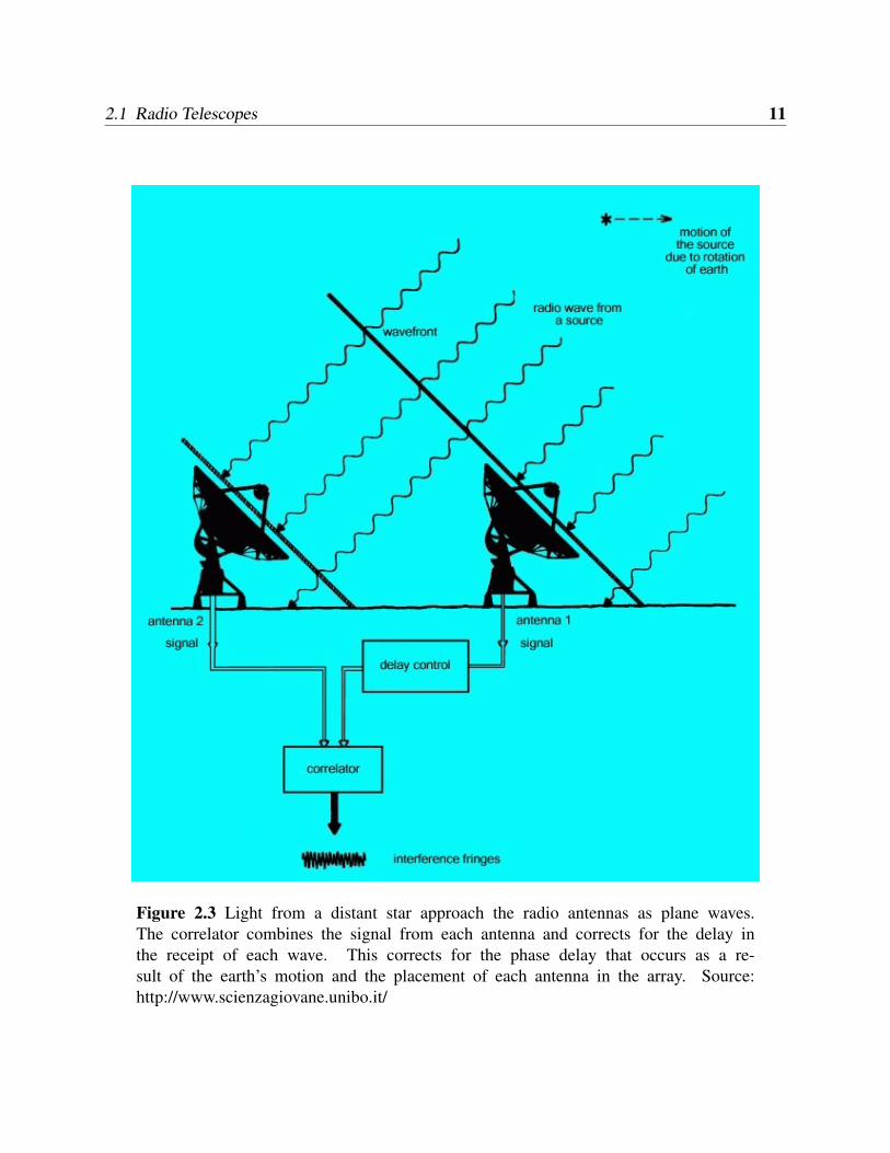
2.1 Radio Telescopes 11
Figure 2.3 Light from a distant star approach the radio antennas as plane waves.The correlator combines the signal from each antenna and corrects for the delay inthe receipt of each wave. This corrects for the phase delay that occurs as a re-sult of the earth’s motion and the placement of each antenna in the array. Source:http://www.scienzagiovane.unibo.it/
2.1 Radio Telescopes 12
Meg
a W
avln
gth
Mega Wavlngth400 300 200 100 0 -100 -200 -300 -400 -500
300
200
100
0
-100
-200
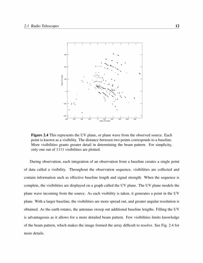
Figure 2.4 This represents the UV plane, or plane wave from the observed source. Eachpoint is known as a visibility. The distance between two points corresponds to a baseline.More visibilities grants greater detail in determining the beam pattern. For simplicity,only one out of 1111 visibilities are plotted.
During observation, each integration of an observation from a baseline creates a single point
of data called a visibility. Throughout the observation sequence, visibilities are collected and
contain information such as effective baseline length and signal strength. When the sequence is
complete, the visibilities are displayed on a graph called the UV plane. The UV plane models the
plane wave incoming from the source. As each visibility is taken, it generates a point in the UV
plane. With a larger baseline, the visibilities are more spread out, and greater angular resolution is
obtained. As the earth rotates, the antennas sweep out additional baseline lengths. Filling the UV
is advantageous as it allows for a more detailed beam pattern. Few visibilities limits knowledge
of the beam pattern, which makes the image formed the array difficult to resolve. See Fig. 2.4 for
more details.
2.2 AIPS Reduction 13
An antenna in an array is simply a point detector. Only radio flux (or signal) is measured by
each antenna. The convolution of each antenna’s signal to the visibilities in the UV plane generate
the image of the source. Once the image is obtained, it must be deconvolved with the previously
determined beam pattern of the array. This is done using phase reference data, obtained by either
observing a standard continuum source, or by using reduction software to model potential source
types to deconvolved the image one step at a time. See Fig. 2.2.
2.2 AIPS Reduction
2.2.1 Loading Data
The standard tool for reducing radio data for the National Radio Astronomy Observatory (NRAO)
is the Astronomical Image Processing System (AIPS). AIPS is available to use on Linux operating
systems and was provided by Brigham Young University as a courtesy. The data from PN K3-35
comes from the NRAO archive. It is now part of the public domain.
Raw data is stored in image files called fits (with the extension .fits), as is standard for the
NRAO. .fits files, however, are limited in size and must be uploaded in several stages. Data on PN
K3-35 was included in eight .fits files. The data was uploaded into AIPS with the fitload (FITLD)
task. Once it was uploaded, it was concatenated using a task that sorts the data with respect to time
of observation (UVSRT). UVSRT references the time table of the data set to order the observations.
2.2.2 Corrections to the Data
Each antenna in the area is different and is subjected to differing atmospheric and ionospheric
conditions. To account for the differences, each antenna records its temperature, gain, and phase
characteristics, which are appended to the .fits files in calibration tables. An important calibration
table is the flag (FG) table. This table contains information about various errors that occur during
2.2 AIPS Reduction 14
observation, such as malfunctioning mounts and errors in phase data. This table is used to eliminate
bad visibilities from the data set without erasing the visibilities themselves. Once the reduction is
complete, all the calibration tables are applied to the data set to create the solution.
Another table includes the system temperature of each antenna. The response of an individual
antenna to the incoming signal is the gain. Temperature predictably affects the gain of each antenna
depending on the wavelength that is being observed. The array was set to observed 22 GHz line
emission, so appropriate gain correction was applied.
The SN table from the data set contains the positions of the antennas and thus their phase delay
information. It also contains data on the gain for each antenna. The task ANTAB applies the
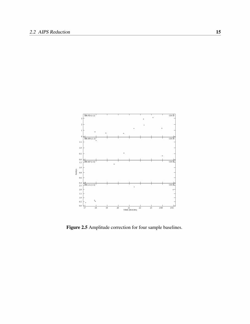
amplitude correction for each antenna. Fig. 2.5 gives examples of the amplitude data for four of
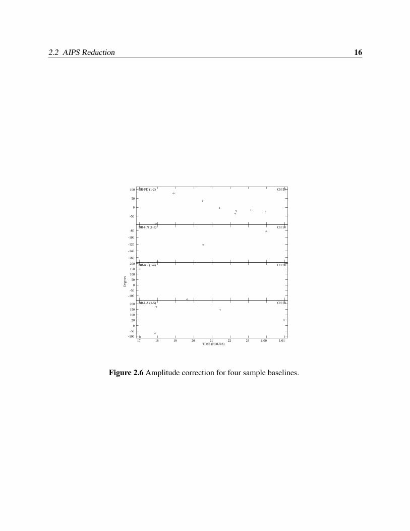
the baselines in the array. ANTAB also corrects the phase delay in each of the baselines. Fig. 2.6
gives examples of the phase correction data for four of the baselines.
The correctional data, however, is not immediately applied to the data set. Instead, it is stored
in a calibration table (CL). The amplitude and phase information tables are limited. Not every
visibility has a corresponding phase delay or amplitude correction. This leaves large gaps in
the calibration for the visibilities that are not labeled. Applying the calibration correction task
(CLCAL) to the unlabeled visibilities uses linear interpolation to approximate the amplitude and
phase information across the gaps.
The baseline length data contained in each visibility can be plotted. The result is Fig. 2.4.
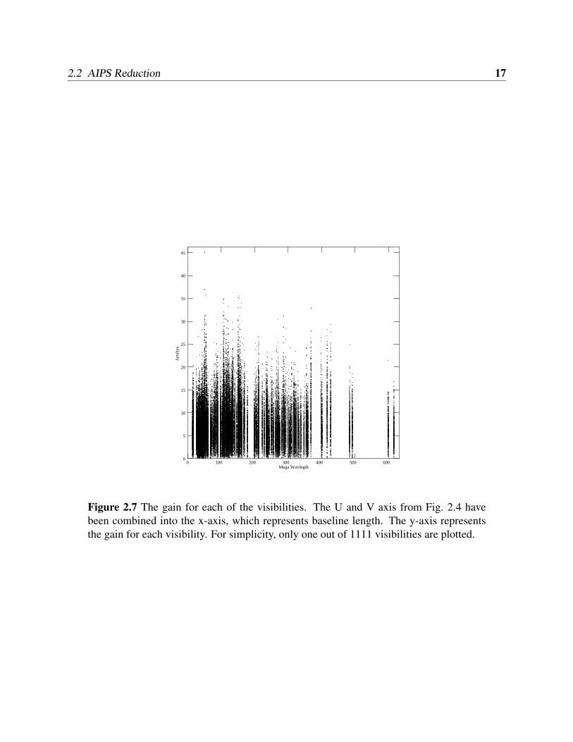
The gain of each visibility can also be compared with baseline length (Fig. 2.7). Any outlying
visibilities in the data can be added to FG table so that it can be ignored in the final solution. In
this data set, all visibilities with a signal over 40 Jy were added to the FG table.
2.2 AIPS Reduction 15
3
2
1
0
BR-FD (1-2) CH 50
1.5
1.0
0.5
0.0
BR-HN (1-3) CH 50
Jans
kys
1.2
1.0
0.8
0.6
0.4
BR-KP (1-4) CH 50
TIME (HOURS)17 18 19 20 21 22 23 1/00 1/01
2.5
2.0
1.5
1.0
0.5
0.0
BR-LA (1-5) CH 50
Figure 2.5 Amplitude correction for four sample baselines.
2.2 AIPS Reduction 16
100
50
0
-50
BR-FD (1-2) CH 50
-80
-100
-120
-140
-160
BR-HN (1-3) CH 50
Deg
rees
200
150
100
50
0
-50
-100
BR-KP (1-4) CH 50
TIME (HOURS)17 18 19 20 21 22 23 1/00 1/01
200
150
100
50
0
-50
-100
BR-LA (1-5) CH 50
Figure 2.6 Amplitude correction for four sample baselines.
2.2 AIPS Reduction 17
Jans
kys
Mega Wavlngth0 100 200 300 400 500 600
45
40
35
30
25
20
15
10
5
0
Figure 2.7 The gain for each of the visibilities. The U and V axis from Fig. 2.4 havebeen combined into the x-axis, which represents baseline length. The y-axis representsthe gain for each visibility. For simplicity, only one out of 1111 visibilities are plotted.
2.2 AIPS Reduction 18
2.2.3 Creating a Solution
Most radio arrays have multiple frequency channels (IF). The VLBA has two, so that two different
wavelengths can be observed at the same time. The observation was only conducted on the 22 GHz
emission line, so only one IF was required. However, polarization data was initially included in the
separate IF channel. This was a mistake. We had to return to the FITLD task, reload the data into
AIPS, and resort the data using the indexing and sorting tasks to append the data into the correct
tables. Otherwise, the polarization of the radio wave would have interfered with the calibrated data
set.
Each antenna in the array contains 256 channels. These channels sweep through electromag-
netic spectrum in the 22 GHz range in small intervals to create a spectrum of the target. The
spectrum difference is due to doppler shift based on the velocity of the target. Thus relative veloc-
ity is determined from the spectra of K3-35. This slices the target into discrete velocity intervals
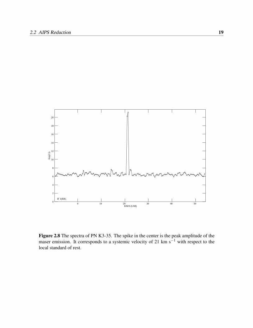
which are used to create a three dimensional greyscale image of the target. See Fig 2.8. The veloc-
ity was calibrated by using the same systemic velocity that was previously measured (Tafoya et al.
2011). The peak wavelength is centered on 21 km s−1.
Amplitude calibration data is obtained by observing a standard continuum source of radio
radiation (The standard used for this observation was J1925+2106). The standard has a well known
constant flux in all channels. The data obtained from K3-35 has flux determined from the antenna
gain, but does not account for interstellar or atmospheric absorbtion. By measuring the flux from
the standard star just prior to observing the target, a scale factor for the losses is obtained. The
scale factor is then applied to flux from PN K3-35 to obtain the true flux from the object.
Standard stars can also be used for finding good positions and improve sensitivity. This helps
reduce the side lobes and noise level before considering self-calibration. Unfortunately, no phase
referenced standard was provided with the data, necessitating the self-calibration described in
Sec. 2.2.4.
2.2 AIPS Reduction 19
Am
pl J
y
KM/S (LSR)0 10 20 30 40 50
20
18
16
14
12
10
8
6
4
2
0IF 1(RR)
Figure 2.8 The spectra of PN K3-35. The spike in the center is the peak amplitude of themaser emission. It corresponds to a systemic velocity of 21 km s−1 with respect to thelocal standard of rest.
2.2 AIPS Reduction 20
AIPS includes the fringe calibration task (FRING). This task attempts to improve the phase
info by finely defining the fringe rate and delay in the generated image. The absence of phase
referenced data hampers this task. This calibration does not better the reduced image of PN K3-
35, so I have rejected the FRING calibration.
Once these calibration steps are complete, the calibration tables need to be applied to the data
set. The task labeled CVEL splits the calibration table to the existing data and generates a new file
for reduced data. This can be treated as a separate object from the original data. Thus the original
data is preserved in case more correction is necessary.
2.2.4 Self-Calibration
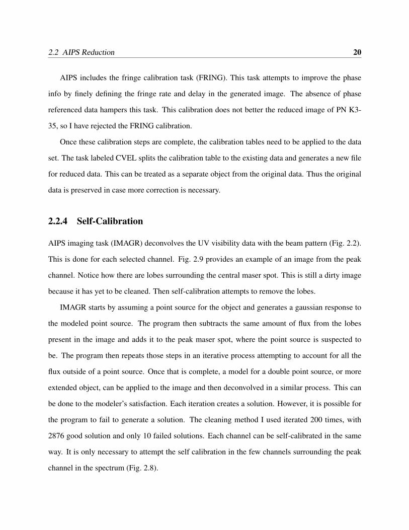
AIPS imaging task (IMAGR) deconvolves the UV visibility data with the beam pattern (Fig. 2.2).
This is done for each selected channel. Fig. 2.9 provides an example of an image from the peak
channel. Notice how there are lobes surrounding the central maser spot. This is still a dirty image
because it has yet to be cleaned. Then self-calibration attempts to remove the lobes.
IMAGR starts by assuming a point source for the object and generates a gaussian response to
the modeled point source. The program then subtracts the same amount of flux from the lobes
present in the image and adds it to the peak maser spot, where the point source is suspected to
be. The program then repeats those steps in an iterative process attempting to account for all the
flux outside of a point source. Once that is complete, a model for a double point source, or more
extended object, can be applied to the image and then deconvolved in a similar process. This can
be done to the modeler’s satisfaction. Each iteration creates a solution. However, it is possible for
the program to fail to generate a solution. The cleaning method I used iterated 200 times, with
2876 good solution and only 10 failed solutions. Each channel can be self-calibrated in the same
way. It is only necessary to attempt the self calibration in the few channels surrounding the peak
channel in the spectrum (Fig. 2.8).
2.2 AIPS Reduction 21
GREY: K3-35 IPOL 22234.294 MHZ CHAN132IMG.IMAG.1PLot file version 1 created 30-MAR-2012 08:23:16
Grey scale flux range= -0.074 0.959 JY/BEAM
0.0 0.2 0.4 0.6 0.8
DE
CL
INA
TIO
N (
J200
0)
RIGHT ASCENSION (J2000)19 27 44.0245 44.0240 44.0235 44.0230
21 30 03.465
03.460
03.455
03.450
03.445
03.440
Figure 2.9 Image of the source for the peak flux channel.
2.2 AIPS Reduction 22
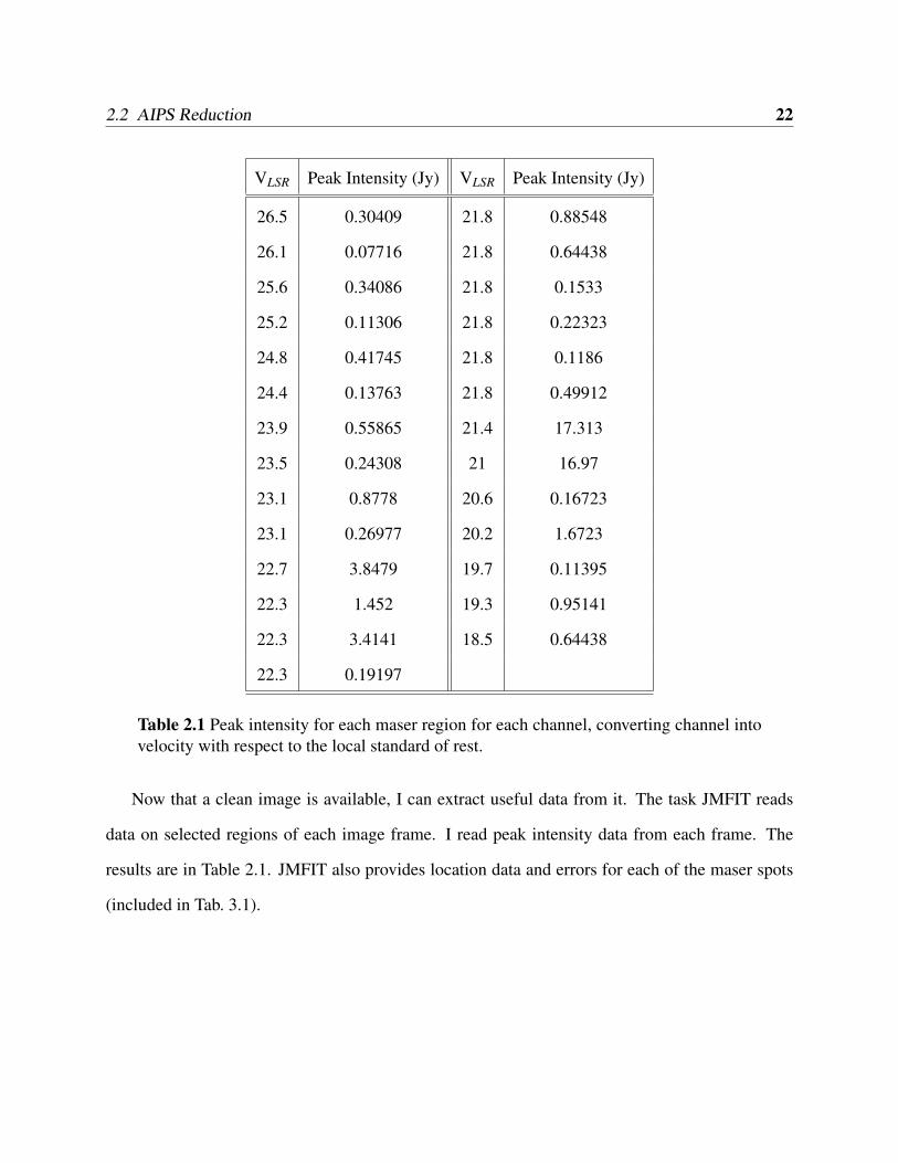
VLSR Peak Intensity (Jy) VLSR Peak Intensity (Jy)
26.5 0.30409 21.8 0.88548
26.1 0.07716 21.8 0.64438
25.6 0.34086 21.8 0.1533
25.2 0.11306 21.8 0.22323
24.8 0.41745 21.8 0.1186
24.4 0.13763 21.8 0.49912
23.9 0.55865 21.4 17.313
23.5 0.24308 21 16.97
23.1 0.8778 20.6 0.16723
23.1 0.26977 20.2 1.6723
22.7 3.8479 19.7 0.11395
22.3 1.452 19.3 0.95141
22.3 3.4141 18.5 0.64438
22.3 0.19197
Table 2.1 Peak intensity for each maser region for each channel, converting channel intovelocity with respect to the local standard of rest.
Now that a clean image is available, I can extract useful data from it. The task JMFIT reads
data on selected regions of each image frame. I read peak intensity data from each frame. The
results are in Table 2.1. JMFIT also provides location data and errors for each of the maser spots
(included in Tab. 3.1).
Chapter 3
Discussion
3.1 Analysis
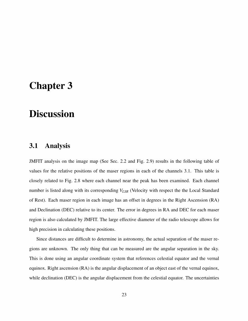
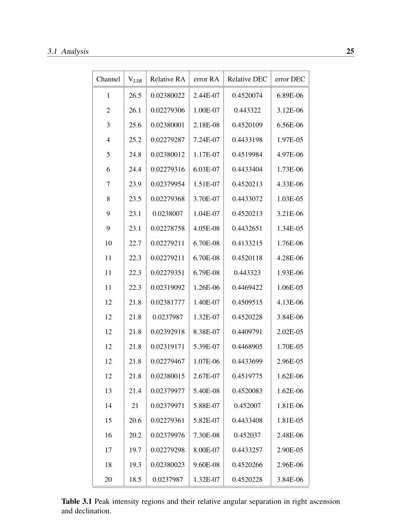
JMFIT analysis on the image map (See Sec. 2.2 and Fig. 2.9) results in the following table of
values for the relative positions of the maser regions in each of the channels 3.1. This table is
closely related to Fig. 2.8 where each channel near the peak has been examined. Each channel
number is listed along with its corresponding VLSR (Velocity with respect the the Local Standard
of Rest). Each maser region in each image has an offset in degrees in the Right Ascension (RA)
and Declination (DEC) relative to its center. The error in degrees in RA and DEC for each maser
region is also calculated by JMFIT. The large effective diameter of the radio telescope allows for
high precision in calculating these positions.
Since distances are difficult to determine in astronomy, the actual separation of the maser re-
gions are unknown. The only thing that can be measured are the angular separation in the sky.
This is done using an angular coordinate system that references celestial equator and the vernal
equinox. Right ascension (RA) is the angular displacement of an object east of the vernal equinox,
while declination (DEC) is the angular displacement from the celestial equator. The uncertainties
23
3.1 Analysis 24
in each of the of the maser positions are included. The errors in RA and DEC can be examined
while the error in velocity space is insignificant. If the separation of two maser regions is less than
the calculated error, they can be safely assumed to be part of the same maser region.
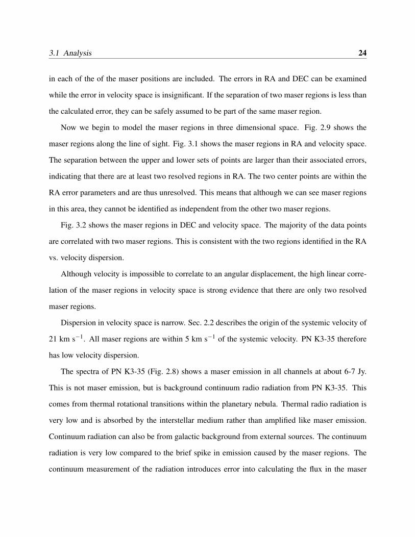
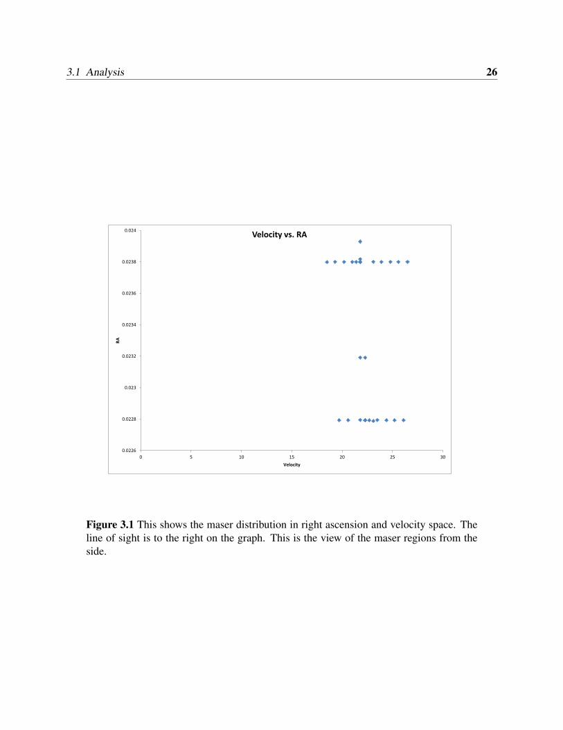
Now we begin to model the maser regions in three dimensional space. Fig. 2.9 shows the
maser regions along the line of sight. Fig. 3.1 shows the maser regions in RA and velocity space.
The separation between the upper and lower sets of points are larger than their associated errors,
indicating that there are at least two resolved regions in RA. The two center points are within the
RA error parameters and are thus unresolved. This means that although we can see maser regions
in this area, they cannot be identified as independent from the other two maser regions.
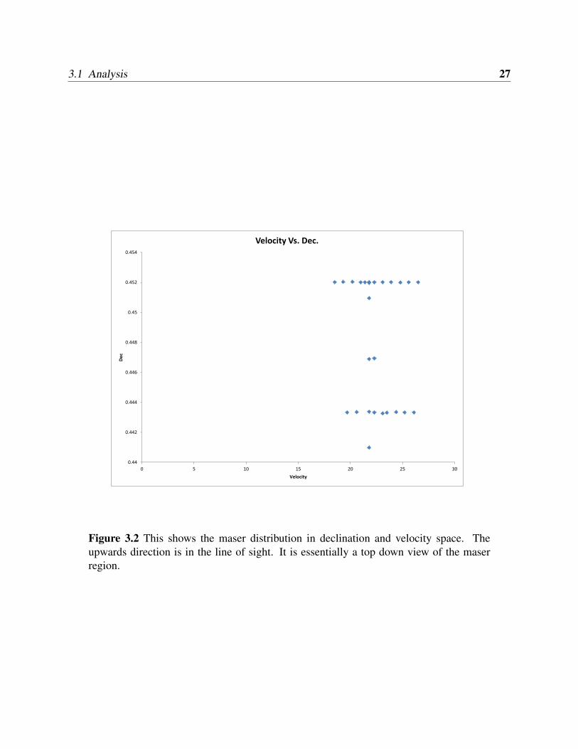
Fig. 3.2 shows the maser regions in DEC and velocity space. The majority of the data points
are correlated with two maser regions. This is consistent with the two regions identified in the RA
vs. velocity dispersion.
Although velocity is impossible to correlate to an angular displacement, the high linear corre-
lation of the maser regions in velocity space is strong evidence that there are only two resolved
maser regions.
Dispersion in velocity space is narrow. Sec. 2.2 describes the origin of the systemic velocity of
21 km s−1. All maser regions are within 5 km s−1 of the systemic velocity. PN K3-35 therefore
has low velocity dispersion.
The spectra of PN K3-35 (Fig. 2.8) shows a maser emission in all channels at about 6-7 Jy.
This is not maser emission, but is background continuum radio radiation from PN K3-35. This
comes from thermal rotational transitions within the planetary nebula. Thermal radio radiation is
very low and is absorbed by the interstellar medium rather than amplified like maser emission.
Continuum radiation can also be from galactic background from external sources. The continuum
radiation is very low compared to the brief spike in emission caused by the maser regions. The
continuum measurement of the radiation introduces error into calculating the flux in the maser
3.1 Analysis 25
Channel VLSR Relative RA error RA Relative DEC error DEC
1 26.5 0.02380022 2.44E-07 0.4520074 6.89E-06
2 26.1 0.02279306 1.00E-07 0.443322 3.12E-06
3 25.6 0.02380001 2.18E-08 0.4520109 6.56E-06
4 25.2 0.02279287 7.24E-07 0.4433198 1.97E-05
5 24.8 0.02380012 1.17E-07 0.4519984 4.97E-06
6 24.4 0.02279316 6.03E-07 0.4433404 1.73E-06
7 23.9 0.02379954 1.51E-07 0.4520213 4.33E-06
8 23.5 0.02279368 3.70E-07 0.4433072 1.03E-05
9 23.1 0.0238007 1.04E-07 0.4520213 3.21E-06
9 23.1 0.02278758 4.05E-08 0.4432651 1.34E-05
10 22.7 0.02279211 6.70E-08 0.4133215 1.76E-06
11 22.3 0.02279211 6.70E-08 0.4520118 4.28E-06
11 22.3 0.02279351 6.79E-08 0.443323 1.93E-06
11 22.3 0.02319092 1.26E-06 0.4469422 1.06E-05
12 21.8 0.02381777 1.40E-07 0.4509515 4.13E-06
12 21.8 0.0237987 1.32E-07 0.4520228 3.84E-06
12 21.8 0.02392918 8.38E-07 0.4409791 2.02E-05
12 21.8 0.02319171 5.39E-07 0.4468905 1.70E-05
12 21.8 0.02279467 1.07E-06 0.4433699 2.96E-05
12 21.8 0.02380015 2.67E-07 0.4519775 1.62E-06
13 21.4 0.02379977 5.40E-08 0.4520083 1.62E-06
14 21 0.02379971 5.88E-07 0.452007 1.81E-06
15 20.6 0.02279361 5.82E-07 0.4433408 1.81E-05
16 20.2 0.02379976 7.30E-08 0.452037 2.48E-06
17 19.7 0.02279298 8.00E-07 0.4433257 2.90E-05
18 19.3 0.02380023 9.60E-08 0.4520266 2.96E-06
20 18.5 0.0237987 1.32E-07 0.4520228 3.84E-06
Table 3.1 Peak intensity regions and their relative angular separation in right ascensionand declination.
3.1 Analysis 26
0.0226
0.0228
0.023
0.0232
0.0234
0.0236
0.0238
0.024
0 5 10 15 20 25 30
RA
Velocity
Velocity vs. RA
Figure 3.1 This shows the maser distribution in right ascension and velocity space. Theline of sight is to the right on the graph. This is the view of the maser regions from theside.
3.1 Analysis 27
0.44
0.442
0.444
0.446
0.448
0.45
0.452
0.454
0 5 10 15 20 25 30
De
c
Velocity
Velocity Vs. Dec.
Figure 3.2 This shows the maser distribution in declination and velocity space. Theupwards direction is in the line of sight. It is essentially a top down view of the maserregion.

3.1 Analysis 28
regions. The distribution is flat, which fortunately minimizes the error. Running JMFIT in the non
masing regions of Fig. 2.9 reveals that the mean value of the radiation in those areas is uniform
and constant.
Chapter 4
Conclusions
4.1 Results
Only two maser regions in PN K3-35 have been resolved using the VLBA data. Later observations
from Uscanga (Uscanga et al. 2008) and Tafoya (Tafoya et al. 2007) using multiple single dish
telescopes show more masing regions and at a lower intensity. It is likely that there are indeed
more maser regions than the two observed here. The limiting factor is the sensitivity of the VLBA,
which is limited to ten antennas. Further observations were conducted using the VLA, which has
greater sensitivity while sacrificing resolution (See Sec. 2.1). Also, the beam from the VLBA is
very small and has washed out the weaker and non-compact maser emission in the medium.
Decreases in the intensity of the radiation from the target were observed previously (Uscanga
et al. 2008) (Tafoya et al. 2007). Their measurements are in the milliJansky range. This is consis-
tent with stellar evolution models that maser regions disappear when a late type star transitions into
a planetary nebula. However, the mere presence of maser emission is evidence that PN K3-35 is
not a planetary nebula. Instead it suggests that PN K3-35 is still partly a late type star, even though
optical and infrared data identify it as a planetary nebula. The evolution of the region is unknown.
29
4.2 Directions for Further Work 30
The two spots that are resolved are insufficient to model mass flow from the region. All that
we can conclude is that the masers indicate the presence of water in the stellar atmosphere. While
it is possible for maser radiation exist within the region, the required conditions are not directly
observed. However, the mere presence of maser infers the existence of those conditions in the
region.
4.2 Directions for Further Work
Further study of PN K3-35 is needed to model the expansion of the maser regions in the interstellar
medium. While it is reasonable to assume that the maser regions will weaken as the gas expands,
the radiation is at a high enough intensity to expect it to be observable for many more years.
However, as the physics of the region are still not well understood, the timescale for the decrease
in maser radiation to below a detectable level is unknown. Our best estimate is that the radiation
will only last a couple more decades. Tracking the proper motion of the maser regions will allow
for the determination of size and rate of expansion once better estimates of distance have been
obtained. Observations of the decrease in maser intensity can also help build models for what is
causing the maser radiation and the expansion of the shell.
PN K3-35 is also a prototype for identifying other planetary nebulae with maser emission.
While PN K3-35 is the only identified object of its kind, we speculate that it is unlikely to be the
only one. New radio telescope arrays such as the Square Kilometer Array (SKA) under construc-
tion will allow for greater sensitivity in searching for weak maser emission in distant targets. Also,
new advances in information technology have started a new area of astronomy called astroinfor-
matics. This will involve collecting and correlating large amounts of data from all-sky surveys,
improving current data mining techniques. This can be done with optical and infrared data and
then quickly referenced with existing radio data (as well as standard monitoring of continuum ra-

4.2 Directions for Further Work 31
dio background) to identify other planetary nebulae with maser characteristics. Once identified,
these targets can be observed in detail using the more powerful instruments of SKA and ALMA.
The additional data will be helpful in creating models for PN K3-35 and other planetary nebulae.

Bibliography
Carroll, B. W., & Ostlie, D. A. 2007, An Introduction to Modern Astrophysics, 2nd edn. (San
Fransisco: Wiley), 470
Cohen, R. 1989, Reports on Progress in Physics, 52, 881
Dopita, M. A., & Sutherland, R. S. 2003, Astrophysics of the Diffuse Universe, 2nd edn. (Springer-
Verlag Berlin Heidelberg: Springer), 88
Gomez, Y., Tafoya, D., & Anglada, G. 2009, Astrophysical Journal, 695, 930
Tafoya, D., Gomez, Y., & Anglada, G. 2007, Astronomical Journal, 133, 364
Tafoya, D., Imai, H., & Gomez, Y. 2011, Astronomical Society of Japan, 63, 71
Uscanga, L., Gomez, Y., & Raga, A. 2008, Monthly Notices of the Royal Astronomical Society,
390, 1127
32

Index
amplitude, 14, 18
baseline, 8, 9, 14beam pattern, 9, 12, 20
continuum radiation, 24
declination, 23, 24
flux, 3, 18, 20
interstellar medium, 3, 24, 30
maser, 2, 3, 22, 24conditions, 5, 30hydroxyl, 3, 5mechanism, 4, 5water, 3–5, 30
outlow, 3
phase delay, 8, 9, 18, 20planetary nebula, 1, 3, 24, 29, 30
right ascension, 23, 24
temperaturebrightness, 5kinetic, 2system, 14
torus, 3
velocityBoltzmann distribution, 5local standard of rest, 3, 23relative, 18, 24systemic, 18, 24
visibility, 12–14
VLBA, 6, 8, 9, 29
white dwarf, 1
33


![IPD/Bim Thesis Proposal - engr.psu.edu · [IPD/BIM THESIS PROPOSAL] Jason Brognano, Michael Gilroy, Stephen Kijak, David Maser December 6, 2010 KGB Maser KGB Maser| BIM/IPD Thesis](https://img.pdfslide.us/doc/110x75/605d339025f9181d960e06e8/ipdbim-thesis-proposal-engrpsuedu-ipdbim-thesis-proposal-jason-brognano.jpg)