NONLINEAR OBSERVERS FOR GYRO CALIBRATION COUPLED WITH A NONLINEAR CONTROL ALGORITHM

Julie Thienel* and Robert M. Sannert

Nonlinear observers for gyro calibration are presented. The first observer esti- mates a constant gyro bias. The second observer estimates scale factor errors. The third observer estimates the gyro alignment for three orthogonal gyros. The observers are then combined. The convergence properties of all three observers, and the combined observers, are discussed. Additionally, all three observers are coupled with a nonlinear control algorithm. The stability of each of the resulting closed loop systems is analyzed. Simulated test results are presented for each system.

INTRODUCTION

Gyroscopes, also known as Inertial Reference Units (IRU) or gyros, are part of the attitude control system of most three-axis stabilized spacecraft. They measure the spacecraft angular rate. Unfortu- nately, the gyro measurements axe corrupted by errors in alignment, scale factor, and bias, as well as :ando=; noise.' Sevsrd dgoiithiiis G i astiiiiaiing iiie errors, as weii as the noise characteristics, are available.2-8 Most algorithms rely on linear techniques and are not coupled directly with the spacecraft control.

The published nonlinear methods tend to follow a similar Lyapunov development to determine stability, most are driven by a measurable attitude error. Alonso, et al. in Ref. 9 develop a nonlinear observer for relative attitude and rate estimation with an application to spacecraft formation flying. Salcudean in Ref. 10 develops a nonlinear observer for angular rate estimation. Both observers are driven by a computed attitude error. However, in order to estimate the rate, both observers require knowledge or estimation of spacecraft torques. The stability of the observer developed by Salcudean requires an assumption that the system eventually behaves as a linear time invariant system. In Ref. 11, Vik, et al. develop an angular velocity observer, in addition to a position and velocity observer, for use in a Global Positioning System (GPS)/Inertial Navigation System (INS). The angular velocity observer is actually a nonlinear observer for gyro calibration. The observer is designed to estimate corrections to the gyro measurements, particularly misalignment and scale factor corrections, along with gyro biases. The misalignment and scale factor errors are assumed to be small. All the error terms are modelled as exponentially decaying, first-order equations. The Lyapunov analysis proves that the observer, given the above assumptions, is exponentially stable. A closed-loop analysis of the observer, coupled with a controller, is not presented. Nonlinear observers for gyro bias estimation are presented by Boskovic, et al. in Refs. 12 and 13. In Ref. 12, the bias is assumed to be constant, which differs from the exponentially decaying model of Ref. 11. However, the bias is assumed to lie in a small, bounded set. Second order terms are neglected in the observer development and in the Lyapunov proof of stability. The observer is coupled with a controller which is designed to drive the spacecraft rates to zero and the spacecraft body coordinates to the inertial coordinates. With the second order terms neglected, the closed loop system is stable for the single scenario presented. In RRf. 13, the gyro bias observer is designed for use in attitude tracking. Here the bias observer is driven by a computed attitude error, as in Refs. 9, 10, and 11. However, the attitude error is computed as a

*NASA Goddard Space Flight Center, Flight Dynamics Analysis Branch, Greenbelt, MD 20771, phone: 301-286-9033,

tuniversity of Maryland, Department of Aerospace Engineering, College Park, Maryland, 20742 phone: 301-405-1928, fax: 301-286-0369, email: julie.thienelQnasa.gov

fax: 301-314-9001, email: rmsannerOeng.umd.edu

1

https://ntrs.nasa.gov/search.jsp?R=20040016381 2018-07-03T06:27:43+00:00Z

vector difference, rather than a rotational error, without consideration to the normality constraint of the attitude. An adaptive tracking controller is coupled to the observer. The convergence proof for this observer assumes that the vehicle attitude never passes through zk180 degrees, and the stability of the coupled observer/controller/spacecraft dynamics is not formally established.

As the above discussion indicates, combined observer-controller designs for the attitude control of rigid flight vehicles are a subject of active ~-esearch.l'-'~ Successful design of such architectures is complicated by the fact that there is, in general, no separation principle for nonlinear systems. In contrast to linear systems, 'certainty equivalence' substitution of the states from an exponentially con- verging observer into a nominally stabilizing, state feedback control law does not necessarily guarantee stable closed-loop operation for the coupled systems.14> l5 In this work, one version of this problem is considered, the task of forcing the attitude of a rigid vehicle to asymptotically track a (time-varying) reference attitude using feedback from rate sensors with persistent nonzero errors.

The next section introduces the terminology used throughout the document, as well as an overview of a nonlinear attitude control law. Next, the development of nonlinear observers for the case of constant gyro bias, constant scale factor error, and constant alignment error are presented. Each observer is combined with the nonlinear control scheme for attitude control of a spacecraft. Simulation results are presented for each of the observers and for each of the closed loop systems. The paper concludes with a summary and discussion of future work.

TERMINOLOGY

The a.ttitude of B spcecr& Ca.2 be represelltete:! by 3 q.d%t.terrion consisting of a rotatioii aiigk and unit rotation vector e, known as the Euler axis, and a rotation q5 about this axis so that16

e sin(&) 4 = [ cos({) I = [ f 1

where q is the quaternion, partitioned into a vector part, E , and a scalar part, q. Typically, in spacecraft attitude applications, the quaternion represents the rotation from an inertial coordinate system to the spacecraft body coordinate system. Note that 1 lqll = 1 by definition. The rotation matrix for a specific attitude can be computed from the quaternion components as R(q) = (q2 -~T~) I+2~~T-27$ ' (~ ) where I is a 3x3 identity matrix and S(E) is a matrix representation of the vector cross product operation.16

The rotation matrix is orthogonal, RTR = I. Note also that R(q)E = E.

The relative orientation between two coordinate frames is computed as17

where 4 defines the rotation from the frame defined by q 2 to the frame defined by ql. Note that 1)Zll = 0, ij = f l indicates that the frame 2 is aligned with frame 1.

The kinematic equation for the quaternion is given as

where w ( t ) is the spacecraft angular velocity in body coordinates and where, by inspection, Ql(q(t)) = q(t)I + S ( E ( t ) ) . The angular velocity, w ( t ) , is typically measured by a gyro, which can be corrupted

2

from various sources, such as errors in bias, misalignment and scale factor, and noise. The measured angular velocity can be written as1

where wg(t) is the angular velocity in the gyro coordinate frame, I? is a diagonal matrix of scale factors, or more traditionally, a matrix containing scale factor errors (i.e. the main diagonal contains components 1 -t -yi, where 7i is the scale factor error for gyro i). This work considers only the case of three, orthogonal gyros. Therefore, R(qg) is an orthogonal gyro alignment matrix, a transformation from a gyro coordinate frame to the spacecraft body frame (note that for a non-orthogonal gyro triad, this matrix cannot be represented with a quaternion). The (possibly time varying) gyro bias is given by bg(t) , in the gyro coordinate frame, and finally, vwg(t) is a zero mean noise vector, also in the gyro coordinate frame.

Solving (4) for w(t) , 4) = C ( 4 t ) - b,(t) - vus(t))

w(t) = Cw,(t) - b(t) - v(t)

(5)

(6)

where C = (I'R(qg)T)-l = R(qg)I'-' for three orthogonal gyros. Rewriting (5) as

where b(t) = Cbg(t) is the effective gyro bias in the spacecraft body frame, and similarly, v(t ) is the effective noise in the spacecraft body frame. If J?, qg, and b(t) are known, an unbiased estimate of w( t ) is

&(t) = Co,(t) - b(t) TL:" -^-^- ^^_^. A^-- LL ^ ^ _ ^ l- 11113 paytx L v A u u a w e wileit: I, qg, aiid b( t ) wi&iivuui aid of urbiir.ury size.

In this work, the gyro alignment, scale factors, and bias are assumed to be constant. In other words

fjg(t) = 0, $%(t) = 0, b( t ) = 0

The effects of uniformly bounded noise on the bias and angular velocity are considered in Ref. 18.

If &(t), $( t ) , and fl(t) are estimates of the unknown bias, alignment quaternion, and inverted scale factor matrix, respectively, an estimate of the angular velocity is given as

q t ) = R ( ! i g ( t ) ) m w g ( t ) - &(t)

&(t) = R(qg)r-lWg(t) - &(t)

(7)

For the case of bias error only (assuming the alignment and scale factor matrices are known), (7) becomes

(8)

q t ) = R(qg( t ) ) r -bg ( t ) (9)

The equation is rewritten .accordingly for a pure alignment estimate (with known scale factor and zero bias), as

where R(qg(t)) represents the rotation from gyro coordinates to an estimated body frame. Finally, for an estimate of the inverted scale factor matrix (7) (with a known alignment and zero bias) becomes

4 t ) = R(sg)fr(t)wg(t) (10)

or similarly for any other combination of terms.

The error terms for each of the calibration parameters are defined as

6( t ) = b - 6(t) , 4 g - 9 4 = Qg 8 4 g ( t ) - l , %(t> = 7 1 - ? I @ ) (11)

where ?r(t ) is a scale factor error vector defined as the difference between the inverted true scale factors and the estimates. This work examines each error source separately.

3

Nonlinear Control Algorithm

The attitude dynamics for a rigid spacecraft are given as

H b ( t ) - S(Hw( t ) )w( t ) = u(t) (12)

H is a constant, symmetric inertia matrix and u(t) is the applied external torque, for example, from attached rocket thrusters. The goal of the control law is to force the actual, measured attitude q(t ) to asymptotically track a (generally) time-varying desired attitude r&(t) and angular velocity Wd(t), related for consistency by ( 3 ) as qd(t) = +Q(qd(t))wd(t) It is assumed that wd(t) is bounded and differentiable with &d(t) also bounded.

The commarided attitude tracking error is computed with (2) as

Correspondingly, the rate tracking error is

Gc(t) = U ( t ) - R(Sc(t))Wd(t)

With these definitions, the tracking error obeys the kinematic differential equation17

1 Gc (t) = 5 Q (Gc ( t ) ) b c ( t )

A iioii:iiiea.i iiizdiiiig cuiiiiol sirdegy proposed by Egeiand and Gocinavn in Rei. i9 utiiizes the control law

u(t) = -K,s(t) + Ha,(t) - S(Hw(t))w,(t)

s(t) = czc,(t)t + Xdc(t) = w( t ) - wr(t)

(15)

(16)

KD is any symmetric, positive definite matrix and s ( t ) is an error defined as

where X is any positive constant. The reference angular velocity w,.(t) is computed as

W r ( t ) = R(Sc(t))Wd(t) - Xgc(t)

Q r (t ) = & (t ) = R( Gc( t))bd (t ) - S ( W c (t ) ) R( Sc (t))wd (t ) - XQ 1 ( S c (t ) )Gc (t)t

(17)

(18) and

Asymptotically perfect tracking, i.e. &(t) --f 0, &(t) + 0, is obtained with the above control scheme, given noise free measurements of the states w(t) and q(t). In this work we investigate the application of this control algorithm, given the uncertainties in the angular velocity as quantified above.

NONLINEAR OBSERVERS

Following the observer proposed in Ref. 11, a state observer for the attitude in the case of either gyro bias or scale factor error is proposed as

(19) 1

6(t) = ,Q(a(t))R(40(t))'[L(t) + ~~o( t )~ ig1~( f%( t ) ) I

where &(t) is given in (8) for the case of gyro bias and in (10) for the case of scale factor error.

The proposed observers for the gyro bias and scale factor errors are Gyro bias:

1 - 2

b = --Eo(t)sign(ijo(t))

4

For the gyro bias observer, the alignment and scale factor are assumed to be known. The same is true for the scale factor and alignment observers (the other components are assumed to be known).

The quaternion, q(t), is a prediction of the attitude at time t, propagated with the kinematic equation using the measured angular velocity and the current estimate of the error source, either gyro bias, scale factor, or alignment estimate. The attitude error is the relative orientation between the predicted attitude provided by (19) or (22) and the true attitude provided by the measured attitude, q(t). The attitude error is computed using (2) as

In (19) and (22) the term R(ijO(t))T transforms the angular velocity terms from the body frame to the observer frame.

In the scale factor observer (21), E,i(t) are the three elements of eo(t). The estimated scale factor components, ?~, ( t ) with i = 2, y, 2, are estimates of the inverse of the true scale factor components. Only scale factor estimates corresponding to non-zero ugi(t) are included in (21). The components ?~i ( t ) form the main diagonal of the matrix l?~(t) in (10). Note that the estimated scale factors, +~i ( t ) , are never inverted in the observer (or in the controller to follow) so dividing by zero is not a possibility.

In the alignment observer (23), the quaternion, r ig@), is the estimated gyro alignment quaternion, transforming from gyro coordinates to an estimated body frame. The alignment error is given in (11).

In the case of pure bias error, the kinematic equation for Go(t) is given as

where &(t) obeys the differential equation

1 - 2 q t ) = - E o ( t ) S i g n ( i j o ( t ) )

[ qo(t)' ?)(t)' ] = [ 0 0 0 &l 0 0 0 3 Note that the equilibrium states for (25) and (26) are

Ref. 18 proves that for any measured angular velocity, wg(t), the equilibrium states of the system (25) and (26) are exponentially stable. In particular, &(t) -+ b exponentially fast from any initial conditions +(to) and L ( t 0 ) . Additionally, Ref. 18 considers the effect of bounded noise on both the bias and angular velocity. Again, the observers are found to be exponentially stable to within a ball determined by the standard deviations of the noise terms.

5

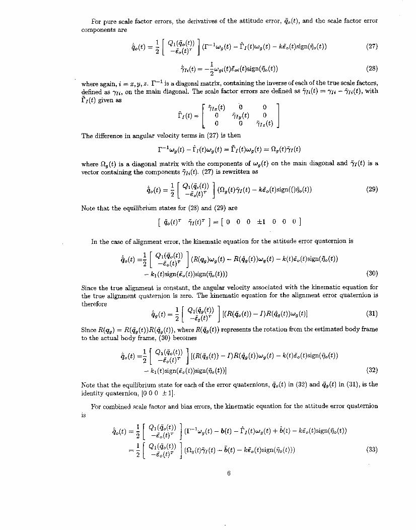
For pure scale factor errors, the derivatives of the attitude error, &(t), and the scale factor error components are

(28) 1 2 $1, (t) = - -wgi(t)Zoi (t)sign(ij, ( t ) )

where again, i = 2, y, z. I?-' is a diagonal matrix, containing the inverse of each of the true scale factors, defined as TIyli, on the main diagonal. The scale factor errors are defined as ;i.li(t) = ~ ~ y l i - + ~ ~ ( t ) , with l ; I ( t ) given as

The difference in angular velocity terms in (27) is then

r-L,(t) - t l(t)wg(t) = ~ ? ~ ( t ) ~ , ( t ) = o,(t);yl(t)

where R,(t) is a diagonal matrix with the components of wg(t ) on the main diagonal and q ~ ( t ) is a vector containing the components ;uli(t). (27) is rewritten as

Note that the equilibrium states for (28) and (29) are

[ @&)' ;ul(t)' 3 = [ 0 0 0 It1 0 0 0 ]

In the case of alignment error, the kinematic equation for the attitude error quaternion is

Since the true alignment is constant, the angular velocity associated with the kinematic equation for the true alignment quaternion is zero. The kinematic equation for the alignment error quaternion is therefore

Since R(q,) = R(qg(t))R(qg(t)), where R(ij,(t)) represents the rotation from the estimated body frame to the actual body frame, (30) becomes

- h (t)sign(Eo (t))sign(ii, (t))] (32)

Note that the equilibrium state for each of the error quaternions, cjo(t) in (32) and i jg(t) in (31), is the identity quaternion, [O 0 0 5 11.

For combined scale factor and bias errors, the kinematic equation for the attitude error quaternion is

6

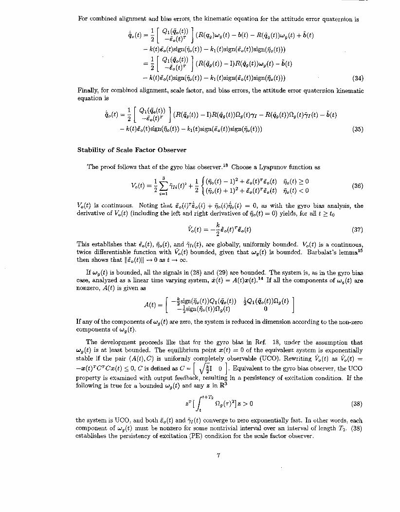
For combined alignment and bias errors, the kinematic equation for the attitude error quaternion is

Q1(4Jt)) (R(@,(t)) - I)R($(t))w,(t) - &(t) = 5 [ -E,(t)T ] - k(t)Eo( t)sign( 7-3, ( t ) ) - k l (t)sign(Eo(t))sign(7i, ( t ) ) ) (34)

Finally, for combined alignment, scale factor, and bias errors, the attitude error quaternion kinematic equation is

Stability of Scale Factor Observer

The proof follows that of the gyro bias observer.'* Choose a Lyapunov function as

( i i o ( t ) - + &(t)Tgo( t ) i j o ( t ) 2 0 (ijo(t) + 1)2 + &(t)'d,(t) ij,(t) < 0

3 1 Vo(t) = 2 C-iIi(t)2 t

i= 1

T 7 I*\ 1- __._ *: Y o ( & ) ~a ~ ~ I I L I I I U U U ~ . Notiiig that Eo(t jTZo(t j + ijo(tjijo(tj = 0, as with the gyro bias anaiysis, the derivative of Vo(t) (including the left and right derivatives of ijo(t) = 0) yields, for all t 2 to

(37) k 2

This establishes that d,( t ) , ij,(t), and y ~ i ( t ) , are globally, uniformly bounded. VJt) is a continuous, twice differentiable function with E(t) bounded, given that wg(t) is bounded. Barbalat's lemrnal5 then shows that IlZ,(t)ll 4 0 as t + m.

If wg(t ) is bounded, all the signals in (28) and (29) are bounded. The system is, as in the gyro bias case, analyzed as a linear time varying system, k( t ) = A(t)z(t).14 If all the components of wg(t) are nonzero, A(t) is given as

Vo(t) = --d,(t)TEl,(t)

If any of the components of wg( t ) are zero, the system is reduced in dimension according to the non-zero components of wg (t).

The development proceeds like that for the gyro bias in Ref. 18, under the assumption that wg(t ) is at least bounded. The equilibrium point z(t) = 0 of the equivalent system is exponentially stable if the pair ( A ( t ) , C ) is uniformly completely observable (UCO). Rewriting V o ( t ) as Vo(t) =

- - ~ ( t ) ~ C ~ C z ( t ) 5 0, C is defined as C = [ fi1 0 1. Equivalent to the gyro bias observer, the UCO property is examined with output feedback, resulting in a persistency of excitation condition. If the following is true for a bounded wg(t) and any z in W3

.T[J"'" R,(7)2]% > 0 t

the system is UCO, and both H o ( t ) and 'yr(t) converge to zero exponentially fast. In other words, each component of wg(t ) must be nonzero for some nontrivial interval over an interval of length Tz. (38) establishes the persistency of excitation (PE) condition for the scale factor observer.

7

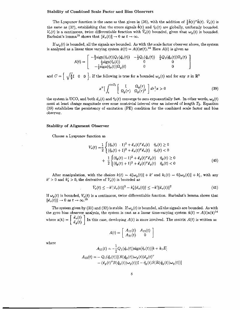
Stability of Combined Scale Factor and Bias Observers

The Lyapunov function is the same as that given in (36), with the addition of ;b( t )Tb(t) . Vo(t) is the same as (37), establishing that the errors signals b(t) and are globally, uniformly bounded. Vo(t) is a continuous, twice differentiable function with Vo(t) bounded, given that wg(t ) is bounded. Barbalat’s lemma1’ shows that IIZo(t)II -+ 0 as t -+ 00.

is analyzed as a linear time varying system k ( t ) = A(t)z(t).14 Here A(t) is given as If wg(t ) is bounded, all the signals are bounded. As with the scale factor observer above, the system

I [ -$sign(% ( W g ( t ) 0 0

- $ ~ i d % ( t ) ) Q i (&(t)) -4Qi ( G o ( t ) > 4Qi ( d o ( t ) ) % ( t ) 4 sign(?jo(t)) 0 0 A(t) =

and C = [ 41 0 0 1. If the following is true for a bounded w g ( t ) and for any 2: in W3

the system is UCO, and both Eo( t ) and q I ( t ) converge to zero exponentially fast. In other words, wg(t) must at least change magnitude over some nontrivial interval over an interval of length T2. Equation (39) establishes the persistency of excitation (PE) condition for the combined scale factor and bias observer.

Stability of Alignment Observer

Choose a Lyapunov function as

After manipulation, with the choices k(t) = 411ug(t)ll + IC’ and ICl(t) = 611wg(t)ll + I C : , with any k‘ > 0 and IC: > 0, the derivative of Vo(t) is bounded as

%(t) 5 -k’ll&(t)1I2 - k;(Ido(t)lJ I -k’ll~o(t)ll2 (41)

If wg(t) is bounded, Vo(t) is a continuous, twice differentiable function. Barbalat’s lemma shows that IlCO(t)II -+ 0 as t ---t 00.15

The system given by (31) and (32) is stable. If w,(t) is bounded, all the signals are bounded. As with the gyro bias observer analysis, the system is cast as a linear time-varying system x(t) = A(t)x(t)14

where x( t ) = [ ‘!%’ti; ] In this case, developing A(t) is more involved. The matrix A(t) is written as

where

8

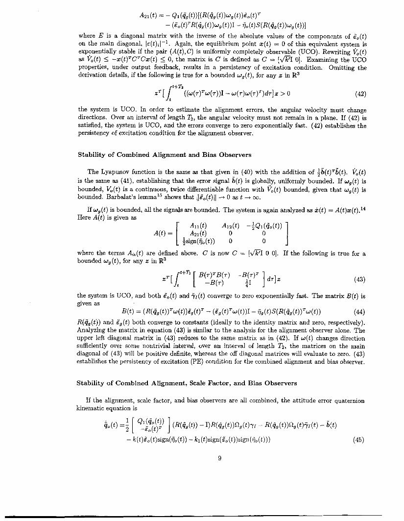
A21 ( t ) = - &I ( G g ( t ) ) [ ( W G g (t>)Wg ( t ) )Eo ( t ) '

- (Eo(t)TR(qgS(t))W9(t))I - 7jo(t)S(R(qg(t))wg(t))l where E is a diagonal matrix with the inverse of the absolute values of the components of E,(t) on the main diagonal, J ~ ( t ) ~ l - l . Again, the equilibrium point z(t) = 0 of this equivalent system is exponentially stable if the pair (A(t), C) is uniformly completely observable (UCO). Rewriting Vo(t) as Vo(t) I -s(t)'C'Cz(t) 5 0, the matrix is C is defined as C = [&I 01. Examining the UCO properties, under output feedback, results in a persistency of excitation condition. Omitting the derivation details, if the following is true for a bounded wg( t ) , for any z in R3

the system is UCO. In order to estimate the alignment errors, the angular velocity must change directions. Over an interval of length T2, the angular velocity must not remain in a plane. If (42) is satisfied, the system is UCO, and the errors converge to zero exponentially fast. (42) establishes the persistency of excitation condition for the alignment observer.

Stability of Combined Alignment and Bias Observers

The Lyapunov function is the same as that given in (40) with the addition of +b(t)'b(t). Vo(t) is the same as (41), establishing that the error signal b(t) is globally, uniformly bounded. If u g ( t ) is bounded, Vo(t) is a continuous, twice differentiable function with Vo(t) bounded, given that wg(t ) is bounded. Barbalat's lemma15 shows that IIEo(t)II + 0 as t + 00.

If w,(t) is bounded, all the signals are bounded. The system is again analyzed as k( t ) = A(t)z( t ) .14 Here A(t) is given as

1 [ 3sign(q0(t)) 0 0

Aii ( t ) A12(t) -;Qi(&(t)) A(t) = A2l(t) 0 0

where the terms Ai,(t) are defined above. C is now C = [nI 0 01. If the following is true for a bounded wg( t ) , for any z in R3

the system is UCO, and both E,(t) and ;i.l(t) converge to zero exponentially fast. The matrix B(t) is given as

R(Gg(t)) and Zg(t) both converge to constants (ideally to the identity matrix and zero, respectively). Analyzing the matrix in equation (43) is similar to the analysis for the alignment observer alone. The upper left diagonal matrix in (43) reduces to the same matrix as in (42). If w ( t ) changes direction sufficiently over some nontrivial interval, over an interval of length T2, the matrices on the main diagonal of (43) will be positive definite, whereas the off diagonal matrices will evaluate to zero. (43) establishes the persistency of excitation (PE) condition for the combined alignment and bias observer.

a t ) = (R(~gb(t>>'w(t)>~g(t)' - (Eg(t)TW(t))I - 7 j~( t>s (R(~g( t> )=W( t ) ) (44)

Stability of Combined Alignment, Scale Factor, and Bias Observers

If the alignment, scale factor, and bias observers are all combined, the attitude error quaternion kinematic equation is

9

The Lyapunov function is the same as the alignment observer with +b(t)’b(t) and + T I ( t ) T q I ( t ) added. Vo(t) is also the same as for the alignment observer, with the addition of the term 71. If an a priori upper bound is known for 7 1 , Vo(t) is bounded as in (41). This establishes that b(t) and ? I ( t ) are bounded. If wg(t) is bounded, Vo(t) is a continuous, twice differentiable function with Vo(t) bounded, given that wg(t ) is bounded. Barbalat’s lemma15 shows that IIE,(t)II -+ 0 as t -+ 00.

If wg(t ) is bounded, all the signals are bounded. The system is again analyzed as k ( t ) = A(t)z(t).14 Here A(t) is given as

All (t) AL(t) -;SI (Go( t ) )R(@g ( t ) ) O g ( t ) -4Q1 (&(t)j A21 ( t ) 0 0

- $29 (t>R(@g(t)>’sign(rio(t)) 0 0 0 + sign(ij0 ( t ) 0 0 0

A(t) =

where All(t) and A21(t) are defined for the alignment observer. Ai2(t) is similar to A12(t) with R(@g(t))ilg(t)7~ replacing R($(t))w,(t). C is now C = [*I 0 0 01. Equivalently to the alignment observer, the UCO property is examined with output feedback, resulting in a persistency of excitation condition. If the following is true for a bounded wg(t) , for any z in W3 (the time argument is omitted for clarity)

(46)

where

1 - ;R(qg)~(W-f l , 11 4 J

BTB

and here

B(t ) = ( R ( Q 9 ) R ( ~ 9 ( t ) ) T ~ 2 , ( t ) ~ r ) ~ 9 ( t > T - (~g( t )TR(qg)R(~9( t ) )To9( t )YI ) I - 75, (t>s(R(4,)R(~9(t))’s2, ( t )7r)

Again, R(ijg(t)) and E g ( t ) converge to constants. If the angular velocity, in addition to being bounded, satisfies the integral in equation (46) over an interval of length T2, the system UCO, and the errors &(t), ;i.~(t), and E g ( t ) converge to zero exponentially fast.

CLOSED LOOP STABILITY

The nonlinear tracking control strategy proposed in Ref. 19 and summarized above cannot be implemented because exact measurements of the angular velocity w( t ) are not available. Instead, a certainty equivalence approach is proposed using estimates w ( t ) generated by the observer equations, resulting in

where 2 ( t ) = G(t ) - w,(t), &(t) = G(t) - R ( & ( t ) ) ~ d ( t ) , and

U ( t ) = -KDS(t) + H&,(t) - S(HG(t))w,( t ) (47)

& ( t ) = R( &( t ) ) b d (t) - s( 5, (t))R( GC (t))wd ( t ) - A Q i (& ( t ) ) & c (t > Substitution of (47) into (12), the attitude dynamics, results in the following closed loop equation18

HS( t ) - S(Hw(t))s( t ) + K,s(t) = A ( g c ( t ) , W d ( t ) ) i ( t ) (48)

where A( Gc ( t ) Wd ( t ) ) = -S(W, ( t ) )H-HS(R( Gc ( t ) ) W d ( t ) ) + XHQl ( G c ( t ) ) +KD = A’( Gc ( t ) w d ( t ) ) +KD. A’(&(t),wd(t)) is a bounded matrix over any solution of the coupled dynamics (19) or (22), (20) or (21) or (23), (12), and (47).

10

In the case of gyro bias, the error term s(t) is written as

i ( t ) = w ( t ) - &(t) = -b( t )

Hi(t) - S("J(t))s(t) + K ~ s ( t ) = -A(ic(t) , W d ( t ) ) b ( t )

The closed loop dynamics are then written as

(49)

The control law (47) results in global stability and asymptotically perfect tracking, IIE,(t)JI 4 0, IIGc(t)ll -+ 0. The proof is given in detail in Ref. 18.

Closed Loop Stability with Constant Scale Factor Error

Given the Lyapunov function V'(t) = s ( t )THs( t ) , the derivative of Vc(t), using (48), is

K(t) = - ~ ( t ) ~ K D s ( t ) + s(t)'A(&(t), ~ ( t ) ) ( ~ ( t ) - i ( t ) ) (50)

Rewriting the error term

s(t) - q t ) = ~ ( t ) - ;(ti = r--Lg(t) - f I ( t )wg( t ) = r-Lg(t) - F1(t)wg(t) = F1(t)wg(t)

Since wg( t ) = I'w(t) = r(s(t) + ur(t)) equation 51 is rewritten as

The convergence of s( t ) to zero depends on the exponential convergence of the scale factor errors, which in turn depends on the angular velocity ug(t) generated by the applied control. The derivative of V,(t) is bounded as

where k, is the smallest eigenvalue of K,,

If the scale factors are known to be bounded within a positive region, with projection implemented in the observer such that the scale factor estimates remain with a bounded, positive region,20 and k, is sufficiently large, the closed loop system is uniformly, ultimately bounded. If the angular velocity, wg(t) , in addition to being bounded (which ensures that the observer error terms are at least bounded), satisfies (38), the system is UCO and the scale factor errors converge to zero exponentially fast. In this case Theorem B.8 of Ref. 15 applies. Vc(t) converges to zero exponentially fast, which means s( t ) converges to zero exponentially fast, for any kg > 0 and without placing restrictions on the scale factors and the scale factor estimates. With the convergence of s( t ) 4 0, the proof of convergence of the actual attitude and rate errors follows exactly as in the gyro bias analysis of Ref. 18. The end result of which is limt-toollEc(t)ll = 0 and limt4,11Gc(t)ll = 0.

Closed Loop Stability wi th Constant Scale Factor and Bias Errors

The Lyapunov function is the same as that above, with &it) given by (50). The error term is now

11

Since wg( t ) = I ' (w(t) + b) (54) is

s(t) - q t ) = FI(t)r(s(t) + U T @ ) + b) - b(t)

Finally, Vc(t) is bounded as

%(t) 5 - k D l l s ( t ) 1 1 2 + (kD + C ' ) ~ * I ( t ) m r l l s ( t ) 1 1 2 + ( k D f ~ ' ) ~ * ~ ~ ~ w ~ ( t ) ~ ~ ~ ~ s ( t ) ~ ~ ~ ~ ~ ( t )

+ ( k D + C ' ) m r l l b l l l l S ( t ) l l ~ ~ r ( t > + ( k D + c'>lls(t>llll'(t>ll (55)

where k,, C', and wT(t ) are defined above. Again, if the scale factors are known to be bounded within a positive region, with projection implemented in the observer such that the scale factor estimates remain within a bounded, positive region,20 and kD is sufficiently large, the closed loop system is uniformly, ultimately bounded. If the angular velocity, wg(t) , in addition to being bounded (which ensures that the observer error terms are at least bounded), satisfies (39), the system is UCO and the scale factor and bias errors converge to zero exponentially fast. As detailed above, the error B ( t ) converges to zero, resulting in convergence of the attitude and rate tracking errors.

Closed Loop Stability with Constant Alignment Error

Again, using the Lyapunov function Vc(t) = i s ( t )THs( t ) , the derivative of Vc(t) is

v c ( t ) = -s(t)TKDS(t) + s(t)'A(@C(t), W d ( t ) ) i ( t )

Thc C E G r tcrm q t ) is rcwrittc:: 2s

s( t ) - i ( t ) = w(t ) - Lj( t ) = w(t ) - R(&(t))wg(t) = (I - R(@,(t))=)u(t)

Substituting w ( t ) = s(t) + o,(t) from (16), S ( t ) is

The convergence of s ( t ) to zero depends on the exponential convergence of the alignment errors, which in turn depends on the angular velocity w ( t ) generated by the applied control. The derivative of Vc(t) is bounded as

If the alignment error is less than 90 degrees and k D is sufficiently large, the closed loop system is uniformly, ultimately bounded. If the angular velocity, w( t ) , in addition to being bounded, satisfies (42), the system is UCO and the alignment errors, E g ( t ) , converge to zero exponentially fast. As in the case of scale factor error, Theorem B.8 of Ref.15 applies. Vc(t) converges to zero exponentially fast, which means s ( t ) converges to zero exponentially fast, for any kg > 0 and any alignment error. With the convergence of s ( t ) + 0, the proof of convergence of the actual attitude and rate errors follows exactly as in the gyro bias analysis of Ref. 18, l i m ~ . + m ~ ~ 2 c ( t ) ~ ~ = 0 and l imt -+m~~Gc( t )~ / = 0.

Closed Loop Stability with Constant Alignment and Bias Errors

12

The angular velocity, wg(t) , is written as

The convergence of s( t ) to zero depends on the exponential convergence of the alignment errors, which in turn depends on the angular velocity w(t) generated by the applied control. The derivative of V'(t) can be bounded, again, after some manipulation, as

R(t> 5 - kDlls(t)112 f 2(kD -k C ' ) l l ~ g s ( t ) l ( l l s ( t ) 1 1 2

f 2 ( k D + C')(llwr(t) 11 I l s ( t > l l l lEg(t) l l + l l b l l I l s ( t ) / l l lEg( t ) 1 1 ) + (b + C') IKt) II II b(t) II (59)

where k D and C' are defined above. If the alignment error angle is less than 90 degrees and kD is sufficiently large, the closed loop system is uniformly, ultimately bounded. If the angular velocity, w(t) , in addition to being bounded, satisfies (43), the system is UCO and the alignment and bias errors, E g ( t ) , converge to zero exponentially fast. Again, this ensures that s( t ) converges to zero, for any k D > 0 and any alignment error. With the convergence of s( t ) + 0, the proof of convergence of the actual attitude and rate errors is the same as above. The end result of which is limt+m~~Ec(t)l~ = 0 and limt+m llGc(t) 1 1 = 0.

OBSERVER SIMULATION RESULTS

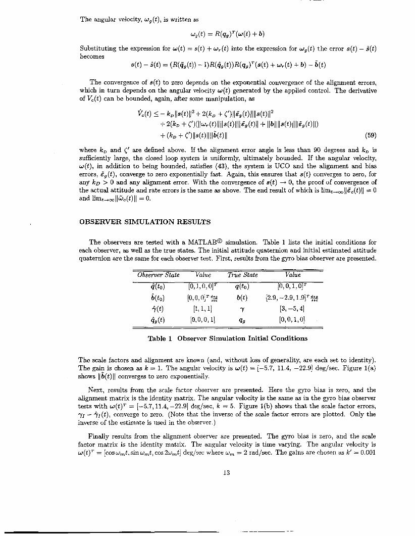
The observers are tested with a MATLAB@ simulation. Table 1 lists the initial conditions for each observer, as well as the true states. The initial attitude quaternion and initial estimated attitude quaternion are the same for each observer test. First, results from the gyro bias observer are presented.

Observer State Value True State Value

b ( t 0 ) [O, 170, 01' 4 t o ) [O,O, 1, 01'

@o) [O, 0, 01' 2 b(t) [2.9, -2.9, 1.91'2

W ) [I, 1,11 7 [3, -5,4] 4l (t) [O,O,O, 11 49 [ O , O , l , O l

Table 1 Observer Simulation Initial Conditions

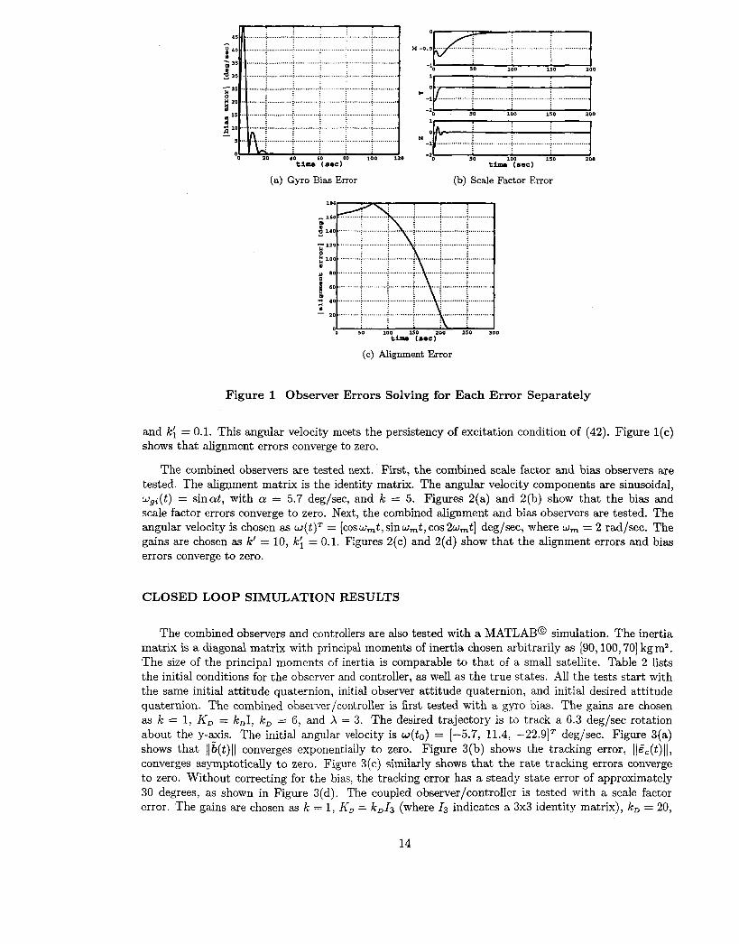
The scale factors and alignment are known (and, without loss of generality, are each se to identity). The gain is chosen as k = 1. The angular velocity is w( t ) = [-5.7, 11.4, -22.91 deg/sec. Figure l(a) shows IIb(t) 11 converges to zero exponentially.

Next, results from the scale factor observer are presented. Here the gyro bias is zero, and the alignment matrix is the identity matrix. The angular velocity is the same as in the gyro bias observer tests with w(t)' = [-5.7,11.4, -22.91 deg/sec, k = 5. Figure l(b) shows that the scale factor errors, 7 1 - qr(t), converge to zero. (Note that the inverse of the scale factor errors are plotted. Only the inverse of the estimate is used in the .observer.)

Finally results from the-alignment observer are presented. The gyro bias is zero, and the scale factor matrix is the identity matrix. The angular velocity is time varying. The angular velocity is w(t)' = [coswmt, sinw,t, cos2w,t] deg/sec where w, = 2 rad/sec. The gains are chosen as k' = 0.001

time (sac)

(a) Gyro Bias Error

............... ~ ................... j ........................

I 50 100 150 100

................... : ....................... i ..................... i ...................... * I 4 100 1so 200

-1 ............................................................................................. -2 so 100 150 20.

t h u (sac)

(b) Scale Factor Error

Oo so 100 150 aoo 150 300 ti- (8.C)

(c) Alignment Error

Figure 1 Observer Errors Solving for Each Error Separately

and ki = 0.1. This angular velocity meets the persistency of excitation condition of (42). Figure l(c) shows that alignment errors converge to zero.

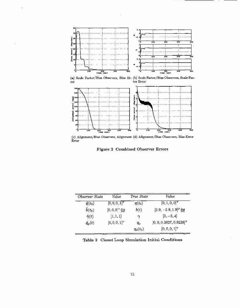
The combined observers are tested next. First, the combined scale factor and bias observers are tested. The aligpment matrix is the identity matrix. The angular velocity components are sinusoidal, ugi(t) = sinat, with a = 5.7 deg/sec, and k = 5. Figures 2(a) and 2(b) show that the bias and scale factor errors converge to zero. Next, the combined alignment and bias observers are tested. The angular velocity is chosen as w(t)' = (cos umtr sin u,t, cos 2w,t] deg/sec, where w, = 2 rad/sec. The gains are chosen as k' = 10, = 0.1. Figures 2(c) and 2(d) show that the alignment errors and bias errors converge to zero.

CLOSED LOOP SIMULATION RESULTS

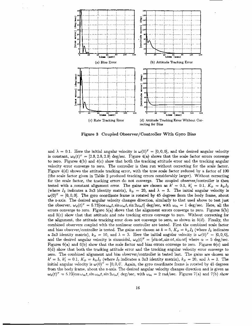
The combined observers and controllers are also tested with a MATLAB@ simulation. The inertia matrix is a diagonal matrix with principal moments of inertia chosen arbitrarily as [go, 100,70] kg mz. The size of the principal moments of inertia is comparable to that of a small satellite. Table 2 lists the initial conditions for the observer and controller, as well as the true states. All the tests start with the same initial attitude quaternion, initial observer attitude quaternion, and initial desired attitude quaternion. The combined observer/controller is first tested with a gyro bias. The gains are chosen as k = 1, KD = k,I, kD = 6, and X = 3. The desired trajectory is to track a 6.3 deg/sec rotation about the y-axis. The initial angular velocity is w(t0) = [-5.7, 11.4, -22.9IT deg/sec. Figure 3(a) shows that Il&(t)lJ converges exponentially to zero. Figure 3(b) shows the tracking error, IIEc(t)ll, converges asymptotically to zero. Figure 3(c) similarly shows that the rate tracking errors converge to zero. Without correcting for the bias, the tracking error has a steady state error of approximately 30 degrees, as shown in Figure 3(d). The coupled observer/controller is tested with a scale factor error. The gains are chosen as k = 1, KD = kD13 (where I3 indicates a 3x3 identity matrix), k, = 20,

14

0.5, I

....... -0.5 .................. . . . j . . . . . . . . . . L ...... ............:.. ..................

0 I 4

-1

...... )I -1 ...................... i ................... .1... ................... i .......................

........

200 300 400 t h I.-)

100

(a) Scale Factor/Bias Observers, Bias Er- (b) Scale Factor/Bias Observers, Scale Fac- ror tor Error

20 ................ j .............. i . . . . . . _ . . . ; ................

00 1;o 2;o ,A0 . io 500 t h (..0)

(c ) Alignment/Bias Observers, Alignment (d) Alignment/Bias Observers, Bias Error Error

Figure 2 Combined Observer Errors

Table 2 Closed Loop Simulation Initial Conditions

15

(a) Bias Error (b) Attitude Tracking Error

o ao bo so 10 xoo i ao tins ( S O C )

(c) Rate Tracking Error

............... ............... ............... ............... ............... .......... 110 ~

160 i j 2 i .i...

0 140 ............... i ............................................................. 0

............... I II

20 ............... i ............... j ............... 6 ............... i ............... i ..............

‘0 i o i o A i o 100 i a o t h (smc)

(d) Attitude Tracking Error Without Cor- recting for Bias

Figure 3 Coupled Observer/Controller With Gyro Bias

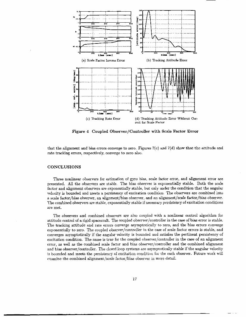
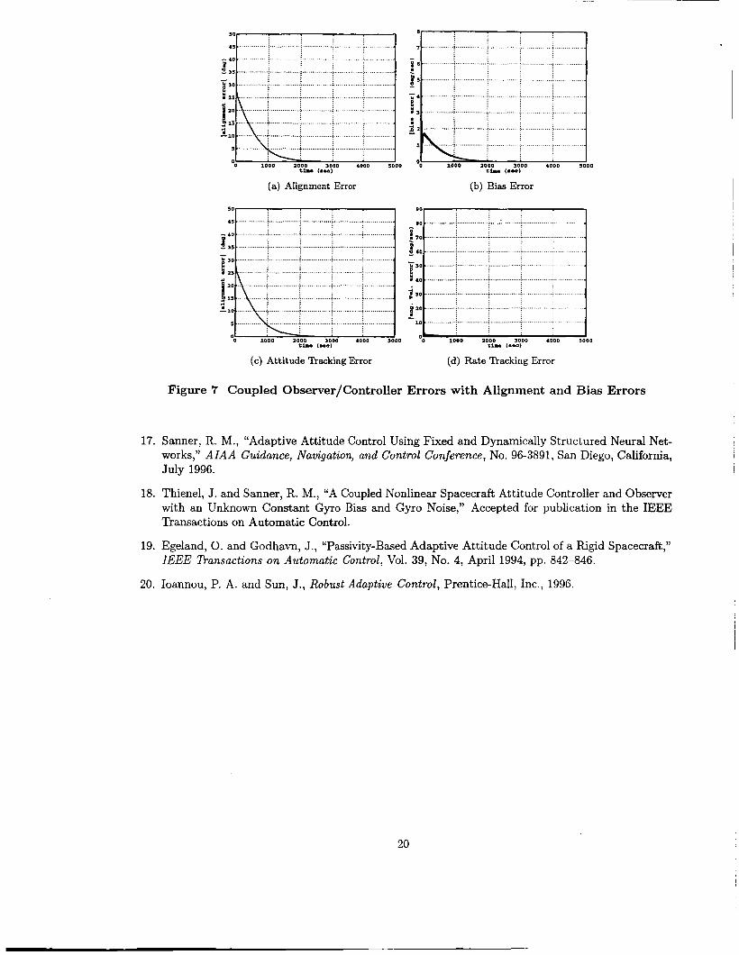
and X = 0.1. Here the initial angular velocity is ~ ( 0 ) ~ = [O,O,O], and the desired angular velocity is constant, u d ( t ) = = [2.8,2.8,2.8] deg/sec. Figure 4(a) shows that the scale factor errors converge to zero. Figures 4(b) and 4(c) show that both the tracking attitude error and the tracking angular velocity error converge to zero. The controller is then run without correcting for the scale factor. Figure 4(d) shows the attitude tracking error, with the true scale factor reduced by a factor of 100 (the scale factor given in Table 2 produced tracking errors considerably larger). Without correcting for the scale factor, the tracking errors do not converge. The coupled observer/controller is then tested with a .constant alignment error. The gains are chosen as k’ = 0.1, ki = 0.1, KD = k,I3 (where I3 indicates a 3x3 identity matrix), kD = 20, and X = 3. The initial angular velocity is ~ ( 0 ) ~ = [0, O,O]. The gyro coordinate frame is rotated by 45 degrees from the body frame, about the z-axis. The desired angular velocity changes direction, similarly to that used above to test just the observer, U d ( t ) T = 5.73[cosw,t,sinw,t,sin2wmt] deg/sec, with w, = 1 deg/sec. Here, all the errors converge to zero. Figure 5(a) shows that the alignment errors converge to zero. Figures 5(b) and 5(c) show that that attitude and rate tracking errors converge to zero. Without correcting for the alignment, the attitude tracking error does not converge to zero, as shown in 5(d). Finally, the combined observers coupled with the nonlinear controller are tested. First the combined scale factor and bias observer/controller is tested. The gains are chosen as k = 5 , KD = k ~ I 3 (where 13 indicates a 3x3 identity matrix), k , = 10, and X = 3. Here the initial angular velocity is ~ ( 0 ) ~ = [O,O,O] , and the desired angular velocity is sinusoidal, Wd( t )= = [sin at, sin at, sin at] where a = 5 deg/sec. Figures 6(a) and 6(b) show that the scale factor and bias errors converge to zero. Figures 6(c) and 6(d) show that both the tracking attitude error and the tracking angular velocity error converge to zero. The combined alignment and bias observer/controller is tested last. The gains are chosen as k’ = 5, ki = 0.1, KD = kD13 (where 13 indicates a 3x3 identity matrix), k , = 20, and X = 3. The initial angular velocity is ~ ( 0 ) ~ = [O,O,O]. Again, the gyro coordinate frame is rotated by 45 degrees from the body frame, about the z-axis. The desired angular velocity changes direction and is given as W d ( t ) T = 5.73[cosw,t,sinw,t,sin2w,t] deg/sec, with w, = 2 rad/sec. Figures 7(a) and 7(b) show

16

(a) Scale Factor Inverse Error (b) Tracking Attitude Error

(c) Tracking Rate Error (d) Tracking Attitude Error Without Cor- rect for Scale Factor

Figure 4 Coupled Observer/Controller with Scale Factor Error

that the alignment and bias errors converge to zero. Figures 7(c) and 7(d) show that the attitude and rate tracking errors, respectively, converge to zero also.

CONCLUSIONS

Three nonlinear observers for estimation of gyro bias, scale factor error, and alignment error are presented. All the observers are stable. The bias observer is exponentially stable. Both the scale factor and alignment observers are exponentially stable, but only under the condition that the angular velocity is bounded and meets a persistency of excitation condition. The observers are combined into a scale factor/bias observer, an alignment/bias observer, and an alignment/scale factor/bias observer. The combined observers are stable, exponentially stable if necessary persistency of excitation conditions are met.

The observers and combined observers are also coupled with a nonlinear control algorithm for attitude control of a rigid spacecraft. The coupled observer/controller in the case of bias error is stable. The tracking attitude and rate errors converge asymptotically to zero, and the bias errors converge exponentially to zero. The coupled observer/controller in the case of scale factor errors is stable, and converges asymptotically if the angular velocity is bounded and satisfies the pertinent persistency of excitation condition. The same is true for the coupled observer/controller in the case of an alignment error, as well as the combined scale factor and bias observer/controller and the combined alignment and bias observer/controller. The closed loop systems are asymptotically stable if the angular velocity is bounded and meets the persistency of excitation conditiori for the each observer. Future work will examine the combined alignment/scale factor/bias observer in more detail.

17

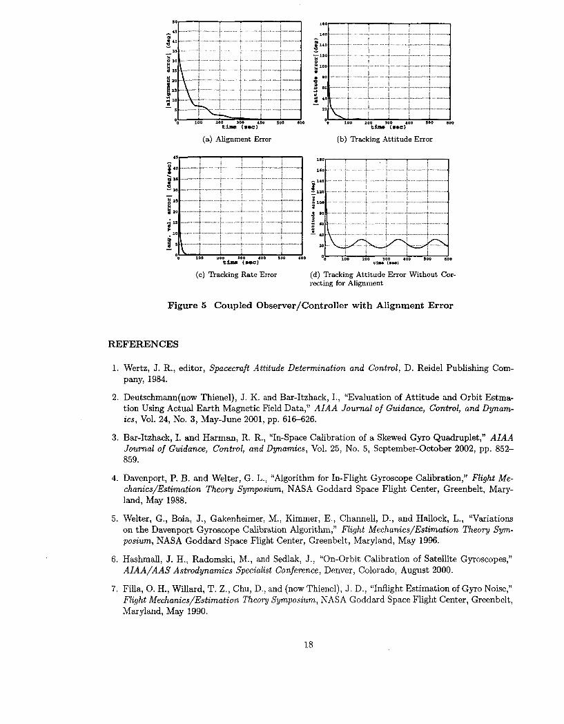
(a) Alignment Error (b) Tracking Attitude Error

t h o (..=I

(c) Tracking Rate Error (d) Tracking Attitude Error Without Cor- recting for Alignment

Figure 5 Coupled Observer/Controller wi th Alignment Error

REFERENCES

1. Wertz, J. R., editor, Spacecraft Attitude Determination and Control, D. Reidel Publishing Com- pany, 1984.

2. Deutschmann(now Thienel), J. K. and Bar-Itzhack, I., “Evaluation of Attitude and Orbit Estma- tion Using Actual Earth Magnetic Field Data,” AIAA Journal of Guidance, Control, and Dynam- ics, Vol. 24, No. 3, May-June 2001, pp. 616-626.

3. Bar-Itzhack, I. and Harman, R. R., “In-Space Calibration of a Skewed Gyro Quadruplet,” AIAA Journal of Guidance, Control, and Dynamics, Vol. 25, No. 5, September-October 2002, pp. 852- 859.

4. Davenport, P. B. and Welter, G. L., “Algorithm for In-Flight Gyroscope Calibration,” Flight Me- chanics/Estimation Theory Symposium, NASA Goddard Space Flight Center, Greenbelt, Mary- land, May 1988.

5 . Welter, G., Boia, J., Gakenheimer, M., Kimmer, E., Channell, D., and Hallock, L., “Variations on the Davenport Gyroscope Calibration Algorithm,” Flight Mechanics/Estimation Theoy Sym- posium, NASA Goddard Space Flight Center, Greenbelt, Maryland, May 1996.

6. Hashmall, J. H., Radomski, M., and Sedlak, J., “On-Orbit Calibration of Satellite Gyroscopes,” AIAA/AAS Astrodynamics Specialist Conference , Denver, Colorado, August 2000.

7. Filla, 0. H., Willard, T. Z., Chu, D., and (now Thienel), J. D., “Inflight Estimation of Gyro Noise,” Flight Mechanics/Estimation Theoy Symposium, NASA Goddard Space Flight Center, Greenbelt, Maryland, May 1990.

18

35 - . . . . . . . . . . . . ..: .............. : ................ I -0.5 . . . . . . . E

: -lo .. ~ .......... ~ ................ - ” : 1 5 . . . . . . . . . . . . . . . . . . . ~ ............... I .................. i ...................

loo 4oo 600 BOO IOOO 8 lo . . . . ;. . . . .j . . . . . . . ..I ............. ................... - I 4

15 . . . . . . . . . . . . ;. . . ..........I.... ............ i ...................

0 :lo... . . . . . . . . . . . i ... . . . . . . . . b .............. i .................. .

.:. ............... 2 .................. : ................... z

400 Si0 &O

180 160 1 I

1000

................. .............. ................. .................. ..................

............. ........ . . . . . . ............... ...........

i :

.............. . . . . . . . . . . . ................................. )... ; 5 i......

;.. ~ ....E

- 6 0 . ... . . . . . . : ................. : .................. ........ ......... ............. .................

.......... . . . . . . ............. ..................

j :.. i.

; ; i

0 100 I 0 0 600 800 1000 t i r (..a1

1;O Si0 Si0 1000 tiu l..ol

(c) Attitude Tracking Error (d) Rate Wacking Error

Figure 6 Coupled Observer/Controller Errors with Scale Factor and Bias Errors

8. Sedlak, J., Hashmall, J. H., and Airapetian, V., “Comparison of On-Orbit Performance of Rate Sensing Gyroscopes,” International Symposium on Spaceflight Dynamics, Biarritz, F’rance, June 2000.

9. Alonso, R., Crassidis, J. L., and Junkins, J. L., “Vision-Based Relative Navigation for Formation Flying of Spacecraft,” A I A A Guidance, Navigation, and Control Conference, No. AIAA-2000-4439, Denver, Colorado, August 2000.

10. Salcudean, S., “A Globally Convergent Angular Velocity Observer for Rigid Body Motion,” IEEE Transactions on Automatic Control, Vol. 36, No. 12, December 1991, pp. 1493-1496.

11. Vik, B., Shiriaev, A., and Fossen, T. I., “Nonlinear Observer Design for Integration of DGPS and INS,” New Directions in Nonlinear Observer Design, Springer-Verlag, 1999.

12. Bokkovik, J. D., Li, S.-M., and Mehra, R. K., “A Globally Stable Scheme for Spacecraft Control in the Presence of Sensor Bias,” 2000 IEEE Aerospace Conference, Big Sky, Montana, March 2000.

13. BoSkovik, J. D., Li, S.-M., and Mehra, R. K., “Fault Tolerant Control of Spacecraft in the Presence of Sensor Bias,” American Control Conference, Chicago, Illinois, March 2000.

14. Khalil, H. K., Nonlinear Systems, Prentice-Hall, Inc., 2nd ed., 1996.

15. Krsti6, M., Kanellakopoulos, I., and Kokotovic, P., Nonlinear and Adaptive Control Design, John Wiley and Sons, Inc., 1995.

16. Shuster, M. D., “A Survey of Attitude Representations:” The Journal of Astronautical Sciences, Vol. 41, No. 4, October-December 1993, pp. 439-517.

19

50

45 - 40

a 35

“ 30 ............................. : .............. .: ......................... ............. ..; . . . . . .;.,. .........

- e

.............. .........................

................. i ............ i.,. .........

................. i .................. ; ...................

................. + ............. .P... .............

................. i .................. i ...........................

................ ; ................. ; ........ :. . . . .

* s o ................... ...................................... i ........ 4 . . . - ........ .......... f ,Q ................................................. ..:..

ij 20 ................ i. ............... L.. ......... ..i . . . . . . . . . . .

........ ; .................. i ................. I.. .....................

10 ................. j.. .......... ....+.................. *. . . . . . . ~ . . . - !

(a) Alignment Error (b) Bias Error

90

,Q .................. ) ...((..........,............................ .................. . . . ............... .................. .................. .................. 50

45 . . . . . . . . . . . . . . . . . . . . . . ; + < -

o iooo aooo 3000 4000 5000 t h (..el

(c) Attitude Tracking Error (d) Rate Tracking Error

Figure 7 Coupled Observer/Controller Errors with Alignment and Bias Errors

17. Sanner, R. M., “Adaptive Attitude Control Using Fixed and Dynamically Structured Neural Net- works,” AIAA Guidance, Navigation, and Control Conference, No. 96-3891, San Diego, California, July 1996.

18. Thienel, J. and Sanner, R. M., “A Coupled Nonlinear Spacecraft Attitude Controller and Observer with an Unknown Constant Gyro Bias and Gyro Noise,” Accepted for publication in the IEEE Transactions on Automatic Control.

19. Egeland, 0. and Godhavn, J., “Passivity-Based Adaptive Attitude Control of a Rigid Spacecraft,” IEEE Transactions o n Automatic Control, Vol. 39, No. 4, April 1994, pp. 842-846.

20. Ioannou, P. A. and Sun, J., Robust Adaptive Control, Prentice-Hall, Inc., 1996.

20