1Scientific Data | (2020) 7:92 | https://doi.org/10.1038/s41597-020-0427-5

www.nature.com/scientificdata

Gut microbiome diversity detected by high-coverage 16S and shotgun sequencing of paired stool and colon sampleJoan Mas-Lloret 1,2,3, Mireia Obón-Santacana1,2,3, Gemma Ibáñez-Sanz 1,2,3,4, Elisabet Guinó1,2,3, Miguel L. Pato 5, Francisco Rodriguez-Moranta4, Alfredo Mata6, Ana García-Rodríguez7, Victor Moreno 1,2,3,8 ✉ & Ville Nikolai Pimenoff1,2,3,9 ✉

The gut microbiome has a fundamental role in human health and disease. However, studying the complex structure and function of the gut microbiome using next generation sequencing is challenging and prone to reproducibility problems. Here, we obtained cross-sectional colon biopsies and faecal samples from nine participants in our COLSCREEN study and sequenced them in high coverage using Illumina pair-end shotgun (for faecal samples) and IonTorrent 16S (for paired feces and colon biopsies) technologies. The metagenomes consisted of between 47 and 92 million reads per sample and the targeted sequencing covered more than 300 k reads per sample across seven hypervariable regions of the 16S gene. Our data is freely available and coupled with code for the presented metagenomic analysis using up-to-date bioinformatics algorithms. These results will add up to the informed insights into designing comprehensive microbiome analysis and also provide data for further testing for unambiguous gut microbiome analysis.

Background & SummaryThe gut microbiome is highly dynamic and variable between individuals, and is continuously influenced by fac-tors such as individual’s diet and lifestyle1,2, as well as host genetics3. Next generation sequencing (NGS) has greatly enhanced our understanding of the human microbiome, as these techniques allow researchers to investi-gate variation in diversity and abundance of bacteria in a culture-independent manner. Recent developments in bioinformatics have permitted the identification of thousands of novel bacterial and archaeal species and strains identified in human and non-human environments through metagenome assembly4–6. For colorectal cancer (CRC), recent large-scale studies have revealed specific faecal microbial signatures associated with malignant gut transformations, although the causal role of gut bacterial ecosystem in CRC development is still unclear7,8.

The 16S small subunit ribosomal gene is highly conserved between bacteria and archaea, and thus has been extensively used as a marker gene to estimate microbial phylogenies9. The 16S rRNA gene contains nine hyper-variable regions (V1-V9) with bacterial species-specific variations that are flanked by conserved regions. Hence, the amplification of 16S rRNA hypervariable regions can be used to detect microbial communities in a sample typically down to the genus level10, and species-level assignments are also possible if full-length 16S sequences are retrieved11.

1Oncology Data Analytics Program, catalan institute of Oncology (icO), Barcelona, Spain. 2colorectal cancer Group, OncOBeLL Program, Bellvitge institute of Biomedical Research (iDiBeLL), Barcelona, Spain. 3consortium for Biomedical Research in epidemiology and Public Health (ciBeReSP), Barcelona, Spain. 4Gastroenterology Department, Bellvitge University Hospital-IDIBELL, Hospitalet de Llobregat, Barcelona, Spain. 5cancer epigenetics and Biology Program (PeBc), Bellvitge Biomedical Biomedical Research institute (iDiBeLL), Barcelona, catalonia, Spain. 6Digestive System Service, Moisés Broggi Hospital, Sant Joan Despí, Spain. 7endoscopy Unit, Digestive System Service, Viladecans Hospital-IDIBELL, Viladecans, Spain. 8Department of clinical Sciences, faculty of Medicine, University of Barcelona, Barcelona, Spain. 9National Cancer Center Finland (FICAN-MID) and Karolinska Institute, Stockholm, Sweden. ✉e-mail: v.moreno@iconcologia.net; ville.pimenoff@ki.se

DATA DESCRIpTOR

OpEN

2Scientific Data | (2020) 7:92 | https://doi.org/10.1038/s41597-020-0427-5

www.nature.com/scientificdatawww.nature.com/scientificdata/

However, conserved regions are not entirely identical across groups of bacteria and archaea, which can have an effect on the PCR amplification step. Notably, among the conserved regions of the 16S gene, central regions are more conserved, suggesting that they are less susceptible to producing bias in PCR amplification12. Furthermore, an in silico study has shown that the V4-V6 regions perform better at reproducing the full taxonomic distribution of the 16S gene13. In another study, a constructed mock sample was sequenced by IonTorrent technology, demon-strating that the V4 region (followed by V2 and V6-V7) was the most consistent for estimating the full bacte-rial taxonomic distribution of the sample14. In addition, other methodological factors such as the actual primer sequence, sequencing technology and the number of PCR cycles used may impact on microbiome detection when using 16S sequencing. However, the relative ratios in taxonomic abundance have been shown to be consistent regardless of the experimental strategy used15.

Beyond 16S sequencing, shotgun metagenomics allows not only taxonomic profiling at species level16,17, but may also enable strain-level detection of particular species18, as well as functional characterization and de novo assembly of metagenomes19. Moreover, a plethora of new computational methods and query databases are cur-rently available for comprehensive shotgun metagenomics analysis20. However, shotgun metagenomics is more expensive than 16S sequencing and may not be feasible when the amount of host DNA in a sample is high21. Nevertheless, provided sufficient sequencing coverage, taxonomic profiling of shotgun metagenomes is rather robust and mostly depends on the input DNA quality and bioinformatics analysis tools22. Taken together, 16S and shotgun microbiome profiles from the same samples are not entirely the same, but rather represent the rela-tive microbiome composition captured by each methodological approach23–26. In agreement, comparative stud-ies have already revealed that faecal, rectal swab and colon biopsy samples collected from the same individuals usually produce differential microbiome structures although consistent relative taxon ratios and particular core profiles are also detected27.

In this study, we characterized the gut microbiome signature of nine participants with paired feacal and colon tissue samples. Our data shows a high concordance between different sequencing methods and classification algorithms for the full microbiome on both sample types. However, clear deviations depending on the sample, method, genomic target and depth of sequencing data were also observed, which warrant consideration when conducting large-scale microbiome studies.

Accompanying this dataset, we also provide the full source code for the bioinformatics analysis, available and thoroughly documented on a GitLab repository. We expect that this annotated, high-quality gut microbiome dataset will provide useful insights for designing comprehensive microbiome analyses in the future, as well as be of use for researchers wishing to test their analysis bioinformatics pipelines.

MethodsSubjects and sampling. The COLSCREEN study is a cross-sectional study that was designed to recruit participants from the Colorectal Cancer Screening Program conducted by the Catalan Institute of Oncology. This program invites men and women aged 50–69 to perform a biennial faecal immunochemical test (FIT, OC-Sensor, Eiken Chemical Co., Japan). Patients with a positive test result (≥20 g Hb/g faeces) are referred for colonoscopy examination. A detailed description of the screening program is provided elsewhere28,29. Exclusion criteria are as follows: gastrointestinal symptoms; family history of hereditary or familial colorectal cancer (2 first-degree relatives with CRC or 1 in whom the disease was diagnosed before the age of 60 years); personal history of CRC, adenomas or inflammatory bowel disease; colonoscopy in the previous five years or a FIT within the last two years; terminal disease; and severe disabling conditions.

Participants provided written informed consent and underwent a colonoscopy. A week prior to colonoscopy preparation, participants were asked to provide a faecal sample and store it at home at − 20 °C. The day of the colonoscopy, participants delivered the faecal sample. Participants also delivered a self-administered risk-factor questionnaire where they had to report antibiotics, probiotics and anti-inflammatory drugs intake in the previous months (Table 1). Patients reporting any antibiotics or probiotics intake one month prior to sampling were not included in this study.

Sample ID Sex Age

Weight (kg)

Height (cm) Smoking

Red meat (g/day)

Processed meat (g/day)

Vegetables (g/day)

Alcohol (g/day)

NSAIDS use

Family history CRC

AE1235 M 62 64 164 Current NA NA NA NA No No

AE1236 F 67 62 148 Never 19.1 3.7 280.4 0 Yes No

AE1237 F 63 63 155 Former NA NA NA NA Yes No

AE1238 M 61 73 172 Current 5.8 14.7 264.3 720.1 Yes Yes

AE1239 F 54 69 166 Current 8.6 8.5 182.5 196.7 Yes No

AE1240 M 63 83 168 Never 49 0.8 197.9 142.7 No No

AE1241 F 67 74 160 Never 19.9 6.6 109.7 265 No No

AE1242 F 67 65 152 Never NA NA NA NA No No

AE1243 F 55 85 160 Never 13 0.8 113.3 557.8 No No

Table 1. Clinical descriptives. Colorectal cancer risk-factor information. Former smoker indicates non-smoker for the last 12 months prior sampling. User consumed non-steroidal anti-inflammatory drugs (NSAIDs) in the 12 months prior sampling.

3Scientific Data | (2020) 7:92 | https://doi.org/10.1038/s41597-020-0427-5

www.nature.com/scientificdatawww.nature.com/scientificdata/

All stool samples were stored in − 80 °C, while colonic mucosa biopsy samples were retrieved during the colo-noscopy. Four biopsies of normal tissue of each colon segment (4 of ascending colon, 4 of transverse colon, 4 of descending colon, and 4 of rectum) were obtained. If a tumour or a polyp was biopsied or removed, a biopsy was obtained if the endoscopist considered it possible. Subsequently, biopsy samples were immediately transferred to RNAlater (Qiagen) and stored at − 80 °C. One biopsy of normal tissue from ascending colon was selected from each of nine individuals and used in this study.

Colonic lesions were classified according to “European guidelines for quality assurance in CRC”30. For the present study, we selected patients with no lesions in the colonoscopy, patients with intermediate-risk lesions (3–4 tubular adenomas measuring <10 mm with low-grade dysplasia or as ≥1 adenoma measuring 10–19 mm) and with high-risk lesions (≥5 adenomas or ≥1 adenoma measuring ≥20 mm). We analysed 18 biological samples (9 faecal samples and 9 colon tissue samples) from 9 participants: n = 3 negative colonoscopy, n = 3 high-risk lesions, n = 3 intermediate-lesions) (Table 2). Our CRC screening programme follows the Public Health laws and the Organic Law on Data Protection. All procedures performed in the study involving data from human partic-ipants were in accordance with the ethical standards of the institutional research committee, and with the 1964 Helsinki Declaration and its later amendments or comparable ethical standards. The protocol of the study was approved by the Bellvitge University Hospital Ethics Committee, registry number PR084/16.

DNA extraction and sequencing. Total faecal DNA was extracted using the NucleoSpin Soil kit (Macherey-Nagel, Duren, Germany) with a protocol involving a repeated bead beating step in the sample lysis for complete bacterial DNA extraction. Total DNA from the snap-frozen gut epithelial biopsy samples was extracted using an in-house developed proteinase K (final concentration 0.1 μg/μL) extraction protocol with a repeated bead beating step in the sample lysis. All extracted DNA samples were quantified using Qubit dsDNA kit (Thermo Fisher Scientific, Massachusetts, USA) and Nanodrop (Thermo Fisher Scientific, Massachusetts, USA) for suffi-cient quantity and quality of input DNA for shotgun and 16S sequencing. DNA yields from the extraction proto-cols are shown in Table 2.

Metagenomics sequencing libraries were prepared with at least 2 μg of total DNA using the Nextera XT DNA sample Prep Kit (Illumina, San Diego, USA) with an equimolar pool of libraries achieved independently based on Agilent High Sensitivity DNA chip (Agilent Technologies, CA, USA) results combined with SybrGreen quan-tification (Thermo Fisher Scientific, Massachusetts, USA). The indexed libraries were sequenced in one lane of a HiSeq 4000 run in 2 × 150 bp paired-end reads, producing a minimum of 50 million reads/sample at high quality scores. In total 92.15% of the base calls of the whole sequencing run had a quality score Q30 or higher (i.e. an error rate of 1 in 1000).

Targeted 16S sequencing libraries were prepared using Ion 16S Metagenomics Kit (Life Technologies, Carlsbad, USA) in combination with Ion Plus Fragment Library kit (Life Technologies, Carlsbad, USA) and loaded on a 530 chip and sequenced using the Ion Torrent S5 system (Life Technologies, Carlsbad, USA). The pro-tocol was designed for microbiome analysis using Ion torrent 510/520/530 Kit-chef template preparation system (Life Technologies, Carlsbad, USA) and included two primer sets that selectively amplified seven hypervariable regions (V2, V3, V4, V6, V7, V8, V9) of the 16S gene. At least 10 ng of total DNA was used for 16S library prepa-ration and re-amplified using Ion Plus Fragment Library kit for reaching the minimum template concentration. Equimolar pool of libraries were estimated using Agilent High Sensitivity DNA chip (Agilent Technologies, CA, USA). Library preparation and 16S sequencing was performed with the technological infrastructure of the Centre for Omic Sciences (COS).

Bioinformatics analysis. Bioinformatics analysis was performed by running in-house pipelines. Shotgun reads were first introduced into a pipeline including removal of human reads and quality control of samples. High quality reads resulting from this pipeline were further analysed under three different approaches: taxonomic clas-sification, functional classification and de novo assembly. Additionally, we subsampled high quality shotgun reads to analyse the loss of observed alpha diversity when a lower sequencing depth is reached.

Sample Sex AgeFIT result Condition

DNA (stool, μg)

DNA (tissue, μg)

AE1235 Male 62  −  HRA 4.3 9.1

AE1236 Female 67  −  neg 3.0 15.2

AE1237 Female 63 + HRA 4.2 31.6

AE1238 Male 61  −  IRA 9.8 15.4

AE1239 Female 54 + neg 5.2 11.4

AE1240 Male 63  −  neg 3.5 9.3

AE1241 Female 68 + IRA 5.4 6.5

AE1242 Female 67 + IRA 6.5 13.6

AE1243 Female 55 + HRA 2.4 17.1

Table 2. Clinical characteristics of the samples and DNA yields. HRA = high-risk adenoma; IRA = intermediate-risk adenoma; neg = healthy colon.

4Scientific Data | (2020) 7:92 | https://doi.org/10.1038/s41597-020-0427-5

www.nature.com/scientificdatawww.nature.com/scientificdata/

Targeted 16S sequencing reads, on the other hand, were first subjected to a pipeline which identifies variable regions and separates them accordingly. Further denoising and classification analyses were performed separately for each 16S variable region as explained in the following sections.

Removal of human reads. Prior to submission of the raw sequence data to the European Nucleotide Archive (ENA), human reads were removed from the metagenome samples in order to follow legal pri-vacy policies. Raw reads were aligned to the human genome (GRCh38) using Bowtie2 with options –very-sensitive-local and -k 1. A FASTQ file was then generated from reads which did not align (carrying SAM flag 12) using Samtools. These FASTQ files were deposited to the ENA.

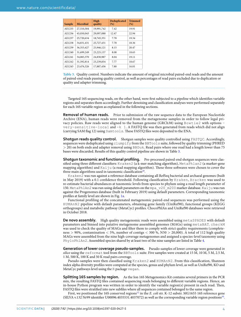
Shotgun reads quality control. Shotgun samples were quality controlled using FASTQC. Accordingly, sequences were deduplicated using clumpify from the BBTools suite, followed by quality trimming (PHRED > 20) on both ends and adapter removal using BBDuk. Read pairs where one read had a length lower than 75 bases were discarded. Results of this quality control pipeline are shown in Table 3.

Shotgun taxonomic and functional profiling. Pre-processed paired-end shotgun sequences were clas-sified using three different classifiers: Kraken2 (a k-mer matching algorithm), MetaPhlan2 (a marker-gene mapping algorithm) and Kaiju (a read mapping algorithm). These three softwares were chosen to cover the three main algorithms used in taxonomic classification20.

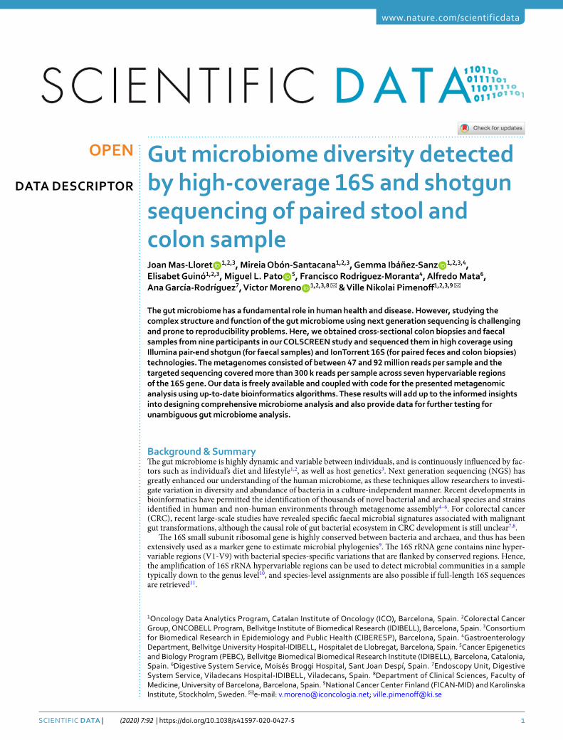
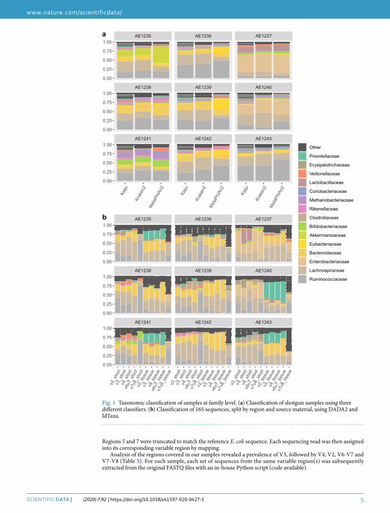
Kraken2 was run against a reference database containing all RefSeq bacterial and archaeal genomes (built in May 2019) with a 0.1 confidence threshold. Following classification by Kraken, Bracken was used to re-estimate bacterial abundances at taxonomic levels from species to phylum using a read length parameter of 150. MetaPhlAn2 was run using default parameters on the mpa_v20_m200 marker database. Kaiju was run against the Progenomes database (built in February 2019) using default parameters. Corresponding taxonomic profiles at family level are shown in Fig. 1a.

Functional profiling of the concatenated metagenomic paired-end sequences was performed using the HUMAnN2 pipeline with default parameters, obtaining gene family (UniRef90), functional groups (KEGG orthogroups) and metabolic pathway (MetaCyc) profiles. ChocoPhlAn and UniRef90 databases were retrieved in October 2018.

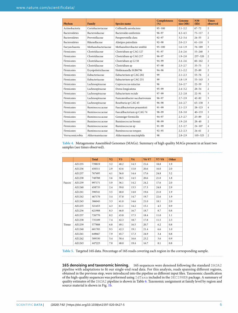
De novo assembly. High quality metagenomic reads were assembled using metaSPADES with default parameters and binned into putative metagenome assembled genomes (MAGs) using metaBAT. checkM was used to check the quality of MAGs and filter them to comply with strict quality requirements (complete-ness > 90%, contamination < 5%, number of contigs < 300 %, N50 > 20,000). A total of 112 high quality MAGs were assembled from the nine high-coverage metagenomes and assigned a species-level taxonomy using PhyloPhlAn2. Assembled species shared by at least two of the nine samples are listed in Table 4.

Generation of lower coverage pseudo-samples. Pseudo-samples of lower coverage were generated in silico using the reformat tool from the BBTools suite. Five samples were created at 15 M, 10 M, 5 M, 2.5 M, 1 M, 500 K, 100 K and 50 K read pairs coverage.

Pseudo-samples were then classified using Kraken2 and HUMAnN2. From this classification, Shannon index alpha diversity profiles were computed at the species, genus and phylum level, as well as UniRef90, KO and MetaCyc pathways level using the R package vegan.

Splitting 16S samples by region. As the Ion 16S Metagenomics Kit contains several primers in the PCR mix, the resulting FASTQ files contained sequencing reads belonging to different variable regions. Hence, an in-house Python program was written in order to identify the variable region(s) present in each read. Then, FASTQ files were stratified into new subfiles where all sequences contained belonged to the same region.

First, we positioned the 16S conserved regions12 in the E. coli str. K-12 substr. MG1655 16S reference gene (SILVA v.132 Nr99 identifier U00096.4035531.4037072) as well as the corresponding variable region positions10.

Sample MicrobialHigh quality

Deduplicated (%)

Trimmed (%)

AE1235 27,510,304 19,991,742 7.42 19.91

AE1236 45,050,043 29,097,088 12.47 22.94

AE1237 25,720,634 18,745,351 7.78 19.34

AE1238 34,831,431 25,727,431 7.78 18.36

AE1239 36,353,427 25,946,121 8.15 20.47

AE1240 31,699,249 23,225,137 8.08 18.65

AE1241 34,083,370 24,830,987 8.04 19.11

AE1242 31,592,814 23,239,834 7.77 18.67

AE1243 23,476,326 17,887,436 7.80 16.01

Table 3. Quality control. Numbers indicate the amount of original microbial paired-end reads and the amount of paired-end reads passing quality control, as well as percentages of read pairs excluded due to duplication or quality and adapter trimming.

5Scientific Data | (2020) 7:92 | https://doi.org/10.1038/s41597-020-0427-5

www.nature.com/scientificdatawww.nature.com/scientificdata/

Regions 5 and 7 were truncated to match the reference E. coli sequence. Each sequencing read was then assigned into its corresponding variable region by mapping.

Analysis of the regions covered in our samples revealed a prevalence of V3, followed by V4, V2, V6-V7 and V7-V8 (Table 5). For each sample, each set of sequences from the same variable region(s) was subsequently extracted from the original FASTQ files with an in-house Python script (code available).

AE1241 AE1242 AE1243

AE1238 AE1239 AE1240

AE1235 AE1236 AE1237

Kaiju

Krak

en2

Met

aPhl

An2

Kaiju

Krak

en2

Met

aPhl

An2

Kaiju

Krak

en2

Met

aPhl

An2

0.00

0.25

0.50

0.75

1.00

0.00

0.25

0.50

0.75

1.00

0.00

0.25

0.50

0.75

1.00

a

AE1241 AE1242 AE1243

AE1238 AE1239 AE1240

AE1235 AE1236 AE1237

v2_s

tool

v3_s

tool

v4_s

tool

v6v7

_sto

olv7

v8_s

tool

v2_t

issue

v3_t

issue

v4_t

issue

v6v7

_tiss

uev7

v8_t

issue

v2_s

tool

v3_s

tool

v4_s

tool

v6v7

_sto

olv7

v8_s

tool

v2_t

issue

v3_t

issue

v4_t

issue

v6v7

_tiss

uev7

v8_t

issue

v2_s

tool

v3_s

tool

v4_s

tool

v6v7

_sto

olv7

v8_s

tool

v2_t

issue

v3_t

issue

v4_t

issue

v6v7

_tiss

uev7

v8_t

issue

0.00

0.25

0.50

0.75

1.00

0.00

0.25

0.50

0.75

1.00

0.00

0.25

0.50

0.75

1.00

b

Other

Prevotellaceae

Erysipelotrichaceae

Veillonellaceae

Lactobacillaceae

Coriobacteriaceae

Methanobacteriaceae

Rikenellaceae

Clostridiaceae

Bifidobacteriaceae

Akkermansiaceae

Eubacteriaceae

Bacteroidaceae

Enterobacteriaceae

Lachnospiraceae

Ruminococcaceae

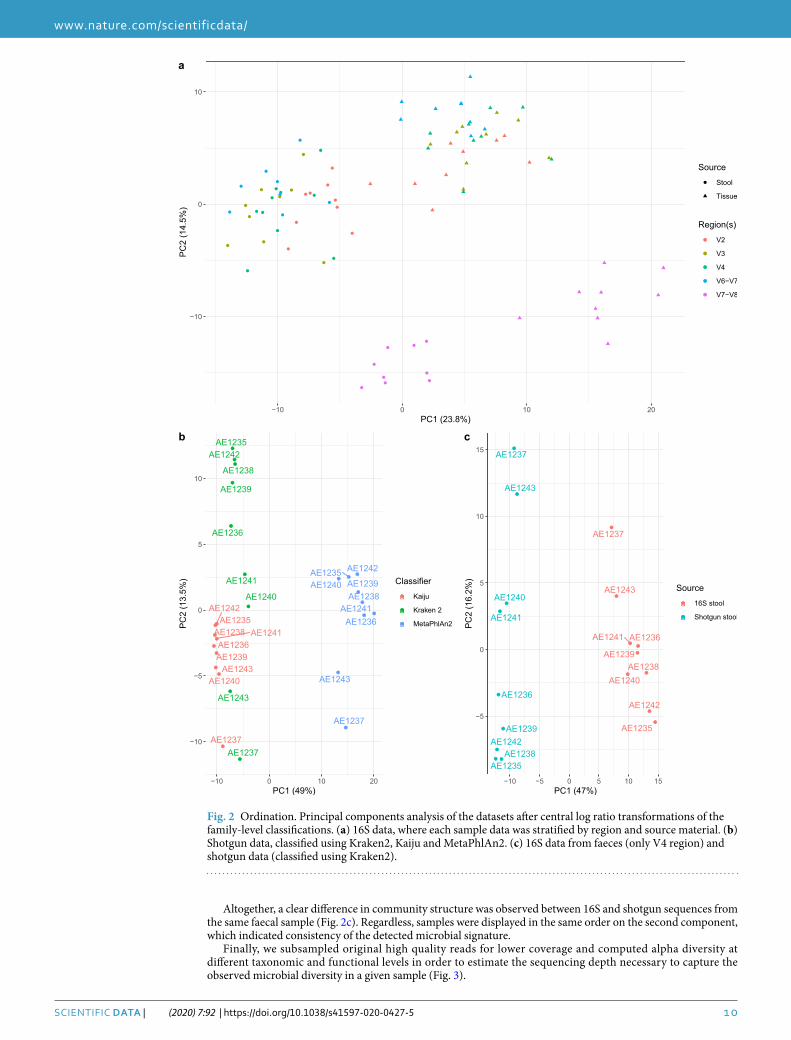
Fig. 1 Taxonomic classification of samples at family level. (a) Classification of shotgun samples using three different classifiers. (b) Classification of 16S sequences, split by region and source material, using DADA2 and IdTaxa.

6Scientific Data | (2020) 7:92 | https://doi.org/10.1038/s41597-020-0427-5

www.nature.com/scientificdatawww.nature.com/scientificdata/

16S denoising and taxonomic binning. 16S sequences were denoised following the standard DADA2 pipeline with adaptations to fit our single-end read data. For this analysis, reads spanning different regions, obtained in the previous step, were introduced into the pipeline as different input files. Taxonomic classification of the high-quality sequences was performed using IdTaxa included in the DECIPHER package. A summary of quality estimates of the DADA2 pipeline is shown in Table 6. Taxonomic assignment at family level by region and source material is shown in Fig. 1b.

Phylum Family Species nameCompleteness (%)

Genome size (Mb)

N50 (Kb)

Times observed

Actinobacteria Coriobacteriaceae Collinsella aerofaciens 95–100 2.1–2.2 67–72 2

Bacteroidetes Bacteroidaceae Bacteroides uniformis 96–97 4.2–4.5 75–117 2

Bacteroidetes Prevotellaceae Paraprevotella clara 92–97 3.2–3.4 24–55 2

Bacteroidetes Rikenellaceae Alistipes putredinis 92–98 2.0–2.3 61–110 5

Euryarchaeota Methanobacteriaceae Methanobrevibacter smithii 95–100 1.6–1.9 76–189 3

Firmicutes Clostridiaceae Clostridium sp CAG 127 91–97 2.4–2.6 53–240 3

Firmicutes Clostridiaceae Clostridium sp CAG 217 96–97 1.9–2.0 257–320 2

Firmicutes Clostridiaceae Clostridium sp L2 50 94–99 2.4–2.6 60–162 2

Firmicutes Clostridiaceae Clostridium sp 97–98 2.5–2.7 33–75 3

Firmicutes Erysipelotrichaceae Holdemanella SGB6796 94–96 2.1–2.2 25–89 2

Firmicutes Eubacteriaceae Eubacterium sp CAG 202 99 2.1–2.3 53–76 2

Firmicutes Eubacteriaceae Eubacterium sp CAG 251 99 1.8–1.9 53–143 3

Firmicutes Lachnospiraceae Coprococcus eutactus 96 2.6–2.7 22–59 2

Firmicutes Lachnospiraceae Dorea longicatena 95–99 2.4–3.2 28–54 2

Firmicutes Lachnospiraceae Eubacterium rectale 97–99 2.2–2.8 22–91 5

Firmicutes Lachnospiraceae Fusicatenibacter saccharivorans 96–97 2.7–2.9 42–82 3

Firmicutes Lachnospiraceae Roseburia sp CAG 45 96–98 2.6–2.7 63–138 3

Firmicutes Ruminococcaceae Faecalibacterium prausnitzii 91–99 2.1–2.5 28–123 4

Firmicutes Ruminococcaceae Faecalibacterium sp CAG 74 98–99 2.8–3.0 40–133 3

Firmicutes Ruminococcaceae Gemmiger formicilis 94–97 2.3–2.7 25–89 2

Firmicutes Ruminococcaceae Ruminococcus bromii 98–99 1.9–2.0 28–40 2

Firmicutes Ruminococcaceae Ruminococcus sp 91–99 2.3–2.7 24–107 4

Firmicutes Ruminococcaceae Ruminococcus torques 92–95 2.2–2.3 24–61 2

Verrucomicrobia Akkermansiaceae Akkermansia muciniphila 98 2.8–2.9 105–325 2

Table 4. Metagenome Assembled Genomes (MAGs). Summary of high quality MAGs present in at least two samples (see times observed).

Total V2 V3 V4 V6-V7 V7-V8 Other

Faeces

AE1235 739819 3.2 40.2 14.3 21.6 18.8 1.9

AE1236 450511 2.9 43.6 15.0 20.6 16.0 2.0

AE1237 767495 4.1 36.0 14.4 17.6 24.8 3.2

AE1238 740788 3.6 38.5 14.5 20.6 21.0 1.8

AE1239 997171 5.9 36.1 14.2 24.2 17.6 2.0

AE1240 458735 2.4 39.0 13.5 17.3 24.8 2.9

AE1241 590541 3.5 40.0 14.0 19.6 21.0 1.9

AE1242 467170 3.4 37.8 14.7 19.7 22.6 1.9

AE1243 386045 3.3 41.0 14.6 21.0 18.1 2.0

Tissue

AE1235 321453 4.3 61.1 14.2 15.1 4.5 0.9

AE1236 621908 8.3 46.8 16.7 18.7 8.7 0.8

AE1237 726770 8.2 43.8 17.5 18.4 11.0 1.1

AE1238 735109 7.4 42.3 18.7 17.8 11.5 2.3

AE1239 577808 6.8 49.1 16.5 20.7 6.2 0.8

AE1240 601785 9.5 42.3 19.1 21.4 6.6 1.0

AE1241 649667 7.9 45.7 17.3 24.9 3.4 0.8

AE1242 589330 5.4 50.4 16.6 23.2 3.6 0.9

AE1243 447223 7.0 48.0 19.4 16.7 8.1 0.8

Table 5. Targeted 16S data. Percentage of 16S reads covering each region in the corresponding sample.

7Scientific Data | (2020) 7:92 | https://doi.org/10.1038/s41597-020-0427-5

www.nature.com/scientificdatawww.nature.com/scientificdata/

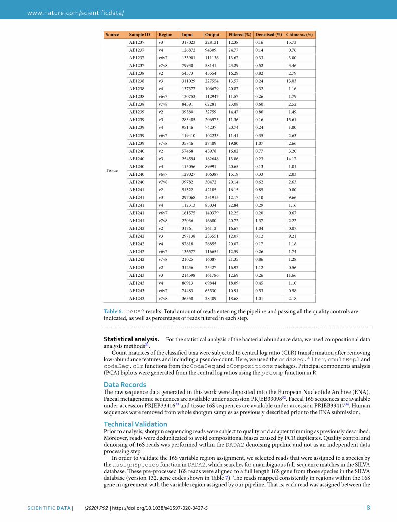
Source Sample ID Region Input Output Filtered (%) Denoised (%) Chimeras (%)

Stool

AE1235 v2 23675 18409 16.27 2.99 2.98

AE1235 v3 297069 204763 14.80 0.26 16.01

AE1235 v4 105530 72361 26.79 1.17 3.47

AE1235 v6v7 160139 118416 14.27 1.74 10.04

AE1235 v7v8 139431 102517 23.41 1.19 1.87

AE1236 v2 13177 10091 20.25 3.00 0.17

AE1236 v3 196436 148363 12.94 0.30 11.22

AE1236 v4 67353 46528 28.87 1.27 0.78

AE1236 v6v7 92647 71073 13.38 1.78 8.13

AE1236 v7v8 72100 55878 18.57 1.26 2.66

AE1237 v2 31697 22779 21.13 2.02 4.98

AE1237 v3 276040 201847 14.04 0.34 12.50

AE1237 v4 110375 82233 19.16 0.98 5.36

AE1237 v6v7 135004 91005 16.34 1.28 14.98

AE1237 v7v8 190178 126317 18.27 0.72 14.59

AE1238 v2 26631 21196 14.94 3.29 2.18

AE1238 v3 285027 206419 12.46 0.37 14.74

AE1238 v4 107172 80701 19.20 1.72 3.77

AE1238 v6v7 152748 111924 11.94 2.03 12.76

AE1238 v7v8 155514 111841 18.88 1.02 8.19

AE1239 v2 58730 46507 14.39 1.74 4.68

AE1239 v3 359574 251532 15.33 0.24 14.48

AE1239 v4 141973 103323 21.22 1.19 4.82

AE1239 v6v7 241379 173393 11.71 1.53 14.93

AE1239 v7v8 175774 130720 18.40 1.03 6.20

AE1240 v2 11200 8381 16.34 4.73 4.10

AE1240 v3 179016 123229 16.20 0.47 14.50

AE1240 v4 62106 47971 18.49 1.67 2.60

AE1240 v6v7 79313 50315 17.02 3.24 16.30

AE1240 v7v8 113851 83697 18.19 1.64 6.65

AE1241 v2 20533 15287 18.88 3.23 3.43

AE1241 v3 236319 164152 15.45 0.40 14.68

AE1241 v4 82470 62916 20.12 1.63 1.96

AE1241 v6v7 115842 83998 13.58 2.75 11.16

AE1241 v7v8 124095 89112 19.74 1.26 7.19

AE1242 v2 16093 12590 16.98 3.80 0.98

AE1242 v3 176603 116141 17.49 0.39 16.36

AE1242 v4 68441 51756 19.43 1.91 3.03

AE1242 v6v7 91881 67003 16.06 2.16 8.86

AE1242 v7v8 105442 81780 15.77 1.39 5.28

AE1243 v2 12651 9882 16.73 3.60 1.56

AE1243 v3 158164 112772 13.44 0.37 14.89

AE1243 v4 56432 40641 24.63 1.38 1.97

AE1243 v6v7 81212 57972 13.32 2.92 12.38

AE1243 v7v8 69949 52240 19.07 2.26 3.99

Tissue

AE1235 v2 13680 10741 18.41 1.69 1.39

AE1235 v3 196304 144394 11.75 0.23 14.46

AE1235 v4 45755 35944 20.18 0.42 0.84

AE1235 v6v7 48383 39295 15.96 0.67 2.16

AE1235 v7v8 14445 11208 21.16 0.97 0.28

AE1236 v2 51480 42622 15.80 0.50 0.91

AE1236 v3 291280 226960 11.57 0.16 10.35

AE1236 v4 103690 79166 22.58 0.21 0.86

AE1236 v6v7 116437 101656 11.56 0.19 0.94

AE1236 v7v8 53800 40664 20.83 0.57 3.01

AE1237 v2 59739 48980 14.92 0.61 2.47

Continued

8Scientific Data | (2020) 7:92 | https://doi.org/10.1038/s41597-020-0427-5

www.nature.com/scientificdatawww.nature.com/scientificdata/

Statistical analysis. For the statistical analysis of the bacterial abundance data, we used compositional data analysis methods31.

Count matrices of the classified taxa were subjected to central log ratio (CLR) transformation after removing low-abundance features and including a pseudo-count. Here, we used the codaSeq.filter, cmultRepl and codaSeq.clr functions from the CodaSeq and zCompositions packages. Principal components analysis (PCA) biplots were generated from the central log ratios using the prcomp function in R.

Data RecordsThe raw sequence data generated in this work were deposited into the European Nucleotide Archive (ENA). Faecal metagenomic sequences are available under accession PRJEB3309832. Faecal 16S sequences are available under accession PRJEB3341633 and tissue 16S sequences are available under accession PRJEB3341734. Human sequences were removed from whole shotgun samples as previously described prior to the ENA submission.

Technical ValidationPrior to analysis, shotgun sequencing reads were subject to quality and adapter trimming as previously described. Moreover, reads were deduplicated to avoid compositional biases caused by PCR duplicates. Quality control and denoising of 16S reads was performed within the DADA2 denoising pipeline and not as an independent data processing step.

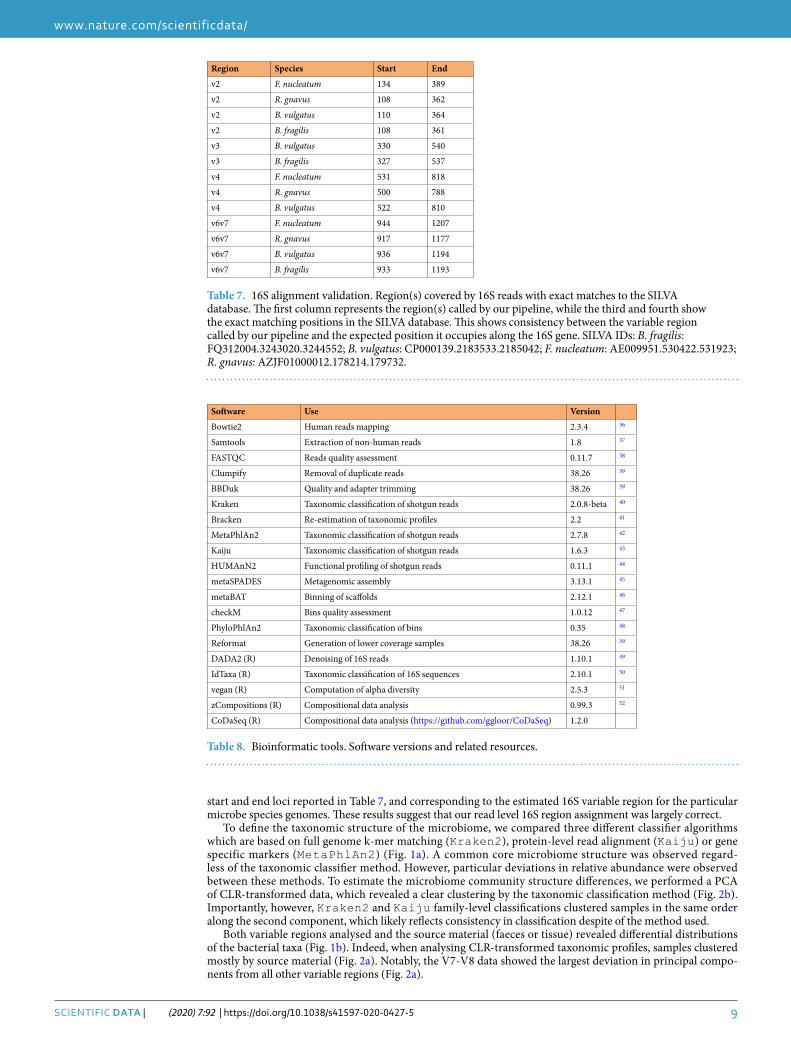
In order to validate the 16S variable region assignment, we selected reads that were assigned to a species by the assignSpecies function in DADA2, which searches for unambiguous full-sequence matches in the SILVA database. These pre-processed 16S reads were aligned to a full length 16S gene from those species in the SILVA database (version 132, gene codes shown in Table 7). The reads mapped consistently in regions within the 16S gene in agreement with the variable region assigned by our pipeline. That is, each read was assigned between the

Source Sample ID Region Input Output Filtered (%) Denoised (%) Chimeras (%)

Tissue

AE1237 v3 318023 228121 12.38 0.16 15.73

AE1237 v4 126872 94309 24.77 0.14 0.76

AE1237 v6v7 133901 111136 13.67 0.33 3.00

AE1237 v7v8 79930 58141 23.29 0.52 3.46

AE1238 v2 54373 43554 16.29 0.82 2.79

AE1238 v3 311029 227554 13.57 0.24 13.03

AE1238 v4 137377 106679 20.87 0.32 1.16

AE1238 v6v7 130753 112947 11.57 0.26 1.79

AE1238 v7v8 84391 62281 23.08 0.60 2.52

AE1239 v2 39380 32759 14.47 0.86 1.49

AE1239 v3 283485 206573 11.36 0.16 15.61

AE1239 v4 95146 74237 20.74 0.24 1.00

AE1239 v6v7 119410 102233 11.41 0.35 2.63

AE1239 v7v8 35846 27409 19.80 1.07 2.66

AE1240 v2 57468 45978 16.02 0.77 3.20

AE1240 v3 254594 182648 13.86 0.23 14.17

AE1240 v4 115056 89991 20.65 0.13 1.01

AE1240 v6v7 129027 106387 15.19 0.33 2.03

AE1240 v7v8 39782 30472 20.14 0.62 2.63

AE1241 v2 51322 42185 16.15 0.85 0.80

AE1241 v3 297068 231915 12.17 0.10 9.66

AE1241 v4 112313 85034 22.84 0.29 1.16

AE1241 v6v7 161575 140379 12.25 0.20 0.67

AE1241 v7v8 22036 16680 20.72 1.37 2.22

AE1242 v2 31761 26112 16.67 1.04 0.07

AE1242 v3 297138 233551 12.07 0.12 9.21

AE1242 v4 97818 76855 20.07 0.17 1.18

AE1242 v6v7 136577 116654 12.59 0.26 1.74

AE1242 v7v8 21025 16087 21.35 0.86 1.28

AE1243 v2 31236 25427 16.92 1.12 0.56

AE1243 v3 214598 161786 12.69 0.26 11.66

AE1243 v4 86913 69844 18.09 0.45 1.10

AE1243 v6v7 74483 65530 10.91 0.53 0.58

AE1243 v7v8 36358 28409 18.68 1.01 2.18

Table 6. DADA2 results. Total amount of reads entering the pipeline and passing all the quality controls are indicated, as well as percentages of reads filtered in each step.

9Scientific Data | (2020) 7:92 | https://doi.org/10.1038/s41597-020-0427-5

www.nature.com/scientificdatawww.nature.com/scientificdata/

start and end loci reported in Table 7, and corresponding to the estimated 16S variable region for the particular microbe species genomes. These results suggest that our read level 16S region assignment was largely correct.

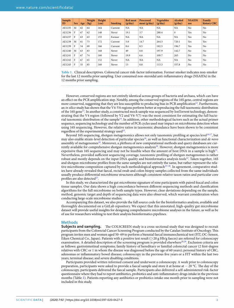
To define the taxonomic structure of the microbiome, we compared three different classifier algorithms which are based on full genome k-mer matching (Kraken2), protein-level read alignment (Kaiju) or gene specific markers (MetaPhlAn2) (Fig. 1a). A common core microbiome structure was observed regard-less of the taxonomic classifier method. However, particular deviations in relative abundance were observed between these methods. To estimate the microbiome community structure differences, we performed a PCA of CLR-transformed data, which revealed a clear clustering by the taxonomic classification method (Fig. 2b). Importantly, however, Kraken2 and Kaiju family-level classifications clustered samples in the same order along the second component, which likely reflects consistency in classification despite of the method used.

Both variable regions analysed and the source material (faeces or tissue) revealed differential distributions of the bacterial taxa (Fig. 1b). Indeed, when analysing CLR-transformed taxonomic profiles, samples clustered mostly by source material (Fig. 2a). Notably, the V7-V8 data showed the largest deviation in principal compo-nents from all other variable regions (Fig. 2a).

Software Use Version

Bowtie2 Human reads mapping 2.3.4 36

Samtools Extraction of non-human reads 1.8 37

FASTQC Reads quality assessment 0.11.7 38

Clumpify Removal of duplicate reads 38.26 39

BBDuk Quality and adapter trimming 38.26 39

Kraken Taxonomic classification of shotgun reads 2.0.8-beta 40

Bracken Re-estimation of taxonomic profiles 2.2 41

MetaPhlAn2 Taxonomic classification of shotgun reads 2.7.8 42

Kaiju Taxonomic classification of shotgun reads 1.6.3 43

HUMAnN2 Functional profiling of shotgun reads 0.11.1 44

metaSPADES Metagenomic assembly 3.13.1 45

metaBAT Binning of scaffolds 2.12.1 46

checkM Bins quality assessment 1.0.12 47

PhyloPhlAn2 Taxonomic classification of bins 0.35 48

Reformat Generation of lower coverage samples 38.26 39

DADA2 (R) Denoising of 16S reads 1.10.1 49

IdTaxa (R) Taxonomic classification of 16S sequences 2.10.1 50

vegan (R) Computation of alpha diversity 2.5.3 51

zCompositions (R) Compositional data analysis 0.99.3 52

CoDaSeq (R) Compositional data analysis (https://github.com/ggloor/CoDaSeq) 1.2.0

Table 8. Bioinformatic tools. Software versions and related resources.

Region Species Start End

v2 F. nucleatum 134 389

v2 R. gnavus 108 362

v2 B. vulgatus 110 364

v2 B. fragilis 108 361

v3 B. vulgatus 330 540

v3 B. fragilis 327 537

v4 F. nucleatum 531 818

v4 R. gnavus 500 788

v4 B. vulgatus 522 810

v6v7 F. nucleatum 944 1207

v6v7 R. gnavus 917 1177

v6v7 B. vulgatus 936 1194

v6v7 B. fragilis 933 1193

Table 7. 16S alignment validation. Region(s) covered by 16S reads with exact matches to the SILVA database. The first column represents the region(s) called by our pipeline, while the third and fourth show the exact matching positions in the SILVA database. This shows consistency between the variable region called by our pipeline and the expected position it occupies along the 16S gene. SILVA IDs: B. fragilis: FQ312004.3243020.3244552; B. vulgatus: CP000139.2183533.2185042; F. nucleatum: AE009951.530422.531923; R. gnavus: AZJF01000012.178214.179732.

1 0Scientific Data | (2020) 7:92 | https://doi.org/10.1038/s41597-020-0427-5

www.nature.com/scientificdatawww.nature.com/scientificdata/

Altogether, a clear difference in community structure was observed between 16S and shotgun sequences from the same faecal sample (Fig. 2c). Regardless, samples were displayed in the same order on the second component, which indicated consistency of the detected microbial signature.

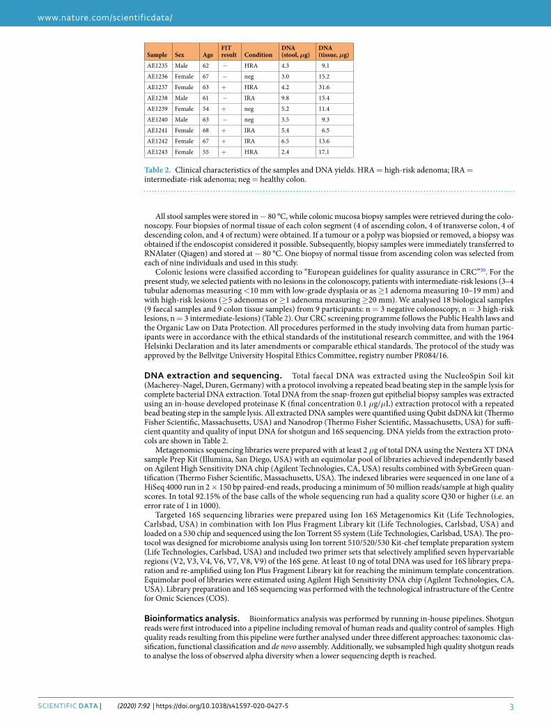
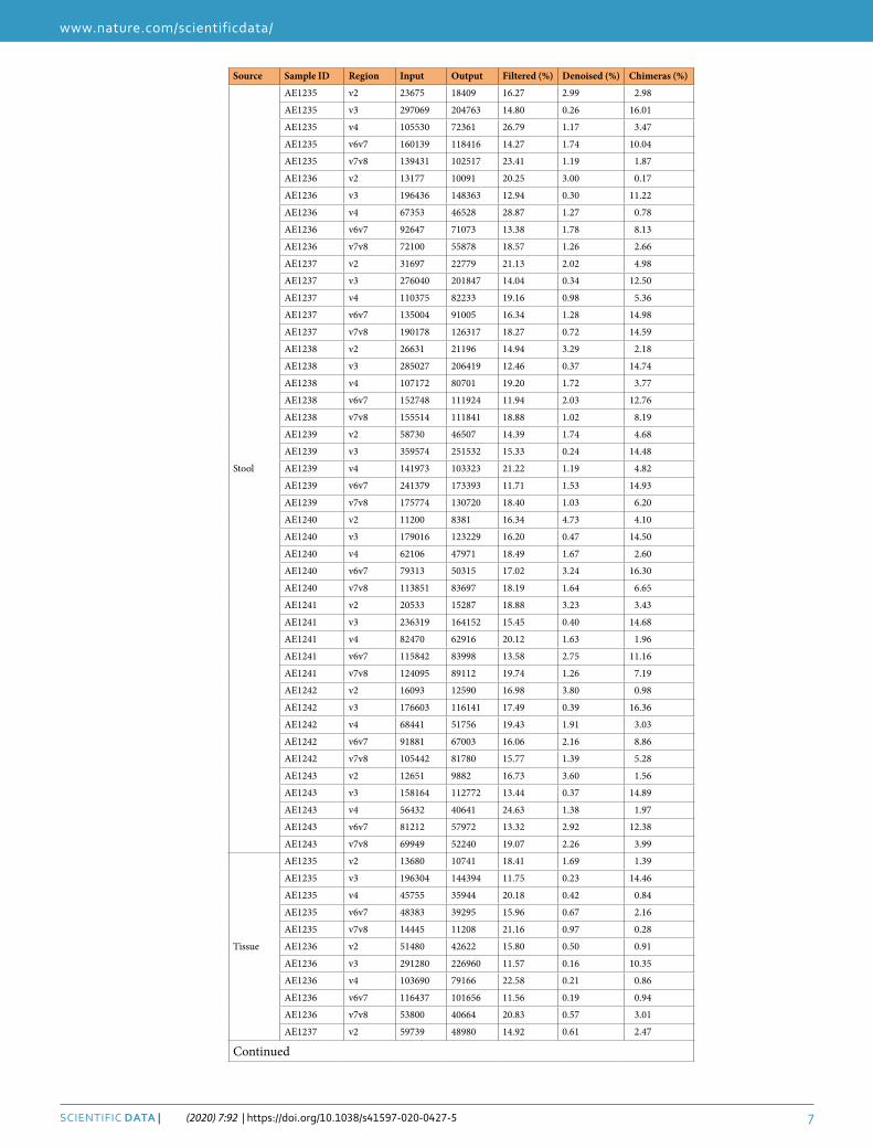
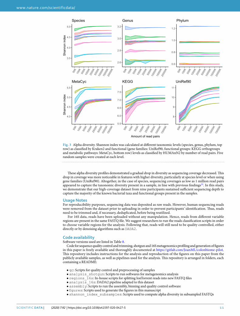
Finally, we subsampled original high quality reads for lower coverage and computed alpha diversity at different taxonomic and functional levels in order to estimate the sequencing depth necessary to capture the observed microbial diversity in a given sample (Fig. 3).

Fig. 2 Ordination. Principal components analysis of the datasets after central log ratio transformations of the family-level classifications. (a) 16S data, where each sample data was stratified by region and source material. (b) Shotgun data, classified using Kraken2, Kaiju and MetaPhlAn2. (c) 16S data from faeces (only V4 region) and shotgun data (classified using Kraken2).

1 1Scientific Data | (2020) 7:92 | https://doi.org/10.1038/s41597-020-0427-5

www.nature.com/scientificdatawww.nature.com/scientificdata/

These alpha diversity profiles demonstrated a gradual drop in diversity as sequencing coverage decreased. This drop in coverage was more noticeable in features with higher diversity, particularly at species level or when using gene families (UniRef90). Altogether, in the case of species, sequencing coverages as low as 1 million read pairs appeared to capture the taxonomic diversity present in a sample, in line with previous findings35. In this study, we demonstrate that our high-coverage dataset from nine participants sustained sufficient sequencing depth to capture the majority of the known bacterial taxa and functional groups present in the samples.

Usage NotesFor reproducibility purposes, sequencing data was deposited as raw reads. However, human sequencing reads were removed from the dataset prior to uploading in order to prevent participants’ identification. Thus, reads need to be trimmed and, if necessary, deduplicated, before being reutilized.

For 16S data, reads have been uploaded without any manipulation. Hence, reads from different variable regions are present in the same FASTQ file. We suggest researchers to run the reads classification scripts in order to choose variable regions for the analysis. Following that, reads will still need to be quality controlled, either directly or by denoising algorithms such as DADA2.

Code availabilitySoftware versions used are listed in Table 8.

Code for sequence quality control and trimming, shotgun and 16S metagenomics profiling and generation of figures in this paper is freely available and thoroughly documented at https://gitlab.com/JoanML/colonbiome-pilot. This repository includes instructions for the analysis and reproduction of the figures on this paper from the publicly available samples, as well as pipelines used for the analysis. This repository is arranged in folders, each containing a README:

• qc: Scripts for quality control and preprocessing of samples• analysis_shotgun: Scripts to run softwares for metagenomics analysis• regions_16s: In-house scripts for splitting IonTorrent reads into new FASTQ files• analysis_16s: DADA2 pipeline adapted to this dataset• assembly: Scripts to run the assembly, binning and quality control software• figures: Scripts used to generate the figures in this manuscript• shannon_index_subsamples: Scripts used to compute alpha diversity in subsampled FASTQs

3.5

4.0

4.5

5.0

50K

100K

500K

1000

K25

00K

5000

K10

000K

1500

0K20

000K

Sha

nnon

inde

x

Species

2.6

2.8

3.0

3.2

50K

100K

500K

1000

K25

00K

5000

K10

000K

1500

0K20

000K

Genus

0.6

0.8

1.0

1.2

50K

100K

500K

1000

K25

00K

5000

K10

000K

1500

0K20

000K

Phylum

4.0

4.5

5.0

5.5

50K

100K

500K

1000

K25

00K

5000

K10

000K

1500

0K

Sha

nnon

inde

x

MetaCyc

5.5

6.0

6.5

7.0

7.5

50K

100K

500K

1000

K25

00K

5000

K10

000K

1500

0K

Amount of read pairs

KEGG

8

9

10

11

50K

100K

500K

1000

K25

00K

5000

K10

000K

1500

0K

UniRef90

Fig. 3 Alpha diversity. Shannon index was calculated at different taxonomic levels (species, genus, phylum, top row) as classified by Kraken2 and functional (gene families: UniRef90, functional groups: KEGG orthogroups and metabolic pathways: MetaCyc, bottom row) levels as classified by HUMAnN2 by number of read pairs. Five random samples were created at each level.

1 2Scientific Data | (2020) 7:92 | https://doi.org/10.1038/s41597-020-0427-5

www.nature.com/scientificdatawww.nature.com/scientificdata/

Received: 13 September 2019; Accepted: 21 February 2020;Published: xx xx xxxx

References 1. Maier, L. & Typas, A. Systematically investigating the impact of medication on the gut microbiome. Curr. Opin. Microbiol. 39,

128–135 (2017). 2. Maier, L. et al. Extensive impact of non-antibiotic drugs on human gut bacteria. Nature 555, 623–628 (2018). 3. Goodrich, J. K., Davenport, E. R., Clark, A. G. & Ley, R. E. The Relationship Between the Human Genome and Microbiome Comes

into View. Annu. Rev. Genet. 51, 413–433 (2017). 4. Parks, D. H. et al. Recovery of nearly 8,000 metagenome-assembled genomes substantially expands the tree of life. Nat. Microbiol. 2,

1533–1542 (2017). 5. Almeida, A. et al. A new genomic blueprint of the human gut microbiota. Nature 568, 499–504 (2019). 6. Pasolli, E. et al. Extensive Unexplored Human Microbiome Diversity Revealed by Over 150,000 Genomes from Metagenomes

Spanning Age, Geography, and Lifestyle. Cell 176, 649–662.e20 (2019). 7. Wirbel, J. et al. Meta-analysis of fecal metagenomes reveals global microbial signatures that are specific for colorectal cancer. Nat.

Med 25, 679–689 (2019). 8. Thomas, A. M. et al. Metagenomic analysis of colorectal cancer datasets identifies cross-cohort microbial diagnostic signatures and

a link with choline degradation. Nat. Med. 25, 667–678 (2019). 9. Weisburg, W. G., Barns, S. M., Pelletier, D. A. & Lane, D. J. 16S ribosomal DNA amplification for phylogenetic study. J. Bacteriol. 173,

697–703 (1991). 10. Yarza, P. et al. Uniting the classification of cultured and uncultured bacteria and archaea using 16S rRNA gene sequences. Nat. Rev.

Microbiol. 12, 635–645 (2014). 11. Edgar, R. C. Updating the 97% identity threshold for 16S ribosomal RNA OTUs. Bioinformatics 34, 2371–2375 (2018). 12. Martinez-Porchas, M., Villalpando-Canchola, E., OrtizSuarez, L. E. & Vargas-Albores, F. How conserved are the conserved

16S-rRNA regions? PeerJ 5, e3036 (2017). 13. Yang, B., Wang, Y. & Qian, P. Y. Sensitivity and correlation of hypervariable regions in 16S rRNA genes in phylogenetic analysis.

BMC Bioinformatics 17, 1–8 (2016). 14. Barb, J. J. et al. Development of an Analysis Pipeline Characterizing Multiple Hypervariable Regions of 16S rRNA Using Mock

Samples. PLoS ONE 11, 1–18 (2016). 15. D’Amore, R. et al. A comprehensive benchmarking study of protocols and sequencing platforms for 16S rRNA community profiling.

BMC Genomics 17, 55 (2016). 16. Lindgreen, S., Adair, K. L. & Gardner, P. P. An evaluation of the accuracy and speed of metagenome analysis tools. Sci. Rep. 6, 1–14

(2016). 17. McIntyre, A. B. et al. Comprehensive benchmarking and ensemble approaches for metagenomic classifiers. Genome Biol. 18, 1–19

(2017). 18. Truong, D. T., Tett, A., Pasolli, E., Huttenhower, C. & Segata, N. Microbial strain-level population structure and genetic diversity

from metagenomes. Genome Res. 27, 626–638 (2017). 19. van der Walt, A. J. et al. Assembling metagenomes, one community at a time. BMC Genomics 18, 1–13 (2017). 20. Breitwieser, F. P., Lu, J. & Salzberg, S. L. A review of methods and databases for metagenomic classification and assembly. Brief.

Bioinform. 20(4), 1125–1136 (2017). 21. Vincent, A. T., Derome, N., Boyle, B., Culley, A. I. & Charette, S. J. Next-generation sequencing (NGS) in the microbiological world:

How to make the most of your money. J. Microbiol. Methods 138, 60–71 (2017). 22. Walsh, A. M. et al. Species classifier choice is a key consideration when analysing low-complexity food microbiome data. Microbiome

6, 50 (2018). 23. Clooney, A. G. et al. Comparing apples and oranges?: Next generation sequencing and its impact on microbiome analysis. PLoS ONE

11, 1–16 (2016). 24. Jovel, J. et al. Characterization of the gut microbiome using 16S or shotgun metagenomics. Front. Microbiol. 7, 1–17 (2016). 25. Tessler, M. et al. Large-scale differences in microbial biodiversity discovery between 16S amplicon and shotgun sequencing. Sci. Rep.

7, 1–14 (2017). 26. Laudadio, I. et al. Quantitative Assessment of Shotgun Metagenomics and 16S rDNA Amplicon Sequencing in the Study of Human

Gut Microbiome. OMICS 22, 248–254 (2018). 27. Jones, R. B. et al. Inter-niche and inter-individual variation in gut microbial community assessment using stool, rectal swab, and

mucosal samples. Sci. Rep. 8, 1–12 (2018). 28. Peris, M. et al. Lessons learnt from a population-based pilot programme for colorectal cancer screening in Catalonia (Spain). J. Med.

Screen. 14, 81–86 (2007). 29. Binefa, G. et al. Colorectal Cancer Screening Programme in Spain: Results of Key Performance Indicators after Five Rounds (2000-

2012). Sci. Rep. 6, 1–10 (2016). 30. Atkin, W. S. et al. European guidelines for quality assurance in colorectal cancer screening and diagnosisFirst Edition Colonoscopic

surveillance following adenoma removal. Endoscopy 44, 151–163 (2012). 31. Gloor, G. B., Macklaim, J. M., Pawlowsky-Glahn, V. & Egozcue, J. J. Microbiome Datasets Are Compositional: And This Is Not

Optional. Front. Microbiol. 8, 2224 (2017). 32. European Nucleotide Archive, https://identifiers.org/ena.embl:PRJEB33098 (2019). 33. European Nucleotide Archive, https://identifiers.org/ena.embl:PRJEB33416 (2019). 34. European Nucleotide Archive, https://identifiers.org/ena.embl:PRJEB33417 (2019). 35. Hillmann, B. et al. Evaluating the Information Content of Shallow Shotgun Metagenomics. mSystems 3, 1–12 (2018). 36. Langmead, B. & Salzberg, S. L. Fast gapped-read alignment with Bowtie 2. Nat. Methods 9, 357–359 (2012). 37. Li, H. et al. The Sequence Alignment/Map format and SAMtools. Bioinformatics 25, 2078–9 (2009). 38. FASTQC (Babraham Institute, 2018). 39. BBTools v.38.26 (Joint Genome Institute, 2018). 40. Wood, D. E., Lu, J. & Langmead, B. Improved metagenomic analysis with Kraken 2. Genome Res. 20, 257 (2019). 41. Lu, J., Breitwieser, F. P., Thielen, P. & Salzberg, S. L. Bracken: estimating species abundance in metagenomics data. PeerJ 3, e104

(2017). 42. Truong, D. T. et al. MetaPhlAn2 for enhanced metagenomic taxonomic profiling. Nat. Methods 12, 902–903 (2015). 43. Menzel, P., Ng, K. L. & Krogh, A. Fast and sensitive taxonomic classification for metagenomics with Kaiju. Nat. Commun. 7, 1–9

(2016). 44. Franzosa, E. A. et al. Species-level functional profiling of metagenomes and metatranscriptomes. Nat. Methods 15, 962–968 (2018). 45. Nurk, S., Meleshko, D., Korobeynikov, A. & Pevzner, P. A. metaSPAdes: a new versatile metagenomic assembler. Genome Res. 27,

824–834 (2017). 46. Kang, D. et al. MetaBAT 2: an adaptive binning algorithm for robust and efficient genome reconstruction from metagenome

assemblies. PeerJ e7359 (2019).

13Scientific Data | (2020) 7:92 | https://doi.org/10.1038/s41597-020-0427-5

www.nature.com/scientificdatawww.nature.com/scientificdata/

47. Parks, D. H., Imelfort, M., Skennerton, C. T., Hugenholtz, P. & Tyson, G. W. CheckM: assessing the quality of microbial genomes recovered from isolates, single cells, and metagenomes. Genome Res. 25, 1043–55 (2015).

48. Segata, N., Börnigen, D., Morgan, X. C. & Huttenhower, C. PhyloPhlAn is a new method for improved phylogenetic and taxonomic placement of microbes. Nat. Commun. 4, 2304 (2013).

49. Callahan, B. J. et al. DADA2: High-resolution sample inference from Illumina amplicon data. Nat. Methods 13, 581–583 (2016). 50. Murali, A., Bhargava, A. & Wright, E. S. IDTAXA: A novel approach for accurate taxonomic classification of microbiome sequences.

Microbiome 6, 1–14 (2018). 51. Oksanen, J. et al. vegan: Community Ecology Package. https://CRAN.R-project.org/package=vegan. R package version 2.5-5 (2019). 52. Palarea-Albaladejo, J. & Martín-Fernández, J. A. zCompositions — R package for multivariate imputation of left-censored data

under a compositional approach. Chemometr. Intell. Lab. Systems 143, 85–96 (2015).

AcknowledgementsWe appreciate the collaboration of all participants who provided epidemiological data and biological samples. We thank all the personnel that were involved in the recruitment process, specially our documentalist Carmen Atencia and our laboratory technician Susana López. This research was financially supported by the Ministry of Science, Innovation and Universities, Government of Spain (grant FPU17/05474). Ministry of Health, Government of Catalonia (grants SLT002/16/00496 and SLT002/16/00398), Spanish Ministry for Economy and Competitivity, Instituto de Salud Carlos III, co-funded by FEDER funds -a way to build Europe- (FIS PI17/00092), Agency for Management of University and Research Grants (AGAUR) of the Catalan Government (grant 2017SGR723). Mireia Obón-Santacana received a post-doctoral fellow from "Fundación Científica de la Asociación Española Contra el Cáncer (AECC)”. We thank CERCA Program, Generalitat de Catalunya for institutional support. None of these agencies had any role in the interpretation of the results or the preparation of this manuscript. Open access funding provided by Karolinska Institute.

Author contributionsV.P. and V.M. designed and supervised the study. G.I.S., E.G. and M.O.S. designed the recruitment protocols. G.I.S., F.R.M., A.M. and A.G.R. conducted the recruitment and sample collection. M.L.P. contributed to the sample preparation and sequencing protocols. J.M.L. conducted the bioinformatics analysis. J.M.L. and V.P. interpreted the analysis and wrote the first draft of the manuscript. All co-authors assisted in the writing of the manuscript and approved the submitted version.

Competing interestsThe authors declare no competing interests.

Additional informationCorrespondence and requests for materials should be addressed to V.M. or V.N.P.Reprints and permissions information is available at www.nature.com/reprints.Publisher’s note Springer Nature remains neutral with regard to jurisdictional claims in published maps and institutional affiliations.

Open Access This article is licensed under a Creative Commons Attribution 4.0 International License, which permits use, sharing, adaptation, distribution and reproduction in any medium or

format, as long as you give appropriate credit to the original author(s) and the source, provide a link to the Cre-ative Commons license, and indicate if changes were made. The images or other third party material in this article are included in the article’s Creative Commons license, unless indicated otherwise in a credit line to the material. If material is not included in the article’s Creative Commons license and your intended use is not per-mitted by statutory regulation or exceeds the permitted use, you will need to obtain permission directly from the copyright holder. To view a copy of this license, visit http://creativecommons.org/licenses/by/4.0/.

The Creative Commons Public Domain Dedication waiver http://creativecommons.org/publicdomain/zero/1.0/ applies to the metadata files associated with this article. © The Author(s) 2020