Guns and Roses: Flower Exports and Electoral Violence in Kenya

Guns and Roses: Flower Exports and

Electoral Violence in Kenya

Christopher Ksoll∗ Rocco Macchiavello† Ameet Morjaria‡

June 2014§

Abstract

This paper studies how firms react to electoral violence. Predictions derived from amodel of firms reaction to violence are tested using Kenya flower exporters during the2008 post-election violence. The violence reduced exports primarily through workersabsence and had heterogenous effects: firms with direct contractual relationships inexport markets and members of the business association had higher incentives andlower costs of reacting to the violence and suffered smaller production and workerslosses. Model calibrations suggest that the average firm operated at a loss during theviolence and absent workers suffered welfare losses at least three times larger thanweekly earnings. The results show how the impact of violence on trade is mediated bydifferent institutional arrangements associated with export.

∗University of Oxford; Email: [email protected].†Warwick University, BREAD and CEPR; E-mail: [email protected]‡Harvard University; Email: [email protected]§We thank Oriana Bandiera, Tim Besley, Chris Blattman, Robin Burgess, Stefan Dercon, Marcel

Fafchamps, Maitreesh Ghatak, Asim Khwaja, Eliana LaFerrara, Guy Michaels, Torsten Persson, FabianWaldinger, Chris Woodruff and conference and seminar participants at CalTech, CSAE 2009, LSE, Manch-ester, Mannheim, NEUDC 2009, Oxford and Simon Fraser for helpful comments and suggestions. Weacknowledge funding from iiG as part of the UK Department for International Development (DFID).Theviews expressed are not necessarily those of DFID. Financial support from George Webb Medley/OxfordEconomic Papers fund is gratefully acknowledged. Ameet Morjaria would like to thank STICERD andNSF-IGC-AERC for a travel award and EDRI for hosting his stay in Ethiopia.

1

1 Introduction

This paper studies the effects of electoral violence on an export oriented industry. Export

development is important to promote growth and poverty reduction in low income countries

(see, e.g., Rodrik (2005)). In many countries, however, growth and exports are hindered by

instability and frequent disruptions in production. In the African context, violent conflicts,

particularly at election times, are a common cause of instability and disruption in production

(see, e.g., Bates (2001, 2008)). During the period from 1990 to 2007, 19% of the 213 elections

which took place in Sub-Saharan Africa witnessed electoral violence (see Straus and Taylor

(2009) and Table [A1] for an update).1

An expanding body of evidence from cross-country studies (see, e.g., Alesina et al.

(1996), Collier (2007), Glick and Taylor (2010)) shows that violent conflicts has negative

effects on growth, investment and trade at the macro level. While necessary to understand

the channels through which violence affects firms and formulate appropriate policies, micro-

level evidence on the impact of violence on firms’ operations, however, remains scarce. There

are two major empirical challenges to provide micro-level evidence: i) gathering detailed

information on the operations of firms before, during and after the violent conflict, and ii)

constructing a valid counterfactual, i.e., assessing what would have happened to the firms in

the absence of the violence.

This paper investigates the mechanisms and costs of disruptions induced by the post-

electoral violence in 2008 on Kenyan floriculture, one of the largest earner of foreign currency

and employer of poorly educated women in rural areas. The setting of this study allows

to overcome the two empirical challenges identified above. Kenyan flowers are produced

almost exclusively for the export market. Daily data on exports, available from customs

records at the firm level before, during and after the violence, match day-by-day production

activity on the farms. Moreover, flowers are grown and exported by vertically integrated

firms and, therefore, the export data can also be matched with the exact location where

flowers are produced.2 The ethnic violence that followed the elections in Kenya at the end

1Straus and Taylor (2009) list cases with twenty or more deaths. For comparison, Blattman and Miguel(2009) define civil wars as internal conflicts that count more than 1,000 battle deaths in a single year andcivil conflicts as those that count at least 25 deaths per annum. The International Foundation for ElectoralSystems (IFES) defines “election violence [a]s any harm or threat to any person or property involved in theelection process, or to the election process itself, during the election period” (see http://www.ifes.org).

2Other perishable agricultural products, instead, are grown in rural areas and then processed and exportedby firms located in the larger towns of Nairobi and Mombasa. This precludes matching production withlocation. For other sectors, e.g., most manufacturing, that are not primarily involved in exports, accuratehigh-frequency data on production or sales do not exist.

2

of 2007 did not equally affect all regions of the country where flower firms are located. The

detailed information on the time and location of production, therefore, can be combined

with spatial and temporal variation in the incidence of the violence to construct several

appropriate counterfactuals to assess the causal impact of the violence on production. The

data, in particular, allow us to estimate firm-specific reduced form effect of the violence on

production that control for both seasonality and growth effects.

We complemented the administrative data by designing and conducting a survey of

flower firms in Kenya shortly after the end of the violence. The survey collected information

on how firms were affected by and reacted to the violence. Beside underpinning the formu-

lation of a theoretical model of a firm’s reaction to the violence, the survey is combined with

the administrative data to shed light on the mechanisms through which the violence affected

the firms. Finally, the combination of firm-specific reduced form estimates obtained from the

administrative records with information collected through the survey allows us to calibrate

the model and construct bounds on firms’ losses and on the costs incurred by workers due

to the violence.

The results show that, after controlling for firm-specific seasonality and growth pat-

terns, weekly export volumes of firms in the affected regions dropped, on average, by 38%

relative to what would have happened had the violence not occurred. Guided by the pre-

dictions of the model, we investigate the mechanisms through which the violence affected

the firms and show two sets of results. First, the evidence shows that workers’ absence,

which across firms averaged 50% of the labor force at the peak of the violence, was the

main channel through which the violence affected production, rather than transportation

problems. Second, we explore sources of heterogeneity in both firms’ exposure and response

to the violence. Within narrowly defined locations, we find that large firms and firms with

stable contractual relationships in export markets registered smaller proportional losses in

production and reported proportionally fewer workers absent during the time of the violence.

These results hold even after controlling for characteristics of the labor force (gender, edu-

cation, ethnicity), working arrangements (percentage of seasonal vs. permanent employees,

housing programs on the farm, fair trade certification) and ownership (foreign, politically

connected).3 We also find that firms affiliated with the industry business association suffered

lower reductions in export volumes. Perhaps surprisingly, after accounting for these char-

acteristics, we find no evidence that foreign-owned firms, firms more closely connected to

3Consistent with the theoretical predictions, once workers’ absence is directly controlled for, the location,size and marketing channels of the firms do not explain production losses.

3

politicians, or fair trade certified firms suffered differential reductions in exports and workers

losses. Taken together, the evidence suggests that institutional arrangements developed to

export in integrated non-traditional agricultural value chains gave firms higher incentives to

react and limit the disruptions caused by the violence.

Firms responded to the violence by compensating the workers that came to work

for the (opportunity) costs of coming to work during the violence period and by increasing

working hours to keep up production despite severe workers absence. As a result, despite

the temporary reduction in the labor force, the calibration exercise reveals that the weekly

wage bill during the violence period increased by 70% for the average firm. This provides a

lower bound to the increase in costs since it does not include other expenses, such as hiring

of security, extra-inputs, etc. Even taking into account the 10% depreciation of the Kenyan

shilling, the lower revenue and cost increases suggest that the average firm operated at a loss

during the period of the violence.

Workers who did attend work were compensated by the firms for the opportunity cost

of going to work. However, at the average firm, about 50% of the labor force did not come to

work for at least one week during the period of the violence. Those absent had higher costs

of going to work during the violence; and the calibration exercise suggests that these costs

were more than three times higher than normal weekly earnings for the marginal worker.

The estimates, therefore, suggest large welfare costs of the violence on workers.

The findings from this study are relevant to countries interested in fostering non-

traditional agricultural value chains.4 In particular, the incentives associated with inte-

grated value chains in non-traditional agriculture and a well-functioning business association

enabled firms to quickly respond to the violence through both horizontal and vertical coor-

dination along the supply chain. This also suggests that even larger negative effects might

be expected in traditional agriculture value chains in which domestic traders and proces-

sors market the fresh produce of smaller farmers, often for the local market. Second, as in

our study, even in contexts characterized by intense and prolonged episodes of violence, the

available evidence suggests that the most important effects of violence on firms are caused by

the flight of employees and the unreliability of transport, rather than by physical destruction

(see, e.g., Collier and Duponchel (2010) for Sierra Leone).

This work thus provides firm-level evidence on the mechanisms that underpin the

4In many African countries, export revenues are very highly concentrated in few primary, includingagricultural, sectors. The success of floriculture in Kenya has led several other Sub-Saharan countries, mostnotably Ethiopia, but also Tanzania, Uganda and others, to promote the development of the industry.

4

impacts of conflict on international trade. The existing literature has studied trade disrup-

tions at a more aggregate level. For instance, Glick and Taylor (2010) show that wars affect

not only the parties directly affected, but also trade with third parties, while Nitsch and

Schumacher (2004) show that terrorism within a country affects trade with other countries.5

Our paper documents that the institutional arrangements used by firms to participate in

international value chains are important in determining the impact of conflict on trade. In

doing so, it adds to a handful of papers providing micro-level evidence on the relationship

between conflict and firms.6 The closest work to ours is that of Abadie and Gardeazabal

(2003) and of Guidolin and La Ferrara (2007), both of which also look at a particular conflict.

Abadie and Gardeazabal (2003) study the impact of the Basque terrorist conflict on growth

in the Basque region by constructing a counterfactual region and compare the growth of that

counterfactual region to the actual growth experience of the Basque country. They then look

at stock market returns of firms who operated in the Basque region when the terrorist orga-

nization announced a truce and find that the announcement of the cease-fire led to excess

returns for firms operating in the Basque region. Guidolin and La Ferrara (2007) conduct an

event study of the sudden end of the civil conflict in Angola, which was marked by the death

of the rebel movement leader in 2002. They find that the stock market perceived this event

as “bad news” for the diamond companies holding concessions there. The main difference

between these papers and ours is that our study provides evidence on the effect of conflict on

firms using firm-level export and survey records, rather than stock-market data. In contrast

to stock market reactions, our data allow us to unpack the various channels through which

the violence has affected firms’ operations. Furthermore, combining the reduced form esti-

mates with survey evidence, we are able to back out lower bounds to the profits and workers

welfare losses caused by the violence. Dube and Vargas (2007) provide micro-evidence on

the relationship between export and violence in Colombia. They find that an increase in the

international price of labor-intensive export commodity reduces violence while an increase

in the international price of a capital-intensive export good increases violence. We do not

investigate the channel through which investment, production and exports in the flower in-

dustry might have affected the conflict; instead, we condition on locations in which flowers

5Collier and Hoeffler (1998), Besley and Persson (2008) and Martin et al. (2008) provide further examplesof macro-level evidence on the relationship between trade and civil conflict.

6Almost all papers in the microeconomic literature of violence and civil conflict focus on the impactsof conflict on investment in human capital and children, e.g., Akresh and De Walque (2009), Blattmanand Annan (2010), Leon (2010) and Miguel and Roland (2010). This part of the literature is surveyed inBlattman and Miguel (2009).

5

are already grown and study the response of producers to the violence. Finally, Dercon and

Romero-Gutierrez (2010) and Dupas and Robinson (2010) provide survey-based evidence of

the violence that followed the Kenyan presidential elections. Dupas and Robinson (2010),

in particular, find, consistently with the results in this paper, large effects of the violence

on income, consumption and expenditures on a sample of sex-workers and shopkeepers in

Western Kenya.

The remainder of the paper is organized as follows. Section 2 provides some back-

ground information on the Kenyan flower industry, the post-electoral violence and describes

the data. Section 3 presents the theoretical framework. Section 4 presents the estimation

strategy and empirical results. Section 5 offers some concluding remarks.

2 Background and Data

2.1 Kenyan Flower Industry

In the last decade Kenya has become one of the leading exporters of flowers in the world

overtaking traditional producers such as Israel, Colombia and Ecuador. Exports of cut

flowers are among the largest sources of foreign currency for Kenya alongside tourism and

tea. The Kenyan flower industry counts around one hundred established exporters located

in various clusters in the country.

Since flowers are a fragile and highly perishable commodity, growing flowers for ex-

ports is a complex business. In order to ensure the supply of high-quality flowers to distant

markets, coordination along the supply chain is crucial. Flowers are hand-picked in the field,

kept in cool storage rooms at constant temperature for grading, then packed, transported to

the airport in refrigerated trucks, inspected and sent to overseas markets. The industry is

labor intensive and employs mostly low-educated women in rural areas. The inherent per-

ishable nature of the flowers implies that post-harvest care is a key determinant of quality.

Workers, therefore, receive significant training in harvesting, handling, grading and pack-

ing, acquiring skills that are difficult to replace in the short-run. Because of both demand

(e.g., particular dates such as Valentines’ Day and Mother’s Day) and supply factors (it is

costly to produce flowers in Europe during winter), floriculture is a business characterized by

significant seasonality. Flowers are exported from Kenya either through the Dutch auctions

located in the Netherlands, or through direct sales to wholesalers and/or specialist importers.

In the first case, the firm has no control over the price and has no contractual obligations for

6

delivery. In the latter, instead, the relationship between the exporter and the foreign buyer

is governed through a (non-written) relational contract.

2.2 Electoral Violence

Kenya’s fourth multi-party general elections were held on the 27th of December 2007 and

involved two main candidates: the incumbent Mwai Kibaki was running for a re-election, a

Kikuyu hailing from the Central province representing the Party of National Unity (PNU),

and Raila Odinga a Luo from the Nyanza province representing the main opposition party,

the Orange Democratic Movement (ODM). The support bases for the two opposing coalitions

were clearly marked along ethnic lines (see Kimenyi and Shughart (2010), Bratton and

Kimenyi (2008) and Gibson and Long (2009)).

Polls leading up to the elections showed that the race would be close. Little violence

occurred on election day, and observers considered the voting process orderly. Exit polls

gave a comfortable lead to the challenger, Odinga, by as much as 50% against 40% for

Kibaki. The challengers led on the first day of counting (28th, December) lead to an initial

victory declaration by ODM (29th, December). However on the 29th, the head of the Electoral

Commission of Kenya declared Kibaki the winner, by a margin of 2%. The hasty inauguration

of Kibaki on the afternoon of the 30th December resulted in Odinga accusing the government

of fraud.7 Within minutes of the announcements of the election results, a political and

humanitarian crisis erupted nationwide. Targeted ethnic violence broke out in various parts

of the country where ODM supporters, especially in Nyanza, Mombasa, Nairobi and parts of

the Rift Valley, targeted Kikuyus who were living outside their traditional settlement areas

of the Central province. This first outburst of violence, which lasted for a few days, was

followed by a second outbreak of violence between the 25th and the 30th of January. This

second phase of violence happened mainly in the areas of Nakuru, Naivasha and Limuru

as a revenge attack on ODM supporters.8 Sporadic violence and chaos continued until a

power sharing agreement was reached on the 29th of February. By the end of the violence

some 1,200 people had died in the clashes and at least 500,000 were displaced and living

in internally displaced camps (Gibson and Long (2009)). The economic effects of the crisis

7According to domestic and international observers the vote counting was flawed with severe discrep-ancies between the parliamentary and presidential votes (see, e.g., http://www.iri.org/africa/kenya orhttp://www.senate.gov/˜foreign/testimony/2008/MozerskyTestimony080207a.pdf

8See, Kenya National Commission on Human Rights (2008), Independent Review Commission (2008) andCatholic Justice and Peace Commission (2008).

7

were extensively covered in the international media.9

2.3 Data

Firm Level Data

Daily data on exports of flowers from customs records are available for the period

from September 2004 to June 2010. We restrict our sample to established exporters that

export throughout most of the season, excluding traders. This leaves us with 104 producers.

The firms in our sample cover more than ninety percent of all exports of flowers from Kenya.

To complement the customs records, we designed and conducted a survey of the

industry. The survey was conducted in the summer following the violence through face-

to-face interviews by the authors with the most senior person at the firm, which on most

occasions was the owner. A representative sample of 74 firms, i.e., about three quarters

of the sample, located in all the producing regions of the country, was surveyed. Further

administrative information on location and ownership characteristics was collected for the

entire sample of firms (see Table [1]).

Location and Days of Violence

We classify whether firms are located in areas that were affected by violence or not.10

The primary source of information used to classify whether a location suffered from violence

or not is the Kenya Red Cross Society’s (KRCS 2008) Information Bulletin on the Electoral

Violence. These bulletins contain daily information on which areas suffered violence and

what form the violence took (deaths, riots, burning of property, etc.). This information is

supplemented by various sources, as further described in the Data Appendix. The first spike

took place from the 29th December to 4rd January while the second spike took place from

25th to 30th of January.11

9See, e.g., The International Herald Tribune (29/01/2008), Reuters (30/01/2008), China Daily(13/02/2008), MSNBC (12/02/2008), The Economist (07/02/2008, 04/09/2008), The Business Daily(21/08/2008), The East African Standard (14/02/2008).

10In the appendix, Table [A2] lists the towns in which flower firms are located. Figure [A1] shows wherethese are located within Kenya.

11Table A3 in the Appendix outlines the calendar of events which we use as a basis for defining the daysof violence occurrence. Results are robust to different choices.

8

3 Theoretical Framework

This section presents a theoretical framework to understand how firms were affected by, and

reacted to, the violence. Apart from delivering predictions which are tested in the next

section, the model can be calibrated by combining the reduced form estimates of the effects

of the violence on production with survey data to uncover the effects of the violence on firms’

profits and workers’ welfare.

3.1 Set Up

Consider a firm with the following production function

q = θNβ

[∫i∈N

l1αi di

]α, (1)

where, with some abuse of notation, N is the set as well as the measure of hired workers,

i.e., i ∈ N ; li is the hours worked by each worker i; and θ is a firm specific parameter. The

production function allows for productivity gains due to specialization through the term

Nβ > 0. Worker i′s utility function is given by u(·) = yi− l1+γi

1+γ, where yi denotes her income

and γ > 0. Each worker has a reservation utility u. The firm sells the flowers in a competitive

market taking as given price p. The firm also incurs other fixed costs K.

In practice, firms in the flower industry hire and train workers at the beginning of

the season, i.e., September to October. Since we are interested in studying a short episode

of ethnic violence which happened in the middle of the season, we take the pool of hired and

trained workers N as given and focus for now on the firm’s choice of hours worked li, which

can be adjusted throughout the season.12 When studying the firm’s reaction to the ethnic

violence, we will allow the firm to partially adjust the labor force as well.

Taking into account prices, fixed and variable costs, the profits of the firm can be

written as

Π(θ) = pθNβ

[∫i∈N

l1αi di

]α−∫i∈N

wilidi−K. (2)

The firm offers a contract to each worker which specifies the amount of hours to be

worked, li, and a wage per hour, wi. There is a large pool of identical workers from which

the firm can hire and, therefore, each contract offered by the firm satisfies the worker’s

12It is straightforward to relax this assumption, and show that the optimal N is an increasing function ofθ. Considering this would not alter the predictions obtained below.

9

participation constraint with equality. Since a worker’s income is equal to yi = wili, the

binding participation constraint implies wili =l1+γi

1+γ+ u. It is easy to check that the profit

function of the firm is concave and symmetric in li and, therefore, the optimal solution entails

li = lj, ∀i, j ∈ N . For convenience, we set u = 0 and denote η = β + α, with η ∈ ( 11+γ

, 1].

The profit function can then be rewritten as

Π(θ) = pθNηl −N l1+γ

1 + γ−K. (3)

The firm chooses the optimal l taking as given N, θ and p. The following statement charac-

terizes a firm production, wages and profits in normal times.

Denote by R∗ = (pθNη−1)1+ 1

γ the revenues per worker in normal times. Then, a

worker’s income is y∗ = 1γ+1

R∗, total production is q∗ = R∗

pN, profits are Π∗ = γ

γ+1R∗N −K

and hours worked are l∗ = (R∗)1

1+γ .

3.2 Ethnic Violence: Workers’ Absence

The main channels through which firms were differentially affected across regions by the

violence have been i) the absence of workers, and ii) transportation problems. This section

considers the first channel, and relegates to the appendix an extension of the model that

deals with transportation problems.

In line with interviews conducted in the field, we assume that the shock was com-

pletely unanticipated by firms. Since violence was not targeted towards firms but rather

individuals in the general population, we model the violence as an exogenous shock to the

reservation utility of workers. In particular, assume that worker i faces a cost ci ≥ 0 of

coming to work during the period of violence. The costs ci are independently drawn from

a distribution with continuous and differentiable cumulative function F (c,C), where C pa-

rameterizes the intensity of the violence at the firm’s location. The cost ci captures, in a

parsimonious way, various reasons why many workers found it harder to go to work, e.g., i)

psychological and expected physical costs due to the fear of violence during the commuting

and/or on the farm, ii) the opportunity cost of leaving family and properties unguarded

while at work, and iii) the opportunity cost of fleeing to the region of origin for security

reasons or to be closer to family members that were experiencing violence.

10

Given cost ci, a worker offered a wage wvi to work for lvi hours comes to work if

wvi lvi −

(lvi )1+γ

1 + γ≥ ci, (4)

where the superscript v makes explicit that the firm re-optimizes the wage policy at the time

of the violence and might choose to compensate workers for the extra costs incurred to come

to work.

In adjusting the labor force to the new circumstances, the firm keeps the “cheapest”

workers, i.e., an interval of workers that have low realizations of the shock ci. Furthermore,

due to the symmetry of the production function, it is optimal for all workers kept at the

farm to work lv hours. The optimal policy for the firm, therefore, consists of choosing i) the

threshold cv such that workers with ci ≤ cv come to the farm, and ii) the hours worked by

each worker, lv. For simplicity, we maintain the assumption that the firm can offer different

wage contracts wvi to each worker i.13 The problem of the firm can then be rewritten as

maxc,l

Πv = pθ (N × F (c,C))η l − (N × F (c,C))l1+γ

1 + γ−N

∫ c

0

sdF (s,C)−K. (5)

Assuming an interior solution in which the share of workers that come to work during the

violence is σv = F (cv,C) < 1, the first order conditions imply

lv = l∗ση−1γ

v > l∗ and cv = η (R∗)γ

1+γ (σv)η−1 lv − (lv)1+γ

1 + γ. (6)

The two first order conditions deliver several implications.14 First, by increasing the

cost of coming to work for the worker, the impact of violence on production is negative. This

is our first prediction. The reduced form effect of the violence on production, ∆v = ln(qv

q∗

),

is given by

13None of the qualitative results are affected by allowing the firm to offer worker-specific wages wvi . Inpractice, firms arranged transportation and accommodation for the workers that had problems coming to thefarm. Some part of the costs, therefore, have been worker-specific. If, however, firms had to pay a commonwage, inframarginal workers would have actually benefited from the violence in the form of higher workinghours and wages.

14We assume that the second order condition is satisfied, i.e., ∂2Πv

∂l2 < 0, ∂2Πv

∂c2 < 0 and ∂2Πv

∂l2 ·∂2Πv

∂c2 −(∂2Πv

∂l∂c

)2

> 0. It is easy to check that ∂2Πv

∂l2 < 0 holds. The remaining conditions hold, e.g., when F (·) is

either uniform or exponential for reasonable parameterizations of the production function.

11

∆v = η lnσv︸︷︷︸retained workers

+ ln

(lv

l∗

)︸︷︷︸

extra hours worked

=η(1 + γ)− 1

γln (σv) . (7)

The effect of the violence on production can be decomposed into two effects: the negative

effect coming from worker losses, η lnσv < 0, is partially offset by a positive effect on the

hours worked, ln(lv

l∗

)> 0. 15

Second, denoting by µ = η(1+γ)−11+γ

and substituting ∆v and lv in the first order condi-

tion for cv, we obtain, after some manipulation,

cv = µR∗ × σ− (1−η)(1+γ)

γv = µR∗ × e−

1−ηµ

∆v

. (8)

The estimated effect of the violence on production, ∆v, therefore, can be combined with

information on revenues per worker during normal times, R∗, to recover the extra cost

incurred by the marginal worker coming to work during the time of the violence, cv. This

expression forms the basis of the calibration exercise at the end of the next Section.16

3.3 Heterogeneity in the Reduced Form Effects

Size Effects

This section discusses two comparative statics suggesting heterogenous reduced form

effects of the violence on production, ∆v, depending on firm’s size and marketing channel.

Consider first a proxy for the size of the firm, given by the quantity produced in normal

time, q∗. The equation (8) can be rewritten as

vv × F (cv,C)(1−η)(1+γ)

γ =µpq∗

N. (9)

Straightforward implicit differentiation of equation (9) gives ∂cv

∂q∗> 0 and, by equation (7),

∂∆v

∂q∗> 0.17 This means that the effect of the violence on production and worker loss is greater

15Since the share of workers coming to work during the violence is endogenously chosen by the firm, a

reduced form regression of ∆v lnσv gives a biased estimate of η, i.e., η(1+γ)−1γ < η.

16In order to recover cv, knowledge of the parameters γ and η is required. Note, however, that the shareof the wage bill in revenues, which can be obtained from the survey, is equal to 1

1+γ , and that, for a givenγ, an estimate of η can be recovered from the relationship between the effects of the violence on production,∆v, and the share of workers coming at the firm, σv, as suggested by equation (7).

17While implicit differentiation of equation (9) implies ∂∆v

∂N < 0, if N was endogenously chosen by the

12

for smaller firms.

Marketing Channels

Some firms in the industry export flowers through direct relationships with foreign

buyers. In these relationships the firm receives a unit price pd which is agreed upon at the

beginning of the season for delivering a pre-specified quantity q∗. Firms suffer a penalty for

failing to deliver the agreed quantity.18

For simplicity, assume that if the firm delivers a quantity q < q∗ to the buyer, the

firm incurs a penalty Ω(q∗ − q) > 0. The penalty is zero otherwise. We are not interested in

explicitly deriving the optimal shape of the penalty schedule, which will be negotiated by the

two parties to achieve various objectives, e.g., to share risk and provide incentives. We note,

however, that the firm can always sell flowers to the spot market at a price p. Therefore,

a necessary condition on the shape of the penalty function Ω(·) to induce the firm to ship

flowers to the buyer is

pd ≥ p− ∂Ω

∂q, (10)

if q < q∗.19 Inspection of equation (9) when p is replaced by pd− ∂Ω∂q

shows that, in responding

to the violence, a firm engaged in a contract with a direct buyer has stronger incentives to

retain workers and produce a higher quantity relative to a firm which takes prices as given

on the spot market.

3.4 Summary of Predictions

The framework delivers a set of testable predictions on the short-run effects of the violence

on the firms. To summarize, the model suggests:

1. Export volumes decrease due to the violence. In the Appendix we also show that i)

the likelihood of exporting on any given day also decreases because of the violence,

but ii) export volumes conditional on exporting might either increase or decrease as

firm, the model would predict a positive correlation between ∆v and N. Since export data are available forall firms in the sample while labor force is available only for surveyed firms, it is convenient to measure sizein terms of export volumes and avoid the unnecessary complication of endogenizing N in the model.

18These relationships are typically not governed by written contracts. The penalty that the firm sufferswhen not delivering the agreed quantity q∗ comes in the form of a loss in reputation (see Macchiavello andMorjaria (2010)).

19Note that ∂Ω∂q < 0 allows for pd < p. If this condition was violated at q∗, the firm would prefer to reduce

the shipment to the buyer and obtain higher prices on the spot market.

13

a consequence of the violence depending on the relative importance of workers losses

versus transportation problems.

2. The “reduced form” effect of the violence on production is greater for smaller firms

and firms selling mainly to the auctions.

3. For the predictions in 2), the mechanism works through workers’ losses. Smaller firms

and firms selling mainly to the auctions, therefore, lose a higher proportion of their

workers. Furthermore, if workers’ losses are directly controlled for, those firms do not

suffer larger reductions in exports.

4 Evidence

This section presents the empirical results. Section 4.1 discusses the identification strategy,

presents the reduced form effects of the violence on production, and discusses a variety of

robustness checks. Section 4.2 presents reduced form evidence of the effects of the violence

on other outcomes as well as evidence of heterogenous effects, as predicted by the model

(point 2) above and Section 7 (Appendix). Section 4.3 introduces information from the

survey to disentangle the main channels through which the violence affected the industry.

It also reports further results that confirm the predictions of the model (point 3) above.

Finally, section 4.4 reports results from the calibration exercise and offers some remarks on

the long-run effects of the violence.

4.1 Reduced Form Estimate of the Effect of Violence on Exports

In this Section we quantify the effects of the violence on firms’ exports. The location and

timing of the violence was driven by the interaction between political events at the national

and local level and regional ethnic composition (see Gibson and Long (2009)). Therefore,

the occurrence of violence in any location was not related to the presence of flower firms. In

fact, intense violence was registered in many locations outside of our sample, i.e., in places

without flower firms (e.g., certain slums in Nairobi and other major towns). To assess the

effect of the violence on the industry we condition on flower firms location and exploit the

14

cross-sectional and temporal variation in the occurrence of violence between “violence” and

“no-violence” regions.20

Table [1] reports summary statistics for the industry in the two regions. Panel A

reports data from the administrative records while Panel B focuses on information obtained

through the survey. Both Panels show that firms in the regions affected by the violence are

similar to firms in regions not affected by the violence. It is important to stress that our

identification strategy does not rely on the two groups of firms being similar along time-

invariant characteristics, since these are always controlled for by firm fixed effects. Finally,

Panel C shows that the sample of surveyed firms is representative of the entire industry. To

focus on the effects of the violence, however, firms in the violence region were over-sampled

in the survey.

Table [2] presents estimates of the short-run impact of the violence. In order to

estimate the impact of the violence on production, it is necessary to control for both growth

across years and the fact that exports within any year follow a seasonal pattern. Let Y (i)LT,Wbe the exports of flowers by firm i located in location L in period T in winter W. The indicator

L takes a value of L = 1 if the firm is in a location that is affected by the violence after the

election and L = 0 otherwise. The indicator L takes a value of T = 1 during the weeks in

January and early February during which violence occurred and T = 0 during our control

period, which are the 10 weeks before the end of December. Finally, the indicator W takes

value equal to W = 1 in the winter during which the violence occurred - that is the winter of

2007/8 - and W = 0 for the previous winter. With this notation, a firm was directly affected

during a particular spike of violence if and only if V = L× T ×W = 1.

Panel A focuses on the first spike of violence, while Panel B focuses on the second

spike. The two panels, therefore, differ in their definition of the violence period T = 1 (but

not of the control period T = 0). The two panels also differ in the division of firms across

locations classified as being affected by the violence, i.e., L. In Panel A there are 19 firms

affected by the violence, while in Panel B 54 firms are located in regions affected by the

second spike of violence. In both panels the sample includes 104 firms.

Under the assumption that the change in exports between T = 0 and T = 1 is

20In some locations flower farms are relatively large employers. To eliminate concerns that a firm’s responseand behavior at the time of the crisis affected the intensity and/or duration of violence in its location, wetake a reduced form approach. We classify locations as having suffered violence or not during a pre-specifiedtime spell which is kept constant across locations involved during the same spike (see Tables A1 and A2 fordetails). We do not exploit the fact that violence in Nakuru started a day before than in Naivasha during thesecond spike, or the fact that the violence lasted fewer days in Limuru. Apart from endogeneity concerns,sources to establish this variation are somewhat controversial.

15

constant across winters, it is possible to estimate the effects of the violence on production

for each firm i by looking at the following difference-in-difference

γL(i) = (Y LT=1,W=1 − Y L

T=1,W=0)︸︷︷︸∆LT=1(i)

− (Y LT=0,W=1 − Y L

T=0,W=0)︸︷︷︸∆LT=0(i)

. (11)

Intuitively, this means - for example - that the worldwide demand for flowers for the

time of January and February relative to the ten weeks leading up to Christmas did not

change. The first difference, ∆LT=1(i), compares exports during the time of the violence with

exports at the same time in the previous winter. This simple difference, however, confounds

the effects of the violence with a firm’s growth rate across the two winters, which is of

particular importance in a fast-growing sector. The second difference, ∆LT=0(i), provides an

estimate of the firm’s growth rate comparing the non-violence periods - the ten weeks before

Christmas - in the two winters. Under the assumption that the growth rate between two

successive winters is the same for the weeks before Christmas and in January/February, the

difference-in-difference γL(i) provides an estimate of the effects of the violence which controls

for a firm’s growth rate.21

The bottom rows in Panel A and Panel B of Table [2] report the average γ(i) across

firms in regions affected and unaffected by the violence for the two spikes of violence. The

results in Panel A show that the violence had a dramatic impact on the 19 firms that were

directly affected by the first spike of violence. Panel B shows that the larger group of 54

firms that were directly affected by the second spike of violence also suffered a reduction in

exports, although the magnitude is smaller.

The two Panels highlight further differences between the two spikes of violence. Rows

3a and 3b in the two panels report the simple differences ∆LT=1(i) and ∆L

W=1(i) and Row 4 the

difference in difference. Column (A) and (B) report these for the control (the no-violence)

and the violence region respectively. Rows 3a and 4 in Column (B) show that estimated

coefficients for the simple difference and difference-in-difference estimates for violence are -

1.7 and -1.3 (which translate roughly to a 38 % drop in exports, since the dependent variable

is measured in the logarithm of kilograms)

Row 3a in Panel A highlights why accounting for seasonality is so important: The

simple difference overestimates the effect of violence by -0.4, as it does not take into account

the lower demand for flowers in the first few weeks of the year. This is also a possible expla-

21Appendix Table A4 uses data from the two seasons preceding the violence and shows that seasonalitypatterns are constant across seasons and similar across regions.

16

nation for the difference ∆L=0W=1 within the no-violence region during the period of violence

compared to the days before the violence, which is close to the same magnitude as in the

previous year ([2b] - [2c]).22

Panel B, in contrast does not find evidence of large negative indirect effects of the

second spike of the violence on firms located in towns not directly involved in the violence.

Cross-Regional Comparison: Triple Differences

Under the assumption that any change in the seasonality across winters is the same

for the violence and no-violence areas (see Table W3 in the Web Appendix), firms in regions

not directly affected by the violence could also be used as a control group to estimate the

direct effects of the violence. Defining by ∆L

= 1NC

Σi∈C γL(i) the average of the difference-

in-difference estimates for each firm in location L, a triple difference estimate of the direct

impact of the violence is given by

∆ = ∆L=1 −∆

L=0. (12)

The triple difference estimates are presented in Column (C) of Row 4 in each of the

two panels. These estimates, however, needs to be interpreted with caution since it could

be contaminated by spillover effects. In particular, the simple difference results of Panel B

of Table [2] provide some indication that firms not located in towns affected by the second

spike of violence increased their exports volumes relative to the control period (see Column

(A) and Row 3a). While this effect is not robust to controlling for seasonality (Row 4), the

evidence is also consistent with firms not directly affected by the violence picking-up some

of the export losses of firms directly affected.

Conditional Regressions

Panel A in Table [3] estimates the impact of the violence on production using daily

export data. The estimated regression is given by

yid = αi + µmL + ηdL + λWL + θW ×T + γDDD (W ×T× L)id + εid (13)

where yid denotes exports of firm i on a particular date (e.g., January 20th, 2008). Location

L ∈ 0, 1 and period T ∈ 0, 1 are defined as above while winter W ∈ 0, 1 is defined over

22While we cannot reject that there was no difference to the previous year, an alternative hypothesis isthat there was a country-wide effect of the first spike of violence which made it difficult for firms to export,e.g., bottlenecks on the road network and airport traffic reductions, which is discussed in Glauser (2008).

17

all available years, i.e. with W = 0 indicating the three winters pre-dating the violence and

W = 1 the winter of 2007/8. m denotes the day of the week (i.e., Monday, Tuesday...). The

specifications control for firm-specific effects αi; day of the year × location-specific effects

ηdL ; winter × location-specific effects λWL (where we allow a different λWL for each of the 4

winters)23; as well as day of the week × location-specific effect µmL . Finally, εid is an error

term.24

The indicator functions W, T and L take values equal to one in, respectively, the

winter, period and location in which the violence took place, and zero otherwise. Let us define

being affected by violence as VWTL = W×T×L, and let VWT = W×T. The coefficient of

interest is γDDD, which provides an estimate of whether, relative to the previous winters and

to the control period, exports of firms in the violence affected areas behaved differently from

exports in the no-violence areas during the period of the violence. All columns in Table [3]

report triple difference estimates, with progressively less restrictive assumptions.

Column (1) reports the triple difference estimate allowing for different intercepts for

the day of the year, the particular day of the week and the winter. Column (2) builds on

the previous specification controlling for firm fixed effects. Column (3) allows for different

winter fixed effects in the violence and no-violence area (that is different growth across the

violence and the no-violence regions between successive winters). As mentioned above, the

floriculture trade is seasonal and the seasonality could be different across locations. Column

(4) allows flexibility in the seasonal patterns across regions by defining seasonality at the

date level.

Column (4) is the baseline specification which replicates the triple differences in Table

[2] once seasonality and growth effects have been taken into account. The coefficient of

interest γDDD for both the first and second outbursts of violence are very similar in magnitude

to those estimated in Table [2]. The results in Column (4) are graphically illustrated by

Figure [1]. The Figure plots the median residuals of the corresponding baseline regression

for firms in the violence and in the no-violence regions, when the violence terms VWT and

23Note that the main effects T,L and W and the interactions T×L and W×L are absorbed by ηdL andλWL respectively.

24From the point of view of statistical inference, there are two main concerns. First, production and,therefore, shipments of flowers of a given firm are likely to be serially correlated within each firm, evenconditional on the fixed effect. If shipment to a particular buyer has occurred today, it is less likely thatanother shipment to the same buyer will occur tomorrow. Second, across firms, error terms are likely to becorrelated because firms are geographically clustered and, therefore, shocks to, e.g., roads and transport, arecorrelated across neighboring firms. Throughout the analysis, therefore, standard errors are clustered bothat the firm and the season-week-location level using the Cameron et al. (2009) procedure.

18

VWTL are not included in the specification.

Finally, Columns (5) and (6) allow for firm-specific growth rates as well as firm-specific

growth rates and seasonality patterns respectively and show that the estimates of the impact

of the violence are very robust to allowing flexible growth and seasonality patterns across

firms. Due to the large number of fixed effects being estimated the statistical significance is

somewhat reduced in Column (6).

As noted above, using the no-violence region as a control group could lead to esti-

mates contaminated by spillover effects. Panel B of Table [3], therefore, repeats the same

specifications as in Panel A focusing exclusively on the firms located in the violence regions.

The resulting estimates are very similar to those in Panel A, suggesting that spillovers were

of relatively small magnitude.

The violence dummies are defined for the short (i.e., five-to-six-day) periods that

correspond precisely to the two spikes of violence. For a variety of reasons, however, it

is interesting to consider a longer definition during which violence may have impacted on

exports. First, sporadic violence occurred throughout the month of February. While not

directly affecting firms’ operation, the violence could have created an uncertain climate that

had indirect effects on the industry. Second, (though none of our respondents mentioned

this) firms might have tried to store flowers or intensify production in the days immediately

following the violence in hope of recovering the losses. Finally, it is interesting to see whether

the violence had medium-run effects on the firms (e.g., because of damage to a firm’s assets,

such as plants, due to workers’ absence). Figure [2] reports the cumulative and the medium

run-effects of the violence throughout the month of February. While the cumulative effect

remains negative and shows that firms never recovered the losses in production incurred

during the time of the violence, the Figure also shows that in about one week to ten days

after the end of the second spike, firms were not suffering any significant medium-run effects

of the violence. The relatively short delay in recovery is consistent with workers returning

to their jobs shortly after the violence ended.

4.2 Effects on Other Outcomes and Heterogeneity

Reduced Form Effects of the Violence on Other Outcomes

Table [4] presents results for other outcomes. Column (1) presents the estimate

for daily export data and our baseline specification again as in Column (4) of Table [3].

The negative effects on export volumes in a given day can be decomposed into two effects:

19

a decrease in the likelihood of exporting, i.e., the extensive margin, (Column (2)) and a

decrease in the export volumes conditional on exporting, i.e., the intensive margins (Column

(3)).

Results indicate that the first outbreak of violence had a significant and negative

impact on a firm’s ability to export. The second episode of violence did not reduce a

firm’s ability to export. During both episodes, the export volumes conditional on exporting

decreased as a consequence of the violence. An extension of the model presented in the

Appendix has ambiguous predictions for the conditional export volumes, since flowers can,

though not ideal, be harvested a day or two earlier or later. The evidence suggests that the

main problem firms faced was harvesting flowers, not just transporting them to the airport.

Column (4) shows that the unit value in Kenyan Shillings (in logs) increased during

both episodes of violence. This result, however, simply captures the substantial depreciation

of the Kenyan currency during the violence. The Kenyan Shilling went from a high of 90

KShs/Euro prior to the presidential elections to an exchange rate of 100 KShs/Euro during

the first outbreak and depreciated further to 108 KShs/Euro during the second outbreak.

Unreported results confirm that unit values in Euros did not change during the violence.

Furthermore, these results confirm that there was no differential effect on unit values in

Kenyan Shillings across regions at the time of the violence.

Column (5) documents that there was no effect of the violence on unit weight either.

In the case of roses, which represent the vast majority of flowers exported from Kenya, a

key determinant of a flower’s value is its size which is, in turn, determined by the altitude

at which the firm is located. Firms are, therefore, relatively specialized in the size of flowers

grown and the evidence confirms that the violence did not affect the composition of exports.

Reduced Form Effects of the Violence: Heterogeneity Results

We further explore the mechanisms through which firms were exposed and reacted to

the violence by looking for heterogenous effects. In particular, the model delivers testable

predictions for heterogeneity in the effects of ethnic violence with respect to a firm’s size

and marketing channel. While firms in the violence and no-violence regions appear to be

broadly comparable along observable characteristics (see Table [1]) the same is not true

across locations within the violence and no-violence regions. For example, firms around the

Naivasha lake are larger than firms in Limuru. Since locations also differ in the intensity of

the violence to which firms have been exposed, it is important to control for location effects

20

when considering heterogeneity.25

Table [5] reports the heterogeneity results where we include a dummy for the violence

period interacted with location dummies to control for location specific effects. The focus is

on the second period of violence (as in Panel B of Table [2]) since the small number of firms

affected during the first period of violence (19) precludes the estimation of heterogeneous

effects. In order to maximize sample size, we focus on interactions of the violence dummy

with variables that are available for all firms in the industry from the administrative data,

and do not consider firms characteristics obtained from the survey. The firms characteristics

available in the administrative data are firm size, marketing channels, membership in the

floriculture business association, composition of exports, fair trade certification, and owner-

ship characteristics (whether the firm is politically connected and whether it has a foreign

owner). The specification includes all necessary interactions to saturate the equation, i.e.,

interactions between location, period and season as well as firm specific dummies.

The evidence supports the predictions of the model with respect to firm size and

marketing channels: on average, within locations, smaller firms and firms exporting through

the auctions suffered a greater reduction in export volumes during the violence. The last

column in the Table shows that these correlations are robust to controlling for several other

firm’s characteristics. In particular, the results show that members of the Kenya Flower

Council, the main industry association, suffered lower reduction in exports during the vio-

lence possibly due to coordination in security and transportation. Interestingly, once these

firm characteristics are controlled for, there is no evidence that ownership characteristics and

fair trade certifications correlate with differential losses in export volumes.

The results could, in principle, be driven by systematic differences in the composi-

tion of the labour force across firms. For example, firms employing a higher percentage of

the minority group in a given town might suffer higher workers and export losses. Simi-

larly, women and more educated workers might be differentially affected by the violence.

Information collected in the survey, however, suggests that these differences are unlikely to

be driving the results. Within narrowly defined locations, the firms characteristics used in

Table [5] do not correlate with the ethnic composition, education and gender of the firms

employees. Since we allow the intensity of the violence to vary across location in a flexible

way, the heterogeneity results are unlikely to be driven by systematic differences across firms

25Unreported results show that the effects of the violence appear to have been most pronounced in thelocations around Eldoret and Nakuru, i.e., where the violence originally started. Within Naivasha, moreover,the effects of the violence were heterogenous depending on the location of the firm around the lake and relativeto the main road.

21

along those dimensions. Firms, however, do differ with respect to the percentage of seasonal

workers they employ. In particular, firms exporting through the auctions employ a higher

share of seasonal workers. Unreported results, however, show that the findings in Table [5]

are robust to the inclusion of the interaction between the share of seasonal workers and the

violence dummy. Furthermore, even controlling for the share of seasonal workers, firms ex-

porting through the auctions loose a higher share of workers during the violence (see Table

[8] below).

4.3 Worker Loss and Transportation Problems

Given the absence of violence targeted towards flower firms or occurring on their premises,

the main channels through which the violence affected firms in the violence region relative

to firms in the no-violence region was through a) absence of workers and b) transportation

problems. Using data from the firm level survey we conducted in Kenya, this section com-

plements the results in Table [4] to disentangle the relative importance of the two channels.

Before turning to the evidence on production, Table [6] shows that survey responses

about the violence are very strongly correlated with the definition of the violence region

that we have used in the reduced form specifications above. In particular, we find that

firms located in the violence regions are significantly more likely to report that i) their

operations have been directly affected by the violence, ii) there were days in which members

of staff did not come to work because of the violence, iii) the firm experienced a higher

proportion of workers absent due to the violence, iv) worker absence caused significant losses

in production, v) the firm experienced transportation problems in shipping flowers to the

airport and, finally, vi) the firm hired extra security personnel during the violence period.

To disentangle the relative importance of workers’ absence and transportation prob-

lems in explaining export losses, we use time varying measures collected through the survey.

In the interviews we asked, on a week-by-week basis for the period covering January and

February 2008, i) how many workers were missing, and ii) whether the firm suffered trans-

portation problems.

Table [7] reports the results.26 Column (1) simply recovers an average reduced form

effect of the violence at the week level. The estimated coefficient is similar to the esti-

26Note that, in contrast to the earlier specifications, the unit of observation is defined at the firm-weeklevel since the survey variables were asked week-by-week. As in the other specifications, however, we controlfor firm specific growth and seasonality patterns. The regressions are estimated on the sample of interviewedfirms only.

22

mates obtained in previous specifications. Column (2) and (3) show that the time-varying

self-reported measures of workers’ losses and transportation problems correlate with lower

exports. Column (4) considers the three variables together. It finds that only the percentage

of workers absent correlates with the drop in exports. In particular, the violence dummy

is now much smaller while the transportation dummy is halved and statistically insignifi-

cant. The results, therefore, suggest that the violence affected production almost exclusively

through workers absence, rather than through other channels, including transportation prob-

lems. This is consistent with the findings in Table [4] as well as with the interviews on the

ground.

Finally, Columns (5) and (6) further corroborate the insights of the model. The model

predicts that, in contrast to the reduced form effects in Table [5], once workers’ absence

is directly controlled for, firm’s size and marketing channels do not correlate with export

losses, since the effect of those characteristics works precisely through workers’ retention. As

predicted by the model, the two Columns show that once workers’ losses are controlled for,

the size and marketing channels of the firm do not correlate with export losses.

In sum, the evidence reported in Table [7] suggests that workers’ losses were the main

channel through which the violence affected a firm’s capacity to produce and export. As

clarified by the model, the equilibrium degree of workers’ absence was endogenously chosen

by the firm taking into account the returns to keeping production running and the costs

of maintaining workers at the farm. Table [8], therefore, reports correlations between firms

observable characteristics and the percentage of workers that were absent during the violence

period.

Consistent with the predictions of the model, Table [8] finds a correlation between

the size and marketing channels of the firm and the percentage of workers absent during

the violence. In particular, among firms located in the regions affected by the violence, we

find that firms exporting through the auctions and smaller firms report a higher fraction of

workers missing during the violence period. These correlations are robust to the inclusion of

a large number of controls, including i) location dummies to account for the intensity of the

violence, ii) dummies for housing, social programs and fair-trade-related certifications, iii)

characteristics of the labor force, such as gender, education, ethnicity and share of seasonal

workers, iv) owners’ identity, and v) product variety and proxies for capital invested in the

firm.27

27Unreported results show that neither the ethnicity of the owner nor the ethnicity of the labor forcecorrelate with reductions in exports or workers absence, once location dummies are included in the regression.However, most of the variation in owner’s and workers’ ethnicity comes from differences across locations. It

23

Given the evidence collected in the field, we believe that the set of firm characteristics

we can directly control for captures the most relevant dimensions of firms heterogeneity in

terms of exposure and reaction to the violence. Still, it is possible that other unobservable

characteristics correlate with a firm’s exposure and reaction to the violence as well as size

and marketing channels. Consequently, caution must be exercised before interpreting the

results in Table [5] and Table [8] as causal effects of firm size or marketing channel on

exports and workers retention during the violence. Subject to this caveat, the available

evidence strongly support the predictions of the model and suggests that the institutional

arrangements developed to succeed in competitive and integrated international value chains

gave firms higher incentives to react and limit the disruptions caused by the violence.

4.4 The Welfare Costs of the Violence: Model Calibration

Model Calibration

This section combines the firm-specific reduced form estimates of the effects of the

violence on production, ∆v, with information collected through the survey to calibrate the

model and provide a lower bound on the short-run profit and welfare losses caused by the

violence. The goal of the calibration exercise is to recover the cost of the violence for the

marginal worker going to work in any given farm, cv. As clarified by equation (8) in Section

3, the cost of the violence for the marginal worker cv can be recovered combining the reduced

form estimates of the effects of the violence on production, ∆v,with knowledge of the firm’s

revenues per worker during normal times, R∗, and estimates of η and γ.

Weekly revenues per worker R∗ in normal times are easily computed, for each firm,

by dividing a firm’s export revenues in normal times, proxied by the median weekly revenues

during the ten weeks control period that preceded the violence (which are available from

custom records), by the number of workers employed by the firm (which is available, for the

same period, from the survey).

We assume that the parameters γ and η are identical across firms. From the expression

of profits in normal times it follows that the share of wage costs in revenues is equal to

ψ = 11+γ

. Information collected in the survey suggests ψ ' 0.2 for a typical firm, implying

γ ' 4. Note that weekly earnings per worker in normal times are equal to y∗ = 1γ+1

R∗. With

γ = 4 this gives y∗ ' 1300 Kenyan Shillings for workers at the median firm (or 14.5 Euro

at pre-violence exchange rates). This estimate nicely matches the reality on the ground.

is, therefore, difficult to disentangle these from location specific effects.

24

Wages in the flower industry are set just above the minimum wage, which was (about)

two hundred Kenyan shillings (slightly more than 2 Euro) per day immediately before the

violence, implying weekly earning of around 1200 Kenyan Shillings. For this reason, we take

γ = 4 as our preferred estimate. As a robustness check, we report results using alternative

choices of ψ in the range ψ ∈ [0.1, 0.25] .

Once γ is known, the parameter η can be recovered estimating equation (7). The

equation is the analogue of the specification in Table [7], with the log of the share of retained

workers replacing the share of missing workers. Unreported results, show that the estimated

coefficient, β = η(1+γ)−1γ

, is equal to 0.45, implying η = 0.56 when γ = 4.28

Finally, the reduced form effect of the violence on production ∆v is given by the firm-

level difference-in-difference as computed in Table [2], which corresponds to equation (11).

Note that, since both the reduced form effect of the violence on production, ∆v, and the

revenues per worker in normal times, R∗, are available for each firm separately, the model can

be calibrated for each firm. Note that by comparing the share of retained workers reported

in the survey with the corresponding estimates from the model calibration it is possible to

further validate the consistency of the model with the data. Results show a 0.73 correlation

between the two variables which is statistically significant at the 1% level.

Results on Profits

The results are reported in Table [9]. The Table reports the main variables of interest

for the median firm in the violence region. The sample is given by the 42 firms who were

surveyed in the violence region. The different Columns in the Table report results using

alternative choices of the share of wages in revenues ψ. The first two rows of the Table report

the two main ingredients of the calibration, i.e., the reduced form effect on production, which

corresponds to a 22% drop for the median firm during a week of violence, and the weekly

revenues per worker, which is close to 6600 Kenyan Shillings for the median firm in the

period preceding the violence. We focus the discussion on the results in Column 3, which is

our preferred parametrization, as discussed above. For this parametrization, we also report

figures for the average firm.

The estimate suggests that the labor costs in Kenyan Shillings increased by 62% in

the median firm. This figure includes both the wages paid for the extra hours worked at the

farm for the remaining workers as well as other costs that were paid to compensate workers

28A similar estimate of η can be recovered from the cross-sectional correlation between log production andlog workers. We prefer, however, to recover η by estimating equation (7) at the time of the violence, i.e.,from the response to an unanticipated shock when the original number of workers N can be taken as given.

25

for the costs c. These costs included setting up temporary camps to host workers and/or

paying for the logistic necessary to transport workers safely. Given the relatively low share

of the wage bill in total costs, however, this increase only translates to an increase in costs

of 13% for the median firm, and an increase of 16% on average. This figure provides a lower

bound on the increase in costs since it does not include other costs paid during the violence,

e.g., hiring of extra security at the farm or to escort flower convoys to the airport, as well as

other inputs. The impressions gathered during the interviews, however, is that those costs

were relatively small compared to the increase in the wage bill and the logistical costs of

having workers come to the flower farm.

The prices received in export markets by the firms were not affected by the violence.

The 22% drop in export volumes, therefore, translates into a 22% drop in export revenues

in foreign currency. During the violence, however, the Kenyan Shilling depreciated by about

10%, implying that revenues in domestic currency dropped by 10% only. To gather a sense of

what these figures imply for profit margins, note that a firm facing an increase in operating

costs of 15% and a drop in revenues of 10% will make losses unless its normal operating

profits margin is equal to 22%, quite a large number. For example, if the median firm in the

sample has a profit margin of only 10% in normal times, i.e., πm = Rev. - Op. CostRev.

= 0.1, its

profit margin at the time of the violence becomes πvm = 1 − 1.150.9× 0.9 = −0.15. Given the

estimates, therefore, the median firm in the violence region is likely to have operated at a

loss during the time of the violence.

Results on Workers’ Welfare

The estimate suggests that the cost cv for the marginal worker of going to work

during the time of violence was around 3400 Kenyan Shillings, i.e. more than two and a

half times the average weekly earning at the median firm. Workers with costs c ≤ cv went

to work during the violence and incurred those costs. The model, however, assumes that

these workers were fully compensated by the firm to go to work and, therefore, did not suffer

welfare losses. Their costs, instead, are accounted for in the increase in labor costs faced by

the firm at the time of the violence, as discussed above.

The estimate cv, in contrast, gives a lower bound on the cost that workers who did not

go to work would have incurred by going to work during the violence. It is useful to express

v as the sum of two different sets of costs of going to work during the violence: i) the direct

cost δ, e.g., physical, psychological and logistical, of going to work during the violence, ii) the

opportunity costs, σ, e.g., the net value of attending to one’s property or family, or returning

26

to the region of original provenance.29 Workers that missed work during the violence, did

not suffer the direct cost δ. The opportunity cost σ, however, can be taken as a proxy for

welfare costs imposed by the violence as it gives a measure of a worker’s willingness to pay

to be able to cope with the violence. Furthermore, since firms set up secure camps close

to the farm for workers going to work, there was no violence at the farm, and many of the

absent workers were internally displaced and/or returned to their places of origin, it seems

that for the typical worker δ is a quantitatively small component of c relative to σ.

The model assumes that workers’ participation constraint during normal times is

binding. The assumption might be violated, for example, in a dynamic model in which firms

must pay efficiency wages and workers earns rents. If that was the case, our results might

underestimate the costs imposed by the violence. Consider first those workers that do not

come to work because of the violence. In a model with binding participation constraint the

loss in weekly earnings is, by definition, fully compensated by higher leisure. In a model

without binding participation constraint, instead, the reduction in earnings would not be

fully compensated by the increase in leisure and our estimates would miss that effect. Note

that the loss in earnings might have been quite severe at a time in which retail prices were

increasing due to the violence (see, e.g., Dupas and Robinson (2010)). For the workers

coming to work, instead, the non binding participation constraint implies that firms might

have not had to fully compensate workers with higher wages. This could happen, e.g., if the

incentive compatibility constraint only depends on future wages, and not on the current one,

as in the baseline efficiency wage model.

Remarks on Long-Run Effects

The exercise has focused on the short-run impact of the violence. In particular, we

have provided bounds to the weekly profit losses for firms and (a proxy for) the welfare losses

for workers during the spikes of violence. The violence might have had, however, long-term

impacts as well which we are not capturing.

Beyond those direct losses that are independent of whether a worker went to work

or not (e.g., the death of a relative), the violence imposed a temporary loss in earnings on

those workers that did not go to work for several weeks. There is a large empirical literature

on the persistent effects of temporary negative income shocks which work through, e.g.,

disinvestment in human and/or physical capital (see, e.g., Dupas and Robinson (2010) for a

29Given the nature of the violence and the fact that the industry mostly employs women, the benefits ofdirectly engaging in the violence can be disregarded as a quantitatively relevant source of the opportunitycost of going to work.

27

related discussion in the context of the Kenya violence).

For firms, Figure [2] suggests that the violence did not have medium-run effects on

production. These results, however, need to be qualified. In the flower industry contracts

with direct buyers are renegotiated at the end of the summer. Macchiavello and Morjaria

(2010) show that, within firms, those relationships that were not prioritized by the firm

during the violence are more likely to break down, and have lower increase in prices at the

beginning of the following season, i.e., nine months after the violence, relative to relationships

that were prioritized by the firm. Because of the possibility of selling to the auctions and

forming new relationships, however, these effects are not very large when aggregated at the

firm level. In particular, unreported results show that there are only small long-run effects

of the violence on volumes and unit values of flowers exported at the firm level.30

5 Conclusions

This paper combined detailed customs records on production with a representative survey

of flower firms to i) provide evidence of the effects of electoral violence on production, ii)

uncover the main channels through which the violence affected firms operations, and iii)

calibrate a model to infer the short-run effects of the violence on profits and workers welfare.

The results show that, after controlling for firm-specific seasonality and growth pat-

terns, weekly export volumes of firms in the affected regions dropped, on average, by 38%

relative to what would have happened had the violence not occurred. Consistent with the

predictions of our model, large firms and firms with stable contractual relationships in ex-

port markets registered smaller percentage losses in production. These firms also reported

smaller percentages of workers missing during the time of the violence. Both sets of results

hold controlling for a large number of firm-level variables, including location, labour force

and owner characteristics. In particular, the results do not appear to be driven by differences

in ethnic composition of the labour force across firms, nor by differences in working arrange-

ments at the firm (e.g., percentage of seasonal workers, or fair trade certifications and other

social programs). We also find that the main channel through which the violence affected

production was through workers’ absence, which averaged 50% at the peak of the violence,

30The estimates suggest that several firms incurred net losses during the time of the violence. Theseshort-run losses could translate into worse terms in accessing external finance, worsening a firm’s prospectfor future growth. The episode of violence under consideration, however, was probably too short to generatepersistent effects through this channel.

28

rather than transportation problems which seem to have been solved by firms’ coordinated

action through the industry association. Taken together, the evidence suggests that insti-

tutional arrangements developed to export in integrated non-traditional agricultural value

chains gave firms higher incentives and lower costs to react and limit the disruptions caused

by the violence.

The model calibration suggests that the average firm in the affected areas suffered

at least a 16% increase in operating costs due to the violence, in addition to a 30% drop

in revenue. Even if workers that went to work were compensated by the firms for the

(opportunity) cost of doing so, for the remaining 50% of workers the opportunity costs of

going to work for a week during the violence must have been at least three times the average

weekly income, suggesting large welfare losses associated with the violence.

An interesting question, albeit one that we cannot directly speak to, is whether the

presence of flower firms affected the degree of participation in the violence. Despite multi-

ethnic labor forces, available evidence shows very limited violence directed towards firms as

well as happening on firms premises. In line with the findings in this paper, it is possible that

the export oriented nature of the industry contributed to stabilizing the situation, due to a

mix of contractual obligations with foreign buyers and pre-existing institutional forums to

achieve coordination (e.g., a well-functioning business association). This would suggest a new

micro-economic channel on the relationship between electoral violence, local institutions and

international trade. Given its policy implications, exploring the relevance of this hypothesis

is an important area for future research.

Bibliography

Abadie, A., and Gardeazabal, J. (2003). “The Economic Costs of Conflict: A Case Study of

the Basque Country”, American Economic Review, 93(1), 112-132.

Akresh, R. and D. de Walque (2009). “Armed Conflict and Schooling: Evidence from the

1994 Rwandan Genocide”, World Bank Policy Research Working Paper No. 4606.

Alesina, A., S. Ozler, N. Roubini, and P. Swagel (1996). ”Political instability and economic

growth”, Journal of Economic Growth, 1(2), 189-211

Bates, R. (2001). Prosperity and Violence: The Political Economy of Development, W.W.

Norton & Company, Inc., New York, USA.

29

Bates, R. (2008). When Things Fell Apart: State Failure in Late-Century Africa, Cambridge

University Press, New York, USA.

Besley, T. and T. Persson (2008). “The Incidence of Civil War: Theory and Evidence”,

mimeo, LSE and IIES, Stockholm.

Blattman, C. and J. Annan (2010). “The Consequences of Child Soldiering”, Review of

Economics and Statistics, forthcoming

Blattman, C. and E. Miguel (2009). ”Civil Wars” Journal of Economic Literature (forth-

coming)

Bratton, M., and M. S. Kimenyi (2008). ”Voting in Kenya: putting ethnicity in perspective”

Journal of Eastern African Studies, 22: 272-289

Cameron, C., J. Gelbach and D. Miller (2009). “Robust Inference with Multi-way Cluster-

ing”, mimeo, University of California-Davis.

Caselli, F. and J. Feyrer (2007) “The Marginal Product of Capital”, The Quarterly Journal

of Economics, 122(2), pp. 535-568,

Catholic Justice and Peace Commission (2008). “An Investigative Report on Post Election

Violence in Kenya”, Nairobi, Kenya.

Collier, Paul (2007) The Bottom Billion: Why the poorest countries are failing and what can

be done about it. Oxford University Press, New York.

Collier, P (2009) Wars, Guns, and Votes: Democracy in Dangerous Places. New York:

Harper Collins.

Collier, P. and M. Duponchel (2010) “The Economic Legacy of Civil War: Firm Level

Evidence from Sierra Leone”, mimeo Oxford.

Collier, P. and A. Hoeffler (1998) “On economic causes of civil war”, Oxford Economic

Papers, 50 (4).

Dercon, S. and R. Gutierrez-Romero (2010) “Triggers and Characteristics of the 2007 Kenyan

Electoral Violence”, Working Paper Series 2010-12, CSAE.

Dube, O., and Vargas, J. F. (2007). “Commodity Price Shocks and Civil Conflict: Evidence

30

From Colombia”, mimeo, UCLA.

Dupas, P. and J. Robinson (2010) “The (Hidden) Costs of Political Instability: Evidence

from Kenya’s 2007 Election Crisis”, mimeo UCLA

Gibson, C. C. and J. D. Long (2009). “The presidential and parliamentary elections in

Kenya, December 2007”, Electoral Studies, 2009(1-6)

Glauser, W (2008). “Kenya Violence Hurts Trade Flows in Uganda, Throughout East

Africa”, World Politics Review, February, 11.

Glick, R., and Taylor, A. (2010). “Collateral Damage: Trade Disruption and the Economic

Impact of War”, Review of Economics and Statistics 92, 102-127.

Guidolin, M., and La Ferrara, E. (2007) “Diamonds Are Forever, Wars Are Not: Is Conflict

Bad for Private Firms?”, American Economic Review, 97, 1978-1993.

Independent Review Commission (2008), Report of the Independent Review Commission on

the General Elections held in Kenya on 27th December 2007, Nairobi, Kenya.

Kenya National Commission on Human Rights (2008), On the Brink of the Precipe: A

Human Rights Account of Kenya’s Post-2007 Election Violence, Nairobi, Kenya.

Kenya Red Cross Society (2008), ”Information Bulletins (01 January 2008 - 04 March 2008),

Available at http://www.kenyaredcross.org (Accessed on 22 September 2008)

Kimenyi, M. S., and Shughart II, W. F. (2010). “The political economy of constitutional

choice: a study of the 2005 Kenyan Constitutional Referendum”, Constitutional Political

Economy 21, 1-27.

Leon, G. (2010) “Civil Conflict and Human Capital Accumulation: The Long Term Effects

of Political Violence in Peru”, mimeo Berkeley.

Lindberg, S. (2006) The Democratic Qualities of Competitive Elections: Participation, Com-

petition and Legitimacy in Africa, Commonwealth and Comparative Politics, Vol. 42, No.1

(March 2004), pp 61-105

Macchiavello, R. and A. Morjaria (2010) “The Value of Relational Contracts: Evidence from

a Supply Shock to Kenyan Flower Exports.” Mimeo.

31

Martin, P., T. Mayer and M. Thoenig (2008) “Civil wars and International Trade”, Journal

of the European Economic Association Papers and Proceedings. April-May, 6 (3): 541-550.

Miguel, E. and G. Roland (2010). “The Long Run Impact of Bombing Vietnam”, Journal

of Development Economics, forthcoming

Nitsch, V. and Schumacher, D. (2004). “Terrorism and International Trade: an Empirical

Investigation”, European Journal of Political Economy 20, 423-433.

Snyder, J. (2000) From Voting to Violence: Democratization and Nationalist Conflict. New

York: W. W. Norton & Company.

Straus, S. and Taylor, C.,, Democratization and Electoral Violence in Sub-Saharan Africa,

1990-2007 (2009). APSA 2009 Toronto Meeting Paper.

Rodrik, D. (2005) “Growth Strategies”, Handbook of Economic Growth, Edited by P. Aghion

and S. Durlauf, Elsevier.

32

Appendix

A. Model Extension: Transportation Problems

We now turn to the second mechanism through which the ethnic violence has affected firms

operation: transportation problems. The model is modified as follows. In order to export in

any given day, firms face a fixed cost of transportation T.31 Firms can, however, store flowers

for some days. If a flower is stored for d days, it reaches the final market in good conditions

with probability δd/2. Given the data in our sample, we focus on the case in which firms

must ship at least once a week, i.e., after D = 6 days flowers are worthless.

In normal times, the firm chooses the optimal frequency of shipment, and then adjusts

its labor inputs accordingly. The firms profits when harvesting flowers that are sent after

d days, are δdΠ∗, where Π∗, derived in the main text, now incorporates the transportation

costs Td. It is easy to show the following:

Lemma

During normal times, the firm ships every day of the week if 1−δT

Π∗ ≥ 1. The firm

ships n ∈ 2, 3, 4 times per week if 1(1+δ)4−n

≥ 1−δT

Π∗ ≥ 1(1+δ)5−n

.Otherwise the firm ships

once per week.

Conditional on the number of shipments, the firm tends to equalize the amount of

flowers exported in every shipments. For this reason, the firm either exports everyday of the

week, or four times or less per week. In any particular day d, the quantity therefore exported

by the firm can be decomposed as

qd = Id︸︷︷︸prob. of exporting

× ΣD∗

i=0δiq∗︸︷︷︸

q | on exports

,

where Id = 1 is an indicator of whether the firm exports in day d and D∗ is the number of

days since the previous shipment.

We model the violence as having increased T for a few days. In response, firms re-

adjust i) their export frequency, ii) the quantity exported. The effect of the violence on the

likelihood of exporting in any given day is negative, since 1−δT

Π∗ decreases. This implies that,

31The focus on fixed costs, as opposed to variable costs, deserves some justification. The major componentof variable transportation costs for the firm are the freight charges. These were not affected by the ethnicviolence and, therefore, can be absorbed in the price p. Fixed costs in transportation arise, instead, to sendone truck to the airport.

33

on average, Dv > D∗. The quantity of flowers exported in each shipment, however, might

either increase or decrease. The quantity of flowers exported in each shipment decreases

if firms do not reduce their export frequency, i.e., if Dv = D∗. For these firms, the only

effect is qv < q∗. For firms for which Dv > D∗, however, the quantity of flowers exported in

each shipment might increase, since ΣDv

i=0δiqv ≤ ΣD∗

i=0δiq∗. For firms that do not suffer from

workers’ absence, transportation problems cause i) a decrease in the likelihood of exporting,

and ii) conditional on exporting, an increase in the export volumes.

B. Data Description

This appendix section provides information supplementary to section 2 on the various data

sources used in this paper.

Transaction-level Export Data of flower firms

Transaction level data on exports of flowers are obtained from the Kenya Horticultural

Development Authority. Each transaction invoice contains the following information: Name

of the Kenyan exporter, the name of the foreign consignee/client, the type of produce, the

weight (kgs), the units, unit value, total value, date, the destination, the currency and the

agreement on freight (C&F, FOB).

Firm level Survey

A firm level survey was designed by the authors which covered i) general questions

about the firm (history, farm certification, ownership structure, vertical integration, location

of farms etc.), ii) contractual relationships in export markets and marketing channels (direct

wholesaler and/or auction houses), iii) firm production (covering detailed information on

labor force, input use and assets), iv) violence period (effect on operations, loss of workers

by week, issues on transportation and air-freight, financial losses and extra-costs incurred).

The survey was administrated and implemented by two of the authors between July and

September 2008. The survey was administrated to the most senior person at the firm, which

on most occasions was the owner. Upon previous appointment, face-to-face interviews of one

to two hours were conducted by two of the authors with the respondent.

Administrative level Data

We established contacts with the Horticultural Crops Development Authority (HCDA),

Kenya Flower Council (KFC) and Kenya Private Sector Alliance (KEPSA) to assist us in

34

obtaining the location of all firms in the sample. Further, the names of the directors of the

firms are obtained from the Registrar of Companies at the Attorney General’s Office. These

pieces of information allow us to classify the owner’s nationality (Kenyan indigenous person,

Kenyan Indian or Foreign). For the firms which are under the ownership of Kenyan indige-

nous persons and Kenyan Indians, we map out whether the owners are politically connected

or not. The data are assembled from the Member of Parliament’s biographies, Employment

History and Business Interests, further snowballing from interviews in the field, and various

sources from the internet (e.g., The Kroll Investigative Report). Given the small number of

firms, it is widely known in the industry which firms are politically connected. Information

for each firm is cross-checked using at least three different sources.

Days of Violence and Conflict location

Location are classified as suffering conflict or not based on the Kenya Red Cross

Society’s (KRCS) Information Bulletin on the Electoral Violence. The KRCS issued the

bulletins in the early stages of the crisis daily and later on they were issued every 3/4 days

till the end of the crisis.32 The first information bulletin (No. 1 of 3rd January 2008) also

contained a map which outlined locations where unrest had occurred. We further obtain

access to various sources to supplement our understanding on both whether the location

suffered conflict and when this took place. These are (i) Disaster Desk of the Data Exchange

Platform for the Horn of Africa (DEPHA)33, during the post election violence DEPHA

provided maps with hot spots on where and when the violence had occurred,34(Accessed

on 23 September 2008). Similar information is also available from http://www.reliefweb.int

which is also under the UN’s OCHA. (ii) the open source project known as Ushahidi was

launched to gather information from the general public on events occurring in near-real time.

The general public could on a map of Kenya pin up a town/area where conflict had erupted

and when,35 (iii) the Kenya National Commission on Human Rights Report (2008) which

was initiated by the Human Rights organization itself (iv) Independent Review Commission

Report (2008) which was initiated by the Government of Kenya to set up a commission

into the post election violence. These sources are useful to make sure we are exhaustive

and that smaller towns are not missed out. We use these reports to aid our understanding

32See Kenya Red Cross Society (2008) for details.33DEPHA’s goal is to provide geographic information data and services to the region under the UN’s

OCHA.34We obtain all the DEPHA maps from: http://www.depha.org35For details about Ushahidi see http://www.ushahidi.com/about. For the Kenya project see

http://legacy.ushahidi.com/ (accessed on 30 September 2008).

35

but are aware that there could be an inherent measurement error due to their objective.

As mentioned there were two outbreaks of violence. The first one occurred as soon as the

election results were announced on the 29th December 2007 which lasted until the 4th Jan

2008. The second outbreak occurred between the 25th January 2007 and 30th January 2008.

Table [A1] lists which flower producing locations were affected during the two episodes of

violence.

36

Table 1: Descriptive Statistics

***, **, * means statistical significance at the 1, 5 and 10 %-level respectively. Panel A tests differences in sample-means for firms in the regions affected by the violence and firms in regions unaffected by the violence using administrative records only. The sample of 104 firms is the universe of established exporters active in the industry at the time of the violence, after excluding the three largest firms and traders. Exports in the first two months of 2007 (in '000 Kgs), % Production in Roses, % Exports to Auctions are computed from official trade statistics (Source: HCDA). Information on Firm Ownership and Political Connectedness is described in the Data Appendix. Panel B tests differences in sample-means for firms in the regions affected by the violence and firms in regions unaffected by the violence using information collected through a face-to-face survey designed and conducted by the authors. In total, 74 producers have been surveyed. Firms in the violence regions were oversampled for the survey to study the effects of the violence in the relevant locations. Panel C shows that surveyed and non-surveyed firms do not differ along administratively collected data.

Variable ObservationsMean in No-

ViolenceSE No-violence

Mean in Violence

SE Violence p-value

Export, Jan+Feb 2007, in Kg '000 104 [ = 50 + 54] 90.60 11.20 104.67 15.65 0.48Foreign Owner 104 [ = 50 + 54] 0.34 0.06 0.42 0.06 0.37Indian Owner 104 [ = 50 + 54] 0.22 0.06 0.21 0.05 0.87Kenyan Owner 104 [ = 50 + 54] 0.36 0.06 0.32 0.06 0.61Politically Connected Firm 104 [ = 50 + 54] 0.26 0.06 0.20 0.05 0.42% Exports to Auctions 104 [ = 50 + 54] 49.95 4.65 50.74 4.50 0.90% Production in Roses 104 [ = 50 + 54] 0.67 0.06 0.61 0.06 0.41

Variable ObservationsMean in No-

ViolenceSE No-violence

Mean in Violence

SE Violence p-value

Number of Workers Jan 2008 74 [ = 32 + 42] 480.83 103.82 456.45 45.18 0.81% of Female Workers 74 [ = 32 + 42] 61.28 2.10 62.53 2.63 0.73% of Temporary Workers 74 [ = 32 + 42] 15.86 4.11 20.66 4.12 0.43% of Workers with Primary Education 74 [ = 32 + 42] 36.73 5.43 49.31 5.54 0.11% of Workers with Secondary Education 74 [ = 32 + 42] 52.08 4.99 41.08 4.89 0.12% of Workers Housed 74 [ = 32 + 42] 11.20 3.57 11.21 3.14 1.00Year Firm Created 74 [ = 32 + 42] 1997 1.03 1998 0.81 0.66KFC Member 74 [ = 32 + 42] 0.63 0.09 0.52 0.08 0.35Fair Trade Certification 74 [ = 32 + 42] 0.30 0.09 0.32 0.07 0.87Max Havelaar Switzerland Certification 74 [ = 32 + 42] 0.20 0.07 0.18 0.06 0.85Milieu Programma Sierteelt (MPS) Certification74 [ = 32 + 42] 0.40 0.09 0.50 0.08 0.40Number of Insulated Trucks 74 [ = 32 + 42] 1.40 0.22 1.11 0.25 0.39

Variable Observations Mean in Surveyed SE SurveyedMean in Not

SurveyedSE Surveyed p-value

Violence Region 104 [ = 74 + 30] 0.62 0.06 0.38 0.08 0.00***Export, Jan+Feb 2007, in Kg '000 104 [ = 74 + 30] 98.87 32.25 101.89 19.84 0.51Foreign Owner 104 [ = 74 + 30] 0.4 0.06 0.38 0.08 0.42Indian Owner 104 [ = 74 + 30] 0.23 0.05 0.23 0.07 0.54Kenyan Owner 104 [ = 74 + 30] 0.34 0.08 0.28 0.07 0.26Politically Connected Firm 104 [ = 74 + 30] 0.24 0.05 0.21 0.06 0.37% Exports to Auctions 104 [ = 74 + 30] 51.3 4.77 49.7 3.24 0.59% Production in Roses 104 [ = 74 + 30] 0.65 0.06 0.64 0.06 0.52

Panel B: Firms in Areas with and w/out Violence, Survey Data

Panel C: Surveyed vs. Non-Surveyed Firms, Administrative Records

Table 2: Effects of Violence: Unconditional Difference in Difference and Triple Difference Estimates

***, **, * denote statistical significance at the 1, 5, 10 percent levels, respectively. Columns (a) and (b) report means of average daily export weight (in log kgs) in rows 1-2(c) (standard deviations are reported in [] parenthesis). Column (c) reports the corresponding difference, with standard errors in ( ) clustered at the firm level. The Violence region in Panel A is defined as the locations which suffered violence during the first outbreak. These locations are the towns of Eldoret, Kitale, Elburgon, Kericho and Nakuru. The Violence region in Panel B is defined as the locations which suffered violence during the first and second outbreak. These locations are the towns of Eldoret, Kitale, Elburgon, Kericho, Nakuru, Naivasha and Limuru, see Table A1 for details.

6.17 5.476 -0.695[2.225] [2.683] (0.652)

6.619 7.185 0.566[1.497] [1.438] (0.363)

6.363 6.745 0.382[1.790] [1.256] (0.366)

6.642 7.066 0.426[1.614] [1.171] (0.319)

-0.449*** -1.709*** -1.261***(0.129) (0.472) (0.476)

-0.193 -1.270** -1.077**(0.193) (0.559) (0.477)

-0.171 -1.389*** Triple Difference(0.179) (0.491) -1.218**

(0.508)

7.015 6.09 -0.925**[1.207] [2.585] (0.391)

6.791 6.659 -0.132[1.345] [1.632] (0.292)

6.522 6.42 -0.152[1.910] [2.222] (0.411)

6.54 6.604 0.104[1.700] [1.426] (0.314)

0.224** -0.569** -0.793***(0.108) (0.236) (0.259)

0.493* -0.330 -0.823**(0.264) (0.282) (0.385)

0.242 -0.385** Triple Difference(0.278) (0.156) -0.627**

(0.285)

Treatment Period

3a

First Differences

[1]-[2a]

3b [1]-[2b]

([1]-[2a]) - ([2b]-[2c])Difference in Difference

First Differences3b

[1]-[2a]

[1]-[2b]

Winter 1: Days of Violence [29 Dec 2007 - 4 Jan 2008]

1

Winter 0: Days of Violence [29 Dec 2006 - 4 Jan 2007]

1

2a

Control Periods

Winter 1: Control Period [4 Nov 2007 - 22 Dec 2007]

2b Winter 0: Days of Violence [25 Jan 2007 - 30 Jan 2007]

2c Winter 0: Control Period [4 Nov 2006 - 22 Dec 2006]

Difference in Difference

([1]-[2a]) - ([2b]-[2c])

Treatment PeriodWinter 1: Days of Violence [25 Jan 2008 - 30 Jan 2008]

4

Panel A: Locations which suffered in the first outbreak of Violence

Panel B: Locations which suffered in the second outbreak of Violence

(a) No-Violence Location Winter 1: # of Firms: 50 Winter 0: # of Firms: 50

(b) Violence Location Winter 1: # of Firms: 54 Winter 0: # of Firms: 54

(c) Viol. - No-Viol. Diff. Total # of Firms 104

(a) No-Violence Location Winter 1: # of Firms: 85 Winter 0: # of Firms: 85

(b) Violence Location Winter 1: # of Firms: 19 Winter 0: # of Firms: 19

(c) Viol. - No-Viol. Diff. Total # of Firms 104

4


3a

2b Control Periods


2a

2c

Table 3: Effects of Violence, Conditional Regression Results

***, **, * denote statistical significance at 1, 5, 10 percent levels, respectively. The sample period are the months from November to January for the four winters from 2004/05 to 2007/08. Violence regions and days of violence are as described in the text. The day of the year dummies correspond to calendar dates. Day of week dummies are Mondays, Tuesdays .. Sundays. Panel B considers regions affected by the violence only to eliminate concerns about spillover effects across regions. Winter dummies are separate dummies for the 4 winters. Standard errors, clustered at the firm and winter-week-location level [see Cameron et al, (2009)] are reported in parenthesis.

Dep. Variable = Log (1 + daily export's in kgs) [1] [2] [3] [4] [5] [6]

-0.091 -0.037 -0.044 -0.046 0.012 -0.038(0.086) (0.101) (0.096) (0.094) (0.093) (0.097)

-1.542*** -1.836** -1.801** -1.789** -2.106* -1.988**(0.397) (0.896) (0.893) (0.892) (1.153) (0.994)-0.073 -0.077 -0.107 -0.102 -0.097 -0.156(0.128) (0.137) (0.107) (0.137) (0.173) (0.164)

-0.469*** -0.462** -0.405** -0.415** -0.424* -0.34(0.166) (0.192) (0.154) (0.199) (0.264) (0.297)-0.396 - - - - -(0.417)

-0.461*** -0.462*** -- -- -0.412* -0.295(0.106) (0.163) (0.204) (0.188)

Fixed EffectsFirm no yes yes yes - -Day of year yes yes yes - - -Day of week yes yes yes yes yes yesWinter yes yes - - - -Day of year * Violence (yes =1) yes yes yesWinter * Violence (yes=1) yes yes - -Firm * Winter yes yesFirm * Week yesAdjusted R-squared in Panel A / B 0.028 / 0.038 0.378 / 0.402 0.378 / -- 0.378 / -- 0.443 / 0.447 0.444 / 0.447Number of Firms in Panel A / B 104 / 54 104 / 54 104 / -- 104 / -- 104 / 54 104 / 54Number of observations (Full Sample) 34087 34087 34087 34087 34087 34087

Panel A: Violence and No-Violence Region, Triple Differences

Panel B: Violence Region Only, Difference In Difference

Days of Violence Second Outbreak

Violence location (yes=1)

Days of Violence First Outbreak (29 Dec 2007 - 4 Jan 2008)

Days of Violence First Outbreak * Violence location (yes=1)

Days of Violence Second Outbreak (25 Jan 2008 - 30 Jan 2008)

Days of Violence Second Outbreak * Violence location (yes=1)

Table 4: Effects of the Violence, Various Outcomes

***, **, * denote statistical significance at 1, 5, 10 percent levels, respectively. The sample period are the months from November to January for the four winters from 2004/05 to 2007/08. Violence regions and days of violence are as described in the text. The day of the year dummies correspond to calendar dates. Day of week dummies are Mondays, Tuesdays .. Sundays. For the first outbreak of violence the violence region are the towns of Eldoret, Kitale, Elburgon, Kericho and Nakuru. For the second outbreak of violence the Violence region is defined as the locations which suffered violence during the first and second outbreak. These locations are the towns of Eldoret, Kitale, Elburgon, Kericho, Nakuru, Naivasha and Limuru. All columns report results from OLS Linear regressions. The dependent variable changes across columns. In Column (1) it is (log) daily export weight, as in Table 3. In Column (2) it is a dummy taking value 1 if a positive amount is exported on a given day, 0 otherwise. In Column (3) it is (log) daily export weight in those days in which a positive amount was exported. In Column (4) it is (log) unit value in KShs. In Column (5) it is (log) unit weight in Kgs per stem. Standard errors clustered at the firm and winter-week-location level [see Cameron et al, (2009)] are reported in parenthesis.

[1] [2] [3] [4] [5]

Dependent Variable:

Baseline Specification

Log (1+ daily export's in kgs)

Extensive Margin Export = 1 if firm exports in the day

Intensive Margin Log (1+ daily export's in kgs, conditional on

Exporting)

Prices Log (Unit Value,

KShs)

Unit Weight Log (Unit Weight,

Kgs per Stem)

-0.046 -0.01 0.048 0.107** -0.06(0.094) (0.013) (0.033) (0.052) (0.068)

-1.789** -0.217** -0.262*** -0.06 -0.008(0.892) (0.107) (0.083) (0.131) (0.058)

-0.102 -0.015 0.016 0.13** -0.012(0.137) (0.019) (0.073) (0.052) (0.038)

-0.415** -0.038 -0.228** 0.048 -0.069(0.199) (0.027) (0.11) (0.062) (0.05)

Fixed EffectsFirm yes yes yes yes yesDay of week yes yes yes yes yesDay of year * Violence (yes =1) yes yes yes yes yesWinter * Violence (yes=1) yes yes yes yes yesAdjusted R-squared 0.378 0.314 0.546 0.586 0.684Number of Firms 104 104 104 104 104Number of observations 34087 34087 21060 34087 34087

Days of Violence First Outbreak (29 Dec 2007 - 4 Jan 2008)

Days of Violence First Outbreak * Violence location (yes=1)

Days of Violence Second Outbreak (25 Jan 2008 - 30 Jan 2008)

Days of Violence Second Outbreak * Violence location (yes=1)

Table 5: Heterogeneity Along Firm Characteristics

***, **, * denote statistical significance at 1, 5, 10 percent levels, respectively. The specification is as in Table 2, with location defined at the town, rather than region, level. See text for details. The individual heterogeneity dummy are defined as follows - (i) small takes value 1 for firms which export below the median in the control period. (ii) only auction takes value 1 when a firm exports more than 90% to the Dutch export (iii) only roses takes value 1 when the firm exports are more than 90% roses (iv) KFC member takes value 1 when the firm belongs to the Kenya Flower Council (v) politically connected firm takes value 1 when the firm is politically connected (vi) foreign owner takes value 1 when the firm is owned by foreign company. Only the triple interaction is reported for each specification as explained in the text; however ,the regressions also include the main effects and interactions with location, period and winter. See Data Appendix for source of variables. The specification allows the intensity of violence to differ across locations. Location specific growth, seasonality (date) and firm fixed effects are also included. Standard errors in ( ) are obtained by multi-way clustering at the firm-winter and location-winter-period level [see Cameron et al, (2009)].

Dep. Variable = Log (1 + daily export's in kgs) Size (1)

Marketing Channel

(2)

Only Roses (4)

Business Association

(5)

Fair Trade Label

(6)

Connectedness (7)

Ownership (8)

All Heterogeneities (9)

-1.101*** -0.504**(0.160) (0.244)

-0.545*** -0.769***(0.154) (0.245)

-0.008 0.192(0.115) (0.290)

0.804*** 2.134***(0.348) (0.293)

0.556*** -0.273(0.129) (0.299)

0.927*** -0.201(0.369) (0.321)

-0.082 -0.176(0.234) (0.312)

Number of observations 416

Days of Violence (25 Jan 2008 - 30 Jan 2008) * Violence location (yes=1) * KFC Member (yes =1)

Days of Violence (25 Jan 2008 - 30 Jan 2008) * Conflict location (yes=1) * Foreign Owner (yes =1)

Days of Violence (25 Jan 2008 - 30 Jan 2008) * Violence location (yes=1) * Small Firm (yes =1)

Days of Violence (25 Jan 2008 - 30 Jan 2008) * Violence location (yes=1) * Only Auction (yes =1)

Days of Violence (25 Jan 2008 - 30 Jan 2008) * Violence location (yes=1) * Only Roses Exported (yes =1)

416

Days of Violence (25 Jan 2008 - 30 Jan 2008) * Conflict location (yes=1) * Fair Trade Label (yes =1)

Days of Violence (25 Jan 2008 - 30 Jan 2008) * Conflict location (yes=1) * Politically Connected Firm (yes =1)

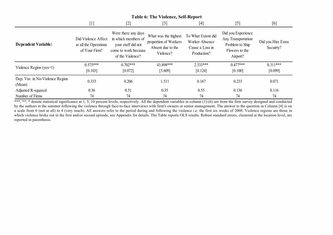
Table 6: The Violence, Self-Report

***, **, * denote statistical significance at 1, 5, 10 percent levels, respectively. All the dependent variables in column (1)-(6) are from the firm survey designed and conducted by the authors in the summer following the violence through face-to-face interviews with firm's owners or senior management. The answer to the question in Column [4] is on a scale from 0 (not at all) to 4 (very much). All answers refer to the period during and following the violence i.e. the first six weeks of 2008. Violence regions are those in which violence broke out in the first and/or second episode, see Appendix for details. The Table reports OLS results. Robust standard errors, clustered at the location level, are reported in parenthesis.

[1] [2] [3] [4] [5] [6]

Dependent Variable:Did Violence Affect at all the Operations

of Your Firm?

Were there any days in which members of

your staff did not come to work because

of the Violence?

What was the highest proportion of Workers

Absent due to the Violence?

To What Extent did Worker Absence Cause a Loss in

Production?

Did you Experience Any Transportation

Problem to Ship Flowers to the

Airport?

Did you Hire Extra Secuirty?

0.575*** 0.702*** 43.898*** 2.333*** 0.477*** 0.311***[0.103] [0.072] [5.609] [0.124] [0.100] [0.099]

Dep. Var. in No-Violence Region (Mean)

0.333 0.206 1.511 0.167 0.233 0.071

Adjusted R-squared 0.36 0.51 0.35 0.55 0.136 0.116Number of Firms 74 74 74 74 74 74

Violence Region (yes=1)

Table 7: Disentangling Channels: Workers Losses versus Transportation Problems

***, **, * denote statistical significance at 1, 5, 10 percent levels, respectively. The sample includes only 74 interviewed firms for which information on workers absent and transportation problems experienced during the six weeks after the beginning of the violence are available. Since this information was collected retrospectively for each separate week, each observation corresponds to a firm in a given week. % Workers Lost is a week level variable for each firm and transportation problem is a dummy which takes value equal to 1 if during a particular week a firm suffered transport issues. The sample period is as in Table 3. Standard errors in ( ) are obtained by multi-way clustering at the firm and location-winter-week level [see Cameron et al, (2009)].

Dependent Variable: Log (1+ weekly exports volumes) [1] [2] [3] [4] [5] [6]-0.414** -0.078 -0.108 -0.091(0.189) (0.153) (0.173) (0.188)

-0.014*** -0.012*** -0.014** -0.014**(0.004) (0.004) (0.006) (0.006)

-0.574** -0.265 -0.117 -0.081(0.263) (0.253) (0.202) (0.108)

0.088(0.518)

-0.299(0.708)

Fixed EffectsFirm * Winter yes yes yes yes yes yesFirm * Week yes yes yes yes yes yesAdjusted R-squared 0.815 0.814 0.815 0.821 0.82 0.82Number of observations 3710 3710 3710 3710 3710 3710

Week of Violence (yes=1) * Violence location (yes=1)

% Workers Absent

Transportation Problems suffered by firm (yes=1)

Week of Violence (yes=1) * Violence location (yes=1) * Only Auction (yes=1)

Week of Violence (yes=1) * Violence location (yes=1) * Small Firm (yes=1)

Table 8: Missing Workers, Survey Evidence

***, **, * denote statistical significance at 1, 5, 10 percent levels, respectively. % of Workers lost is the highest percentage reported by the firm throughout the violence period, i.e., during the first six weeks of 2008. The sample includes all interviewed firms in the violence region. Only auction takes value equal to one if the firm exports more than 90% of production to the auctions. Small firm takes value equal to one if the firm is smaller than the median firm in the industry. Housing offered takes value equal to one if the firm provides housing for more than 20% of the permanent labour force. Only roses takes value equal to one if roses are more than 90% of a firm export volumes. No insulated trucks takes value equal to one for those firms that do not own trucks. Robust standard errors are reported in parenthesis.

Dep. Variable = % Workers Lost (1) (2) (3) (4) (5) (6)23.05 27.27** 29.07** 25.58* 20.24* 27.17*

(15.60) (13.48) (13.47) (14.74) (12.04) (15.49)26.51** 31.86** 25.47* 32.51*** 7.82 33.66**(11.45) (12.33) (15.40) (12.46) (11.22) (15.08)

-16.87* -20.1* -14.137 -27.31** -17.52(10.07) (10.33) (10.83) (10.26) (10.85)

-16.50(12.73)-3.123(17.25)

-19.085(13.41)

-17.527(11.73)

0.383(0.269)0.341

(0.278)0.673

(11.46)-4.015(14.32)

Fixed Effects location (4) location (4) location (4) location (4) location (4) location (4)Observations (firms) 44 44 44 44 44 44Pseudo R-squared 0.282 0.352 0.401 0.394 0.584 0.354

Only Auction (yes=1)

Only Roses (yes=1)

No Insulated Trucks (yes=1)

Small Firm (yes=1)

% of Female Workers

% of Workers with Primary Education

Housing Offered (yes=1)

KFC Member (yes=1)

Fair Trade Certification (yes=1)

Politically connected firm (yes=1)

Foreign Owner (yes=1)

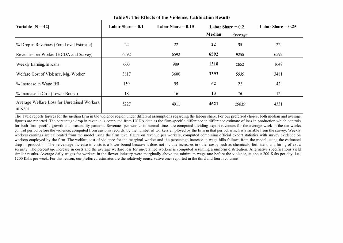
Table 9: The Effects of the Violence, Calibration Results

The Table reports figures for the median firm in the violence region under different assumptions regarding the labour share. For our preferred choice, both median and average figures are reported. The percentage drop in revenue is computed from HCDA data as the firm-specific difference in difference estimate of loss in production which controls for both firm-specific growth and seasonality patterns. Revenues per worker in normal times are computed dividing export revenues for the average week in the ten weeks control period before the violence, computed from customs records, by the number of workers employed by the firm in that period, which is available from the survey. Weekly workers earnings are calibrated from the model using the firm level figure on revenue per workers, computed combining official export statistics with survey evidence on workers employed by the firm. The welfare cost of violence for the marginal worker and the percentage increase in wage bills follows from the model, using the estimated drop in production. The percentage increase in costs is a lower bound because it does not include increases in other costs, such as chemicals, fertilizers, and hiring of extra security. The percentage increase in costs and the average welfare loss for un-retained workers is computed assuming a uniform distribution. Alternative specifications yield similar results. Average daily wages for workers in the flower industry were marginally above the minimum wage rate before the violence, at about 200 Kshs per day, i.e., 1200 Kshs per week. For this reason, our preferred estimates are the relatively conservative ones reported in the third and fourth columns

Variable [N = 42] Labor Share = 0.1 Labor Share = 0.15 Labor Share = 0.25

Median Average

% Drop in Revenues (Firm Level Estimate) 22 22 22 38 22

Revenues per Worker (HCDA and Survey) 6592 6592 6592 9258 6592

Weekly Earning, in Kshs 660 989 1318 1851 1648

Welfare Cost of Violence, Mg. Worker 3817 3600 3393 5939 3481

% Increase in Wage Bill 159 95 62 71 42

% Increase in Cost (Lower Bound) 18 16 13 16 12

Average Welfare Loss for Unretained Workers, in Kshs

5227 4911 4621 19819 4331

Labor Share = 0.2

Table A1: Electoral Violence in Sub-Saharan Africa

The Tables updates the records in Straus and Taylor (2009). Straus and Taylor (2009) study 213 elections (presidential and parliamentary) in 45 African countries during the period 1990-2007. Electoral violence is defined as those elections that feature repression, a violent campaign, and incidents leading to 20 or more deaths. Sources: Lindberg (2006), Straus and Taylor (2009) and UN General Assembly – Election-related violence and killings (2010).

Country Year Characteristics of Violence (Examples)

Mauritania 1992Comoros 1992Angola 1992Cen. Africa Rep. 1992Kenya 1992, 1997, 2007 Election fraud [2 months, 1,113 + dead]Nigeria 1992, 1993, 1999, 2007 State sponsored violence against opposition [200+ dead]Senegal 1993Togo 1993, 1994, 1998, 2003, 2005 State sponsored violence against opposition [700+ dead, 40,000+ fled to nearby country]EQ Guinea 1993, 1996, 1999, 2004Guinea 1993, 1998, 2010 Opposition protest over military junta [1 day, 156 dead]DR Congo 1993, 2006 Opposition reject run-off results [3 weeks +, 200+ dead]South Africa 1994, 1999Cote d'Ivoire 1995, 2000, 2010 Postponing of presidential elections [1 day, 5 dead, 10+ wounded]Sudan 1996, 2000Niger 1996Lesotho 1998Nigeria 1999, 2003, 2007 State sponsored violence against opposition [200+ dead]Tanzania 2000Zimbabwe 2000, 2002, 2005, 2008 State sponsored violence against opposition [180+ dead, 1000+ abductions, tortures etc]Ethiopia 2000, 2005 Demonstration by opposition against electoral fraud [1 day, 36 dead, 100+ wounded]Madagascar 2001, 2009 Anti-government protests by opposition [9 months, 135+ dead]Burundi 2005

Table A2: Location of Firms and Definition of Violence

Notes: First Outbreak of Violence: 29 Dec 2007 - 4 Jan 2008. Second Outbreak of Violence: 25 Jan 2008 - 30 Jan 2008. Total No. of firms 104.

Table A3: Calendar of Events

First Outbreak of Violence:

Second Outbreak of Violence:

Violence =1, No-conflict=0

Violence =1, No-conflict=0

Central Kiambu (2) 0 0Central Kikuyu (1) 0 0Central Limuru (10) 0 1Central Nyeri (2) 0 0Central Thika (19) 0 0Eastern Athi River (10) 0 0Eastern Timau (3) 0 0Nairobi Nairobi (5) 0 0

Rift Valley Elburgon (1) 1 1Rift Valley Eldoret (4) 1 1Rift Valley Kericho (1) 1 1Rift Valley Kitale (2) 1 1Rift Valley Naivasha (25) 0 1Rift Valley Nakuru (10) 1 1Rift Valley Nanyuki (5) 0 0Rift Valley Nyahururu (4) 0 0

ProvinceTown (No. of

Firms)

Sunday Monday Tuesday Wednesday Thursday Friday Saturday

23 24 25 2627

ELECTION DAY28

29 First Outbreak of

Violence

30 Elections Results

announced 31

1 2 3 4 5

6 7 8 9 10 11 12

13 14 15 16 17 18 19

20 21 22 23 24

25 Second Outbreak

of Violence as mediation efforts

fail.

26

27 28 29 30 31

1 2

3 4 5 6 7 8 9

……………28

Power Sharing Agreement

DEC

EMBE

RJA

NU

AR

YFE

BRU

AR

Y

Table A4: Placebos -- No Differential Seasonality Across Regions

***, **, * denote statistically significance at 1, 5, 10 percent, respectively. Columns (a) and (b) report means of average daily export weight (in log kgs) in rows 1-2(c) (standard deviation are reported in parenthesis). Column (c) reports the corresponding difference, with standard errors in ( ) clustered at the firm level. In Panel A: Violence region is defined as the locations which suffered violence during the first outbreak. These locations are the towns of Eldoret, Kitale, Elburgon, Kericho and Nakuru. In Panel B: Violence region is defined as the locations which suffered violence during the first and second outbreak. These locations are the towns of Eldoret, Kitale, Elburgon, Kericho, Nakuru, Naivasha and Limuru, see Table A1 for details.

Non-Violence Region

Violence RegionViolence - Non-Violence

Difference

5.844 6.744 0.899[2.722] [1.986] (0.554)

6.154 6.81 0.656[2.269] [2.07] (0.544)

6.03 5.95 -0.082[2.226] [2.682] (0.730)

6.398 6.598 0.2[1.794] [2.145] (0.585)

-0.309* -0.066 0.243(0.168) (0.484) (0.499)

-0.187 0.794 0.981(0.321) (0.691) (0.744)

0.057 0.64 Triple Difference(0.292) (0.767) 0.583

(0.801)

Non-Violence Region

Violence RegionViolence - Non-Violence

Difference6.379 6.271 -0.109

[2.267] [2.287] (0.466)

6.368 6.196 -0.172[2.17] [2.310] (0.458)

6.775 6.696 -0.079[1.724] [1.920] (0.402)

6.532 6.346 -0.186[1.682] [2.006] (0.408)

0.011 0.074 0.063(0.211) (0.280) (0.350)

-0.395 -0.4255 -0.0301(0.350) (0.364) (0.503)

-0.044 -0.181 Triple Difference(0.298) (0.412) -0.137

(0.506)

3a

First Differences

[1]-[2a]

3b [1]-[2b]

4Regional Difference in

Difference([1]-[2a]) - ([2b]-[2c])

2a

Control Periods

Winter -1: Control Period [4 Nov 2005 - 22 Dec 2005]

2b Winter -2: Violence Period [25 Jan 2005 - 30 Jan 2005]

2c Winter -2: Control Period [4 Nov 2004 - 22 Dec 2004]

4Regional Difference in

Difference([1]-[2a]) - ([2b]-[2c])

1 Treatment PeriodWinter -1: Violence Period [25 Jan

2006 - 30 Jan 2006]

Panel B: Regions of Violence are location which suffered in the second outbreak of Violence

3a

First Differences

[1]-[2a]

3b [1]-[2b]

1 Treatment PeriodWinter -1:Violence Period [29 Dec

2005 - 4 Jan 2006]

Panel A: Regions of Violence are locations which suffered in the first outbreak of Violence

2a

Control Periods

Winter -1: Control Period [4 Nov 2006 - 22 Dec 2006]

2b Winter -2: Violence Period [29 Dec 2004 - 4 Jan 2005]

2c Winter -2: Control Period [4 Nov 2004 - 22 Dec 2004]

Figure 1: Effect of Violence on Export Volumes

Notes: The figure shows the median biweekly residual of a regression that controls for firm specific seasonality and growth patterns in violence and in no-violence locations for the 10 weeks before and 10 weeks after the first outbreak of violence.

Figure 2: Effect of Violence on Export Volumes

Notes: The figure shows the estimated coefficients of the differential cumulative and medium-run effects of the violence following the second outbreak using the baseline specification in Column IV of Table 3.

-6-4

-20

2

De-

Seas

onal

ized

Vol

umes

(Log

)

-10 -5 0 5 10Weeks from Beginning of Conflict

Conflict No ConflictDifference

-.6-.4

-.20

.2

Est

imat

ed C

oeffi

cien

ts

0 10 20 30

Days after End of 2nd Spike of Violence

Cumulative Treatment Effect

Post-Treatment Effect

Cumulative and Medium Run Effects of the Violence

Figure A1: Flower Firms Location and Violence Regions

Notes: the figure displays the geographical distribution of the nearest towns to the flower farms as well as whether the relevant locations had been involved in either the first or the second outburst of violence.

Documents

Guns and Roses: Flower Exports and Electoral Violence in Kenya