1

������������������������������ ���� ��������������� ���� ��������������� ���� ��������������� ���� ���������

����������������������� �!"#�����$����������������������� �!"#�����$����������������������� �!"#�����$����������������������� �!"#�����$����

I.Gultepe1, R. Rasmussen2, B. Zhou3, R. K. Ungar4, and R. Nitu5

1Cloud Physics and Severe Weather Research Section, Science and Technology Branch, Environment Canada, Toronto, Ontario M3H 5T4

2National Center for Atmospheric Research, PO Box 3000, Boulder, CO 80307

3Environmental Modeling Center, NCEP/NOAA, 5200 Auth Rd, Camp Springs, MD 20746

4Verification and Incident Monitoring Radiation Protection Bureau, 775 Brookfield Road, AL6302D1, Ottawa, Ontario K1A 1C1

5Atmospheric Monitoring and Water Survey Directorate, Environment Canada, Toronto, Ont. M3H5T4

ABSTRACT

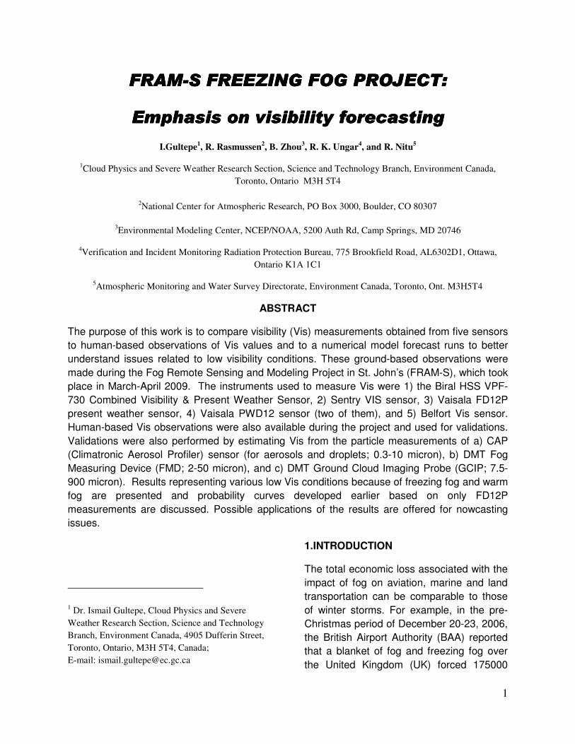
The purpose of this work is to compare visibility (Vis) measurements obtained from five sensors to human-based observations of Vis values and to a numerical model forecast runs to better understand issues related to low visibility conditions. These ground-based observations were made during the Fog Remote Sensing and Modeling Project in St. John’s (FRAM-S), which took place in March-April 2009. The instruments used to measure Vis were 1) the Biral HSS VPF-730 Combined Visibility & Present Weather Sensor, 2) Sentry VIS sensor, 3) Vaisala FD12P present weather sensor, 4) Vaisala PWD12 sensor (two of them), and 5) Belfort Vis sensor. Human-based Vis observations were also available during the project and used for validations. Validations were also performed by estimating Vis from the particle measurements of a) CAP (Climatronic Aerosol Profiler) sensor (for aerosols and droplets; 0.3-10 micron), b) DMT Fog Measuring Device (FMD; 2-50 micron), and c) DMT Ground Cloud Imaging Probe (GCIP; 7.5-900 micron). Results representing various low Vis conditions because of freezing fog and warm fog are presented and probability curves developed earlier based on only FD12P measurements are discussed. Possible applications of the results are offered for nowcasting issues.

1

1 Dr. Ismail Gultepe, Cloud Physics and Severe Weather Research Section, Science and Technology Branch, Environment Canada, 4905 Dufferin Street, Toronto, Ontario, M3H 5T4, Canada; E-mail: ismail.gultepe@ec.gc.ca

1.INTRODUCTION

The total economic loss associated with the impact of fog on aviation, marine and land transportation can be comparable to those of winter storms. For example, in the pre-Christmas period of December 20-23, 2006, the British Airport Authority (BAA) reported that a blanket of fog and freezing fog over the United Kingdom (UK) forced 175000

2

passengers to miss flights from its seven British airports, with Heathrow the worst affected (Milmo, 2007). Early estimates suggested this disruption to air travel cost British Airways at least £25 million (Gadher and Baird, 2007). The costs to stranded passengers in terms of money and inconvenience may be impossible to calculate. Previous studies have also shown that human and financial losses due to accidents related to fog episodes were very common. In Canada, approximately 50 people per year die due to fog related motor vehicle accidents (Gultepe et al., 2009).

The purpose of this work is to compare a) visibility measurements (Vis) obtained from the five Vis sensors to human-based observations of Vis to better understand issues related to low visibility conditions and b) compare the results to those obtained from the US NAM (North American Mesoscale) model runs for two cases: 1) freezing fog event (March 25-27 2009, Fig. 1a) and 2) warm fog event (April 5-7 2009, Fig. 1b).

2.OBSERVATIONS

The ground-based observations from the Fog Remote Sensing and Modeling Project in St. John’s (FRAM-S), which took place at St. John’s International Airport, NFL, Canada, in March-April 2009, were used in the analysis.

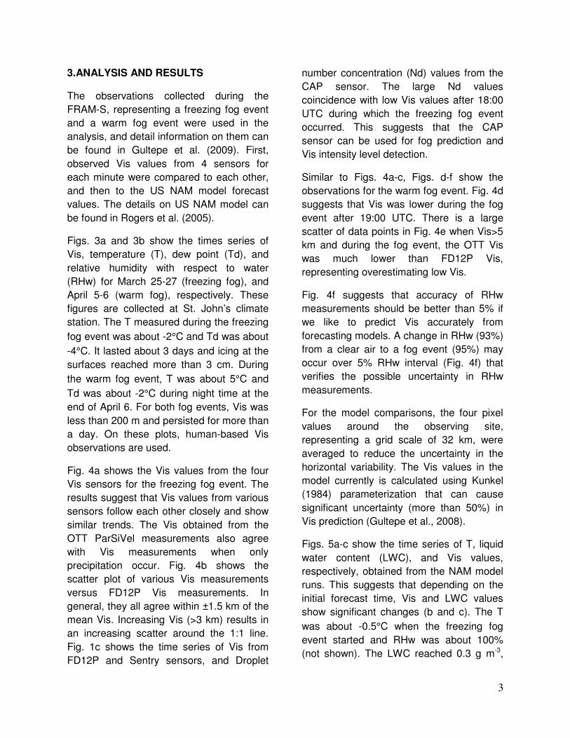
The instruments used to measure Vis were 1) the Biral HSS VPF-730 Combined Visibility & Present Weather Sensor (Fig. 1c), 2) Sentry VIS sensor (Fig. 1d), 3) Vaisala PWD12 sensor (Fig. 1e), 4) Vaisala FD12P present weather sensor (Fig. 1f), and 5) Belfort Vis sensor (Fig. 1g). All of these sensors use a visible light source to estimate extinction of light in a small

sampling volume between their transmitting and receiving arms. Human-based Vis observations were also available during the project. In the analysis, the measurements of Vis were compared to human-based Vis observations and to each other.

The particle measurements from a) CAP aerosol sensor (for aerosols and droplets; 0.3-10 micron, Gultepe et al., 2009), b) DMT Fog Measuring Device (FMD; 2-50 micron), and c) DMT Ground Cloud Imaging Probe (GCIP; 7.5-900 micron) were also made. The Fig. 2 shows the GCIP configuration in the field (a) and an example of warm fog/drizzle images (b), and mixed phase conditions with small droplets, wet snow, and columnar ice crystals (c). In the images, the smallest size is about 10 micron and the largest one is about 900 micron.

The NCEP NAM Model is a major operational regional model routinely used by NWS WFO forecasters over entire US. The NAM has four cycle runs (00Z, 06Z, 12Z, and 18Z) per day with every one or every three hour output out to 87 forecast hours. Before 36 forecast hours, it has output every one hour, and after 36 hours, it has output every three hours. The model physics can be found in Janji� (1994), Ferrier (2002), Janjic (1994), Janjic and Janjic (1996), Schwarzkopf and Fels (1991), and Ek et al. (2003). The NAM-12 km output are projected on different grid resolution format outputs, including 12 km (grid#218), 32 km (grid#221), 40 km (grid#212), and 90 km (grid#104), etc. For St. John’s FRAM-S project, the grid#221 (32 km) is used. The 60 levels in the vertical were used and the lowest resolution was about 30 m.

3

3.ANALYSIS AND RESULTS

The observations collected during the FRAM-S, representing a freezing fog event and a warm fog event were used in the analysis, and detail information on them can be found in Gultepe et al. (2009). First, observed Vis values from 4 sensors for each minute were compared to each other, and then to the US NAM model forecast values. The details on US NAM model can be found in Rogers et al. (2005).

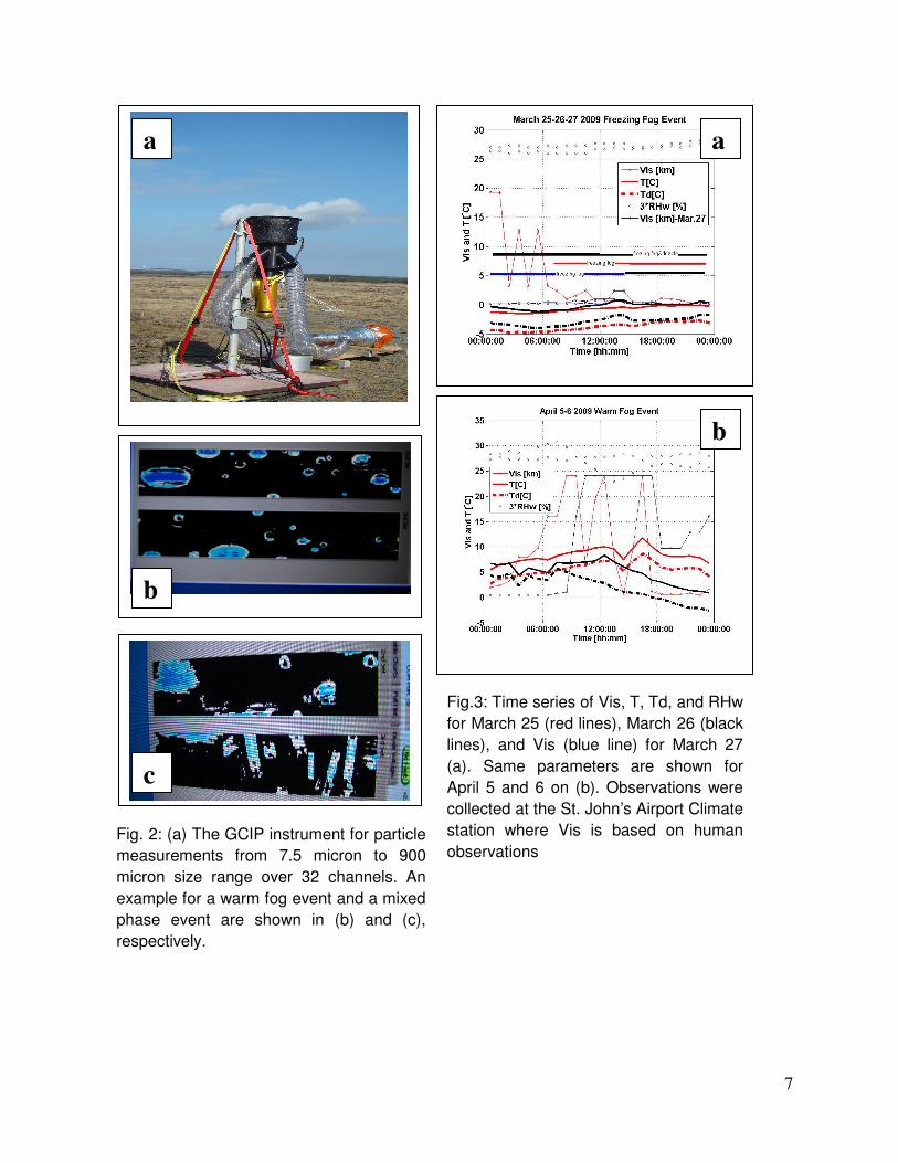
Figs. 3a and 3b show the times series of Vis, temperature (T), dew point (Td), and relative humidity with respect to water (RHw) for March 25-27 (freezing fog), and April 5-6 (warm fog), respectively. These figures are collected at St. John’s climate station. The T measured during the freezing fog event was about -2°C and Td was about -4°C. It lasted about 3 days and icing at the surfaces reached more than 3 cm. During the warm fog event, T was about 5°C and Td was about -2°C during night time at the end of April 6. For both fog events, Vis was less than 200 m and persisted for more than a day. On these plots, human-based Vis observations are used.

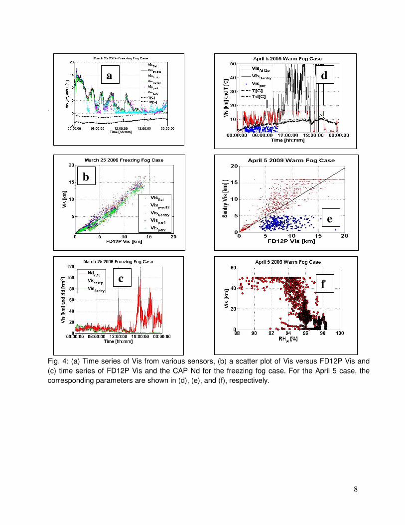
Fig. 4a shows the Vis values from the four Vis sensors for the freezing fog event. The results suggest that Vis values from various sensors follow each other closely and show similar trends. The Vis obtained from the OTT ParSiVel measurements also agree with Vis measurements when only precipitation occur. Fig. 4b shows the scatter plot of various Vis measurements versus FD12P Vis measurements. In general, they all agree within ±1.5 km of the mean Vis. Increasing Vis (>3 km) results in an increasing scatter around the 1:1 line. Fig. 1c shows the time series of Vis from FD12P and Sentry sensors, and Droplet

number concentration (Nd) values from the CAP sensor. The large Nd values coincidence with low Vis values after 18:00 UTC during which the freezing fog event occurred. This suggests that the CAP sensor can be used for fog prediction and Vis intensity level detection.

Similar to Figs. 4a-c, Figs. d-f show the observations for the warm fog event. Fig. 4d suggests that Vis was lower during the fog event after 19:00 UTC. There is a large scatter of data points in Fig. 4e when Vis>5 km and during the fog event, the OTT Vis was much lower than FD12P Vis, representing overestimating low Vis.

Fig. 4f suggests that accuracy of RHw measurements should be better than 5% if we like to predict Vis accurately from forecasting models. A change in RHw (93%) from a clear air to a fog event (95%) may occur over 5% RHw interval (Fig. 4f) that verifies the possible uncertainty in RHw measurements.

For the model comparisons, the four pixel values around the observing site, representing a grid scale of 32 km, were averaged to reduce the uncertainty in the horizontal variability. The Vis values in the model currently is calculated using Kunkel (1984) parameterization that can cause significant uncertainty (more than 50%) in Vis prediction (Gultepe et al., 2008).

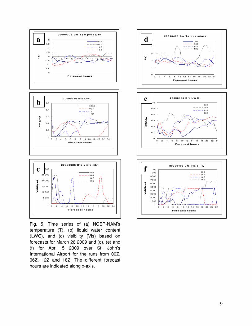
Figs. 5a-c show the time series of T, liquid water content (LWC), and Vis values, respectively, obtained from the NAM model runs. This suggests that depending on the initial forecast time, Vis and LWC values show significant changes (b and c). The T was about -0.5°C when the freezing fog event started and RHw was about 100% (not shown). The LWC reached 0.3 g m-3,

4

comparable to previous LWC measurements (Gultepe et al., 2009).

Figs. 5d-f show the measurements for the warm fog event. During the fog event, the LWC values were greater than the cold fog case and T was about 2°C lower than observations (Fig. 4d). The Vis values were comparable with those of human-based observations (Fig. 4d).

Comparisons between human-based observations (Fig. 3) and sensor-based Vis values (fig. 4) suggest that Vis sensor values were usually close to the human-based Vis values but note that variability in fog and its Vis over the area can be an important source of error, and this will be analyzed in more detail in the future.

4.DISCUSSION AND CONCLUSION

Observations collected during the FRAM-S project are being used currently for Vis analysis during the two fog events. Preliminary results suggest that uncertainty in the measurements of Vis can be as high 4-5 km in the higher Vis values to 1 km in the lower Vis values. Difference among the Vis based on various sensors can also be significant especially during the precipitation events.

Model based Vis values strongly depend on:

a) Accuracy of RHw.

b) Accuracy of LWC or ice water content (IWC).

c) Accuracy of precipitation amounts and types.

d) Model run times and its horizontal and vertical time and space resolutions.

e) Fog-cloud microphysical processes.

Improvement of prediction of the above parameters can significantly improve Vis prediction for the various fog conditions. One example shown here suggested that accuracy of RHw should be better than 5% (Fig. 4f) which is not feasible currently from either measurements or models. Other parameters significantly affecting the Vis from the models are LWC and Nd that should be used in fog Vis predictions and using only LWC can cause more than 50% uncertainty in model-based Vis (Gultepe et al 2009).

Freezing fog events are very common during the winter (Gultepe et al., 2009) over the northern maritime regions. During the FRAM-S project, we had at least 2 major events and these observations will be analyzed in more detail in the future. The FMD measurements will also be used to develop a freezing fog parameterization and tested using a forecasting model. This work is currently in progress.

Probabilistic approaches for visibility prediction (Gultepe et al., 2009) can be very useful when accuracy of model-based parameters includes large uncertainties. The relationships representing mean curve fits cannot be accurate enough to be used in model simulations because of the weakness of the relationship between Vis and precipitation amounts. Parameterizations can be even worse when the snow type is not known (Rasmussen et al, 1999).

5

5.REFERENCES

Ek, M. B., K. E. Mitchell, Y. Lin, E. Rogers, P. Grunmann, V. Koren, G. Gayno, and J.D. Tarpley, 2003: Implementation of Noah land surface model advances in the National Centers for Environmental Prediction operational mesoscale Eta model, J. Geophys. Res. 108(D22), 8851.

Ferrier B. S., 2002: A new grid-scale cloud and precipitation scheme in the NCEP Eta model. Technical report, Spring Colloquium on the Physics of Weather and Climate: Regional weather prediction modeling and predictability.

Gadher, D, and Baird, T, cited 2007: Airport dash as the fog lifts, The Sunday Times, posted online 24 December 2006. At http://www.timesonline.co.uk/article/0,,2087-2517675.html.]

Gultepe, I., R. Tardif, S.C. Michaelides, J.Cermak, A. Bott, J. Bendix, M. Müller, M. Pagowski, B. Hansen, G. Ellrod, W. Jacobs, G. Toth, S.G. Cober, 2007: Fog research: a review of past achievements and future perspectives. J. of Pure and Applied Geophy., Special issue on fog, edited by I. Gultepe. 164, 1121-1159.

Gultepe, I., G. Pearson J. A. Milbrandt, B. Hansen, S. Platnick, P. Taylor, M. Gordon, J. P. Oakley, 2009, and S.G. Cober: The fog remote sensing and modeling (FRAM) field project. Bull. Of Amer. Meteor. Soc., 90, 341-359.

Gultepe, I., M. D. Müller, and Z. Boybeyi, 2006: A new visibility parameterization for warm fog applications in numerical weather prediction models. J. Appl. Meteor., 45, 1469-1480.

Janji�, Z. I., 1994: The step-mountain eta coordinate model: Further developments of the convection, viscous sublayer, and turbulence closure schemes. Mon. Wea. Rev., 124, 1225-1242.

Janji�, Z. I., 1996: The Surface Layer in the NCEP Eta Model. Reprints, 11th Conf. on NWP, Norfolk, VA, Amer. Meteor. Soc., 354-355.

Kunkel, B. A., 1984: Parameterization of droplet terminal velocity and extinction coefficient in fog models. J. Appl. Meteor., 23, 34-41.

Milmo, D., 2007: BAA counts the cost of December fog, Guardian Unlimited, At http://www.guardian.co.uk/airlines/story/0,,1986427,00.html on 9 Jan. 2007.

Rasmussen, R. M., J. Vivekanandan, J. Cole, B. Myers, and C. Masters, 1999: The estimation of snowfall rate using visibility. J. Applied. Meteor., 38, 1542-1563.

Rogers, E., Y. Lin, K. Mitchell, W.-S. Wu, B. Ferrier, G. Gayno, M. Pondeca, M. Pyle, V. Wong, and M. Ek, 2005: The NCEP North American Modeling System: Final Eta model analysis changes and preliminary experiments using the WRF-NMM. Proc. 21st Conference on Weather Analysis and Forecasting/17th Conference on Numerical Weather Prediction, American Meteorological Society, Washington, DC.

Schwarzkopf, M. D., and S. B. Fels, 1991: The simplified exchange method revisited: An accurate, rapid method for computation of infrared cooling rats and fluxes. J. Geophys. Res., 96, 9075-9096.

Acknowledgment

Funding for the FRAM-S project was provided by the Canadian National Search and Rescue (SAR) Secretariat and Environment Canada (EC). The authors are thankful to M. Wasey, K. Wu, and R. Reed of Environment Canada for technical support.

6

Fig. 1: (a) The freezing fog event on March 25 2009 and (b) warm fog event on April 5 2009. The HSS, Sentry, PWD12, FD12P, and Belfort Vis sensors are shown in (c), (d), (e), (f), and (g), respectively.

a

f c

b e

d

g

7

.

a

b

c

a

b

Fig.3: Time series of Vis, T, Td, and RHw for March 25 (red lines), March 26 (black lines), and Vis (blue line) for March 27 (a). Same parameters are shown for April 5 and 6 on (b). Observations were collected at the St. John’s Airport Climate station where Vis is based on human observations

Fig. 2: (a) The GCIP instrument for particle measurements from 7.5 micron to 900 micron size range over 32 channels. An example for a warm fog event and a mixed phase event are shown in (b) and (c), respectively.

8

,

Fig. 4: (a) Time series of Vis from various sensors, (b) a scatter plot of Vis versus FD12P Vis and (c) time series of FD12P Vis and the CAP Nd for the freezing fog case. For the April 5 case, the corresponding parameters are shown in (d), (e), and (f), respectively.

a

b

c

d

e

f

9

Fig. 5: Time series of (a) NCEP-NAM’s temperature (T), (b) liquid water content (LWC), and (c) visibility (Vis) based on forecasts for March 26 2009 and (d), (e) and (f) for April 5 2009 over St. John’s International Airport for the runs from 00Z, 06Z, 12Z and 18Z. The different forecast hours are indicated along x-axis.

20090405 S fc V isib i li ty

0

1000

2000

3000

4000

5000

6000

7000

8000

9000

10000

0 2 4 6 8 10 12 14 16 18 20 22 24

Fore ca st h ours

Vis

ibili

ty (m

)

00Z

06Z12Z18Z

20090405 2m Te m pe ra ture

0

1

2

3

4

5

0 2 4 6 8 10 12 14 16 18 20 22 24

F o re ca st ho u rs

T (C

)

00Z06Z12Z18Z

20090405 S fc L W C

0

0.1

0.2

0.3

0.4

0.5

0.6

0 2 4 6 8 10 12 14 16 18 20 22 24

F ore ca st h ou rsLW

C (g

/kg)

00Z

06Z

12Z

18Z

20090326 2m Te m pe ra tu re

-2

-1 .5

-1

-0 .5

0

0.5

1

1.5

2

0 2 4 6 8 10 12 14 16 18 20 22 24

F o re ca st h o urs

T (C

)00Z

06Z

12Z

18Z

20090326 S fc V isib i l ity

0

5000

10000

15000

20000

25000

30000

0 2 4 6 8 10 12 14 16 18 20 22 24

Fore ca st hours

Vis

ibili

ty (m

)

00Z

06Z

12Z

18Z

20090326 S fc L W C

0

0.1

0.2

0.3

0.4

0.5

0 2 4 6 8 10 12 14 16 18 20 22 24

F o re ca st h o u rs

LWC (g

/kg)

006Z

06Z

12Z18Z

a

b

c

d

e

f