Training in Task Space to Speed Up and Guide Reinforcement Learning

Guillaume Bellegarda and Katie Byl

Abstract— Recent breakthroughs in the reinforcement learn-ing (RL) community have made significant advances towardslearning and deploying policies on real world robotic systems.However, even with the current state-of-the-art algorithms andcomputational resources, these algorithms are still plaguedwith high sample complexity, and thus long training times,especially for high degree of freedom (DOF) systems. Thereare also concerns arising from lack of perceived stability orrobustness guarantees from emerging policies. This paper aimsat mitigating these drawbacks by: (1) modeling a complex,high DOF system with a representative simple one, (2) makingexplicit use of forward and inverse kinematics without forcingthe RL algorithm to “learn” them on its own, and (3) learninglocomotion policies in Cartesian space instead of joint space.In this paper these methods are applied to JPL’s Robosimian,but can be readily used on any system with a base and endeffector(s). These locomotion policies can be produced in justa few minutes, trained on a single laptop. We compare therobustness of the resulting learned policies to those of othercontrol methods. An accompanying video for this paper can befound at https://youtu.be/xDxxSw5ahnc.

I. INTRODUCTION

Without loss of generality to other systems with end effec-tors, this work aims specifically at increasing robustness andstability of skating motions designed for JPL’s Robosimianquadruped [1], [2], [3], [4], [5], which is shown in Figure 1.Previous work in [6] describes an overview of hand-designedskating motions on passive unactuated wheels mounted ateach forearm of Robosimian’s four identical limbs, com-paring specifically skating with three vs. four wheels incontact with the ground. Results showed that on flat ground,skating on four wheels demonstrated greater robustness dueto symmetry and thus decreased wheel slip. However onterrain with bumps or other curvature, the asymmetry inconfiguration and contact force distribution over time fromskating on three wheels had the advantage of guaranteeingcontinuous ground contact for all skates. It is clear in eithercase that such hand-designed open-loop trajectories leavemuch to be desired in terms of robustness to disturbancesand noise in the environment. We would like guarantees onperformance, and ideally to have some confidence estimateon performance/time to complete a task in a new scenario.

This lack of robustness, combined with impressive recentresults applying reinforcement learning algorithms such asProximal Policy Optimization (PPO) [8] [9], Trust Re-gion Policy Optimization (TRPO) [10], Actor Critic us-ing Kronecker-Factored Trust Region (ACKTR) [11], Deep

This work was funded in part by NSF NRI award 1526424.Guillaume Bellegarda and Katie Byl are with the Robotics Labora-

tory, Department of Electrical and Computer Engineering, University ofCalifornia at Santa Barbara (UCSB). gbellegarda@ucsb.edu,katiebyl@ucsb.edu

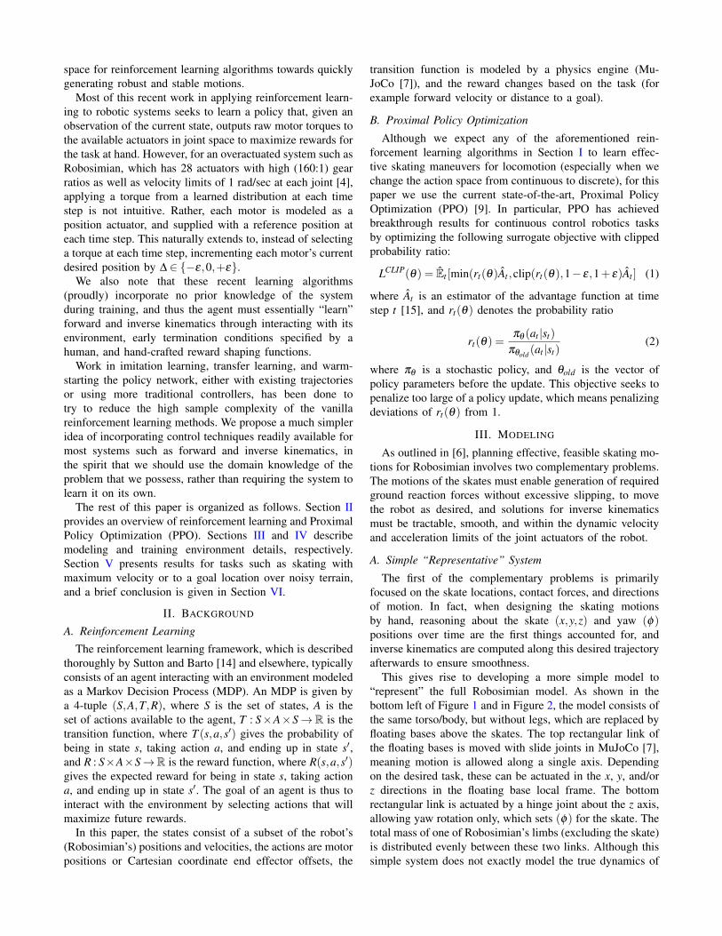
Fig. 1. Versatile Locomotion with Robosimian. Top: Skating on flatground with the real system. Bottom: Simple Cartesian space model andfull Robosimian model, in MuJoCo [7].

Deterministic Policy Gradients (DDPG) [12], and Asyn-chronous Advantage Actor-Critic (A3C) [13], to continuouscontrol tasks in robotics, suggests the use of (deep) rein-forcement learning as a way to increase skating stability androbustness. However, as powerful and promising as theserecent results have been, the sample complexity and trainingtime of these methods remains a major issue when seekingto deploy solutions in real time in the real world. Even forstate-of-the-art algorithms and implementations, especiallyfor high degree of freedom (DOF) complex systems such asRobosimian, a policy can take millions of iterations to trainfor a solution that may or may not be stable. It must also benoted that there are no robustness, stability, or performanceguarantees on the policies learned, or at least no way toreadily quantify these metrics.

One prominent example is shown in the video associatedwith Heess et. al’s Emergence of Locomotion Behaviours inRich Environments [8], where for the higher DOF systemhumanoid, we see the emergence of (probably) non-optimaland non-intuitive arm-flailing to “help” locomote the system,as a probable local optimum. The video accompanyingthe present paper shows an example of the emergence ofsimilar non-intuitive behavior when learning a locomotionpolicy with PPO [9] for Robosimian in joint space. Weseek to avoid such local optima for locomotion policiesin our system, and propose intuitively limiting the action

arX

iv:1

903.

0221

9v1

[cs

.RO

] 6

Mar

201

9

space for reinforcement learning algorithms towards quicklygenerating robust and stable motions.

Most of this recent work in applying reinforcement learn-ing to robotic systems seeks to learn a policy that, given anobservation of the current state, outputs raw motor torques tothe available actuators in joint space to maximize rewards forthe task at hand. However, for an overactuated system such asRobosimian, which has 28 actuators with high (160:1) gearratios as well as velocity limits of 1 rad/sec at each joint [4],applying a torque from a learned distribution at each timestep is not intuitive. Rather, each motor is modeled as aposition actuator, and supplied with a reference position ateach time step. This naturally extends to, instead of selectinga torque at each time step, incrementing each motor’s currentdesired position by ∆ ∈ {−ε,0,+ε}.

We also note that these recent learning algorithms(proudly) incorporate no prior knowledge of the systemduring training, and thus the agent must essentially “learn”forward and inverse kinematics through interacting with itsenvironment, early termination conditions specified by ahuman, and hand-crafted reward shaping functions.

Work in imitation learning, transfer learning, and warm-starting the policy network, either with existing trajectoriesor using more traditional controllers, has been done totry to reduce the high sample complexity of the vanillareinforcement learning methods. We propose a much simpleridea of incorporating control techniques readily available formost systems such as forward and inverse kinematics, inthe spirit that we should use the domain knowledge of theproblem that we possess, rather than requiring the system tolearn it on its own.

The rest of this paper is organized as follows. Section IIprovides an overview of reinforcement learning and ProximalPolicy Optimization (PPO). Sections III and IV describemodeling and training environment details, respectively.Section V presents results for tasks such as skating withmaximum velocity or to a goal location over noisy terrain,and a brief conclusion is given in Section VI.

II. BACKGROUND

A. Reinforcement Learning

The reinforcement learning framework, which is describedthoroughly by Sutton and Barto [14] and elsewhere, typicallyconsists of an agent interacting with an environment modeledas a Markov Decision Process (MDP). An MDP is given bya 4-tuple (S,A,T,R), where S is the set of states, A is theset of actions available to the agent, T : S×A×S→R is thetransition function, where T (s,a,s′) gives the probability ofbeing in state s, taking action a, and ending up in state s′,and R : S×A×S→R is the reward function, where R(s,a,s′)gives the expected reward for being in state s, taking actiona, and ending up in state s′. The goal of an agent is thus tointeract with the environment by selecting actions that willmaximize future rewards.

In this paper, the states consist of a subset of the robot’s(Robosimian’s) positions and velocities, the actions are motorpositions or Cartesian coordinate end effector offsets, the

transition function is modeled by a physics engine (Mu-JoCo [7]), and the reward changes based on the task (forexample forward velocity or distance to a goal).

B. Proximal Policy Optimization

Although we expect any of the aforementioned rein-forcement learning algorithms in Section I to learn effec-tive skating maneuvers for locomotion (especially when wechange the action space from continuous to discrete), for thispaper we use the current state-of-the-art, Proximal PolicyOptimization (PPO) [9]. In particular, PPO has achievedbreakthrough results for continuous control robotics tasksby optimizing the following surrogate objective with clippedprobability ratio:

LCLIP(θ) = Et [min(rt(θ)At ,clip(rt(θ),1− ε,1+ ε)At ] (1)

where At is an estimator of the advantage function at timestep t [15], and rt(θ) denotes the probability ratio

rt(θ) =πθ (at |st)

πθold (at |st)(2)

where πθ is a stochastic policy, and θold is the vector ofpolicy parameters before the update. This objective seeks topenalize too large of a policy update, which means penalizingdeviations of rt(θ) from 1.

III. MODELING

As outlined in [6], planning effective, feasible skating mo-tions for Robosimian involves two complementary problems.The motions of the skates must enable generation of requiredground reaction forces without excessive slipping, to movethe robot as desired, and solutions for inverse kinematicsmust be tractable, smooth, and within the dynamic velocityand acceleration limits of the joint actuators of the robot.

A. Simple “Representative” System

The first of the complementary problems is primarilyfocused on the skate locations, contact forces, and directionsof motion. In fact, when designing the skating motionsby hand, reasoning about the skate (x,y,z) and yaw (φ)positions over time are the first things accounted for, andinverse kinematics are computed along this desired trajectoryafterwards to ensure smoothness.

This gives rise to developing a more simple model to“represent” the full Robosimian model. As shown in thebottom left of Figure 1 and in Figure 2, the model consists ofthe same torso/body, but without legs, which are replaced byfloating bases above the skates. The top rectangular link ofthe floating bases is moved with slide joints in MuJoCo [7],meaning motion is allowed along a single axis. Dependingon the desired task, these can be actuated in the x, y, and/orz directions in the floating base local frame. The bottomrectangular link is actuated by a hinge joint about the z axis,allowing yaw rotation only, which sets (φ) for the skate. Thetotal mass of one of Robosimian’s limbs (excluding the skate)is distributed evenly between these two links. Although thissimple system does not exactly model the true dynamics of

the full Robosimian system, we hypothesize that it will be“close enough”, making it faster to train a locomotion policywith deep reinforcement learning algorithms in Cartesianspace. We hope to transfer this learned policy on the simplesystem onto the full system.

B. Inverse Kinematics

To use learned policies from the simple model, at run time(or for transfer learning and additional training on the fullmodel), inverse kinematics (IK) must be used to map thedesired skate motion back to the full model.

The IK to set the 6-DOF pose of the skate require choosingfrom among one of eight IK families, each analogous to achoice of “elbow bending direction” for each of three elbowson a limb [3]. Providing guarantees of smoothness requiresprecalculation of IK solutions across a region as well ascompromises between ideal theoretical contact locations andachievable solutions for our particular robot. In particular,for many desired skate configurations, achieving exact sym-metry in end effector locations is either non-trivial or notachievable.

[3] details algorithmic solutions for computing IK tablesthat satisfy the above conditions. However, as calculatingsuch an IK table can be computationally expensive, thereis a trade-off for training on the full model in joint space(without IK) vs. training in Cartesian space (making use ofan IK table, or computing IK at each time step).

Depending on the implementation, a function calculatingIK can add significant overhead to training time in Cartesianspace, as each time step requires 4 calls to this function(once for each limb). However, if the range of (x,y,z,φ ) ofeach skate in the simple model is limited to a subspacefor which IK solutions of the full model both exist and aresmooth, either through intuition or some pre-calculation, wecan learn a policy on the simple model in Cartesian space,and then map the solution back at test time to the full system,computing IK at each time step for each limb. This eliminatesthe need to compute IK during training altogether.

IV. TRAINING ENVIRONMENT

This section describes the environment set up and MDPdetails of our implementations to learn a locomotion policyfor either the simple system or full Robosimian.

A. Observation Space

In order to use the policy trained on the simple model forthe full model, the observation space (input to the network)must be the same, or similar. As there is no sensing availableat the passive wheel in the real model, it is not fair to includeany related observations to learn a policy in simulation. Soneither the rotational position nor velocity of each skatewheel about its axis are included in the observation space.

At minimum, the observation space for the simple modelconsists of the following:• (xb, yb, zb), body global coordinates• (w, xw, yw, zw), body orientation (from origin x-axis) in

the form of a quaternion

• (xs,i, ys,i, zs,i, φs,i), skate local Cartesian positions andyaws, with respect to the body

• (dxb/dt, dyb/dt, dzb/dt), body translational velocities• (dθxb/dt, dθyb/dt, dθzb/dt), body rotational velocities• (dxs,i/dt, dys,i/dt, dzs,i/dt, dφs,i/dt), skate local trans-

lational and rotational velocities w.r.t. bodyThe above observation space is (more than) enough to

locomote the system in any given direction; for example totrain for x-directed locomotion, the reward function can be adifference in potential between the current and previous bodypositions in the x direction. For tasks that involve moving toa specific (xg,yg) goal coordinate in the environment, theabove observation space is augmented with the following:• (xg,yg,zg), global goal coordinates• −d, negative of the absolute Euclidean distance between

(xb,yb,zb) and (xg,yg,zg)• θgoal , local angle between current body heading (w, xw,

yw, zw) and (xg,yg,zg)The simple representative model and the full model using

IK in Cartesian space thus have the same observation spacein their respective simulations. The observations for whichthe real robot does not have direct sensing can readily beestimated with forward kinematics or Jacobians in real timeon the real system.

When training in joint space for the full system, in additionto the body positions, orientation, and velocities, each joint’sposition and velocity (28 actuated motors) is now part ofthe observation space. Again, the rotational positions andvelocities of the skate wheels are not included.

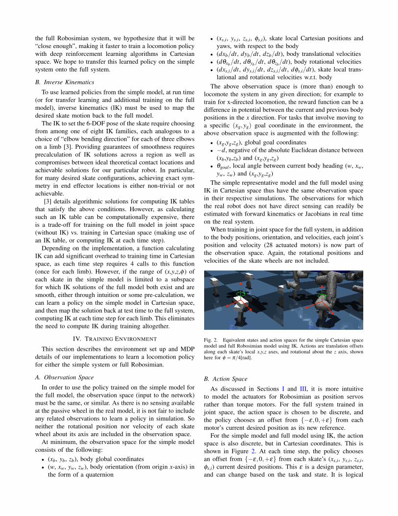
Fig. 2. Equivalent states and action spaces for the simple Cartesian spacemodel and full Robosimian model using IK. Actions are translation offsetsalong each skate’s local x,y,z axes, and rotational about the z axis, shownhere for φ = π/4[rad].

B. Action Space

As discussed in Sections I and III, it is more intuitiveto model the actuators for Robosimian as position servosrather than torque motors. For the full system trained injoint space, the action space is chosen to be discrete, andthe policy chooses an offset from {−ε,0,+ε} from eachmotor’s current desired position as its new reference.

For the simple model and full model using IK, the actionspace is also discrete, but in Cartesian coordinates. This isshown in Figure 2. At each time step, the policy choosesan offset from {−ε,0,+ε} from each skate’s (xs,i, ys,i, zs,i,φs,i) current desired positions. This ε is a design parameter,and can change based on the task and state. It is logical

for ys,i and φs,i to change by different offsets εy and εφ , forexample, due to the difference in units (meters vs. radians).A caveat is that the IK joint position differences of the fullmodel between time steps must be bounded. We note that asmall difference in the end effector location can have a largedifference in the IK solution, even when using the same IKfamily, if near a singularity. We seek to minimize these eventsby keeping the simple model’s workspace within smooth IKsolution spaces for the full model.

C. Reward Functions

We consider potential-based shaping functions of the form:

F(s,a,s′) = γΦ(s′)−Φ(s) (3)

to guarantee consistency with the optimal policy, as provedby Ng et. al in [16]. The real valued function Φ : S→R variesbetween tasks, with two such example tasks consisting of:

1) maximizing forward velocity in the x direction:

Φ(s) =xb

∆t(4)

2) minimizing the distance to a target goal (xg,yg,zg):

Φ(s) =−√(xb− xg)2 +(yb− yg)2 +(zb− zg)2 (5)

This reward scheme gives dense rewards at each timestep, towards ensuring the optimal policy is learned, andallows us to avoid complicated hand-crafted reward functionswith many variables that ultimately output a single numberanyway. Such schemes can result in slow training and sub-optimal behavior.

D. Implementation Details

We use a combination of OpenAI Gym [17] to representthe MDP and MuJoCo [7] as the physics engine for trainingand simulation purposes. We additionally use the OpenAIBaselines [18] implementation of PPO (PPO2) as a basis,making some key modifications for our system. Our neuralnetwork architecture is the default Multi-Layer Perceptron(MLP), which consists of 2 fully connected hidden layers of64 neurons each, with tanh activation. The policy and valuenetworks both have this same network structure.

The default design parameters of these implementationsare kept the same, while perhaps not producing the mostoptimal or time-efficient policies for our system, to showthat intuitively reducing the action space has a large effecton training time and policy robustness.

V. RESULTS

We seek to compare the training times and robustness oflearned policies for the following systems:• SS: Simple “representative” system• FS in JS: Full system trained in joint space• FS in CS: Full system trained in Cartesian space with

IK (to set joints)We also seek to evaluate how well the learned policy of

the simple system transfers to the full system with inverse

kinematics. SS and FS in CS always have the same obser-vation and action spaces, for fair comparisons. We considertasks of skating at maximum velocity in the +x direction,and of locomoting to a particular goal location (xg,yg). Allpolicies along with additional comparisons to other controlmethods are shown in the supplementary video for this paper.

A. Skate Straight

First we consider the task of maximizing forward velocityin the +x direction. The observation and action spaces areas detailed in Sections IV-A and IV-B, with ε = 0.01. Theaction space for SS and FS in CS is limited to a ±0.1[m]offset of ys,i and ±0.3[rad] offset of φs,i for each skate fromit’s given starting position, with xs,i and zs,i fixed, to matchthe constraints used in designing skating motions for forwardlocomotion in [6]. The action space for FS in JS is boundedonly by the joint limits. Training on FS in JS also enforcesearly termination of an episode if any self-collisions aredetected, or if contact occurs with the ground from any partof the robot other than the skates. The reward at each timestep is a potential-based shaping function where Φ is as inEquation 4, resulting in:

F(s,a,s′) =x′b− xb

∆t, (6)

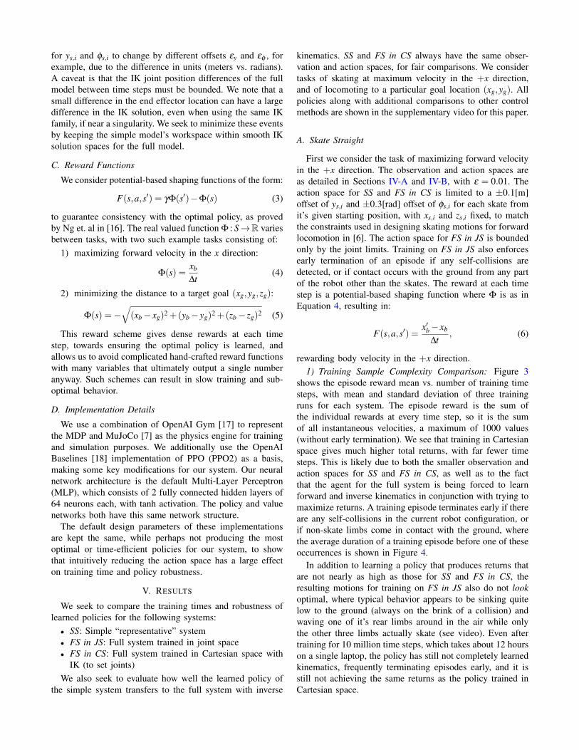
rewarding body velocity in the +x direction.1) Training Sample Complexity Comparison: Figure 3

shows the episode reward mean vs. number of training timesteps, with mean and standard deviation of three trainingruns for each system. The episode reward is the sum ofthe individual rewards at every time step, so it is the sumof all instantaneous velocities, a maximum of 1000 values(without early termination). We see that training in Cartesianspace gives much higher total returns, with far fewer timesteps. This is likely due to both the smaller observation andaction spaces for SS and FS in CS, as well as to the factthat the agent for the full system is being forced to learnforward and inverse kinematics in conjunction with trying tomaximize returns. A training episode terminates early if thereare any self-collisions in the current robot configuration, orif non-skate limbs come in contact with the ground, wherethe average duration of a training episode before one of theseoccurrences is shown in Figure 4.

In addition to learning a policy that produces returns thatare not nearly as high as those for SS and FS in CS, theresulting motions for training on FS in JS also do not lookoptimal, where typical behavior appears to be sinking quitelow to the ground (always on the brink of a collision) andwaving one of it’s rear limbs around in the air while onlythe other three limbs actually skate (see video). Even aftertraining for 10 million time steps, which takes about 12 hourson a single laptop, the policy has still not completely learnedkinematics, frequently terminating episodes early, and it isstill not achieving the same returns as the policy trained inCartesian space.

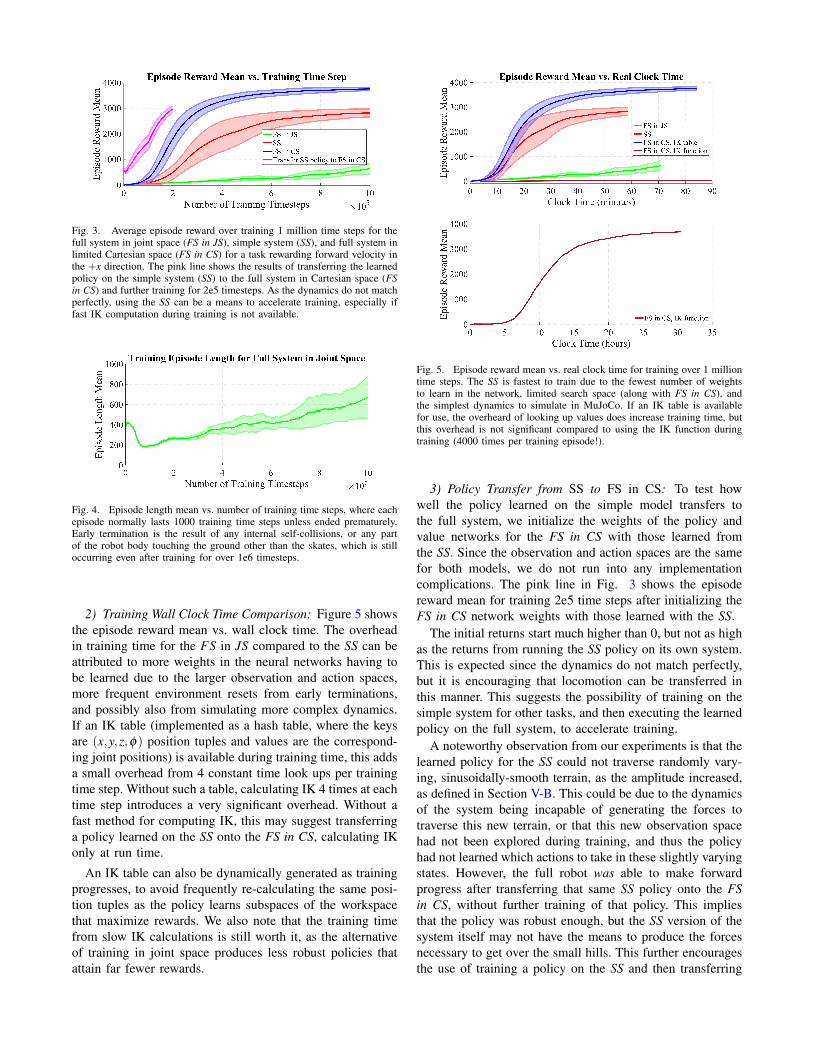
Fig. 3. Average episode reward over training 1 million time steps for thefull system in joint space (FS in JS), simple system (SS), and full system inlimited Cartesian space (FS in CS) for a task rewarding forward velocity inthe +x direction. The pink line shows the results of transferring the learnedpolicy on the simple system (SS) to the full system in Cartesian space (FSin CS) and further training for 2e5 timesteps. As the dynamics do not matchperfectly, using the SS can be a means to accelerate training, especially iffast IK computation during training is not available.

Fig. 4. Episode length mean vs. number of training time steps, where eachepisode normally lasts 1000 training time steps unless ended prematurely.Early termination is the result of any internal self-collisions, or any partof the robot body touching the ground other than the skates, which is stilloccurring even after training for over 1e6 timesteps.

2) Training Wall Clock Time Comparison: Figure 5 showsthe episode reward mean vs. wall clock time. The overheadin training time for the FS in JS compared to the SS can beattributed to more weights in the neural networks having tobe learned due to the larger observation and action spaces,more frequent environment resets from early terminations,and possibly also from simulating more complex dynamics.If an IK table (implemented as a hash table, where the keysare (x,y,z,φ) position tuples and values are the correspond-ing joint positions) is available during training time, this addsa small overhead from 4 constant time look ups per trainingtime step. Without such a table, calculating IK 4 times at eachtime step introduces a very significant overhead. Without afast method for computing IK, this may suggest transferringa policy learned on the SS onto the FS in CS, calculating IKonly at run time.

An IK table can also be dynamically generated as trainingprogresses, to avoid frequently re-calculating the same posi-tion tuples as the policy learns subspaces of the workspacethat maximize rewards. We also note that the training timefrom slow IK calculations is still worth it, as the alternativeof training in joint space produces less robust policies thatattain far fewer rewards.

Fig. 5. Episode reward mean vs. real clock time for training over 1 milliontime steps. The SS is fastest to train due to the fewest number of weightsto learn in the network, limited search space (along with FS in CS), andthe simplest dynamics to simulate in MuJoCo. If an IK table is availablefor use, the overheard of looking up values does increase training time, butthis overhead is not significant compared to using the IK function duringtraining (4000 times per training episode!).

3) Policy Transfer from SS to FS in CS: To test howwell the policy learned on the simple model transfers tothe full system, we initialize the weights of the policy andvalue networks for the FS in CS with those learned fromthe SS. Since the observation and action spaces are the samefor both models, we do not run into any implementationcomplications. The pink line in Fig. 3 shows the episodereward mean for training 2e5 time steps after initializing theFS in CS network weights with those learned with the SS.

The initial returns start much higher than 0, but not as highas the returns from running the SS policy on its own system.This is expected since the dynamics do not match perfectly,but it is encouraging that locomotion can be transferred inthis manner. This suggests the possibility of training on thesimple system for other tasks, and then executing the learnedpolicy on the full system, to accelerate training.

A noteworthy observation from our experiments is that thelearned policy for the SS could not traverse randomly vary-ing, sinusoidally-smooth terrain, as the amplitude increased,as defined in Section V-B. This could be due to the dynamicsof the system being incapable of generating the forces totraverse this new terrain, or that this new observation spacehad not been explored during training, and thus the policyhad not learned which actions to take in these slightly varyingstates. However, the full robot was able to make forwardprogress after transferring that same SS policy onto the FSin CS, without further training of that policy. This impliesthat the policy was robust enough, but the SS version of thesystem itself may not have the means to produce the forcesnecessary to get over the small hills. This further encouragesthe use of training a policy on the SS and then transferring

it to the full system for other tasks.

B. Skate To Goal Under Uncertainty

The next task we consider is locomoting the system fromthe origin (0,0) to a goal location (xg,yg), in particular(5,0)[m], over randomly varying, sinusoidally-smooth ter-rain with varying friction coefficients. For this task, theobservation spaces from the maximum velocity skating taskare augmented with the global goal coordinates, negativedistance to the goal from the robot’s current location, and theangle between the robot’s heading and the goal, as discussedin the latter part of Section IV-A. The action spaces areleft unchanged, as the limited spaces for SS and FS in CSshould be enough to locomote the system to the goal (it isalways possible to increase ranges, or allow x and z skateposition changes if the terrain is too rough). The reward ateach time step is again a potential-based function, with Φ asin Equation 5, where we assume zg = zb, resulting in:

F(s,a,s′) =−√(x′b− xg)2 +(y′b− yg)2

−(−√

(xb− xg)2 +(yb− yg)2)(7)

rewarding a decrease in the distance to the goal, and penal-izing moving away from the goal.

We train the policy to reach the goal (5,0) for 2 milliontime steps over smooth, sinusoidal terrain with amplitudeA = 0.1 [m], period 2π [m] in both x and y directions, andcoefficient of friction µ ∈ [0.5,1]. The terrain is randomlygenerated and moved in the xy plane by (δx,δy) ∈ [−1,1][m] at the start of each training episode (environment reset),on top of random perturbations of the joints, positions, andvelocities of the initial states. An episode is consideredcompleted when (xb,yb) is within 0.2 meters of (xg,yg), orwhen the episode times out after 1000 time steps.

We then test the policy over the same family of smoothsinusoidally varying terrain now also varying amplitude A ∈[0,0.2] [m] (the period 2π [m] and coefficient of frictionrange µ ∈ [0.5,1] are unchanged), and compare results withruns of our previously designed open-loop trajectory tolocomote the system 5 meters forwards from [6].

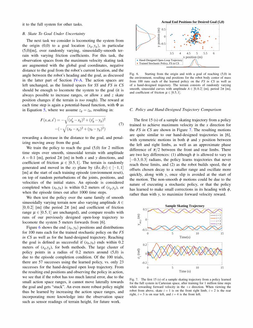
Figure 6 shows the end (xb,yb) positions and distributionsfor 100 runs each for the trained stochastic policy on the FSin CS as well as for the hand-designed trajectory. Reachingthe goal is defined as successful if (xb,yb) ends within 0.2meters of (xg,yg), for both methods. The large cluster ofpolicy points in a radius of 0.2 meters around (5,0) isdue to the episode completion condition. Of the 100 trials,there are 57 successes using the learned policy, vs. only 23successes for the hand-designed open loop trajectory. Fromthe resulting end positions and observing the policy in action,we see that if the robot has too much lateral error, due to thesmall action space ranges, it cannot move laterally towardsthe goal and gets “stuck”. An even more robust policy mightthus be learned by increasing the action space ranges, andincorporating more knowledge into the observation spacesuch as sensor readings of terrain height, for future work.

3.5 4 4.5 5 5.5 6x position (m)

-0.5

0

0.5

y po

sitio

n (m

)

Actual End Positions for Desired Goal (5,0)

Hand-Designed Open-Loop TrajectoryTrained Stochastic Policy, FS in CS

Fig. 6. Starting from the origin and with a goal of reaching (5,0) inthe environment, resulting end positions for the robot body center of massfrom 100 runs each of the learned policy on the FS in CS as well asof a hand-designed trajectory. The terrain consists of randomly varyingsmooth, sinusoidal curves with amplitude A ∈ [0,0.2] [m], period 2π [m],and coefficient of friction µ ∈ [0.5,1].

C. Policy and Hand-Designed Trajectory Comparison

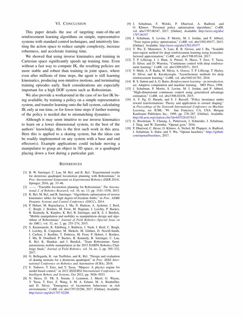
The first 15 (s) of a sample skating trajectory from a policytrained to achieve maximum velocity in the x direction forthe FS in CS are shown in Figure 7. The resulting motionsare quite similar to our hand-designed trajectories in [6],with symmetric motions in both φ and y position betweenthe left and right limbs, as well as an approximate phasedifference of π/2 between the front and rear limbs. Thereare two key differences: (1) although φ is allowed to vary in[−0.3,0.3] radians, the policy learns trajectories that neverreach those limits, and (2) as the robot builds speed, the φ

offsets chosen decay to a smaller range and oscillate morequickly, along with y, once slip is avoided at the start ofthe motion. The non-smooth φ motions could be due to thenature of executing a stochastic policy, or that the policyhas learned to make small corrections in its heading with φ ,rather than with y, to maximize forward velocity reward.

0 5 10 15Time(s)

-0.5

0

0.5

y ee,i (

m)

Sample Skating Trajectory

0 5 10 15Time (s)

-0.2

0

0.2

i (ra

d)

i = 1i = 2i = 3i = 4

Fig. 7. The first 15 (s) of a sample skating trajectory from a policy learnedfor the full system in Cartesian space, after training for 1 million time stepswhile rewarding forward velocity in the +x direction. When viewing therobot from above, skate i = 1 is on the front right limb, i = 2 is the rearright, i = 3 is on rear left, and i = 4 is the front left.

VI. CONCLUSION

This paper details the use of targeting state-of-the-artreinforcement learning algorithms on simple, representativesystems with standard control techniques, and intuitively lim-iting the action space to reduce sample complexity, increaserobustness, and accelerate training time.

We showed that using inverse kinematics and training inCartesian space significantly speeds up training time. Evenwithout a fast way to compute IK, the resulting policies aremore stable and robust than training in joint space, whereeven after millions of time steps, the agent is still learningkinematics, producing non-intuitive motions, and terminatingtraining episodes early. Such considerations are especiallyimportant for a high DOF system such as Robosimian.

We also provide a workaround in the case of no fast IK be-ing available, by training a policy on a simple representativesystem, and transfer learning onto the full system, calculatingIK only at run time, or for fewer time steps if further trainingof the policy is needed due to mismatching dynamics.

Although it may seem intuitive to use inverse kinematicsto learn on a lower dimensional system, to the best of theauthors’ knowledge, this is the first such work in this area.Here this is applied to a skating system, but the ideas canbe readily implemented on any system with a base and endeffector(s). Example applications could include moving amanipulator to grasp an object in 3D space, or a quadrupedplacing down a foot during a particular gait.

REFERENCES

[1] B. W. Satzinger, C. Lau, M. Byl, and K. Byl, “Experimental resultsfor dexterous quadruped locomotion planning with Robosimian,” inProc. Inernational Symposium on Experimental Robotics (ISER 2014).Springer, 2016, pp. 33–46.

[2] ——, “Tractable locomotion planning for Robosimian,” The Interna-tional J. of Robotics Research, vol. 34, no. 13, pp. 1541–1558, 2015.

[3] K. Byl, M. Byl, and B. Satzinger, “Algorithmic optimization of inversekinematics tables for high degree-of-freedom limbs,” in Proc. ASMEDynamic Systems and Control Conference (DSCC), 2014.

[4] P. Hebert, M. Bajracharya, J. Ma, N. Hudson, A. Aydemir, J. Reid,C. Bergh, J. Borders, M. Frost, M. Hagman, J. Leichty, P. Backes,B. Kennedy, K. Karplus, K. Byl, B. Satzinger, and K. S. J. Burdick,“Mobile manipulation and mobility as manipulation–design and algo-rithms of Robosimian,” Journal of Field Robotics (Special Issue onthe DRC), vol. 32, no. 2, pp. 255–274, 2015.

[5] S. Karumanchi, K. Edelberg, I. Baldwin, J. Nash, J. Reid, C. Bergh,J. Leichty, K. Carpenter, M. Shekels, M. Gildner, D. Newill-Smith,J. Carlton, J. Koehler, T. Dobreva, M. Frost, P. Hebert, J. Borders,J. Ma, B. Douillard, P. Backes, B. Kennedy, B. Satzinger, C. Lau,K. Byl, K. Shankar, and J. Burdick, “Team Robosimian: Semi-autonomous mobile manipulation at the 2015 DARPA Robotics Chal-lenge finals,” Journal of Field Robotics, vol. 34, no. 2, pp. 305–332,2017.

[6] G. Bellegarda, K. van Teeffelen, and K. Byl, “Design and evaluationof skating motions for a dexterous quadruped,” in Proc. IEEE Inter-national Conference on Robotics and Automation (ICRA), 2018.

[7] E. Todorov, T. Erez, and Y. Tassa, “Mujoco: A physics engine formodel-based control,” in 2012 IEEE/RSJ International Conference onIntelligent Robots and Systems, Oct 2012, pp. 5026–5033.

[8] N. Heess, D. TB, S. Sriram, J. Lemmon, J. Merel, G. Wayne,Y. Tassa, T. Erez, Z. Wang, S. M. A. Eslami, M. A. Riedmiller,and D. Silver, “Emergence of locomotion behaviours in richenvironments,” CoRR, vol. abs/1707.02286, 2017. [Online]. Available:http://arxiv.org/abs/1707.02286

[9] J. Schulman, F. Wolski, P. Dhariwal, A. Radford, andO. Klimov, “Proximal policy optimization algorithms,” CoRR,vol. abs/1707.06347, 2017. [Online]. Available: http://arxiv.org/abs/1707.06347

[10] J. Schulman, S. Levine, P. Moritz, M. I. Jordan, and P. Abbeel,“Trust region policy optimization,” CoRR, vol. abs/1502.05477, 2015.[Online]. Available: http://arxiv.org/abs/1502.05477

[11] Y. Wu, E. Mansimov, S. Liao, R. B. Grosse, and J. Ba, “Scalabletrust-region method for deep reinforcement learning using kronecker-factored approximation,” CoRR, vol. abs/1708.05144, 2017.

[12] T. P. Lillicrap, J. J. Hunt, A. Pritzel, N. Heess, T. Erez, Y. Tassa,D. Silver, and D. Wierstra, “Continuous control with deep reinforce-ment learning,” CoRR, vol. abs/1509.02971, 2015.

[13] V. Mnih, A. P. Badia, M. Mirza, A. Graves, T. P. Lillicrap, T. Harley,D. Silver, and K. Kavukcuoglu, “Asynchronous methods for deepreinforcement learning,” CoRR, vol. abs/1602.01783, 2016.

[14] R. S. Sutton and A. G. Barto, Reinforcement learning - an introduction,ser. Adaptive computation and machine learning. MIT Press, 1998.

[15] J. Schulman, P. Moritz, S. Levine, M. I. Jordan, and P. Abbeel,“High-dimensional continuous control using generalized advantageestimation,” CoRR, vol. abs/1506.02438, 2015.

[16] A. Y. Ng, D. Harada, and S. J. Russell, “Policy invariance underreward transformations: Theory and application to reward shaping,”in Proceedings of the Sixteenth International Conference on MachineLearning, ser. ICML ’99. San Francisco, CA, USA: MorganKaufmann Publishers Inc., 1999, pp. 278–287. [Online]. Available:http://dl.acm.org/citation.cfm?id=645528.657613

[17] G. Brockman, V. Cheung, L. Pettersson, J. Schneider, J. Schulman,J. Tang, and W. Zaremba, “Openai gym,” 2016.

[18] P. Dhariwal, C. Hesse, O. Klimov, A. Nichol, M. Plappert, A. Radford,J. Schulman, S. Sidor, and Y. Wu, “Openai baselines,” https://github.com/openai/baselines, 2017.