GUIDE TO PROJECT EVALUATION - · PDF file09.12.1994 · Part 5 provides a guide to the conditions under which the use of macroeconom- ic models in project evaluation is appropriate

GUIDE TO PROJECT EVALUATION

Part 5: Impact on National and Regional Economies

Guide to Project Evaluation Part 5: Impact on National and

Regional Economies

Guide to Project Evaluation Part 5: Impact on National and Regional Economies Summary Part 5 provides a guide to the conditions under which the use of macro-economic models in project evaluation is appropriate and how they can be applied. Major transport infrastructure projects often significantly alter the economies of regions in which they are located and, if large enough, the national economy as well. These effects may not be fully captured by standard benefit-cost analysis evaluations. One method of estimating economic impacts of large transport infrastructure projects is the use of economy-wide type models. A class of model known as ‘computable general equilibrium’ has been used to analyse economy wide impacts. Keywords transport project evaluation, benefit cost analysis, impact analysis, economy-wide models, input-output (I-O) analysis, computable general equilibrium models First Published 2005 © Austroads Inc. 2005 This work is copyright. Apart from any use as permitted under the Copyright Act 1968, no part may be reproduced by any process without the prior written permission of Austroads. National Library of Australia Cataloguing-in-Publication data: ISBN 0 85588 740 0 Austroads Project No. TP1050 Austroads Publication No. AGPE05/05 Authors Dimitris Tsolakis Katrina Preski Published by Austroads Incorporated Level 9, Robell House 287 Elizabeth Street Sydney NSW 2000 Australia Phone: +61 2 9264 7088 Fax: +61 2 9264 1657 Email: [email protected] www.austroads.com.au This Guide is produced by Austroads as a general guide. Its application is discretionary. Road authorities may vary their practice according to local circumstances and policies. Austroads believes this publication to be correct at the time of printing and does not accept responsibility for any consequences arising from the use of information herein. Readers should rely on their own skill and judgement to apply information to particular issues.

mailto:[email protected]

CONTENTS 1. INTRODUCTION ................................................................................................................................... 1

2. PARTIAL – VERSUS GENERAL-EQUILIBRIUM ANALYSIS ...................................................... 2

3. REASONS TO UNDERTAKE BCA AND MACROECONOMIC MODELLING .......................... 3

4. COSTS OF UNDERTAKING CGE MODELLING............................................................................ 4

5. POSITIONING MACROECONOMIC MODELLING IN THE PROJECT EVALUATION PROCESS .............................................................................................................................................. 5

6. STATE/TERRITORY AND REGIONAL DETAIL OF CGE MODELS .......................................... 7

7. CGE MODELS USED IN THE TRANSPORT SECTOR ................................................................ 8

8. RECENT EXAMPLES .......................................................................................................................... 9

COMMENTARIES ........................................................................................................................................ 10

COMMENTARY A: WHAT IS GE ANALYSIS MODELLING? ............................................................. 10

A.1 Economic principles ............................................................................................................. 10 A.2 Exogenous variables ............................................................................................................ 10 A.3 Dynamics ............................................................................................................................. 11 A.4 Structure of GE models ........................................................................................................ 11 A.5 Input-Output (I-O) analysis ................................................................................................... 12 A.6 Transport sector detail .......................................................................................................... 13 A.7 Treatment of externalities in GE models ............................................................................... 13 A.8 Results obtained from CGE models ..................................................................................... 14 A.9 What CGE models can not do .............................................................................................. 14 A.10 Model complexity ................................................................................................................. 15 A.11 Updating models .................................................................................................................. 16 A.12 Double-counting issue .......................................................................................................... 16

COMMENTARY B: REASONS TO UNDERTAKE BCA AND MACROECONOMIC MODELLING17

B.1 Fiscal Impact of Transport Projects ...................................................................................... 17 B.2 Checklist of When to Undertake CGE Modelling .................................................................. 18

COMMENTARY C: POSITIONING MACROECONOMIC MODELLING IN THE PROJECT EVALUATION PROCESS ....................................................................................... 19

COMMENTARY D: STATE/TERRITORY AND REGIONAL DETAIL OF CGE MODELS .............. 22

D.1 Treatment of State/Territory and Regional Interactions in CGE Models ................................ 22

COMMENTARY E: CGE MODELS USED IN THE TRANSPORT SECTOR ..................................... 25

E.1 Centre of Policy Studies (CoPS)........................................................................................... 25 E.2 Sources of Information for CGE models used by CoPS ........................................................ 27 E.3 Econtech’s Murphy MM600+ Model ..................................................................................... 27 E.4 National Economics Multi-purpose Model (IMP) ................................................................... 28 E.5 Inventory of CGE models used to analyse transport issues .................................................. 29

COMMENTARY F: RECENT EXAMPLES ............................................................................................... 31

F.1 Melbourne City Link project .................................................................................................. 31 F.2 Economic impacts of improved port efficiency ...................................................................... 32 F.3 The role of transport infrastructure in Australia’s economic growth ....................................... 33

Guide to Project Evaluation: Part 5 - Impact on the National and Regional Economies

A u s t r o a d s 2 0 0 5

— 1 —

1. INTRODUCTION Major transport infrastructure projects often significantly alter the economies of the regions in which they are located, and if large enough, the national economy as well. When evaluating transport infrastructure projects which are predicted to impact the economy on a macroeconomic scale, decision-makers may require a wider test of ‘public benefit’ of the project, such as employment, regional development, and the effects on other industries in the region.

National (or state/regional) economy-wide models such as Computable General Equilibrium (CGE) models can be used to analyse the far-reaching impacts of such projects for the rest of the economy (eg impacts for private consumption, investment, exports, imports, inflation, total GDP and GDP by industry). This information is normally not available from standard BCA evaluations.

Unlike other Parts of the Guide to Project Evaluation, Part 5 is not intended to enable project evaluators to build or operate economy-wide CGE models. Rather, its intention is to inform them of available models, allow them to identify when use of such models is warranted, and to enable them to engage in informed discussion with the purveyors of such models.

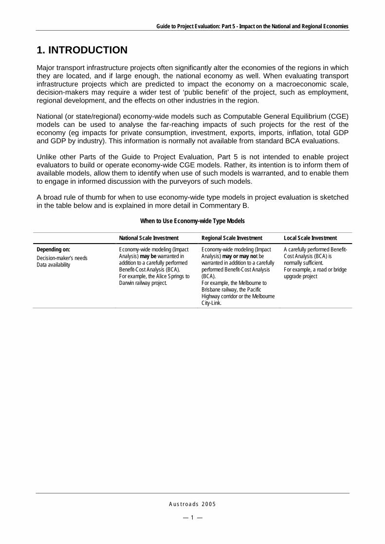
A broad rule of thumb for when to use economy-wide type models in project evaluation is sketched in the table below and is explained in more detail in Commentary B.

When to Use Economy-wide Type Models

National Scale Investment Regional Scale Investment Local Scale Investment

Depending on: Decision-maker’s needs Data availability

Economy-wide modeling (Impact Analysis) may be warranted in addition to a carefully performed Benefit-Cost Analysis (BCA). For example, the Alice Springs to Darwin railway project.

Economy-wide modeling (Impact Analysis) may or may not be warranted in addition to a carefully performed Benefit-Cost Analysis (BCA). For example, the Melbourne to Brisbane railway, the Pacific Highway corridor or the Melbourne City-Link.

A carefully performed Benefit-Cost Analysis (BCA) is normally sufficient. For example, a road or bridge upgrade project


A u s t r o a d s 2 0 0 5

— 2 —

2. PARTIAL – VERSUS GENERAL-EQUILIBRIUM ANALYSIS Partial equilibrium (PE) analysis is the methodological approach that broadly underlies traditional benefit-cost analysis (BCA) applications. In PE analysis, benefits are estimated by examining only the ‘first-round’ or ‘initial’ impacts of project expenditure. Subsequent rounds of expenditure are ignored on the grounds that (normally) all benefits from this source are balanced by costs. PE analysis concentrates on the effect of changes in individual markets or industries, holding all other things equal.

BCA is normally performed to yield the following three summary output evaluation measures:

Net Present Value (NPV) of project benefits and costs

Benefit-Cost Ratio (BCR)

Internal Rate of Return (IRR) of project investment.

General equilibrium (GE) analysis, and CGE models developed to enable GE analysis, are economy wide (eg. national, state or regional) mathematical models, which are employed to perform simulations related to the behaviour of industries (producers), consumers and governments in response to economic changes or policy and other ‘shocks’. These shocks may include a large transport infrastructure investment that has the capacity to affect other sectors of the economy, eg agriculture, manufacturing, mining, tourism and construction industries both within and across jurisdictions.

A description of the economic principles, structure and complexity of CGE models is provided in Commentary A.

[see Commentary A]


A u s t r o a d s 2 0 0 5

— 3 —

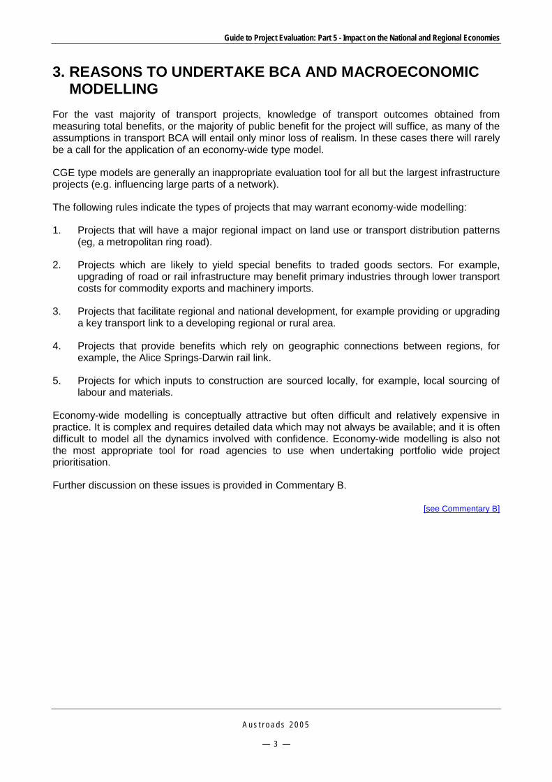
3. REASONS TO UNDERTAKE BCA AND MACROECONOMIC MODELLING

For the vast majority of transport projects, knowledge of transport outcomes obtained from measuring total benefits, or the majority of public benefit for the project will suffice, as many of the assumptions in transport BCA will entail only minor loss of realism. In these cases there will rarely be a call for the application of an economy-wide type model.

CGE type models are generally an inappropriate evaluation tool for all but the largest infrastructure projects (e.g. influencing large parts of a network).

The following rules indicate the types of projects that may warrant economy-wide modelling:

1. Projects that will have a major regional impact on land use or transport distribution patterns (eg, a metropolitan ring road).

2. Projects which are likely to yield special benefits to traded goods sectors. For example, upgrading of road or rail infrastructure may benefit primary industries through lower transport costs for commodity exports and machinery imports.

3. Projects that facilitate regional and national development, for example providing or upgrading a key transport link to a developing regional or rural area.

4. Projects that provide benefits which rely on geographic connections between regions, for example, the Alice Springs-Darwin rail link.

5. Projects for which inputs to construction are sourced locally, for example, local sourcing of labour and materials.

Economy-wide modelling is conceptually attractive but often difficult and relatively expensive in practice. It is complex and requires detailed data which may not always be available; and it is often difficult to model all the dynamics involved with confidence. Economy-wide modelling is also not the most appropriate tool for road agencies to use when undertaking portfolio wide project prioritisation.

Further discussion on these issues is provided in Commentary B.

[see Commentary B]


A u s t r o a d s 2 0 0 5

— 4 —

4. COSTS OF UNDERTAKING CGE MODELLING Cost of CGE modelling applications depends on the specifics of the project, which may take from one day to many months to complete. The most important factor is the nature of the required modifications to the commercially available models. For most projects, with a transport or non-transport flavour, some modifications to the regional or sectoral model detail are necessary. Experienced modellers can usually implement such changes quickly. The cost of a relatively straightforward CGE analysis for a specific project is estimated to be between $10,000 and $50,000 (in 2004 dollars) depending on model refinements, complexity of the project (i.e. spatial scale) and number of scenario cases to be modelled.

For use within an organisation, the basic Centre of Policy Studies (CoPS) model, for example, can be used off the shelf at a reasonable cost. However, training staff to operate the model could be time-consuming and costly. Depending on the level of detail, data collection and analysis could also be time-consuming and costly.

BTE (1999) concludes that the application of economy-wide models are often costly, in particular, in relation to the cost attached to the effort that people make to understand the model as well as its application.


A u s t r o a d s 2 0 0 5

— 5 —

5. POSITIONING MACROECONOMIC MODELLING IN THE PROJECT EVALUATION PROCESS

Economy-wide modelling of large-scale road investments can be useful to supplement or complement standard BCA assessments. As such they can be undertaken once a BCA has been completed.

For a large project identified by a BCA to be economically viable, CGE analysis can serve as an extension to the BCA assessment and can provide a policy impact analysis of the particular investment.

The transport sector is an obvious candidate for GE modelling because of its implications for other sectors of the economy, including agriculture, manufacturing and mining. Some of the most important industries to consider are described below.

Industry Impacts of Transport Projects

Industries Effects

Construction Increased activity – increased employment and production eg steel Freeing up of resources post construction

Agriculture Increased transport options Lower transport costs Reclamation of land for road/rail projects Road or rail reserve can cause division or severance of properties

Mining Increased transport options Lower transport costs

Manufacturing Increased transport options Lower transport costs

Tourism Increased mobility/travel options Aesthetics – i.e. decline of natural environment

Improved transport services induce greater efficiency in input use by transport-using firms, and from gains in accessibility, market expansion, and restructuring of activities as the transport improvements flow through the broader economy (see figure on page 6).

The key feature of the figure on page 6 is gains from trade resulting from infrastructure improvements. Specialisation and trade are economically feasible only to the extent that efficiency benefits exceed the cost of interregional shipment, and the speed and reliability of shipment make it possible to coordinate production schedules across long distances. Thus, freight cost reductions and quality improvements lead to efficiency gains from trade (Lakshmanan and Anderson, 2002). These gains then lead to effects such as export and import expansion, investment in innovation and technical diffusion and economies of scale. See Commentary C.

[see Commentary C]


A u s t r o a d s 2 0 0 5

— 6 —

Indirect Impacts of Infrastructure on Macroeconomic Growth

Transport Infrastructure Investments

Improved Freight/Service Attributes(lower costs, time savings, more

reliability, new services)

Increased Accessibility and Market Expansion(Gains from Trade)

Improved Labour Supply

Export & Import Expansion &

Competitive Pressures

Expanded Production

Economic Restructuring(Entry/exit of

firms)

Total Factor Productivity & GDP Growth

Increasing Returns to

Scale & Spatial

Agglomeration Effects

Innovation &

Technical Diffusion

Source: Lakshmanan and Anderson, 2002


A u s t r o a d s 2 0 0 5

— 7 —

6. STATE/TERRITORY AND REGIONAL DETAIL OF CGE MODELS

CGE analysis models use a set of input-output (I-O) tables (of national accounts) as their primary data source. These I-O tables are produced at the national level by the Australian Bureau of Statistics.

CGE models can be produced for the State/Territory level. However, the limiting factor is the availability of the I-O data at the State and regional level depending on user preference/needs.

More detail about how well CGE model developments can handle the need for applying these models at the state and regional levels are presented in Commentary D.

[see Commentary D]


A u s t r o a d s 2 0 0 5

— 8 —

7. CGE MODELS USED IN THE TRANSPORT SECTOR There are two basic classes of economy-wide models used to represent and describe the macroeconomic effects at a national or regional level. These can be broadly described as econometric models and Input-Output (I-O) based models. The former mostly comprise sets of mathematical/statistical relationships that are estimated to obtain key summary parameters (e.g. elasticities) describing the underlying economic structure of markets/sectors1. The latter class mostly comprises simulation type models used to simulate the impacts of policies and shifts in the flows of inputs and outputs (goods and services) at an economy-wide level2. Choice of model depends on the nature of the policy question asked. Generally speaking, econometric models are useful for generating key parameters and forecasts as inputs to I-O type models which are used to perform economy-wide (national or regional) impact analysis.

The inter-sectoral nature of transport interactions in the economy requires a modelling framework that takes into account all flows within the economy when transport policy impact analysis is undertaken. Input-Output (I-O) models based on the national accounts provide such a framework. While standard I-O analysis is still undertaken, the I-O platform has spawned many economy-wide model types. The distinction between commercially available economy-wide models relates to varying levels of development and complexity.

A class of economy-wide model known as Computable General Equilibrium (CGE) has been developed to analyse broader economic impacts. CGE models are usually developed for use by policy makers and planners in government agencies, treasuries and reserve/merchant banks. Essentially, these models help to predict the impacts of government policies or other ‘shocks’ related to transport investment on the whole economy.

CGE models are complex economy-wide models. It is not recommended that transport practitioners build or operate such models. If a transport project requires macroeconomic (CGE) type analysis, it is recommended that the practitioner enlist one of the specialist organisations that can undertake the CGE analysis. Some notable examples of economy-wide models that have been used in transport are:

Centre of Policy Studies (CoPS) at Monash University: CGE models include the MONASH, the MMRF-GREEN and the TERM models.

Econtech’s Murphy Model 600+ (MM600+).

National Economics IMP model. (This is not, strictly, a CGE model. The National Economics IMP model has been described as a type of integrated input-output and econometric modelling.)

While there are many other CGE models available for the Australian economy which the practitioner may procure, the purveyors of the models listed have expertise in policy impact analysis in the transport sector and have tailored their models for such applications.

[see Commentary E]

1 Econometric models are based on a series of equations that measure past relationships between variables such as consumer spending and gross national product, and then try to forecast how changes in one variable will affect the others. They are not generally used in policy impact analysis because most do not account for all flows within the economy.

2 I-O models are based on the national accounts so they are able to take into account all flows within the economy. The economy is a complex arrangement of inter-relationships between industries and agents. For all defined industries, the input-output transaction table at the core of the I-O model shows the inputs used by an industry to produce its output for a given time period.


A u s t r o a d s 2 0 0 5

— 9 —

8. RECENT EXAMPLES Three recent examples of CGE modelling are provided in Commentary F. These are as follows:

1. Melbourne City Link project (provided by the Centre of Policy Studies).

2. Economic impacts of improved port efficiency (provided by the Centre of Policy Studies).

3. The role of transport infrastructure in Australia’s economic growth (provided by National Economics).

[see Commentary F]


A u s t r o a d s 2 0 0 5

— 1 0 —

[back to Guidelines]

PART 5 COMMENTARIES

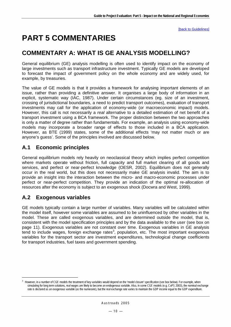
COMMENTARY A: WHAT IS GE ANALYSIS MODELLING? General equilibrium (GE) analysis modelling is often used to identify impact on the economy of large investments such as transport infrastructure investment. Typically GE models are developed to forecast the impact of government policy on the whole economy and are widely used, for example, by treasuries.

The value of GE models is that it provides a framework for analysing important elements of an issue, rather than providing a definitive answer. It organises a large body of information in an explicit, systematic way (IAC, 1987). Under certain circumstances (eg. size of an investment, crossing of jurisdictional boundaries, a need to predict transport outcomes), evaluation of transport investments may call for the application of economy-wide (or macroeconomic impact) models. However, this call is not necessarily a real alternative to a detailed estimation of net benefit of a transport investment using a BCA framework. The proper distinction between the two approaches is only a matter of degree rather than fundamentals. For example, an analysis using economy-wide models may incorporate a broader range of effects to those included in a BCA application. However, as BTE (1999) states, some of the additional effects ‘may not matter much or are anyone’s guess’. Some of the principles involved are discussed below.

A.1 Economic principles

General equilibrium models rely heavily on neoclassical theory which implies perfect competition where markets operate without friction, full capacity and full market clearing of all goods and services, and perfect or near-perfect knowledge (OESR, 2002). Equilibrium does not generally occur in the real world, but this does not necessarily make GE analysis invalid. The aim is to provide an insight into the interaction between the micro- and macro-economic processes under perfect or near-perfect competition. They provide an indication of the optimal re-allocation of resources after the economy is subject to an exogenous shock (Docwra and West, 1999).

A.2 Exogenous variables

GE models typically contain a large number of variables. Many variables will be calculated within the model itself, however some variables are assumed to be uninfluenced by other variables in the model. These are called exogenous variables, and are determined outside the model, that is, consistent with the model specification principles and by the data available to the user (see box on page 11). Exogenous variables are not constant over time. Exogenous variables in GE analysis tend to include wages, foreign exchange rates3, population, etc. The most important exogenous variables for the transport sector are investment expenditures, technological change coefficients for transport industries, fuel taxes and government spending.

3 However, in a number of CGE models the treatment of key variables would depend on the ‘model closure’ specification (see box below). For example, when

simulating for long term solutions, real wages are likely to become an endogenous variable. Also, in some CGE models (e.g. CoPS 2003), the nominal exchange rate is declared as an exogenous variable (as the numeraire), but the real exchange rate varies to maintain the GDP income equal to the GDP expenditure.


A u s t r o a d s 2 0 0 5

— 1 1 —

How GE Analysis Models Work

At the core of the GE analysis model is a set of equations describing the behaviour of various economic agents (for example industries, consumers and governments) when faced with changes in key economic variables, for example, and most importantly, relative prices. Typically, consumers maximise utility subject to a budget constraint, and industries maximise revenues (or minimise costs) subject to their production functions (technologies). The core behavioural equations are supplemented with market clearing equations that equate supply and demand in all commodity and factor markets. For example market clearing equations ensure that: demand for domestically-produced commodities equals their supply; demand for labour of each type across all industries is satisfied; and demand for capital in each industry is equal to supply (IAC, 1987).

The model is calibrated from a numerical database, the central core of which is a set of input-output (I-O) tables (of national accounts) showing, for a given year, the flows of primary (or intermediate) factors between groups and economic agents.

To obtain a solution to the model, the model’s equations are solved simultaneously. However, GE models have more variables than equations; this means that the user must specify the values of some variables. This set of user-specified exogenous variables is referred to as the model’s closure.

Closure plays an important role by creating the economic environment in which the policy scenario is set. In other words, the closure specifies some variables as exogenous to reflect various assumptions regarding the way economic agents behave, for example closure typically reflects assumptions about the government budget deficit, capital formation, wages and foreign currency prices.

Source: OESR, 2002.

A.3 Dynamics

A key means of discriminating between GE analysis models is their treatment of time within the economy. A comparative static model compares the economy at distinct points of time, without modelling any explicit time period or time path. Typically, the model compares the economy with a given policy change and without the policy change. The alternative category of models is that of the dynamic models. Dynamic models have inter-temporal links that show the adjustment path of a ‘shock’ over a specified timeframe.

Dynamic GE analysis models are run to show the response of the economy to an applied shock over various length of time. In GE modelling, a short run is normally taken to represent a modelling period of approximately two to three years, while a long run represents a period of eight to ten years (OESR, 2002). Most recently developed GE type models are dynamic. For example, the MMRF GREEN model is a dynamic model that can produce year-on-year dynamic simulations with a forecast period up to 2025. The National Economics IMP model is also fully dynamic producing results on an annual basis.

A.4 Structure of GE models

GE analysis models use a set of input-output (I-O) tables (of national accounts) as their primary data source. These tables show for a given year, the flows of primary (or intermediate) factors between groups and economic agents. I-O tables are essentially a disaggregation of the gross domestic product (GDP) account. Australian I-O tables are composed by the Australian Bureau of Statistics (ABS).


A u s t r o a d s 2 0 0 5

— 1 2 —

An I-O table includes four quadrants, which describe intermediate usage, final demand, primary inputs to production and primary inputs to final demand (see below). The primary inputs include wages and salaries, gross operating surplus and taxes. No industry operates in isolation; I-O table columns show an important link being the flow of industry output to other industries as inputs to further production (Sydney and Maina, 1994). These detailed inter-industry accounts are the strength of I-O data based analysis.

The key assumption of I-O tables is an open economy where supply meets demand. Since the value of the output of an industry must equal the sum of its inputs, row totals for an industry equal the corresponding column totals in the I-O tables (Sydney and Maina, 1994).

Simplified Input-output table

Intermediate Demand Final Demand

QUADRANT 1

INTERMEDIATEUSAGE

Agr

icul

ture

Wages, salaries and supplementsGross operating surplusCommodity taxes (net)Indirect taxes (net)Sales by final buyersComplementary imports and dutyAustralian ProductionCompeting imports and dutyTotal usage

AgricultureMiningManufacturingConstruction Services

Man

ufac

turin

g

Con

stru

ctio

n

Ser

vice

s

Min

ing

Cha

nge

in s

tock

s

Cap

ital e

xpen

ditu

re

Con

stru

ctio

n

Exp

orts

Inte

rmed

iate

usa

ge(s

ub-to

tal)

Tota

l sup

ply

Fina

l dem

and

(sub

-tota

l)

Inte

rmed

iate

in

puts

Prim

ary

inpu

ts QUADRANT 4

PRIMARY INPUTS TO FINAL DEMAND

QUADRANT 3

PRIMARY INPUTSTO PRODUCTION

QUADRANT 2

FINAL DEMAND

SUPPLY

USAGE

Source: BTCE, 1996b.

A.5 Input-Output (I-O) analysis

Simple input-output analysis can be considered a limited case of the more complicated GE analysis. In the I-O analysis, the I-O table is converted into a model of inter-industry response through the manipulation of the I-O database. I-O analysis involves the use of multipliers to calculate the overall economic impact of a project or policy change. Two common multipliers are used: multipliers that measure the industrial response to the change, and multipliers that measure in addition to the industrial response, the consumption-induced response (Woollett et al, 2002).

The advantage of I-O analysis is its ease of use and transparency. The weakness of I-O analysis is that it makes several assumptions – industries face a constant cost structure, the existence of unlimited quantities of labour and capital at fixed prices, and the amount of input which an industry uses is directly proportional to an industry’s output, under a fixed coefficient of technology (production function). I-O analysis omits other features of the economy such as the real exchange rate and its effect on imports and exports (BTCE 1996b).

Nevertheless I-O represents a simplified form of equilibrium, and it has been demonstrated that, particularly under ‘small region’ assumptions, the GE analysis solution converges to the I-O solution (Docwra and West 1999).


A u s t r o a d s 2 0 0 5

— 1 3 —

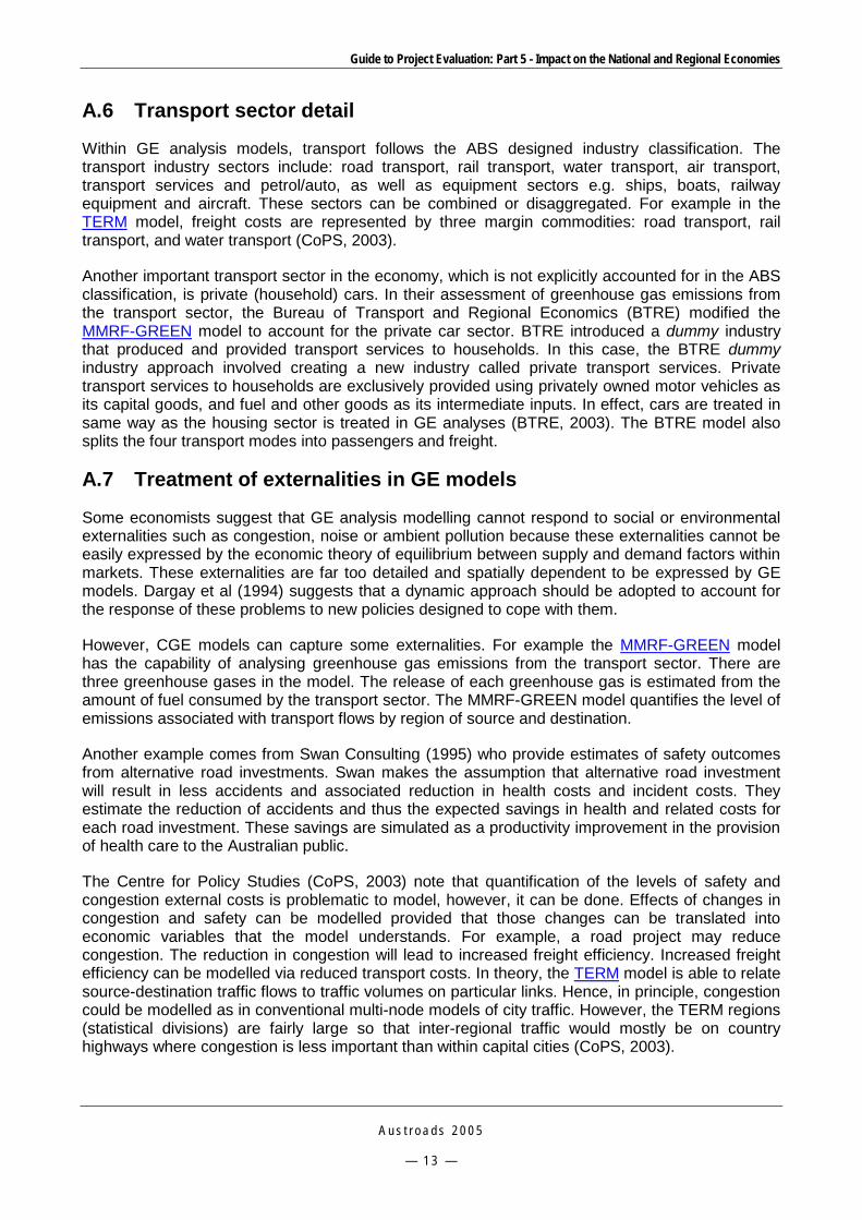
A.6 Transport sector detail

Within GE analysis models, transport follows the ABS designed industry classification. The transport industry sectors include: road transport, rail transport, water transport, air transport, transport services and petrol/auto, as well as equipment sectors e.g. ships, boats, railway equipment and aircraft. These sectors can be combined or disaggregated. For example in the TERM model, freight costs are represented by three margin commodities: road transport, rail transport, and water transport (CoPS, 2003).

Another important transport sector in the economy, which is not explicitly accounted for in the ABS classification, is private (household) cars. In their assessment of greenhouse gas emissions from the transport sector, the Bureau of Transport and Regional Economics (BTRE) modified the MMRF-GREEN model to account for the private car sector. BTRE introduced a dummy industry that produced and provided transport services to households. In this case, the BTRE dummy industry approach involved creating a new industry called private transport services. Private transport services to households are exclusively provided using privately owned motor vehicles as its capital goods, and fuel and other goods as its intermediate inputs. In effect, cars are treated in same way as the housing sector is treated in GE analyses (BTRE, 2003). The BTRE model also splits the four transport modes into passengers and freight.

A.7 Treatment of externalities in GE models

Some economists suggest that GE analysis modelling cannot respond to social or environmental externalities such as congestion, noise or ambient pollution because these externalities cannot be easily expressed by the economic theory of equilibrium between supply and demand factors within markets. These externalities are far too detailed and spatially dependent to be expressed by GE models. Dargay et al (1994) suggests that a dynamic approach should be adopted to account for the response of these problems to new policies designed to cope with them.

However, CGE models can capture some externalities. For example the MMRF-GREEN model has the capability of analysing greenhouse gas emissions from the transport sector. There are three greenhouse gases in the model. The release of each greenhouse gas is estimated from the amount of fuel consumed by the transport sector. The MMRF-GREEN model quantifies the level of emissions associated with transport flows by region of source and destination.

Another example comes from Swan Consulting (1995) who provide estimates of safety outcomes from alternative road investments. Swan makes the assumption that alternative road investment will result in less accidents and associated reduction in health costs and incident costs. They estimate the reduction of accidents and thus the expected savings in health and related costs for each road investment. These savings are simulated as a productivity improvement in the provision of health care to the Australian public.

The Centre for Policy Studies (CoPS, 2003) note that quantification of the levels of safety and congestion external costs is problematic to model, however, it can be done. Effects of changes in congestion and safety can be modelled provided that those changes can be translated into economic variables that the model understands. For example, a road project may reduce congestion. The reduction in congestion will lead to increased freight efficiency. Increased freight efficiency can be modelled via reduced transport costs. In theory, the TERM model is able to relate source-destination traffic flows to traffic volumes on particular links. Hence, in principle, congestion could be modelled as in conventional multi-node models of city traffic. However, the TERM regions (statistical divisions) are fairly large so that inter-regional traffic would mostly be on country highways where congestion is less important than within capital cities (CoPS, 2003).


A u s t r o a d s 2 0 0 5

— 1 4 —

Within the National Economics IMP model, congestion is modelled as arising from the interaction of traffic demand and available road space. The relationship is founded on advice from traffic engineers and feeds back to emissions as well as operating costs. From an economic point of view, congestion is treated as a rationing device, an alternative to road pricing. The model involves a provision to assess the effects of road pricing as an alternative to congestion, by including the process of competition between tolled roads and road rationing by congestion. In the long run, vehicle speeds and operating costs (including tolls) affect regional investment patterns both for transport-related producers and households (National Economics, 2003).

A.8 Results obtained from CGE models

The outputs of the CGE model class cover the full range of macroeconomic and microeconomic indicators at the regional level. These include, at the macroeconomic level: real gross value added, real consumption, exports and imports and employment. At the microeconomic level, the available outputs include: industry output and employment, household consumption by commodity and exports and imports by commodity. CGE models can be also used to assess the implications of transport on greenhouse gas emissions.

In addition, the National Economics IMP model can generate a stream of costs and benefits which can be fed into BCA. The IMP model owes these capabilities to its structure which embraces elements of both microeconomic model structure (sector specific) and macroeconomic level specification (GE impact analysis). National Economics provides a list of model outputs which could be useful for project evaluation (National Economics, 2003). These include the following:

economic rates of return (as in BCA assessment) - hence full economic cost and full economic benefits, including costs and benefits borne/received by entities outside the project

regional, state and national economic development effects (these can be assessed using various welfare criteria, such as gross value added or sustainable consumption - this provides an alternative way to summarise the economic rate of return data)

land use and demographic effects, including effects of transport costs and changes in route availability

local social benefits, eg access to education and health facilities

induced investment effects

externalities, including emissions and health effects.

A.9 What CGE models can not do

The standard I-O modelling platform and early variants of CGE models spawned from it were not designed to take into account substitution effects and operating environments of firms. However, more recently developed CGE models have gradually relaxed some of the more restrictive assumptions about substitution effects - through relative price changes - both at the firm level (i.e. between production inputs such as labour, capital, materials, transport) and at the transport mode level (i.e. between road, rail, sea and air). Business is likely, for example, to substitute more road transport for other inputs, if the cost of road transport to industry fell. Firms might take advantage of more frequent deliveries of smaller loads, enabling them to hold lower inventories. Alternatively they might operate fewer, but larger factories giving them the advantage of economies of scale in transporting materials and sending their products further. These substitution effects are likely to vary widely between industries and regions (BTCE, 1998).


A u s t r o a d s 2 0 0 5

— 1 5 —

Another example of effects that cannot be modelled using CGE is road user charges, for example congestion charges that produce substantial revenues in some parts of the urban network. There appears to be no way to incorporate such charges into CGE models because they could only affect cars and trucks in some parts of the network. Data to separate road transport affected by congestion taxes from road transport not affected simply does not exist (BTCE, 1998).

CGE models are highly dependent on the quality of the data on which they are based. Variation exists in the quality of data available for the States/Territories and thus results of projects conducted in some States/Territories are more accurate that others. An important example is origin-destination matrices; in NSW and Victoria, for example, they are normally compared (calibrated) with observed traffic flows (National Economics, 2003).

A.10 Model complexity

The ABS publishes I-O tables of the Australian national accounts annually. I-O tables comprise approximately 35 industry sectors, 113 disaggregated industries and 1,000 individual product items based on the Australian and New Zealand Standard Commodity Classification (ANZSCC). In the ABS I-O tables, transport is specified as an aggregate of other industries. Austroads (1999) identified the ‘road transport sector’ as comprising three relevant components of activity: hire and reward, own business and private household transport users.

The official ‘road transport’ sector of the ABS National Accounts provides a good estimate of the hire and reward sector as the accounts cover the operation of buses, taxis and the outsourcing of road freight to specialist trucking companies, but they do not directly account for private car travel or own business use of cars, commercial vehicles and trucks. However, the activity involved in private car travel and the ancillary sector can be represented by their purchases of fuel.

What is mostly not accounted for in CGE models is the value of travel to the consumer in terms of allocation of time for travel. Related areas that are not accounted for include:

the value of unpaid household work

project benefits in the form of non-work travel time savings

a series of environmental costs and benefits from transport projects.

Austroads (1999) identified the relative lack of data on the ancillary transport sector as the most serious limitation involved in the use of the ABS I-O tables. The level of activity of own business transport use is not measured directly in the I-O tables, but buried in overall industry aggregates. Austroads (1999, Section 5) provides a more detailed description of these data limitations. It shows that the road transport figures in the national accounts give a distorted and understated view of the magnitude of the road transport sector in the national economy. For example, Austroads (1999) shows that own business use of road transport vehicles is about three times as great as the hire and reward sector. It is estimated that own business use accounts for 21% of total car travel, 60% of light commercial vehicle travel, 54% of rigid truck travel and 15% of articulated truck travel.

To measure the regional effects of transport projects, it is necessary to disaggregate ABS I-O data to the State/Territory level. This can become a two-edge sword. ABS does not compile sub-national I-O tables. This task is undertaken by economy-wide model analysts and others that often synthesise data entries by combining limited evidence with reasoned conjecture (BTE 1999).

To supplement the ABS data, modellers have incorporated data from a variety of sources to define various model components and elasticities, these include agricultural statistics and employment data from the ABS, State/Territory yearbooks (eg for mining and for grapes and wine), Centrelink data and Australian Tax Office data.


A u s t r o a d s 2 0 0 5

— 1 6 —

A.11 Updating models

Within CGE models the whole database is updated every three to five years (in line with the release of new ABS data). Frequently, parts of the database are improved, disaggregated, or updated to meet particular modelling needs.

A.12 Double-counting issue

When estimating benefits it is important not to double-count impacts by including in benefits from both the transport cost savings and the increases in income or asset values that these transport cost savings induce.

Transport projects produce a wide range of benefits (or impacts). However it must be kept in mind that the basic benefit from a system is that which accrues to its users. For example, roads are designed for the transport of goods and people, so road infrastructure investments generate benefits to the extent that they lower transportation costs. These benefits can be realised in many ways including improvements in safety or, reductions in travel time, fuel and other vehicle operating costs.

These benefits can then be passed on as lower prices for consumer goods or to business owners as net income, and be represented as increases in the real income of those individuals. This is so, regardless of how the benefits are initially realised or the extent to which they are passed on to individuals who do not directly use the road. Furthermore, transport projects may increase or decrease the value of land reflecting accessibility, productivity and amenity of land use.

This issue of double-counting becomes more complicated when considering economy-wide effects in CGE modelling. In order to avoid the double-counting of productive activity, input-output analysis is undertaken in a way that only final goods are taken into account, as intermediate goods are absorbed into the making of the final goods.



A u s t r o a d s 2 0 0 5

— 1 7 —


COMMENTARY B: REASONS TO UNDERTAKE BCA AND MACROECONOMIC MODELLING

For the majority of transport infrastructure projects, measuring effects on the wider economy may be unnecessary. Whether to apply a CGE model will largely depend on the level of information required by the decision-maker, such as wider socio-economic and political considerations.

CGE analysis requires estimates of (construction) costs and (cost-saving) benefits as a starting point. Construction of these estimates would comprise much of the work of a BCA, so the real question is: does a CGE analysis need to be carried out to complement a BCA?

There might be two reasons to do so. First, the CGE analysis shows how benefits and costs are distributed between regions and sectors - which could be of interest to policy-makers. For example, suppose we started from a situation of under-investment in transport infrastructure, where each $2 spent on roads was thought to yield $3 or $4 in benefits. The question can be posed: what might be more effective in convincing policy-makers to increase road spending: to say that the benefit-cost ratio of the specific investment was 1.6, or to say that the project would generate 200 jobs in a region/town? BCA is a way to summarise the effects of a project by a single summary result (that is, NPV, BCR or IRR), whilst CGE provides detailed outputs that allow policy-makers to rank outcomes according to their own preferences (impact analysis).

Second, the CGE analysis might yield a broader estimate of the total benefit. For example, the CGE analysis might allow for increased employment and capital inflow induced by lower transport costs. A purist might exclude such gains from the true benefit of the project. If they were excluded, there is no a priori reason why the CGE benefit should exceed a partial-equilibrium analysis estimate, for example, a corresponding estimate provided by a carefully constructed BCA assessment.

It should also be noted that CGE analysis may not be the most appropriate tool for road agencies to use when undertaking portfolio wide project prioritisation; rather it should only be used on an appropriate project by project basis. However, this does not necessarily imply use of CGE analysis only for one project at a time. CGE analysis can be applied to a large program of projects across the network to estimate network-wide or economy-wide (eg. region/state/country) infrastructure impacts.

B.1 Fiscal Impact of Transport Projects

The extent that transport projects produce public goods4, raises important issues about project cost recovery and broader fiscal implications for the government. For example, it would be important to know what changes in public expenditures and revenues will be attributable to the project or, what will be the net effect for the federal, state/territory and local governments.

Because government taxes often draw a wedge between economic and financial prices and flows, full use of information available helps in the assessment of the fiscal impacts of projects. Putting together the financial information, the fiscal implications and the distributional effects of projects creates a much richer and informative benefit-cost analysis and impact assessment.

4 A public good is a commodity or service whose benefits are not depleted by an additional user and for which it is generally difficult or

impossible to exclude people from its benefits, even if they are unwilling to pay for them. In contrast, a private good is characterised by both excludability and depletability. In everyday language the words ‘public good’ may refer to any good or service provided (usually free) by government. The meaning attached by economists to the words is much more specialised (Baumol et. al. 1992).


A u s t r o a d s 2 0 0 5

— 1 8 —

Tax increases generate social costs by distorting economic choices. The social cost of public finance reduces the net benefits of transport projects and needs to be added to the cost of projects. Estimates in the literature vary considerably (see for example BTE 1999). Average estimates of the marginal cost of public funds in the neighbourhood of 30% (i.e. society incurs a cost of about 30 cents for every tax dollar collected) have been discussed (Belli et al. 2001).

General equilibrium type analyses are better placed to capture these fiscal impacts of transport projects, while standard benefit-cost analyses normally omit these costs, an omission that is hard to remedy (BTE 1999). CGE models can be specified to pick up part of the distortions created by increases in income taxes, such as in the capital–labour ratio or in the allocation between consumption and investment. However, they won’t pick up the distortions related to the work–leisure trade-off, which is the main source of the deadweight loss from income taxes. BTE (1999) argues that overall national economy models could help estimate the effects on Commonwealth government finances, although simpler ‘back of the envelope’ calculations can also provide defensible estimates at a much lower cost. On the other hand, national economy models would be less effective in estimating the effects on State government finances. For the effects on State output, these models can give only broad indications at best.

B.2 Checklist of When to Undertake CGE Modelling

The diagram below illustrates one approach that can be considered by the practitioner in determining the usefulness (or decision maker demand) for complementing a benefit-cost evaluation of a particular project with and impact analysis of the associated transport investment.

When to Use CGE Type Models

National Scale Investment• Affecting two or moreStates/Territories

• Major impact onemployment, regionaldevelopment, etc

• Major impact on a specificIndustry (eg. tourism)• Inputs to construction arelocally sourced.

eg Alice Springs to Darwin railway

Regional Scale Investment• Major impact on region,State/Territory or affecting twoor more States/Territories.

• Major impact on employment,regional development, etc

• Major impact on a specificindustry

• Inputs to construction arelocally sourced.

eg Hallam Bypass

Local Scale Investment• Geographic detail notessential.

• Minor impact on employment,regional development, etc

• Transport industrycosts/benefits are sufficient todetermine value of the project –negligible impact on otherindustries.

eg road or bridge upgrade

GENERAL EQUILIBRIUM(GE) ANALYSIS

PARTIALEQUILIBRIUM (PE)

ANALYSIS

Determining factors:• Data availability• Decision-makers’ needs



A u s t r o a d s 2 0 0 5

— 1 9 —


COMMENTARY C: POSITIONING MACROECONOMIC MODELLING IN THE PROJECT EVALUATION PROCESS

Macroeconomic modelling of large-scale road investments is proving to be a very useful supplement to traditional BCA assessments. It can examine the effects of these investments on the broader economy by providing measures of macroeconomic impacts including those of private consumption, investment, exports, imports, inflation, total GDP and GDP by industry. This information is normally not available from BCA evaluations, but is generally of interest to decision-makers.

National economic applications should be complementary to BCA evaluations. If a project is identified by a BCA to be economically viable and, if it is large, CGE analysis can serve as an extension to a BCA assessment and provide more of a policy impact analysis of the particular investment. However, CGE type models are an inappropriate evaluation tool for all but the largest (wider economy/network influencing) infrastructure projects and not a substitute for BCA assessments of transport projects. When appropriate to apply, there is a need for both BCA and CGE assessments in order to analytically establish the ‘economic benefit’ (BCA) and the ‘economic impact’ (CGE) of transport investments. Appropriate use of CGE analysis requires inputs from a robust BCA and, in return, it can inform the outcomes of a carefully performed BCA. Practitioners and decision makers must also realise that several of the outcomes of CGE modelling often represent transfers rather than net benefits.

When comparing BCA evaluations and national economic model applications we should seek clearer definitions of benefits and impacts. National economic models are mostly introduced if the impact of transport investment is sought after. Measures of regional impact are sometimes mistaken for measures of benefit, a practice that leads to double counting of these benefits. For example, local area land values increase as a result of a new highway (a regional impact). This impact is largely attributed to lower transport costs, but this change in transport costs has already been counted as a benefit in BCA (BTE 1999).

It is important to choose an economy-wide model that is well developed to address the policy questions of particular interest to decision-makers. For example, a model with a good representation of passenger and freight movements by all key modes and all appropriate links to key sectors of a regional or state economy is needed to assess the impact of a major transport corridor development. CGE analysis can often answer questions related to the impact of the investment on areas such as regional/state economic growth, exports and employment. These answers can be used to provide stronger comment about the effectiveness of the policy issue(s) simulated using CGE modelling. However, utmost care is required in the interpretation of the CGE analysis findings. A clear understanding of the assumptions or judgements made in developing policy scenarios to run using a properly specified CGE model is required. For example, the industries impacted by a policy change, the magnitude of the policy shocks, the relative price changes (elasticities) are all key inputs into the CGE model before a policy simulation run.

For the vast majority of transport projects, knowledge of transport outcomes obtained from measuring total benefits, or the majority of public benefit for the project will suffice, as many of the exogenous assumptions in transport BCAs will entail only minor loss of realism. In these cases there will rarely be a call for a national economic model application.


A u s t r o a d s 2 0 0 5

— 2 0 —

A critical review of factors that influence both the debate and the demand for using national economic models is presented by BTE (1999). Popular, but not necessarily strong reasons for using CGE type models include:

a perception that BCA is only a partial equilibrium (PE) analysis and as such ignores the wider effects on the regional and national economy. However quoting Krebs (1990), BTE (1999) states that the distinction between partial and general equilibrium (GE) analysis is one of degree rather than type5

the need to discount transport investment benefits which accrue to foreigners, for example, transport investments which are supported to increase Australia’s competitiveness in the world, but at the same time end up ‘serving’ international traffic

a case for better understanding of the Federal Government finances. However, simpler calculations/assessments may provide nearly as good an alternative to a complex and costly analysis using national economic models.

BTE (1999) argues that some of the omissions from BCA evaluations are relatively inconsequential. BCA results could be over- or under-estimates mostly because of factors that are beyond the analyst’s (or modeller’s) knowledge. This would suggest that resources spent to improve BCA applications (design, data, execution, etc.) are likely to yield better returns and, at the same time in most cases, minimise the need for national economic model applications.

BTE (1999) also concludes that the prospects for future applications of national economic models to remedy the omissions from BCA evaluations are limited. This is a view that is widely shared by other related analyses in the literature (see references in BTE 1999 and Hussain 1993). To quote from BTE’s assessment:

National economic models may incorporate a broader range of effects, but some of these effects, such as real GDP and the current account deficit, do not matter much and others, such as the impact on aggregate employment, are anyone’s guess.

It should also be remembered that applications of national economic models are often costly. There is a major cost for the effort that is required to understand the model and its application and to interpret its findings. Full and transparent documentation of these models can minimise this cost, and is essential for an assessment of the findings. However, as these models are not publicly available, detailed documentation is not readily available.

Finally, things are further complicated when national economic models are employed to measure the effects of transport investments on regional economies. BTE (1999) concludes that existing Australian national economic models do not provide reliable indications of State and regional effects of transport investments. Availability and quality of data at the State and regional levels are a major limiting factor for the national economic models. However, as described earlier in this report, there have been some notable attempts to develop more reliable and dynamic (bottom-up type) models, which are best-suited for regional applications (CoPS 2003 and National Economics 2003).

5 A partial equilibrium analysis often assumes certain effects (variables) to be exogenous (or given). However to quote BTE (1999), … many of the exogeneity assumptions in transport BCA will entail only minor loss of realism. When all are fairly innocuous, the analysis is more general than partial equilibrium.


A u s t r o a d s 2 0 0 5

— 2 1 —

A simplified working version of a cut-down CGE model (CGE 'mini-model'), will be made available as part of a future update of the Guide. This will have the potential to further assist the practitioner in both

1. understanding how CGE models can aid in the impact analysis and project evaluation processes

2. becoming an informed purchaser of macroeconomic model services from the purveyors of these models.



A u s t r o a d s 2 0 0 5

— 2 2 —


COMMENTARY D: STATE/TERRITORY AND REGIONAL DETAIL OF CGE MODELS

GE analysis models can be distinguished according to their level of spatial detail. GE models can be produced for the national or State/Territory level. The level of disaggregation depends on the availability of the I-O data (at the State/Territory or regional level) and user preference.

In Australia, there are many models that disaggregate at the State/Territory level, but not at the less than State/Territory level due to information constraints (OESR, 2002). Also, economic activity occurring nationally or in a particular State/Territory will affect other States/Territories so models may not be that practical to break down into smaller regions than the State/Territory levels.

A criticism of GE analysis is that it refrains from the spatial character of economic relations such as spatial flows or regional disparities (Van Den Bergh, 1997). This issue is being addressed by the development of increasingly advanced GE analysis models (that is, CGE models). For example the MMRF-GREEN model contains an origin-destination matrix to show commodity flow between the States/Territories. The National Economics IMP model is fully specified spatially, with all production and consumption occurring in local government (statistical) areas (and smaller if required depending on data availability), and giving rise to freight and passenger flows between them. Gravity models are then used to distribute these flows at the individual commodity/passenger level.

The most important spatial flows in GE analysis models include interregional commodity flows, competition between States/Territories and migration of labour.

D.1 Treatment of State/Territory and Regional Interactions in CGE Models

Several CGE models with a regional dimension have been developed at the Centre of Policy Studies. Each model has its own advantages. Two different approaches are used to add a regional dimension to these models: top-down and bottom-up methods.

Under the top-down approach, national results for variables such as output, employment, and final demands are disaggregated into eight States/Territories, or into smaller regions by dividing States/Territories up into a number of regions (see figure on page 23). An input-output methodology is used, which recognises regional variation in quantities but not in prices. Local multiplier effects are recognised, so that, for example, a construction project in Queensland would generate employment there, which would in turn stimulate consumer spending on non-tradeable goods produced in Queensland. The top-down approach is economical both of computer resources and data – which allows very detailed models (containing for example 120 industry sectors and 60 regions) to be implemented and solved quite easily. On the other hand, region-specific supply behaviour is not easily modelled, and propinquity effects (when growth in one region benefits its neighbours) are neglected (CoPS, 2003).


A u s t r o a d s 2 0 0 5

— 2 3 —

The top-down approach

National model

State model

Regional model

Income, employment,output, investment, etc.

constraints for Statemodel

Income, employment,output, investment, etc.constraints for regional

model

Source: National Economics, 2002.

The alternative bottom-up approach consists of linking a series of independent CGE models (one for each region), that interact through trade and primary factor flows (see figure below). In these multi-regional CGE models both prices and quantities may vary independently by region. This type of model makes fewer theoretical compromises - but imposes high computing and data demands. Consequently, a more aggregated model must be used, sacrificing some sectoral or regional detail. In practice, the number of regions plus the number of sectors must not exceed 100 (CoPS, 2003).

The bottom-up approach

State totals found by summing across

regions

National totals found by summing

across regions

National and State policy institutions

REGIONAL MODELS

1. Fully specified individual regional - input output relationships;

- household behaviour. 2. Fully explicit links to other regional models

- inter-regional trade flows by industry; - inter-regional income flows by income type; - explicit linkages to rest of world.

Source: National Economics, 2002.


A u s t r o a d s 2 0 0 5

— 2 4 —

The National Economics IMP model is a bottom-up type of model with the States and Territories modelled so that the values at the State/Territory level add to the national total. The IMP model is modelled in the context of specified assumptions covering world economic growth and Australia’s global relations. For a particular global scenario, an investment in a particular State or Territory can have both a national effect (it changes national aggregates) and a State/Territory effect (it changes relationships between the States and Territories). The nature of these effects depends on assumptions on the relationships between the Australian and the global economy. These may be varied according to client specification (National Economics, 2003).

Hybrid models combine top-down and bottom-up approaches. For example, MMRF-GREEN is a bottom-up type model of the eight Australian States/Territories. Top-down methods are used to break down results for each state into results for ten or more state regions (CoPS, 2003).

The potential exists for the bottom-up approach to develop quality key parameters such as those influencing location decisions of non-business travel costs for use in national economy models. If that happens, these parameters can be used to improve the estimates related to regional development impacts of transport projects and also provide a ‘sanity check’ concerning assessments of these impacts. At the same time, the potential for unrealistic expectations from the use of bottom-up type models would need to be effectively managed. Actually, there is an opportunity to learn from repeated applications of such models as initial surprises from the results obtained would provide a checklist of the economic mechanisms at work (BTE, 1999). For example, in most cases using a CGE model to simulate a policy issue is not as clear cut as would first appear. A number of assumptions and judgements are often made before a simulation is run to gauge the effects of a particular policy shock to a specific variable(s) in the model.



A u s t r o a d s 2 0 0 5

— 2 5 —


COMMENTARY E: CGE MODELS USED IN THE TRANSPORT SECTOR

The Industries Assistance Commission (now Productivity Commission) pioneered the use of Computable General Equilibrium models of the Australian economy. CGE models are used to evaluate the worth of government policy actions by determining the effect on national economic output rather than from partial equilibrium evaluations based on welfare economics and changes in consumer surplus and producer rent. The latter studies were often confined to a partial analysis that looked at changes in one sector while keeping all other economic sectors constant, whereas the general equilibrium studies look at the effects in all economic sectors concurrently (Austroads, 1999).

CGE model development in Australia has enabled the use of a wide range of GE analysis models by governments, industry and academics to examine economic questions in various sectors. The Australian Treasury carries out macroeconomic policy analysis and forecasting using the ‘TRYM’ model of the Australian economy (developed over 1990-93). An example of a regional model is the Queensland Treasury CGE model (QGEM) and its offshoot “QGEM-T—A Computable General Equilibrium Model of Tourism”.

While most CGE models can undertake modelling of transport related issues, this section concentrates on commercially available CGE models that have been specifically applied to transport sector issues.

These CGE models have been widely used in the Australian transport sector to examine economy wide effects, some examples include:

economic impact of the very fast train project (CREA, 1990)

increased road investment levels (Allen Consulting, 1993, Swan Consulting, 1995)

employment effects of road construction (BTCE, 1996b)

economic impact of the Melbourne City Link project (Allen Consulting, Cox and CoPS, 1996)

implications of tax reform for the road transport sector (Austroads, 1999 and 2000).

E.1 Centre of Policy Studies (CoPS)

The ‘ORANI’ model is the most well documented and widely used CGE model in transport policy impact analyses. The ‘ORANI’ model was initially developed by the Industries Assistance Commission (Canberra) and the Centre of Policy Studies at Monash University (Melbourne) in the 1970s; and it defines 113 industries and 115 commodities. The industries included 11 in the rural sector, 6 in the mining sector, 66 in the manufacturing sector and 30 in the service sector. ‘ORANI’ is a comparatively static type CGE model (Austroads, 1999).

CoPS have refined the ‘ORANI’ model over the years, producing the MONASH CGE model(s) over the last decade. Unlike ‘ORANI’, the MONASH refinements have produced a dynamic model which has a strong forecasting capability. Enhancements also allowed the model to take on more up-to-date information from specialist forecasting organisations and from recent historical data trends.


A u s t r o a d s 2 0 0 5

— 2 6 —

The MONASH model still generates forecasts for 113 industries and 115 commodities, however these can be transformed into forecasts for 860 (sub) commodities, 341 occupations, 56 regions and many types of households (CoPS, 2003). The ‘MONASH’ model can disaggregate economic activity into eight States and Territories and can be applied to the 56 statistical division levels. The model includes data on how much of each commodity is produced and consumed within each region. Regional detail in the MONASH model is achieved by top-down methods. There is, however, no origin-destination matrix showing commodity flow between regions (BTCE, 1998).

The MONASH Multi Regional Green (MMRF-Green) model is CoPS’ latest extension. It is a multi-regional dynamic model of the Australian economy. MMRF-Green is a bottom-up model. It models each region as an economy in its own right, with region-specific prices, region-specific consumers, region-specific industries, and so on. MMRF-Green is dynamic, that is, it is able to produce sequences of annual solutions connected by dynamic relationships. MMRF-Green also includes enhanced capabilities for environmental analysis. As each state and territory is modelled as a mini-economy, the model is suited to determining the impact of region-specific economic shocks (CoPS, 2003).

The MMRF-Green model should not be confused with its earlier variant Monash MR model, which lacked dynamics. Allen Consulting and CoPS (1999) used the Monash MR model to simulate the impact of the City Link project on the Victorian and Australian economies.

‘TERM’ is CoPS’ latest CGE model (which is still under development). It is another bottom-up model distinguishing up to 50 separate regions. The differences between the various CoPS models are summarised below.

Summary of features of the CoPS CGE models

Model MONASH MR MMRF MMRF-GREEN TERM Type of regional modelling

top-down bottom-up bottom-up bottom-up

Region-specific prices no yes yes yes Region-specific quantities

yes yes yes yes

Typical no. of sectors 113 around 40 around 40 around 40 Typical no. of regions 8 States/Territories or

57 statistical divisions 8 States/Territories 8 States/Territories or 57

statistical divisions 57 statistical divisions

Forecasting (year-to-year dynamics)

yes no yes currently under development

Region-specific demand-side shocks

yes yes yes yes

Region-specific supply-side shocks

no yes yes yes

State Government Accounts module

no yes yes currently under development

Other features Detailed forecasts of labour market demand and income distribution to analyse effects of taxes, tariffs, regulations and competition policy

Detailed modelling of CO2 emissions; within-state top-down breakdown to statistical divisions

Exports and imports distinguished by port of exit/entry. Sectoral and regional aggregation tailored to particular simulations

Source: CoPS, 2003.


A u s t r o a d s 2 0 0 5

— 2 7 —

E.2 Sources of Information for CGE models used by CoPS

Data for TERM and MMRF models is gathered as part of the same process. The ABS national input-output (I-O) tables are an important source. Regional data sources include:

agricultural statistics data from ABS, which details agricultural quantities and values at the statistical division level

employment data by industry at the statistical division level from ABS census data and surveys

published ABS manufacturing data (sample survey)

state yearbooks (eg for mining and for grapes and wine).

Sectoral splits include a split of electricity into generation by fuel type plus a distribution sector. CoPS rely on the Internet sites of various electricity and energy agencies for capacity levels, on which shares of national activity were based.

Manufacturing, mining and services data disaggregated at the statistical division level were in quantities rather than values. These were adjusted to fit state account sector aggregates as wages and industry composition vary between States. Industry investment shares are similar to industry activity shares for most sectors. Exceptions include residential construction input shares which are set equal to ownership of dwellings investment shares in each statistical division.

Published ABS data provide sufficient commodity disaggregation for the task of splitting regional consumption aggregates into commodity shares. Such data also provide a split between capital city regions and other regions within each State (CoPS, 2003).

In compiling international trade data by region, CoPS first gathered trade data by port of exit or entry. For this task, both unpublished ABS trade data available for each State and Territory plus the annual reports of various Port Authorities were used. For example Queensland Transport’s annual downloadable publication Trade Statistics for Queensland Ports gives enough data to estimate exports by port of exit with reasonable accuracy for that State. For other States and the Northern Territory, port activity is less complex, with most manufacturing trade passing through capital city ports and regional ports specialising in mineral and grain shipments (CoPS, 2003).

State accounts data provide aggregated Commonwealth and State/Territory government spending in each region. Employment numbers by statistical division for government administration and defence provide a useful split for these large public expenditure items. For other commodities, population shares by statistical division are used to calculate the distribution of Commonwealth and State/Territory government spending across regions (CoPS, 2003).

E.3 Econtech’s Murphy MM600+ Model

Econtech’s Murphy Model 600+ (MM600+) is a long-run CGE model, presenting a picture of the economy five to ten years after a ‘shock’ has occurred. MM600+ models the production of 600+ commodities by 108 sectors/industries.

Austroads (1999) used an earlier version of this model (MM303) to consider the implications of potential tax reform (the introduction of the GST) on the road transport sector, while Austroads (2000) has applied a MM600+ version to determine the implications on the transport sector of the July 2000 ANTS (a new tax system) tax reform package.


A u s t r o a d s 2 0 0 5

— 2 8 —

Austroads also used this model (under the guise of Access Economics (AE)-CGE model) to simulate the effects of road construction expenditures (see BTCE, 1996b pp. 147-156 for model details).

E.4 National Economics Multi-purpose Model (IMP)

The National Economics (also known as National Institute of Economics and Industry Research or NIEIR) IMP model is not, strictly, a CGE model. Rather, it is a fully dynamic model, in which all variables are time-subscripted. Analysis proceeds by the preparation of base-case and policy-case projections. Over time, variables interact. By specifying the interactions, it is possible to replicate CGE results. However, the methodology is not dependent on the assumption of perfect competition in all markets, which is necessary to generate equilibrium in most CGE models. Alternative assumptions such as import-parity pricing are used. It is also possible to incorporate mechanisms such as investment dynamics and financial sector effects (National Economics, 2003).

The National Economics IMP model has been described as a type of integrated input-output econometric (IOEC) model. Econometric models are generally specified as being dynamic, with an appropriate adjustment process selected, but lack industry detail. The perceived advantages of integrating input-output and econometric methodologies are to construct a model which produces a dynamic, non-linear picture of economic change in a detailed inter-industry framework. As already noted, one important difference between CGE and IOEC is that IOEC models favour partial or non-equilibrium market behaviour. Production can operate at less than full capacity and without market clearing. The principle is the market never reaches full equilibrium; at any point in time it may be moving towards equilibrium but that point is never reached before it veers off into a different direction due to continual unforeseen shocks, both within and external to the economy (Docwra and West, 1999).

National Economics maintains its own regional database which includes primary information drawn from the ABS (principally census but also trade flows), Centrelink, the Australian Tax Office, valuers-general and other sources. Regional flows such as value added and household expenditure are estimated, principally by micro-simulation techniques (National Economics, 2003).

The IMP model is a bottom-up model with a dynamic structure that yields forecasts for successive years. The model details 342 regions including:

each Local Government Area in New South Wales, Victoria and South Australia

the States of Tasmania, Western Australia and Northern Territory

Statistical Divisions for Queensland.

The model represents 106 industries and 342 input-output tables, one for each region. For the purposes of scenario construction, virtually any variable which occurs in the base case can be over-written and so become exogenous. These exogenous variables include (National Economics, 2003):

designs and costs of vehicles available for purchase (road, rail, ship, air) (investment in vehicles is endogenous unless otherwise specified)

the inherited vehicle fleet and inherited infrastructure - indeed, all projections start from the status quo

infrastructure additions

administrative prices such as tolls and fuel taxes (not other prices, which are endogenous).


A u s t r o a d s 2 0 0 5

— 2 9 —

One of the most interesting features of the National Economics IMP model is its ability to generate a stream of costs and benefits which National Economics suggest can be used in conventional BCA assessments. National Economics advise that this approach can be useful for quite small projects (say of less than $10 million investment) particularly if the project has significant effects on interstate or international trade, or significant investment generation effects.

National Economics projects over the past three years wholly or partly relevant to general assessment of transport investments have included the following:

An Analysis of the Economics of Freight City (Transurban)

Northern Region (Melbourne) Economic Development Transport Infrastructure (Kellogg Brown and Root)

Economic Impacts of the New Runway for Brisbane Airport (SGS Economics and Planning)

The Economic Impact of the Port of Melbourne 2000/02 (Melbourne Port Corporation)

Western Sydney Orbital Economic Evaluation and Forecast (Deutsche Bank AG)

Economic Impact Study of the Orbital (Thiess)

Werribee Technology Precinct – Feasibility study (includes both transport and land use) (Victorian Department of Innovation, Industry and Regional Development)

Transport Infrastructure (Australian Council for Infrastructure Development and Association of Australian Ports and Marine Authorities)

Scoresby Freeway revised BCA (Baulderstone Hornibrook Thiess Deutsche Bank Joint Venture)

Alpine Road Upgrades (VicRoads)

The Knowledge Economy and the Northern Region Economic Development Transport Infrastructure Plan (Kellogg Brown and Root)

Lane Cove Tunnel Patronage Forecasting (Hyder)

Rail Standardisation in North-East Victoria and South NSW, a Macroeconomic Analysis (Victorian Department of Infrastructure)

The Economic Impact of Deepening the Melbourne Port Channel (Victorian Channels Authority)

Assessment of the Victorian Freight Task (Department of Infrastructure)

The Proposed Barry Point Port, an Economic Evaluation (South Gippsland Shire Council).

E.5 Inventory of CGE models used to analyse transport issues

CGE models have been used in policy analysis in Australia since the mid-1970s. Some of the key features of commercially available CGE models that have been specifically applied to transport sector are provided on page 30.


A u s t r o a d s 2 0 0 5

— 3 0 —

Features of CGE Models Used in the Transport Sector

COPS MMRF-GREEN Model

COPS TERM Model Murphy MM600+ Model

National Economics IMP Model

Forecasting (year-to-year dynamics)

Year to year dynamics with a 20 year forecast

period.

currently under development

Year to year dynamics with a

5-10 year forecast period.

Year to year dynamics.

Type of regional modelling

Bottom-up: region-specific prices and

quantities

Bottom-up: region-specific prices and

quantities

unknown bottom-up

Typical no. of sectors/industries

around 40 around 40 108 106

Typical no of commodities

around 144 around 144 672 unknown

Typical no. of regions

8 States/Territories or 57 statistical

divisions

8 States/Territories or 57 statistical divisions

Australia wide coverage

342 regions

Specialist applications

Enhanced capabilities for environmental

analysis eg detailed modelling of CO2 emissions.

Specifically designed for regional analysis

eg exports and imports distinguished by port of exit/entry, sectoral and regional

aggregation tailored to particular simulations.

Detail on indirect taxes on the

transport industry plus GST of any

design.

Regional analysis



A u s t r o a d s 2 0 0 5

— 3 1 —


COMMENTARY F: RECENT EXAMPLES Three recent examples of CGE modelling are provided in this section. The first describes analysis undertaken for the Melbourne City Link project and the second, impacts of increased efficiency at the Port of Melbourne. These examples were obtained from work undertaken by CoPS. The third example examines the role of transport in Australia’s economic growth. This example was provided by National Economics.

CGE modelling has been undertaken throughout Australia, for example the BTRE is making extensive use of the CoPS-developed MMRF-Green model. Recently, BTRE used this model to assess the impacts of the Federal Government’s AusLink proposal. BTRE have also applied this macroeconomic approach to model projections of greenhouse gas emissions from Australian transport.

A list of CoPS’s recent contract work is reported at http://www.monash.edu.au/policy/client.htm.6 This list includes an analysis of the fast rail link between Canberra and Sydney and an analysis of the effects of the GST on state rail activity in NSW. Unfortunately, the key constraints in reporting of these examples are commercial confidentiality and availability.

F.1 Melbourne City Link project

Allen Consulting used CoPS’s MR model to examine the impact of the City Link project in Melbourne (Allen Consulting, Cox and CoPS, 1996). Modelling was carried out on the construction and operational phases of the project. A comparatively static analysis was carried out for a typical year of each phase, with the results being expressed in terms of the percentage deviation from the base case without the project (Allen Consulting, Cox and CoPS, 1996).

The direct benefits of City Link in operation

The potential for large benefits from City Link derives from the fact that the project would link three high-capacity freeways which were disconnected. The benefits of the linkage would be in terms of significantly decreased travel times, particularly around the CBD; lower vehicle operating costs and accident rates; also the mix of the truck freight fleet would shift to include larger, more efficient types. Off-road benefits would accrue across industries, particularly in lower inventory holding costs. Consumers would benefit in lower prices for a wide range of goods and services with a direct or indirect freight or business/service travel component, as well as enjoying lower private travel times (Allen Consulting, Cox and CoPS, 1996).

Modelling the flow of benefits through the wider economy

(1) The construction phase

Some of the key results as reported in Allen Consulting, Cox and CoPS (1996) for the construction phase analysis are as follows:

City Link was a major infrastructure project involving expenditure of $1.5 billion in 1993 dollars over the years 1995–96 to 1999–2000. These economic impacts from the construction phase, though substantial, were essentially once–off: the main benefits would be felt once the project was in full operation.

6 Accessed in October 2004.


A u s t r o a d s 2 0 0 5

— 3 2 —

Victorian employment would certainly increase due to the project, through variations to future interstate migration of labour. Victorian employment would rise by 6,000 to 8,000 jobs and Australian employment by up to 12,000 jobs.

Australian GDP would fall by an extremely small amount (less than 0.01%), i.e. be essentially unchanged, or rise by 0.15% (i.e. around $670 million). Victoria's GSP will rise by 0.27% or 0.37% (i.e. in the range of $310 - $410 million) - all changes being relative to future levels that would otherwise be achieved.

(2) The operating phase

Allen Consulting, Cox and CoPS, (1996) also found that the benefits of the operating phase, over and above the servicing costs of the finance of the project (depending on the extent to which it is ultimately financed by domestic saving rather than foreign borrowing) would be permanent - the main economic impact.

The analysis related to the operating phase of the project reported that Australian GDP would be permanently higher by about 0.06% (i.e. around $270 million annually), and Victorian GSP by even more: by about 0.3% of State output or $340 million annually in the ongoing operating phase of the project. Moreover, while it could not be assumed that there would be any long - run effect on total national employment, Victoria's employment would be permanently raised by around 2,000 jobs. Significant ongoing gains would flow to the State's budget and ability to finance public expenditures and private consumption per capita in the State would be 0.2% higher, with Victorian prices (GSP deflator) more than 0.1% lower—assuming an unaffected national price level.

The overall balance sheet: the macroeconomic modelling of the City Link project suggested discounted net benefits from the project, measured in 2000–01 dollars after the project was completed, of approximately:

$809 million attributable to the construction phase

$298 million attributable to the operational phase

$1.11 billion in total (0.16% of one year's total Australian GDP).

These estimates match quite closely the measures derived from the direct benefit cost analysis (calculated as $1.25 billion), after allowing for the terms of trade effects linked to the ultimate use of additional foreign savings as part of the project's finance (an impact included in the macroeconomic analysis but not the benefit cost analysis).

F.2 Economic impacts of improved port efficiency Using their latest model, MMRF-Green, CoPS modelled the economic impacts of improved efficiency in the operation of the Port of Melbourne. MMRF-Green is ideally suited to undertake this type of regional analysis, as it is a bottom-up model where each State/Territory is modelled as a mini-economy. CoPS simulated improved efficiency in the Port of Melbourne with efficiency levels in competitor ports (Sydney and Brisbane) unchanged, and the inverse – improved efficiency in the operation of Sydney and Brisbane ports, with unchanged efficiency for the Port of Melbourne. The modelling period was 2002 to 2014.

Results for scenario 1: Melbourne improves

In this scenario CoPS (2002) found the following:

Australia-wide effects were small compared to the effects on the Victorian economy. This is due to national crowding out effects that affect employment and exports. Additional employment demand associated directly and indirectly with the stimulation of trade in Victoria would cause the national real wage rate to increase. This would inhibit employment throughout the nation.


A u s t r o a d s 2 0 0 5

— 3 3 —

The improved port efficiency in Victoria would encourage more international exports than international imports since foreign export demand is more elastic than local import demand. This would cause the real exchange rate to strengthen. A stronger exchange rate would reduce the competitiveness of Australia’s traded goods industries, crowding out exports and encouraging imports in all States, especially outside Victoria.

At the State level, Victoria would gain strongly from the efficiency improvements. In 2014, real Gross State Product (GSP) was estimated to increase by $177 million relative to the base case level (continuing current trends). Much of this is attributed to the direct effects of cost reductions, and the remainder of the GSP gain would come from increased employment and capital. The model estimated a 0.3% efficiency improvement in the volume of port trade in 2014, which is equivalent to around $374 million.

Results for scenario 2: Competitors improve

In this scenario CoPS, (2002) found that Sydney and Brisbane ports achieved higher efficiencies while Melbourne continued along its base case path. Accordingly international trade was diverted away from Victoria and towards the competitor States, leading to lost employment and output in the Victorian economy. In this scenario, by 2014 real GSP in Victoria would be $84 million less than its base case level. All this can be attributed to reductions in employment and capital. By contrast, real gross value added in the rest of the country would increase relative to its base case value by over $325 million. This gain largely reflected the direct effects of the cost reductions, supplemented by additional employment and capital. All other macroeconomic indicators were suppressed in Victoria, but elevated in the rest of the nation.

F.3 The role of transport infrastructure in Australia’s economic growth

National Economics undertook a study for the Australian Council for Infrastructure Development and the Association of Australian Ports and Marine Authorities to explore the link between the amount of money invested in transport infrastructure and the nation’s economic growth. The aim of the study was to identify potential transport infrastructure projects capable of returning significant benefits to the national economy. The study considered 48 potential transport infrastructure projects with a combined cost of more than $20 billion. These projects included:

10 port access and related projects and other inter-modal terminals (eg Fremantle Port-Rail Link)

road projects (eg Melbourne Ring Road)

long-distance rail projects (eg Sydney to Brisbane Rail Upgrade)

21 urban public transport projects (eg Campbelltown City of Cities concept – rail, light rail, busway, freight roads)

3 remote area road projects (eg the missing road link from Kalgoorlie to Alice Springs and on into Queensland).

For each project the capital costs and economic benefits to the regional/state economies (expressed by GSP) and national economy (expressed as GDP), as well as NPV, IRR, BCR, etc were forecast. For example, for the Fremantle Port-Rail Link, the capital cost was calculated at $40 million. The increase in annual GDP passed the capital investment by 2015. The national internal rate of return was 36% per annum with the Western Australian IRR being between 27 and 61%.


A u s t r o a d s 2 0 0 5

— 3 4 —

The main finding was that there was a direct relationship between transport infrastructure investment and Australia’s economic growth. The need to export and the emergence of the knowledge economy has, in fact, made investment in transport infrastructure more important as a driver of growth. This is because Australian institutions and businesses need the connectivity that comes with efficient transport hubs and because globalisation has increased the importance of efficient goods delivery, labour market reach and social invention, and the knowledge economy.



A u s t r o a d s 2 0 0 5

— 3 5 —

BIBLIOGRAPHY ALLEN CONSULTING (1993). Land Transport Infrastructure: Maximising the Contribution to Economic

Growth. Report to the Australian Automobile Association.

ALLEN CONSULTING, COX, J and the CENTRE OF POLICY STUDIES (CoPS) (1996). Benefit Cost Studies on the Melbourne City Link. Report to the Melbourne City Link Authority by Allen Consulting, John Cox and the Centre of Policy Studies at Monash University. http://www.citylink.vic.gov.au/docs/allen.pdf

AUSTROADS (2000). Implications for the road transport sector of tax reform (ANTS). Austroads, Publication No. AP-R165, Sydney.

AUSTROADS (1999). Implications for the road transport sector of potential tax reform. Austroads, Publication No. AP-135/99, Sydney.

BAUMOL, W. J., BLINDER, A. S., GUNTHER, A. W. and HICKS, J. R. L. (1992). Economics – Principles and Policy. Second Australian Edition. Harcourt Brace. Sydney.

BELLI, P., ANDERSON, J. R., BARNUM, H. N., DIXON, J. A. and TAN, J-P (2001). Economic analysis of investment operations – analytical tools and practical applications WBI Development Series. The World Bank, Washington D.C.

BTCE (1995). Evaluating transport investments with national economics models: Australian experience with ORANI. Working paper No. 13. Bureau of Transport and Communications Economics, (now BTRE) Canberra.

BTCE (1996a). Economic effects of a Brisbane-Melbourne inland railway. Bureau of Transport and Communications Economics. Working paper No. 18. Bureau of Transport and Communications Economics, (now BTRE) Canberra.

BTCE (1996b). Employment effects of road construction. Bureau of Transport and Communications Economics. Working paper No. 29. Bureau of Transport and Communications Economics, (now BTRE) Canberra.

BTCE (1998). Implications for the road transport sector of potential tax reform. Scoping study. Bureau of Transport and Communications Economics, (now BTRE) Canberra.

BTE (1999). Facts and Furphies in benefit-cost analysis: transport. Report 100. Bureau of Transport Economics (now BTRE), Canberra.

BTRE (2003). Greenhouse Gas Emissions from Australian Transport: A Macro Modelling Approach. Working Paper 52. BTRE, Canberra.

CREA (1990). The economic impact of the Very Fast Train. Centre for Regional Economic Analysis, Hobart.

CoPS for ALLEN CONSULTING (2002). Economic impacts of improved port efficiency. Centre of Policy Studies at Monash University.

CoPS (2003). Personal communications with the Monash Centre of Policy Studies and Monash University website: www.monash.edu.au/policy/index.htm.

DARGAY, J and GOODWIN, P (1994). Transport evaluation in a disequilibrium world: some problems of dynamics. 11th Annual Conference on Transport Research, Linkoping, Sweden, 12-13 January 1994.


A u s t r o a d s 2 0 0 5

— 3 6 —

DIXON, P and PARMENTER, B (1996). Computable Gerneral Equilibrium Modelling for Policy Analysis and Forecasting. In Amman, H., Kendrick, D., and Rust, J (eds) Handbook of Computational Economics: Volume 1, Amsterdam.

DOCWRA, G and WEST, G (1999). Predicting the impacts of road investment on gross state product and employment. 23rd Australasian Transport Research Forum, Perth, WA, Volume 23, Part 2.

HUSSAIN, I. (1993). Comparison of partial and general equilibrium analysis of benefits from a road improvement. (Paper prepared for the Fourth CGE Modelling Conference held on October 1993 at the University of Waterloo, Ontario, Canada). Swedish Road and Transport Research Institute. S –501 95 Linkoping, Sweden.

IAC (1987). A guide to the IAC’s use of the ORANI Model. Industries Assistance Commission (now Productivity Commission). Australian Government Publishing Service, Canberra.

KREPS, D.M. 1990, A Course in Microeconomic Theory, Harvester Wheatsheaf, New York.

LAKSHMANAN, T and ANDERSON, W (2002). Transport Infrastructure, Freight Services and Economic Growth. United States Federal Highway Administration.

NAIRN, R.J (1996). Linking micro- and macroeconomic assessment of transport programmes. 20th Australasian Transport Research Forum, Auckland, New Zealand, Vol 20, Part 2, session 7a, Paper 3.

National Economics (also known as National Institute of Economic and Industry Research or NIEIR) (2002) Transport infrastructure: a perspective and prospective analysis of its role in Australia’s economic growth. A report for the Australian Council for Infrastructure Development Limited and the Association of Australian Ports and Marine Authorities.

National Economics (also known as National Institute of Economic and Industry Research or NIEIR) (2003). Personal communications. National Economics, Melbourne.

OFFICE OF ECONOMIC AND STATISTICAL RESEARCH (OESR) (2002). The Queensland General Equilibrium Model (QGEM). Microeconomic Research Team, Queensland Treasury, www.oesr.qld.gov.au.

RICHARDSON, D, and BTCE (1994). Economic modelling applied to transport. 16th Conference of the Australian Institute of Transport Research, 7-9 December, 1994.

SWAN CONSULTING (1995). Estimating the Economic Implications of Alternative Road Investments. Report prepared for the Allen Consulting Group by Dr John Fallon.

SYDNEY, P, and MAINA, P. (1994). An analysis of the transport sector using input-output tables. 16th Conference of the Australian Institute of Transport Research (CAITR), University of South Australia, 7-9 December 1994.

VAN DEN BERGH, J (1997). Economy-wide effects of freight transport in a spatial general equilibrium setting. International Journal of Transport Economics, Vol 24, No. 1, pg 101-21.

WOOLLETT, G, TOWNSEND, J and WATTS, G (2002). Development of QGEM –T A computable equilibrium model of tourism. Office of Economic and Statistical Research, QLD treasury.

Documents

GUIDE TO PROJECT EVALUATION - · PDF file09.12.1994 · Part 5 provides a guide to the conditions under which the use of macroeconom- ic models in project evaluation is appropriate