Embed Size (px)
Citation preview
Guidance of an Off-Road Tractor-Trailer System Using Model PredictiveControl
by
James T. Salmon
A thesis submitted to the Graduate Faculty ofAuburn University
in partial fulfillment of therequirements for the Degree of
Master of Science
Auburn, AlabamaDecember 14, 2013
Keywords: MPC, Coupled Ground Vehicles, Mobile Robots
Copyright 2013 by James T. Salmon
Approved by:
David M. Bevly, Chair, Professor of Mechanical EngineeringJohn Y. Hung, Professor of Electrical and Computer Engineering
Song-yul Choe, Professor of Mechanical Engineering
Acknowledgments
I would like to dedicate this thesis to all my friends and family who supported me
during my academic career, starting with my immediate family – my parents, Cyndy and
Thad Salmon and my sister, Emily. Throughout the tough moments, you have always been
there to keep me on the right track, you never gave up on me, and I don’t think I would
have made it anywhere near this point without you.
I also want to thank my extended family in Alabama. First, my grandparents, Cecil
and Nell Prescott, as well as my grandmother, Mabel Salmon. Thank you for helping me in
my move to Auburn. Thank you to my grandfather, Joseph T. Salmon Sr., who is no longer
with us. You did some amazing things for our family, and you are greatly missed. Also,
thank you to my aunts, uncles, and cousins out here who helped introduce me to Southern
life. Watching football games with you have been great fun!
Next, I want to thank my advisor, Dr. David Bevly, for offering me a research assis-
tantship position in the GAVLAB. Also, thank you to Dr. John Hung and Dr. Song-Yul
Choe whom I consider co-advisors, for their guidance. Graduate school was challenging, but
I learned a lot more about control systems than I ever knew existed, and I am confident that
I would be able to contribute much as a controls engineer in my career to come.
Also, thank you to my colleagues in the GAVLAB, to all of my friends in Auburn, and
to all of my friends in California. You all have been a positive influence on me throughout
the years, and I wish you all the best.
Finally, I want to thank my great-great grandfather, Dr. Frederic C. Biggin, for his
dedication to Auburn University. Your contributions in the Auburn School of Architecture
set the stage for Auburn’s development into the great institution it has become. Auburn is
in good hands, it has a bright future ahead, and I am glad to be a part of it. War Eagle!
ii
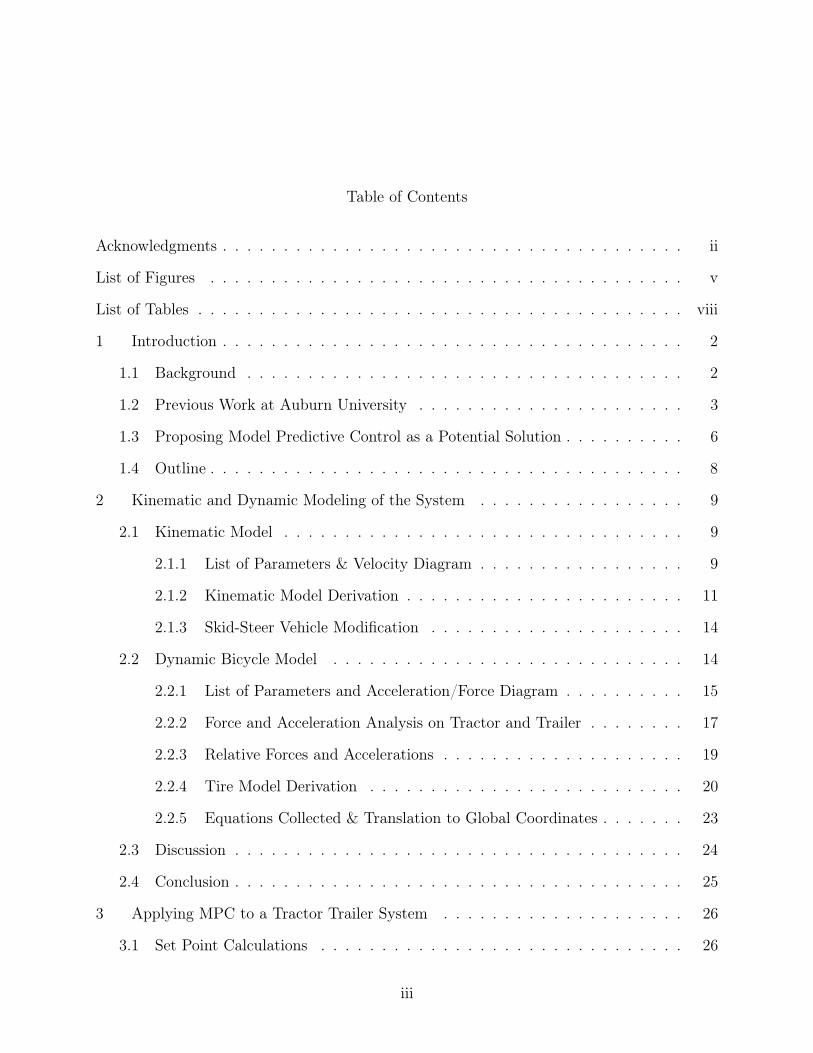
Table of Contents
Acknowledgments . . . . . . . . . . . . . . . . . . . . . . . . . . . . . . . . . . . . . . ii
List of Figures . . . . . . . . . . . . . . . . . . . . . . . . . . . . . . . . . . . . . . . v
List of Tables . . . . . . . . . . . . . . . . . . . . . . . . . . . . . . . . . . . . . . . . viii
1 Introduction . . . . . . . . . . . . . . . . . . . . . . . . . . . . . . . . . . . . . . 2
1.1 Background . . . . . . . . . . . . . . . . . . . . . . . . . . . . . . . . . . . . 2
1.2 Previous Work at Auburn University . . . . . . . . . . . . . . . . . . . . . . 3
1.3 Proposing Model Predictive Control as a Potential Solution . . . . . . . . . . 6
1.4 Outline . . . . . . . . . . . . . . . . . . . . . . . . . . . . . . . . . . . . . . . 8
2 Kinematic and Dynamic Modeling of the System . . . . . . . . . . . . . . . . . 9
2.1 Kinematic Model . . . . . . . . . . . . . . . . . . . . . . . . . . . . . . . . . 9
2.1.1 List of Parameters & Velocity Diagram . . . . . . . . . . . . . . . . . 9
2.1.2 Kinematic Model Derivation . . . . . . . . . . . . . . . . . . . . . . . 11
2.1.3 Skid-Steer Vehicle Modification . . . . . . . . . . . . . . . . . . . . . 14
2.2 Dynamic Bicycle Model . . . . . . . . . . . . . . . . . . . . . . . . . . . . . 14
2.2.1 List of Parameters and Acceleration/Force Diagram . . . . . . . . . . 15
2.2.2 Force and Acceleration Analysis on Tractor and Trailer . . . . . . . . 17
2.2.3 Relative Forces and Accelerations . . . . . . . . . . . . . . . . . . . . 19
2.2.4 Tire Model Derivation . . . . . . . . . . . . . . . . . . . . . . . . . . 20
2.2.5 Equations Collected & Translation to Global Coordinates . . . . . . . 23
2.3 Discussion . . . . . . . . . . . . . . . . . . . . . . . . . . . . . . . . . . . . . 24
2.4 Conclusion . . . . . . . . . . . . . . . . . . . . . . . . . . . . . . . . . . . . . 25
3 Applying MPC to a Tractor Trailer System . . . . . . . . . . . . . . . . . . . . 26
3.1 Set Point Calculations . . . . . . . . . . . . . . . . . . . . . . . . . . . . . . 26
iii

3.1.1 Initial Setup . . . . . . . . . . . . . . . . . . . . . . . . . . . . . . . . 27
3.1.2 Finding Minimum Cost Using Newton’s Method . . . . . . . . . . . . 32
3.1.3 Finding Minimum Cost using Golden Section Search . . . . . . . . . 34
3.2 Control Calculations . . . . . . . . . . . . . . . . . . . . . . . . . . . . . . . 38
3.2.1 Steering Motor Voltage Calculations for Front-Steering Tractor . . . . 38
3.3 Conclusion . . . . . . . . . . . . . . . . . . . . . . . . . . . . . . . . . . . . . 43
4 Computer Simulations and Live Application . . . . . . . . . . . . . . . . . . . . 45
4.1 Kubota RTV Simulation Results . . . . . . . . . . . . . . . . . . . . . . . . . 45
4.1.1 Kinematic Controller Model against Bicycle Plant Model . . . . . . . 45
4.1.2 Linearized Kinematic Controller Model against Nonlinear Kinematic
Plant Model . . . . . . . . . . . . . . . . . . . . . . . . . . . . . . . . 48
4.2 Segway Simulation Results . . . . . . . . . . . . . . . . . . . . . . . . . . . . 51
4.3 Segway Experimental Results . . . . . . . . . . . . . . . . . . . . . . . . . . 55
4.3.1 Controller Tuning . . . . . . . . . . . . . . . . . . . . . . . . . . . . . 59
4.3.2 Turn Rate Analysis . . . . . . . . . . . . . . . . . . . . . . . . . . . . 64
4.3.3 Applying the Scale Factor to the Input . . . . . . . . . . . . . . . . . 66
4.4 Conclusion . . . . . . . . . . . . . . . . . . . . . . . . . . . . . . . . . . . . . 69
5 Summary and Conclusion . . . . . . . . . . . . . . . . . . . . . . . . . . . . . . 70
A Model Predictive Control - A General Case . . . . . . . . . . . . . . . . . . . . . 72
B Bicycle Model State Equations, Separated by State Variable . . . . . . . . . . . 75
Bibliography . . . . . . . . . . . . . . . . . . . . . . . . . . . . . . . . . . . . . . . . 79
iv
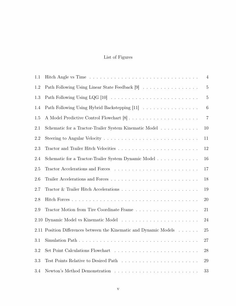
List of Figures
1.1 Hitch Angle vs Time . . . . . . . . . . . . . . . . . . . . . . . . . . . . . . . 4
1.2 Path Following Using Linear State Feedback [9] . . . . . . . . . . . . . . . . 5
1.3 Path Following Using LQG [10] . . . . . . . . . . . . . . . . . . . . . . . . . 5
1.4 Path Following Using Hybrid Backstepping [11] . . . . . . . . . . . . . . . . 6
1.5 A Model Predictive Control Flowchart [8] . . . . . . . . . . . . . . . . . . . . 7
2.1 Schematic for a Tractor-Trailer System Kinematic Model . . . . . . . . . . . 10
2.2 Steering to Angular Velocity . . . . . . . . . . . . . . . . . . . . . . . . . . . 11
2.3 Tractor and Trailer Hitch Velocities . . . . . . . . . . . . . . . . . . . . . . . 12
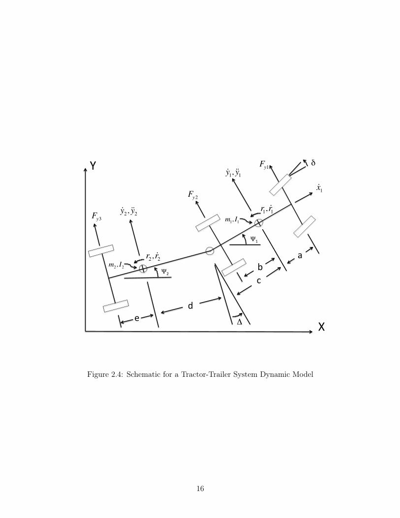
2.4 Schematic for a Tractor-Trailer System Dynamic Model . . . . . . . . . . . . 16
2.5 Tractor Accelerations and Forces . . . . . . . . . . . . . . . . . . . . . . . . 17
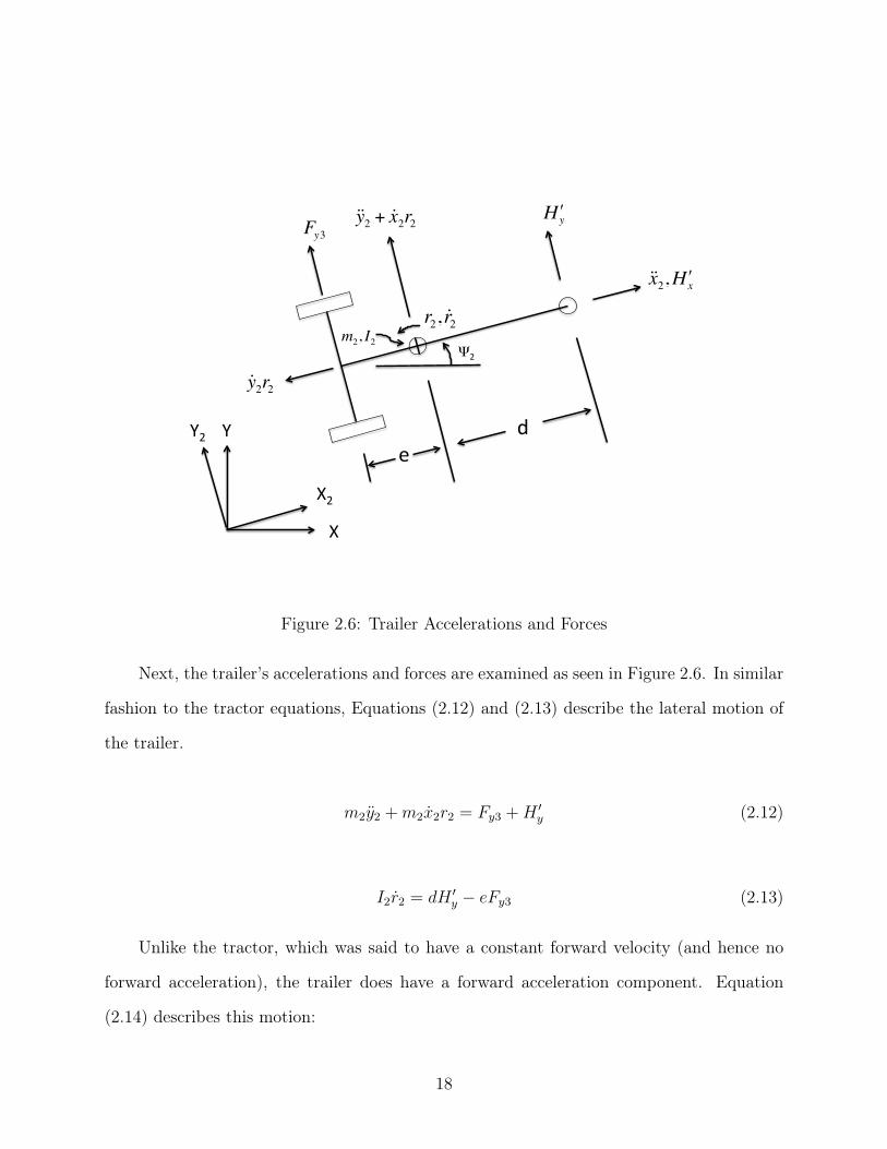
2.6 Trailer Accelerations and Forces . . . . . . . . . . . . . . . . . . . . . . . . . 18
2.7 Tractor & Trailer Hitch Accelerations . . . . . . . . . . . . . . . . . . . . . . 19
2.8 Hitch Forces . . . . . . . . . . . . . . . . . . . . . . . . . . . . . . . . . . . . 20
2.9 Tractor Motion from Tire Coordinate Frame . . . . . . . . . . . . . . . . . . 21
2.10 Dynamic Model vs Kinematic Model . . . . . . . . . . . . . . . . . . . . . . 24
2.11 Position Differences between the Kinematic and Dynamic Models . . . . . . 25
3.1 Simulation Path . . . . . . . . . . . . . . . . . . . . . . . . . . . . . . . . . . 27
3.2 Set Point Calculations Flowchart . . . . . . . . . . . . . . . . . . . . . . . . 28
3.3 Test Points Relative to Desired Path . . . . . . . . . . . . . . . . . . . . . . 29
3.4 Newton’s Method Demonstration . . . . . . . . . . . . . . . . . . . . . . . . 33
v

3.5 MPC Set Point Simulation . . . . . . . . . . . . . . . . . . . . . . . . . . . . 34
3.6 Newton’s Method Incompatibility . . . . . . . . . . . . . . . . . . . . . . . . 35
3.7 Golden Section Search . . . . . . . . . . . . . . . . . . . . . . . . . . . . . . 37
3.8 Steering Angle Set-Points . . . . . . . . . . . . . . . . . . . . . . . . . . . . 38
3.9 Armature Motor Model . . . . . . . . . . . . . . . . . . . . . . . . . . . . . . 39
3.10 Controlled Motor System . . . . . . . . . . . . . . . . . . . . . . . . . . . . . 39
3.11 Unwanted Oscillations . . . . . . . . . . . . . . . . . . . . . . . . . . . . . . 40
3.12 Proportional Control . . . . . . . . . . . . . . . . . . . . . . . . . . . . . . . 41
3.13 Proportional-Integral Control . . . . . . . . . . . . . . . . . . . . . . . . . . 41
3.14 Steer Angle Controlled . . . . . . . . . . . . . . . . . . . . . . . . . . . . . . 42
3.15 Voltage Across Motor vs Time (using PI control) . . . . . . . . . . . . . . . 42
3.16 Motor Response to Step Input with Varying Derivative Control Values . . . 43
3.17 Voltage Across Motor vs Time (using PID control) . . . . . . . . . . . . . . 44
4.1 MPC with Model Error . . . . . . . . . . . . . . . . . . . . . . . . . . . . . . 46
4.2 Deviation with High Model Error . . . . . . . . . . . . . . . . . . . . . . . . 46
4.3 Deviation with Low Model Error . . . . . . . . . . . . . . . . . . . . . . . . 47
4.4 Wide S-curve Path Following . . . . . . . . . . . . . . . . . . . . . . . . . . 48
4.5 Path Following Using Nonlinear Control Model . . . . . . . . . . . . . . . . 49
4.6 Path Following Using Linear Control Model . . . . . . . . . . . . . . . . . . 49
4.7 15m Radius S-curve . . . . . . . . . . . . . . . . . . . . . . . . . . . . . . . . 50
4.8 Path Following Using Nonlinear Control Model (15m radius) . . . . . . . . . 50
4.9 Path Following Using Linear Control Model (15m radius) . . . . . . . . . . . 51
4.10 Segway Simulator [18] . . . . . . . . . . . . . . . . . . . . . . . . . . . . . . 52
4.11 Segway & Trailer Positions, Simulated . . . . . . . . . . . . . . . . . . . . . 53
4.12 Path Following Error, Simulated . . . . . . . . . . . . . . . . . . . . . . . . . 54
vi
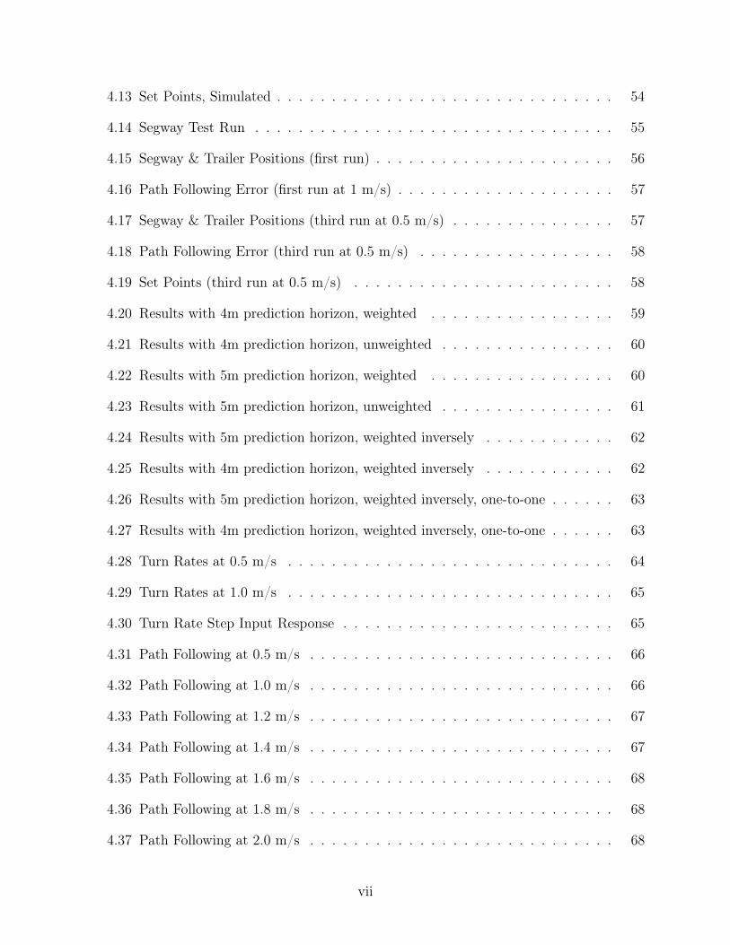
4.13 Set Points, Simulated . . . . . . . . . . . . . . . . . . . . . . . . . . . . . . . 54
4.14 Segway Test Run . . . . . . . . . . . . . . . . . . . . . . . . . . . . . . . . . 55
4.15 Segway & Trailer Positions (first run) . . . . . . . . . . . . . . . . . . . . . . 56
4.16 Path Following Error (first run at 1 m/s) . . . . . . . . . . . . . . . . . . . . 57
4.17 Segway & Trailer Positions (third run at 0.5 m/s) . . . . . . . . . . . . . . . 57
4.18 Path Following Error (third run at 0.5 m/s) . . . . . . . . . . . . . . . . . . 58
4.19 Set Points (third run at 0.5 m/s) . . . . . . . . . . . . . . . . . . . . . . . . 58
4.20 Results with 4m prediction horizon, weighted . . . . . . . . . . . . . . . . . 59
4.21 Results with 4m prediction horizon, unweighted . . . . . . . . . . . . . . . . 60
4.22 Results with 5m prediction horizon, weighted . . . . . . . . . . . . . . . . . 60
4.23 Results with 5m prediction horizon, unweighted . . . . . . . . . . . . . . . . 61
4.24 Results with 5m prediction horizon, weighted inversely . . . . . . . . . . . . 62
4.25 Results with 4m prediction horizon, weighted inversely . . . . . . . . . . . . 62
4.26 Results with 5m prediction horizon, weighted inversely, one-to-one . . . . . . 63
4.27 Results with 4m prediction horizon, weighted inversely, one-to-one . . . . . . 63
4.28 Turn Rates at 0.5 m/s . . . . . . . . . . . . . . . . . . . . . . . . . . . . . . 64
4.29 Turn Rates at 1.0 m/s . . . . . . . . . . . . . . . . . . . . . . . . . . . . . . 65
4.30 Turn Rate Step Input Response . . . . . . . . . . . . . . . . . . . . . . . . . 65
4.31 Path Following at 0.5 m/s . . . . . . . . . . . . . . . . . . . . . . . . . . . . 66
4.32 Path Following at 1.0 m/s . . . . . . . . . . . . . . . . . . . . . . . . . . . . 66
4.33 Path Following at 1.2 m/s . . . . . . . . . . . . . . . . . . . . . . . . . . . . 67
4.34 Path Following at 1.4 m/s . . . . . . . . . . . . . . . . . . . . . . . . . . . . 67
4.35 Path Following at 1.6 m/s . . . . . . . . . . . . . . . . . . . . . . . . . . . . 68
4.36 Path Following at 1.8 m/s . . . . . . . . . . . . . . . . . . . . . . . . . . . . 68
4.37 Path Following at 2.0 m/s . . . . . . . . . . . . . . . . . . . . . . . . . . . . 68
vii

List of Tables
2.1 List of Tractor-Trailer System Parameters (kinematic model) . . . . . . . . . 11
2.2 List of Tractor-Trailer System Parameters (dynamic model) . . . . . . . . . 15
4.1 List of Segway & Trailer Simulation Parameters (kinematic model) . . . . . 52
4.2 List of Segway & Trailer Live Parameters (kinematic model) . . . . . . . . . 55
4.3 Scale Factors . . . . . . . . . . . . . . . . . . . . . . . . . . . . . . . . . . . 59
4.4 Inverted Scale Factors . . . . . . . . . . . . . . . . . . . . . . . . . . . . . . 61
4.5 Inverted Scale Factors, One-to-One . . . . . . . . . . . . . . . . . . . . . . . 63
viii

List of Symbols
� Angle Difference between Tractor and Trailer ( 1
� 2
)
� Front Tire Steering Angle of Tractor
x1
Forward Velocity of Tractor
x2
, x2
Forward Velocity and Acceleration of Trailer
y1
, y1
Lateral Velocity and Acceleration of Tractor
y2
, y2
Lateral Velocity and Acceleration of Trailer
1
, r1
, r1
Heading, Angular Velocity, and Angular Acceleration of Tractor
2
, r2
, r2
Heading, Angular Velocity, and Angular Acceleration of Trailer
✓pathj Angle between Trailer’s current heading and closest path point (when finding cost)
✓predj Angle between Trailer’s current heading and j-th Prediction Point (when finding cost)
a Length from Tractor GPS (kinematic model) or CG (dynamic model) to front tire
b Length from Tractor GPS (kinematic model) or CG (dynamic model) to back tire
c Length from Tractor GPS (kinematic model) or CG (dynamic model) to hitch
C1
Cornering Coefficient of the Front Tractor Tire
C2
Cornering Coefficient of the Back Tractor Tire
C3
Cornering Coefficient of the Trailer Tire
d Length from Trailer GPS (kinematic model) or CG (dynamic model) to hitch
ix
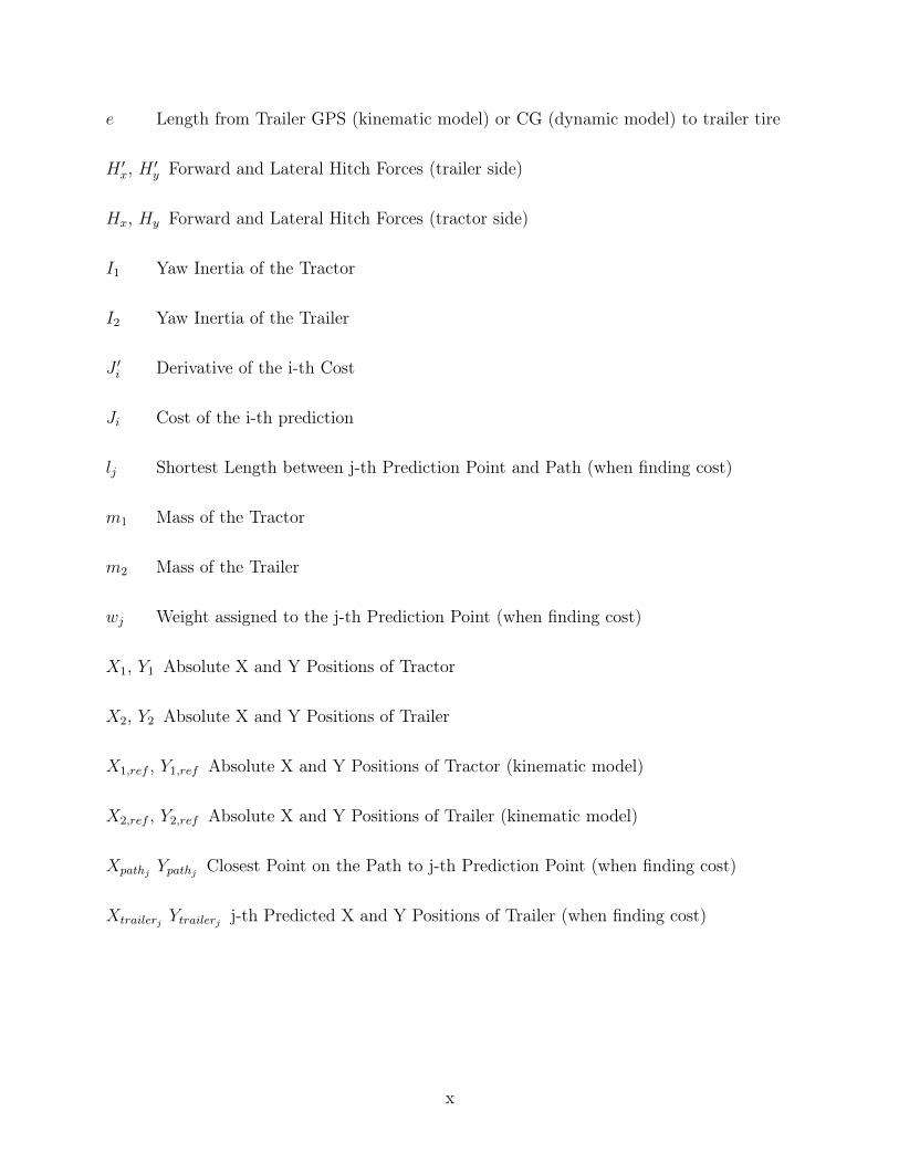
e Length from Trailer GPS (kinematic model) or CG (dynamic model) to trailer tire
H 0x
, H 0y
Forward and Lateral Hitch Forces (trailer side)
Hx
, Hy
Forward and Lateral Hitch Forces (tractor side)
I1
Yaw Inertia of the Tractor
I2
Yaw Inertia of the Trailer
J 0i
Derivative of the i-th Cost
Ji
Cost of the i-th prediction
lj
Shortest Length between j-th Prediction Point and Path (when finding cost)
m1
Mass of the Tractor
m2
Mass of the Trailer
wj
Weight assigned to the j-th Prediction Point (when finding cost)
X1
, Y1
Absolute X and Y Positions of Tractor
X2
, Y2
Absolute X and Y Positions of Trailer
X1,ref
, Y1,ref
Absolute X and Y Positions of Tractor (kinematic model)
X2,ref
, Y2,ref
Absolute X and Y Positions of Trailer (kinematic model)
Xpathj Y
pathj Closest Point on the Path to j-th Prediction Point (when finding cost)
Xtrailerj Y
trailerj j-th Predicted X and Y Positions of Trailer (when finding cost)
x

Abstract
This thesis presents an effort to improve the path following reliability of a tractor-trailer
system by using a non-linear Model Predictive Control (MPC) approach. The proposed
method allows an autonomous mobile robot to make informed control decisions based on
anticipating changes in the path conditions, rather than reacting to them, which could
potentially reduce path following error on turns.
Using a non-linear tractor-trailer model, the controller takes the tractor’s measured
position and heading, as well as information about the path geometry in front of it, and
it determines the optimal steer angle. Then, in the case of an Ackerman-steered vehicle, a
secondary algorithm takes the desired steer angle and calculates the amount of voltage to
apply to the steering wheel motor to achieve the steer angle. In comparison, a differential-
steered, or skid-steered vehicle takes the set point (given as a turn rate in radians per second)
and computes the voltages to the traction motors internally.
In the MATLAB simulation study, the controller algorithm is capable of guiding a 2-
1/2 meter long trailer around a 5-meter radius turn, when towed by a four wheel drive
off-road utility vehicle, with a maximum error of 8.5 centimeters. These results are highly
idealized, however. Adding sensor noise and process noise in simulation increases the error,
and inherent sensor bias and latency during the live run increases the error substantially.
From the experimental results, it is concluded that non-linear MPC has the potential
to improve the reliability of the path following of a robot and trailer system. In order to
fully reap the benefits of non-linear MPC however, the model has to be accurate, and the
computer has to be fast enough to compute predictions from the model in real-time.
1
Chapter 1
Introduction
Model Predictive Control (MPC) is a relatively new control method, first practiced by
Shell Oil, which determines an optimal input, called a set point, and then guides the system
to that set point. It is a control technique that is commonly used in the oil industry, as well
as other applications in chemical engineering. With advancements in computing power, en-
gineers have begun exploring the usage of MPC to other applications, including autonomous
vehicle control. However, due to the computational expense of MPC, especially when a
nonlinear model is used, most vehicular applications are limited to low-speed operation [1].
For many off-road vehicle applications however, low-speed operation is the norm. In
agriculture, tractor-trailer systems are used to spread seed, fertilizer and top soil. In the case
of the Department of Defense, a tractor pulls a fiberglass trailer that carries metal sensors
to scan the ground for unexploded ordnance, which is further explained in [2]. Despite the
computational expense of MPC, these applications involve process that are slow enough for
MPC to produce good results.
1.1 Background
Auburn University, with the support of the U.S. Army Corps of Engineers, has been
researching ways to control off-road tractor-trailer systems for conducting geophysical sur-
veys, with the trailer being the object of interest for control. A geophysical survey involves
a scan of a given area in search of metal objects in the ground [9].
In an effort to streamline the U.S. Military, the Department of Defense (DOD) has
initiated numerous military base closures around the United States. Many of these bases
contained training sites for tactical strategies that are less commonly used in modern military
2
operations. According to [3], the DOD closed or realigned over 800 defense locations and
relocated over 125,000 personnel since 2005, in an operation called Base Realignment and
Closure (BRAC). When a base closes, the land is sold to private developers. However, there
are legitimate safety concerns regarding unexploded ordnance (UXO) still remaining on plots
of land that used to be training sites.
To ensure that a questionable field is safe, the Army Corps of Engineers conducts geo-
physical surveys to look for potential UXO. While there have been no recorded incidents of
injuries or fatalities during these surveys due to accidental discharge, the risk is still a con-
cern. This is why the Army Corps of Engineers has tasked Auburn University in developing
an unmanned robot vehicle that would carry out the task of searching for UXO. Auburn has
since used a setup consisting of a GPS guided trailer made of fiberglass, towed by a tractor
[5], which would allow the scanning of the ground for metal objects without interference
from the metal inside the tractor.
1.2 Previous Work at Auburn University
Previously, linear state feedback controllers [9], LQG controllers [10], and hybrid back-
stepping controllers [11] were used in the guidance of the surveying system. In all cases,
these control methods work very well in guiding the trailer to the path, as long as the path
is straight. However, due to the complexity of tractor-trailer system dynamics, keeping the
trailer on the path becomes much more difficult when going around turns. The most accu-
rate controller found so far was the linear state feedback controller, which had a maximum
recovery error of 20.4cm [9]. Conversely, the hybrid backstepping controller had maximum
errors of up to 40cm [11], and the LQG controller had maximum errors of around 44cm
[10]. Both authors conclude, however, that these errors might be improved by fine-tuning
the gains.
This thesis proposes, on the other hand, that the biggest source of error is the non-
linearity of a tractor-trailer hitch connection. According to [14], when the angle between
3

Figure 1.1: Hitch Angle vs Time
the tractor and the trailer exceeds 7°, linearized tractor-trailer models become less accurate.
Figure 1.1 shows a time plot of the hitch angle, where the maximum hitch angle reaches
47.8° as a simulated tractor-trailer system navigates an S-curve with turn radii of 5 meters.
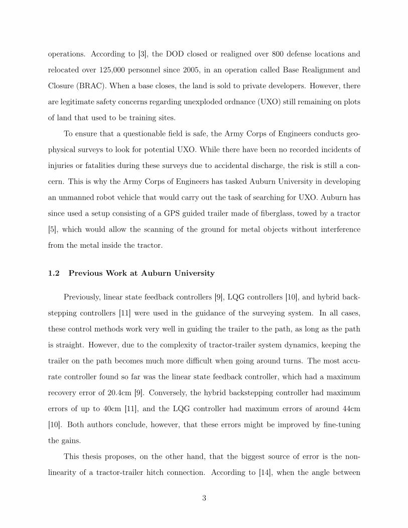
The biggest issue during a geophysical survey is recovering out of a turn. As seen
in Figure 1.2, the robot overshoots the beginning of the straight sections of the desired
path, and then it corrects itself. In the case of Figure 1.3, the robot overcompensates and
undergoes an oscillatory correction maneuver to return to the desired path. Finally, in Figure
1.4, the robot does a combination of overshooting the straight section reentries, as well as
overcompensating for errors. With these errors, the ground scanners on the trailer could
potentially miss locations on the ground that contain critical information.
In each of the afore-mentioned works, the robot follows what is known as a “Dubins
path.” According to Lester E. Dubins, the shortest path between two oriented points consists
of straight lines and turns of constant radii [4]. However, dynamic constraints make it
infeasible for a non-holonomic trailer to follow a path perfectly where the curvature changes
instantaneously. One way to address this problem is to design paths with clothoid turns,
4
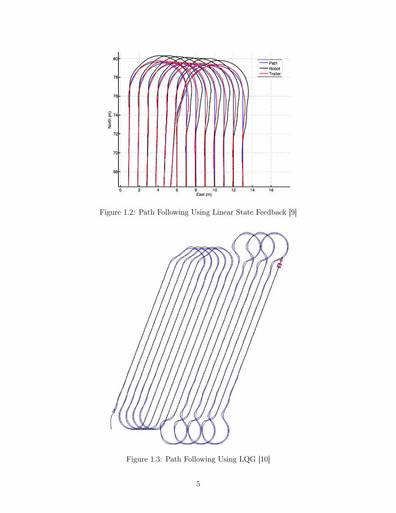
Figure 1.2: Path Following Using Linear State Feedback [9]
Figure 1.3: Path Following Using LQG [10]
5

Figure 1.4: Path Following Using Hybrid Backstepping [11]
as studied in [6]. A clothoid is an arc where the curvature changes linearly, as opposed
to instantaneously. They are commonly used in highway and railway design, and several
clothoid computation algorithms exist, such as the one introduced in [7]. For each of the
experiments done in this thesis, however, a constant radius turn will be used. This will
force an error into the system intentionally, and it would allow the controller’s recovery
performance to be measured.
1.3 Proposing Model Predictive Control as a Potential Solution
The goal of this research is to develop a control algorithm that will improve the guidance
of a trailer to a desired path during and after making a turn. Unlike the controllers previ-
ously used at Auburn University which choose guidance inputs based on the trailer’s current
position relative to the path, this thesis proposes designing a model predictive controller that
chooses guidance inputs based on where the trailer is predicted to go, based upon a model.
This is similar to the way a human drives a car, as a human subconsciously predicts where
6

Figure 1.5: A Model Predictive Control Flowchart [8]
his or her car is going to go given a forward and steering input, and then the human adjusts
the forward and steering controls of the car accordingly.
Of course, it is fair to ask the question of whether or not a computer can make model
calculations fast enough to determine the optimal control inputs. After all, if a computer
takes too long to predict an optimal solution, the control system becomes useless. Also, if
the model is oversimplified, a model predictive controller’s performance would be no better
than a classical controller. For this application, however, the robot moves at a forward speed
of 1 meter per second. Because of the low speed of the system, inertial properties as well
as tire slip properties of the tractor and trailer will be ignored, and a simplified kinematic
tractor-trailer model will be used, making the nonlinear MPC calculations feasible.
In general, MPC follows an algorithm depicted by the flowchart in Figure 1.5. First,
the controller makes a prediction, choosing a particular steer angle. Then, using a model of
the system, the controller looks at where the trailer will go if the robot uses that steer angle.
It will then compare the result to the desired path. If the result does not meet tolerance
specifications, it will make another prediction. Otherwise, the controller will use this steer
angle (now called a set-point) as a target angle to move the steering wheel to. The controller
then determines the voltage into the steering motor by making control calculations, and it
feeds that voltage into the motor. The controller also runs the input back through the model
and compares the result from the process’s feedback sensors (in this case, a GPS receiver).
7
1.4 Outline
This thesis introduces a numerical approach to a non-linear feedforward control problem,
and it stresses real-time feasibility. It is necessary for the control system to determine
inputs quickly, while maintaining a high degree of accuracy. Two tractor-trailer models
are presented in Chapter 2. The first, a 4th-order kinematic model, is a standard control
model that is currently being used at Auburn University. The second model, a 9th-order
bicycle model, has not been used at Auburn yet, due to its complexity and difficulty for
a computer to numerically compute in real-time. Chapter 3 presents the numerical MPC
method responsible for choosing the appropriate set points, and it shows how these set points
can be achieved through classical control method design. Chapter 4 includes results from
computer simulations with the two competing tractor-trailer models described in Chapter
2, as well as results from an experimental run on a Segway RMP 400. Finally, Chapter 5
presents conclusions from the results of this work and proposes future work.
8
Chapter 2
Kinematic and Dynamic Modeling of the System
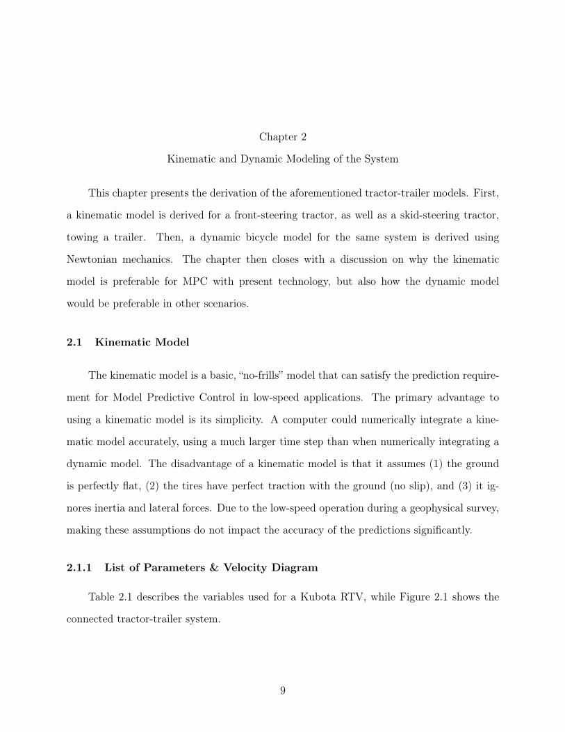
This chapter presents the derivation of the aforementioned tractor-trailer models. First,
a kinematic model is derived for a front-steering tractor, as well as a skid-steering tractor,
towing a trailer. Then, a dynamic bicycle model for the same system is derived using
Newtonian mechanics. The chapter then closes with a discussion on why the kinematic
model is preferable for MPC with present technology, but also how the dynamic model
would be preferable in other scenarios.
2.1 Kinematic Model
The kinematic model is a basic, “no-frills” model that can satisfy the prediction require-
ment for Model Predictive Control in low-speed applications. The primary advantage to
using a kinematic model is its simplicity. A computer could numerically integrate a kine-
matic model accurately, using a much larger time step than when numerically integrating a
dynamic model. The disadvantage of a kinematic model is that it assumes (1) the ground
is perfectly flat, (2) the tires have perfect traction with the ground (no slip), and (3) it ig-
nores inertia and lateral forces. Due to the low-speed operation during a geophysical survey,
making these assumptions do not impact the accuracy of the predictions significantly.
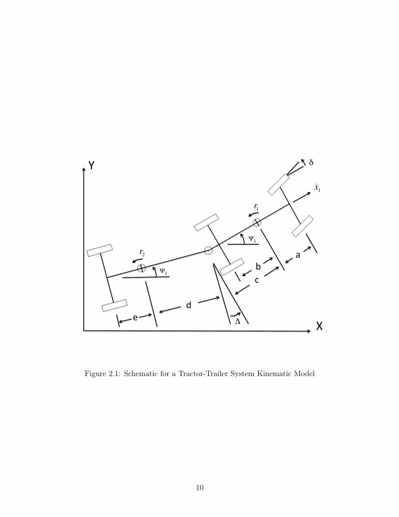
2.1.1 List of Parameters & Velocity Diagram
Table 2.1 describes the variables used for a Kubota RTV, while Figure 2.1 shows the
connected tractor-trailer system.
9
X"
Y"
Ψ2"
Ψ1"
r1
r2
c"
a"b"
de" Δ"
&x1
δ"
Figure 2.1: Schematic for a Tractor-Trailer System Kinematic Model
10
Parameter Description Value (if constant)X
1,ref
Absolute X Position of Tractor variableY1,ref
Absolute Y Position of Tractor variableX
2,ref
Absolute X Position of Trailer variableY2,ref
Absolute Y Position of Trailer variableX
1
Absolute X Position of Tractor (back axle) variableY1
Absolute Y Position of Tractor (back axle) variablex1
Forward Velocity of the Tractor 1 m/s
1
, r1
Heading and Angular Velocity of Tractor variable
2
, r2
Heading and Angular Velocity of Trailer variable� Front Tire Steering Angle of Tractor variable� Angle Difference between Tractor and Trailer (
1
� 2
)
1
� 2
a Length from Tractor GPS receiver to center of front tire 0.75 mb Length from Tractor GPS receiver to center of back tire 1.21 mc Length from Tractor GPS receiver to hitch 1.74 md Length from Trailer GPS receiver to hitch 3.0 me Length from Trailer GPS receiver to trailer tire 1.0 m
Table 2.1: List of Tractor-Trailer System Parameters (kinematic model)
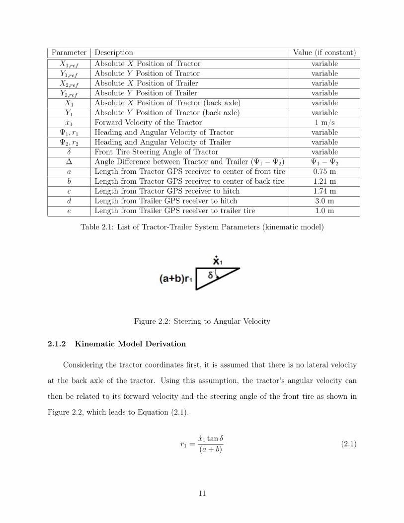
Figure 2.2: Steering to Angular Velocity
2.1.2 Kinematic Model Derivation
Considering the tractor coordinates first, it is assumed that there is no lateral velocity
at the back axle of the tractor. Using this assumption, the tractor’s angular velocity can
then be related to its forward velocity and the steering angle of the front tire as shown in
Figure 2.2, which leads to Equation (2.1).
r1
=
x1
tan �
(a+ b)(2.1)
11
r2d
e#
d + e( )r2
&x2
r1
c#
a#b#
c− b( )r1
&x1
X2#
X1#
Y2#Y1#
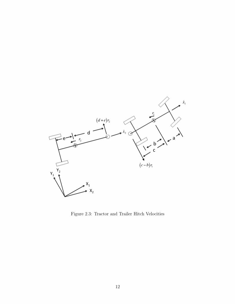
Figure 2.3: Tractor and Trailer Hitch Velocities
12
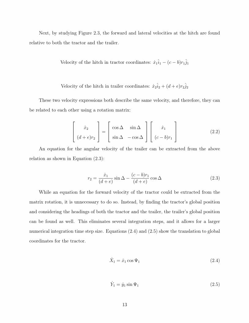
Next, by studying Figure 2.3, the forward and lateral velocities at the hitch are found
relative to both the tractor and the trailer.
Velocity of the hitch in tractor coordinates: x1
ˆi1
� (c� b)r1
ˆj1
Velocity of the hitch in trailer coordinates: x2
ˆi2
+ (d+ e)r2
ˆj2
These two velocity expressions both describe the same velocity, and therefore, they can
be related to each other using a rotation matrix:
2
64x2
(d+ e)r2
3
75 =
2
64cos� sin�
sin� � cos�
3
75
2
64x1
(c� b)r1
3
75 (2.2)
An equation for the angular velocity of the trailer can be extracted from the above
relation as shown in Equation (2.3):
r2
=
x1
(d+ e)sin�� (c� b)r
1
(d+ e)cos� (2.3)
While an equation for the forward velocity of the tractor could be extracted from the
matrix rotation, it is unnecessary to do so. Instead, by finding the tractor’s global position
and considering the headings of both the tractor and the trailer, the trailer’s global position
can be found as well. This eliminates several integration steps, and it allows for a larger
numerical integration time step size. Equations (2.4) and (2.5) show the translation to global
coordinates for the tractor.
˙X1
= x1
cos
1
(2.4)
˙Y1
= y1
sin
1
(2.5)
13

To summarize the derivation so far, Equations (2.1), (2.4), and (2.5) give the position
and heading of the back axle of the tractor, while Equation (2.3) gives the angular velocity
of the trailer. Now, some kinematic relations are considered to locate the points of interest
(i.e. the GPS receivers) on both the tractor and the trailer. Equations (2.6) and (2.7) give
the antenna location on the tractor:
X1,ref
= X1
+ b cos 1
(2.6)
Y1,ref
= Y1
+ b sin 1
(2.7)
Finally, the trailer’s GPS receiver location can be calculated using the following Equa-
tions (2.8) and (2.9):
X2,ref
= X1,ref
� c cos 1
� d cos 2
(2.8)
Y2,ref
= Y1,ref
� c sin 1
� d sin 2
(2.9)
2.1.3 Skid-Steer Vehicle Modification
Many skid-steer vehicles, such as the Segway Robotics Mobility Platform (RMP) 400,
have an existing steering control system that only requires an angular velocity input, re-
moving the need for Equation (2.1). However, there is often a time delay between the
angular velocity input, and when the robot reaches that angular velocity. The design of a
compensator for this delay will be addressed in Chapter 3.
2.2 Dynamic Bicycle Model
The dynamic bicycle model introduces the possibility of adding exterior input forces
to the model, such as bumps and dips in the ground. The major difference in the model
14

Parameter Description ValueX
1
Absolute X Position of Tractor (center of gravity) variableY1
Absolute Y Position of Tractor (center of gravity) variableX
2
Absolute X Position of Trailer (center of gravity) variableY2
Absolute Y Position of Trailer (center of gravity) variablex1
Forward Velocity of Tractor 1 m/sy1,
y1
Lateral Velocity and Acceleration of Tractor variablex2
, x2
Forward Velocity and Acceleration of Trailer variabley2
, y2
Lateral Velocity and Acceleration of the Trailer variable
1
, r1
, r1
Heading, Angular Velocity, and Angular Acceleration of Tractor variable
2
, r2
, r2
Heading, Angular Velocity, and Angular Acceleration of Trailer variableH
x
, Hy
Forward and Lateral Hitch Forces (tractor side) variableH 0
x
, H 0y
Forward and Lateral Hitch Forces (trailer side) variable� Front Tire Steering Angle of Tractor variable� Angle Difference between Tractor and Trailer (
1
� 2
)
1
� 2
a Length from Tractor CG to center of front tire 0.75 mb Length from Tractor CG to center of back tire 1.21 mc Length from Tractor CG to hitch 1.74 md Length from Trailer CG to hitch 3.0 me Length from Trailer CG to trailer tire 1.0 mm
1
Mass of the Tractor 1225 kgI1
Yaw Inertia of the Tractor m1
· a · bm
2
Mass of the Trailer 30 kgI2
Yaw Inertia of the Trailer m2
· d · eC
1
Cornering Coefficient of the Front Tractor Tire 80 ·m1
C2
Cornering Coefficient of the Back Tractor Tire 80 ·m1
C3
Cornering Coefficient of the Trailer Tire 80 ·m2
Table 2.2: List of Tractor-Trailer System Parameters (dynamic model)
assumptions is that the tires no longer have perfect traction with the ground, and they have
to push against the ground in order to control a vehicle’s direction. These advantages come
at a cost, however, as the numerical computation requires a significantly smaller time step
size than the kinematic model.
2.2.1 List of Parameters and Acceleration/Force Diagram
Table 2.2 describes the variables used for a Kubota RTV, while Figure 2.4 shows the
connected tractor-trailer system.
15
X"
Y"
Ψ2"
Ψ1"
r1, &r1
r2, &r2
c"
a"b"
de" Δ"
&y1, &&y1
&y2, &&y2
Fy1
Fy2
Fy3
&x1
δ"
m2, I2
m1, I1
Figure 2.4: Schematic for a Tractor-Trailer System Dynamic Model
16

X"
Y"
X1"
Y1"
Ψ1"
&r1
c"
a"b"
&&y1 + &x1r1Fy1
Fy2
m1, I1
δ"
Hy
&y1r1,Hx
Figure 2.5: Tractor Accelerations and Forces
2.2.2 Force and Acceleration Analysis on Tractor and Trailer
As seen in Figure 2.5, the tractor has three lateral forces acting on it: two produced
by the tires, and a lateral force produced at the hitch. There are two lateral acceleration
components influenced by these forces – a lateral perturbed acceleration y1
, and a centripetal
acceleration x1
r1
. These forces and accelerations relate as described by Equations (2.10) and
(2.11), using Newtonian mechanics.
m1
y1
+m1
x1
r1
= Fy1
+ Fy2
�Hy
(2.10)
I1
r1
= aFy1
� bFy2
+ cHy
(2.11)
17
X"
Y"
X2"
Y2"
Ψ2"
r2, &r2
de"
&&y2 + &x2r2Fy3
m2, I2
!Hy
&&x2, !Hx
&y2r2
Figure 2.6: Trailer Accelerations and Forces
Next, the trailer’s accelerations and forces are examined as seen in Figure 2.6. In similar
fashion to the tractor equations, Equations (2.12) and (2.13) describe the lateral motion of
the trailer.
m2
y2
+m2
x2
r2
= Fy3
+H 0y
(2.12)
I2
r2
= dH 0y
� eFy3
(2.13)
Unlike the tractor, which was said to have a constant forward velocity (and hence no
forward acceleration), the trailer does have a forward acceleration component. Equation
(2.14) describes this motion:
18

r1, &r1
c"
a"b"
&&y1 + &x1r1 − c&r1
&y1r1 − cr12
r2, &r2d
e"
&&y2 + &x2r2 + d&r2
&&x2 − &y2r2 − dr22
Figure 2.7: Tractor & Trailer Hitch Accelerations
m2
x2
�m2
y2
r2
= H 0x
(2.14)
2.2.3 Relative Forces and Accelerations
To relate the dynamic tractor and trailer models, similarly to the kinematic model, the
accelerations at the hitch can be determined with respect to both the tractor and the trailer
separately (see Figure 2.7), so they can be related using a rotation matrix (Equation (2.15)).
2
64x2
� (y2
r2
+ dr22
)
y2
+ x2
r2
+ dr2
3
75 =
2
64cos� � sin�
sin� cos�
3
75
2
64� (y
1
r1
� cr21
)
y1
+ x1
r1
� cr1
3
75 (2.15)
Using the same rotation matrix as Equation (2.15), Equation (2.16) relates the forces.
Note that by Newton’s Third Law, the force acting on the hitch from the perspective of the
19

c"
a"b"
Hy
Hx
de" !Hy
!Hx
Figure 2.8: Hitch Forces
tractor has to be equal and opposite to the force acting on the hitch from the perspective of
the trailer, as shown in Figure 2.8.
2
64H 0
x
H 0y
3
75 =
2
64cos� � sin�
sin� cos�
3
75
2
64H
x
Hy
3
75 (2.16)
2.2.4 Tire Model Derivation
Historically, tires have been difficult for engineers to model accurately. In most cases,
tire models are derived experimentally, as opposed to theoretically. For this model, however,
a somewhat non-intuitive approach called the “slip angle” model is used. The slip angle
concept does not imply skidding, but instead implies that as tires roll and experience a
lateral force, some portions of the tire begin to slip from their point of contact with the
20

Ψ1"
r1
c#
a#b#
&y1,tire &x1,tire
m1, I1
δ"
Hy
&x1β"
&y1
X1#
X1,(re#
Y1#Y1,(re#
Figure 2.9: Tractor Motion from Tire Coordinate Frame
ground, while other portions of the tire are still essentially “locked” to the ground by static
friction. For a more comprehensive description of the slip angle concept, refer to [12].
When a vehicle is traveling straight, there is virtually no difference between a vehi-
cle’s velocity and a tire’s velocity. However, if a perturbation is introduced in the vehicle’s
movement, the tire will react based on its motion relative to the vehicle.
Figure 2.9 shows an exaggeration of a vehicle’s perturbed motion from the coordinate
frame of the tire. For the following calculations, x will be the tire’s in-line rolling velocity,
y will be the tire’s lateral velocity, and will be the angle difference between the vehicle’s
forward motion and its lateral motion.
From Figure 2.9, the motion of the rear tractor tire can be related to the motion of the
vehicle as shown in Equations (2.17), (2.18), and (2.19).
21
�1
= arctan
✓�y
1
x1
◆(2.17)
x = x1
cos �1
+ y1
sin �1
(2.18)
y = �x1
sin �1
+ y1
cos �1
� br1
(2.19)
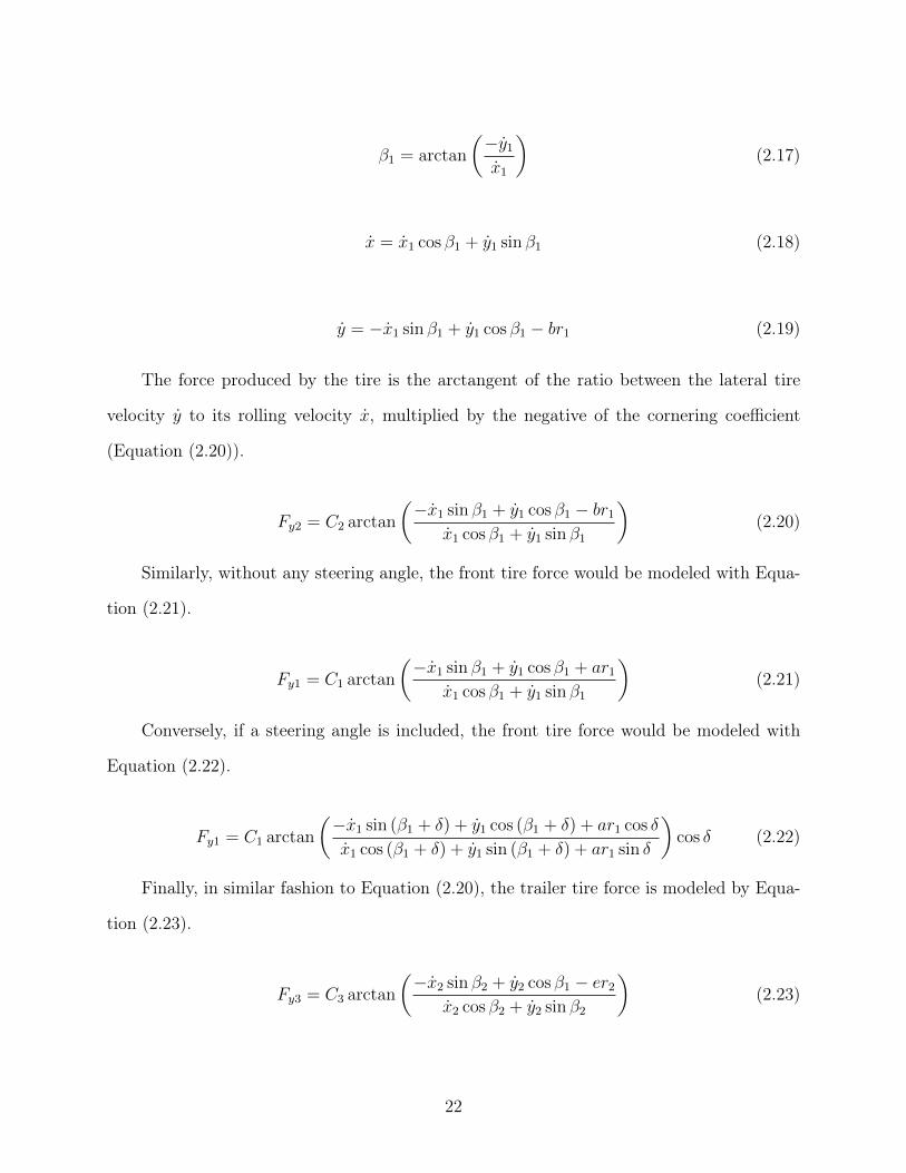
The force produced by the tire is the arctangent of the ratio between the lateral tire
velocity y to its rolling velocity x, multiplied by the negative of the cornering coefficient
(Equation (2.20)).
Fy2
= C2
arctan
✓�x
1
sin �1
+ y1
cos �1
� br1
x1
cos �1
+ y1
sin �1
◆(2.20)
Similarly, without any steering angle, the front tire force would be modeled with Equa-
tion (2.21).
Fy1
= C1
arctan
✓�x
1
sin �1
+ y1
cos �1
+ ar1
x1
cos �1
+ y1
sin �1
◆(2.21)
Conversely, if a steering angle is included, the front tire force would be modeled with
Equation (2.22).
Fy1
= C1
arctan
✓�x
1
sin (�1
+ �) + y1
cos (�1
+ �) + ar1
cos �
x1
cos (�1
+ �) + y1
sin (�1
+ �) + ar1
sin �
◆cos � (2.22)
Finally, in similar fashion to Equation (2.20), the trailer tire force is modeled by Equa-
tion (2.23).
Fy3
= C3
arctan
✓�x
2
sin �2
+ y2
cos �1
� er2
x2
cos �2
+ y2
sin �2
◆(2.23)
22
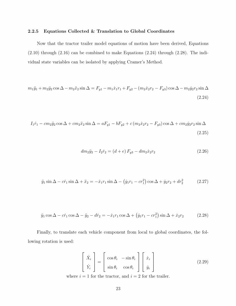
2.2.5 Equations Collected & Translation to Global Coordinates
Now that the tractor trailer model equations of motion have been derived, Equations
(2.10) through (2.16) can be combined to make Equations (2.24) through (2.28). The indi-
vidual state variables can be isolated by applying Cramer’s Method.
m1
y1
+m2
y2
cos��m2
x2
sin� = Fy1
�m1
x1
r1
+Fy2
� (m2
x2
r2
� Fy3
) cos��m2
y2
r2
sin�
(2.24)
I1
r1
� cm2
y2
cos�+ cm2
x2
sin� = aFy1
� bFy2
+ c (m2
x2
r2
� Fy3
) cos�+ cm2
y2
r2
sin�
(2.25)
dm2
y2
� I2
r2
= (d+ e)Fy3
� dm2
x2
r2
(2.26)
y1
sin�� cr1
sin�+ x2
= �x1
r1
sin���y1
r1
� cr21
�cos�+ y
2
r2
+ dr22
(2.27)
y1
cos�� cr1
cos�� y2
� dr2
= �x1
r1
cos�+
�y1
r1
� cr21
�sin�+ x
2
r2
(2.28)
Finally, to translate each vehicle component from local to global coordinates, the fol-
lowing rotation is used:
2
64˙Xi
˙Yi
3
75 =
2
64cos ✓
i
� sin ✓i
sin ✓i
cos ✓i
3
75
2
64xi
yi
3
75 (2.29)
where i = 1 for the tractor, and i = 2 for the trailer.
23
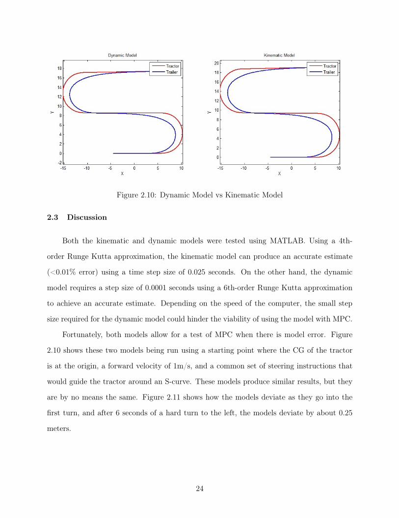
Figure 2.10: Dynamic Model vs Kinematic Model
2.3 Discussion
Both the kinematic and dynamic models were tested using MATLAB. Using a 4th-
order Runge Kutta approximation, the kinematic model can produce an accurate estimate
(<0.01% error) using a time step size of 0.025 seconds. On the other hand, the dynamic
model requires a step size of 0.0001 seconds using a 6th-order Runge Kutta approximation
to achieve an accurate estimate. Depending on the speed of the computer, the small step
size required for the dynamic model could hinder the viability of using the model with MPC.
Fortunately, both models allow for a test of MPC when there is model error. Figure
2.10 shows these two models being run using a starting point where the CG of the tractor
is at the origin, a forward velocity of 1m/s, and a common set of steering instructions that
would guide the tractor around an S-curve. These models produce similar results, but they
are by no means the same. Figure 2.11 shows how the models deviate as they go into the
first turn, and after 6 seconds of a hard turn to the left, the models deviate by about 0.25
meters.
24
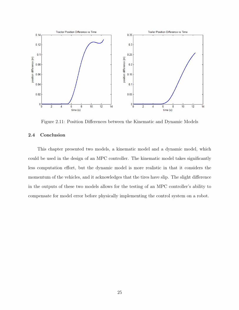
Figure 2.11: Position Differences between the Kinematic and Dynamic Models
2.4 Conclusion
This chapter presented two models, a kinematic model and a dynamic model, which
could be used in the design of an MPC controller. The kinematic model takes significantly
less computation effort, but the dynamic model is more realistic in that it considers the
momentum of the vehicles, and it acknowledges that the tires have slip. The slight difference
in the outputs of these two models allows for the testing of an MPC controller’s ability to
compensate for model error before physically implementing the control system on a robot.
25
Chapter 3
Applying MPC to a Tractor Trailer System
This chapter describes the Model Predictive Control (MPC) algorithm used to control
the tractor-trailer system. First, a front-wheel steering tractor model is considered, followed
by a skid-steering vehicle. MPC follows two key steps: set point calculations, and control
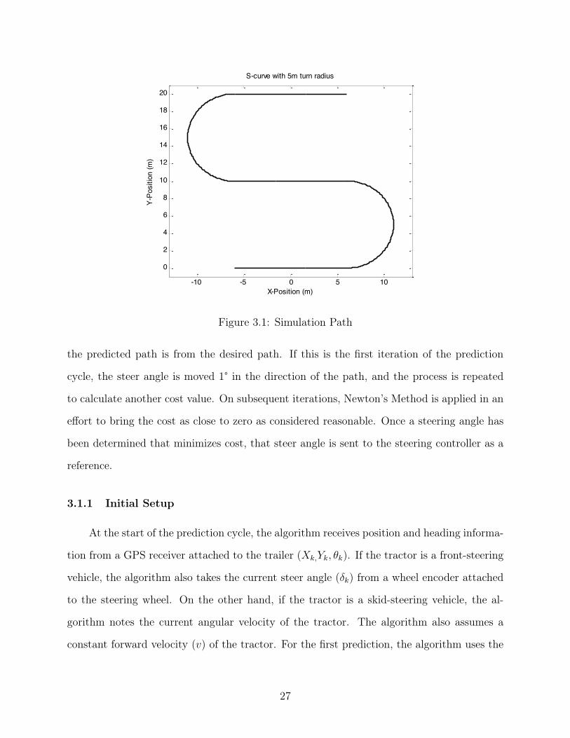
calculations. To test these control methods, an S-curve path was designed with two 5-meter
radius turnarounds as shown in Figure 3.1.
3.1 Set Point Calculations
When learning to drive a motor vehicle, a human driver gradually gains some idea of
how the vehicle will respond to a certain steering input. When preparing to make a turn at
a traffic light (particularly left turns), the driving instructor tells the new driver to visualize
an arc from the vehicle’s current position to where the vehicle will be after making the turn.
When the light turns green, the driver follows the arc, anticipating the car’s response to a
steering input by using preexisting knowledge of the vehicle’s response from previous turns.
In the MPC algorithm, the same principle is applied using a model to predict the outcome,
given a steering input.
Figure 3.2 on page 28 illustrates the steps taken for the set point calculations. Subscript
k indexes how many cycles the set-point calculator has run, while subscript i tracks the
number of guesses the computer has made during its current prediction cycle. Every time
the algorithm recycles, the current position and heading of both the tractor and trailer are
accounted for, and an initial guess is made by using the previous tractor steer angle. The
algorithm then uses the model to predict the path the trailer would follow over next 4 seconds.
Next, using the desired path as a reference, a cost function is calculated based on how far
26
-10 -5 0 5 10
0
2
4
6
8
10
12
14
16
18
20
X-Position (m)
Y-Po
sitio
n (m
)
S-curve with 5m turn radius
Figure 3.1: Simulation Path
the predicted path is from the desired path. If this is the first iteration of the prediction
cycle, the steer angle is moved 1° in the direction of the path, and the process is repeated
to calculate another cost value. On subsequent iterations, Newton’s Method is applied in an
effort to bring the cost as close to zero as considered reasonable. Once a steering angle has
been determined that minimizes cost, that steer angle is sent to the steering controller as a
reference.
3.1.1 Initial Setup
At the start of the prediction cycle, the algorithm receives position and heading informa-
tion from a GPS receiver attached to the trailer (Xk,
Yk
, ✓k
). If the tractor is a front-steering
vehicle, the algorithm also takes the current steer angle (�k
) from a wheel encoder attached
to the steering wheel. On the other hand, if the tractor is a skid-steering vehicle, the al-
gorithm notes the current angular velocity of the tractor. The algorithm also assumes a
constant forward velocity (v) of the tractor. For the first prediction, the algorithm uses the
27
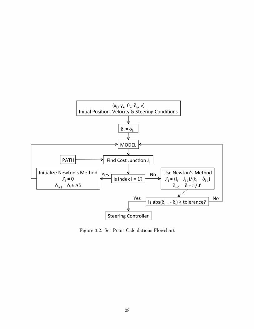
Figure 3.2: Set Point Calculations Flowchart
28
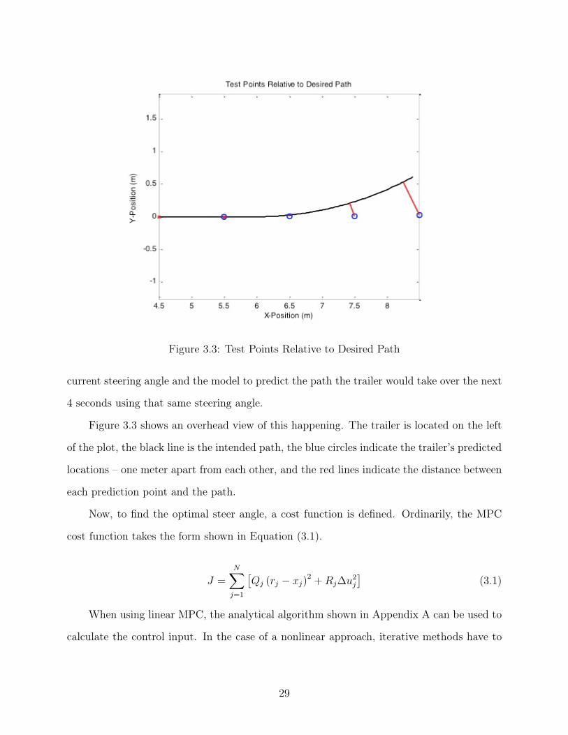
Figure 3.3: Test Points Relative to Desired Path
current steering angle and the model to predict the path the trailer would take over the next
4 seconds using that same steering angle.
Figure 3.3 shows an overhead view of this happening. The trailer is located on the left
of the plot, the black line is the intended path, the blue circles indicate the trailer’s predicted
locations – one meter apart from each other, and the red lines indicate the distance between
each prediction point and the path.
Now, to find the optimal steer angle, a cost function is defined. Ordinarily, the MPC
cost function takes the form shown in Equation (3.1).
J =
NX
j=1
⇥Q
j
(rj
� xj
)
2
+Rj
�u2
j
⇤(3.1)
When using linear MPC, the analytical algorithm shown in Appendix A can be used to
calculate the control input. In the case of a nonlinear approach, iterative methods have to
29
be applied. In many cases, nonlinear MPC is infeasible to implement in real time, but this
research explores a way to reach an input decision quickly.
The cost function is first redefined as the sum of the distances between predicted position
estimates and the path:
Ji
=
�����
4X
j=1
lj
(±1)j
����� (3.2)
where lj
is the shortest distance between the j-th prediction point and the path. To
ensure that this summation converges to zero, all test points to the right of the path are
assigned a positive value, while the test points to the left are assigned a negative value.
Notice that the cost function defined by Equation (3.2) is no longer quadratic, and
instead it has been surrounded by absolute value brackets. Without the absolute value
brackets, the summation could go negative if all prediction points were on the left side of the
path, and a negative cost would imply the existence of a steer input better than optimal.
The absolute value brackets simply state that the length summations that go negative are
just as unfavorable as positive summations.
To determine what the sign should be for each point, some trigonometry is used. First,
the algorithm determines for each point, what angle the path makes with the trailer’s heading
and the nearest point on the path: ✓pathj = arctan
⇣Ypathj
�Ytrailerk
Xpathj�Xtrailerk
⌘. The algorithm then
determines the angle that the prediction point makes with the trailer’s current heading:
✓predj = arctan
⇣Ytrailerj
�Ytrailerk
Xtrailerj�Xtrailerk
⌘. After that, it compares these two angles, and it assigns a
cost function value: Ji
=
���P
4
j=1
lj
· sign�✓pathj � ✓
predj
����.
It is fair to ask a few questions at this point, starting with “Why go to all this effort?”
The reason is that this ensures (in most cases) that the interior of the cost function crosses
zero on the y-axis of a cost versus steer angle plot. This sets things up nicely for using
Newton’s Method to find the zero of the cost function quickly and efficiently. It is important
to point out that this cost function will not return the same solution as Equation (3.1), but
30
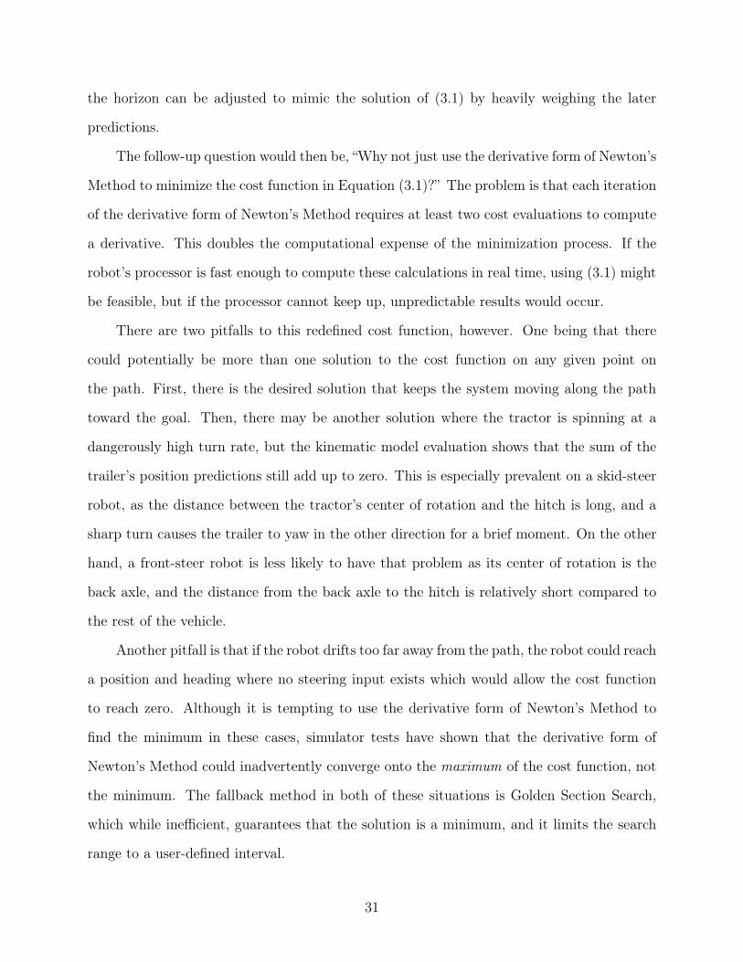
the horizon can be adjusted to mimic the solution of (3.1) by heavily weighing the later
predictions.
The follow-up question would then be, “Why not just use the derivative form of Newton’s
Method to minimize the cost function in Equation (3.1)?” The problem is that each iteration
of the derivative form of Newton’s Method requires at least two cost evaluations to compute
a derivative. This doubles the computational expense of the minimization process. If the
robot’s processor is fast enough to compute these calculations in real time, using (3.1) might
be feasible, but if the processor cannot keep up, unpredictable results would occur.
There are two pitfalls to this redefined cost function, however. One being that there
could potentially be more than one solution to the cost function on any given point on
the path. First, there is the desired solution that keeps the system moving along the path
toward the goal. Then, there may be another solution where the tractor is spinning at a
dangerously high turn rate, but the kinematic model evaluation shows that the sum of the
trailer’s position predictions still add up to zero. This is especially prevalent on a skid-steer
robot, as the distance between the tractor’s center of rotation and the hitch is long, and a
sharp turn causes the trailer to yaw in the other direction for a brief moment. On the other
hand, a front-steer robot is less likely to have that problem as its center of rotation is the
back axle, and the distance from the back axle to the hitch is relatively short compared to
the rest of the vehicle.
Another pitfall is that if the robot drifts too far away from the path, the robot could reach
a position and heading where no steering input exists which would allow the cost function
to reach zero. Although it is tempting to use the derivative form of Newton’s Method to
find the minimum in these cases, simulator tests have shown that the derivative form of
Newton’s Method could inadvertently converge onto the maximum of the cost function, not
the minimum. The fallback method in both of these situations is Golden Section Search,
which while inefficient, guarantees that the solution is a minimum, and it limits the search
range to a user-defined interval.
31
3.1.2 Finding Minimum Cost Using Newton’s Method
Finding the minimum cost is a trial-and-error process, but a good initial guess is the
same steer angle used for the previous prediction cycle. The algorithm uses this guess along
with the model to predict where the tractor and trailer would go. Then, the second guess is
1° to the right or left of that angle (depending on which side of the initial guess the path is
on). With two points available, the algorithm can now predict a third point using Equations
(3.3) and (3.4).
J 0i
=
Ji
� Ji�1
�i
� �i�1
(3.3)
�i+1
= �i
� Ji
J 0i
(3.4)
Figure 3.4 on page 33 illustrates the Newton’s Method process. Each frame in Figure
3.4 depicts the results of a prediction. On the top subplot of each frame, the trailer GPS
receiver is located on the far left-hand side of the plot. The black line is the path. The blue
circles are prediction points based off of the model, one second apart from each other. The
red lines represent the distance from each point to the path. On the bottom subplot of each
frame, the x-axis is the steering angle, while the y-axis is the cost. The blue line is the cost
function that occurs under the current tractor-trailer state conditions, which was computed
only for this demonstration, but is impractical to compute in real time. Finally, the red line
tracks each prediction made using Newton’s Method.
The cycle repeats itself until the change in steer angle is less than 0.5°. As seen in
the Figure, the prediction algorithm ran five times to arrive at the steering angle with a
cost near zero. By reusing the previously calculated steering angle, however, the algorithm
usually arrives at a usable steering angle after three predictions. Figure 3.5 on page 34
shows an overhead simulation of the system guiding to the path using this MPC approach,
assuming the controller could guide to the set points instantaneously.
32
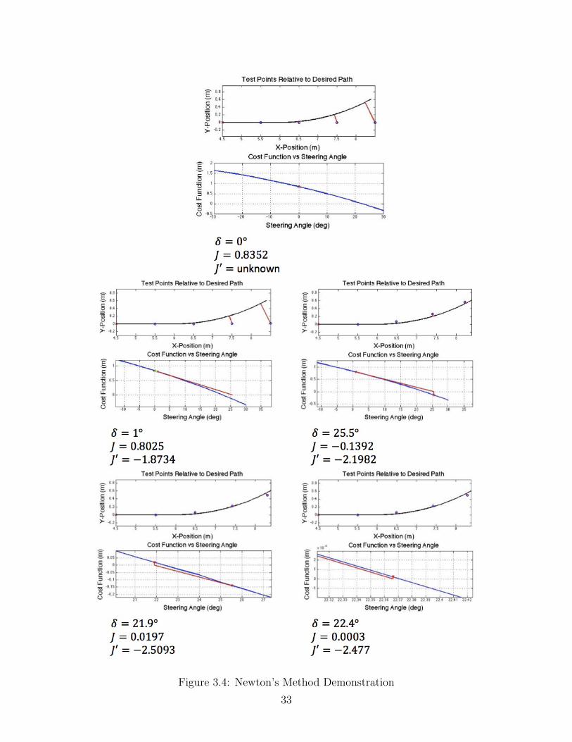
Figure 3.4: Newton’s Method Demonstration33
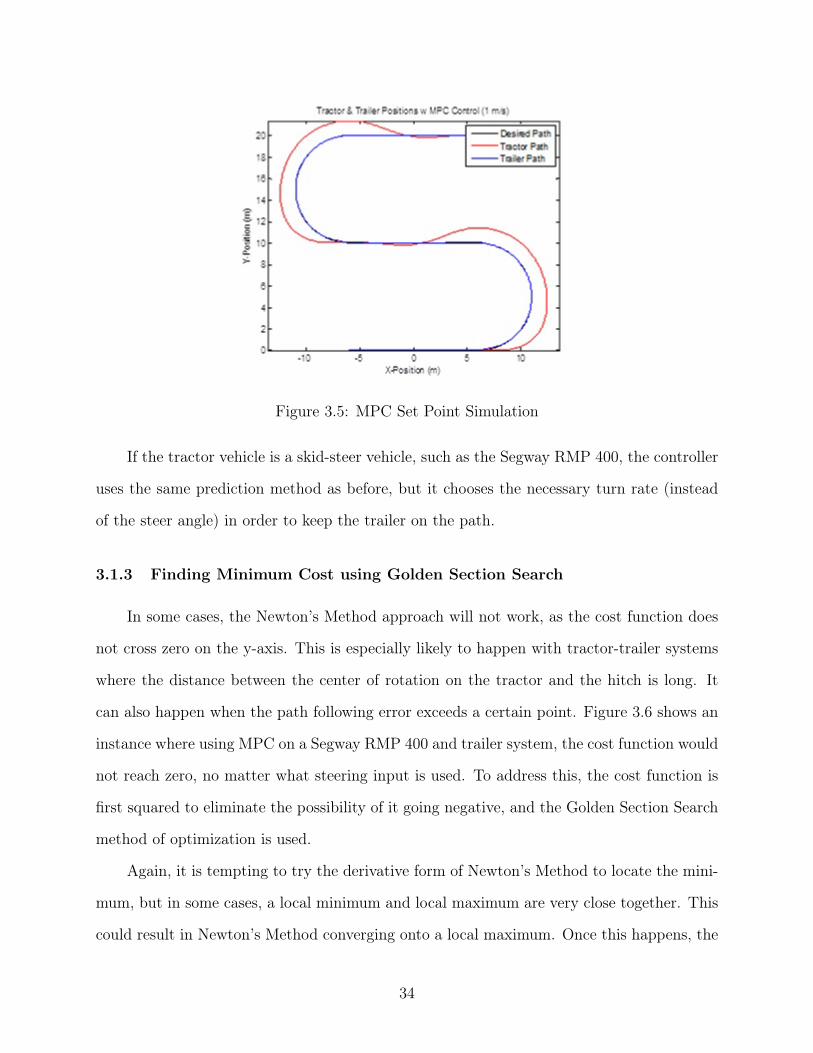
Figure 3.5: MPC Set Point Simulation
If the tractor vehicle is a skid-steer vehicle, such as the Segway RMP 400, the controller
uses the same prediction method as before, but it chooses the necessary turn rate (instead
of the steer angle) in order to keep the trailer on the path.
3.1.3 Finding Minimum Cost using Golden Section Search
In some cases, the Newton’s Method approach will not work, as the cost function does
not cross zero on the y-axis. This is especially likely to happen with tractor-trailer systems
where the distance between the center of rotation on the tractor and the hitch is long. It
can also happen when the path following error exceeds a certain point. Figure 3.6 shows an
instance where using MPC on a Segway RMP 400 and trailer system, the cost function would
not reach zero, no matter what steering input is used. To address this, the cost function is
first squared to eliminate the possibility of it going negative, and the Golden Section Search
method of optimization is used.
Again, it is tempting to try the derivative form of Newton’s Method to locate the mini-
mum, but in some cases, a local minimum and local maximum are very close together. This
could result in Newton’s Method converging onto a local maximum. Once this happens, the
34

Figure 3.6: Newton’s Method Incompatibility
robot continues to follow this method, maintaining its steering input on the local maximum
of the cost function and loses the path completely. On the other hand, the Golden Section
Search method guarantees a minimum, provided that a local minimum exists on the chosen
interval.[16]
The prediction points for the Golden Section search method are chosen the following
way. First a prediction interval is chosen (in the case of the Segway, -40 deg/sec to 40
deg/sec). If l0
defines the length of the full interval, and l1
and l2
define the space between
the left and right edges of the interval and the intermediate prediction points, the locations
of l1
and l2
can be determined by satisfying the following conditions:
l1
+ l2
= l0
(3.5)
l1
l0
=
l2
l1
(3.6)
By substituting Equation (3.5) into Equation (3.6), the following equation results:
35
l1
l1
+ l2
=
l2
l1
(3.7)
Next, the reciprocal is taken, and R is defined as l
2
l
1
, resulting in the following:
1 +R =
1
R(3.8)
By multiplying both sides by R, Equation (3.8) becomes R2
+R�1 = 0, and the positive
root, or the golden ratio can be solved for. The result is R =
p5�1
2
t 0.61803.
To set up the algorithm, xl
and xu
define steer inputs at the lower and upper limits of
the prediction interval. The intermediate points x1
and x2
are then chosen using the golden
ratio:
x1
= xl
+
p5� 1
2
(xu
� xl
) (3.9)
x2
= xu
�p5� 1
2
(xu
� xl
) (3.10)
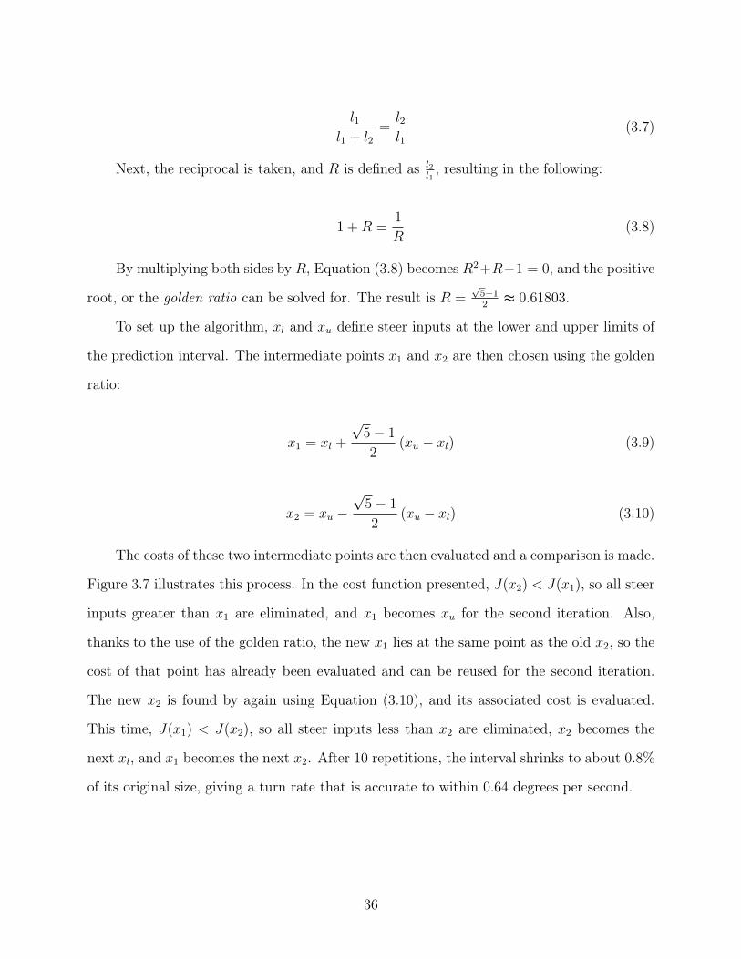
The costs of these two intermediate points are then evaluated and a comparison is made.
Figure 3.7 illustrates this process. In the cost function presented, J(x2
) < J(x1
), so all steer
inputs greater than x1
are eliminated, and x1
becomes xu
for the second iteration. Also,
thanks to the use of the golden ratio, the new x1
lies at the same point as the old x2
, so the
cost of that point has already been evaluated and can be reused for the second iteration.
The new x2
is found by again using Equation (3.10), and its associated cost is evaluated.
This time, J(x1
) < J(x2
), so all steer inputs less than x2
are eliminated, x2
becomes the
next xl
, and x1
becomes the next x2
. After 10 repetitions, the interval shrinks to about 0.8%
of its original size, giving a turn rate that is accurate to within 0.64 degrees per second.
36
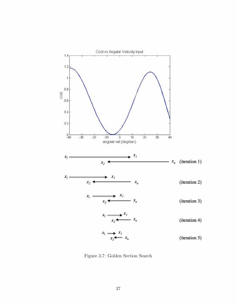
Figure 3.7: Golden Section Search
37
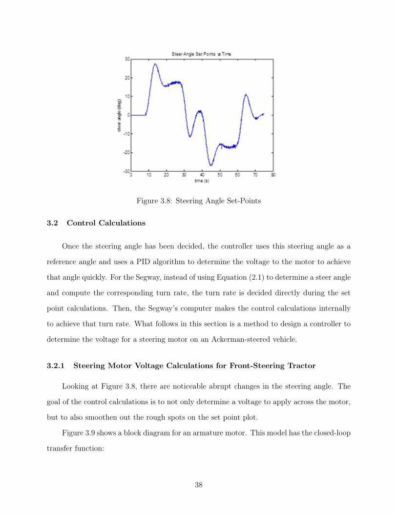
Figure 3.8: Steering Angle Set-Points
3.2 Control Calculations
Once the steering angle has been decided, the controller uses this steering angle as a
reference angle and uses a PID algorithm to determine the voltage to the motor to achieve
that angle quickly. For the Segway, instead of using Equation (2.1) to determine a steer angle
and compute the corresponding turn rate, the turn rate is decided directly during the set
point calculations. Then, the Segway’s computer makes the control calculations internally
to achieve that turn rate. What follows in this section is a method to design a controller to
determine the voltage for a steering motor on an Ackerman-steered vehicle.
3.2.1 Steering Motor Voltage Calculations for Front-Steering Tractor
Looking at Figure 3.8, there are noticeable abrupt changes in the steering angle. The
goal of the control calculations is to not only determine a voltage to apply across the motor,
but to also smoothen out the rough spots on the set point plot.
Figure 3.9 shows a block diagram for an armature motor. This model has the closed-loop
transfer function:
38
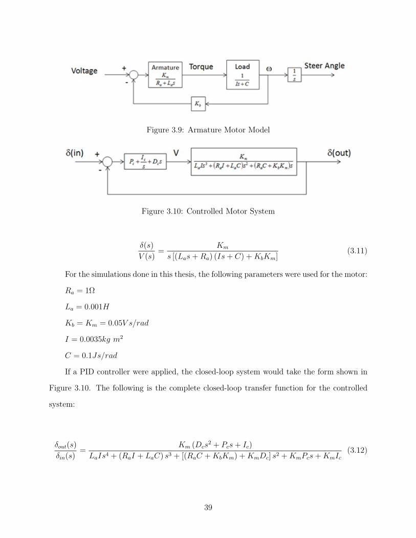
Figure 3.9: Armature Motor Model
Figure 3.10: Controlled Motor System
�(s)
V (s)=
Km
s [(La
s+Ra
) (Is+ C) +Kb
Km
]
(3.11)
For the simulations done in this thesis, the following parameters were used for the motor:
Ra
= 1⌦
La
= 0.001H
Kb
= Km
= 0.05V s/rad
I = 0.0035kg m2
C = 0.1Js/rad
If a PID controller were applied, the closed-loop system would take the form shown in
Figure 3.10. The following is the complete closed-loop transfer function for the controlled
system:
�out
(s)
�in
(s)=
Km
(Dc
s2 + Pc
s+ Ic
)
La
Is4 + (Ra
I + La
C) s3 + [(Ra
C +Kb
Km
) +Km
Dc
] s2 +Km
Pc
s+Km
Ic
(3.12)
39
23 23.1 23.2 23.3 23.4 23.5 23.6 23.7 23.8 23.9 2415.5
16
16.5
17
17.5
18
18.5
time (s)
stee
r ang
le (d
eg)
Steer Angle Set Points vs Time
Figure 3.11: Unwanted Oscillations
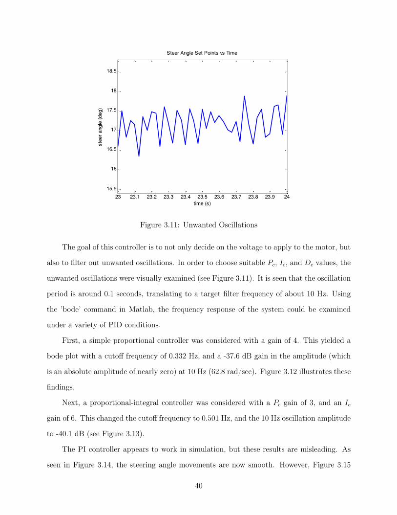
The goal of this controller is to not only decide on the voltage to apply to the motor, but
also to filter out unwanted oscillations. In order to choose suitable Pc
, Ic
, and Dc
values, the
unwanted oscillations were visually examined (see Figure 3.11). It is seen that the oscillation
period is around 0.1 seconds, translating to a target filter frequency of about 10 Hz. Using
the ’bode’ command in Matlab, the frequency response of the system could be examined
under a variety of PID conditions.
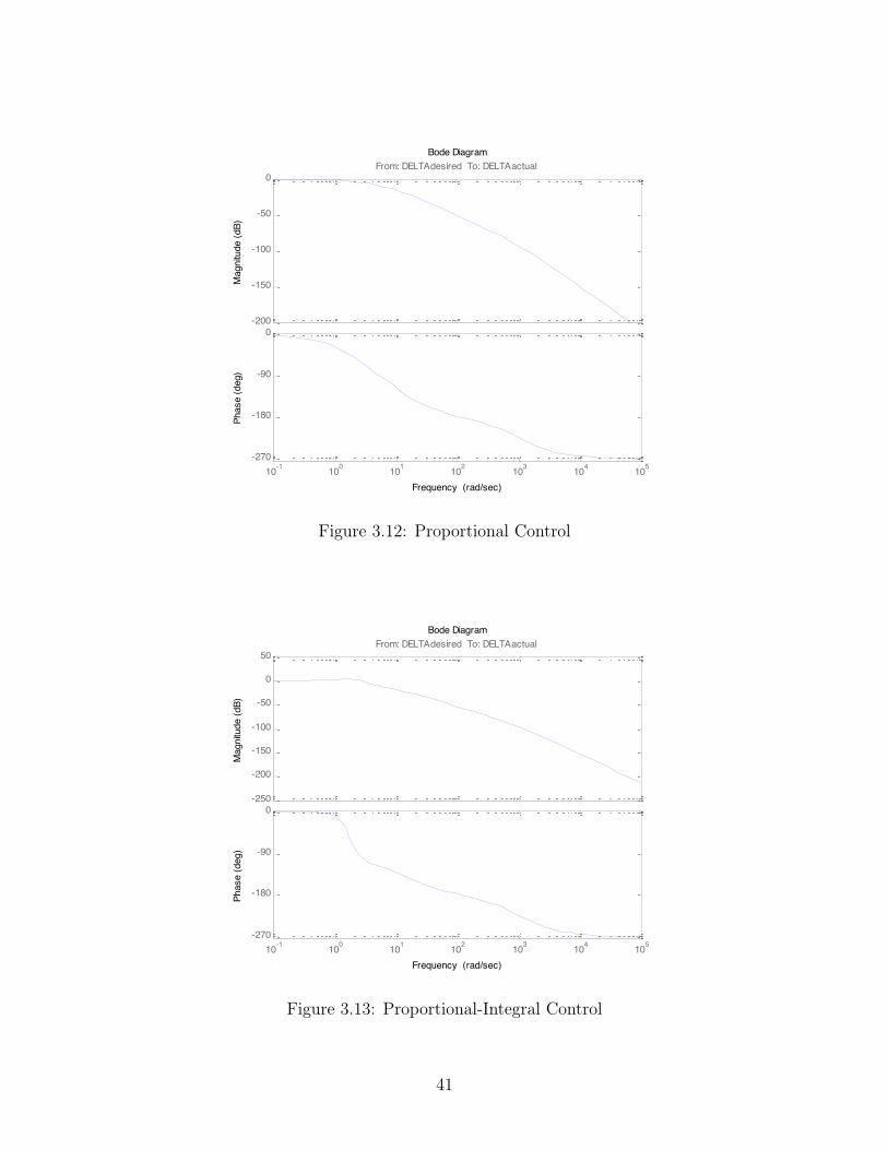
First, a simple proportional controller was considered with a gain of 4. This yielded a
bode plot with a cutoff frequency of 0.332 Hz, and a -37.6 dB gain in the amplitude (which
is an absolute amplitude of nearly zero) at 10 Hz (62.8 rad/sec). Figure 3.12 illustrates these
findings.
Next, a proportional-integral controller was considered with a Pc
gain of 3, and an Ic
gain of 6. This changed the cutoff frequency to 0.501 Hz, and the 10 Hz oscillation amplitude
to -40.1 dB (see Figure 3.13).
The PI controller appears to work in simulation, but these results are misleading. As
seen in Figure 3.14, the steering angle movements are now smooth. However, Figure 3.15
40
-200
-150
-100
-50
0From: DELTAdesired To: DELTAactual
Mag
nitu
de (d
B)
10-1 100 101 102 103 104 105-270
-180
-90
0
Phas
e (d
eg)
Bode Diagram
Frequency (rad/sec)
Figure 3.12: Proportional Control
-250
-200
-150
-100
-50
0
50From: DELTAdesired To: DELTAactual
Mag
nitu
de (d
B)
10-1 100 101 102 103 104 105-270
-180
-90
0
Phas
e (d
eg)
Bode Diagram
Frequency (rad/sec)
Figure 3.13: Proportional-Integral Control
41

0 10 20 30 40 50 60 70 80-30
-20
-10
0
10
20
30
time (s)
stee
r ang
le (d
eg)
Steer Angle vs Time
Figure 3.14: Steer Angle Controlled
Figure 3.15: Voltage Across Motor vs Time (using PI control)
42
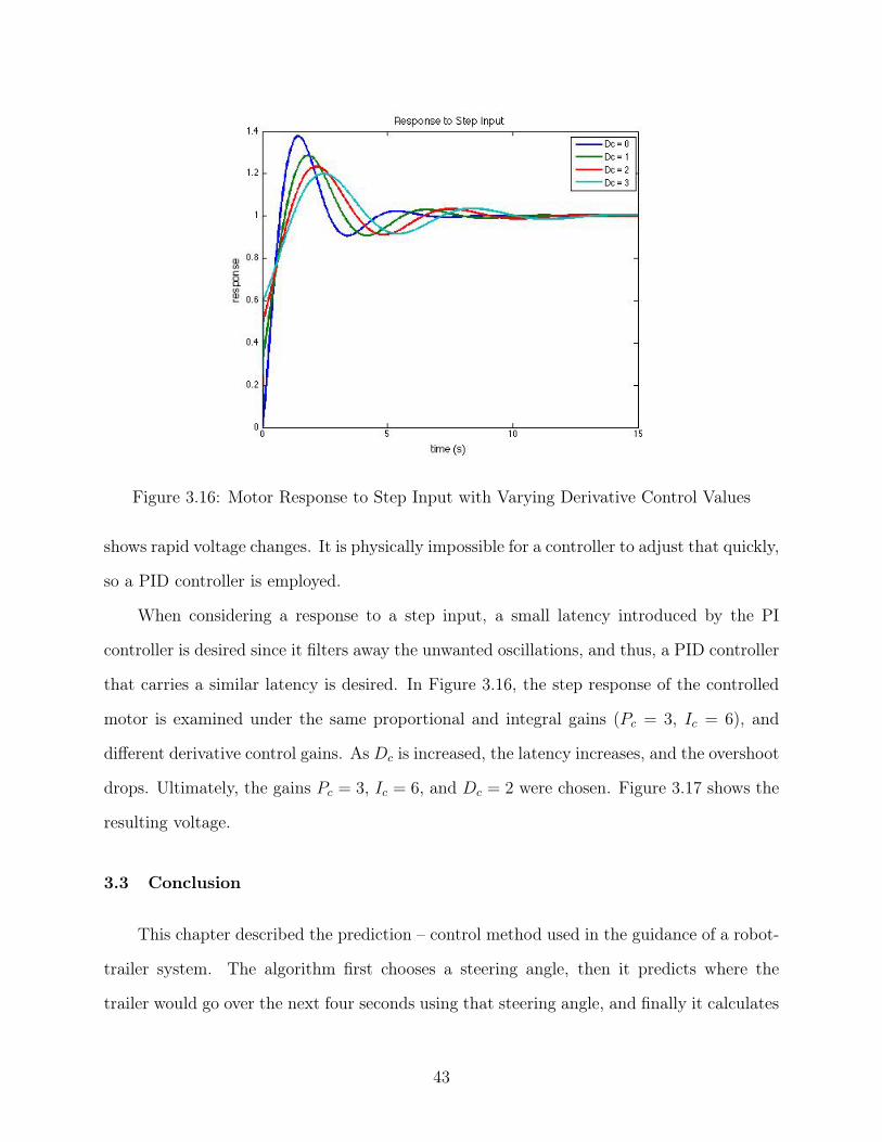
Figure 3.16: Motor Response to Step Input with Varying Derivative Control Values
shows rapid voltage changes. It is physically impossible for a controller to adjust that quickly,
so a PID controller is employed.
When considering a response to a step input, a small latency introduced by the PI
controller is desired since it filters away the unwanted oscillations, and thus, a PID controller
that carries a similar latency is desired. In Figure 3.16, the step response of the controlled
motor is examined under the same proportional and integral gains (Pc
= 3, Ic
= 6), and
different derivative control gains. As Dc
is increased, the latency increases, and the overshoot
drops. Ultimately, the gains Pc
= 3, Ic
= 6, and Dc
= 2 were chosen. Figure 3.17 shows the
resulting voltage.
3.3 Conclusion
This chapter described the prediction – control method used in the guidance of a robot-
trailer system. The algorithm first chooses a steering angle, then it predicts where the
trailer would go over the next four seconds using that steering angle, and finally it calculates
43
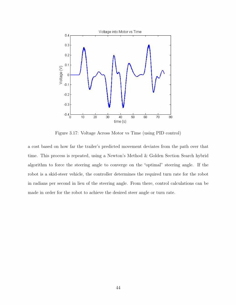
Figure 3.17: Voltage Across Motor vs Time (using PID control)
a cost based on how far the trailer’s predicted movement deviates from the path over that
time. This process is repeated, using a Newton’s Method & Golden Section Search hybrid
algorithm to force the steering angle to converge on the “optimal” steering angle. If the
robot is a skid-steer vehicle, the controller determines the required turn rate for the robot
in radians per second in lieu of the steering angle. From there, control calculations can be
made in order for the robot to achieve the desired steer angle or turn rate.
44
Chapter 4
Computer Simulations and Live Application
This chapter presents the observations made by running various computer simulations,
as well as a live application, using this controller. First, since this control system was
originally intended to be used on an Ackerman-steered vehicle, the controller’s performance
was examined against a bicycle model under varying turn radii. Next, a simulation was
done using a real-time simulator for a differential-steered robot. Finally, this controller was
uploaded onto a Segway RMP 400 robot and examined.
4.1 Kubota RTV Simulation Results
Although the hardware for the Kubota RTV is still being assembled at the time of
this thesis writing, it is still possible to simulate how the controller will behave when the
plant’s response to an input does not match the model’s prediction exactly. For the first
simulation, the MPC simulator is modified to use the kinematic model to generate predictions
and determine inputs, and then use the dynamic bicycle model to simulate the Kubota’s
response. For the second simulation, the MPC simulator uses the linearized kinematic model
to generate predictions, and then it uses the nonlinear kinematic model to simulate Kubota’s
response.
4.1.1 Kinematic Controller Model against Bicycle Plant Model
As expected, when the controller model does not match reality, the controller is subject
to significant error. Figure 4.1 shows an overhead view of the tractor-trailer path following
under these conditions, while Figure 4.2 shows the error. The straight, middle section of the
S-curve is between 30 and 42 seconds on the time plots.
45

Figure 4.1: MPC with Model Error
Figure 4.2: Deviation with High Model Error
46

Figure 4.3: Deviation with Low Model Error
Several attempts were made to tune the controller in order to compensate for the model
error. First, the prediction horizon length was varied to three seconds, five seconds, and six
seconds. None of these changes reduced the maximum error. Longer prediction horizons
resulted in more gradual corrections, while shorter prediction horizons caused more abrupt
corrections. A prediction horizon of 4 seconds produced the least amount of error on the
path turns. Second, weights were added to each prediction point (i.e. the prediction point
one second ahead was multiplied by a factor of 4, the second by 3, the third by 2, and the
fourth by 1). The results were similar to shortening the prediction horizon, where the tractor
would turn more violently to compensate for error. In fact, weighing the earlier points by
too high a factor (or having too short of a prediction horizon) would cause the tractor to
veer off the path to the point of losing the path entirely and starts driving around in circles.
Conversely, a simulation was run with the kinematic model serving as the plant model
as well as the prediction model. This would simulate what would happen if the model closely
reflects the actual plant. Figure 4.3 shows the deviation from the path with a highly accurate
47

Figure 4.4: Wide S-curve Path Following
model. As seen with this model, the controller is still subject to error. The next section
examines this more closely.
4.1.2 Linearized Kinematic Controller Model against Nonlinear Kinematic Plant
Model
For the second simulation, the S-curve was widened so that the straight sections would
be 30 meters long. This would allow for better observation of the settling time of the path
following.
Figures 4.5 and 4.6 show the path following using the nonlinear and linear control
models, respectively. Both models do well when following the straight sections of the path,
but the nonlinear model appears to track toward the path even in the turns. In addition,
since both models choose their turn rates based on future predictions, they have a tendency to
make their steering adjustments early. This leads to the largest error being at the beginning
and end of each turn.
48

Figure 4.5: Path Following Using Nonlinear Control Model
Figure 4.6: Path Following Using Linear Control Model
49

Figure 4.7: 15m Radius S-curve
Figure 4.8: Path Following Using Nonlinear Control Model (15m radius)
50

Figure 4.9: Path Following Using Linear Control Model (15m radius)
To further study this, another S-curve was made with a 15 meter turn radius. Now,
steady-state error could be studied on the turns. By comparing the nonlinear controller
(Figure 4.8) to the linear controller (Figure 4.9), it is seen that the nonlinear controller has
a steady-state error much closer to zero than the linear controller on the turns. As seen in
this simulation study, the steady-state error with the linear controller increases as the turn
radius decreases, but with large turn radii, nonlinear control becomes unnecessary.
4.2 Segway Simulation Results
Next, in preparation for a live run on an autonomous vehicle, the MPC algorithm was
converted from Matlab code to C++. In addition a ROS (Robot Operating System) node
was written into the C++ code in order to communicate the intended control inputs to the
robot. To verify that the ROS node was working properly, a test was run using the ROS
node against a simulator for the Segway [18]. This simulator introduces a realistic amount
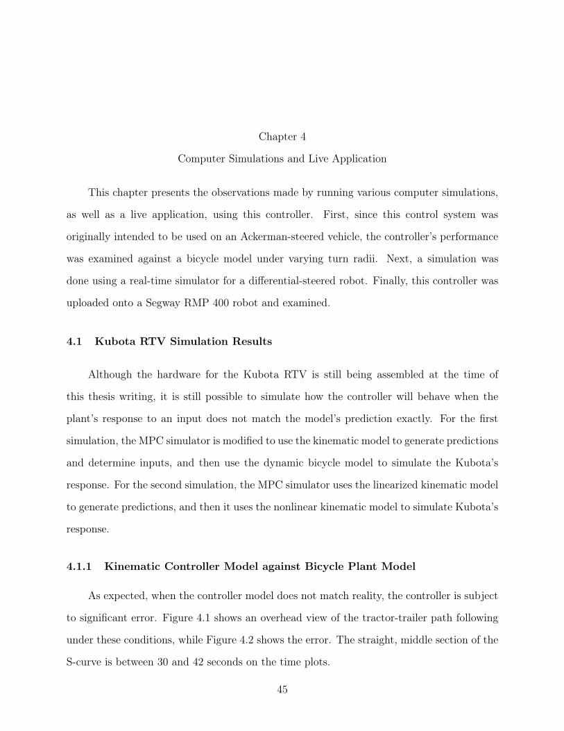
51
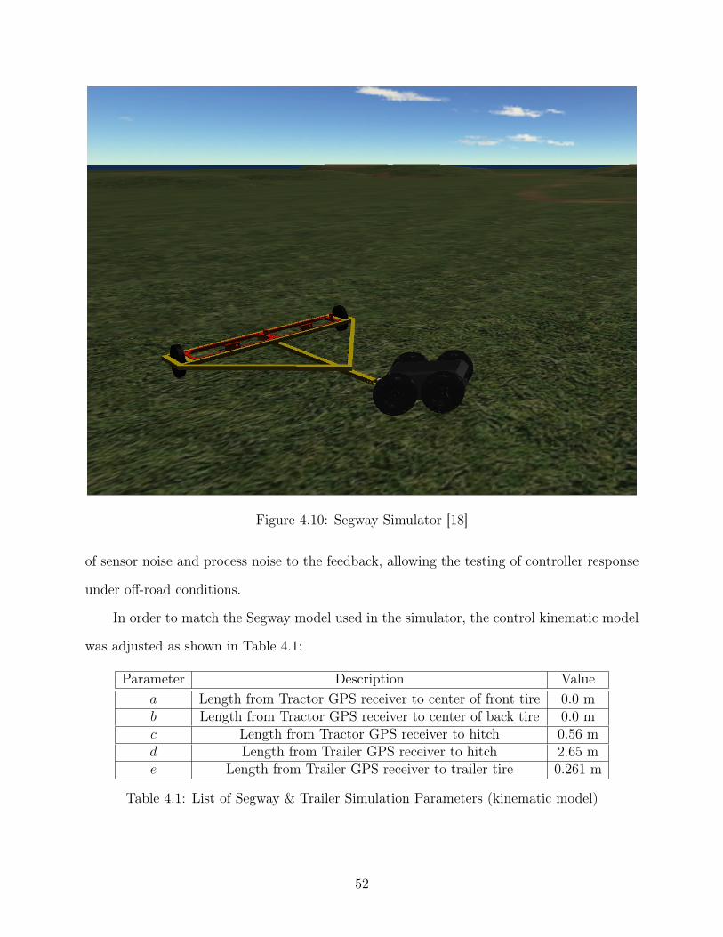
Figure 4.10: Segway Simulator [18]
of sensor noise and process noise to the feedback, allowing the testing of controller response
under off-road conditions.
In order to match the Segway model used in the simulator, the control kinematic model
was adjusted as shown in Table 4.1:
Parameter Description Valuea Length from Tractor GPS receiver to center of front tire 0.0 mb Length from Tractor GPS receiver to center of back tire 0.0 mc Length from Tractor GPS receiver to hitch 0.56 md Length from Trailer GPS receiver to hitch 2.65 me Length from Trailer GPS receiver to trailer tire 0.261 m
Table 4.1: List of Segway & Trailer Simulation Parameters (kinematic model)
52
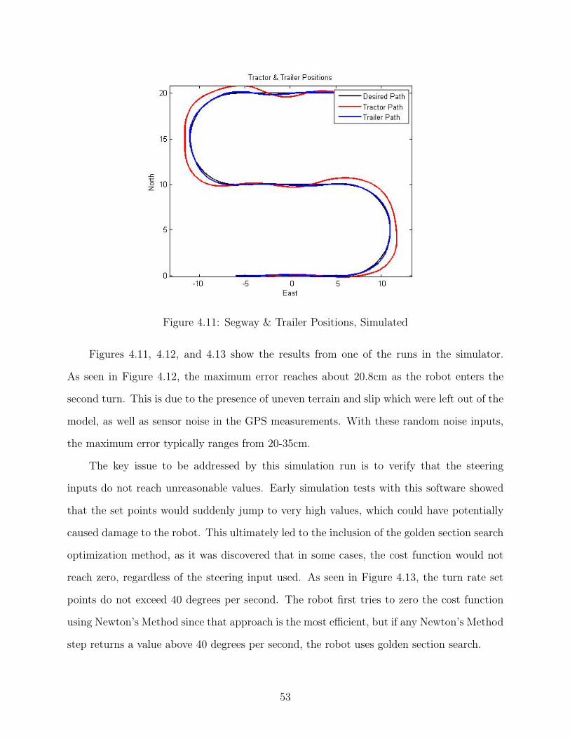
Figure 4.11: Segway & Trailer Positions, Simulated
Figures 4.11, 4.12, and 4.13 show the results from one of the runs in the simulator.
As seen in Figure 4.12, the maximum error reaches about 20.8cm as the robot enters the
second turn. This is due to the presence of uneven terrain and slip which were left out of the
model, as well as sensor noise in the GPS measurements. With these random noise inputs,
the maximum error typically ranges from 20-35cm.
The key issue to be addressed by this simulation run is to verify that the steering
inputs do not reach unreasonable values. Early simulation tests with this software showed
that the set points would suddenly jump to very high values, which could have potentially
caused damage to the robot. This ultimately led to the inclusion of the golden section search
optimization method, as it was discovered that in some cases, the cost function would not
reach zero, regardless of the steering input used. As seen in Figure 4.13, the turn rate set
points do not exceed 40 degrees per second. The robot first tries to zero the cost function
using Newton’s Method since that approach is the most efficient, but if any Newton’s Method
step returns a value above 40 degrees per second, the robot uses golden section search.
53
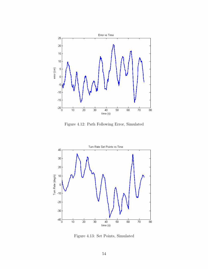
Figure 4.12: Path Following Error, Simulated
Figure 4.13: Set Points, Simulated
54
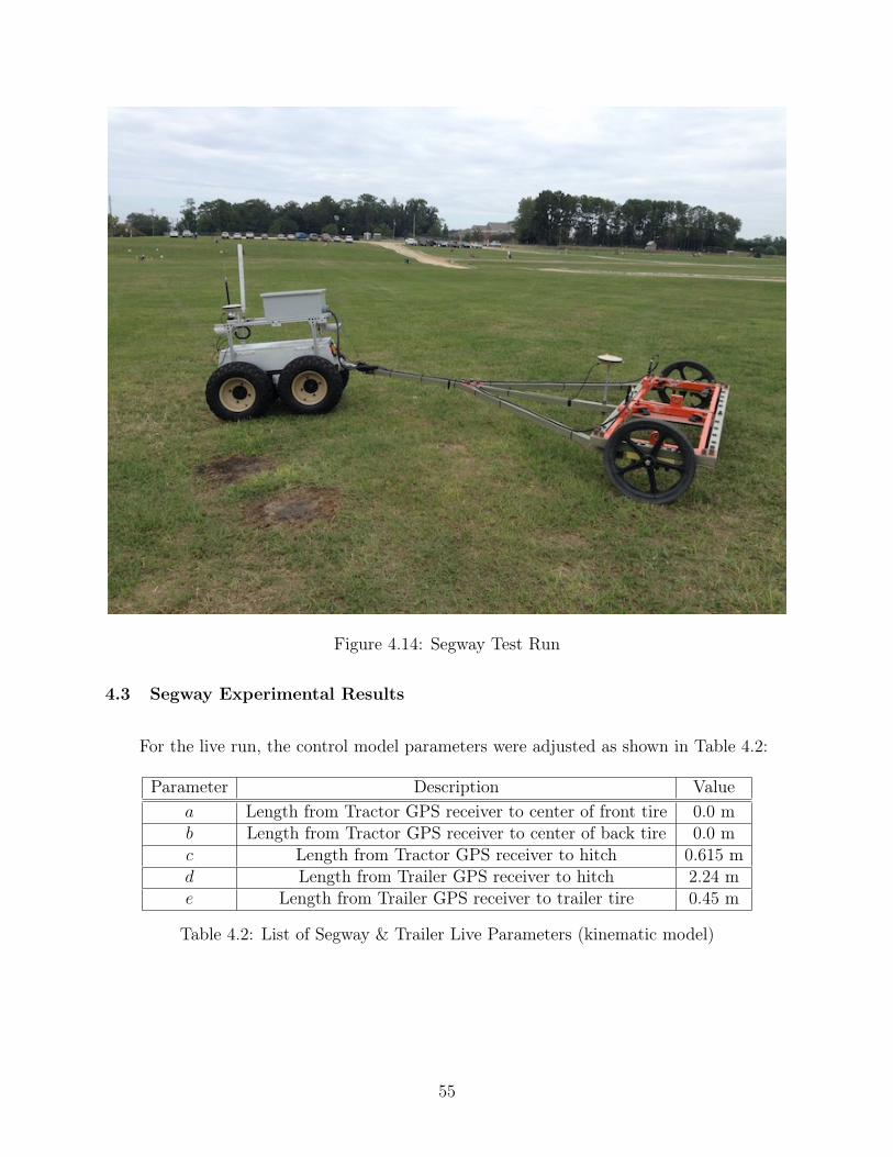
Figure 4.14: Segway Test Run
4.3 Segway Experimental Results
For the live run, the control model parameters were adjusted as shown in Table 4.2:
Parameter Description Valuea Length from Tractor GPS receiver to center of front tire 0.0 mb Length from Tractor GPS receiver to center of back tire 0.0 mc Length from Tractor GPS receiver to hitch 0.615 md Length from Trailer GPS receiver to hitch 2.24 me Length from Trailer GPS receiver to trailer tire 0.45 m
Table 4.2: List of Segway & Trailer Live Parameters (kinematic model)
55
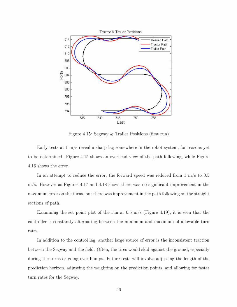
Figure 4.15: Segway & Trailer Positions (first run)
Early tests at 1 m/s reveal a sharp lag somewhere in the robot system, for reasons yet
to be determined. Figure 4.15 shows an overhead view of the path following, while Figure
4.16 shows the error.
In an attempt to reduce the error, the forward speed was reduced from 1 m/s to 0.5
m/s. However as Figures 4.17 and 4.18 show, there was no significant improvement in the
maximum error on the turns, but there was improvement in the path following on the straight
sections of path.
Examining the set point plot of the run at 0.5 m/s (Figure 4.19), it is seen that the
controller is constantly alternating between the minimum and maximum of allowable turn
rates.
In addition to the control lag, another large source of error is the inconsistent traction
between the Segway and the field. Often, the tires would skid against the ground, especially
during the turns or going over bumps. Future tests will involve adjusting the length of the
prediction horizon, adjusting the weighting on the prediction points, and allowing for faster
turn rates for the Segway.
56
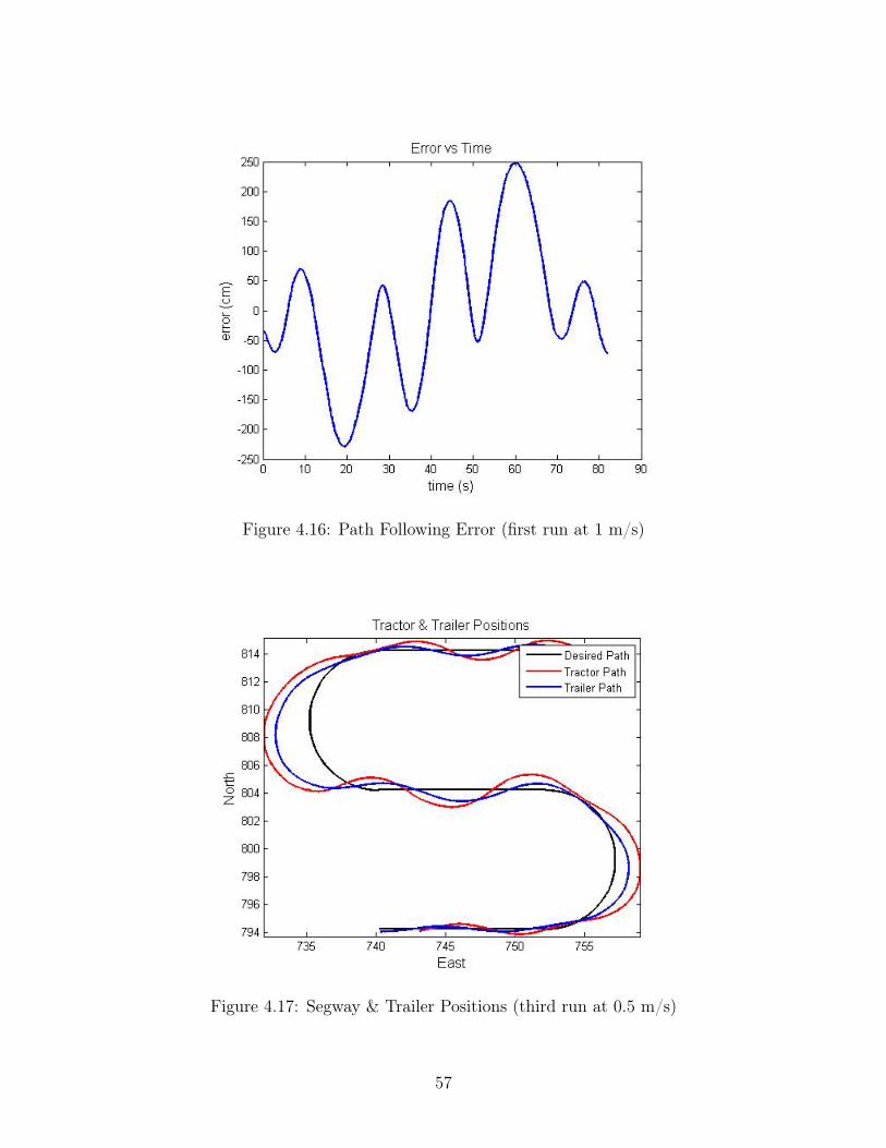
Figure 4.16: Path Following Error (first run at 1 m/s)
Figure 4.17: Segway & Trailer Positions (third run at 0.5 m/s)
57
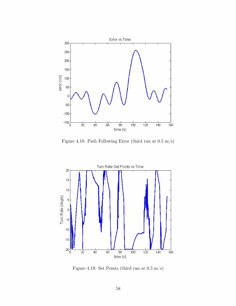
Figure 4.18: Path Following Error (third run at 0.5 m/s)
Figure 4.19: Set Points (third run at 0.5 m/s)
58

Figure 4.20: Results with 4m prediction horizon, weighted
4.3.1 Controller Tuning
To help examine the performance of the controller, the straight sections of the S-curve
were widened from 12 meters to 30 meters. For safety reasons, the speed of the tractor
was limited to 0.5 meters. Initially, a prediction horizon of 4 meters was chosen, and each
prediction point was weighted by scaling them heavier near the trailer, and scaling them
lighter away from the trailer, as shown in Table 4.3:
Distance from Robot Scale Factor1 meter
p4
2 metersp3
3 metersp2
4 metersp1
Table 4.3: Scale Factors
With a 4 meter prediction horizon, weighted using the scale factors of Table 4.3, a
path following performance shown in Figure 4.20 results. While these controller parameters
worked fine in simulation, they produce unstable results on the physical robot.
Next, a 4 meter horizon without weights was tried, as shown in Figure 4.21. The results
suggest that the controller is no longer unstable, but there is no evidence that the controller
would reach steady state.
59
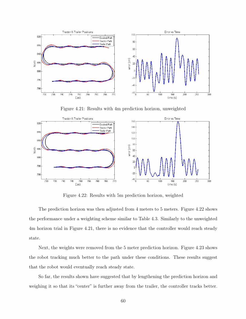
Figure 4.21: Results with 4m prediction horizon, unweighted
Figure 4.22: Results with 5m prediction horizon, weighted
The prediction horizon was then adjusted from 4 meters to 5 meters. Figure 4.22 shows
the performance under a weighting scheme similar to Table 4.3. Similarly to the unweighted
4m horizon trial in Figure 4.21, there is no evidence that the controller would reach steady
state.
Next, the weights were removed from the 5 meter prediction horizon. Figure 4.23 shows
the robot tracking much better to the path under these conditions. These results suggest
that the robot would eventually reach steady state.
So far, the results shown have suggested that by lengthening the prediction horizon and
weighing it so that its “center” is further away from the trailer, the controller tracks better.
60

Figure 4.23: Results with 5m prediction horizon, unweighted
With that in mind, a prediction horizon of 6 meters was tried, but it failed as the computer
speed of the robot was not fast enough to process the calculations in time. To compensate
for this limitation, the 5 meter horizon was kept, but the weighting of the prediction points
was shifted forward by using the scaling factors in Table 4.4:
Distance from Robot Scale Factor1 meter
p1
2 metersp2
3 metersp3
4 metersp4
5 metersp5
Table 4.4: Inverted Scale Factors
Figure 4.24 shows the robot performance with a prediction horizon of 5 meters, using
this inverted weighing scheme. Now, the robot converges onto the path much more quickly,
and the oscillations appear to have a half-life of roughly 25 meters.
Next, the horizon was reduced back to 4 meters, and the same inverted weighting scheme
was used. The results, shown in Figure 4.25, show that the oscillations converge more slowly
than with the 5 meter horizon. It should be noted that when using the 4 meter horizon with
the inverted weighting, as well as when using the unweighted 5 meter horizon, the trailer
tracked the turns better than with the 5 meter horizon with inverted weighting.
61
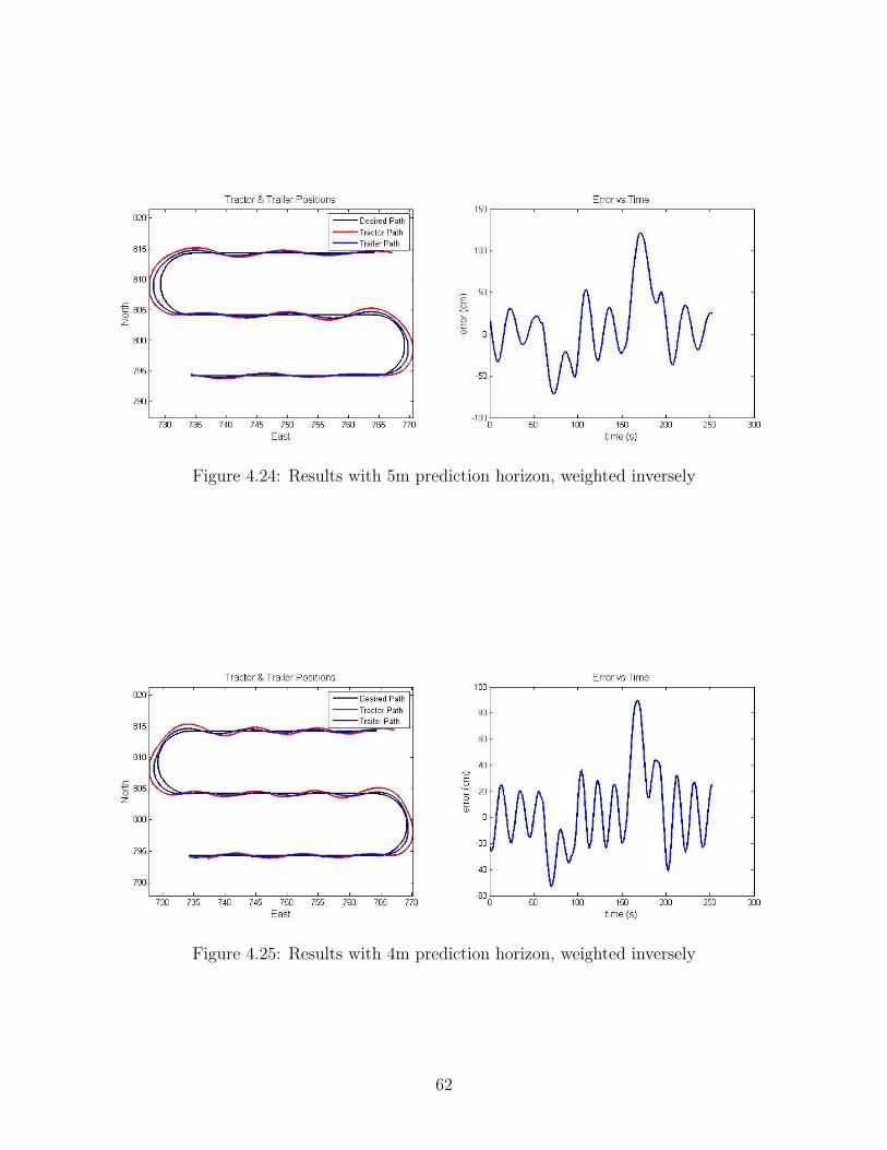
Figure 4.24: Results with 5m prediction horizon, weighted inversely
Figure 4.25: Results with 4m prediction horizon, weighted inversely
62

Figure 4.26: Results with 5m prediction horizon, weighted inversely, one-to-one
Figure 4.27: Results with 4m prediction horizon, weighted inversely, one-to-one
Finally, a one-to-one horizon weighting scheme was chosen, illustrated in Table 4.5:
Distance from Robot Scale Factor1 meter 12 meters 23 meters 34 meters 45 meters 5
Table 4.5: Inverted Scale Factors, One-to-One
Figures 4.26 and 4.27 show the results under the one-to-one weighting scheme. From
these results, it is found that the 4 meter prediction horizon produces the most accurate
63
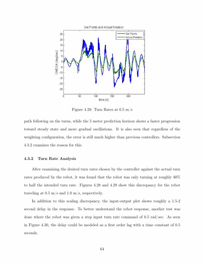
Figure 4.28: Turn Rates at 0.5 m/s
path following on the turns, while the 5 meter prediction horizon shows a faster progression
toward steady state and more gradual oscillations. It is also seen that regardless of the
weighting configuration, the error is still much higher than previous controllers. Subsection
4.3.2 examines the reason for this.
4.3.2 Turn Rate Analysis
After examining the desired turn rates chosen by the controller against the actual turn
rates produced by the robot, it was found that the robot was only turning at roughly 40%
to half the intended turn rate. Figures 4.28 and 4.29 show this discrepancy for the robot
traveling at 0.5 m/s and 1.0 m/s, respectively.
In addition to this scaling discrepancy, the input-output plot shows roughly a 1.5-2
second delay in the response. To better understand the robot response, another test was
done where the robot was given a step input turn rate command of 0.5 rad/sec. As seen
in Figure 4.30, the delay could be modeled as a first order lag with a time constant of 0.5
seconds.
64
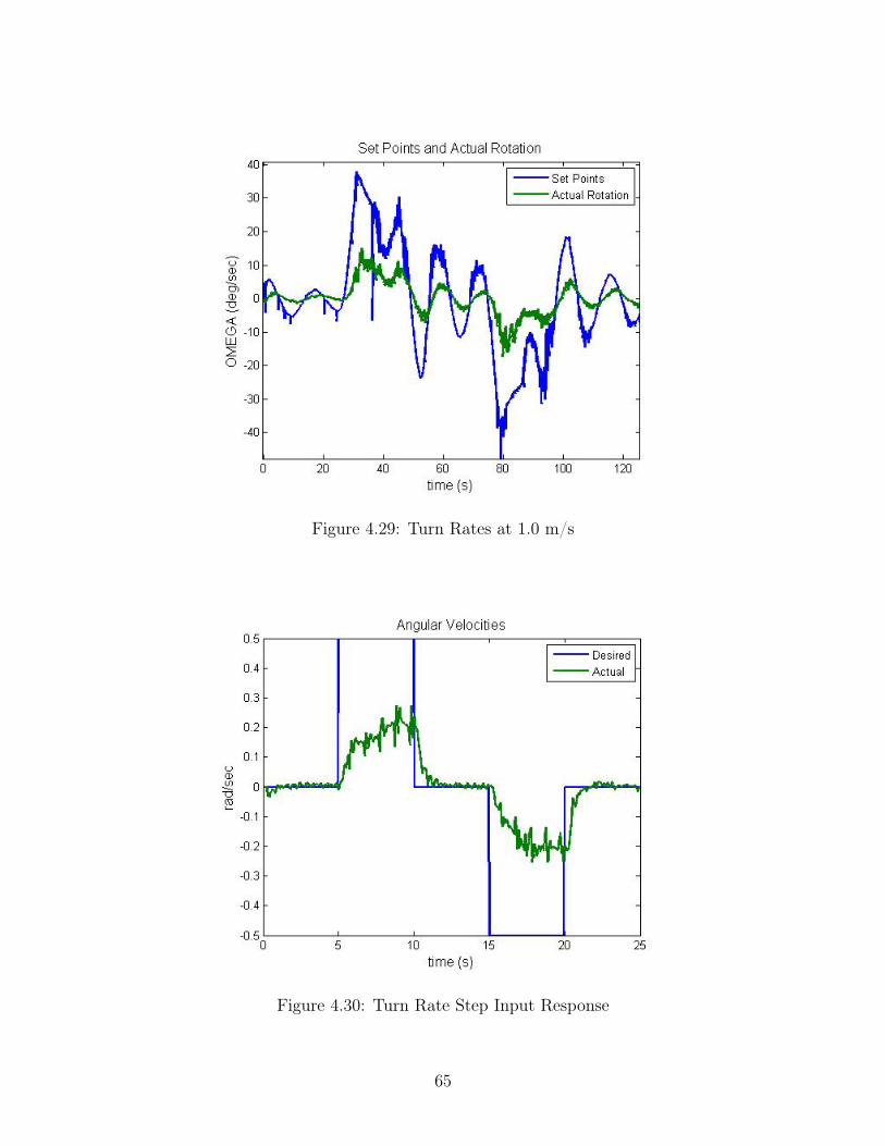
Figure 4.29: Turn Rates at 1.0 m/s
Figure 4.30: Turn Rate Step Input Response
65
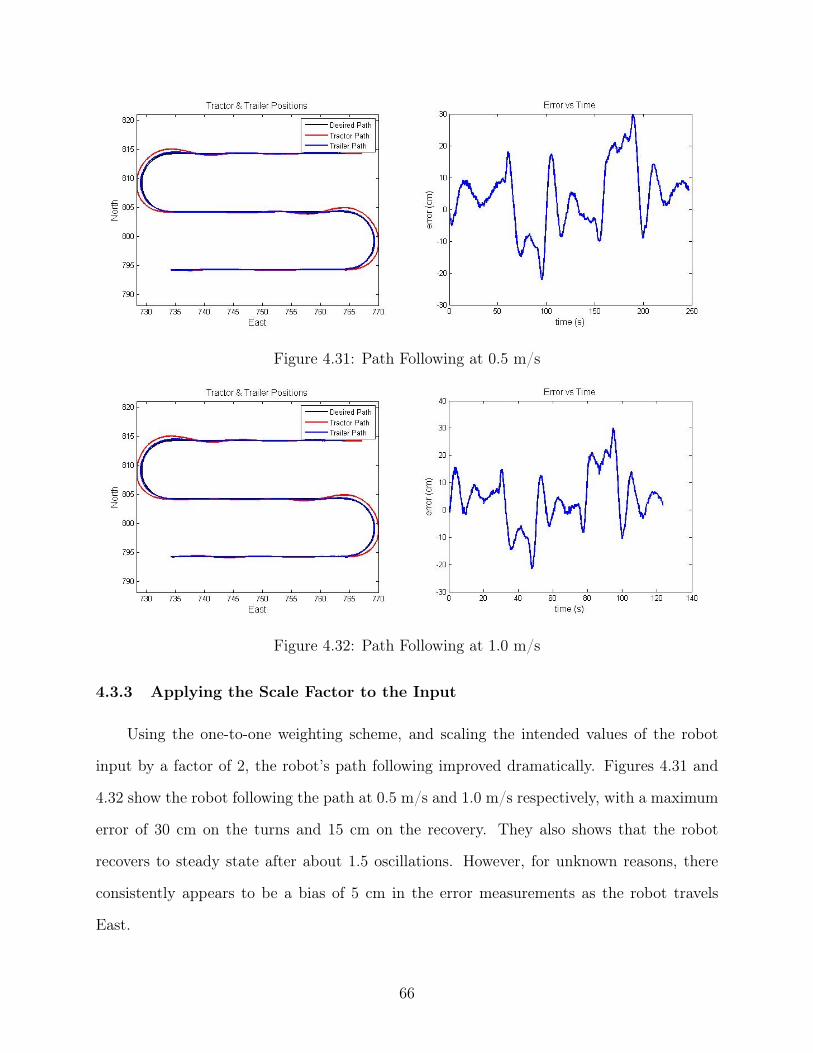
Figure 4.31: Path Following at 0.5 m/s
Figure 4.32: Path Following at 1.0 m/s
4.3.3 Applying the Scale Factor to the Input
Using the one-to-one weighting scheme, and scaling the intended values of the robot
input by a factor of 2, the robot’s path following improved dramatically. Figures 4.31 and
4.32 show the robot following the path at 0.5 m/s and 1.0 m/s respectively, with a maximum
error of 30 cm on the turns and 15 cm on the recovery. They also shows that the robot
recovers to steady state after about 1.5 oscillations. However, for unknown reasons, there
consistently appears to be a bias of 5 cm in the error measurements as the robot travels
East.
66

Figure 4.33: Path Following at 1.2 m/s
Figure 4.34: Path Following at 1.4 m/s
Next, the run was repeated using forward velocities between 1 and 2 m/s, increasing
the forward velocity in 0.2 m/s intervals. Figures 4.33 through 4.37 show how the controller
begins to lose its ability to reach steady state at 1.6 m/s.
So far, all tests have used a prediction model that assumes an immediate robot response
to a command. Further improvements might be made by factoring a first order lag with a
0.5 second time constant into the steer input of prediction model, or by designing a phase
lead compensator for the input [19].
67

Figure 4.35: Path Following at 1.6 m/s
Figure 4.36: Path Following at 1.8 m/s
Figure 4.37: Path Following at 2.0 m/s
68

4.4 Conclusion
This chapter presented the results from simulation tests in Matlab and the ROS-based
simulator, as well as results from the live run. So far, the results have shown that the perfor-
mance of this controller is comparable to the linear controller used at Auburn University. If
the system lag of the robot were factored into the model, the controller would likely perform
even better.
In addition, the results show that the horizon length and prediction weighting have
a significant effect on controller performance. Shorter horizons with heavier weighting on
the earlier predictions produce better path following on turns, but the controller tends to
overcorrect on the straight sections. Longer horizons with heavier weighting on the later pre-
dictions allow for a better recovery on the straight sections, but the path following becomes
less accurate on the turns. In future work, perhaps the controller code could be rewritten so
that the horizon length and weighting would self-adjust based on the curvature of the path
in front of the trailer, as was studied in [20].
69
Chapter 5
Summary and Conclusion
Improvements in the field of tractor-trailer control are ongoing at Auburn University.
In this thesis, the author presented a derivation of two models – a kinematic model and a
bicycle model. While the bicycle model allows for adjustments regarding turn responsiveness
and tire stiffness, the high demand on computing speed makes its feasibility questionable
using present computer technology. This could, however, change in a few years as computer
processor speeds increase.
Next, a model predictive control strategy was presented that numerically computes a
target steer angle (or turn rate for a skid-steer robot) that would keep the trailer as close
to the path as possible over a given prediction horizon. To achieve the steer angle, classical
control methods, such as a PID controller, can be applied.
The thesis concludes with simulation and experimental results, both in the lab and
in the field. First, the results of using the kinematic model for the controller against the
bicycle model were presented to simulate how the controller would react to model error.
Next, results from a live run on the Segway were presented. The simulation results showed
that the error can be as little as 8.5 cm with a highly accurate model. The live data showed
that this controller can still function with model inaccuracies, and the maximum error was
typically around 29 cm on the turns, and 15 cm on the recovery. Incorporating system lag
into the prediction model should further improve the performance of the controller, but it
will have to be considered future work.
Other future work in this field would include model validation of the bicycle tractor-
trailer model, trying the bicycle model as a control model, as well as trying different tire
models, as faster computing technology becomes available. Another way to improve the
70

Segway path following performance would be to try different skid-steer vehicle dynamic
models that account for tire slip. The overall goal is to someday use a model that produces
a highly accurate and robust control system performance without overwhelming the time
limits of the processor speed. Finding a balance between an accurate model and a reliable
control method that is fast enough to implement in real-time would enable vehicle dynamics
and control engineers to design autonomous vehicle systems to track a path to new levels of
accuracy.
71
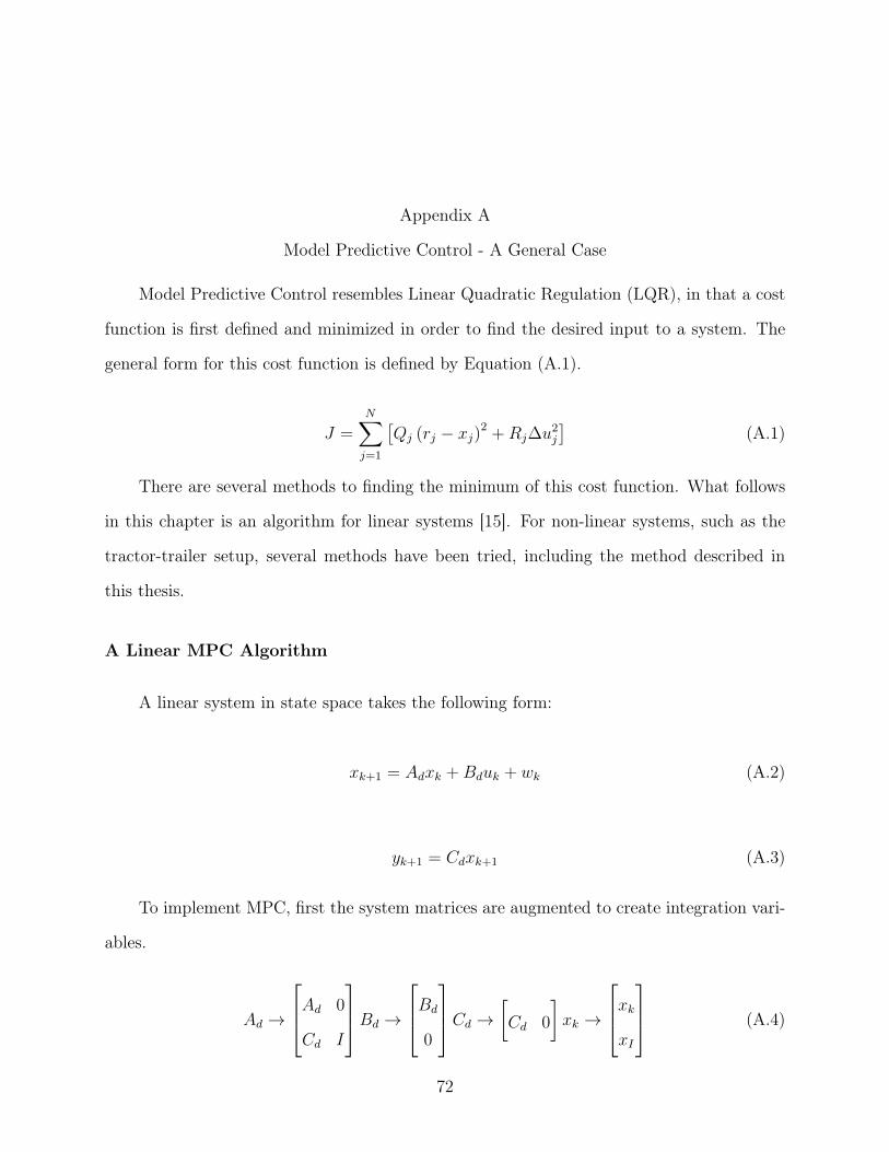
Appendix A
Model Predictive Control - A General Case
Model Predictive Control resembles Linear Quadratic Regulation (LQR), in that a cost
function is first defined and minimized in order to find the desired input to a system. The
general form for this cost function is defined by Equation (A.1).
J =
NX
j=1
⇥Q
j
(rj
� xj
)
2
+Rj
�u2
j
⇤(A.1)
There are several methods to finding the minimum of this cost function. What follows
in this chapter is an algorithm for linear systems [15]. For non-linear systems, such as the
tractor-trailer setup, several methods have been tried, including the method described in
this thesis.
A Linear MPC Algorithm
A linear system in state space takes the following form:
xk+1
= Ad
xk
+Bd
uk
+ wk
(A.2)
yk+1
= Cd
xk+1
(A.3)
To implement MPC, first the system matrices are augmented to create integration vari-
ables.
Ad
!
2
64A
d
0
Cd
I
3
75Bd
!
2
64B
d
0
3
75Cd
!C
d
0
�xk
!
2
64xk
xI
3
75 (A.4)
72

Also define:
ek
=
2
64w
k
�yref
3
75Qx
=
2
64CTQ
y
C 0
C QI
3
75Rx
= Ry
(A.5)
The predictor can be set up in a matrix format by taking a recursive approach:
xk+1|k = A
d
xk
+Bd
uk
+ wk
xk+2|k = A2
d
xk
+ Ad
Bd
uk
+Bd
uk+1|k + w
k
+ wk+1|k
...
xk+�|k = A�
d
xk
+ A��1
d
Bd
uk
+ ...+Bd
uk+��1
+ wk
+ ...+ wk+��1|k
Now, a new family of matrices can be defined:
Z =
2
66666664
Ad
A2
d
...
A�
d
3
77777775
M =
2
66666664
I 0 0 0
Ad
I 0 0
... ... I 0
A��1
d
... Ad
I
3
77777775
V = diag✓
Bd
... Bd
◆(A.6)
X =
2
66664
xk+1|k
...
xk+�|k
3
77775Xref
=
2
66664
xref
k+1|k...
xref
k+�|k
3
77775U =
2
66664
uk
...
uk+��1|k
3
77775E =
2
66664
ek
...
ek+��1|k
3
77775(A.7)
Q = diag✓Q
x
... Qx
◆R = diag
✓R
x
... Rx
◆(A.8)
The gain is computed as follows:
L =
⇣R + (MV )
T QMV⌘�1
(MV )
T Q (A.9)
73

The control input is then found:
U = �LZxk
+ Lxref � LME (A.10)
After the control input applied to the system variable k is advanced by 1, the new states
are observed, and the prediction matrix is updated:
X = Zxk
+MV U +ME (A.11)
Now, Equations (A.9), (A.10), and (A.11) may be repeated indefinitely, or until the
desired state is achieved.
74
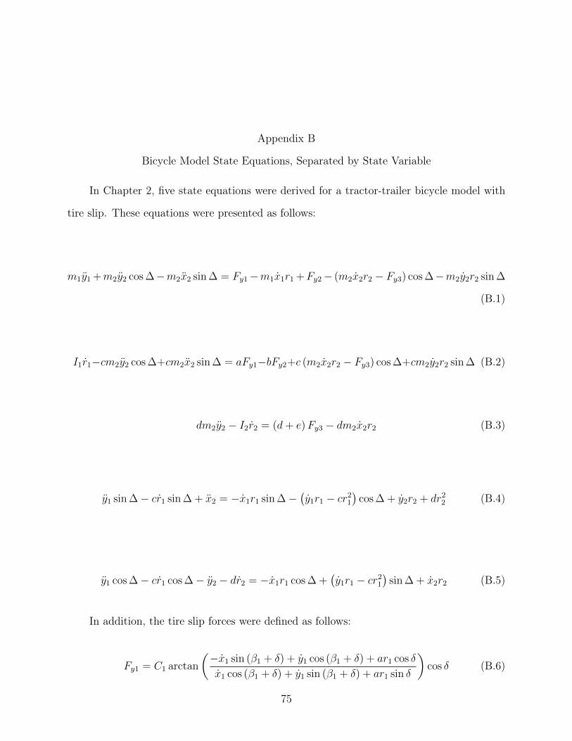
Appendix B
Bicycle Model State Equations, Separated by State Variable
In Chapter 2, five state equations were derived for a tractor-trailer bicycle model with
tire slip. These equations were presented as follows:
m1
y1
+m2
y2
cos��m2
x2
sin� = Fy1
�m1
x1
r1
+Fy2
� (m2
x2
r2
� Fy3
) cos��m2
y2
r2
sin�
(B.1)
I1
r1
�cm2
y2
cos�+cm2
x2
sin� = aFy1
�bFy2
+c (m2
x2
r2
� Fy3
) cos�+cm2
y2
r2
sin� (B.2)
dm2
y2
� I2
r2
= (d+ e)Fy3
� dm2
x2
r2
(B.3)
y1
sin�� cr1
sin�+ x2
= �x1
r1
sin���y1
r1
� cr21
�cos�+ y
2
r2
+ dr22
(B.4)
y1
cos�� cr1
cos�� y2
� dr2
= �x1
r1
cos�+
�y1
r1
� cr21
�sin�+ x
2
r2
(B.5)
In addition, the tire slip forces were defined as follows:
Fy1
= C1
arctan
✓�x
1
sin (�1
+ �) + y1
cos (�1
+ �) + ar1
cos �
x1
cos (�1
+ �) + y1
sin (�1
+ �) + ar1
sin �
◆cos � (B.6)
75
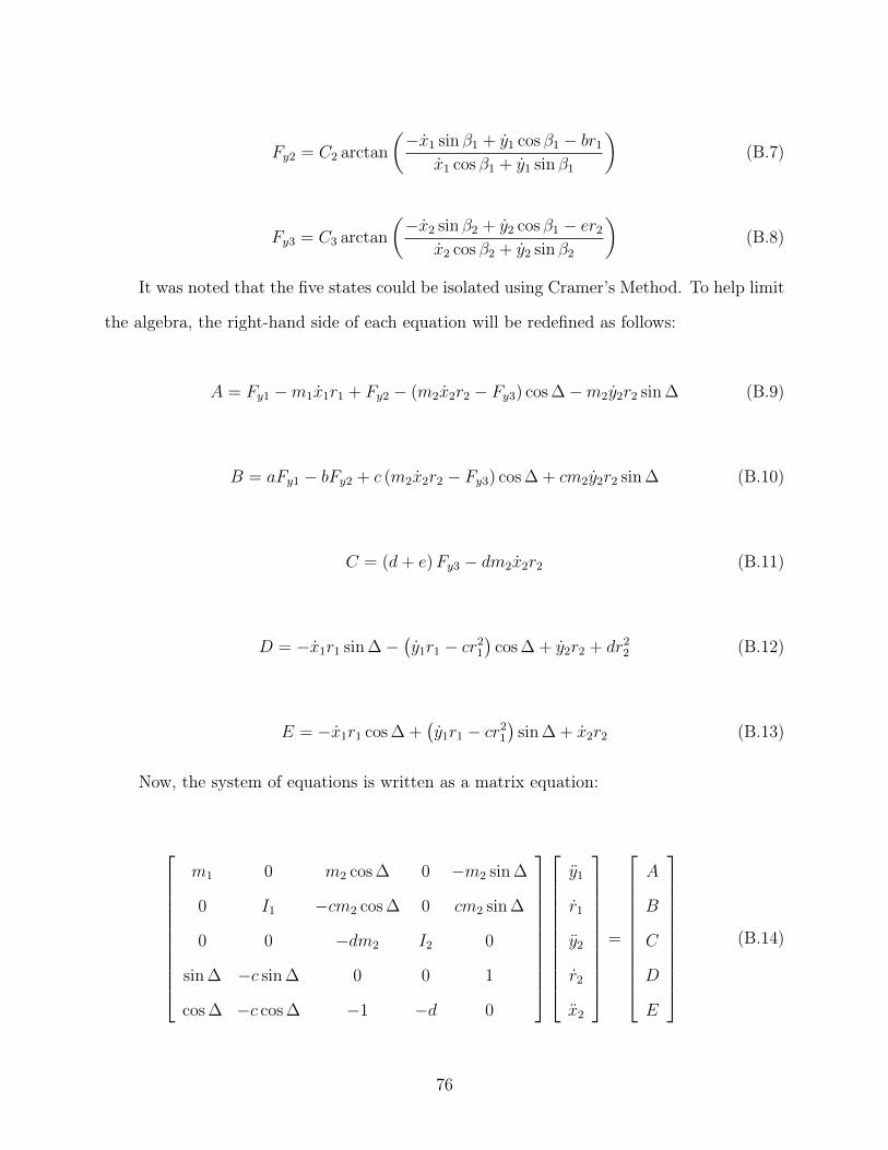
Fy2
= C2
arctan
✓�x
1
sin �1
+ y1
cos �1
� br1
x1
cos �1
+ y1
sin �1
◆(B.7)
Fy3
= C3
arctan
✓�x
2
sin �2
+ y2
cos �1
� er2
x2
cos �2
+ y2
sin �2
◆(B.8)
It was noted that the five states could be isolated using Cramer’s Method. To help limit
the algebra, the right-hand side of each equation will be redefined as follows:
A = Fy1
�m1
x1
r1
+ Fy2
� (m2
x2
r2
� Fy3
) cos��m2
y2
r2
sin� (B.9)
B = aFy1
� bFy2
+ c (m2
x2
r2
� Fy3
) cos�+ cm2
y2
r2
sin� (B.10)
C = (d+ e)Fy3
� dm2
x2
r2
(B.11)
D = �x1
r1
sin���y1
r1
� cr21
�cos�+ y
2
r2
+ dr22
(B.12)
E = �x1
r1
cos�+
�y1
r1
� cr21
�sin�+ x
2
r2
(B.13)
Now, the system of equations is written as a matrix equation:
2
66666666664
m1
0 m2
cos� 0 �m2
sin�
0 I1
�cm2
cos� 0 cm2
sin�
0 0 �dm2
I2
0
sin� �c sin� 0 0 1
cos� �c cos� �1 �d 0
3
77777777775
2
66666666664
y1
r1
y2
r2
x2
3
77777777775
=
2
66666666664
A
B
C
D
E
3
77777777775
(B.14)
76
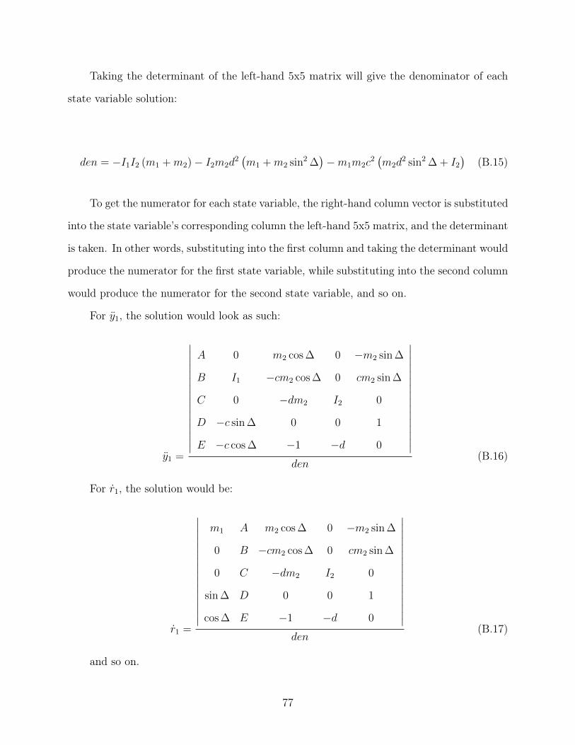
Taking the determinant of the left-hand 5x5 matrix will give the denominator of each
state variable solution:
den = �I1
I2
(m1
+m2
)� I2
m2
d2�m
1
+m2
sin
2
�
��m
1
m2
c2�m
2
d2 sin2
�+ I2
�(B.15)
To get the numerator for each state variable, the right-hand column vector is substituted
into the state variable’s corresponding column the left-hand 5x5 matrix, and the determinant
is taken. In other words, substituting into the first column and taking the determinant would
produce the numerator for the first state variable, while substituting into the second column
would produce the numerator for the second state variable, and so on.
For y1
, the solution would look as such:
y1
=
����������������
A 0 m2
cos� 0 �m2
sin�
B I1
�cm2
cos� 0 cm2
sin�
C 0 �dm2
I2
0
D �c sin� 0 0 1
E �c cos� �1 �d 0
����������������
den(B.16)
For r1
, the solution would be:
r1
=
����������������
m1
A m2
cos� 0 �m2
sin�
0 B �cm2
cos� 0 cm2
sin�
0 C �dm2
I2
0
sin� D 0 0 1
cos� E �1 �d 0
����������������
den(B.17)
and so on.
77

The solutions come out to be the following:
y
1
=
�A
⇥m
2
�I
1
c
2
+m
2
c
2
d
2
sin
2
�+ I
1
d
2
�+ I
1
I
2
⇤�Bm
2
c
�I
2
+m
2
d
2
sin
2
�
�� I
1
m
2
⇥(Cd+ EI
2
) cos�+D
�m
2
d
2
+ I
2
�sin�
⇤
�I
1
I
2
(m
1
+m
2
)� I
2
m
2
d
2
�m
1
+m
2
sin
2
�
��m
1
m
2
c
2
�m
2
d
2
sin
2
�+ I
2
�
(B.18)
r
1
=
�Am
2
c
�I
2
+m
2
d
2
sin
2
�
��B
⇥m
2
�I
2
+m
2
d
2
sin
2
�+m
1
d
2
�+m
1
I
2
⇤+ c
⇥(C + EI
2
m
1
m
2
) cos�+Dm
1
m
2
�I
2
+m
2
d
2
�sin�
⇤
�I
1
I
2
(m
1
+m
2
)� I
2
m
2
d
2
�m
1
+m
2
sin
2
�
��m
1
m
2
c
2
�m
2
d
2
sin
2
�+ I
2
�
(B.19)
y2 =
Cdh
m1
⇣
I1 + m2c2sin
2�
⌘
+ m2I1 sin
2�
i
+ I2nh
Bm1c � Dm2
⇣
m1c2+ I1
⌘
sin�
i
cos� +
h
Em1
⇣
I1 + c2m2 sin
2�
⌘
� I1⇣
A cos� � Em2 sin
2�
⌘io
�I1I2 (m1 + m2) � I2m2d2�
m1 + m2 sin
2�
�
� m1m2c2�
m2d2 sin
2� + I2
�
(B.20)
r
2
=
(Bm
1
m
2
cd�AI
1
m
2
d) cos�� C
⇥m
2
�m
1
c
2
+ I
1
�+ I
1
m
1
⇤� 1
2
Dm
2
2
d
�I
1
+m
1
c
2
�sin 2�+ Edm
2
⇥I
1
m
1
+
�I
1
+m
1
c
2
�m
2
sin
2
�
⇤
�I
1
I
2
(m
1
+m
2
)� I
2
m
2
d
2
�m
1
+m
2
sin
2
�
��m
1
m
2
c
2
�m
2
d
2
sin
2
�+ I
2
�
(B.21)
x
2
=
�I
2
+m
2
d
2
�(AI
1
�Bm
1
c) sin�+
1
2
(Cm
2
d+ EI
2
m
2
)
�I
1
+m
1
c
2
�sin 2��D
⇥I
1
I
2
�m
1
+m
2
cos
2
�
�+m
1
m
2
�I
1
d
2
+ I
2
c
2
cos
2
�
�⇤
�I
1
I
2
(m
1
+m
2
)� I
2
m
2
d
2
�m
1
+m
2
sin
2
�
��m
1
m
2
c
2
�m
2
d
2
sin
2
�+ I
2
�
(B.22)
78

Bibliography
[1] P. Falcone, F Borrelli, H. E. Tseng, J. Asgari, D. Hrovat. A Hierarchical Model PredictiveControl Framework for Autonomous Ground Vehicles. American Controls Conference,2008.
[2] H. H. Nelson, J. R. McDonald. Multisensor towed array detection system for UXOdetection. Geoscience and Remote Sensing, IEEE Transactions on 39.6 (2001): 1139-1145, 2001.
[3] B. Lepore, Defense Capabilities and Management. GAO-12-709R Military Base Realign-ments and Closures. Memorandum to the United States Government and AccountabilityOffice, 2012.
[4] L. Dubins. On curves of minimal length with a constraint on average curvature, and withprescribed initial and terminal positions and tangents. American Journal of Mathematics79, pp. 497-516. The Johns Hopkins University Press, 1957.
[5] D. M. Bevly, B. Parkinson Carrier-Phase Differential GPS for Control of a TractorTowed Implement. Proceedings of the 13th International Technical Meeting of the Satel-lite Division of The Institute of Navigation (ION GPS 2000) pp. 2263-2268, Salt LakeCity, UT, September 2000.
[6] T. C. Ng, J. Guzman, M. Adams. Autonomous vehicle-following systems: A virtualtrailer link model. Intelligent Robots and Systems, 2005 IEEE/RSJ International Con-ference, pp. 3057-3062, IEEE, 2005.
[7] L. Z. Wang, et al. An approximation approach of the clothoid curve defined in the interval[0, p/2] and its offset by free-form curves. Computer-Aided Design 33.14 (2001): 1049-1058, 2001.
[8] Seborg, Edgar, Mellichamp. Process Dynamics and Control, 2nd ed. Wiley 2003
[9] D. Hodo. Development of an Autonomous Mobile Robot-Trailer System for UXO Detec-tion. MS Thesis, Auburn University, 2007.
[10] M. Payne. Non-Collocated Control of an Autonomous Vehicle-Trailer System UsingState Estimation. MS Thesis, Auburn University, 2012.
[11] A. Singh. Nonlinear Control of a Robot-Trailer System Using a Hybrid Backstepping-linearizing approach. MS Thesis, Auburn University, 2012.
79

[12] D. Karnopp. Vehicle Stability. Marcel Dekker, 2004.
[13] D. Karnopp, D. Margolis. Engineering Applications of Dynamics. Wiley, 2008.
[14] L. Alexander, M. Donath, M. Hennessey, V. Morellas, C. Shankwitz. A Lateral DynamicModel of a Tractor-Trailer: Experimental Validation. University of Minnesota & theMinnesota Department of Transportation, 1996.
[15] P. Malaterre, and J. Rodellar. Design and comparison of multivariable optimal andpredictive controllers on a 2-pool irrigation canal. Journées Hispano-Françaises SystèmesIn- telligents & Contrôle Avancé, Laboratoire Européen Asso- cié, UPC Barcelona, 1996.
[16] S. Chapra, R. Canale. Numerical Methods for Engineers, 6th ed. McGraw Hill, 2010.
[17] R. Larson, B. Edwards, D. Falvo. Elementary Linear Algebra, 5th ed. Houghton MifflinCompany, 2004.
[18] D. Hodo, et. al. Morse Blender Simulator for Differential Steering Robot. Morse, 2011.
[19] W. Woodall. Low-Bandwidth Three Dimensional Mapping and Latency Reduction ModelPrediction to Improve Teleoperation of Robotic Vehicles. MS Thesis, Auburn University,2012.
[20] J. Backman, T. Oksanen, A. Visala. Nonlinear Model Predictive Trajectory Control inTractor-Trailer System for Parallel Guidance in Agricultural Field Operations. Agricon-trol, 2010.
80