Guidance for Obtaining Representative Laboratory

Analytical Subsamples from Particulate Laboratory

Samples

EPA/600/R-03/027 November 2003

Guidance for Obtaining Representative Laboratory

Analytical Subsamples from Particulate Laboratory Samples

by

Robert W. Gerlach Lockheed Martin Environmental Services

and

John M. Nocerino U.S. Environmental Protection Agency

223CMB03.RPT � 1/8/04

ii

Notice

The U.S. Environmental Protection Agency (U.S. EPA), through its Office of Research and Development (ORD), funded the work described here under GSA contract number GS-35F-4863G (Task Order Number 9T1Z006TMA to Lockheed Martin Environmental Services). It has been subjected to the Agency’s peer and administrative review and has been approved for publication as an EPA document.

iii

iv

Foreword

The basis for this document started in 1988. We were in a quality assurance research group dealing with the analysis of many different kinds of samples. Historically, the focus of our work was on the analytical method, and sampling was pretty much taken for granted. However, it soon became clear that sampling is perhaps the major source of error in the measurement process, and, potentially, sampling is an overwhelming source of error for heterogenous particulate materials, such as soils. It was also clear that classical statistical sampling theory was not adequate for such samples. Simple random sampling may work for very “homogeneous” samples, for instance, marbles of the very same size, weight, and shape where the only difference is the color of the marble. But the color of the marble is not a factor that contributes to the selection process of that marble! To be an effective sampling method, the factors that contribute to the selection process must be considered.

We knew that geostatistics offered some answers, such as the sample support (mass, volume, and orientation) and particle size (diameter) make a difference. That is only common sense. The larger the mass of the sample, the closer it should resemble the composition of the lot that it came from. But, taking ever larger (or more) samples was not a practical answer to getting a representative sample. Less intuitive may be that most of the heterogeneity should be associated with the larger particles and fragments. However, grinding an entire lot of material to dust was also not a practical alternative.

We searched for a non-conventional statistical sampling theory that actually takes into account the nature of particulate materials and, in 1989, we hit “pay dirt.” Dr. Francis Pitard offered a short course at the Colorado School of Mines on the Pierre Gy sampling theory for particulate materials. Dr. Pitard had taught this course many times before to mining students, but this was his first offering directed toward the environmental community. Although this theory was developed in the mid-1950s by the French chemist, Pierre Gy, the theory was not widely known to those outside of the mining community, and it was seemingly only put into practice by a few mining engineers where the bottom line really counts, namely, gold mining. Dr. Pitard had the foresight to see the importance of introducing this theory to the environmental sciences.

Needless to say, we came back from the short course very excited that we had found our answer. But it was a hard sell. Over the ensuing years, we were only moderately successful at transferring this technology to the environmental community so that it might be implemented. We started by sponsoring a couple of short courses given by Dr. Pitard and we distributed some technical transfer notes. Although this theory has proven itself in practice many times over in the mining industry, there has been very little published with substantiating experimental evidence for this theory (it has been virtually nonexistent in the environmental arena). The effectiveness of the Gy theory, and the extent to which it is applicable, was also not well-established for environmental samples. Therefore, we were compelled to start a research program to explore the effectiveness and the application of the Gy theory for all types of environmental samples, and, where there are limitations, to expand upon the theory. Such a research program would not only help to provide the needed (and published) experimental verification of the Gy

v

theory, but it should also give credence to the theory for those not yet convinced (and justify the application) of this theory for the environmental sciences.

We started our experimental investigations on the various Gy sampling theory errors, using fairly “uncomplicated” matrix-analyte combinations, as applied to obtaining a representative analytical subsample (the material that gets physically or chemically analyzed) from a laboratory sample (the bottle that comes to the laboratory containing the sample to be analyzed). We felt that this was the easiest place to start, using our limited resources, while still producing an impact. The weakest link, and the potential for the most error, could very well be from taking a non-representative grab sample “off the top” of the material in the laboratory sample bottle! (By the way, the Gy theory defines what a representative sample should be.) The result of our ongoing investigations is the first version of this guidance document. We welcome any (constructive) comments.

This document provides general guidelines for obtaining representative samples for the laboratory analysis of particulate materials using “correct” sampling practices and “correct” sampling devices. However, this guidance is general and is not limited to environmental samples. The analysis is also not limited to the laboratory; that is, this guidance is also applicable to samples analyzed in the field. The information in this guidance should also be useful in making reference standards as well as taking samples from reference standards. Similarly, this guidance should be of value in: monitoring laboratory performance, creating performance evaluation materials (and how to sample them), certifying laboratories, running collaborative trials, and performing method validations. For any of those undertakings, if there seems to be a lot of unexplained variability, then sampling or sample preparation may be the culprit, especially if one is dealing with heterogeneous particulate materials.

The material presented here: outlines the issues involved with sampling particulate materials, identifies the principal causes of uncertainty introduced by the sampling process, provides suggested solutions to sampling problems, and guides the user toward appropriate sample treatments. This document is not intended to be a simple “cookbook” of approved sampling practices.

The sections of this guidance document are divided into the following order of topics: background, theory, tools, observations, strategy, reporting, and a glossary. Many informative references are provided and should be consulted for more details. Unless one is familiar with the Gy sampling theory, correct sampling practices, and correct sampling devices, it is strongly recommended that one reads through this document at least once, especially the section on theory. The glossary can easily be consulted for unfamiliar terms. If one is familiar with the Gy sampling theory and is just interested in developing a sampling plan, or simply wants to answer the question, “How do I get a representative analytical subsample?”, then go ahead and jump to the section on “Proposed Strategies.” This section gives a general and somewhat extensive strategy guide for developing a sampling plan. A sampling strategy can be general, and not all of it, necessarily, has to be followed. However, a sampling plan is necessarily unique for each study. Any sampling endeavor should have some sort of sampling plan.

The basic strategic theme in this document is that if “correct” sampling practices are followed and “correct” sampling devices are used, then all of the sampling errors should become negligible, except for the minimum sampling error that is fundamental to the physical and chemical composition of the material being sampled. Since this minimum fundamental sampling error can be estimated before any sampling takes place, one can use this relative variance of the fundamental error to develop a sampling plan.

vi

At first, it may seem that following this guidance is a lot of effort just to analyze a small amount of material. And, when one is in a hurry and has a large case load, it may seem downright overwhelming. But, remember that the seemingly simple task of taking a small amount of material out of a laboratory sample bottle could possibly be the largest source of error in the whole measurement process. And not taking a representative subsample could produce meaningless results, which is at the very least a waste of resources and, at the very most, could lead to incorrect decisions.

Remember that sampling is one of those endeavors that you “get what you pay for,” at least in terms of effort. But, with the right knowledge and a good sampling plan, the effort is not necessarily that much. It pays to have a basic understanding of the theory. Become familiar with what causes the different sampling errors and how to minimize them through correct sampling practices. For example, always try to take as many random increments as you can, with a correctly designed sampling device, when preparing your subsample; and if you can only take a few increments, then you are still better off than taking a grab sample “off the top” from the sample bottle, and you will at least be aware of the consequences. Be able to specify what constitutes a representative subsample. Know what your sampling tools are capable of doing and if they can correctly select an increment. Always do a sample characterization (at least a visual inspection) first. At a minimum, always have study objectives and a sampling plan for each particular case. If possible, take a team approach when developing the study objectives and the sampling plan. Historical data or previous studies should be reviewed. And be sure to record the entire process!

An understanding of the primary sources of sampling uncertainty should prevent unwarranted claims and guide future studies toward correct sampling practices and more representative results. Best wishes with all of your sampling endeavors.

vii

viii

Acknowledgments

The authors express their gratitude to the following individuals for their useful suggestions and their timely review of this manuscript: Brian Schumacher (U.S. EPA), Evan Englund (U.S. EPA), Chuck Ramsey (EnviroStat), Patricia Smith (Alpha Stat), and Brad Venner (U.S. EPA). The authors also convey their thanks to Eric Nottingham and the U.S. EPA National Enforcement Investigation Center (NEIC) for the use of their facilities in performing many of the laboratory experiments pertinent to this guidance.

ix

x

Dedication

This sampling guidance document is dedicated to Dr. Pierre Gy to commemorate his fifty years toward the development and practice of his sampling theory and to Dr. Francis F. Pitard for his diligence in proliferating the Gy sampling theory and other theories for particulate sampling, for his lifetime of dedication to correct sampling practices, and for pointing those of us in the environmental analytical sciences in the right direction. The authors sincerely hope that this work expresses our gratitude and not our ignorance. We also dedicate this manuscript to all of those individuals that are involved with sampling heterogenous particulate material and we welcome any suggestions for improvement to this work.

xi

xii

Abstract

An ongoing research program has been established to experimentally verify the application of the Gy theory to environmental samples, which serves as a supporting basis for the material presented in this guidance. Research results from studies performed by the United States Environmental Protection Agency (U.S. EPA) have confirmed that the application of the Gy sampling theory to environmental heterogeneous particulate materials is the appropriate state-of-the-science approach for obtaining representative laboratory subsamples. This document provides general guidelines for obtaining representative subsamples for the laboratory analysis of particulate materials using the “correct” sampling practices and the “correct” sampling devices based on Gy theory. Besides providing background and theory, this document gives guidance on: sampling and comminution tools, sample characterization and assessment, developing a sampling plan using a general sampling strategy, and reporting recommendations. Considerations are given to: the constitution and the degree of heterogeneity of the material being sampled, the methods used for sample collection (including what proper tools to use), what it is that the sample is supposed to represent, the mass (sample support) of the sample needed to be representative, and the bounds of what “representative” actually means. A glossary and a comprehensive bibliography have been provided, which should be consulted for more details.

xiii

xiv

Table of Contents

Notice . . . . . . . . . . . . . . . . . . . . . . . . . . . . . . . . . . . . . . . . . . . . . . . . . . . . . . . . . . . . . . . . . . . . . . . . . . . . . iii

Foreword . . . . . . . . . . . . . . . . . . . . . . . . . . . . . . . . . . . . . . . . . . . . . . . . . . . . . . . . . . . . . . . . . . . . . . . . . . v

Acknowledgments . . . . . . . . . . . . . . . . . . . . . . . . . . . . . . . . . . . . . . . . . . . . . . . . . . . . . . . . . . . . . . . . . . . ix

Dedication . . . . . . . . . . . . . . . . . . . . . . . . . . . . . . . . . . . . . . . . . . . . . . . . . . . . . . . . . . . . . . . . . . . . . . . . . xi

Abstract . . . . . . . . . . . . . . . . . . . . . . . . . . . . . . . . . . . . . . . . . . . . . . . . . . . . . . . . . . . . . . . . . . . . . . . . . . xiii

Section 1 – Introduction . . . . . . . . . . . . . . . . . . . . . . . . . . . . . . . . . . . . . . . . . . . . . . . . . . . . . . . . . . . . . . . 1

1.1 Overview . . . . . . . . . . . . . . . . . . . . . . . . . . . . . . . . . . . . . . . . . . . . . . . . . . . . . . . . . . . . . . . . . . . 1

1.2 Purpose . . . . . . . . . . . . . . . . . . . . . . . . . . . . . . . . . . . . . . . . . . . . . . . . . . . . . . . . . . . . . . . . . . . . 3

1.3 Scope and Limitations . . . . . . . . . . . . . . . . . . . . . . . . . . . . . . . . . . . . . . . . . . . . . . . . . . . . . . . . . 4

1.4 Intended Audience and Their Responsibilities . . . . . . . . . . . . . . . . . . . . . . . . . . . . . . . . . . . . . . 4

1.5 Previous Guidance . . . . . . . . . . . . . . . . . . . . . . . . . . . . . . . . . . . . . . . . . . . . . . . . . . . . . . . . . . . . 5

1.6 The Measurement and Experiment Process . . . . . . . . . . . . . . . . . . . . . . . . . . . . . . . . . . . . . . . . . 6

1.7 Data Quality Objectives . . . . . . . . . . . . . . . . . . . . . . . . . . . . . . . . . . . . . . . . . . . . . . . . . . . . . . . . 8

1.8 Defining the Term, Sample, and Other Related Terms . . . . . . . . . . . . . . . . . . . . . . . . . . . . . . . . 9

1.8.1 Heterogeneity . . . . . . . . . . . . . . . . . . . . . . . . . . . . . . . . . . . . . . . . . . . . . . . . . . . . . . . . 12

1.8.2 Laboratory Subsampling: The Need for Sample Mass Reduction . . . . . . . . . . . . . . . . 14

Section 2 – Overview of Gy Sampling Theory . . . . . . . . . . . . . . . . . . . . . . . . . . . . . . . . . . . . . . . . . . . . 15

2.1 Background . . . . . . . . . . . . . . . . . . . . . . . . . . . . . . . . . . . . . . . . . . . . . . . . . . . . . . . . . . . . . . . . 15

2.2 Uncertainty Mechanisms . . . . . . . . . . . . . . . . . . . . . . . . . . . . . . . . . . . . . . . . . . . . . . . . . . . . . . 16

2.3 Gy Sampling Theory: Some Assumptions and Limitations . . . . . . . . . . . . . . . . . . . . . . . . . . . 16

2.4 Gy Sampling Theory: Errors . . . . . . . . . . . . . . . . . . . . . . . . . . . . . . . . . . . . . . . . . . . . . . . . . . . 17

2.5 Subsample Selection Issues . . . . . . . . . . . . . . . . . . . . . . . . . . . . . . . . . . . . . . . . . . . . . . . . . . . . 18

2.6 The Relationship Between the Gy Sampling Theory Errors . . . . . . . . . . . . . . . . . . . . . . . . . . . 19

2.7 The Short-Range Heterogeneity Fluctuation Error, CE1 . . . . . . . . . . . . . . . . . . . . . . . . . . . . . . 22

2.8 The Fundamental Error (FE) - the Heterogeneity of Particulate Constitution . . . . . . . . . . . . . . 23

2.9 The Grouping and Segregation Error (GE) - the Heterogeneity of Particle Distributions . . . . 24

2.10 The Long-Range Heterogeneity Fluctuation Error (CE2) . . . . . . . . . . . . . . . . . . . . . . . . . . . . . 27

xv

Table of Contents, Continued

2.11 The Periodic Heterogeneity Fluctuation Error (CE3) . . . . . . . . . . . . . . . . . . . . . . . . . . . . . . . . . 28

2.12 The Increment Materialization Error (ME), the Increment Delimitation Error (DE) and theIncrement Extraction Error (EE): Subsampling Tool Design and Execution . . . . . . . . . . . . . . 28

2.13 The Preparation Error (PE) – Sample Integrity . . . . . . . . . . . . . . . . . . . . . . . . . . . . . . . . . . . . . 34

2.14 The Importance of Correctly Selected Increments . . . . . . . . . . . . . . . . . . . . . . . . . . . . . . . . . . 35

2.15 Increment Sampling and Splitting Sampling . . . . . . . . . . . . . . . . . . . . . . . . . . . . . . . . . . . . . . . 37

2.16 Correct Sampling (Correct Selection) Defined . . . . . . . . . . . . . . . . . . . . . . . . . . . . . . . . . . . . . 38

2.17 Representative Sample Defined . . . . . . . . . . . . . . . . . . . . . . . . . . . . . . . . . . . . . . . . . . . . . . . . . 39

Section 3 – Fundamental Error Fundamentals . . . . . . . . . . . . . . . . . . . . . . . . . . . . . . . . . . . . . . . . . . . . . 41

3.1 Estimating the Relative Variance of the Fundamental Error, sFE 2 . . . . . . . . . . . . . . . . . . . . . . . 41

3.2 Estimating the Factors for the Relative Variance of the Fundamental Error Equation . . . . . . . 43

3.2.1 Estimating the Mineralogical (Composition) Factor, c . . . . . . . . . . . . . . . . . . . . . . . . . 43

3.2.2 Estimating the Liberation Factor, l . . . . . . . . . . . . . . . . . . . . . . . . . . . . . . . . . . . . . . . . 44

3.2.3 Estimating the Shape Factor, f . . . . . . . . . . . . . . . . . . . . . . . . . . . . . . . . . . . . . . . . . . . . 45

3.2.4 Estimating the Granulometric Factor, g . . . . . . . . . . . . . . . . . . . . . . . . . . . . . . . . . . . . . 46

3.2.5 Estimating the Nominal Particle Size, d . . . . . . . . . . . . . . . . . . . . . . . . . . . . . . . . . . . . 47

3.2.6 Estimating the Required Sample Mass, Ms . . . . . . . . . . . . . . . . . . . . . . . . . . . . . . . . . . 47

3.2.7 Rearrangement of the Relative Variance for the Fundamental Error Equation toDetermine the Sample Mass (Ms) . . . . . . . . . . . . . . . . . . . . . . . . . . . . . . . . . . . . . . . . . 47

3.2.8 Two-tiered Variance Comparison to Estimate IHL and the Sample Mass (Ms) . . . . . . . 48

3.2.9 Visman Sampling Constants Approach for Determining the Sample Mass (Ms) . . . . . 50

3.3 Developing a Sample Mass or Comminution Strategy: The Sampling Nomograph . . . . . . . . 50

3.3.1 Constructing a Sampling Nomograph . . . . . . . . . . . . . . . . . . . . . . . . . . . . . . . . . . . . . . 51

3.3.2 Hypothetical Example . . . . . . . . . . . . . . . . . . . . . . . . . . . . . . . . . . . . . . . . . . . . . . . . . . 53

3.3.3 Some Subsampling Strategy Points to Consider . . . . . . . . . . . . . . . . . . . . . . . . . . . . . . 56

3.4 Low Analyte Concentration Considerations . . . . . . . . . . . . . . . . . . . . . . . . . . . . . . . . . . . . . . . 57

3.4.1 Low-frequency of Analyte (Contaminant) Particles . . . . . . . . . . . . . . . . . . . . . . . . . . . 57

3.4. 22 A Low Concentration Approximation of sFE . . . . . . . . . . . . . . . . . . . . . . . . . . . . . . . . 58

3.4.3 A Simplified Low Concentration Approximation of sFE 2 . . . . . . . . . . . . . . . . . . . . . . . 59

Section 4 – Subsampling Techniques . . . . . . . . . . . . . . . . . . . . . . . . . . . . . . . . . . . . . . . . . . . . . . . . . . . 61

4.1 Subsampling Methods . . . . . . . . . . . . . . . . . . . . . . . . . . . . . . . . . . . . . . . . . . . . . . . . . . . . . . . . 61

4.1.1 Sectorial Splitter . . . . . . . . . . . . . . . . . . . . . . . . . . . . . . . . . . . . . . . . . . . . . . . . . . . . . . 61

4.1.1.1 Advantages . . . . . . . . . . . . . . . . . . . . . . . . . . . . . . . . . . . . . . . . . . . . . . . . . . . 62

xvi

Table of Contents, Continued

4.1.1.2 Disadvantages . . . . . . . . . . . . . . . . . . . . . . . . . . . . . . . . . . . . . . . . . . . . . . . . . 62

4.1.2 Paper Cone Sectorial Splitting . . . . . . . . . . . . . . . . . . . . . . . . . . . . . . . . . . . . . . . . . . . . 62

4.1.3 Incremental Sampling . . . . . . . . . . . . . . . . . . . . . . . . . . . . . . . . . . . . . . . . . . . . . . . . . . 63

4.1.4 Riffle Splitting . . . . . . . . . . . . . . . . . . . . . . . . . . . . . . . . . . . . . . . . . . . . . . . . . . . . . . . . 64

4.1.5 Alternate Shoveling . . . . . . . . . . . . . . . . . . . . . . . . . . . . . . . . . . . . . . . . . . . . . . . . . . . . 65

4.1.6 Coning and Quartering . . . . . . . . . . . . . . . . . . . . . . . . . . . . . . . . . . . . . . . . . . . . . . . . . 65

4.1.7 Rolling and Quartering . . . . . . . . . . . . . . . . . . . . . . . . . . . . . . . . . . . . . . . . . . . . . . . . . 66

4.1.8 Fractional Shoveling . . . . . . . . . . . . . . . . . . . . . . . . . . . . . . . . . . . . . . . . . . . . . . . . . . . 66

4.1.9 Degenerate Fractional Shoveling . . . . . . . . . . . . . . . . . . . . . . . . . . . . . . . . . . . . . . . . . . 67

4.1.10 Table Sampler . . . . . . . . . . . . . . . . . . . . . . . . . . . . . . . . . . . . . . . . . . . . . . . . . . . . . . . . 68

4.1.11 V-Blender . . . . . . . . . . . . . . . . . . . . . . . . . . . . . . . . . . . . . . . . . . . . . . . . . . . . . . . . . . . 68

4.1.12 Vibratory Spatula . . . . . . . . . . . . . . . . . . . . . . . . . . . . . . . . . . . . . . . . . . . . . . . . . . . . . . 69

4.1.13 Grab Sampling . . . . . . . . . . . . . . . . . . . . . . . . . . . . . . . . . . . . . . . . . . . . . . . . . . . . . . . . 69

4.2 Minimizing Particle and Mass Fragment Correlation . . . . . . . . . . . . . . . . . . . . . . . . . . . . . . . . 69

4.3 Ranking Subsampling Methods . . . . . . . . . . . . . . . . . . . . . . . . . . . . . . . . . . . . . . . . . . . . . . . . . 70

Section 5 – Comminution (Particle Size Reduction) Methods . . . . . . . . . . . . . . . . . . . . . . . . . . . . . . . . 73

Section 6 – Sample Characterization and Assessment . . . . . . . . . . . . . . . . . . . . . . . . . . . . . . . . . . . . . . . 75

6.1 Identifying Important Sample Characteristics . . . . . . . . . . . . . . . . . . . . . . . . . . . . . . . . . . . . . . 75

6.2 Visual Characteristics . . . . . . . . . . . . . . . . . . . . . . . . . . . . . . . . . . . . . . . . . . . . . . . . . . . . . . . . 76

6.2.1 Analyte Particles: Color, Texture, Shape, and Number . . . . . . . . . . . . . . . . . . . . . . . . 76

6.2.2 Unique or Special Features . . . . . . . . . . . . . . . . . . . . . . . . . . . . . . . . . . . . . . . . . . . . . . 77

6.2.3 Density . . . . . . . . . . . . . . . . . . . . . . . . . . . . . . . . . . . . . . . . . . . . . . . . . . . . . . . . . . . . . . 77

6.3 Moisture Content and Thermally Sensitive Materials . . . . . . . . . . . . . . . . . . . . . . . . . . . . . . . . 77

6.4 Particle Size, Classification, and Screening Decisions . . . . . . . . . . . . . . . . . . . . . . . . . . . . . . . 78

6.5 Concentration Distribution . . . . . . . . . . . . . . . . . . . . . . . . . . . . . . . . . . . . . . . . . . . . . . . . . . . . 80

6.6 Comminution (Grinding and Crushing) . . . . . . . . . . . . . . . . . . . . . . . . . . . . . . . . . . . . . . . . . . . 80

6.6.1 Caveats . . . . . . . . . . . . . . . . . . . . . . . . . . . . . . . . . . . . . . . . . . . . . . . . . . . . . . . . . . . . . 81

Section 7 – Proposed Strategies . . . . . . . . . . . . . . . . . . . . . . . . . . . . . . . . . . . . . . . . . . . . . . . . . . . . . . . . 83

7.1 The Importance of Historical and Preliminary Information . . . . . . . . . . . . . . . . . . . . . . . . . . . 85

7.2 A Generic Strategy to Formulate an Analytical Subsampling Plan . . . . . . . . . . . . . . . . . . . . . . 86

7.3 An Example Quick Estimate Protocol . . . . . . . . . . . . . . . . . . . . . . . . . . . . . . . . . . . . . . . . . . . . 91

xvii

Table of Contents, Continued

Section 8 – Case Studies . . . . . . . . . . . . . . . . . . . . . . . . . . . . . . . . . . . . . . . . . . . . . . . . . . . . . . . . . . . . . 93

8.1 Case Study: Increment Subsampling and Sectorial Splitting Subsampling . . . . . . . . . . . . . . . 93

8.2 Case Study: The Effect of a Few Large Particles on the Uncertainty from Sampling . . . . . . . 95

8.3 Case Study: Sampling Uncertainty Due to Contaminated Particles with Different Size Fractions . . . . . . . . . . . . . . . . . . . . . . . . . . . . . . . . . . . . . . . . . . . . . . . . . . . . . . . . 96

8.4 Case Study: The Relative Variance of the Fundamental Error and Two Components . . . . . . . 96

8.5 Case Study: IHL Example . . . . . . . . . . . . . . . . . . . . . . . . . . . . . . . . . . . . . . . . . . . . . . . . . . . . . 97

8.6 Case Study: Selecting a Fraction Between Two Screens . . . . . . . . . . . . . . . . . . . . . . . . . . . . . 98

8.7 Case Study: Subsampling Designs . . . . . . . . . . . . . . . . . . . . . . . . . . . . . . . . . . . . . . . . . . . . . 100

8.7.1 Subsampling Design A . . . . . . . . . . . . . . . . . . . . . . . . . . . . . . . . . . . . . . . . . . . . . . . . 101

8.7.2 Subsampling Design B . . . . . . . . . . . . . . . . . . . . . . . . . . . . . . . . . . . . . . . . . . . . . . . . 101

8.7.3 Subsampling Design C . . . . . . . . . . . . . . . . . . . . . . . . . . . . . . . . . . . . . . . . . . . . . . . . 102

8.7.4 Subsampling Design D . . . . . . . . . . . . . . . . . . . . . . . . . . . . . . . . . . . . . . . . . . . . . . . . 103

8.8 Case Study: Subsampling Designs Summary . . . . . . . . . . . . . . . . . . . . . . . . . . . . . . . . . . . . . 103

Section 9 – Reporting Results . . . . . . . . . . . . . . . . . . . . . . . . . . . . . . . . . . . . . . . . . . . . . . . . . . . . . . . . 105

9.1 Introduction . . . . . . . . . . . . . . . . . . . . . . . . . . . . . . . . . . . . . . . . . . . . . . . . . . . . . . . . . . . . . . . 105

9.2 For the Analyst . . . . . . . . . . . . . . . . . . . . . . . . . . . . . . . . . . . . . . . . . . . . . . . . . . . . . . . . . . . . 106

9.3 For the Scientists and Statisticians . . . . . . . . . . . . . . . . . . . . . . . . . . . . . . . . . . . . . . . . . . . . . . 108

9.4 For the Managers . . . . . . . . . . . . . . . . . . . . . . . . . . . . . . . . . . . . . . . . . . . . . . . . . . . . . . . . . . . 109

9.5 For the Decision Makers . . . . . . . . . . . . . . . . . . . . . . . . . . . . . . . . . . . . . . . . . . . . . . . . . . . . . 110

Section 10 – Summary and Conclusions . . . . . . . . . . . . . . . . . . . . . . . . . . . . . . . . . . . . . . . . . . . . . . . . 111

Recommendations . . . . . . . . . . . . . . . . . . . . . . . . . . . . . . . . . . . . . . . . . . . . . . . . . . . . . . . . . . . . . . . . . 113

References . . . . . . . . . . . . . . . . . . . . . . . . . . . . . . . . . . . . . . . . . . . . . . . . . . . . . . . . . . . . . . . . . . . . . . . 115

Bibliography . . . . . . . . . . . . . . . . . . . . . . . . . . . . . . . . . . . . . . . . . . . . . . . . . . . . . . . . . . . . . . . . . . . . . 119

Glossary of Terms . . . . . . . . . . . . . . . . . . . . . . . . . . . . . . . . . . . . . . . . . . . . . . . . . . . . . . . . . . . . . . . . . 125

xviii

List of Figures

Figure # Description Page

1 The experiment and measurement process . . . . . . . . . . . . . . . . . . . . . . . . . . . . . . . . . . . . . . 7

2 A depiction of the sample acquisition process . . . . . . . . . . . . . . . . . . . . . . . . . . . . . . . . . . . 12

3 Contour plot of contaminant level across a hazardous waste site . . . . . . . . . . . . . . . . . . . . 17

4 A depiction of the fundamental error (FE) . . . . . . . . . . . . . . . . . . . . . . . . . . . . . . . . . . . . . 23

5 The grouping and segregation error (GE) . . . . . . . . . . . . . . . . . . . . . . . . . . . . . . . . . . . . . . 25

6 The effect of sample size when there are few analyte particles . . . . . . . . . . . . . . . . . . . . . . 26

7 The increment delimitation error (DE) . . . . . . . . . . . . . . . . . . . . . . . . . . . . . . . . . . . . . . . . 29

8 Increments selected with incorrect and correct devices . . . . . . . . . . . . . . . . . . . . . . . . . . . . 30

9 Correct and incorrect increment delimitation when sampling from a moving belt . . . . . . . 31

10 (a) Delimitation for the extended increment . . . . . . . . . . . . . . . . . . . . . . . . . . . . . . . . . . . . 32

(b) Ideal increment extraction . . . . . . . . . . . . . . . . . . . . . . . . . . . . . . . . . . . . . . . . . . . . . . . 32

(c) An increment extraction error (EE) can occur when particles cross the extendedincrement boundary . . . . . . . . . . . . . . . . . . . . . . . . . . . . . . . . . . . . . . . . . . . . . . . . . . . . 32

(d) Delimitation for the extended increment for a cylindrical sampling device for a two-dimensional sample . . . . . . . . . . . . . . . . . . . . . . . . . . . . . . . . . . . . . . . . . . . . . . . . . . . . 32

(e) The particles that get extracted into the increment have their center of gravity withinthe extended increment boundary of the sampling device . . . . . . . . . . . . . . . . . . . . . . . 32

11 For correct increment extraction, the shape of the sampling device's cutting edges mustbe designed with respect to the center of gravity of the particle and its chance to be partof the sample or part of the rejects . . . . . . . . . . . . . . . . . . . . . . . . . . . . . . . . . . . . . . . . . . . . 33

12 This highly segregated lot is randomly sampled with increments of the same total area . . 37

13 An example of a sampling nomograph . . . . . . . . . . . . . . . . . . . . . . . . . . . . . . . . . . . . . . . . 52

14 A sectorial splitter with eight sectors . . . . . . . . . . . . . . . . . . . . . . . . . . . . . . . . . . . . . . . . . . 54

15 A paper cone sectorial splitter with eight sectors . . . . . . . . . . . . . . . . . . . . . . . . . . . . . . . . 62

16 A riffle splitter with 20 chutes and two collection pans . . . . . . . . . . . . . . . . . . . . . . . . . . . 64

xix

List of Figures, Continued

17 The alternate shoveling procedure . . . . . . . . . . . . . . . . . . . . . . . . . . . . . . . . . . . . . . . . . . . . 65

18 The coning and quartering procedure . . . . . . . . . . . . . . . . . . . . . . . . . . . . . . . . . . . . . . . . . 65

19 The fractional shoveling procedure . . . . . . . . . . . . . . . . . . . . . . . . . . . . . . . . . . . . . . . . . . . 67

20 The degenerate fractional shoveling procedure . . . . . . . . . . . . . . . . . . . . . . . . . . . . . . . . . . 67

21 A table sampler . . . . . . . . . . . . . . . . . . . . . . . . . . . . . . . . . . . . . . . . . . . . . . . . . . . . . . . . . . 68

22 A V-blender . . . . . . . . . . . . . . . . . . . . . . . . . . . . . . . . . . . . . . . . . . . . . . . . . . . . . . . . . . . . . 68

23 (a) Sample estimate bias and cumulative bias versus run number for theincremental subsampling runs . . . . . . . . . . . . . . . . . . . . . . . . . . . . . . . . . . . . . . . . . . . . 94

(b) Sample estimate bias and cumulative bias versus run number for the sectorialsampling runs . . . . . . . . . . . . . . . . . . . . . . . . . . . . . . . . . . . . . . . . . . . . . . . . . . . . . . . . 94

xx

List of Tables

Table # Description Page

1 The seven steps in the DQO process . . . . . . . . . . . . . . . . . . . . . . . . . . . . . . . . . . . . . . . . . . . 8

2 Gy sampling theory error types for particulate materials . . . . . . . . . . . . . . . . . . . . . . . . . . 18

3 Mechanisms for increased bias and variability due to sample integrity and the PE . . . . . . 35

4 Liberation parameter estimates by material description . . . . . . . . . . . . . . . . . . . . . . . . . . . 45

5 Examples of shape parameters . . . . . . . . . . . . . . . . . . . . . . . . . . . . . . . . . . . . . . . . . . . . . . . 46

6 Granulometric factor values identified by Gy (1998) . . . . . . . . . . . . . . . . . . . . . . . . . . . . . 47

7 The relationship of the particle diameter, the analyte concentration, and the desireduncertainty level to the sample mass . . . . . . . . . . . . . . . . . . . . . . . . . . . . . . . . . . . . . . . . . . 60

8 Authors’ relative rankings (from best to worst) for subsampling methods . . . . . . . . . . . . . 72

9 Soil particle classes by particle size, and classification names for soil fragments fromclay to boulders . . . . . . . . . . . . . . . . . . . . . . . . . . . . . . . . . . . . . . . . . . . . . . . . . . . . . . . . . . 79

10 The minimum sample mass, Ms, and the maximum particle size, d, for sFE # 15%(density = 2.5, analyte weight proportion = 0.05) . . . . . . . . . . . . . . . . . . . . . . . . . . . . . . . . 81

11 The influence of particle size on uncertainty . . . . . . . . . . . . . . . . . . . . . . . . . . . . . . . . . . . . 96

12 Case study: IHL example parameters . . . . . . . . . . . . . . . . . . . . . . . . . . . . . . . . . . . . . . . . . 98

13 Case study: Parameters for selecting a fraction between two screens . . . . . . . . . . . . . . . . 99

14 A summary of the results from the case study designs . . . . . . . . . . . . . . . . . . . . . . . . . . . 104

xxi

Section 1

Introduction

Please note that there is a glossary in the back of this guidance document that should help the reader understand unfamiliar words or concepts. For more extensive explanations of sampling topics that are not covered in this text, please refer to the bibliography.

1.1 Overview

Unless a heterogeneous population (for example: a material, a product, a lot, or a contaminated site) can be completely and exhaustively measured or analyzed, sampling is the first physical step in any measurement process or experimental study of that population. The characteristics of collected samples are used to make estimates of the characteristics of the population; thus, samples are used to infer properties about the population in order to formulate new hypotheses, deduce conclusions, and implement decisions about the population. The assumption is that the samples both accurately and precisely represent the population. Without special attention to that assumption, sampling could be the weakest link leading to the largest errors in the measurement process or the experimental study.

Sampling plays an especially important role in environmental studies and decisions. In most environmental studies, field samples (often specimens) are collected from various field locations. The characteristics measured in those samples and any consequent subsamples (a sample of a sample), including laboratory subsamples, are then considered, de facto, as being “representative” of the site from which they were collected. However, just because a sample comes from the site under consideration, it does not mean that the sample represents that site. Considerations must be given about the constitution of the material being sampled, the degree of heterogeneity of the material being sampled, the methods used for sample collection (including what proper tools to use), what it is that the sample is supposed to represent, the mass (sample support) of the sample needed to be representative, and the bounds of what “representative” actually means. If a collection of samples does not represent the population from which they are drawn, then the statistical analyses of the generated data may lead to misinformed conclusions and consequent (and perhaps costly) decisions.

Technical issues related to subsampling seem to fall into a gap between the concerns about the number and location of field samples (e.g., in a field sampling plan) and the concerns about the performance of an analytical method for individual subsamples. This is partly because subsampling is viewed as a transitional event that often appears trivial compared to the field activity and laboratory

Everything should be made as simple as possible, but not simpler.

- Albert Einstein

Page 1 of 134

analysis steps on either end of the measurement process. Hence, subsampling is rarely evaluated to assess its effect on subsequent analysis steps or on decisions based on the results.

But, the error introduced by subsampling should not be ignored. The uncertainty associated with this activity can exceed analytical method uncertainties by an order of magnitude or more (Jenkins et al., 1997; and Gerlach et al., 2002). Biased results from incorrect sample mass reduction methods can negate the influence of the best field sampling designs for sample location, number, and type. Improper subsampling can lead to highly variable and biased analytical results that are not amenable to control through standard quality control measures. This can cause misleading results for decision makers relying on measurement results to support corrective actions.

Any lot (e.g., a site, a section from a site, or a batch) of particulate material consists of particles having diverse characteristics with respect to size, shape, density, distribution, as well as physical and chemical constitution. This diversity in the particle properties, the lot-specific uniqueness of the distribution of the analytes of interest, and the uncertainties due to the subsampling techniques in the field and the laboratory, often lead to a large variability among the analytical results of the samples that are supposed to represent the lot.

Correct subsampling requires an understanding of those particulate material characteristics for the population under study (e.g., a lot, a site, a sample) and the technical decisions that the results are intended to support. The sample features, as well as the reasons for sampling, guide the sampler in identifying the sampling activities that are helpful and avoid sampling actions that can lead to increased bias and uncertainty.

A collected sample must be both accurate and precise, within set specifications, at the same time in order to be representative of the lot. This is true not only for the collection of the primary (or field) sample, but also of any sample reduction or subsampling step. Such steps include sample preparation, comminution (crushing or grinding), “homogenization,” blending, weighing, and other mass reductions or the splitting of samples. Taking out a portion of material from the laboratory sample bottle for weighing and analysis (the analytical subsample) is a sample mass reduction step and should be performed with “correct” subsampling practices in order to get a representative result. Laboratory subsampling errors (e.g., incorrectly taking an aliquot from a sample bottle for analysis) could potentially overwhelm other errors, including other sampling steps and the analytical error, associated with the analyses of samples. It is quite a “lot” to ask of the tiny (on the order of a few grams, and often much lower) laboratory analytical subsample to be representative of each of the larger and larger (parent) samples in the chain from which it was derived, up to the entire lot (which could be many tons). Therefore, it is imperative that each subsample is as representative as possible of the parent sample from which it is derived. Any subsampling error is only going to propagate down the chain from the largest sample to the smallest laboratory analytical subsample.

Page 2 of 134

1.2 Purpose

This guidance is a product of the ongoing research in our chemometrics program to improve or develop methods to reduce data uncertainty in the measurement or experiment process. Since sampling is usually a very early stage in that process, we searched for ways to reduce sampling errors and obtain representative samples for particulate materials. Fortunately, there is an extensive and complete sampling theory, known as the Pierre Gy sampling theory, developed mainly for the mining industry, that addresses the issue of obtaining representative samples from particulate materials. Although this theory has proven itself in practice in the mining industry, very little evidence exists in the literature that verifies this theory experimentally, and this theory has only recently received attention for environmental studies. Our goals are to verify Gy sampling theory experimentally for environmental particulate samples, discover any limitations in the theory for such samples, and to develop extensions to the theory if such limitations exist.

Since the laboratory subsample can potentially have the greatest error in representing the lot and because of its manageable size and relative simplicity (the long-range “field” type heterogeneities can be regarded as trivial), we focused our initial experimental studies, and this ensuing guidance, on using “correct” sampling methods to obtain “representative” laboratory analytical subsamples of particulate materials. The terms, “correct” and “representative,” will be used as defined by Francis Pitard (Pitard, 1993) and they will be described in detail in this document.

One of the main purposes of this document is to present a general subsampling strategy. Based on that strategy, individual sampling plans may then be developed for each unique case that should produce representative analytical subsamples by following correct sampling practices. By following correct sampling practices, all of the “controllable” sampling biases and relative variances defined by the Gy sampling theory should be minimized such that a representative subsample can simply be defined by the relative variance of just one sampling error, the fundamental error (FE). This is the minimum and “natural” relative variance associated with the lot (for our purposes, the primary laboratory sample from which a representative analytical subsample is to be taken), and is based on the physical and chemical characteristics and composition of the particulate materials (and other items) that make up that lot. Those chemical and physical differences between the different items of the lot material are due to the constitution heterogeneity (CH). The Gy sampling theory can quantify this relative variance of thefundamental error (s FE

2) through an equation based on the chemical and physical characteristics of thelot. Hence, we can estimate what the s 2 should be for the analytical subsample, and, therefore, shouldFE

be able to develop a strategy to obtain a representative analytical subsample a priori – that is, before engaging in the subsampling operation – simply based on observations about the chemical and physical characteristics of the lot!

Thus, this guidance identifies the subsampling activities that minimize biased or highly variable results. This guidance also suggests which practices to avoid. Provided in this document is a general introduction to subsampling, followed by specific suggestions and proposed laboratory subsampling procedures. This guidance focuses on a strategy to minimize uncertainty through the use of correct sampling techniques to obtain representative samples.

Page 3 of 134

1.3 Scope and Limitations

This guidance is not intended as a guide for field sampling at a hazardous waste site. The Agency has developed a series of documents to assist in that process (see U.S. EPA 1994, 1996a-c, 1997, 1998, and 2000a-d). Correct sampling practices to obtain representative field samples is the subject of ongoing research and a future guidance document.

Instead, the primary focus of this guidance document is on identifying ways to obtain representative laboratory analytical subsamples, the ideal subsample being one with characteristics identical to the original laboratory sample. This document provides guidance on the laboratory sample processing and mass reduction methods associated with laboratory analytical subsampling practices. Laboratory subsampling takes place every time an analyst selects an analytical subsample from a laboratory sample. (This guidance is general and is not limited to environmental samples; it also applies to selecting field analytical subsamples.)

This guidance focuses on the issues and actions related to samples composed of particulate materials. It is not intended for samples selected for analysis of volatile or reactive constituents, and it does not extend to sampling biological materials, aqueous samples, or viscous materials such as grease or oil trapped in a particulate matrix, e.g., crude oil in beach aggregate. Research into the correct sampling of those analytes and matrices is ongoing and guidance will be prepared once research results provide a foundation for appropriate practices.

This guidance is intended as a technical resource for individuals who select subsamples for analysis or other purposes, such as those individuals directing others in this activity. It also contains information of interest to anyone else that deals with the subsampling of particulate material in a secondary manner, including anyone reviewing study results from the analysis of particulate samples. Examples and discussions relevant to these issues can be found in a number of the references. The following references contain extensive or particularly valuable material on the topics in this document: Mason, 1992; Myers, 1996; Pitard, 1993; and Smith, 2001; also refer to the extensive bibliography at the end of this guidance document.

1.4 Intended Audience and Their Responsibilities

Sampling is of critical interest to each person involved in the measurement process – from designing the sampling plan to taking the samples to making decisions from the results. Sampling issues are important in all aspects of environmental studies, including planning, execution (sample acquisition and analysis), interpretation, and decision making.

Decision Makers should know enough about sampling to ask or look for supporting evidence that correct and representative sampling took place. At a minimum, they should note whether or not sampling concerns are addressed. However, their interest can extend to evaluating whether or not the sampling activities meet the cost and benefit goals, result in acceptable risks, or meet legal and policy requirements.

Page 4 of 134

Managers of technical studies should include “correct” sampling as an item that must be considered in every study. They should identify whether or not sampling issues are addressed in the planning stage and if related summary information is presented in the final report. Their attention is often focused on cost and benefit issues, but they should not lose sight of the technical requirements that the results must meet.

Scientists and Statisticians need to address sampling issues with as much concern as they apply to other statistical and scientific design questions, such as how many samples to take, which location and time are appropriate, and what analytical method is compatible with the type of sample and the required accuracy and precision. A clear statement of the technical issue(s) that need to be answered should be available. A list of the required data and a discussion of how it will be processed should be part of the study plans. The final report should include an assessment of the effect that sampling had on the study. The importance of sampling should be assessed in the context of all the other factors that might affect the conclusions as part of a standard sensitivity analysis.

Laboratory and Field Analysts need to understand sampling issues to ensure that their activities provide results that are appropriate for each study. Their results should be reported in the context of the technical question that is being addressed. “Correct” subsampling methods should be selected that provide “representative” analytical values that are appropriate for decisions.

1.5 Previous Guidance

Previously, the Agency has relied on individual project leaders to address any sampling or subsampling issues. The technical guidance in EPA SW-846 (U.S. EPA, 1986) can be summarized as “sampling is important,” and “sampling should be done correctly.” Other Agency documents identify subsampling practices as an area of concern but provide little or no direction specific to representative subsampling. There is an excellent report (van Ee, et al., 1990) on assessing errors when sampling soils, but there is no discussion on how to minimize their presence. Comprehensive Agency guidelines for soil sampling have minimal information on representative subsampling, suggesting protocols such as to dry, sieve, mix, and prepare subsamples as a description of how to treat soil samples in a laboratory setting (U.S. EPA, 1989). No specific sample splitting methods are mentioned in this last document.

An EPA pocket guide discusses numerous soil characteristics and how to measure them (U.S. EPA, 1991). However, it does not address whether the soil sample acquisition methods were correct or biased, and provides only one method for mass reduction: quartering followed by incremental sampling from each quarter. While a pocket guide is not expected to contain comprehensive instructions, there is minimal discussion regarding the appropriate sample mass reduction strategies. Instead, the emphasis is on how to use available sampling devices, the use of appropriate quality assurance and quality control (QA/QC) practices, and the measurement of various soil properties. While all of the above is valuable, the mass reduction or subsampling step is prone to large uncertainties that can result in a failure to meet the study objectives.

When sampling particulate material, the assumption in most Agency documents is that study designers or managers will consult a sampling expert for advice. However, there are a few exceptions.

Page 5 of 134

An extensive discussion of the QA/QC concerns and recommendations for particulate sampling is summarized by Barth et al., (1989). A comprehensive report by Mason (1992) offers excellent insight in areas of particulate sampling. Mason covers sampling concerns from statistical number and physical location to subsampling practices and cost estimation.

Independent sources of sampling guidance provide a somewhat more detailed discussion of the issues related to particulate sampling. Several American Society for Testing and Materials (ASTM) standards include sections relevant to sampling environmental matrices, including solid waste (ASTM 1997). ASTM Standard D 6044-96, “Representative Sampling for Management of Waste and Contaminated Media,” provides general guidance focusing on selecting the sample from a site. However, it does not provide specific or comprehensive sampling procedures and does not attempt to give a step-by-step account of how to develop a sampling design.

Standard D 6051-96 focuses on a limited number of issues related to composite sampling, such as their advantages, field procedures for mixing the composite sample, and procedures to collect an unbiased subsample from a larger sample. It does not provide information on designing a sampling plan, the number of samples to composite, or how to determine the bias from the procedures used.

ASTM Standard D 5956-96 provides general guidance to the overall sampling issue with an emphasis on identifying statistical design characteristics such as the location and the number of samples, partitioning a site into strata, and implementation difficulties, such as gaining access to a sampling location. It does not provide comprehensive sampling procedures.

The ASTM guidance documents are valuable references that should be consulted before attempting a study involving sampling; however, the ASTM documents do not provide the details at the level of sample processing as discussed in this document. The ASTM documents do mention the types of problems one should be aware of, such as the composition heterogeneity or that one may have to subject the sample to a particle size reduction step prior to subsampling. In summary, the ASTM guidance recognizes the issues and problems that may need to be addressed, but leaves the reader to their own resources when a specific activity is required. The ASTM standards include guidance based on theory and expert opinion, but there are few relevant experimental studies directly demonstrating their recommendations in environmental applications. This guidance document attempts to give the details to the rest of the entire laboratory subsampling process where previous guidance has not had the theory or the experimental foundation on which to formulate appropriate guidance.

1.6 The Measurement and Experiment Process

Most scientific studies that involve measurements, or experiments and measurements, proceed in a manner similar to that depicted in Figure 1. Typically, those measurements or experiments are being done to determine something about a lot (a batch, a population, or populations). Unless the entire lot can be measured or used in the experiment (which may not be practical because the lot is too large or because of constraints on resources), samples representative of that lot must be taken in order to make estimates about that lot. The measurement and experiment process should follow a well thought-out plan based upon a study design. That design would not only describe all of the tools and methods needed for the various steps for each stage of the process (note that each stage uses statistical methods), but would also

Page 6 of 134

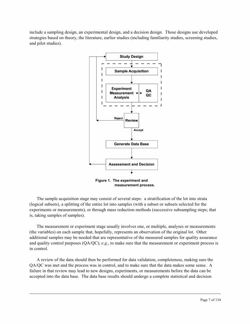
include a sampling design, an experimental design, and a decision design. Those designs use developed strategies based on theory, the literature, earlier studies (including familiarity studies, screening studies, and pilot studies).

Figure 1. The experiment and

measurement process.

The sample acquisition stage may consist of several steps: a stratification of the lot into strata (logical subsets), a splitting of the entire lot into samples (with a subset or subsets selected for the experiments or measurements), or through mass reduction methods (successive subsampling steps; that is, taking samples of samples).

The measurement or experiment stage usually involves one, or multiple, analyses or measurements (the variables) on each sample that, hopefully, represents an observation of the original lot. Other additional samples may be needed that are representative of the measured samples for quality assurance and quality control purposes (QA/QC); e.g., to make sure that the measurement or experiment process is in control.

A review of the data should then be performed for data validation, completeness, making sure the QA/QC was met and the process was in control, and to make sure that the data makes some sense. A failure in that review may lead to new designs, experiments, or measurements before the data can be accepted into the data base. The data base results should undergo a complete statistical and decision

Page 7 of 134

analysis before being accepted for the end use. The results of those analyses may generate a new study, again following the stages in Figure 1.

Our focus in this guidance document will be on developing a subsampling strategy for just one step in the sample acquisition stage of the measurement and experiment process (that is, the laboratory sample to the analytical subsample step); however, since our developing sampling strategy is bounded by our decision strategy, we will briefly discuss some of the decision aspects (such as the data quality objective (DQO) process, the bounds of what makes a representative sample, and some items to include in reporting the results). Although this focus is narrow, it behooves the analysts (unless they are involved in a “blind” study), and it certainly behooves the statisticians, scientists, managers, and decision makers, to consider the analytical subsample in the context of the entire measurement and experiment process.

1.7 Data Quality Objectives

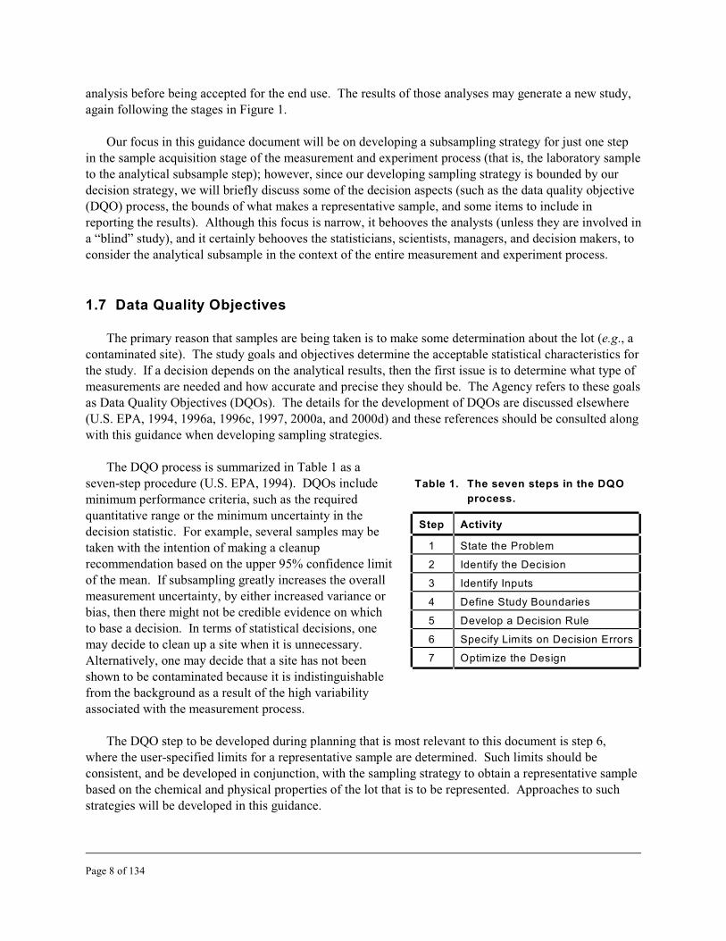
The primary reason that samples are being taken is to make some determination about the lot (e.g., a contaminated site). The study goals and objectives determine the acceptable statistical characteristics for the study. If a decision depends on the analytical results, then the first issue is to determine what type of measurements are needed and how accurate and precise they should be. The Agency refers to these goals as Data Quality Objectives (DQOs). The details for the development of DQOs are discussed elsewhere (U.S. EPA, 1994, 1996a, 1996c, 1997, 2000a, and 2000d) and these references should be consulted along with this guidance when developing sampling strategies.

The DQO process is summarized in Table 1 as a seven-step procedure (U.S. EPA, 1994). DQOs include Table 1. The seven steps in the DQO

minimum performance criteria, such as the required process.

quantitative range or the minimum uncertainty in the decision statistic. For example, several samples may be taken with the intention of making a cleanup recommendation based on the upper 95% confidence limit of the mean. If subsampling greatly increases the overall measurement uncertainty, by either increased variance or bias, then there might not be credible evidence on which to base a decision. In terms of statistical decisions, one may decide to clean up a site when it is unnecessary. Alternatively, one may decide that a site has not been

Step Activity

1 State the Problem

2 Identify the Decision

3 Identify Inputs

4 Define Study Boundaries

5 Develop a Decision Rule

6 Specify Lim its on Decision Errors

7 Optim ize the Design

shown to be contaminated because it is indistinguishable from the background as a result of the high variability associated with the measurement process.

The DQO step to be developed during planning that is most relevant to this document is step 6, where the user-specified limits for a representative sample are determined. Such limits should be consistent, and be developed in conjunction, with the sampling strategy to obtain a representative sample based on the chemical and physical properties of the lot that is to be represented. Approaches to such strategies will be developed in this guidance.

Page 8 of 134

1.8 Defining the Term, Sample, and Other Related Terms

Before too much confusion sets in, it may be prudent at this point to define the term, sample, and some other related terms that will be used frequently in this text. There is also a glossary at the end of the text that can be consulted for unfamiliar terms. The terminology used in this document will generally follow that of the Gy sampling theory (Pitard, 1993).

The Notion of Sample Size: Samples seem to come in all sizes and shapes and, depending on the context, one person’s definition of a sample may not be recognized by another person. There may be agreement that a statistical sample consists of a number of units from a target population. However, a simple question about sample size might be answered as 68 samples by someone concerned with the statistical aspects of a study, but as 50 g by the laboratory analyst. Due to this difference in terminology, anyone dealing with samples and sampling needs to be careful when summarizing the sampling process so that there is no misunderstanding.

The Notion of a Representative Sample: Strictly speaking, Pitard (1993) defines a correct sample as “a part of the lot obtained by the reunion of several increments and (which is) meant to represent the lot.” The key word to being acceptable as a sample is “representative.” As we will see later, there are degrees for being representative that are defined by the user, and a representative sample can only be ensured by using correct sampling practices. Thus, we should always use the qualifiers, nonrepresentative or representative, or incorrectly or correctly selected, when we use the terms, sample or subsample. Any material collected that is outside of the imposed limit of being representative should be qualified as nonrepresentative and anything collected that meets the user’s definition of being representative should be qualified as representative. Thus, we can have a nonrepresentative sample or a representative sample, and a nonrepresentative subsample or a representative subsample. More properly, a nonrepresentative sample (or subsample) or an “incorrectly” taken sample (or subsample) should be called a specimen and not a sample.

The Notions of a Lot and a Sampling Unit: A lot is the collective body of material under investigation to be represented; e.g., a batch, a population, or populations. A lot may consist of several discrete units (e.g., drums, canisters, bags, or residences), each called a sampling unit, or it may be an entire hazardous waste site. Since it is often too difficult to analyze an entire lot, a sample (a portion) is taken from the lot in order to make estimations about the characteristics of that lot. For example, sample statistics, such as the sample mean and sample variance, are used to estimate population parameters, such as the population mean and population variance. Because sampling is never perfect and because there is always some degree of heterogeneity in the lot, there is always a sampling error. To get accurate estimates of the lot by the sample(s) and to minimize the total sampling error, a “representative” sample is sought by using “correct sampling practices.”

The Notion of Correct Sampling (also known as Correct Selection): Unless correct sampling practices are used, the results from analyzing a subsample will usually be biased compared to the true value in the original sample. Correct sampling practices give each item (particle, fragment) of the lot an equal and constant probability of being selected from the lot to be part of the sample. Likewise, any item that is not considered to be part of the lot (that is, should not be represented by the sample) should have a zero probability of being selected. Any procedure that

Page 9 of 134

favors one part of the sample over another is incorrect. Correct sampling practices minimize the “controllable” errors by using correctly designed sampling devices, common sense, and by correctly taking many random increments combined to make the sample. To be truly representative, a correct sample must mimic (be representative of) the lot in every way, including the distribution of the individual items or members (particles, analytes, and other fragments or materials) of that lot. Thus, correct sampling should produce a subsample with the same physical and chemical constitution, and the same particle size distribution, as the parent sample. However, depending on predefined specifications, the sample may only have to be representative of only one (or more) characteristics of the lot, and estimated within acceptable bounds.

The Notions of a Subsample and Sampling Stages: Usually there is more than one sampling step or stage; that is, sampling can take place successively to obtain ever smaller masses from larger masses of material; i.e., taking samples of samples. The sampling process begins with the initial mass of the material to be represented, called the lot (also known as the population or a batch). A correct sample of the lot is a subset of the original mass collected using correct sampling practices with the intent of selecting a representative sample that mimics the lot in every way (or at least mimics the characteristics, chosen by the user, of the lot). Subsampling is simply a repetition of this selection process whereby the sample now becomes the new lot (since it is now the material to be represented) and is itself sampled. A subsample is simply a sample of a sample. We will generically use the term, subsample, as the smaller mass that is taken from the larger mass (which is called the sample) during the sampling (or, equivalently, the subsampling) step. We will also use the terms, parent sample and daughter sample, to describe this sample to subsample relationship, respectively. To literally describe all of the successive sampling steps in order from larger to smaller samples (or subsamples), the terms: lot (batch, site, or stratum), primary sample, secondary sample (or the subsample taken from the primary sample), tertiary sample (or the subsample taken from the secondary sample), and so on down to the end (or analytical) sample (or subsample) will be used. Assuming that the analytical error is relatively small and in control, and that correct sampling practices have been followed, the final analytical result can be termed a “representative measurement” (within user specifications) of the final analytical subsample. By extension, that measurement should be representative of each of the previous sampling stages right up to the original lot.

The Notion of a Perfect Sample: The perfect sample of a lot is one that is selected such that every individual object (particle, fragment, or other item) of that lot has an equal and independent probability of being included in the sample. Ideally, each object should be examined in turn, and selected or rejected based on a random draw with a fixed probability. In practice, the quality of any sampling tool or method is determined by how well the sample approximates the lot. Apart from the fundamental error due to (that is, “naturally” occurring from) the physical and chemical constitutional heterogeneity (differences) of the objects making up the lot, all of the sampling errors discussed in this document ultimately arise from the failure to select the lot’s objects with equal probability, or from the failure to select them independently.

The Notions of an Increment, a Composite Sample, and a Specimen: A few other terms that are related to, or sometimes confused with, the term, “sample,” should be mentioned. An “increment” is a segment, section, or small volume of material removed in a single operation of the sampling device from the lot or sample (that is, the material to be represented). Many

Page 10 of 134

increments taken randomly are combined to form the sample (or subsample). This process is distinct from creating a “composite sample,” which is formed by combining several distinct samples (or subsamples). A “specimen” is a portion of the lot taken without regard to correct sampling practices and therefore should never be used as a representative sample of the lot. A specimen is a nonprobabilistic sample; that is, each object (item, particle, or fragment) does not have an equal and constant probability of being selected from the lot to be part of the sample. Likewise, for a specimen, any object that is not considered to be part of the lot (that is, should not be represented by the sample) does not have a zero probability of being selected. A specimen is sometimes called a “purposive” or “judgement sample.” An example of a specimen is a “grab sample” or an “aliquot.”

The Notion of Sample Support: Another term, the sample “support,” affects the estimation of the lot (or population) parameters. The support is the size (mass or volume), shape, and orientation of the sampling unit or that portion of the lot that the sample is selected from. Factors associated with the support are the sample mass and the lot dimensionality.

The Notion of the Dimension of a Lot: If the components of a lot are related by location or time, then they are associated with a particular dimension. Lot dimensions can range from zero to four. Dimensions of one, two, or three, imply the number of long dimensions compared to significantly shorter dimensions. Bags of charcoal on a production line represent a one-dimensional lot. Surface contamination at a used transformer storage site is a two-dimensional lot. A railroad car full of soil contaminated with PCBs is a three-dimensional lot. However, determining the average level of PCBs in a train load of railroad cars deals with a zero-dimensional lot as long as the cars are considered a set of randomly ordered objects. Zero-dimensional lots are composed of randomly occurring objects (where the order of the units is unimportant), and this feature allows them to be characterized with the simplest experimental design. Four dimensions include time and the three spatial dimensions. The higher dimensional lots are more difficult to sample, but can often be transformed to have a smaller dimension.

Figure 2 shows one possible depiction of the sampling steps in the measurement process. The uncertainty in the estimate of the analyte concentration increases with every step in the process. A preliminary study of the sample matrix can be used to estimate the amount of sample necessary to achieve the study requirements. While this is not the primary goal of this document, it is directly related to the conceptual model supporting this guidance.

Page 11 of 134

Figure 2. A depiction of the sample acquisition process.

1.8.1 Heterogeneity

Much of this guidance deals with understanding and reducing the errors associated with heterogeneity. The reason that samples do not exactly mimic the lot that they are supposed to represent is because of the errors associated with heterogeneity. Heterogeneity is the condition of a population (or a lot) when all of the individual items are not identical with respect to the characteristic of interest. For this guidance, the focus is on the differences in the chemical and physical properties (which are responsible for the constitution heterogeneity, CH) of the particulate material and the distribution of the particles (which leads to the distribution heterogeneity, DH). Conversely, homogeneity is the condition of a population (or a lot) when all of the individual items are identical with respect to the characteristic of interest. Homogeneity is the lower bound of heterogeneity as the difference between the individual items of a population approach zero (which cannot be practically achieved).

Page 12 of 134

Thus, one can infer that, within predefined boundaries, heterogeneity is a matter of scale. That is, all materials exhibit heterogeneity at some level. With a very pure liquid, one might have to go to the molecular level before heterogeneous traits are identifiable; but, with particulate samples, heterogeneity is usually obvious on a macroscopic scale. This lack of uniformity is the primary reason for the added uncertainty when attempting to obtain a representative sample.

Since a sample cannot be completely identical to the lot (or parent sample), the next best goal is for it to be as similar to the lot (or parent sample) as possible. In terms of the particulate sample structure, this criterion is the same as requiring the physical or chemical constitution, and the distribution, of the particles to be as similar as possible for each type of particle in the sample as in the lot. Any process that increases heterogeneity will expand the differences, resulting in increased bias or increased variability, between the sample and the lot.

Representative particulate samples will have a finite mass, which means that there is a lower limit of the number of particles of any given form and type (physical or chemical characteristics). If the sample mass is too small, compared to the amount of material to be represented (the lot), then there may not be enough of the different types of particles in the sample to exactly mimic the lot, and the sample could have any one subset of numerous possible particle combinations. Any measured feature of the sample will be different depending on exactly which combination of particles ended up in the sample. The variability associated with selecting enough particles at random is the minimum uncertainty that will be present no matter how one takes a sample. The catch is knowing when enough particles are selected at random to be representative of the lot. A small sample mass (below this lower limit) can be achieved through a subsampling strategy involving comminution (for example, see the section on the sampling nomograph). The upper limit for the sample mass is obviously the entire lot mass.

Except for this natural fundamental error (FE) inherent to the particles being chemically or physically different, other contributions to heterogeneity can be minimized through “correct” sampling practices. Correct sampling (or selection) will be discussed in more detail later, but it can be associated with three practices: (1) taking many (N $30) increments to make up the subsample (to minimize the grouping and segregation error, GE), (2) using correctly designed sampling tools (to minimize the materialization error, ME), and (3) using common sense and vigilance (to minimize the preparation error, PE).

There are only two ways to reduce the effect of the relative variance of the fundamental 2heterogeneity (sFE ) associated with the physical and chemical constitution of particulate samples. One

way is by increasing the sample mass. If the sample mass is increased, the constitution of the different particles (and the distribution of the different particles) will more likely closely match the original particle distribution. A larger sample size also means that the relative influence of any given particle on the property of interest is smaller. The other way to reduce the uncertainty due to the heterogeneity of particle types is to decrease the influence of any given particle by breaking up the larger particles into several smaller particles (reducing the scale of heterogeneity). This crushing or grinding process is known as “comminution.” The smaller the particle size, the smaller the effect of including or excluding any type of particle in the sample. Comminution also has the advantage of liberating more contaminant that may be occluded in a larger particle, which could otherwise be masked from the analytical method. The result of either increasing the sample mass or reducing the particle size is a more likely representative estimate for the measured sample characteristic.

Page 13 of 134

For the purposes of environmental sampling, one can now deduce a quick rule-of-thumb: the sample should be fairly representative of the lot if the largest contaminated particles of the sample are representative of the largest contaminated particles of the lot. Remember that it is the physical and chemical constitution of the particles that leads to the constitution heterogeneity and the fundamental variability, and the greatest fundamental variability (sFE

2) associated with contamination should be the largest contaminated particles (we will see later that this contribution to variability will show up as the

3cube of the diameter of the largest contaminated particles, d , in the equation describing the relative variance of the fundamental error, sFE

2).

1.8.2 Laboratory Subsampling: The Need for Sample Mass Reduction

There are several reasons for laboratory sample mass reduction. The most common reason is to select the amount of sample required in an analytical protocol. Field samples are generally much larger than needed for laboratory analysis. Low mass requirements for analytical methods are driven by improved technology and by the cost savings associated with ever smaller amounts of reagents, equipment, and waste per sample run. For example, a chemical extraction might call for 2 g of material. However, if the original sample amount is 164 g, it is not immediately obvious how one should process the sample to obtain a 2 g subsample that is representative of that entire 164 g sample. Another reason for subsampling may be to generate quality control information, such as some replicate analyses using the same or an alternate analysis method. The study design may also call for a separate determination of the concentration of other analytes or additional physical or chemical properties of the sample, each requiring a separate subsample. If decisions are to be made with respect to a bulk property, then the subsample should accurately and precisely represent that property. This problem of selecting a representative sample has been extensively studied in the mineral extraction industries, culminating with Pierre Gy’s theory of sampling particulate material (Gy, 1982, 1998; Pitard, 1993; and Smith, 2001). Though there are several alternative approaches to this problem (Visman, 1969; Ingamells and Switzer, 1973; and Ingamells, 1976), it has been shown that each type of theoretical approach is similar to Gy sampling theory (Ingamells and Pitard, 1986). Before a representative sample is defined and a strategy to obtain a representative sample is developed, an understanding of some of the salient points of the Gy sampling theory would be beneficial.

Page 14 of 134

Section 2

Overview of Gy Sampling Theory

The uncertainty associated with sampling is a product of both the sample (physical and chemical attributes) and the sampling process (involving statistical issues and sampling technique). These topics are discussed in the context of the Gy sampling theory as applied to environmental samples. The sampling theory of Pierre Gy has been applied very effectively in the mining industry since he introduced it in 1953; however, very little experimental verification has been attempted and even less research has been demonstrated for environmental samples. We are focusing on Gy theory because we believe that it is the state-of-the-science sampling theory that identifies and minimizes the errors associated with sampling particulate materials, and we have done experiments to verify and demonstrate the effectiveness of Gy theory. This theory not only covers the statistical issues of sampling particulate materials, but also blends in the effects of the physical and chemical attributes of the particulate material! Gy theory introduces the notion of “correct” sampling to obtain a representative subsample. The relevant components of Gy sampling theory are discussed and factors that are indicative of large errors are identified. Specific examples are provided to highlight the conditions that may result in highly uncertain results caused by incorrect sampling practices.

2.1 Background

Sampling theories have been developed in an effort to move toward sampling methods that reduce or minimize the uncertainty from the sampling component of the measurement process. Gy sampling theory is a comprehensive approach to understanding and assessing all of the sources of uncertainty affecting the estimation of a target analyte concentration (Pitard, 1993; and Smith, 2001). While a comprehensive discussion of Gy sampling theory is beyond the scope of this document, an abbreviated introduction to the principal concepts and terminology is provided throughout this document.

Historically, Gy's methods for sampling heterogeneous particulate solids were developed in the mid­1950s for the mining industry to sample crushed ore. The ore is thought of as consisting of an inert substance (gangue) and a valuable material (gold or some other metal or metals), which are intimately intermixed. Even though the ore is crushed to some degree of fineness, some of the “value” is hidden from the assay by a covering or armor of the gangue. The smaller the diameter of the particles, the more the “value” is released to be measured in the assay.

The Gy sampling theory is generally applicable to matrices of particulate solids, with the analytes of interest (contaminants) presumably being no more volatile than organic semi-volatile compounds. Nonetheless, the application of Gy theory to environmental samples, especially containing semi-volatile and volatile compounds, needs to be further researched.

Page 15 of 134

2.2 Uncertainty Mechanisms

If a study generates data with very large errors, then the uncertainty in the results may prevent one from making a sound scientific conclusion. There are many possible sources of uncertainty to consider when processing or analyzing a sample, and the study designs or an analyst’s expertise is relied upon to identify and avoid as many of those sources of error as possible. Many of those error mechanisms can occur when obtaining any types of samples, including particulate material samples. While it is important to address all of the factors (such as analytical errors, AE) that might produce an incorrect value, the following discussion is limited to the uncertainty mechanisms related to selecting a particulate subsample. As will be seen, the uncertainty associated with discrete particles may be much larger than expected. In order to identify an appropriate sampling method, one must first understand the different types of errors that can arise from particulate samples. The rest of this section discusses the types of errors related to sampling particulate materials.

2.3 Gy Sampling Theory: Some Assumptions and Limitations

Before trying to apply Gy sampling theory, one must first verify that the sample matrix meets certain assumptions, otherwise some alternative sample splitting guidance should be followed. Gy sampling theory is applicable to samples composed of particulate material, with most applications related to extractable compounds existing as high concentration mineral grains or inclusions produced by anthropomorphic or geochemical processes. Particle types are usually presented as if there is a discrete set of compositions or structures rather than a continuous range. Environmental hazardous materials often coat natural materials, are absorbed into the particle, or exist as separate particles. Those cases are all accommodated by Gy sampling theory; however, the application of the Gy sampling theory to environmental hazardous materials is in its infancy and examples are rare in the literature. Such cases warrant more research.

Some sample types appear to be described by Gy sampling theory, but closer scrutiny reveals that they fail to meet one or more assumptions. For example, PCBs in sediments occupy the interstitial spaces between the particle and are absorbed into the particles. If the PCBs are fully integrated into the particles, then Gy sampling theory can be applied, otherwise it may be inappropriate. Similarly, suppose the sample was a mixture of sand and gravel from a beach. If the contaminant was crude oil, Gy sampling theory may not fully apply, as the analyte was not a solid and is present as an interstitial fluid. Again, this is an area for future sampling research.

Gy sampling theory assumes a mathematical model for the analyte level across the entire range of possible samples, and that model is that the analyte concentration varies about a mean. With this model, the primary goal is to estimate the mean value, and any difference from the mean is considered an error. Suppose a Superfund site is contaminated very highly in the center and the contaminant levels drop as one moves outward. If the entire site is to be represented, then Gy sampling theory would imply that there is a high (positive) error at the center, a high (negative) error near the edges, and a low error in a circular zone about the center (see Figure 3). Only samples near the circular zone would have analyte levels near the average for the site. Of course, samples would not be taken from just one (or even a few) location, and many random increments would be taken to make up each sample to represent the lot.

Page 16 of 134

Nonetheless, one must be careful in the interpretation and the application of Gy sampling theory in environmental characterizations. If it is important that the average for the entire lot (site) is known, then the application of Gy theory for the entire lot is appropriate. Otherwise, it may be more informative to strategically divide (stratify) the lot into several smaller lots (strata) and find the average concentration for each smaller lot (stratum). The strategies employed for such stratification are covered in the field of geostatistics using screening strategies and tools like semi-variograms. Such topics will be discussed in the (planned) future field subsampling guidance. However, the sampling theory for large lots is generally applicable for smaller lots, such as laboratory samples.

Figure 3. Contour plot of contaminant level across a hazardous waste site.

2.4 Gy Sampling Theory: Errors

Gy sampling theory identifies the distinct activities of the sampling process and partitions the error between them. Of the seven basic sampling errors identified by Gy sampling theory (see Table 2), only five of those errors will be considered and are relevant to preparing laboratory subsamples from particulate samples. The long-range heterogeneity fluctuation error (CE ) and the periodic heterogeneity 2

fluctuation error (CE ) will not be considered here and are presumed to be negligible or inconsequential 3

for preparing laboratory subsamples from relatively small (in mass) particulate samples. However, those errors should be considered for larger samples (e.g., drums and large field samples) or larger lots (sites or strata from sites). Those errors will be considered and discussed in a planned guidance for obtaining representative field samples.

Page 17 of 134

Table 2. Gy sampling theory error types for particulate materials.

Notation Error Type Subject / Description

1. FE Fundamental Error A result of the constitutional heterogeneity, CH (the

particles being chemically or physically different).

2. GE Grouping and Segregation

Error

A result of the distributional heterogeneity, DH.

3. 2CE Long-Range Heterogeneity

Fluctuation Error

Trends across space or over time.

4. 3CE Periodic Heterogeneity

Fluctuation Error

Periodic levels across space or over time.

5. DE Increment Delimitation Error Identifying the correct sample to take. Considers

the volume boundaries of a correct sampling device.

6. EE Increment Extraction Error Removing the intended sample. Considers the

shape of the sampling device cutting edges.

7. PE Preparation Error Sample degradation, gross errors, analyte loss or

gain.

Note that these Gy errors are relative variance (squared relative deviation) errors and are with respect to the simple model that all of the sample results are supposed to be at the mean value for the lot. Any deviation from the model is considered an error. The five remaining Gy sampling error types play an important role in determining the uncertainty levels for particulate samples and will be discussed in more detail below.

2.5 Subsample Selection Issues

Little attention is usually paid to the actual selection of a subsample. However, in many circumstances, a highly biased value will result if sampling procedures are not appropriately matched to the sample matrix. The variability associated with subsampling depends on several physical and chemical characteristics, including:

• particle shapes

• particle sizes

• number of particles

• number of particle types

• particle mass (or density)

• particle chemical composition

• analyte chemical composition

•other gangue (matrix) chemical and physical composition (moisture content, liquids, amorphous solids, or other occluded or interstitial materials)

• analyte concentrations in each particle type

• particle size distribution

Page 18 of 134

These characteristics primarily affect the fundamental error, which is associated with the constitution (or composition) heterogeneity (chemical and physical differences between the particles), and with the grouping and segregation error, which is associated with the distribution heterogeneity (due largely to gravitational effects across the sample). The random distribution of the particles will result in some degree of heterogeneity of the target analyte even if the sample is free from additional heterogeneity effects such as gravitational fractionation. The sample mass required to meet the study requirements will depend on all of the above characteristics and will also be a function of the desired level of accuracy and precision required by the study.

The correct selection of the subsample also depends on the sample support, the dimensionality of the lot, and the design of the sampling tool or device – all of which affect the materialization error.

Common sense used in the selection process is the key to reducing the preparation error.

2.6 The Relationship Between the Gy Sampling Theory Errors

To correctly apply Gy sampling theory, one needs to understand the nature and source of all of the components of sample variation. If the magnitude of each error component can be determined, then the dominant error sources can be identified and one can avoid efforts that would have no substantial impact on the variability.

The overall estimation error (OE) is the difference between the final analytical estimate of the characteristic of interest (such as an estimation of the average concentration of an analyte in the lot based on sample analysis) and the true (usually unknown) value of that characteristic of interest (such as the true average concentration of that analyte in the lot). The overall estimation error would be the error associated with the final value given in the measurement and experiment process. Pitard (1993) gives this as the sum of the total sampling error (TE) and the analytical error (AE). That is,

OE = TE + AE

The analytical error (AE) includes all of the uncertainty and errors introduced during the laboratory phase of a study. The analytical error is the cumulative error associated with each stage of the analytical method, such as chemical extraction, physical concentration, electronic detection, uncertainty in the standards, fluctuations due to temperature variations, etc. Care should be taken when reviewing claims about analytical error. Occasionally these claims refer only to one component of the analytical procedure, such as the stability of the measurement apparatus. Instrumental errors are typically quite small compared to the error associated with characterizing the sample. The analytical error is not a sampling error and is the subject of fields such as analytical chemistry and experimental design and will not be discussed here in any detail. It should be noted that the variability added by the sampling process can easily exceed the uncertainty associated with analytical chemistry methods (Jenkins et al., 1997). The total sampling error is the subject for discussion in this text.

Page 19 of 134

When Gy sampling theory is presented in the context of determining the level of an analyte (or a pollutant) in a lot, error usually refers to any deviation from the mean. The total sampling error (TE) can be defined as

where a is the actual (mean) content of the analyte in the lot and a is a measure of the (mean) L s

content of the analyte in the sample (it is the sample estimator of aL). The conceptual additive linear model given by Gy for the total sampling error is:

where SE is the sampling or selection error, PE is the preparation error, and n is the index for the sampling stage. The total sampling (or selection) error, TE, for one stage is then:

TE = SE + PE

The selection error (SE) is a linear combination of the continuous selection error, CE, and the materialization error, ME, and is given as

SE = CE + ME

The continuous selection error, CE, is a linear combination of the short-range heterogeneity fluctuation error, CE , the long-range heterogeneity fluctuation error CE , and the periodic 1 2

heterogeneity fluctuation error, CE , and is given by 3

CE = CE1 + CE + CE2 3

The short-range heterogeneity fluctuation error, CE , is given by a linear combination of the 1

fundamental error, FE, and the grouping and segregation error, GE

CE1 = FE + GE

The increment materialization error is given by a linear combination of the delimitation error (DE) and the extraction error (EE)

ME = DE + EE

The total sampling error is then

TE = FE + GE + CE + CE + DE + EE + PE 2 3

If correct sampling practices are used, then the terms, GE, DE, EE, and PE are minimized; that is, GE + DE + EE + PE . 0. Assuming that CE + CE = 0 (that is, they are negligible for 2 3

Page 20 of 134

laboratory subsampling), and if correct sampling practices are used, then the total sampling error becomes

This is the minimum sampling error due simply to the nature of the material being sampled (the constitution heterogeneity) and represents a goal of Gy’s correct sampling practices.

Likewise, the additive relative variances linear model given by Gy for the relative variance of the total sampling error is

2sTE2 = s SE

2 + sPE

2 2where sSE is the relative variance of the sampling or selection error and s is the relative PE

variance of the preparation error. The relative variance of the selection error is given as

2sSE2 = sCE

2 + sME

Since the relative variance of the continuous selection error is given by

2 2sCE2 = sCE1 + sCE2 + sCE3

2

and the relative variance of the short-range heterogeneity fluctuation error is given by a linear combination of the relative variance of the fundamental error and the relative variance of the grouping and segregation error

2sCE12 = sFE

2 + sGE

and the relative variance of the increment materialization error is given by a linear combination of the relative variance of the increment delimitation error and the relative variance of the increment extraction error

2sM E2 = sDE

2 + sEE

then the relative variance of the total sampling error is

2 2 2sTE2 = sFE

2 + sGE + sCE22 + sCE3 + sDE

2 + sEE + sPE2.

2 2 2 2If correct sampling practices are used, then the terms, sGE , sDE , s , and s are minimized; thatEE PE 2 2 2 2is, s + sDE

2 + sEE + sPE2 . 0. Assuming that sCE2 + sCE3 = 0 (that is, they are negligible for GE

laboratory subsampling), and if correct sampling practices are used, then the relative variance of the total sampling error becomes

2s = sFE2

TE

This is the minimum sampling relative variance due simply to the nature of the material being sampled (the constitution heterogeneity) and is the basis for developing a representative sampling strategy using Gy’s correct sampling practices.

Page 21 of 134

The mean of the total sampling error is

The mean of the fundamental error (under the above conditions of correct sampling practices and negligible effects from CE and CE3) is expected to be negligible; that is, 2

The relative variance of the total sampling error is given by

And, under the above conditions of correct sampling practices and negligible effects from sCE2

and sCE32, the relative variance of the fundamental error is

Thus, the greater the variation is in the physical and chemical characteristics between each of the particles (or other materials) in the lot, the greater the variance is in the constitution heterogeneity and, consequently, the larger will be the relative variance of the fundamental error,

2s .FE

2.7 The Short-Range Heterogeneity Fluctuation Error, CE1

All particulate samples are heterogeneous; it is just a matter of scale. How closely one particle resembles another particle is dependent upon the focus of the sampler. One common feature of heterogenous particulate material is that it consists of a distribution of particles (and perhaps other materials, such as oils) with diverse physical and chemical characteristics, including different: particle sizes, particle shapes, textures, concentrations of various chemical constituents, and densities. The differences in the chemical and physical properties of the constituents of the lot are responsible for the constitution heterogeneity (sometimes called the composition heterogeneity), CH. The constitution heterogeneity is the source of an expected minimum error, the fundamental error (FE). If there are groups of items (particles, fragments, or other objects) in the lot that do not have the same average composition, then there is a distribution heterogeneity, which is often caused by gravity. It is the distribution heterogeneity, DH, that leads to the grouping and segregation error, GE.

Page 22 of 134

2

The short-range heterogeneity fluctuation error is a linear combination of those two errors and is given by

CE1 = FE + GE

2.8 The Fundamental Error (FE) - the Heterogeneity of Particulate

Constitution

This error is fundamental to the composition of the particles, being chemically or physically different and is a result of the constitution heterogeneity (CH) (see Figure 4). It is the minimum sampling error and the expected error if the sampling operation is perfect. It is also the only error that can be estimated before the sampling operation. The fundamental error is the error expected if the individual particles for a sample are selected at random from the particles making up the lot. The fundamental error is only a result of the chemical and physical constitution heterogeneity of the material, and not the sampling process. The fundamental error is usually dominated by particle size and composition properties. While sampling activities can add additional error, the sampling process cannot reduce the fundamental error. The bias of the fundamental error is expected to be negligible for most cases (Pitard, 1993; p. 167) and the relative variance of the fundamental error may be reduced by decreasing the diameter of the largest particles of the matrix to be represented, or by increasing the mass of the sample, Ms [g].

Figure 4. A depiction of the fundamental error (FE) due to the composition of the particles (or other items

or fractions) of the lot being chemically or physically different. It is a result of the constitution

heterogeneity (CH) of the lot; thus, this is the only sampling error that can never cancel out.

The fundamental error (FE) is the error of the measured subsample property that is expected if the particles in the subsample were selected one at a time from the sample at random (that is, each random increment making up the sample is a single particle. Of course, this is not a practical way to sample!). Any subsampling method will result in a subsample that has a slightly different property than the original sample. The variability in results that is independent of the subsampling process will depend on the variability associated with the individual particles. One can consider the effect of including or excluding an individual particle and asking what the relative effect will be. If all of the particles are small, then there will be a small change associated with adding or removing one particle. If some particles are large (or highly concentrated), then there may be a larger change associated with the inclusion or exclusion of a single particle.

Page 23 of 134

The fundamental error is unaffected by whatever sample selection practice is used. It is always present. Any sample selection practice that provides a less random selection of particles will result in a larger uncertainty. One cannot stress too highly that a minimum error level is expected that depends only on the physical and chemical constitution of the particles in the sample. The fundamental error is unrelated to the selection method used in generating a subsample.

As mentioned above, there are only two ways to decrease the relative variance of the fundamental error. One way is to change the sample mass, M . If the sample mass is doubled, then the uncertainty in s

results will be lower (if sampling is done “correctly”). This makes common sense – the more mass of the lot that is sampled, the more the sample becomes like the lot. Taking a larger sample has the same type of effect on the magnitude of the relative variance of the fundamental error as one gets by analyzing multiple samples to reduce the uncertainty in estimating the mean. How large the sample needs to be in order to achieve the study goals depends on how large the relative variance of the fundamental error is compared to the maximum allowed error for the study. If the sample contains large particles, then one may need a relatively large sample to meet the study uncertainty requirements. Often the size of sample needed to achieve the DQOs can be too large for a standard laboratory to process. The other method for changing the effect of the fundamental error is to alter the nature of the sample by crushing or grinding (the process of comminution) it to reduce the maximum particle size. A smaller particle size will lower the relative variance of the fundamental error for a fixed subsample mass.

There are a number of other factors that can increase the sampling variance beyond the fundamental error. Minimizing sampling variability without particle size reduction can be accomplished through the careful selection of all phases of the subsampling process. Whether or not this is cost-effective depends on the relative size of the different error components (see Table 2) and the sample mass needed to achieve success. However, minimizing those other error components has no effect on the fundamental error. If the relative variance of the fundamental error is too large, the results will not be conclusive no matter how carefully the rest of the sampling and analysis procedures are performed!

Because our strategy to obtain a representative sample relies on correct sampling methods to minimize all of the “controllable” errors, we will first discuss those controllable errors and then focus in on the fundamental error (specifically sFE

2) with more details in the section appropriately entitled, “Fundamental Error Fundamentals.”

2.9 The Grouping and Segregation Error (GE) – the Heterogeneity of

Particle Distributions

Another source of uncertainty is related to the particle distribution and the distribution of the analyte throughout the sample. This error is due to the non-random short range spatial distribution of the particles and the analyte due to grouping and segregation (usually because of gravity); i.e., incremental samples are different (see Figure 5). This grouping and segregation error (GE) is a result of the variability due to the heterogeneous distribution of the particles, known as the distribution heterogeneity (DH). This error may be minimized by combining many random increments, taken correctly from the lot to be represented, to form the sample.

Page 24 of 134

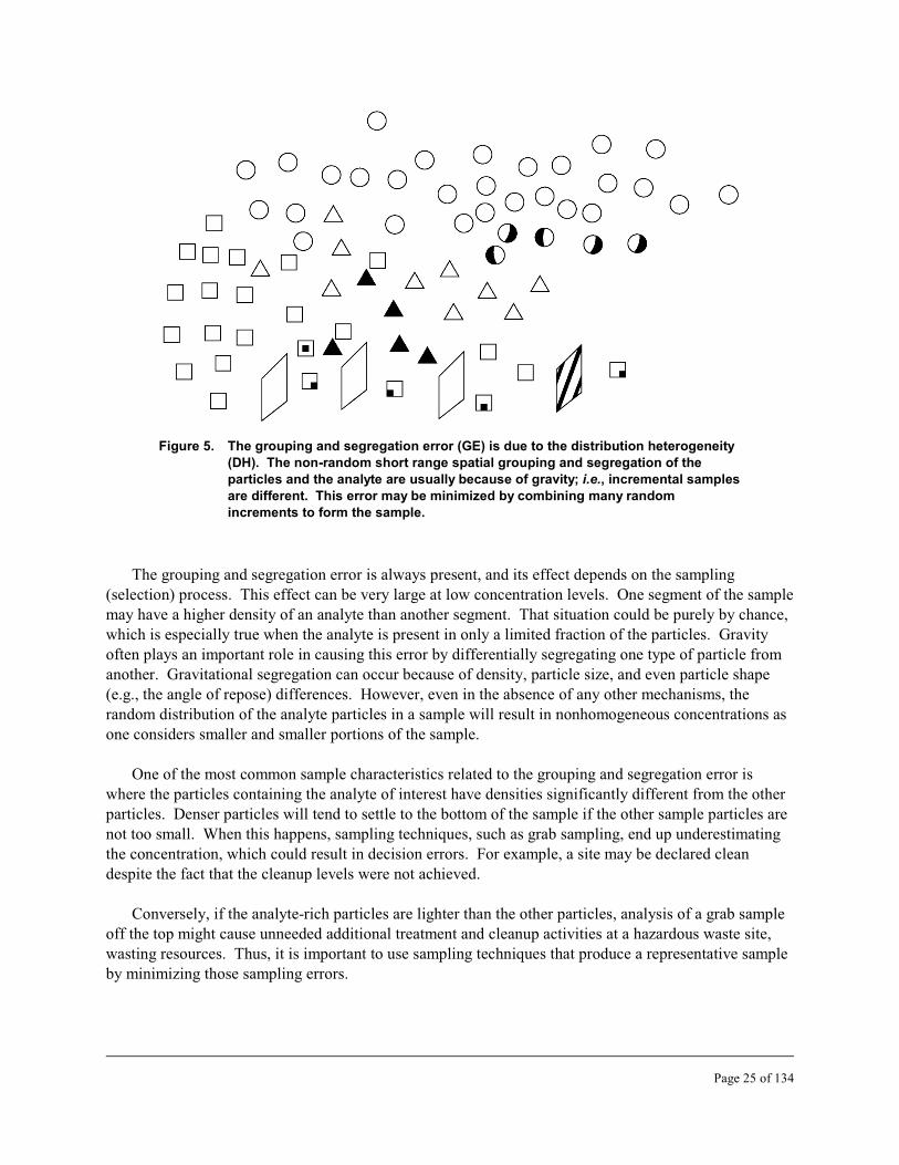
Figure 5. The grouping and segregation error (GE) is due to the distribution heterogeneity

(DH). The non-random short range spatial grouping and segregation of the

particles and the analyte are usually because of gravity; i.e., incremental samples

are different. This error may be minimized by combining many random

increments to form the sample.

The grouping and segregation error is always present, and its effect depends on the sampling (selection) process. This effect can be very large at low concentration levels. One segment of the sample may have a higher density of an analyte than another segment. That situation could be purely by chance, which is especially true when the analyte is present in only a limited fraction of the particles. Gravity often plays an important role in causing this error by differentially segregating one type of particle from another. Gravitational segregation can occur because of density, particle size, and even particle shape (e.g., the angle of repose) differences. However, even in the absence of any other mechanisms, the random distribution of the analyte particles in a sample will result in nonhomogeneous concentrations as one considers smaller and smaller portions of the sample.

One of the most common sample characteristics related to the grouping and segregation error is where the particles containing the analyte of interest have densities significantly different from the other particles. Denser particles will tend to settle to the bottom of the sample if the other sample particles are not too small. When this happens, sampling techniques, such as grab sampling, end up underestimating the concentration, which could result in decision errors. For example, a site may be declared clean despite the fact that the cleanup levels were not achieved.

Conversely, if the analyte-rich particles are lighter than the other particles, analysis of a grab sample off the top might cause unneeded additional treatment and cleanup activities at a hazardous waste site, wasting resources. Thus, it is important to use sampling techniques that produce a representative sample by minimizing those sampling errors.

Page 25 of 134

The fewer the number of analyte particles, the higher will be the relative variance of the short-range 2 2heterogeneity fluctuation error (that is, due to s or sGE ) expected from sampling. High analyte FE

concentration levels associated with those particles also cause an increase in variance. This is easily seen in Figure 6 (Pitard, 1993, p. 368) which shows a two-dimensional lot with a small number of high-level concentration analyte particles. The rate at which contaminant particles are found is expected to be very low. Analytical results from the samples can be approximated by a normal distribution if those samples contain more than a few analyte particles. As the sample mass decreases or the number of analyte

Figure 6. The effect of sample size when there are few analyte particles (black dots) (Pitard, 1993; p. 368).

particles drops to fewer than 5 to 7 per sample, the variability of the analyte in the samples will change. Instead of a Gaussian distribution, the data will then follow a Poisson distribution when plotted as the probability that a discrete number of analyte particles, P(r), will appear in a sample versus that number of analyte partilces, r, in a sample. Note that the Poisson distribution becomes more symmetrical, like a Gaussian distribution, as the number of analyte particles per sample increases above 4 (Pitard, 1993; pp. 357 ff.).

The expected effects from taking a smaller sample are reported by Starr et al. (1995), who notes, “The smaller diameter samples gave smaller means, greater skewness, and higher variances . . . .” A smaller sample mean is expected if there is less chance that a high analyte concentration level particle will be included in the sample, reducing the reported average concentration unless exhaustive analysis is performed. When a high-level analyte particle is present in a sample, the smaller the size of that sample, the larger will be the concentration estimate for that sample. And that will result in a higher estimate for the variance. A lot with a low number of analyte particles is a difficult case to deal with. Often the most difficult part in properly sampling this type of lot is to identify whether or not the sample falls into this category in the first place.

Page 26 of 134

Many analysts rely on mixing (or blending) as a preliminary “homogenization” step before taking a grab sample. Unfortunately, many samples cannot be made homogeneous enough for sampling by mixing, and such a procedure should not be relied upon to reduce GE. Segregation of particles by gravitational effects usually occurs at the moment that the mixing has stopped. Some samples will remain segregated even during the mixing process. Even if the mixing was effective, the subsampling step will still involve the same minimum error contributions from the fundamental error and the grouping error due to the random placement of analyte particles within the sample. The incorrect nature of grab sampling exacerbates the uncertainty by maximizing the error components from grouping, segregation, delimitation, and extraction processes. Grab sampling has been shown to be an unacceptable sampling method and should not be used with particulate samples (Allen & Khan, 1970; and Gerlach et al., 2002).

The relative variance due to the grouping and segregation error, sGE2, can be made relatively small

compared to the relative variance due to the fundamental error, sFE2, by increasing the number of random

2 2increments, N. For most cases, one can assume (Pitard, 1993; p. 189) that sGE # sFE ; therefore, since 2sCE1

2 = sFE2 + sGE ,

2 2sCE12 = sFE

2 + sGE # 2 sFE .

(Note that this is not always true; for example, a sample made of only one increment containing a highly 2 2segregated fine material may have a very small s but a much larger s ). Then, for N increments, FE GE

taken with correct sampling practices, we can write (Pitard, 1993, p. 388)

sGE2 . sFE

2 / N

and, under such conditions, the relative variance of the total sampling error becomes

2 2 2sTE2 $ sCE1 # sFE + [s / N]. FE

2 2Thus, one can see that sTE $ sCE12 . sFE if N is made large enough. At least N = 30 increments are

2 2recommended as a rule of thumb to reduce sGE compared to s (Pitard, 1993; p. 187). If this is too FE 2difficult in practice, then try to get at least 10 randomly selected increments. The goal is to reduce s GE

relative to sFE2 and you more or less “get what you pay for” in terms of this effort.

2.10 The Long-Range Heterogeneity Fluctuation Error (CE )2

The long-range heterogeneity fluctuation error refers to non-random, non-periodic trends across one or more dimensions of the lot and is commonly identified by variographic experiments. This error term will not be considered for laboratory subsampling. In environmental studies, identifying this type of heterogeneity is usually considered an objective of the sampling program, such as mapping concentration trends across a site such as one sees in Figure 3. The error is inherent to the distribution of analyte across a site and cannot be reduced by taking additional samples. CE is the regionalization term used in 2

geostatitics; that is, it is the region of autocorrelation between the nugget effect, V , and the sill of the o

semi-variogram. Taking additional samples helps to characterize this type of spatial heterogeneity instead of reducing it.

Page 27 of 134

2.11 The Periodic Heterogeneity Fluctuation Error (CE )3

This error is identified by variographic experiments and may be “smoothed out” by reducing the size of the strata or taking many increments to form the sample. The periodic heterogeneity fluctuation error is a (typically) long-range error with a repeating intensity pattern. An example of this type of error may be found when sampling soils over time and analyzing for nitrogen. One might find periodic fluctuations in the nitrogen levels through several years of data related to seasonal growth and decay patterns. As with the long-range heterogeneity fluctuation error, such information is more likely be the object of a study rather than in determining the mean analyte level. Again, this error is usually not a concern for laboratory subsampling.

2.12 The Increment Materialization Error (ME), the Increment Delimitation

Error (DE) and the Increment Extraction Error (EE): Subsampling Tool

Design and Execution

The increment materialization error (ME). Another potentially overwhelming, but often overlooked, source of uncertainty from sampling is from the variability added during the actual physical process of selection – that is, how to correctly select, prepare, and form the increments that are combined to make the sample (or subsample) using correctly designed sampling tools. The error associated with the execution of the increment selection and sample preparation process is called the increment materialization error (ME) and is technically the sum of three errors: (1) the increment delimitation error (DE), (2) the increment extraction error (EE), and (3) the preparation error (PE). That is, technically, ME = DE + EE + PE. However, only the increment delimitation error and the increment extraction error are associated with the increment selection process. Therefore, we will follow Pitard’s suggestion (Pitard, 1993) and separate out the preparation error from the materialization error; that is, we will use ME = DE + EE. Those two errors will be discussed in this section. The preparation error results from a nonselective process and will be discussed in a separate section.

The increment delimitation error (DE). Each sampling protocol describes a process by which the subsample is taken. If the protocol does not follow correct sampling practices, there may be a delimitation error. The delimitation error arises when the sampling process does not give an equal probability of selection for all parts of the sample. An error will be introduced if the sampling device selects or includes particles from any part of the lot with unequal probability.

Page 28 of 134

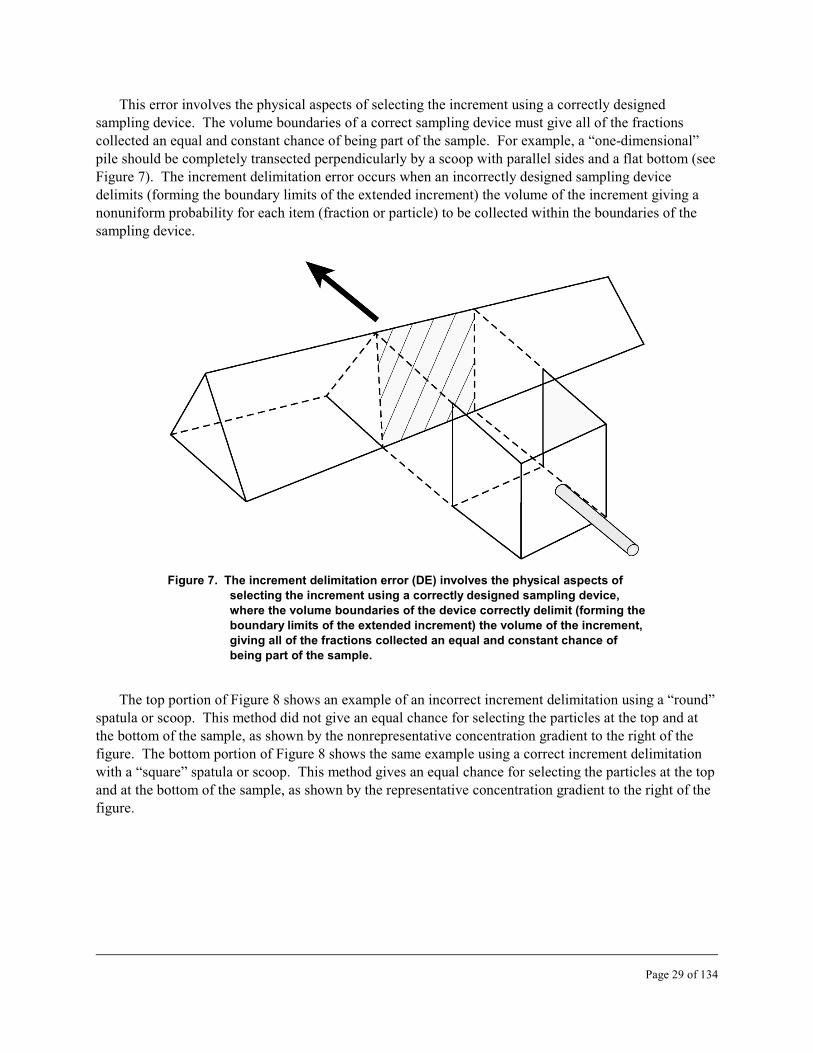
This error involves the physical aspects of selecting the increment using a correctly designed sampling device. The volume boundaries of a correct sampling device must give all of the fractions collected an equal and constant chance of being part of the sample. For example, a “one-dimensional” pile should be completely transected perpendicularly by a scoop with parallel sides and a flat bottom (see Figure 7). The increment delimitation error occurs when an incorrectly designed sampling device delimits (forming the boundary limits of the extended increment) the volume of the increment giving a nonuniform probability for each item (fraction or particle) to be collected within the boundaries of the sampling device.

Figure 7. The increment delimitation error (DE) involves the physical aspects of

selecting the increment using a correctly designed sampling device,

where the volume boundaries of the device correctly delimit (forming the

boundary limits of the extended increment) the volume of the increment,

giving all of the fractions collected an equal and constant chance of

being part of the sample.

The top portion of Figure 8 shows an example of an incorrect increment delimitation using a “round” spatula or scoop. This method did not give an equal chance for selecting the particles at the top and at the bottom of the sample, as shown by the nonrepresentative concentration gradient to the right of the figure. The bottom portion of Figure 8 shows the same example using a correct increment delimitation with a “square” spatula or scoop. This method gives an equal chance for selecting the particles at the top and at the bottom of the sample, as shown by the representative concentration gradient to the right of the figure.

Page 29 of 134

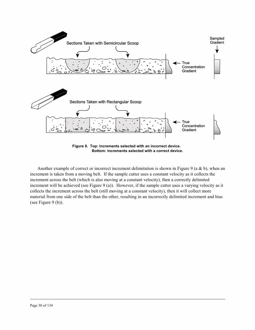
Figure 8. Top: increments selected with an incorrect device.

Bottom: increments selected with a correct device.

Another example of correct or incorrect increment delimitation is shown in Figure 9 (a & b), when an increment is taken from a moving belt. If the sample cutter uses a constant velocity as it collects the increment across the belt (which is also moving at a constant velocity), then a correctly delimited increment will be achieved (see Figure 9 (a)). However, if the sample cutter uses a varying velocity as it collects the increment across the belt (still moving at a constant velocity), then it will collect more material from one side of the belt than the other, resulting in an incorrectly delimited increment and bias (see Figure 9 (b)).

Page 30 of 134

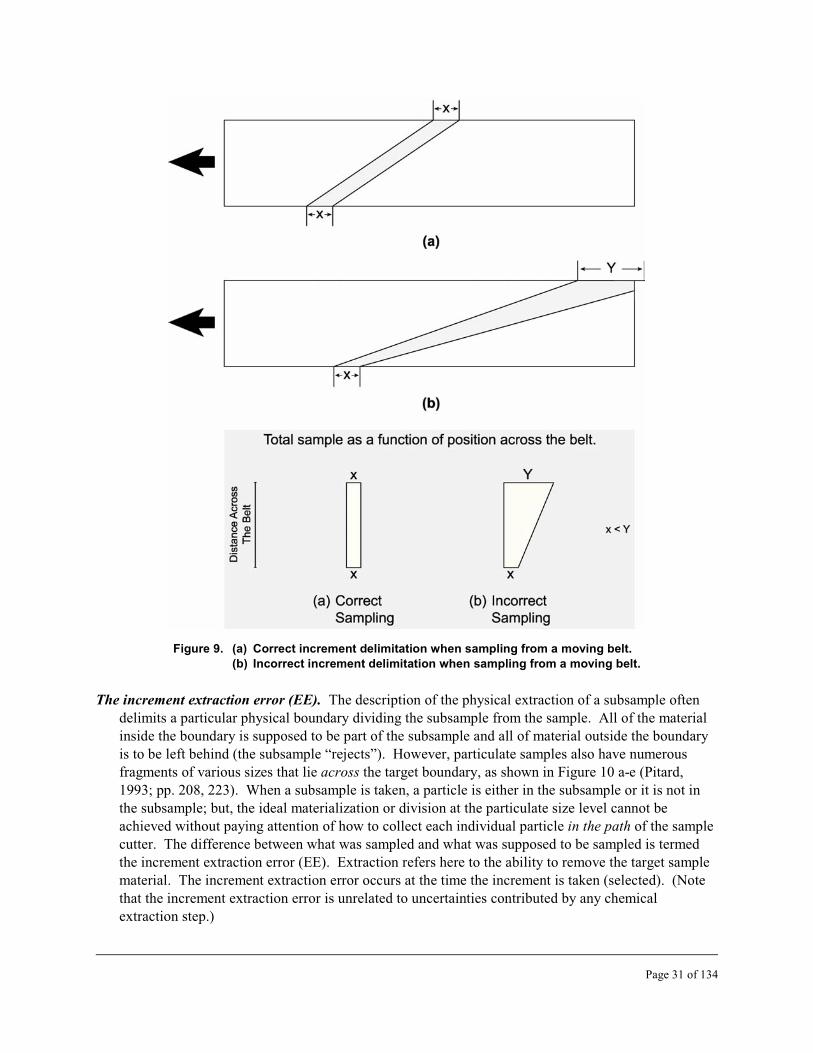
Figure 9. (a) Correct increment delimitation when sampling from a moving belt.

(b) Incorrect increment delimitation when sampling from a moving belt.

The increment extraction error (EE). The description of the physical extraction of a subsample often delimits a particular physical boundary dividing the subsample from the sample. All of the material inside the boundary is supposed to be part of the subsample and all of material outside the boundary is to be left behind (the subsample “rejects”). However, particulate samples also have numerous fragments of various sizes that lie across the target boundary, as shown in Figure 10 a-e (Pitard, 1993; pp. 208, 223). When a subsample is taken, a particle is either in the subsample or it is not in the subsample; but, the ideal materialization or division at the particulate size level cannot be achieved without paying attention of how to collect each individual particle in the path of the sample cutter. The difference between what was sampled and what was supposed to be sampled is termed the increment extraction error (EE). Extraction refers here to the ability to remove the target sample material. The increment extraction error occurs at the time the increment is taken (selected). (Note that the increment extraction error is unrelated to uncertainties contributed by any chemical extraction step.)

Page 31 of 134

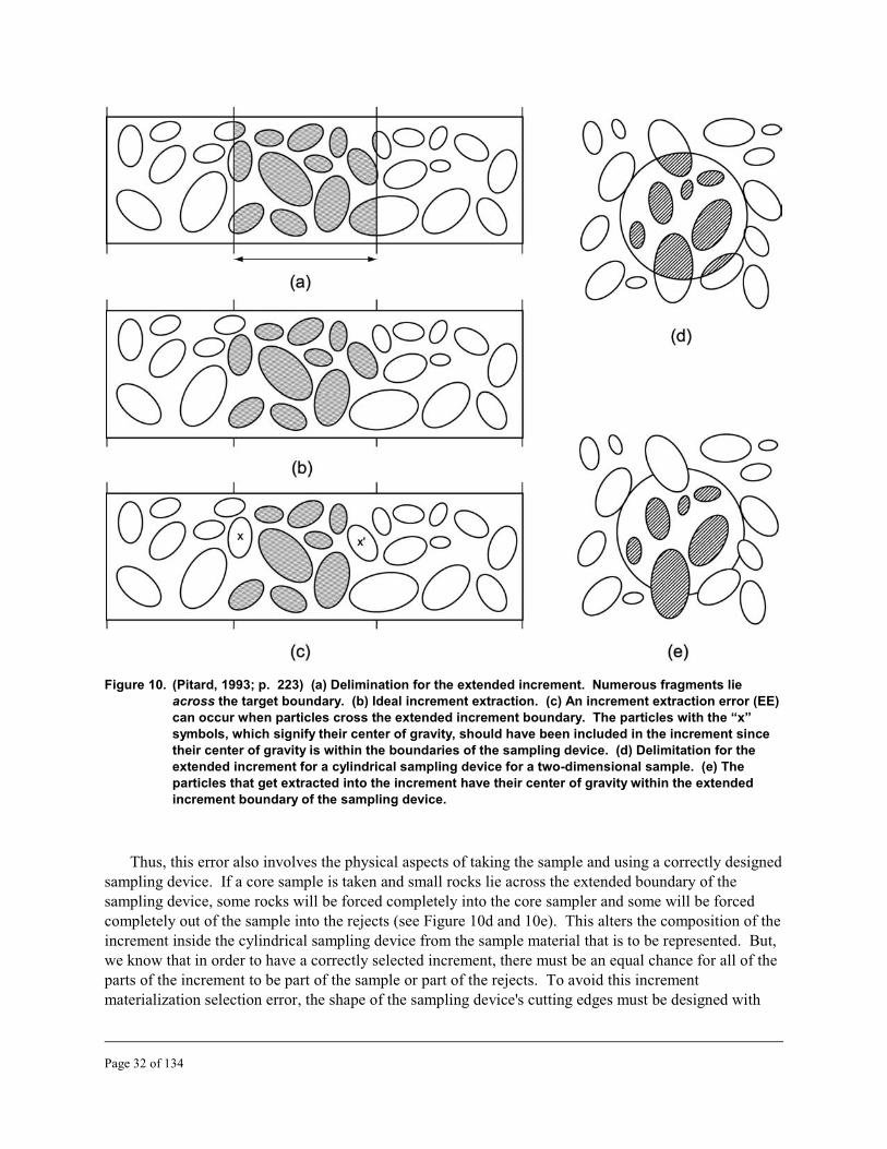
Figure 10. (Pitard, 1993; p. 223) (a) Delimination for the extended increment. Numerous fragments lie

across the target boundary. (b) Ideal increment extraction. (c) An increment extraction error (EE)

can occur when particles cross the extended increment boundary. The particles with the “x”

symbols, which signify their center of gravity, should have been included in the increment since

their center of gravity is within the boundaries of the sampling device. (d) Delimitation for the

extended increment for a cylindrical sampling device for a two-dimensional sample. (e) The

particles that get extracted into the increment have their center of gravity within the extended

increment boundary of the sampling device.

Thus, this error also involves the physical aspects of taking the sample and using a correctly designed sampling device. If a core sample is taken and small rocks lie across the extended boundary of the sampling device, some rocks will be forced completely into the core sampler and some will be forced completely out of the sample into the rejects (see Figure 10d and 10e). This alters the composition of the increment inside the cylindrical sampling device from the sample material that is to be represented. But, we know that in order to have a correctly selected increment, there must be an equal chance for all of the parts of the increment to be part of the sample or part of the rejects. To avoid this increment materialization selection error, the shape of the sampling device's cutting edges must be designed with

Page 32 of 134

respect to the center of gravity of the particle and its chance to be part of the sample or part of the rejects (see Figure 11). The sampling device should go completely through the pile or surface and at a slow, even rate. A rule of thumb for correctly collecting an increment with respect to the increment extraction error is that the inside diameter of the sampling device should be at least 3 times the diameter of the largest particle.

Figure 11. For correct increment extraction, the shape of the sampling

device's cutting edges must be designed with respect to the

center of gravity of the particle and its chance to be part of the

sample or part of the rejects. The sampling device should go

completely through the pile or surface and at a slow, even rate

and the inside diameter of the sampling device should be at

least 3 times the diameter of the largest particle.

There is a practical limit on how small the increment can be for a correctly designed sampling device to remain correct with respect to the increment extraction error, and it has to do with the size of the space of the inner walls of the sampling device. Obviously, this space must be large enough to accommodate the diameter of the largest fragments to be sampled. Not immediately obvious, however, is that the action of the cutter moving through the sample could cause some of the fragments that should be part of the increment (that is, those fragments that have their center of gravity within the increment extended boundary) to move from the leading cutting edge making contact with those fragments to past the opposite trailing cutting edge if that space is too small. Therefore, those fragments do not become part of the sample and the quest for a fragment to have an equal chance to be part of the sample or to not be part of the sample is lost, and a sampling bias is introduced. Pitard (1993, pp. 292 ff) gives several rules for cutter speed and inner wall sampler width. Those rules are generally summarized giving: a maximum cutter speed of 0.6 m/s; an inner wall sampler width of 3d for coarse materials (d $3 mm) and 3d + 10

Page 33 of 134

mm for very fine materials, thus giving a minimum of 10 mm; and a sampler depth of at least 3d. The cutting angle should be either zero (the cutting edge is perpendicular to the extended increment) or greater than or equal to 45 degrees. Those rules may be quite constraining for the very small increments that may be needed for laboratory subsampling. If a width of less than 10 mm is used, we can only suggest (without our own empirical evidence) that the cutter speed should be much slower.

For riffle splitters, Pitard (1993, p. 302) recommends a correct riffle chute width of 2d + 5 mm. No minimum width is recommended for sectorial splitters, although an opening somewhat larger than d is obvious; however, Pitard (1993, p. 303) does recommend that the sector slope should be at least 45° for dry materials and 60° for slightly moist materials. Since true splitting methods select the splitting increments at random, the extraction bias (EE) should cancel out for those methods.

2.13 The Preparation Error (PE) – Sample Integrity

Gy theory identifies error associated with sample integrity as the preparation error (PE; see Table 2). This error involves: gross errors, such as losses, contamination, alteration (e.g., sample degradation); uncertainty added during sample handling, shipping, storage, preservation; or any process that could alter the analyte level between when the sample is obtained and when it is analyzed. This error can be minimized by being careful, being honest, and using common sense. This does not include the error from a chemical extraction step performed as part of a chemical analysis (Gy theory would identify that error as part of the analytical error, AE). A listing of the most common PE types is shown in Table 3.

Page 34 of 134

Table 3. Mechanisms for increased bias and variability due to sample integrity and the PE.

Area of Concern Examples

Contamination C Dust from other samples (Schumacher et al., 1990).

C Cross-contamination from sampling equipment; e.g., drill corer not

C cleaned between borings.

Carryover from previous sample via contaminated analysis equipment.

C Addition of material from abrasion of sampling/preparation equipment;

e.g., trace Cr analysis after using stainless steel sampling apparatus.

C Addition of material from corrosion of sampling/preparation equipment.

Chemical modification C Reactions adding material; e.g., oxidation of sulfur.

C Loss of chemical constituents; e.g., starting with a hydrate and ending

C with an anhydrate.

Analyte binding to sample container or processing equipment.

Physical alteration C Addition of a critical component; e.g., absorption of water.

C Loss of a critical component; e.g., evaporation of elemental Hg or volatile

organic compounds.

C Loss due to heating. Volatile and semi-volatiles lost while grinding the

sample.

C C

Dust lost preferentially, reducing or enriching a constituent.

Loss of material in processing equipment; e.g., very fine grinding of gold

C bearing rocks containing elemental gold results in gold-plated equipment.

Unequal loss of material by fraction or type.

Biological alteration C Microbial consumption of organic constituent.

Unintentional mistakes C Dropping the sample.

C C

Mixing labels.

Equipment failure.

C C

Error in implementing the method.

Transcription error.

Intentional error C C

Fraud.

Sabotage.

2.14 The Importance of Correctly Selected Increments

As the number of increments, N, taken “correctly” from the sample increases, the relative variance 2due to the grouping and segregation error, sGE , decreases. However, there is a point of diminishing

returns. The limitation for increments is to subsample one particle at a time; that is, one increment equals one particle.

The relative variance of the short-range fluctuation error, sCE12, can be minimized to be about the

magnitude of the fundamental error if more increments are taken for each subsample. Recall that

2sCE12 = sFE

2 + sGE .

Page 35 of 134

For most cases, one can assume (Pitard, 1993; p. 189) that

sGE2 # sFE

2

Then

2 2sCE12 = sFE

2 + sGE # 2 sFE .

(Note that this is not always true; for example, a sample made of only one increment containing a highly 2 2segregated fine material may have a very small s but a much larger s ). Then, for N increments, FE GE

taken with correct sampling practices, we can write (Pitard, 1993, p. 388)

sGE2 . sFE

2 / N

and

2 2 2sTE2 $ sCE1 # sFE + [s / N]. FE

2 2Thus, one can see that sTE $ sCE12 . sFE if N is made large enough. At least N = 30 increments are

2 2recommended as a rule of thumb to reduce sGE compared to s (Pitard, 1993; p. 187). FE

A grab sample may consist of one large increment. Grab sampling is an incorrect procedure because it consists of just one increment, taken with judgement and taken incorrectly (without respect to minimizing the GE, DE, and EE). It is incorrect because most particulate samples are impossible to mix so that all of the particles are available to the grab sample with the same probability. However, in addition to being incorrectly taken, the single increment grab sample will include some correlation (because of GE) between particles in the selected and in the unselected components, which is related to increased bias and uncertainty. In a sense, correct sampling is a requirement that produces the correct mean value over the long term. However, there are many different ways to obtain the correct mean value, and each is associated with a different variability. Correct sampling by itself does not guarantee low sampling error (because of the presence of the fundamental error).

Subsampling methods can be roughly ranked with respect to the number of increments they use. The use of many increments is one way to avoid the random effects that leave large fractions of sample with very low or very high concentrations due to problems with fractionation or from random chance.

Figure 12 shows an example where increment sampling overcomes the uncertainty from grouping and segregation effects, demonstrating that certain errors can be reduced by using appropriate subsampling techniques. In this figure, the lot contains 30 “triangular” (in two-dimensions) particles and 10 “circular” particles, giving a ratio of 3.0 for triangular-to-circular particles. The GE in this lot is significant, and any one of the three increments (say, acting as a “grab” sample) does not represent that ratio very accurately. The ratio for increment 1 is 1.25, the ratio for increment 2 is 8.0, and the ratio for increment 3 is 1.33. However, after the three increments are combined to make the sample, the ratio is “averaged out” to 2.125, which is much more “representative” of the lot ratio of 3.0.

Page 36 of 134

Figure 12. This highly segregated lot is randomly sampled with increments of the

same total area. None of the increments alone represent the lot very

well; however, when combined (thus, reducing GE), the sample is much

more representative of the lot.

The concept of many increments can be extended to include particle size. Large particles can be thought of as large increments. Having selected one part of the particle, one automatically gets the other part. The mass components making up a large particle can be thought of as intrinsically correlated fragments. The correlation between parts of a large fragment is similar to the correlation between particles taken as part of an increment or with a scoop in various subsampling procedures. The correlation between different mass components, whether between or within particles is a key indicator for the level of uncertainty obtained with any subsampling method. Sampling methods that minimize correlation among all mass fragments will help to minimize uncertainty.

2.15 Increment Sampling and Splitting Sampling

The increment selection process and the splitting selection process are both sampling (mass reduction) techniques that involve taking correctly selected increments, using correctly designed sampling tools, and combining those increments to form the (hopefully representative) sample. But, there is a fundamental difference between the two techniques. For the increment sampling process, the selection of where and how to take the increment occurs before the actual materialization (the delimitation and the extraction of taking that increment, and the combination of those increments to form the sample as they are sequentially taken). For the splitting sampling process, the fractions are first correctly delimited; however, the selection of which fractions (the splits) to use as the sample or to combine to make the sample occurs after the extraction of those fractions. Thus, even if the fractions are systematically or technically biased, if the fractions or the splits are chosen at random, the bias should average out to be negligible. In the increment sampling process, the increments have already been sequentially selected and combined to make the sample; that is, the selection of the increments preceded

Page 37 of 134

the materialization (formation) of the sample, so that there is no “turning back.” Hence, it is very important that the increments are taken correctly and are technically unbiased for increment sampling. The difference between increment sampling and split sampling is clearly illustrated in the case studies section, called, “Case Study: Increment Subsampling and Sectorial Splitting Subsampling.” This difference of the random selection of fragments can be an advantage for the splitting sampling methods. Some splitting methods combine the best of both the increment and the splitting sampling processes. For example, each fraction from a sectorial splitter (see section on sectorial splitters under “Subsampling Techniques”) is made up of many small increments, yet the fractions that are selected to make up the sample can be chosen at random.

2.16 Correct Sampling (Correct Selection) Defined

The endeavor to reproduce a subsample having the same physical and chemical constitution as the parent sample gives confidence that the subsample has reached the minimum relative variance of the

2fundamental error (s ) that was present in the parent sample. The effort to reproduce the same particle FE

size distribution in the subsample as in the parent sample is enacted by:

C Minimizing the effect of the grouping and segregation error (GE) by correctly taking andcombining many random increments.

C Minimizing the effect of the delimitation error (DE) by using a correct sampling device that can extend through the sample to give an increment volume selected to give each constituent of the sample an equal chance to enter the boundaries of that sampling device. That correctly delimited sampling device would be a scoop with parallel sides and a flat bottom for a sample in a one-dimensional (one long dimension) pile or a cylinder with a constant cross section for a two-dimensional (two long dimensions) sample.

C Minimizing the effect of the extraction error (EE) by using a correct sampling device that, as it cuts through the correctly delimited increment, gives each constituent an equal chance of being selected as part of the increment or not. Thus, a correctly designed sampling device must have cutting edges that allow, with equal probability, the constituent to be part of the increment if its center of gravity is within the extended bounds of correct delimitation, or the constituent not to be part of the increment if its center of gravity is outside of the extended bounds of correct delimitation.

C Minimizing the effect of the preparation error (PE) – those “human” mistakes, such as contamination, losing some sample, or altering the composition of the sample – by being careful, honest, and using common sense.

Correct sampling practices, therefore, challenge us to minimize those errors that we have some control 2 2 2 2 2over (that is, mTE , sGE , sDE , s , and s become negligible) so that we can produce a subsample that EE PE

has the same intrinsic minimum relative variability (sFE2) inherited from the original parent sample.

Page 38 of 134

2.17 Representative Sample Defined

A goal of the Gy sampling theory is to obtain a representative sample, defined as a sample that is both accurate (within a specified level of bias) and precise (within a specified level of relative variance) at the same time (Pitard, 1993; p. 415). The degree of representativeness, r 2, is given by TE

2rTE2 = m TE

2 + sTE

2 2where TE is the total sampling error, r is the mean square of the total sampling error, m is the square TE TE 2of the mean of the total sampling error, and sTE is the relative variance of the total sampling error. The

total sampling error, TE, refers to the relative difference between the expected (true or assumed) value of the proportion of the analyte in the lot, a , and the estimated value of the proportion of the analyte in the L

sample, a , when there is preparation error, PE: s

Note that TE = SE + PE = CE + ME = FE + GE + CE + CE + DE + EE + PE. 2 3

A subsample should be representative of the sample it was taken from and be an estimation of the original lot, as defined by the study objectives (e.g., data quality objectives, DQOs) and the sampling plan. In the case of laboratory subsampling, the analytical subsample (e.g., for chemical analysis) must be representative of the entire contents of the laboratory sample bottle.

A sample is representative when

2rTE2 # roTE

where roTE2 is a specified and quantitative measure of a representative sample (the smaller this number,

the more representative is the sample); that is, it is a level of representativeness regarded as acceptable.

But, without knowing a , can we know how representative our samples are of the lot? Yes, weL 2should be able to using the strategy that the bias is negligible (mTE = 0) and the “controllable” relative

variances are minimized when the sampling practices are perfectly correct (that is, when GE = DE = EE 2 2 2= PE = 0). It is desirable to keep s # soTE , where s is a level of the relative variance of the total TE oTE

2sampling error within user specifications. If sampling practices are perfectly correct (that is, s = sDE2 = GE

2sEE2 = sPE

2 = 0), then s = sFE2 (the relative variance of the fundamental error). Thus, if correct sampling TE

practices are applied and all of those “controllable” errors are minimized, then a representative sample could be characterized by keeping the relative variance of the fundamental error below a specified level,

2sFE2 # soFE . Under such conditions,

2rTE2 . sFE

2 # soFE . roTE2

This equation will serve as the basis of our strategy to obtain a representative subsample for chemical analysis. This is fortuitous for our planning purposes, and for formulating our study objectives (e.g.,

2DQOs), since sFE is the only error that can be calculated, based on the physical and chemical properties of the particulate material, a priori; that is, before sampling even takes place!

Page 39 of 134

As can be seen from the above definition, like heterogeneity, and because of its relationship to heterogeneity, representativeness is a matter of scale and depends on the focus and requirements of the user. Thus, the user should now have a logical approach (and a sampling strategy) to specifying the tolerable amounts of bias and variability (set in the DQOs).

Page 40 of 134

Section 3

Fundamental Error Fundamentals

The fundamental error is the minimum sampling error generated even when all of the sampling operations are perfect. The fundamental error is a result of the constitution heterogeneity of the materials making up the lot, those materials being chemically or physically different. When correct sampling practices are used (that is, GE + DE + EE + PE . 0) and the long-range fluctuation errors are assumed tobe negligible for laboratory subsampling (that is, CE + CE 3 = 0 ), the fundamental error can be 2

expressed as a proportion of the true mean for the lot being sampled:

where a is the actual content of the analyte in the lot and a is the measure content of the analyte in the L s

sample. The mean of the fundamental error (under the above conditions) is expected to be negligible; that is,

The relative variance of the fundamental error, under the above conditions, can be expressed as:

Estimation of the relative variance of the fundamental error provides a baseline from which one can plan a subsampling strategy that can meet the study DQOs. Several examples and test cases are provided to demonstrate both the estimation methods and how to use the information once it is acquired.

3.1 Estimating the Relative Variance of the Fundamental Error, s 2 FE

Several formulas have been developed as approximate estimates of the relative variance of the fundamental error. Each formula is the result of a number of approximations and assumptions. While the assumptions may not always be exact, the results are often still useful as an aid in making sampling decisions.

Page 41 of 134

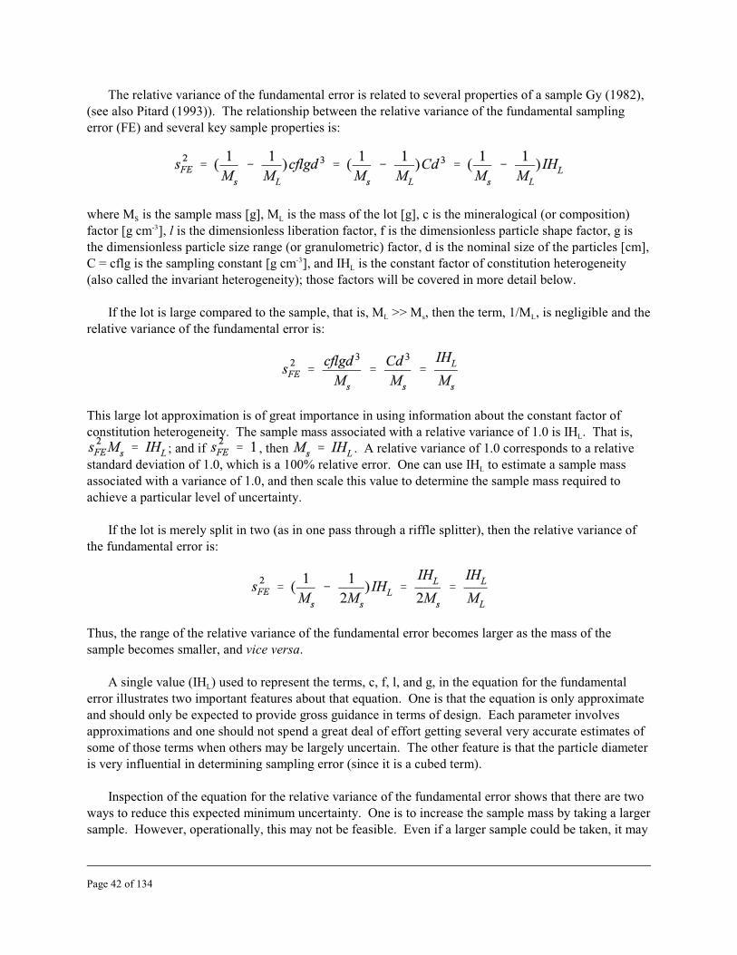
The relative variance of the fundamental error is related to several properties of a sample Gy (1982), (see also Pitard (1993)). The relationship between the relative variance of the fundamental sampling error (FE) and several key sample properties is:

where M is the sample mass [g], M is the mass of the lot [g], c is the mineralogical (or composition)S L-3factor [g cm ], l is the dimensionless liberation factor, f is the dimensionless particle shape factor, g is

the dimensionless particle size range (or granulometric) factor, d is the nominal size of the particles [cm], -3C = cflg is the sampling constant [g cm ], and IH is the constant factor of constitution heterogeneity L

(also called the invariant heterogeneity); those factors will be covered in more detail below.

If the lot is large compared to the sample, that is, M >> M , then the term, 1/M , is negligible and the L s L

relative variance of the fundamental error is:

This large lot approximation is of great importance in using information about the constant factor of constitution heterogeneity. The sample mass associated with a relative variance of 1.0 is IH . That is,L

; and if , then . A relative variance of 1.0 corresponds to a relative standard deviation of 1.0, which is a 100% relative error. One can use IH to estimate a sample mass L

associated with a variance of 1.0, and then scale this value to determine the sample mass required to achieve a particular level of uncertainty.

If the lot is merely split in two (as in one pass through a riffle splitter), then the relative variance of the fundamental error is:

Thus, the range of the relative variance of the fundamental error becomes larger as the mass of the sample becomes smaller, and vice versa.

A single value (IH ) used to represent the terms, c, f, l, and g, in the equation for the fundamental L

error illustrates two important features about that equation. One is that the equation is only approximate and should only be expected to provide gross guidance in terms of design. Each parameter involves approximations and one should not spend a great deal of effort getting several very accurate estimates of some of those terms when others may be largely uncertain. The other feature is that the particle diameter is very influential in determining sampling error (since it is a cubed term).

Inspection of the equation for the relative variance of the fundamental error shows that there are two ways to reduce this expected minimum uncertainty. One is to increase the sample mass by taking a larger sample. However, operationally, this may not be feasible. Even if a larger sample could be taken, it may

Page 42 of 134

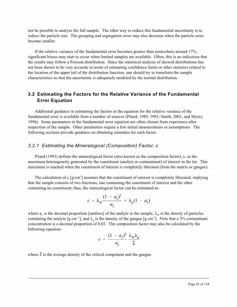
not be possible to analyze the full sample. The other way to reduce this fundamental uncertainty is to reduce the particle size. The grouping and segregation error may also decrease when the particle sizes become smaller.

If the relative variance of the fundamental error becomes greater than somewhere around 17%, significant biases may start to occur when limited samples are available. Often, this is an indication that the results may follow a Poisson distribution. Since the statistical analysis of skewed distributions has not been shown to be very accurate in terms of estimating confidence limits or other statistics related to the location of the upper tail of the distribution function, one should try to transform the sample characteristics so that the uncertainty is adequately modeled by the normal distribution.

3.2 Estimating the Factors for the Relative Variance of the Fundamental

Error Equation

Additional guidance in estimating the factors in the equation for the relative variance of the fundamental error is available from a number of sources (Pitard, 1989, 1993; Smith, 2001; and Myers, 1996). Some parameters in the fundamental error equation are often chosen from experience after inspection of the sample. Other parameters require a few initial measurements or assumptions. The following sections provide guidance on obtaining estimates for each factor.

3.2.1 Estimating the Mineralogical (Composition) Factor, c

Pitard (1993) defines the mineralogical factor (also known as the composition factor), c, as the maximum heterogeneity generated by the constituent (analyte or contaminant) of interest in the lot. This maximum is reached when the constituent of interest is completely liberated (from the matrix or gangue).

3The calculation of c [g/cm ] assumes that the constituent of interest is completely liberated, implying that the sample consists of two fractions, one containing the constituent of interest and the other containing no constituent; thus, the mineralogical factor can be estimated as:

where a is the decimal proportion [unitless] of the analyte in the sample, 8 is the density of particles L M-3 -3containing the analyte [g cm ], and 8 is the density of the gangue [g cm ]. Note that a 3% contaminantg

concentration is a decimal proportion of 0.03. The composition factor may also be calculated by the following equation:

where 86 is the average density of the critical component and the gangue.

Page 43 of 134

For environmental applications where the decimal proportion of contaminant is low (a < 0.1), the L

estimate of the mineralogy factor is further simplified to:

Likewise, when the decimal proportion of contaminant is high (a > 0.9), the estimate of the L

mineralogy factor is simplified to:

The accuracy of these estimates may need to be evaluated in situations where hazardous waste concentrations are close to regulatory levels. However, if just used for planning, the only impact on the study should be the need to implement a design that reflects the increased need for accuracy so that the expected measured levels can be differentiated from the regulatory level.

3.2.2 Estimating the Liberation Factor, l

Because, for the calculation of the mineralogical factor, we needed to assume that the constituent of interest is completely liberated from the gangue (matrix), we now need a correction factor, the liberation factor (l) [dimensionless], for when complete liberation is not the case. Thus, 0 # l # 1. Gy (1998, p. 67) recommends setting l = 1 for environmental samples when no additional criteria are available. For most pollutants, this should be acceptable, as the methods are for total analyte.

Pitard (1993) provides guidance on choosing l based on an assumed degree of heterogeneity of the analyte (Table 4) and gives alternative methods of calculation that rely on the true (estimated as an average) critical content of the constituent of interest (analyte or contaminant) in the lot, a , and the L

maximum critical content of the constituent of interest in the coarsest fragments of the lot, a , where the max

critical content is in terms of the proportional amount of the constituent of interest in the sample. The formula based on the critical contents is:

This equation assumes that one knows the maximum critical content, a , that all size fractions have max

approximately the same critical content, a , and that, for each fraction, the critical constituent is L

segregated into individual particles.

Page 44 of 134

Table 4. Liberation parameter estimates by material description.

l Type of Material

1.0 Analyte 100% available (recommended for most environmental applications when no criteria

are available)

0.8 Very Heterogeneous

0.4 Heterogeneous Material

0.2 Average Material

0.1 Homogeneous Material

0.05 Very Homogeneous Material

If one has a mineral-like analyte, then the liberation factor can also be estimated by (Gy, 1982):

where d is the diameter needed to liberate the contaminant. Francois-Bongarcon and Gy (1999) l

developed a generalized version of this last equation, expressed as:

where b is an adjustable parameter that needs to be estimated for each application for the best results. For most mining applications, where metal grains are distinct from the surrounding matrix, the value of b is 3/2.

These equations should only be used for samples where the analyte of interest exhibits mineral-like properties. In addition, we note that these equations are simplified versions of a more complex model. The estimates assume that the liberation factor takes on only one value for all size fractions unless one can predict how a varies as a function of particle size. max

3.2.3 Estimating the Shape Factor, f

The shape factor, f, also known as the coefficient of cubicity, is a dimensionless measure of how close the particle’s shape is to a perfect cube (where f = 1.0). The shape factor relates volume, V, to a fragment size diameter, d, of unity:

Page 45 of 134

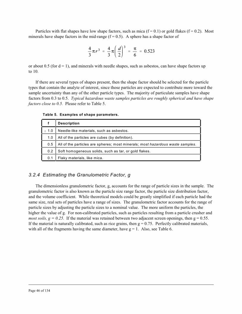
Particles with flat shapes have low shape factors, such as mica (f = 0.1) or gold flakes (f = 0.2). Most minerals have shape factors in the mid-range (f = 0.5). A sphere has a shape factor of

or about 0.5 (for d = 1), and minerals with needle shapes, such as asbestos, can have shape factors up to 10.

If there are several types of shapes present, then the shape factor should be selected for the particle types that contain the analyte of interest, since those particles are expected to contribute more toward the sample uncertainty than any of the other particle types. The majority of particulate samples have shape factors from 0.3 to 0.5. Typical hazardous waste samples particles are roughly spherical and have shape factors close to 0.5. Please refer to Table 5.

Table 5. Examples of shape parameters.

f Description

$ 1.0 Needle-like materials, such as asbestos.

1.0 All of the particles are cubes (by definition).

0.5 All of the particles are spheres; most minerals; most hazardous waste samples.

0.2 Soft homogeneous solids, such as tar, or gold flakes.

0.1 Flaky materials, like mica.

3.2.4 Estimating the Granulometric Factor, g

The dimensionless granulometric factor, g, accounts for the range of particle sizes in the sample. The granulometric factor is also known as the particle size range factor, the particle size distribution factor, and the volume coefficient. While theoretical models could be greatly simplified if each particle had the same size, real sets of particles have a range of sizes. The granulometric factor accounts for the range of particle sizes by adjusting the particle sizes to a nominal value. The more uniform the particles, the higher the value of g. For non-calibrated particles, such as particles resulting from a particle crusher and most soils, g = 0.25. If the material was retained between two adjacent screen openings, then g = 0.55. If the material is naturally calibrated, such as rice grains, then g = 0.75. Perfectly calibrated materials, with all of the fragments having the same diameter, have g = 1. Also, see Table 6.

Page 46 of 134

Table 6. Granulometric factor values identified by Gy (1998).

g Description

0.25 Undifferentiated, unsized material (most soils).

0.40 Material passing through a screen.

0.50 Material retained by a screen.

0.60/0.75 Material sized between two screens.

0.75 Naturally sized materials, e.g., cereal grains, certain sands.

1.0 Uniform size (e.g., ball bearings).

3.2.5 Estimating the Nominal Particle Size, d

The nominal particle size, d, identifies how large the largest particles are in the sample. One estimate for the nominal particle size is the linear dimension (in cm) of a square mesh retaining no more than 5% oversize. Another definition is that 95% of the particles must have linear dimensions less than d. The level of 95% represents a practical compromise that avoids parameter selections based on extremes from observed distribution functions. The value of d should be readily estimated by examination. The influence of d in the fundamental error equation is very high.

3.2.6 Estimating the Required Sample Mass, M s

Several procedures have been proposed to estimate the sample weight required to achieve a study’s DQOs. The two-tiered and Visman procedures may at times be more appropriate for determining field sample requirements than for evaluating laboratory samples; however, those procedures still demonstrate the needs and limitations related to identifying the sample mass. Understanding those requirements will provide two benefits. One is to generate an understanding of alternate types of solutions that are available and when they can be used. The other is to prevent wasted effort on trying to solve this issue when it is not cost effective.

3.2.7 Rearrangement of the Relative Variance for the Fundamental Error

Equation to Determine the Sample Mass (M )s

The most common method of estimating the sample mass, M , utilizes a rearrangement of the S

equation for the relative variance for the fundamental error:

Page 47 of 134

Rearranging gives:

And, if M << M , then: s L

The minimum variance is either known or estimated from the decision criteria that need to be met. The mass of the lot either is known or it can be ignored if it is large compared to the subsample mass. The other parameters are estimated based on the information from the sample, or other preliminary samples, or from reasonable estimates from references or tables (such as Pitard, 1993). This sample mass (M ) estimate is a minimum value, since other sources of error (besides sFE

2) could contribute to the s

overall variance. Thus, a larger mass may be required to meet the DQOs. However, this estimate should prove useful in identifying if a reasonable sample mass will provide the necessary information.

3.2.8 Two-tiered Variance Comparison to Estimate IH and the Sample Mass L

(Ms)

Estimating IHL can be used to determine the required sample mass using a two-tiered variance comparison and is discussed in Pitard (1993, pp. 363, 386) and Meyers (1997). It is most appropriately applied to cases involving 2-dimensional and 3-dimensional lots, but may also provide information for zero-dimensional and one-dimensional lots. Although this method may be limited in the application to producing representative laboratory analytical subsamples (the subject of this guidance), it is presented here because this method can be used to characterize the type and amount of heterogeneity and it is a way to optimize a sampling plan.

The number of samples and analyses associated with this procedure result in time and analysis expenses that are justified only under certain circumstances. Any one of the following conditions might justify the use of this method.

C A large number of similar samples are expected.

C A large economic expense is associated with the decisions based on the analysis results.

C The time and cost for an analysis is low.

Two sets of samples are required, with one sample for each set taken from the same location. Pitard recommends the number of samples to be N = 50 (Pitard, 1993, p. 365), but reasonable estimates are expected for sample sizes down to N = 30 (note that each sample is made up of at least 10 random increments). However, if 30 samples are prohibitive, Pitard (1993, p. 385) suggests using only 10 samples per set. While 10 is too low to produce a close estimate of the uncertainty, it is large enough to identify the order of magnitude for the sampling uncertainty.

Page 48 of 134

Assume that the mass of each sample in the first set is M , and the mass of each sample in the second s1

set of samples is M , with M $ 10Ms1. The larger mass can be as large as 100 times the smaller mass s2 s2

without affecting the comparison. Each sample must now be analyzed in its entirety. No subsampling is allowed. This restriction often limits the upper sample mass level. A test sample should be run to check the compatibility of the sample mass with the analytical method.

The variance for both sets of samples is now estimated and compared. There are four possible outcomes:

Case 1. .

This is the most likely outcome. It means that effects such as grouping and segregation errors differ over the scale change in mass. The conclusion is that mass is important. The recommendation is that the sample weights should be based on the larger mass. One consequence is that the small mass samples should be ignored while the larger mass sample results can be retained as part of the study.

Case 2. , and both are small.

This outcome is rare and arises if the material is relatively homogeneous. The conclusion is that the small mass is acceptable for characterizing the sample. However, one should realize that this outcome can also occur when both sample sizes present estimates of the background concentration, and neither sample mass was collected in an area with high levels of the hazardous substance. This may occur if the contaminant occurs at only a few locations within the lot, or if both sample sizes are small with respect the size of the lot and the contaminant is distributed like a series of discrete points rather than continuously affecting the entire area. Assuming that the small mass does give acceptable results, then both sets of results may be retained.

Case 3. , and both are large.

This outcome suggests that sample mass is not a primary source of variance and usually is a result of a low concentration of pollutant or large fragments, or the effects of the heterogeneity fluctuation errors, CE2 and CE3, in the field. The variance estimates probably represent the large-scale heterogeneity of the matrix. The conclusion that sample mass is not important implies that the small mass level may be adequate. Again, both sets of results can be retained as part of any further work.

Case 4. .

This outcome means that both of the sample masses are too small. The only conclusion is that an acceptable result requires a sample mass greater than M . None of the results should be retained as part 2

of the study. Another set of samples with a larger mass M should be run. Pitard (1993, p. 387) s3

recommends that Ms3 = 10 Ms2 be selected. One can also compare the average concentrations. If the average concentration of the smaller masses is lower than the average concentration of the larger sample masses, then the smaller samples cannot be representative of the low occurrence of pollutant or low-frequency pollutant clusters.

Page 49 of 134

3.2.9 Visman Sampling Constants Approach for Determining the Sample Mass

(Ms)

Visman (Visman, 1969; and Myers, 1996, p. 440) introduced two sampling constants, A and B, that can be used to estimate the optimal and the minimum sample weight. Sampling constant A is related to the heterogeneity of the sample and sampling constant B represents the variance effects from segregation, grouping, long-range fluctuations, and periodic fluctuations. Using the summary information from the two sets of samples with different masses described in the section, entitled “Two-tiered Variance Comparison to Estimate IH and the Sample Mass (M ),” the Visman sampling constants can be L s

calculated as:

The optimal sample weight (Ingamells and Switzer, 1973; Ingamells, 1974; and Ingamells and Pitard, 21986) is MsOpt = A/B, and the minimum sample weight is M = A/(a – aB) , where a is the background sMin 1 B

concentration and a1 is the average concentration in sample set 1.

3.3 Developing a Sample Mass or Comminution Strategy: The Sampling

Nomograph

Gy sampling theory provides a relatively easy way to develop a sample mass or comminution strategy, or to optimize a sampling protocol (e.g., to stay within the predefined error limit set by the DQO process) using a sampling nomograph (Pitard, 1993, and Myers, 1997). One of the key results from the Gy sampling theory is the relationship between the relative variance of the fundamental error (sFE

2), the particle size (d), and the mass of the sample (M ). The sampling nomograph is a two-dimensional s

summary of this relationship among the three factors in the fundamental error equation:

If we assume that the mass of the lot is very large compared to the mass of the sample, , then:

where C is termed the sampling constant. Because it is cubed, the particle size obviously plays a key role when estimating the fundamental error. The development of this equation included several assumptions,

Page 50 of 134

so one must remember it is only an approximate relationship. However, for most particle samples, the assumptions are justified. The above equation is now recast by taking the logarithm (base 10) of each side, resulting in:

This equation shows that, for a given particle size, d, plotting the logarithm of the relative variance of the fundamental error versus the logarithm of the sample mass gives a straight line with a slope of minus one. This equation will be used to construct the sampling nomograph.

3.3.1 Constructing a Sampling Nomograph

Figure 13 shows a sampling nomograph and the following example explains how to construct and use it. To create a nomograph one has to identify at least one solution to the last equation. (Any solution to the relative variance of the fundamental error equation will do. Typically, one knows the largest value of d and the maximum sFE1

2 is usually set through the DQO process; the value of M is calculated from the S

equation for the relative variance of the fundamental error.) This solution specifies the diameter associated with some combination of the relative variance of the fundamental error and the sample mass. The relative variance of the fundamental error and the sample mass determine the location of a point on the sampling nomograph. A line with slope of -1 is then drawn through this point and labeled with the particle diameter.

It is the placement of the slope diameter lines that makes each nomograph different. By changing d and keeping either the relative variance of the fundamental error or the sample mass constant, additional points can be found and a series of lines representing different particle diameters can be drawn. The positions of these lines all have some uncertainty associated with them and the nomograph is only as good as the model used to construct it. The farther away one goes from the original point, the more uncertainty that there is in the predictions from the nomograph. One should try to use the nomograph in areas as close to the initial point as possible. For more accurate predictions, additional points should be identified from independent examples instead of extrapolating from the single point.

The assumptions made using the starting equation (the log10 of the relative variance of the fundamental error equation) include:

C The sample mass is small compared to lot mass

C The estimates of the parameters used to calculate the sampling constant are reasonably accurate

The assumptions made when deriving the starting equation include (Myers, 1997, Appendix C; Pitard, 1993; and Gy, 1982):

C An average fragment mass is used

C The critical content of all of the fractions with a given density is set to the average critical content for that density fraction

C The proportion of the mass of a size density fraction in the lot to the mass of the density fraction in the lot is replaced by the proportion of mass of the size fraction of the lot to the mass of the lot

Page 51 of 134

Figure 13. An example of a sampling nomograph.

The sampling nomograph uses log-log coordinates (and, therefore, can be plotted on log-log paper). The sampling nomograph has an x-axis for the sample mass that is logarithmic in scale [log10 grams]. Each major vertical grid line represents a 10-fold change in mass. The y-axis is the base 10 logarithm of the fundamental error in [log relative variance units]. A bold horizontal line may be drawn in to 10

represent the maximum relative variance of the fundamental error that is tolerated, as set by the study objectives (e.g., DQOs). The family of slanted lines (each with a slope of -1) represent the diameter (d) of the largest particle size in a given sample. The distance between the slanted parallel lines is also logarithmic (base 10). A vertical drop from a point on one slanted line to the point below on another slanted line indicates a comminution stage (d becomes smaller). Going from one point (representing a larger mass) on the slanted line to another point (representing a smaller mass) indicates a subsampling stage (d and IH remain constant; M becomes smaller). Using various comminution and subsampling L s

stages (that is, going from point-to-point along the various slanted lines) to achieve the final subsample mass while staying within our maximum tolerated relative variance comprises our subsampling strategy.

Page 52 of 134

3.3.2 Hypothetical Example

A sample has been evaluated and it is represented in Figure 13 at point A. The sample at point A has a mass of 763 g, with the largest particle being about 0.3 cm. A preliminary screening analysis of other samples from the lot to be represented by this sample revealed that the average content of the

-4contaminant is about 100 ppm; that is aL = 0.0001 = 10 . The contaminant, metallic lead, has a density -3 -5of 8M = 11.4 g cm . The liberation diameter was determined to be dl = 9.5 x 10 cm. The factors for the

relative variance of the fundamental error for this sample are:

Ms = 763 g aL = 0.0001 = 10-4

8M = 11.4 g cm-3

-4 5 -3c = 8M / a = (11.4 g cm-3 / 10 ) = 1.14 x 10 g cm L

f = 0.5 g = 0.25 d = 0.3 cm dl = 9.5 x 10-5 cm

-5 ½l = (d / d)½ = (9.5 x 10 cm / 0.3 cm) = 0.018 l

C = cflg = 254 g cm-3

Assuming that the sample came from a much larger lot (i.e., M >> M ), the relative variance of the L s

fundamental error for the sample is:

3 -3 3 -3sFE2 = Cd / Ms = (254 g cm )(0.3 cm) / 763 g = 9 x 10

The study design objectives require an analysis using a maximum of 5 g of material with a maximum 2 -3 relative variance for the fundamental error of 0.00625 or sFE = 6.25 x 10 . The analytical method has an

uncertainty (CV) of less than 5% (RSD = 0.05), or a maximum relative variance of (0.05)2 = 2.5 x 10 , 2which is only somewhat smaller than the maximum sFE tolerated by the study objectives. Note that both

-3the relative variance for the fundamental error (9 x 10 ) and the mass (763 g) for the sample are larger 2 -2 than the requirements set by the study objectives (a maximum s of 6.25 x 10 and an analytical sample FE

mass of 5 g). This is clearly the case when looking at point A on the sampling nomograph in Figure 13. Thus, in order to meet the study objectives, the sample needs to be altered by a subsampling and comminution strategy, which can be developed using the sampling nomograph.

The path from point A to point E on the sampling nomograph in Figure 13 may be a route that can be followed to get to the 5 g analytical sample. The first step is to go to point B. The only difference between point A and point B is that the maximum particle size is smaller. Grinding (the comminution stage) the sample until the largest particle diameters are no greater than 0.1 cm moves the sample location from point A to point B on the sampling nomograph. Note that when d is changed, as in the

½comminution stage, the liberation factor also changes because of the relationship, l = (d / d) . This alsol

means that the sampling constant, C, changes since C = cflg.

A microscopic inspection of the ground material revealed that, because of the malleable nature of the lead, a change in the liberation diameter may have occurred. A mineralogical investigation showed that the largest particles (0.1 cm) of the ground material contained a maximum metallic lead content of

Page 53 of 134

-3

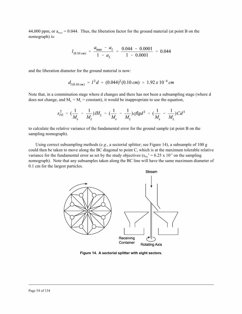
44,000 ppm, or amax = 0.044. Thus, the liberation factor for the ground material (at point B on the nomograph) is:

and the liberation diameter for the ground material is now:

Note that, in a comminution stage where d changes and there has not been a subsampling stage (where d does not change, and M = M = constant), it would be inappropriate to use the equation, L s

to calculate the relative variance of the fundamental error for the ground sample (at point B on the sampling nomograph).

Using correct subsampling methods (e.g., a sectorial splitter; see Figure 14), a subsample of 100 g could then be taken to move along the BC diagonal to point C, which is at the maximum tolerable relative

2 -3 variance for the fundamental error as set by the study objectives (s = 6.25 x 10 on the sampling FE

nomograph). Note that any subsamples taken along the BC line will have the same maximum diameter of 0.1 cm for the largest particles.

Figure 14. A sectorial splitter with eight sectors.

Page 54 of 134

Grinding the 100 g sample to a size of no more than 0.03 cm moves that intermediate subsample from point C to point D. Again, because of the malleable nature of the lead, another microscopic inspection of the ground material revealed another possible change in the liberation diameter. Another mineralogical investigation showed that the largest particles (0.03 cm) of the ground material contained a maximum metallic lead content of 65,000 ppm, or amax = 0.065. Thus, the liberation factor for the ground material (at point B on the nomograph) is:

and the liberation diameter for the ground material is now:

Correctly subsampling from that 100 g subsample along the diagonal line DE until 5 g is reached brings that final analytical subsample to point E on the sampling nomograph with an sFE

2 = 5.0 x 10 , -3 which is below the maximum set by the study objectives (s 2 = 6.25 x 10 ). FE

However, each subsampling event is associated with a minimum addition to the starting point uncertainty (propagation of error). The total relative variance of the fundamental error for this subsampling strategy is the sum of the relative variances of the fundamental error for each subsampling stage along that strategy path; that is, from points A to E, the subsampling stages are the line from point B to point C and the line from point D to point E.

From point B to point C:

From point D to point E:

Page 55 of 134

-3

The total relative variance of the fundamental error for the subsampling strategy as displayed in the sampling nomograph (Figure 13) is:

2 -3 which is above the study objective of a maximum s = 6.25 x 10 . At this point, there are a couple of FE

choices to be made. One is to revise our subsampling and comminution strategy (the path on our 2 -3 nomograph) to stay well below the maximum sFE = 6.25 x 10 with the propagation of error. The other

choice is to revise the study objectives to be more realistic. It is expected that the sampling error (or the maximum sFE

2), even when using correct sampling practices, would be quite a bit greater than the analytical error. A more reasonable error might be a CV of 15% for the fundamental error; that is, s = FE

2 -2 0.15, or a maximum sFE = 2.25 x 10 .

The relative variance of the overall estimation error, sOE2, for this example can be calculated, where it

is assumed that the relative variance of the total sampling error, sTE2, has been minimized by correct

sampling practices relative to the (propagated) relative variance of the fundamental error, sFE2, (that is,

2 2sTE2 . sFE ) and the relative variance analytical error, s , adds to the additive overall variance model: AE

2 2 -2 -3 -2sOE2 = sTE

2 + sAE = sFE2 + sAE = 1.02 x 10 + 2.5 x 10 = 1.27 x 10

The square root of this relative variance of the overall estimation error gives the relative deviation of the overall estimation error:

2 ½(s ) = sOE = 0.11 OE

or a CV (%RSD) of 11%.

3.3.3 Some Subsampling Strategy Points to Consider

Because comminution is often more laborious than subsampling, the best practical strategies would minimize the number of comminution steps. Once an initial point has been identified, the nomograph is a simple aid in identifying the appropriate sample processing strategies (e.g., to stay under the desired maximum relative variance for the fundamental error of 0.0625, as in the example, above). To summarize:

C One cannot expect errors that are smaller than the fundamental error. Estimating the fundamental error provides the benchmark so that one does not waste effort from trying various methods to achieve lower uncertainty levels than are physically possible. If the fundamental error is larger than required by the study objectives for a given sample mass, M , then sample comminution (to s

reduce d) should be carried out following a sampling nomograph strategy. Do not neglect the propagation of error for each subsampling stage when formulating study objectives.

Page 56 of 134

C The grouping component of the error is zero when each fragment is independently and randomly selected. This is not usually a very practical alternative. The practical action is to maximize the number of increments (or splits) and to select those many increments from locations randomly distributed throughout the sample (or lot). Methods with a large number of increments (N $ 30) that select particles representative of the entire sample should produce the best results.

C Mixing the sample is not a guarantee that segregation effects have been eliminated. This means that subsampling methods which minimize or eliminate segregation effects are preferred (again, through many increments or splits taken with correct sampling practices).

C One can modify the equation of the relative variance of the fundamental error used to generate the sampling nomograph if M is on the order of ML; e.g., for one pass through a riffle splitter, M = s L

2M and s

3.4 Low Analyte Concentration Considerations

3.4.1 Low-frequency of Analyte (Contaminant) Particles

It is important to determine if low numbers of contaminant particles are present. If a sparse analyte distribution is not identified, then it is all too easy to misjudge the contamination level of the lot as nonexistent. When only a rare occurrence is the cause of contamination (for instance, the occasional presence of a lead shot), then it is probable that analyzing only a few of the possible subsamples may miss the contaminant. When the fraction of particles containing the contaminant is very small, the distribution of the results is usually more like a Poisson distribution than a Gaussian distribution, and the parameter estimates, such as the mean, will have relatively large uncertainties if only a few results are available. These difficulties may be minimized if the sample mass is increased so that at least 4 or 5 analyte particles are expected in each subsample (Pitard, 1993, p. 370), although, at the very least, 6 analyte particles are recommended (or the estimate of the average analyte concentration may be poor). For laboratory samples this rule-of-thumb would have to be applied based on prior knowledge about the number and distribution of analyte particles. Either the frequency of the analyte particles needs to be known from a prior study or additional representative samples need to be provided to the laboratory for a few test runs.

Sparse distributions of high concentration analyte particles are one of the more difficult sampling problems. The increased relative variability is easily envisioned for cases where only 1 or 2 analyte particles, on average, may end up in a subsample. When only a handful of target particles is involved, it is quite possible for samples to contain no analyte particles, just one particle, 3 particles, or even 5 particles. The relative variability in estimating the overall analyte level would be expected to be very high. Even more important, if less than one particle is expected per subsample, most subsamples might contain no particles and occasionally a sample with one or more particles would be analyzed, resulting in a high analyte concentration.

Page 57 of 134

Sample matrices fitting this description could be repeatedly sampled and subsampled and only rarely would a concentrated particle be selected. A histogram of the analytical results might be highly skewed, with the majority of results at very low concentrations. The occasional very high concentration would appear, for all intents and purposes, as an outlier. If the sparse nature of analyte particles in the sample is not understood, then decisions may be based on the assumption that the data follow a normal probability distribution. Declaring the one subsample with relatively high analyte levels to be an outlier might easily lead to the incorrect conclusion that a contaminated site has met cleanup standards. This is why it is important to determine how the analyte is distributed among the sample particles. If the sample characteristics fail to match the statistical assumptions, then the resulting decisions may not be justified or correct.

Of course, there may be instances when a high value really is an outlier due to random chance (one just happened to select a subsample with very rare high-level contaminant concentration) or to an inadvertent error such as transposing numbers when recording a value. The important question is to evaluate the results in light of any other information so that one minimizes making an incorrect decision. If the result of multiple subsample analysis is near zero for most subsamples and very high for just one subsample, then the question to answer is whether or not the high value is large enough to present a problem. This may be the case if the average analyte concentration exceeds a target cleanup standard or if the net amount of hazardous compound present in the high concentration subsample presents a health hazard. However, whether the outlier is false or real, if its presence does not affect the study outcome, then one should note its presence before continuing with the study.

If the outlier results change the study decision, then additional analysis should be carried out. To increase the chance that such concentration patterns are accounted for rather than ignored, one needs to determine when high-concentration analyte particles may be present in low numbers. Several samples, designed to include at least one high level particle with a 90% or a 95% chance, should be taken. Those samples can be ground to eliminate the effect of particle size in the subsampling procedure (or the entire sample can be exhaustively analyzed). If the concentration is significantly higher from these analyses compared to the results from individual subsamples, then one may be dealing with a matrix that not only requires special processing techniques, but also requires special field sampling practices to ensure that the site is correctly characterized.

For a discussion on outliers, please refer to Barnett and Lewis (1995) or to Singh and Nocerino (1995). Software has been developed for the methods discussed in the latter reference by Singh and Nocerino; the software is called Scout (Scout, 1999).

3.4.2 A Low Concentration Approximation of s 2 FE

If the analyte levels (a ) are low and , the equation for the relative variance of the Lc

fundamental error can be approximated (Pitard, 1993, p. 334, Equation 18.19) as:

Page 58 of 134

where L is the particle size class of interest, F is the average fragment of the class, L , f is the shape c Lc c 3factor, 8 is the density of the material [g/cm ], M is the sample mass, d is the average particle diameter s FLc

of FLC in L , is the proportion of L in the lot, L, and is the critical content to be estimated. c c

3.4.3 A Simplified Low Concentration Approximation of s 2 FE

The above low concentration approximation can be further simplified by selecting the parameters that one might expect for typical samples. Many samples can be modeled with f = 0.5, 8 = 2.7, and d set to represent the largest particle size (see below). The sample mass required to achieve a particular error level then becomes:

Results using this simplified equation are shown in Table 7 for: analyte proportions of 0.1, 0.05, and 0.01; percent relative standard deviations of 50, 25, 10, and 5; and large particle diameters of 0.01, 0.05, 0.10, 0.50, and 1.0 cm.

The results for this series of stereotypical samples are very informative. When the diameter of the largest particles is about 1.0 cm, the amount of sample required to identify the concentration within 50% RSD is from 40 g to 500 g. Dropping the diameter by a factor of 2 to 0.5 cm reduces the sample mass requirements by a factor of 8. However, the minimum mass needed to estimate the result within 50% still ranges from 5 g to 60 g. Reducing the maximum particle size to 0.1 cm results in sample sizes on the order of 1 g to 10 g for a relative standard deviation of 10%. If the maximum particle size is reduced to 0.05 cm, then sample sizes of 0.5 g to 6 g are expected to have RSDs of about 5%. The obvious conclusion is that many samples with particle diameters over 0.1 cm will have significant sampling uncertainty when small sample masses (1 g to 5 g) are utilized for chemical analysis. However, as the particle size drops below 0.1 cm, the mass of the sample associated with large uncertainty levels drops rather steeply.

Page 59 of 134

Table 7. The relationship of the particle diameter, the analyte concentration, and the desired

uncertainty level to the sample mass for low concentration samples of average -3).density (8 = 2.7 gAcm Sample sizes in columns 3 through 6 are shown to 2

significant figures in units of grams.

Maximum

Diameter

(cm)

Analyte

Proportion

% Relative Standard Deviation

sM = 5 g sM = 10 g sM = 25 g sM = 50 g

0.01 0.1 0.0043 0.0011 0.00017 0.000043

0.05 0.097 0.0024 0.00039 0.00097

0.01 0.053 0.013 0.0021 0.00053

0.05 0.1 0.54 0.14 0.022 0.0054

0.05 1.2 0.30 0.049 0.012

0.01 6.6 1.7 0.26 0.066

0.10 0.1 4.3 1.1 0.17 0.04

0.05 9.7 2.4 0.39 0.10

0.01 53 13 2.1 0.53

0.5 0.1 540 140 22 5.4

0.05 1,200 300 49 12

0.01 6,600 1,700 260 66

1.0 0.1 4,300 1,100 170 43

0.05 9,700 2,400 390 97

0.01 53,000 13,000 2,100 530

Page 60 of 134

Section 4

Subsampling Techniques

There are many ways one can generate subsamples. Many of them are familiar and widely used but a few of them are less common. Not all of these methods are recommended, including some commonly used methods that are subject to large errors. Each subsampling method is described and comments summarizing their advantages and disadvantages are provided. The nature of the uncertainty for each method is related to both the method and the sample characteristics. For example, one method may perform as good as another method if the sample is a fine powder, but wholly different results may occur for a dried stream sediment with large density differences between the analyte and the inert particles.

Sampling that provides unbiased, low variable, quantitative estimates becomes more difficult as the heterogeneity of a sample increases. Suppose the range of particle sizes is increased. The effect of including or excluding a larger particle will increase the range of possible results. If the density of one particle type is much greater or much less than the others, then that particle type will tend to self-select or automatically exclude itself from the final subsample (due to gravity). The higher the density difference, the larger the expected segregation.

Table 8 (at the end of this section) lists the relative rankings and performance of the various subsampling methods described below.

4.1 Subsampling Methods

4.1.1 Sectorial Splitter (Pitard, 1993; p. 268)

A sectorial splitter consists of a rotating metal cone with ridges and valleys. The sectors should be radially symmetric and of equal size. The sample is placed in a hopper with adjustable vibration levels set so the sample particles slowly emerge and fall onto the side of the rotating cone (see Figure 14). As the particles fall from the hopper, they are sometimes channeled through a funnel before dropping onto the side of the rotating cone. The hopper should be just above the funnel or cone to minimize loss from bouncing off the apparatus. Particles fall into containers placed under each valley. The receiving vessels depend on the size and design of the splitter. Small splitters may use a test tube while large splitters may require beakers or jars. The best results are obtained when operating the sectorial splitter with a constant rotational velocity and feeding it at a constant rate. Slow feed rates increase the number of increments and help to minimize the grouping and segregation error.

Page 61 of 134

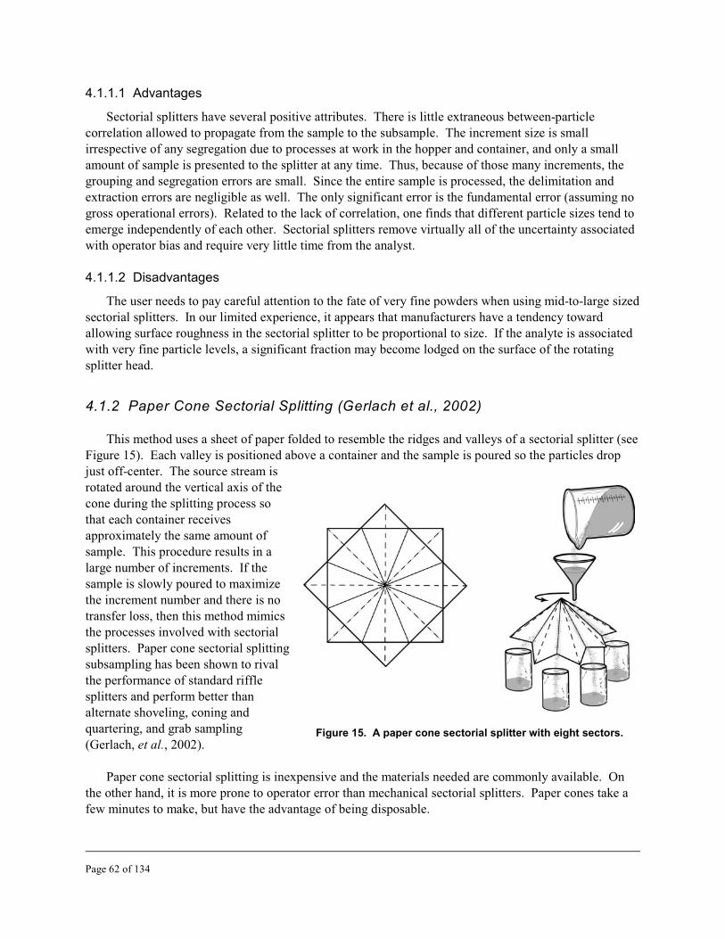
4.1.1.1 Advantages

Sectorial splitters have several positive attributes. There is little extraneous between-particle correlation allowed to propagate from the sample to the subsample. The increment size is small irrespective of any segregation due to processes at work in the hopper and container, and only a small amount of sample is presented to the splitter at any time. Thus, because of those many increments, the grouping and segregation errors are small. Since the entire sample is processed, the delimitation and extraction errors are negligible as well. The only significant error is the fundamental error (assuming no gross operational errors). Related to the lack of correlation, one finds that different particle sizes tend to emerge independently of each other. Sectorial splitters remove virtually all of the uncertainty associated with operator bias and require very little time from the analyst.

4.1.1.2 Disadvantages

The user needs to pay careful attention to the fate of very fine powders when using mid-to-large sized sectorial splitters. In our limited experience, it appears that manufacturers have a tendency toward allowing surface roughness in the sectorial splitter to be proportional to size. If the analyte is associated with very fine particle levels, a significant fraction may become lodged on the surface of the rotating splitter head.

4.1.2 Paper Cone Sectorial Splitting (Gerlach et al., 2002)

This method uses a sheet of paper folded to resemble the ridges and valleys of a sectorial splitter (see Figure 15). Each valley is positioned above a container and the sample is poured so the particles drop just off-center. The source stream is rotated around the vertical axis of the cone during the splitting process so that each container receives approximately the same amount of sample. This procedure results in a large number of increments. If the sample is slowly poured to maximize the increment number and there is no transfer loss, then this method mimics the processes involved with sectorial splitters. Paper cone sectorial splitting subsampling has been shown to rival the performance of standard riffle splitters and perform better than alternate shoveling, coning and quartering, and grab sampling Figure 15. A paper cone sectorial splitter with eight sectors. (Gerlach, et al., 2002).

Paper cone sectorial splitting is inexpensive and the materials needed are commonly available. On the other hand, it is more prone to operator error than mechanical sectorial splitters. Paper cones take a few minutes to make, but have the advantage of being disposable.

Page 62 of 134

4.1.3 Incremental Sampling (Pitard, 1993; pp. 128, 207 ff.)

An increment is a group of particles or material physically extracted from the lot (or sample) with a single operation of the sampling device. The sample (or subsample) is made from the reunion of many increments (N $ 30 increments is recommended) taken at random locations across the lot (or sample) to be represented. Incremental sampling increases the probability of sampling each location of the lot. When used with a correct sampling device, it can provide correct subsamples. However, the materialization error can inflate the uncertainty if the increments are biased due to poorly designed sampling tools. Incremental sampling relies somewhat on the skill and experience of the sampler to avoid bias and acquire a representative sample. The sampling device must allow for correct sampling. For example (see Figure 8), a scoop with a rounded bottom is not properly delimited to obtain a correct sample because it prevents one from sampling the particles at the bottom of a sample with the same probability as the particles at the top. For a correct sample, the scoop needs to have a flat bottom and parallel sides (e.g., square or rectangular).

To sample a one-dimensional lot (Pitard, 1993; p. 239), form the material into an even long pile made from many layers (the more, the better) and take at least 30 increments, each taken entirely across the pile at several equally spaced points until the sample mass, M , is acquired. Thus, if 30 increments are being s

taken to make the subsample, then the mass of each increment should be about M /30. Taking each s

increment requires a correct sampling device to remove all of the material from top to bottom in the pile. The one-dimensional pile is recommended for laboratory incremental subsampling. If the mass required for the subsample is so small that taking 30 increments is physically constraining, then fewer increments may be taken, although the error may increase with fewer increments. The relative variance due to the grouping and segregation error, sGE

2, can be made relatively small compared to the relative variance due 2to the fundamental error, sFE , by increasing the number of random increments, N. That is, for N

increments, taken with correct sampling practices (Pitard, 1993, p. 388)

2 2 2sTE2 $ sCE1 = sFE

2 + sGE # sFE2 + [s / N]FE

2 2and sTE $ sCE12 . sFE if N is made large enough. At least N = 30 increments are recommended as a rule

2 2of thumb to reduce sGE compared to s (Pitard, 1993; p. 187). Grinding the sample or using a sectorial FE

splitter may be a better option in that case.

To sample a two-dimensional lot (Pitard, 1993; p. 230), form the material into a flat pancake and take at least 30 increments at random locations using a cylindrical sampler with a constant cross section, with the sampler’s cutter perpendicular to the pile and take the increments all of the way through the pile. Two-dimensional incremental subsampling is usually not as reliable as one-dimensional incremental subsampling for the laboratory, since the material from the increment can easily fall back onto the sample surface, especially if the material is very dry.

Incremental sampling with at least 30 increments reduces the relative variance of the grouping and 2segregation error (sGE ). However, there are a few cases where this is ineffective, such as when the

number of particles with high levels of analyte is small. In this case, incremental subsampling is about as effective as taking the entire subsample at one spot. Each increment is still subject to the materialization error (ME). For incremental sampling, one must use a correct sampling device that minimizes that error

Page 63 of 134

(for example, see Figure 8). Under most circumstances, incremental sampling should allow the analyst to meet the study requirements (e.g., the DQOs).

4.1.4 Riffle Splitting (Pitard, 1993; p. 266)

A riffle splitter (sometimes known as a Jones splitter) is a mechanical device with a series of alternating chutes that deposit one-half of the sample into one discharge bin and the other half into a second bin (see Figure 16). (One should avoid any riffle splitter with an odd number of chutes.) The method is limited to free-flowing samples. Riffle splitters utilize multiple fractions (chutes), increasing the number of increments in each round, more so than methods such as coning and quartering. However, riffle splitters have much larger increments than sectorial splitters. Several varieties of riffle splitters have been developed. They are available in many sizes and some provide splitting of a sample into more than halves, such as fourths or eighths, in one operation.

Riffle splitters can perform well, but the results rely on the skill and training of the operator. The sample needs to be presented to the riffle splitter such that each chute gets a Figure 16. A riffle splitter with 20 chutes and two similar amount, and there should be no bias in collection pans.

presenting the sample to the chutes (Pitard, 1993). Schumacher et al. (1990) demonstrated that up to six passes were needed to minimize the uncertainty added with this procedure. When properly run, riffle splitters are excellent mass reduction tools (Allen and Kahn, 1970; Mullins and Hutchison, 1982; and Gerlach, et al., 2002).

While riffle splitters may have only 10 to 30 chutes, depending on the size and model, repeated passes result in each chute receiving particles from additional locations in the original sample. This causes the number of increments to be much larger than the number of chutes for the portion of the sample being processed. However, since one discards one-half of the sample in the first stage of a multiple-step mass reduction procedure, the grouping and segregation error associated with the first pass may dominate the uncertainty associated from the entire splitting process. This means that there may be very little improvement in reducing the grouping and segregation error after the first pass as the rest of the sample splitting procedure takes place.

Page 64 of 134

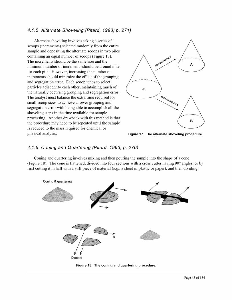
4.1.5 Alternate Shoveling (Pitard, 1993; p. 271)

Alternate shoveling involves taking a series of scoops (increments) selected randomly from the entire sample and depositing the alternate scoops in two piles containing an equal number of scoops (Figure 17). The increments should be the same size and the minimum number of increments should be around nine for each pile. However, increasing the number of increments should minimize the effect of the grouping and segregation error. Each scoop tends to select particles adjacent to each other, maintaining much of the naturally occurring grouping and segregation error. The analyst must balance the extra time required for small scoop sizes to achieve a lower grouping and segregation error with being able to accomplish all the shoveling steps in the time available for sample processing. Another drawback with this method is that the procedure may need to be repeated until the sample is reduced to the mass required for chemical or physical analysis. Figure 17. The alternate shoveling procedure.

4.1.6 Coning and Quartering (Pitard, 1993; p. 270)

Coning and quartering involves mixing and then pouring the sample into the shape of a cone (Figure 18). The cone is flattened, divided into four sections with a cross cutter having 90° angles, or by first cutting it in half with a stiff piece of material (e.g., a sheet of plastic or paper), and then dividing

Figure 18. The coning and quartering procedure.

Page 65 of 134

each half to get quarters. Alternate quarters (splits) are combined to make a subsample, and one subsample is chosen at random for any additional mass reduction until the desired subsample mass (Ms) is reached. As with alternate shoveling, this method can take considerable time to obtain a subsample.

Coning and quartering is a process that preserves particle correlations within each quadrant, and this effect is worsened by combining quarters. Essentially, one has obtained a two-increment sample containing one-half of the original mass. Thus, there is some tendency to maintain the variability due to grouping and segregation problems. In coning and quartering, there is also the difficulty of creating the initial pile so that all of the particles are randomly distributed across each quadrant. Coning and quartering is not recommended since it is a lot of effort just to reduce the grouping and segregation error by two (the number of increments, N = 2) each time that the method is performed.

4.1.7 Rolling and Quartering (Benedetti-Pichler, 1956; p. 215)

Rolling and quartering is variation on coning and quartering. The sample is placed in a conical pile on a large sheet of material with a smooth surface, such as: glazed paper, a thin plastic sheet, or rubberized cloth. The cone is then flattened and the material is mixed by rolling it back and forth. The material is returned to the center by lifting all four corners of the sheet, flattened out, and then split in half using the quartering procedure. One-half of the material is selected at random for any further mass reduction or for analysis.

The only difference between this method and coning and quartering is that some mixing takes place when the sample is rolled. This activity will cause any loosely bound clumps of particles to break apart. It may also serve to reduce some bias in the sample pile associated with pouring out the sample. Overall, there is little difference between rolling and quartering, and coning and quartering. Therefore, this method cannot be recommended, either.

4.1.8 Fractional Shoveling (Pitard, 1993; p. 272)

Fractional shoveling involves processing the sample into several subsamples. One increment (shovel-full or scoop-full) of material at a time is removed from the lot or sample (as a pile) and added in turn to form each of the subsample piles (see Figure 19). This method has characteristics very similar to alternate shoveling and the minimum number of increments should be 10 per pile. In this case, the sample is divided into several piles. The number of increments will be inversely related to the number of subsample piles and to the particle correlation level. Once the original lot or sample pile is exhausted, one of the new subsample piles is selected at random. If the subsample pile is still too large (greater than M ), then it can be reduced with another round of fractional shoveling, and the process can be repeated s

until the desired subsample mass (M ) is obtained. s

Fractional shoveling can be time-consuming for large samples. In addition, segregation effects related to density may result in trends in composition as the pile is reduced. For small samples, this may result in an increased bias between piles, as the last increment may be enriched (or depleted) compared to previous increments. If the resulting piles do not appear to be visually similar, then the sample characteristics may not be amenable to splitting by fractional shoveling.

Page 66 of 134

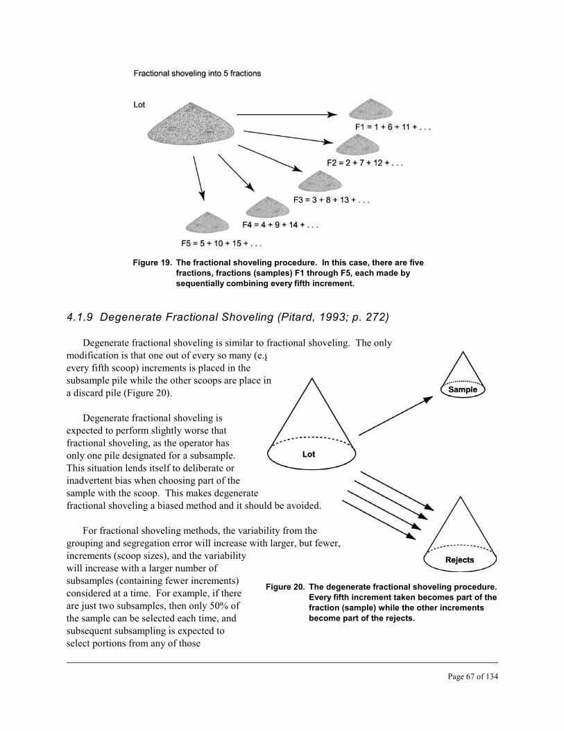
Figure 19. The fractional shoveling procedure. In this case, there are five

fractions, fractions (samples) F1 through F5, each made by

sequentially combining every fifth increment.

4.1.9 Degenerate Fractional Shoveling (Pitard, 1993; p. 272)

Degenerate fractional shoveling is similar to fractional shoveling. The only modification is that one out of every so many (e.g., every fifth scoop) increments is placed in the subsample pile while the other scoops are place in a discard pile (Figure 20).

Degenerate fractional shoveling is expected to perform slightly worse that fractional shoveling, as the operator has only one pile designated for a subsample. This situation lends itself to deliberate or inadvertent bias when choosing part of the sample with the scoop. This makes degenerate fractional shoveling a biased method and it should be avoided.

For fractional shoveling methods, the variability from the grouping and segregation error will increase with larger, but fewer, increments (scoop sizes), and the variability will increase with a larger number of subsamples (containing fewer increments) considered at a time. For example, if there

Figure 20. The degenerate fractional shoveling procedure.

Every fifth increment taken becomes part of the are just two subsamples, then only 50% of fraction (sample) while the other increments

the sample can be selected each time, and become part of the rejects.

subsequent subsampling is expected to select portions from any of those

Page 67 of 134

subsamples for final analysis. However, for 10 subsamples, or 1/10 degenerate fractions, the operator discards 90% of the sample. If a second phase of subsampling is carried out, then only 10% of the original material is available at the beginning of the second phase; thus, much of the grouping and segregation error from the first phase will remain and could influence the overall error from the remaining sample reduction steps. That is, whatever bias was introduced at the first stage will most likely influence all of the subsequent steps of the sample mass reduction process. This type of problem is similar to the one discussed for riffle splitters.

4.1.10 Table Sampler (Allen, 1997, p. 20)

A table sampler consists of an inclined surface with various triangular prisms placed to divide the sample as the surface is vibrated and the particles move from the top to the bottom (see Figure 21). Like the riffle splitter, this device splits the sample in one pass. However, the number of increments associated with this technique is small with a tendency to allow large grouping and segregation errors to remain. The device is also bulky and not readily available. This method has little to offer for recommendation. The method should suffer from operator bias in pouring the sample into the apparatus in the same manner that degrades the performance for coning and quartering, and for riffle splitting. The initial location on the table with respect to the other parts of the sample will bias certain particles toward a particular subsample. In effect, some of the initial correlation derived from the placement of the sample is maintained, and that means that some of the grouping error is maintained. Figure 21. A table sampler.

4.1.11 V-Blender (Pitard, 1993; p. 190)

V-blenders are devices for homogenizing samples (see Figure 22). However, material in a V-blender tends to segregate in the time it takes to discharge the sample, and the material will most likely segregate again as it is discharged from the bottom of the blender. Obtaining unbiased subsamples using this method would require “correct” sampling practices prior to discharging the material from the blender (this may be impossible).

Figure 22. A V-blender.

Page 68 of 134

4.1.12 Vibratory Spatula (Pitard, 1993; pp. 197, 239)

This device is sometimes used to feed material when dividing samples. Its use should be avoided. The result is more likely to enhance segregation than to reduce it. It is well known that vibrating a quantity of particles tends to enhance segregation based on size, shape, and weight.

4.1.13 Grab Sampling (Pitard, 1993; pp. 80, 205)

Grab sampling almost always involves taking the subsample off the top of the sample. One or more scoops are typically placed on a balance. The scoop, most likely an incorrectly designed sampling device, is often used to return some of the material to the sample container if the mass is larger than needed for the analytical procedure. Grab sampling does not meet the criteria of a correct sampling procedure for heterogeneous particles because it does not give each particle the same probability of being sampled. Grab sampling does absolutely nothing to reduce the sampling errors (i.e., GE, DE, and EE) that we can minimize through correct sampling techniques. If the analyte is associated with particles that have physically different characteristics, such as size, shape, or density, then a biased result is expected. If there is a tendency for the particles to segregate, then the bias and uncertainty may be very large. Grab sampling is particularly prone to generating biased results due to gravity effects and to sampler bias. Grab sampling is judgmental and nonprobabilistic, and should be avoided since it is not designed to take a representative subsample. As a sampling method, the grab sampling procedure appears to be designed to provide biased results. Grab sampling should only be considered if one has previously shown that the matrix and particle size have no significant effect upon sampling error. Even then, the analyst is at risk of reporting unreliable results if any of the samples fail to meet those assumptions. Avoid grab sampling!

4.2 Minimizing Particle and Mass Fragment Correlation

Minimizing the correlation among all of the mass fragments is similar to the criteria of sampling each mass fragment with equal probability. Several examples will show how this concept can guide the selection of sampling methods. If the selection probability is defined in units of mass fractions rather than individual particles, then the effect of large particles in any sampling scheme is now obvious. A large particle can be thought of as consisting of numerous smaller mass fraction units that behave as a single larger unit. Selecting one mass fraction that is part of the large particle causes the other smaller mass fractions to get selected too. This 100% correlation between mass fragments, whether selected into a subsample or remaining in the original matrix, results in an increased variability for any measurement. Now suppose one is preparing a subsample by fractional shoveling. The size of the scoop, or increment, is related to the level of correlation between particles that is common between the sample and the subsample. The smaller the increment, the lower the level of correlation between the particles in both the sample and the subsample. Also, the smaller the increment mass, the more random increments that can

2be taken and combined to make up the subsample mass (M ), thus, decreasing sGE . This explains why s

sectorial sampling is invariably better than fractional shoveling.

However, there is a practical limit on how small the increment can be for a correctly designed sampling device to remain correct, and it has to do with the extraction error (EE) and the size of the space of the inner walls of the sampling device. Obviously, this space must be large enough to accommodate

Page 69 of 134

the diameter of the largest fragments (d) to be sampled. Not immediately obvious, however, is that the action of the cutter moving through the sample could cause some of the fragments that should be part of the increment (that is, those fragments that have their center of gravity within the increment extended boundary) to move from the leading cutting edge making contact with those fragments to past the opposite trailing cutting edge if that space is too small. Therefore, those fragments do not become part of the sample and the quest for a fragment to have an equal chance to be part of the sample or to not be part of the sample is lost, and a sampling bias is introduced.

Pitard (1993, pp. 292 ff) gives several rules for cutter speed and inner wall sampler width. Those rules are generally summarized giving: a maximum cutter speed of 0.6 m/s; an inner wall sampler width of 3d for coarse materials (d $3 mm) and 3d + 10 mm for very fine materials, thus giving a minimum of 10 mm; and a sampler depth of at least 3d. The cutting angle should be either zero (the cutting edge is perpendicular to the extended increment) or greater than or equal to 45 degrees. Those rules may be quite constraining for the very small increments that may be needed for laboratory subsampling. If a width of less than 10 mm is used, we can only suggest (without our own empirical evidence) that the cutter speed should be much slower.

For riffle splitters, Pitard (1993, p. 302) recommends a correct riffle chute width of 2d + 5 mm. No minimum width is recommended for sectorial splitters, although an opening somewhat larger than d is obvious; however, Pitard (1993, p. 303) does recommend that the sector slope should be at least 45° for dry materials and 60° for slightly moist materials. Since true splitting methods select the splitting increments at random, the extraction bias (EE) should cancel out for those methods.

One can roughly rank the expected performance of a sample mass reduction scheme with the probability that one particle will get selected given that an adjacent particle is selected. The lower that probability (that is, the lower the correlation between the fragments), the better the expected performance. Thus, by careful review of the available options for subsampling, one should be able to rank their performance. Gerlach et al. (2002) demonstrated this concept with several common subsampling methods. Knowing the performance with one sampling method will allow the investigator to narrow or broaden the list of subsampling methods providing acceptable performance. If adequate performance levels are still not met, then reducing the fragment size may be needed.

4.3 Ranking Subsampling Methods

To rank any two methods, one must have the explicit details for the process (Mullins and Hutchinson, 1982; Gerlach et al., 2002). To compare coning and quartering to riffle splitting, for instance, one needs a few operational details. For coning and quartering, the process is briefly described as:

1) pour the sample into a single pile

2) flatten the pile

3) divide the pile into fourths

4) retain two opposing quarter fractions (i.e., only 2 increments)

5) discard the other two opposing quarter fractions (see Figure 18)

Page 70 of 134

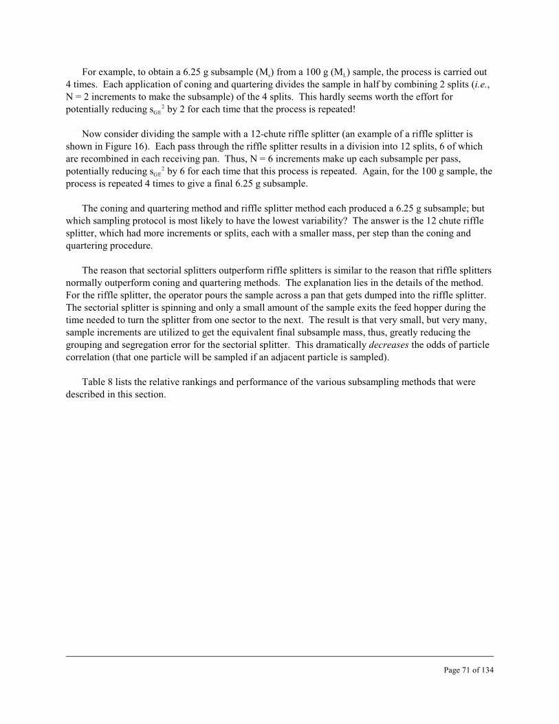
For example, to obtain a 6.25 g subsample (M ) from a 100 g (M ) sample, the process is carried out s L

4 times. Each application of coning and quartering divides the sample in half by combining 2 splits (i.e., N = 2 increments to make the subsample) of the 4 splits. This hardly seems worth the effort for potentially reducing sGE

2 by 2 for each time that the process is repeated!

Now consider dividing the sample with a 12-chute riffle splitter (an example of a riffle splitter is shown in Figure 16). Each pass through the riffle splitter results in a division into 12 splits, 6 of which are recombined in each receiving pan. Thus, N = 6 increments make up each subsample per pass,

2potentially reducing sGE by 6 for each time that this process is repeated. Again, for the 100 g sample, the process is repeated 4 times to give a final 6.25 g subsample.

The coning and quartering method and riffle splitter method each produced a 6.25 g subsample; but which sampling protocol is most likely to have the lowest variability? The answer is the 12 chute riffle splitter, which had more increments or splits, each with a smaller mass, per step than the coning and quartering procedure.

The reason that sectorial splitters outperform riffle splitters is similar to the reason that riffle splitters normally outperform coning and quartering methods. The explanation lies in the details of the method. For the riffle splitter, the operator pours the sample across a pan that gets dumped into the riffle splitter. The sectorial splitter is spinning and only a small amount of the sample exits the feed hopper during the time needed to turn the splitter from one sector to the next. The result is that very small, but very many, sample increments are utilized to get the equivalent final subsample mass, thus, greatly reducing the grouping and segregation error for the sectorial splitter. This dramatically decreases the odds of particle correlation (that one particle will be sampled if an adjacent particle is sampled).

Table 8 lists the relative rankings and performance of the various subsampling methods that were described in this section.

Page 71 of 134

Table 8.Authors’ relative rankings (from best to worst) for subsampling methods. N is the

number of increments, GE is the grouping and segregation error, N.R. means not

recommended, and N.A. means not applicable.

Typical Sensitivity to Correct Agreement

Increment Grouping & Moisture Sampling with

Method Size Segregation Content Possible FECalculated s 2 Comments

Sectorial Very Small Low Dry Yes Very Close Method of Splitter Choice

Paper Cone Sectorial Splitter

Small Low Dry Yes Close Performs Well

Incremental Sampling

Small to Medium

Moderate; Low with Many (N $30) Correct Increments

Dry to Moist

Yes, with 1-d

Pile

Close Bias Still Possible, Decreases with N and Correct Sampling

Riffle Splitting Small to Low to Dry Yes, Good to Fair Possible Loss Medium Moderate Takes Skill of Fines

Alternate Medium Low to Dry to Yes, Good to Fair Takes Time to Shoveling Moderate Moist if Careful Prepare from

a Large Lot

Fractional Medium to Moderate Dry to Yes, Fair Performance Shoveling Large Moist if Careful Tied to Lot

Mass

Table Sampler Medium Moderate to High

Dry Very Difficult; Depends on Design

Not Close High variability; N.R.

Degenerate Medium to Moderate to Dry to Yes, Unlikely Performance Fractional Large High Moist if Careful Tied to Lot Shoveling Mass; Subject

to Bias; N.R.

Rolling and Large High Dry Yes, Usually Not Highly Quartering if Careful Close Variable; NR

Coning and Large High Dry Yes, Usually Not Usually Quartering if Careful Close Biased; NR

V-Blender N.A. High Dry N.A. Very Unlikely Problems with GE; N.R.

Vibratory Spatula

Small Very High Dry No Not Close Problems with GE; NR

Grab Sampler Variable Very High Dry to Moist

No Not Close Biased and Variable; N.R.

Page 72 of 134

Section 5

Comminution (Particle Size Reduction) Methods

There are a large number of products available to reduce a sample by comminution (grinding or crushing). One must be careful to match the equipment to the sample, and to the study goals. Sample mass reduction equipment should be constructed of materials that are not of interest to the study. One should not use stainless steel grinding equipment if the analysis includes chromium. Also, some samples should not be processed with specific equipment. Pitard (1993) notes that samples with pure gold inclusions should not be reduced in a mill that pounds the sample. Since gold is very malleable, the result would be equivalent to preparing and applying gold leaf to the equipment (fashionable, but not practical!). Similarly, in one of our early studies, an attempt was made to crush a sugar sample laced with salt crystals. The result was a very fine powdered sugar, but there was no reduction in variability associated with the salt particles. The reason was that the sugar was preferentially and more easily crushed, and the much larger mass of the sugar also protected the salt particles from being broken up. If there is any doubt as to the effectiveness of a sample comminution step, several test samples should be run to verify that a lower uncertainty level was reached. Several general types of sample particle size reduction devices are listed below.

Ball Mill/Rod Mill: Ball mills come in various sizes, and can be used to convert small rock fragments to smaller mesh sizes.

Jaw Crusher: Jaw crushers can be used to reduce small rock fragments to the size of very coarse sand (3 cm to 2 mm).

Disk Mill: Disk mills can reduce particle size diameters from several mm to less than 0.5 mm.

Ring and Puck Mill: A ring and puck mill (also known as a shatterbox or a rotary mill) uses an orbital motion to force a circular center piece of steel (reminiscent of a hockey puck) against an outer steel ring. Particles are crushed between the edges of the ring and puck, and between the bottom of the pan and the puck. The end result is a fine powder (< 0.05 mm).

Vibratory Ball Mill, Planetary Ball Mill, and Ring Mill: These are all examples of completely enclosed techniques appropriate for small sample sizes. One must be careful to select (ball or ring) materials which are not made up of, or will not interfere with, the analyte of interest.

Mixer Mill: A mixer mill can be used to reduce small (< 20 g) samples into a fine powder. The sample is placed in a capsule with a ball or rod. The capsule and ball or rod are all made of high strength materials. The filled capsule is shaken at a high speed to convert the sample into a powder. Mixer mills are used instead of ring and puck mills to limit the effect of contamination when the sample mass is small.

Page 73 of 134

Page 74 of 134

Section 6

Sample Characterization and Assessment

Every environmental site is unique and each matrix will have different characteristics. The attributes of the matrix must be known before the sampling requirements can be identified. A site sampling design that results in an accurate summary of environmental conditions relies on knowing the sample characteristics across a site. Likewise, someone taking a subsample from a heterogenous particulate sample sent to a laboratory needs to evaluate the characteristics of the entire sample, not just the top layer.

Frequently, the analyte of interest is highly concentrated in the fine particulate fraction of the sample. This can result in fractionation and a bias if correct sampling techniques are not used since the small particles can drop to the bottom of a sample no matter how much the sample is shaken.

Information about the particles containing the analyte of interest is particularly useful in assessing whether a proposed sampling practice is acceptable. Is the analyte concentrated in several particle types or in just one type of particle? Are there particles highly concentrated in the analyte resulting in a density effect? Do the analyte, or analyte-rich, particles have different densities, shapes, texture, or other features that distinguish them from the other particles in the sample? How does the size distribution of analyte particles compare to the size distribution for the entire sample?

6.1 Identifying Important Sample Characteristics

Almost every characteristic of a particle is directly or indirectly related to some factor affecting sampling uncertainty. The directly related factors are considered in Gy sampling theory. Indirect, or proxy, factors are features that are correlated to the actual factors. For instance, the color or hue of a particle may be related to the amount of contaminant, and the texture might be related to density. While Gy sampling theory was developed with consideration of the contaminant levels, there has been no mention of color or texture. However, when sample assessment is the goal, any direct or indirect indicator of the nature and complexity of the sample should be used to formulate decisions about how to process the sample. The following list includes examples of both direct and proxy factors related to sampling uncertainty.

Color (hue and intensity) Hardness Mottling Structure

Composition Mass (weight) Opacity Texture

Concentration Mineral type Porosity Variegation pattern (stripes,

Density Moisture (and other liquid) Shape streaks, or speckles)

Friability content Size

Page 75 of 134

The analyst should consider all of those factors in assessing the sample. The above descriptors refer to the properties of individual particles. A description of the sample also includes information related to groups of particles with common characteristics; for instance, the size distribution of the analyte­containing particles. A complete description with respect to the possible factors could result in a large multivariate data set.

The ways to identify the sample characteristics include visual inspection, and chemical and physical analysis. These are not mutually exclusive, though many characteristics that are not subject to visual assessment are only known through measurement and analysis.

6.2 Visual Characteristics

Sometimes a reasonable sampling design can be proposed once the visual characteristics are known. Many particle characteristics can be determined through careful inspection. A magnifying glass or a microscope may be useful in identifying whether or not multiple particle types are present. Visual assessments are quick, inexpensive, and provide sufficient information for many sampling decisions. A visual assessment may reveal if the sample is composed of different types of particles by looking at their color, shape, size, texture, and other distinguishing features (be sure to look at different parts of the sample, or at randomly selected increments, because of grouping and segregation effects). The features that one is most interested in are the features important to the Gy sampling theory.

6.2.1 Analyte Particles: Color, Texture, Shape, and Number

Color, texture, and shape are distinctive visual clues related to important characteristics in Gy sampling theory. While these factors are not useful in generating quantified uncertainty estimates, they could be excellent proxies for many sample properties that are directly related to uncertainty. Different source materials usually have distinctive features. They also tend to have individual size distributions.

The most important visual feature is one that distinguishes analyte containing particles from non­analyte particles. Identifying these features might be difficult because the sample may contain many particle types and several analyses may be required to determine if they are associated with the analyte of interest (such as a hazardous material at a site). However, sometimes prior information about the lot (e.g., a site) provides the desired information. If so, then one should consider whether or not the expected number of analyte particles is large enough to approximate their distribution with normal distribution statistics.

A rough rule of thumb is that an average of 6 or more particles per sample is required before normal distribution statistics can make a reasonable approximation. If one is splitting a sample, then the minimum number of each type of particle in the parent sample should be more than 6 times the number of possible subsamples because the sample splitting process may not uniformly distribute the particles of interest among the subsamples. Some subsamples may get more than 6 particles and some will get less than 6. We suggest a factor of 10 times the number of subsamples so that most of the subsamples will have at least 6 analyte particles. For example, for a single pass of a parent sample through a riffle splitter, the number of possible subsamples is 2 and, therefore, the number of contaminant particles in the parent sample should be at least 20 (to approximate a normal-shaped distribution so that the expected

Page 76 of 134

proportionate number of contaminant particles in the subsample is the same as the proportion of contaminant particles in the parent sample).

6.2.2 Unique or Special Features

Some samples will contain particles with rare or unusual characteristics. These particles may be related directly or indirectly to the amount of contamination in the sample. The analyst should note any distinguishing characteristics for the different component particles in the sample as this may prove to be valuable information at a later date. If there are any visually distinctive features, then they should be present in all of the sample splits with the same proportion as the original sample. If one can determine a difference visually, then it is likely that there will be a significant measured difference between the subsample and original sample.

A sample may also contain unexpected material (e.g., gum wrapper, bottle top, shotgun shell casing, etc.). The sample processing plan should address how the sample should be treated when unexpected components are present. For instance, if soils are being sampled, there should be a standard protocol with respect to dealing with organic objects such as large bark chips or root fragments. If the study design allows objects larger than the particle size associated with acceptable uncertainty, then the sample must be modified prior to subsampling.

6.2.3 Density

Density is the principal cause of segregation of different particle types and is often associated with visual cues, such as color, shape, and texture. If a particle type has a significant density difference and another distinctive visual characteristic, then the analyst will be able to make a cursory check that fractionation is affecting the subsampling process. Density differences are usually inferred from visual observation, with occasional measurement confirmation. If one observes obvious density differences, then subsampling methods should be chosen that are least affected by it.

6.3 Moisture Content and Thermally Sensitive Materials

Wet samples are often air- or oven-dried to reduce the moisture content prior to any sample modification. Under such conditions, volatile, and perhaps semi-volatile, components cannot be determined (those components may also escape) when particle size reduction is required. If the sample is dry and flows freely, then the analyst should continue the assessment process by evaluating the particle size.

Thermally sensitive contaminants require a sampling design compatible with the compounds of interest. If wet samples are anticipated, then the design should identify whether the samples are to be processed wet or to be dried first. This guidance adequately addresses only dry samples.

Page 77 of 134

If the sample is wet or does not flow freely due to the presence of moisture, then one must decide to either:

< Dry the sample, restore the particle nature of the sample (gently roll or physically break up the sample without changing the particle distribution), and continue

or

< Take a subsample for analysis, then dry it

The first decision is preferred if one is trying to characterize the analyte proportion (concentration) in the original sample by analyzing a subsample. The second decision is preferred if one is splitting a sample to get representative subsamples, including a representative moisture content, since moisture content can also vary over the lot or sample to be represented. In any case, the analytical subsample must mimic the particle size distribution of the sample. In addition to one-dimensional incremental sampling, two-dimensional incremental sampling may also be appropriate for moist samples (see subsection “4.1.3 Incremental Sampling,” page 63).

It is assumed that there is sufficient water in the sample to cause the particles to adhere to each other but not to flow. Moisture could affect a number of mechanisms involved with particulate heterogeneity, such as the distribution heterogeneity (grouping and segregation effects). Also, note that wet samples can cause problems with comminution devices; hence, it may be difficult to reduce sFE

2 by comminution. The moisture content may also interfere with the analysis.

Drying is an alteration of the chemical and physical composition of the sample; therefore, drying is considered a materialization error; specifically a preparation error. Obviously, drying will affect the estimation of the proportion of the analyte in the analytical subsample as compared to the sample, and this can greatly affect decisions. Therefore, it is imperative that the moisture content is documented. The moisture content must be accounted for in drying operations, which should be well documented (as should be the calculations of the results). The analytical results must be descriptive about the moisture content, such as “80 ppm Pb, dry weight sample” or “7 ppm Cd, 20% water by weight in sample.” It is important that the moisture content does not change between the sampling step and the weighing step and the analysis step (protect samples with a desiccator). Determining the moisture content can be tricky with respect to sampling and the reader is directed to read the sections given by Pitard (1993), “the simultaneous drying method” (pp. 322-323) and “the method of the single sample” (pp. 323-326).

6.4 Particle Size, Classification, and Screening Decisions

Sieving a sample provides information about particle size distributions, and the analysis of various fractions can aid in determining whether or not analyte levels are dependent on particle size. If a sample matrix does have unique particle types, then the general mix of particles in the subsample should be similar to the mixture seen in the original sample. However, this is only a check for gross differences, and analytical measurements are required to determine whether the subsampling procedure is performing adequately.

Particle size is a key decision characteristic for the application of Gy sampling theory. The size of the largest particles is a critical factor in determining the expected uncertainty. The long axis particle

Page 78 of 134

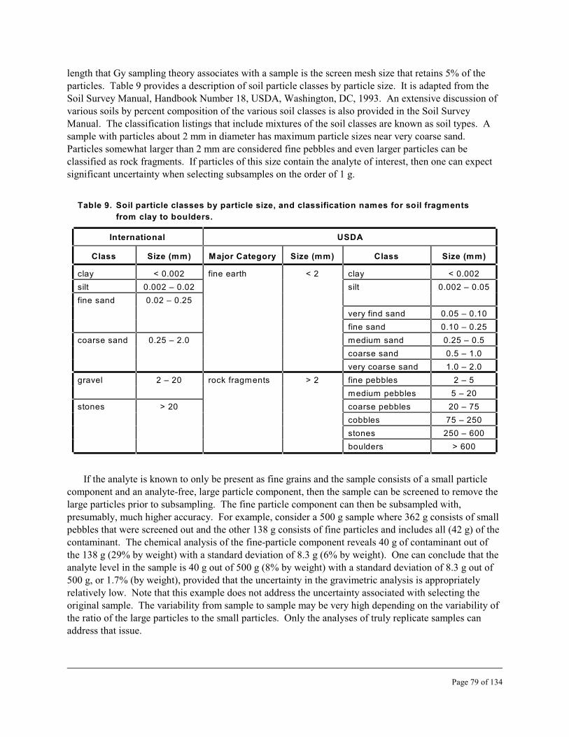
length that Gy sampling theory associates with a sample is the screen mesh size that retains 5% of the particles. Table 9 provides a description of soil particle classes by particle size. It is adapted from the Soil Survey Manual, Handbook Number 18, USDA, Washington, DC, 1993. An extensive discussion of various soils by percent composition of the various soil classes is also provided in the Soil Survey Manual. The classification listings that include mixtures of the soil classes are known as soil types. A sample with particles about 2 mm in diameter has maximum particle sizes near very coarse sand. Particles somewhat larger than 2 mm are considered fine pebbles and even larger particles can be classified as rock fragments. If particles of this size contain the analyte of interest, then one can expect significant uncertainty when selecting subsamples on the order of 1 g.

Table 9. Soil particle classes by particle size, and classification names for soil fragments

from clay to boulders.

International USDA

Class Size (mm) Major Category Size (mm) Class Size (mm)

clay < 0.002 fine earth < 2 clay < 0.002

silt 0.002 – 0.02 silt 0.002 – 0.05

fine sand 0.02 – 0.25

very find sand 0.05 – 0.10

fine sand 0.10 – 0.25

coarse sand 0.25 – 2.0 medium sand 0.25 – 0.5

coarse sand 0.5 – 1.0

very coarse sand 1.0 – 2.0

gravel 2 – 20 rock fragments > 2 fine pebbles 2 – 5

medium pebbles 5 – 20

stones > 20 coarse pebbles 20 – 75

cobbles 75 – 250

stones 250 – 600

boulders > 600

If the analyte is known to only be present as fine grains and the sample consists of a small particle component and an analyte-free, large particle component, then the sample can be screened to remove the large particles prior to subsampling. The fine particle component can then be subsampled with, presumably, much higher accuracy. For example, consider a 500 g sample where 362 g consists of small pebbles that were screened out and the other 138 g consists of fine particles and includes all (42 g) of the contaminant. The chemical analysis of the fine-particle component reveals 40 g of contaminant out of the 138 g (29% by weight) with a standard deviation of 8.3 g (6% by weight). One can conclude that the analyte level in the sample is 40 g out of 500 g (8% by weight) with a standard deviation of 8.3 g out of 500 g, or 1.7% (by weight), provided that the uncertainty in the gravimetric analysis is appropriately relatively low. Note that this example does not address the uncertainty associated with selecting the original sample. The variability from sample to sample may be very high depending on the variability of the ratio of the large particles to the small particles. Only the analyses of truly replicate samples can address that issue.

Page 79 of 134

6.5 Concentration Distribution

A variety of uncertainty components are associated with the distribution of the analyte among the particles. Identifying the analyte proportion (or concentration levels) versus the particle size distribution would be very valuable; however, this is difficult to determine visually or experimentally. Occasionally, one can identify the presence of a few large or highly concentrated particles, which suggests that a nugget effect may be expected (a nugget effect includes the random variance in estimating the parameters: the mean proportion of the contaminant within a sampling unit, the mean mass of a sampling unit, and the small scale heterogeneity within a sampling unit (Pitard, 1993, pp. 109 ff.). If analyte particles are identifiable and rare (such as an occasional lead shot in a soil matrix), then the analysis results may be distributed as a Poisson distribution or some similar, highly skewed probability distribution, and the level of uncertainty reported for any analysis should include this possibility.

If large inert particles (e.g., pebbles and rocks) containing little or no analyte, then the variability of any subsample analysis will increase. Even if all of the analyte is present as a fine powder, the sampling variability may increase dramatically due only to the uncertainty associated with the larger inert components.

6.6 Comminution (Grinding and Crushing)

If the sample consists of small enough particles to achieve an acceptable error, then no particle size changes are needed. Otherwise, the size of the particles needs to be reduced, increasing the number of particles and reducing the relative variance of the fundamental error. If grinding is not an acceptable option, then the mass of the subsample, M , should be increased. s

Quick and rough estimates of the sample mass, M , required for the corresponding minimum s

particulate sizes to obtain a CV (%RSD) of 15% (i.e., a relative variance of 0.0225) for sFE are summarized in Table 10 (from ASTM D 6051; see also Ramsey et al., 1989; and Pitard, 1993). Note that about a factor of 10 in mass is associated with about a factor of 2 in particle size. The dominant cause of this relationship is that the required mass is proportional to the cube of the particle diameter. For most situations, this means that particle size is the key consideration. Screening the sample (or a representative subsample) to identify the particle size distribution is a quick way to estimate whether particle size reduction is needed. For more accurate estimates of the required minimum sample mass, the equation used for estimating the relative variance for the fundamental error should be used; a sampling strategy based on the sampling nomograph should also prove useful.

Page 80 of 134

Table 10. The minimum sample mass, M , s

and the maximum particle size, d,

for sFE # 15% (density = 2.5,

analyte weight proportion = 0.05).

sMinimum M [g] Maximum d [cm]

5 0.170

50 0.37

100 0.46

500 0.79

1000 1.0

5000 1.7

6.6.1 Caveats

Size reduction strategies, such as grinding, are inappropriate when the analyte is soft and not amenable to comminution, or if the analysis is intended to determine only the exposed or easily recoverable component. For example, only the easily extractable metals might be of interest since components imbedded within the sample matrix would not be considered hazardous.

Page 81 of 134

Page 82 of 134

Section 7

Proposed Strategies

A number of strategies and lists of sampling criteria related to the subsampling of particulate materials have been published (Pitard, 1993; Kern et al., 1997; and Mishalanie and Ramsey, 1999). Please refer to those references and the text presented in this guidance for details. The proposed strategies presented here build on previous suggestions, but are more comprehensive. The extra features are the result of realizing that sampling particulate material is a multifaceted problem that cannot be easily summarized. The reader is reminded that the following is only guidance and the best strategy will likely be some variation on what is presented here. The best strategies will only be developed when the analyst has an understanding of the fundamental principles of the sampling theory for particulate materials and an actual sample to observe and test. Although common strategies can be developed and used as a general guidance, sampling plans are not generic and a sampling plan should be developed for each unique case.

The goal of our sampling strategy is to reduce data uncertainty by selecting a representative analytical subsample (representative of the laboratory sample). The analytical subsample is that mass which undergoes analysis. A representative sample can only be attained through correct sampling practices. Recall (refer to the text or the glossary) that the total sampling error is

TE = FE + GE + CE + CE + DE + EE + PE 2 3

If correct sampling practices are used, then the terms, GE, DE, EE, and PE are minimized; that is, GE + DE + EE + PE . 0. Assuming that CE + CE = 0 for laboratory subsampling, and if correct sampling 2 3

practices are used, then the total sampling error becomes

This is the minimum sampling error due simply to the nature of the material being sampled (the constitution heterogeneity) and represents a goal of Gy’s correct sampling practices.

The mean of the total sampling error then becomes the mean of the fundamental error under the conditions of correct sampling practices and negligible effects from CE and CE , and is expected to be 2 3

negligible; that is,

Page 83 of 134

The relative variance of the total sampling error is

2 2 2sTE2 = sFE

2 + sGE + sCE22 + sCE3 + sDE

2 + sEE + sPE2.

2 2 2 2 2If correct sampling practices are used, then the terms sGE , sDE , s , and s are minimized; that is, s EE PE GE 2 2 2+ sDE

2 + sEE2 + sPE . 0. Assuming that sCE2 + sCE3 = 0 for laboratory subsampling, and if correct

sampling practices are used, then the relative variance of the total sampling error becomes

2s = sFE2

TE

This is the minimum sampling relative variance due simply to the nature of the material being sampled (the constitution heterogeneity) and is the basis for developing a representative sampling strategy using Gy’s correct sampling practices.

The degree of representativeness, rTE2, is given by

2rTE2 = m TE

2 + sTE

2 2where rTE is the mean square of the total sampling error, m is the square of the mean of the total TE 2sampling error, and sTE is the relative variance of the total sampling error. A sample is representative

when

2rTE2 # roTE

where roTE2 is a specified and quantitative measure of a representative sample (the smaller this number,

the more representative is the sample); that is, it is a level of representativeness regarded as acceptable as defined by the study objectives (e.g., data quality objectives, DQOs) and the sampling plan.

We can estimate how representative our analytical subsample is of the laboratory sample by developing a strategy such that the bias is negligible (mTE

2 = 0) and the “controllable” relative variances are minimized when the sampling practices are perfectly correct (that is, when GE = DE = EE = PE = 0).

2 2 2It is desirable to keep s # soTE , where s is a level of the relative variance of the total sampling error TE oTE 2 2within user specifications. If sampling practices are perfectly correct (that is, s = sDE

2 = sEE = sPE2 = GE

20), then s = sFE2 (the relative variance of the fundamental error). Thus, if correct sampling practices TE

s

are applied and all of those “controllable” errors are minimized, then a representative sample could be characterized by keeping the relative variance of the fundamental error below a specified level, sFE

2 #

oFE2. Under such conditions,

2rTE2 . sFE

2 # soFE . roTE2

This equation will serve as the basis of our sampling strategy to obtain a representative subsample for analysis. This is fortuitous for our sample planning purposes, and for formulating our study objectives

2(e.g., DQOs), since s is the only error that can be calculated, based on the physical and chemical FE

properties of the particulate material, a priori; that is, before sampling even takes place! Thus, the user now has a logical approach to specifying the tolerable amounts of bias and variability as set by the study objective (e.g., DQOs), and a basis for a sampling strategy.

Page 84 of 134

The above discussion on the theory behind developing a strategy to get a representative analytical subsample may seem like a lot to take in, and the ensuing discussion on developing a practical sampling strategy may seem like too much effort just to analyze a small amount of material. When one is in a hurry and has a large case load, it may seem downright threatening and overwhelming. But, remember that the seemingly simple task of taking a small amount of material out of a laboratory sample bottle could possibly be the largest source of error in the whole measurement process. Not taking a representative subsample could produce meaningless results, which is at the very least a waste of resources, and at the very most, could lead to disastrous decisions and consequences.

Sampling is one of those endeavors that you “get what you pay for,” at least in terms of effort. But the effort is not necessarily that much. It pays to have a basic understanding of the theory. Become familiar with what causes the different sampling errors and how to minimize them through correct sampling practices. Be able to specify what constitutes a representative subsample. Know what your sampling tools are capable of doing and if they can correctly select an increment. Do a sample characterization (at least a visual inspection) first. At a minimum, always have study objectives and a

2 2sampling plan for each particular case. One should determine the maximum s and sAE that will be FE

tolerated, and the final M for analysis. If possible, a team approach should be taken for developing the s

study objectives and the sampling plan. Historical data or previous studies should help here. Be sure to record the entire process.

The generic strategy proposed below is meant to be fairly comprehensive for developing plans for most situations (see the text for some exceptions; also, see Pitard, 1993). If the generic strategy seems a bit too overwhelming for the intended purposes, then at least try to use correct sampling practices and correct sampling devices the best that you can under your circumstances. Try to take as many random increments as you can (a sectorial splitter is a good tool for this). If you can only take a few, say five, increments rather than the recommended 30, then you are still better off than taking a grab sample “off the top” from the sample bottle. And now, you are at least aware of the consequences of only reducing

2sGE2 by N = 5 increments relative to s ; recall that FE

sGE2 . sFE

2 / N

and

2 2 2sTE2 $ sCE1 # sFE + [s / N]. FE

2 2Thus, sTE $ sCE12 . sFE if N is made large enough. (At least N = 30 increments are recommended as a

2 2rule of thumb to reduce sGE compared to s (Pitard, 1993; p. 187).) Grinding the sample to a fine FE

powder followed by taking many increments may be another “quick” alternative. Also, the sampling nomograph provides an effective visual aide for quickly developing a subsampling plan.

7.1 The Importance of Historical and Preliminary Information

If practical, preliminary trial samples, analyzed in advance of the study, may prove useful so that the study designers can identify an appropriate subsampling method that meets the study DQOs.

Page 85 of 134

To determine which subsampling methods are important, an assessment of the possible sampling errors should be made and compared to the study DQOs. Based on the sample matrix, the analytical procedure, and the study DQOs, one can assess the relative importance of the sampling methods following the guidance in this document. The test samples may be analyzed using any sampling technique shown to meet the study criteria in terms of relative error. Several representative subsamples should be analyzed to determine if variability is an issue. With data from six or more representative subsamples, one can compare the variability and the recovery between sampling techniques. Variability is much more important at this stage.

If the variability is acceptable, then no particle size reduction may be necessary. If not, then a different spitting method is needed or the sample characteristics must be altered before subsampling. Unfortunately, some samples may have characteristics that are difficult to detect, such as rare, but high level, contamination patterns. The analysis of test sample results is merely an alternate way of identifying conditions in the particulate matrix. If all of the particles are fairly homogeneous in the analyte levels, then the variance due to the particle size distribution should be small, and low uncertainties should be expected. The same particle size distribution may give large uncertainties if the analyte is confined to one of many particle types in the sample. This demonstrates the need for prior information concerning the sampling site. Information about the site provides crucial information needed to efficiently evaluate possible sampling strategies.

If several representative laboratory samples are present, then one can identify the minimum errors expected from simple preparation and subsampling efforts. These can be compared to the study requirements to determine if more intensive processing is desirable. Alternatively, one can evaluate individual characteristics of the sample. For instance, one might determine if the analyte is confined to the fine particulate fraction. Perhaps it is possible to reduce the mass by merely screening the sample as part of an initial processing step.

7.2 A Generic Strategy to Formulate an Analytical Subsampling Plan

The initial assumption is that the analyst must obtain a representative laboratory analytical subsample from a laboratory sample composed of a heterogeneous collection of particles. The laboratory analytical subsample is the subsample that undergoes laboratory analysis to estimate the analyte concentration, a . s

The laboratory sample is the sample (and, in this case, the lot) received by the laboratory containing an analyte concentration, a (which is estimated by a ). L s

At this point, we may not know how the sample received by the laboratory was collected. For instance, the laboratory sample may not have been selected using correct sampling methods and may not be representative of the original lot (e.g., a hazardous waste site). Therefore, our attempt in the laboratory is to select the analytical subsample so that it is representative of the laboratory sample that was received and we should not be tempted to extrapolate claims beyond the laboratory sample (e.g., about the site) for which we may have no knowledge or control.

The particles are of various sizes, shapes, and composition, and the analyst may not know which particle(s) is important in terms of the analyte of interest. The lack of initial information can be a limiting factor in being able to identify the best strategy to use when producing a laboratory analytical

Page 86 of 134

subsampling plan. The following steps allow one to gather information and develop strategies for preparing representative laboratory analytical subsamples that meet a study’s uncertainty requirements.

1. Examine the sample as outlined in the section on “Sample Characterization and Assessment.”

2. This step provides a bound on the variability contributed by sampling and other factors in the measurement process. The following should be identified up front in the planning stage when determining the study requirements (e.g., DQOs):

< Determine the acceptable level of error for the laboratory analytical subsampling step; that is, determine the acceptable level of the bias for the total sampling error, m0TE, and the

2relative variance for the total sampling error, s0TE . Determine the degree of acceptable 2 2 2representativeness, r , given by r0TE = m0TE + s0TE

2.0TE

< Ascertain the error limits for the study; that is, determine the acceptable level of the bias for the overall error, mOE, and the relative variance of the overall error, which is a linear combination of the relative variance of the total sampling error and the relative variance of

2 2the analytical error (which should already be known): s = sTE2 + sAE .OE

< Try to identify any other error contributions from other steps in the measurement process.

3. Determine if the sample has any unique features that require a special treatment prior to subsampling. Those features and treatments, and how to correct for them, should be identified up front in the planning stage when determining the study requirements (e.g., DQOs). For example:

< If the sample has a high moisture content, then it may need to be dried.

< Unexpected items (e.g., twigs) may need to be removed.

< If large inert (no contaminant) particles are present, then they may need to be removed or reduced in size. In that case, the new diameter of the largest remaining particles becomes the

2diameter, d, used in the equation to estimate sFE .

4. Estimate the laboratory sample analyte concentration level, a , and (if possible, but not L

necessary) try to determine how the analyte is distributed in the sample.

< Knowing the sample analyte concentration is of course necessary for the laboratory analysis (e.g., choosing the correct analytical method and the range of calibration standards); however, it can also help in refining the estimates of the constant terms used in the relative variance for the fundamental error equation. Knowing if the analyte (contaminant) is expected throughout the sample or is present as isolated particles provides information relevant to subsampling methods and decisions about reducing the particle size. Try to determine if the analyte is distributed across most of the particles or if the analyte is distributed in a highly heterogeneous manner, occurring at high levels in a few particles and at low levels in the other particles.

< If the analyte of interest is confined to a limited range of particle sizes or types, then (if consistent with the study requirements identified in step 3) remove and analyze only the

Page 87 of 134

portion of the sample containing the analyte of interest. Be sure to record all of the actions and the weights of the fractions.

< Disadvantages of removing and analyzing only the active particle size fractions: Requires screening each sample to identify the size fraction containing the analyte of interest. Requires sample separation by size fraction. Hence the sample must be fairly dry prior to separation, possible affecting volatile and liquid compounds.

< Advantages of removing and analyzing only the active particle size fractions: The analysis is targeted only at the contaminated fractions, limiting the sample amount required for processing.

< When it is known that the target compound is not present in the large particles, screen out all of the material (weigh this material) larger than the analyte particles size level. The remaining sample is processed with the standard protocol and the reported concentration is corrected for the amount of matrix that was removed.

< Disadvantages of removing the larger inert material: Volatile compounds may be lost or diminished in concentration during processing. A sample large enough to meet the uncertainty requirements for both the screened material and the screened out material must be available.

< Advantages of removing the larger inert material: The number of required sample analyses is minimized.

5. Estimate the size of the largest particles (d).

< Using the diameter of the largest particles in the relative variance for the fundamental error 2equation gives the most conservative estimate of sFE based on a given diameter. The

equation for the relative variance for the fundamental error, sFE2, is more dependent on

particle size (because it is cubed) than any other factor. A very rough rule of thumb is that if the diameter of the largest particles is less than around 2 mm, then the sample variability is likely to be small. Samples with larger particles may require a size reduction step.

6. Estimate the density of the analyte, , and the density of the gangue (matrix), .

7. Estimate the constant terms (c, l, f, and g) in the equation for the relative variance for the fundamental error.

< The constant terms, l (the liberation factor), f (the shape factor), and g (the granulometric factor), can be estimated by measurements (see this text and Pitard, 1993) or by observations and using Tables 4, 5, and 6.

< The mineralogical factor, c, is given by

Page 88 of 134

where a is the decimal proportion [unitless] of the analyte in the sample, 8 is the density of L M 3 3particles containing the analyte [g/cm ], and 8 is the density of the gangue [in g/cm ]g

28. Estimate the relative variance of the fundamental error (s ) based on the required subsample FE

mass (M ) for the laboratory analysis. s

< If one knows the particle size, d, the required laboratory analytical subsample mass, M , and s

the constant terms in the equation for the relative variance for the fundamental error, then an estimate of the relative variance of the fundamental error, sFE

2, can be made:

where M is the sample weight [g], M is the mass of the lot [g], c is the mineralogical (or S L-3composition) factor [g cm ], l is the dimensionless liberation factor, f is the dimensionless

particle shape factor, g is the dimensionless particle size range (or granulometric) factor, d is -3the nominal size of the particles [cm], C = cflg is the sampling constant [g cm ], and IH is L

the constant factor of constitution heterogeneity (also called the invariant heterogeneity).

< If the laboratory sample (the lot) is large compared to the analytical subsample, that is, M L

>> M , then the term, 1/M , is negligible and the relative variance of the fundamental error s L

is:

< Those constant terms can be estimated by measurement or by observation, and by using tables (see Tables 4, 5, and 6). A quick and very rough estimate of the relative variance of the fundamental error can be made using some “typical” values for the constant terms:

s

< Estimating the relative variance of the fundamental error provides a quantitative value that can be reviewed in light of the study’s uncertainty requirements (e.g., DQOs). This predicted sFE

2 should be well within the bounds of the minimum uncertainty identified from the study objectives (e.g., the DQOs) and step 2 (vide supra). Remember that this predicted

FE2 is the minimum sampling error possible and there most likely will be other contributions

2 2(like s ) to the relative variance of the overall error (s ). Even when correct sampling AE OE

practices are followed, small amounts of concentrated nuggets can inflate the total sampling variance, and the relative variances due to the other sampling errors may still make a

2 2 2 2 2 2contribution to sOE . Recall that sOE = sFE2 + sGE + sCE2

2 + sCE3 + sDE2 + sEE + sPE

2 + sAE . Take advantage of this step since the relative variance of the fundamental error is the only sampling error that can be estimated prior to subsampling.

9. If the variance of the fundamental error (s 2) based on the required subsample mass (M ) for FE s

laboratory analysis is not well within the bounds of the minimum uncertainty identified from

Page 89 of 134

the study objectives and step 2, then calculate the laboratory subsample mass (Ms) needed to 2achieve the desired sFE .

< Reducing the variance of the fundamental error (s 2) can be achieved by increasing the FE

laboratory subsample mass (M ); however, this increased subsample mass must be s

compatible with the analytical method.

< Disadvantages of increasing the laboratory subsample mass (M ): It is expensive and s

cumbersome to process large samples. The extraction facilities may not be large enough.

< Advantages increasing the laboratory subsample mass (M ): Besides reducing the s

fundamental error, this action may be effective if the analytical process can be easily adapted to large sample masses. For instance, if the analyte can be extracted prior to analysis, the issue of subsampling variability disappears at the laboratory stage.

10. Consider particle size reduction (comminution - see text) if the required laboratory subsample mass (M ) is too large. s

< Use the sampling nomograph (see text) to develop a subsampling strategy with the fewest comminution (grinding or crushing methods) steps to obtain the laboratory subsample mass

2(M ) that meets the desired sFE . Be sure to allow for the propagation of error if there is more s

than one mass reduction (subsampling) step (see the “Hypothetical Example” and Figure 13 in the text under the “Sampling Nomograph” section). The size reduction (comminution) steps are designed to reduce uncertainty due to particle size and variable composition effects.

< Disadvantages of comminution: Comminution is not appropriate if volatile compounds are of interest, as a significant bias would be expected. Comminution is not appropriate for wet or oily samples, or when the analyte is a soft metal (which is not amenable to grinding). For large samples, the effort may be correspondingly large.

< Advantages of comminution: Besides reducing the fundamental error, grinding can also help to reduce the grouping and segregation error. For small samples, the cost-to-benefit ratio may be relatively low.

11. Collect (select) the laboratory analytical subsample using correct sampling equipment (see text) and correct sampling practices (see text).

< Correct sampling means to minimize the effects of all of the sampling errors that we have control over through our sampling techniques. This includes all of the sampling errors except for the relative variance of the fundamental error (sFE

2), which can only be reduced by increasing the sample mass, M , or by reducing the particle size, d, though comminution s

(crushing or grinding). Consider either incremental subsampling or splitting subsampling methods (see text).

< For incremental or splitting subsampling, the relative variance of the grouping and segregation error (sGE

2) can be reduced by taking at least 30 random increments to make up the subsample. To correctly select an increment with respect to the increment delimitation error (DE), the sides of the sampling device should be parallel with a flat bottom (e.g., a scoop) for a one-dimensional (that is, one long dimension) pile or the sampling device should

Page 90 of 134

have a constant diameter (e.g., a cylinder) for a two-dimensional (that is, two long dimensions) surface or cake, and the sampling device should go completely through the pile or surface and at a slow, even rate. A rule of thumb for correctly collecting an increment with respect to the increment extraction error (EE) is that the inside diameter of the sampling device should be at least 3 times the diameter of the largest particle. Splitting methods are not generally affected by DE or EE if the splitters have a good design and good technique is used. Some splitting subsampling methods are recommended somewhat over incremental methods, with the sectorial splitter being the method of choice. Last, but not least, the preparation error (PE) is reduced through common sense, honesty, and awareness.

7.3 An Example Quick Estimate Protocol

Any large rocks in a sample should be broken up into fragments no larger than about 2 to 3 cm in diameter. For most samples, this is easily accomplished with a hammer or small sledge hammer. Then, the samples with fragments up to about 3 cm in diameter should be crushed to the level of very coarse sand, with grain sizes about 2 mm in diameter. This step requires a mechanical crusher. The particle size can be reduced again in one or two stages:

Two stage process

The entire sample can be reduced in size from very coarse sand to a medium or fine sand with a disk mill. A subsample of about 100 g (20 to 200 g range limit) is then taken with a riffle or sectorial splitter. The subsample is then ground in a rotary ring and puck mill to a fine powder (< 0.05 mm diameter). The two-stage process has the advantage of processing the entire sample until subsampling just before the final particle size reduction stage.

One stage process

A subsample of about 100 g is taken with a riffle or sectorial splitter without having gone through the disk mill. The fundamental error is larger for this method because it affects the variability of the subsampling step.

Page 91 of 134

Page 92 of 134

Section 8

Case Studies

8.1 Case Study: Increment Subsampling and Sectorial Splitting

Subsampling

A simple example illustrating the difficulty associated with particle sampling is presented by Gerlach et al., (2002). Eight, 5 g subsamples from a 40 g mixture consisting of 0.2 g NaCl and 39.8 g of screened (0.600 mm to 0.850 mm) sand were prepared by incremental sampling as follows. The mixture was first poured into a flat Pyrex pan. To make each subsample, 10 increments were taken in a random systematic pattern across the pan and then the increments were combined to give a total weight of 5 g. A total of 8 subsamples (each weighing 5 g and each containing 10 random increments) were thus obtained. Eight, 5 g subsamples from a 40 g mixture consisting of 0.2 g NaCl and 39.8 g of screened (0.600 mm to 0.850 mm) sand were also prepared by a sectorial splitter by evenly pouring the mixture into the center of a rotating sectorial splitter containing 8 receiving sectors (see Figure 14).

Figure 23a and 23b show the individual estimate bias from each single subsample as a function of the sample acquisition index for the incremental sampling and for the sectorial splitter sampling experiments, respectively. Figure 23a and b also show the cumulative bias, comparing the true value to the running mean calculated from all of the subsamples up to, and including, that run.

For the incremental sampling experiment, the individual values are biased low for the first 6 of 8 samples (see Figure 23a). A Wilk-Shapiro normality test showed less than a 5% chance that the distribution of the results was from a normal distribution. Dixon’s outlier test, based on the range, resulted in the high value being declared an outlier (P<0.01) (Dixon and Massey, 1969). However, the most interesting feature of the incrementally sampled data set is that the cumulative estimate of the bias remains over 16% low until the very last sample when the bias from the exhaustive analysis is reduced to 1.9%. For a discussion on outliers, please refer to Barnett and Lewis (1995) or to Singh and Nocerino (1995). Software has been developed for the methods discussed in the latter reference by Singh and Nocerino; the software is called Scout (Scout, 1999).

The incremental sampling results can be compared to the results from splitting a similar sample using a sectorial splitter. The sectorial splitter also produced eight, 5-g samples. Five subsamples were biased high and 3 were biased low, with the cumulative bias estimate always less than ± 5%, except for the second run, which was biased low at only - 8.76% (see Figure 23b). A final cumulative bias of 3.2% was found after exhaustive analysis.

Page 93 of 134

Figure 23. (a) Sample estimate bias and cumulative bias versus run number for the

incremental subsampling runs. (b) Sample estimate bias and cumulative

bias versus run number for the sectorial sampling runs.

The particle sizes in this example were similar for both NaCl and sand. The sampler was experienced at taking incremental samples. The sample did not include any larger particles (greater than 0.850 mm). Despite all of these favorable features, there was a systematic bias with the incremental sampling. The “correct” answer was not approached until an exhaustive analysis was completed. The distribution and variability of the results were similar between both the incremental sampling and the sectorial splitting methods, except for one apparent outlier in the incremental method data set. But this statistical “outlier” was a real part of the data set and was useful for understanding the data. While both

Page 94 of 134

methods resulted in similar results after exhaustive analysis, the sectorial splitter would clearly be the method of choice in this study.

The errors associated with the incremental sampling study could probably have been minimized with “correct” sampling techniques. The error should have been reduced if more increments were taken for each subsample (see the discussion on “The Importance of Correctly Selected Increments”). At least N =

2 230 increments are recommended as a rule of thumb to reduce sGE compared to s (Pitard, 1993; p. 187). FE

Some materialization error (ME; note that ME = DE + EE) may also be confounded with (thus inflating) the incremental sampling study error due to using a less than “correct” sampling device and performing a less than perfect delimitation as the sampler moved across the pan to retrieve an increment. In practice, with incremental sampling, the selection of a random subset may not be a pragmatic option. A sectorial splitter is sometimes an easier and faster option over taking many increments correctly. However, a sectorial splitter must also be used correctly (see Pitard, 1993). Also, note that if three, 5-g subsamples were required by the incremental sampling plan for this case study mixture, only the first 3 subsamples would have been taken, and the average result would have been a consistently larger negative bias compared to the results from the 3 randomly chosen samples from the sectorial splitter.

Important considerations and conclusions from this study include:

< even a simple matrix can be subject to a significant subsampling error

< statistical outliers are not necessarily poor data (in this case, the statistical outlier was critical in determining the true average)

< the splitting subsampling method producing fractions independent of order is preferred to the incremental subsampling method where bias or variability changes as the subsamples are prepared from the ordered increments

< “correct” sampling techniques should always be considered to reduce subsampling errors – namely, use at least 30 increments to compose each subsample to reduce the GE and use a “correct” sampling device “correctly” (proper technique) to minimize the ME.

8.2 Case Study: The Effect of a Few Large Particles on the Uncertainty

from Sampling

To illustrate the effect of a few large particles on the uncertainty from sampling, a sample was prepared with 1 g NaCl (the analyte), 23 g sand (inert matrix), and 72 large particles of sandstone (inert matrix) collectively weighing 12 g. The 36 g sample was split 6-fold with a sectorial splitter, one split was selected at random and split 6-fold again. The resulting subsamples were expected to have, on average, 2 large particles (72 particles / 6 subsamples = 12 particles / subsample; 12 particles per subsample / 6 subsamples = 2 particles / subsample). The frequency of the large particles in a subsample was found to be in agreement with a Poisson distribution. The particles appeared to be subsampled at random irrespective of their particle size.

The nominal 1 g samples were weighed with and without the large particles and analyzed for NaCl. The resulting CV was 17% for salt in sand. Theoretically, if the large particles were ground to sand, then

Page 95 of 134

the crushed sample would have had about 1.5 times ([12 g + 23 g] / 23 g = 1.52) the mass of sand. Since the salt variability should be the same, the theoretical error for a sample where all the large particles are crushed to sand is predicted to be 17% / 1.5 = 11%. However, the measured CV for the samples with large particles was 35%. Failure to crush the large particles resulted in a greater than 3-fold increase in the expected CV due primarily to the uncertainty associated with sampling a small number of large particles.

This example showed that having a few large inert particles in the sample may inflate the variance. The variability in mass was sufficient enough to affect the outcome in a significant way. These results also demonstrated that the particulate materials were distributed by the sectorial splitter independently of the mass. The independent selection of particles via the sectorial splitter demonstrates the principal strength of this splitting subsampling method.

8.3 Case Study: Sampling Uncertainty Due to Contaminated Particles with

Different Size Fractions

This case study illustrates the contributions to sampling uncertainty due to contaminated particles with different size fractions. Several 25-to-75 mm diameter quartz rocks were processed with a rock crusher until the particles would pass through a 4 mm sieve. The aggregate was then separated to obtain large, medium, and small fractions using 2 mm, 0.710 mm, and 0.180 mm mesh sieves. A 0.34 M NaCl solution was poured over each fraction, decanted after 10 minutes, and the samples were then air dried for 24 hours. For each size fraction, 12 g were subsampled with a 6-fold sectorial splitter. The results (see Table 11) show that, despite having the least amount of NaCl, the large particles fraction had a higher relative uncertainty compared to the smaller particles fraction. The large fragment fraction has 5 times as much uncertainty (as standard deviation) as the small fragment fraction, despite that it contains only one third as much NaCl. This example demonstrates the effect of particle size on sampling uncertainty.

Table 11. The influence of particle size on uncertainty.

Fraction Fragment Size (mm) Mean NaCl (g) %RSD SD (g)

Large 2 to 4 0.00107 24 0.00026

Medium 0.71 to 2 0.00247 6.5 0.00016

Small 0.18 to 0.71 0.00324 1.4 0.00005

8.4 Case Study: The Relative Variance of the Fundamental Error and Two

Components

The requirements for estimating the relative variance of the fundamental error depend on the matrix. Suppose that there are just two components, A and B, in the laboratory sample. In addition, the hazardous component is assumed to be present in component A as 25% by weight with no hazardous

Page 96 of 134

contribution to component B. To estimate the relative variance of the fundamental error for the analytical subsample, one must obtain or estimate values for:

< d, the nominal particle size

< M , the mass of the analytical subsample and M , the mass of the laboratory sample (the lot) S L

< f, the shape factor

< l, the liberation factor

< g, the granulometric factor.

< 8 , the density of the hazardous component particles, and 8 , the density of the M g

nonhazardous components.

< aLA, the decimal proportion of the analyte in component A.

Already one notices a difficulty. The last bullet item requires the concentration of the analyte in a fraction of the material. But, at this point, one does not know which component of the sample might contain the hazardous material. Even if this piece of information was available, one does not know the concentration.

The flaw in the above discussion is that one cannot model the sample, predict the uncertainty, or identify an appropriate sampling strategy without a complete understanding of the sample. This level of understanding is, to say the least, rare. If part of the required information is unknown, then one must either go about obtaining it or utilize a less accurate method.

8.5 Case Study: IH Example L

Suppose that one has a soil sample screened to 2 mm that is contaminated with an organic pesticide and information about the sample mass and the variability is desired. For the organic component, an

-3assumption is made that 8 = 1 [g cm ]. Using

and the IH parameters listed in Table 12 gives L

Page 97 of 134

If the organic component is 1% ( = 0.01), then IH = 0.16 g. Recall that the value of IH is the mass L L

associated with a relative variance of the fundamental error of . That is, or when the relative variance of the fundamental error is 1.0, of which the square root, or the

relative standard deviation of the fundamental error is 1.0. One can use this relationship to identify the sample mass needed for a particular variance or standard deviation. For a relative variance of 0.1,

Table 12. Case study: IH example parameters. L

Parameter Description Value Comment

Lc = 8/a Mineralogy Factor L1/a [gcm ]-3 Relative concentration

l Liberation Factor 1 100% available

f Shape Factor 0.5 Typical particle shapes

g Size Range Factor 0.4 Typical range of sizes

d Fragment Dimension 0.2 cm Large fragment dimension

Suppose in the above example that the concentration of the pesticide was 1 ppm, a proportion (or -6 -6decimal fraction) of 10 . Then IHL = 0.0016 / aL = 0.0016 / 10 = 1600 g, corresponding to a sample

mass requirement of 1.6 kg to get a relative fundamental error of 1.0. This demonstrates the effect of the sample concentration on variability. The relative variance of the fundamental error is proportional to d3

and inversely proportional to M . For example, if one wants either a smaller variance with the same s

sample mass or a smaller sample mass with the same variance, the particle size must be reduced.

8.6 Case Study: Selecting a Fraction Between Two Screens

Suppose that one is selecting a fraction between two screens (a particle size class, Lc) of 100 g of classified soil with an average particle size 0.5 cm from a 2 kg lot and the contamination proportion in this particle size class is estimated to be at the low level of aLc = 0.03. The particle size of 0.5 cm is between fine and medium sized pebbles. The equation for the relative variance of the fundamental error equation can be used to estimate the expected relative variance. Parameters for this example are shown in Table 13. Recall that for low analyte levels with

Then,

Page 98 of 134

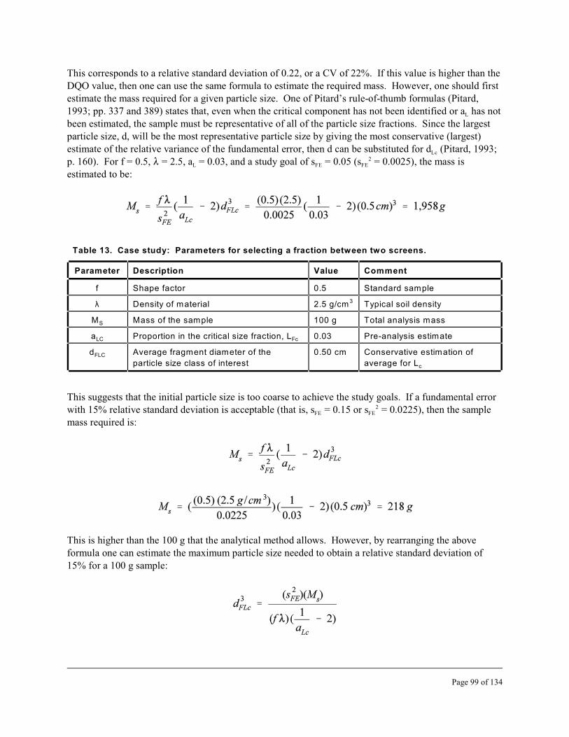
This corresponds to a relative standard deviation of 0.22, or a CV of 22%. If this value is higher than the DQO value, then one can use the same formula to estimate the required mass. However, one should first estimate the mass required for a given particle size. One of Pitard’s rule-of-thumb formulas (Pitard, 1993; pp. 337 and 389) states that, even when the critical component has not been identified or aL has not been estimated, the sample must be representative of all of the particle size fractions. Since the largest particle size, d, will be the most representative particle size by giving the most conservative (largest) estimate of the relative variance of the fundamental error, then d can be substituted for dLc (Pitard, 1993; p. 160). For f = 0.5, 8 = 2.5, a = 0.03, and a study goal of s = 0.05 (s 2 = 0.0025), the mass is L FE FE

estimated to be:

Table 13. Case study: Parameters for selecting a fraction between two screens.

Parameter Description Value Comment

f Shape factor 0.5 Standard sample

8 Density of material 2.5 g/cm 3 Typical soil density

MS Mass of the sample 100 g Total analysis mass

LCa FcProportion in the critical size fraction, L 0.03 Pre-analysis estimate

dFLC Average fragment diameter of the

particle size class of interest

0.50 cm Conservative estimation of

average for L c

This suggests that the initial particle size is too coarse to achieve the study goals. If a fundamental error with 15% relative standard deviation is acceptable (that is, s = 0.15 or sFE

2 = 0.0225), then the sample FE

mass required is:

This is higher than the 100 g that the analytical method allows. However, by rearranging the above formula one can estimate the maximum particle size needed to obtain a relative standard deviation of 15% for a 100 g sample:

Page 99 of 134

This corresponds to a diameter This value is just a little lower than the originally assumed conservative maximum diameter of 0.5 cm. The conclusion would be to process the samples as they arrived rather than go through an extra step for particle size reduction.

8.7 Case Study: Subsampling Designs

(This case study is adapted from: ASTM D 5956, Standard Guide for Sampling Strategies for Heterogeneous Wastes, Second Edition, 1997.) A laboratory received a 1 kg sample of potentially hazardous waste in which one-gram nuggets of cadmium are randomly distributed. The average level of cadmium is to be determined based on the analysis of 10 subsamples (the required analytical mass depends on the design given below). The gangue (matrix) is free of cadmium and has a much smaller particle size than the cadmium. The sample is 33% cadmium by weight and the gangue is similar to fine sand (< 0.25 mm particle diameter) with a density about a third of that for Cd. Cadmium has a density of

38.65 g/cm , and one can estimate the volume (V ), radius (r), and diameter (d) of a sphere of 1 g of Cd Cd

as:

Since the Cd weight fraction of the sample is 33%:

Since the density of Cd is about 3 times that of the gangue, then the volume of one gram of sample is

and the density of the sample is:

Page 100 of 134

The volume fraction of Cd is, therefore:

8.7.1 Subsampling Design A

The subsample mass required for analysis: 0.1 g.

Subsampling method: Select the subsample using a small spatula.

Discussion: None of the Cd nuggets are selected since their mass (one-gram nuggets) is much larger than required by the analytical method, and the Cd nuggets are too big for the size of the spatula. They literally roll off before the spatula leaves the container. Sample analysis results are all less than 1% w/w Cd. The results are not incompatible with assuming a normal distribution, and one falsely concludes the population is uniformly low in Cd.

Conclusion: No significant Cd present; all of the subsamples < 1% w/w Cd with CV < 1%.

Truth: Cd is 33% w/w.

8.7.2 Subsampling Design B

The subsample mass required for analysis: 1.0 g.

Subsampling method:Select the subsample with a much larger spatula with at least an inner diameter of 3 times the size of the Cd nuggets (3d = 1.812 cm); thus, a spatula (parallel side and a square bottom) with an inner diameter of 2 cm should suffice.

Discussion: Some of the subsamples will consist primarily of Cd nuggets, but most will have cadmium levels like those found in Design A. The probability of randomly selecting a Cd nugget (if there is no GE; that is, the sample is perfectly mixed, which is highly unlikely) will be proportional to the volume fraction that is Cd. The probability (p = 0.141) is that 14.1% v/v of the subsamples would be expected to be a Cd nugget. Based on a binomial approximation for the probabilities associated with selecting Cd as the volume fraction, the expected number of the 10 one-gram analytical subsamples being a one-gram Cd nugget is

½0 = np = (10)(0.141) = 1.41, with a standard deviation of s = (npq)½ = [(10)(0.141)(0.859)] = 1.10, where q = 1 - p. This gives a CV of (100%)(1.10/1.41) = 78%. That is, on average, 1.41 of the 10 analytical subsamples would contain a one-gram Cd nugget. In practice, one cannot get a fractional nugget; therefore, the most likely result will be that for the 10 one-gram subsamples taken for analysis, 1 or 2 samples will be a one-gram nugget of Cd (10% v/v or 20% v/v). This discussion will assume that only 1 of the 10 analytical subsamples will be a Cd nugget, resulting in an average Cd level of 0.1 v/v (10% v/v).

Page 101 of 134

Given that most of the subsamples show no Cd (9 of the 10 subsamples taken), the one high Cd value may be mistakenly declared to be an outlier. Suppose that 4 additional analytical subsamples were run to verify the low Cd levels. The probability that none of the 4 subsamples contain a Cd nugget is

4(100%)(0.859) , or 54%. Hence, there is a better than even chance that none of the additional 4 subsamples will show high levels of Cd, helping to confirm the outlier designation. For a discussion on outliers, please refer to Barnett and Lewis (1995) or to Singh and Nocerino (1995). Software has been developed for the methods discussed in the latter reference by Singh and Nocerino; the software is called Scout (Scout, 1999).

Conclusion: The average Cd level is 10% v/v (23% w/w) with a CV = 78% with no outliers claimed; or, the average Cd level is 0% v/v with a CV = 78%, but an occasional hot spot may exist.

Truth: Cd is 14% v/v (33% w/w).

8.7.3 Subsampling Design C

The sample mass required for analysis: 31.25 g.

Subsampling method: Use a sectorial splitter in a two-step process.

Step 1: Divide the 1 kg sample into 8 fractions of 125 g.

Step 2: Divide each 125 g fraction into 4 fractions of 31.25 g.

Discussion:A 1 kg sample with 33% w/w Cd in the form of 1 g nuggets has 333 nuggets. If the sample is equitably partitioned into 32 subsample splits, then the number of nuggets per subsample split should average approximately 10. If an average of 10 nuggets per subsample is expected, then the results should follow a normal probability distribution. The average result from the analysis of 10 subsamples is found to be 32% w/w Cd with a CV of 3%.

Conclusion: The average Cd level is 32% w/w Cd with a CV of 3%.

Truth: Cd is 33% w/w.

While the correct answer is obtained with a large sample mass, one may not be able to obtain it if the analysis is constrained to use only small mass sizes. To get the same or better results when using a small sample mass, the particle distribution of the analyte needs to be altered so that subsampling behaves like Design C instead of Design A. That means that one needs to have a much larger number of small analyte particles. The goal is that each subsample will, on average, have enough analyte particles (greater than 5) to be modeled as a normal distribution.

Page 102 of 134

8.7.4 Subsampling Design D

The sample mass required for analysis: 0.1 g

Subsampling method: Subsampling requires a two-step procedure.

Step 1: The sample is ground to pass through a 0.25 mm mesh.

Step 2: Small spatula (>3d = 0.75 mm is easily achieved) is used, taking many random increments, to obtain each of the 10 subsamples for analysis.

Discussion: For this design the sample must be ground to reduce the maximum particle size from 3.0 mm down to 0.25 mm. For the Cd particles, this is a size reduction of about a factor of 10 in the linear dimension. The mass reduction for Cd particles follows the change in volume and decreases by approximately a factor of 1000 (down to 0.001 g per particle), and, therefore, the number of analyte particles will increase by about 1000-fold. The number of Cd particles per 0.1 g sample can be estimated by noting that 33% of 0.1 g = 0.033 g. If this is the average amount of Cd in the sample, then 33 particles per subsample would be expected and the uncertainty should be well approximated by a normal distribution function, with a CV less than 1%.

Conclusion: Based on a 0.1 g sample, the average level of Cd is 33% w/w with CV < 1%.

Truth: Cd is 33% w/w.

8.8 Case Study: Subsampling Designs Summary

This case study is somewhat simplified in that all of the analyte is in the form of pure particles and no analyte exists in the remaining gangue (matrix). However, it demonstrates that a variety of results may be reported for the average analyte level (see Table 14), and each conclusion appears justified by the supporting data. The difference between correct and incorrect conclusions is due to the analyst’s assumptions about how the analyte is distributed throughout the sample. As noted by Pitard (1993), obtaining the correct answer requires the analyst to either increase the sample mass (Design C) or to decrease the particle size (Design D). Given the added constraint of a small subsample for the analysis, the only design that will give the correct answer is Design D.

All of the procedures would have given the correct answer if Cd was fairly homogeneously distributed across all of the particle types. Overcoming the variability from various heterogeneous factors requires more knowledge about the analyte distribution and the sampling process than initially exists. Determining what information is required is the key to the development of a correct sample mass reduction procedure.

Page 103 of 134

Table 14. A summary of the results from the case study designs.

Case Study Design

Analytical

Sample

Mass, Ms (g)

Cd

(w/w %)

Cd CV

(%RSD) Accuracy

A. Small sample mass 0.1 < 1 < 1 Low

B1. No outlier 1.0 23 78 Moderate

B2. Outlier claimed 1.0 < 1 < 1 Low

C. Larger sample mass 31.25 32 3 High

D. Smaller particle size 0.1 33 < 1 High

Page 104 of 134

Section 9

Reporting Results

9.1 Introduction

Summarizing the results from a study usually requires more than listing simple concentration estimates for individual samples or producing a summary statistic, like the average analyte concentration. Additional information is necessary at several levels if the reported values are to be correctly interpreted. Scientifically sound decisions require the critical assessment of a number of factors describing the study.

As a general guideline for writing the report, give the information that would be produced by developing and following the sampling plan (see the guidance given in the section on “Proposed Strategies”). Give an historical account leading to the study. Include historical and preliminary study information and results. If known, discuss how the laboratory sample was obtained (including the transportation and the chain-of-custody of the sample). Document the sample characterization and assessment observations. List the study objectives (e.g., DQOs) and the rational for their development. Present the sampling plan (include the sampling nomograph if it was used). Describe the analytical method and discuss why it was appropriate for this study. Give the required analytical mass, M . s

Describe any pre-sampling treatments (drying, removing inert debris) and discuss the actions to take (including mass calculation corrections). Report the steps taken to ensure correct sampling practices; give: (1) a description of the subsampling method, (2) a description of the equipment used for correct materialization, (3) the number of increments selected, (4) a description of how those increments were selected, (5) a description of any comminution steps, and (6) a discussion on minimizing the preparation

2error. List the IHL factors used to calculate sFE . Document how the data will be treated (e.g., the propagation of errors), including calculations and graphs. Give estimates of the analyte proportion (a )s

and all of the sampling and analytical errors.

The information needed to evaluate the study is usually presented so that readers with different levels of expertise are not required to read the entire report to find the information that they are interested in. This section describes the type of information, in addition to the analytical and statistical results, that would be of interest to the four previously identified individual types targeted as the intended audience for this guidance document: the analyst, the scientist or statistician, the manager, and the decision maker. Those four individual types may each participate in writing the report or they may just be part of the intended audience. In either case, each has the responsibility to make sure that certain information is presented in the report. Much of that information may be of interest to more than one type of reader; although, most readers will only be interested in a small part of the study. Certainly, most readers will be interested in additional details if unexpected results or procedures were followed.

Page 105 of 134

The report must be written to address the interests and input from each person involved in the measurement process – from designing the sampling plan to taking the samples to making any decisions from the results. Thus, the report must discuss and document all aspects of the study, including: the planning, the execution (sample selection and analysis), the interpretation, and the decision making.

9.2 For the Analyst

The analyst is concerned with accurately documenting the technical execution of the study (subsampling and analysis). Deviation from the sampling plan or the analytical procedure must be noted. The analyst must demonstrate that correct sampling practices were followed and that a suitable analytical method was followed. The analyst should document the data manipulation steps used to process and generate the final analytical results of the study. The analyst should also report the following.

I. State the objectives to be achieved. For example, “analyze for the average concentration of arsenic.” If uncertainty limits were identified for the study, then those should be provided, too.

II. Describe the sample, including: size; mass; physical characteristics, such as particle size range;color; contaminants, such as bottle caps or glass shards, etc.

III. Reference or describe the subsampling process. This includes the protocol for selecting the analytical subsample from the laboratory sample and any sample processing activity.

IV. Describe the subsample, including: The mass of the subsample used in the physical analysis; the maximum particle size in the subsample; any unusual physical characteristics; any differences from the description of the sample; if replicate analyses were used, then report the results (from replicate extractions, replicates of a single extraction, or other type of replicates).

V. Summarize the analytical method. The analytical method should be described, either by reference or, for custom methods or study-dependent sample treatments, with a specific description of the process. The range of the analytical method, historical analytical performance data, known analytical interferences, corrections for analytical bias, and any deviations from the sampling plan or the analytical method must be reported.

Performance criteria for the method should be listed or referenced. However, the study report should contain at least summary results related to performance. If interlaboratory performance data are available, then those figures-of-merit are of interest. However, individual laboratories have unique responses; therefore, the results from the laboratory’s internal calibration, QA, and QC work are of primary interest in demonstrating the level of uncertainty associated with the physical analysis of a subsample.

Those analytical results should provide estimates of the detection limit, quantification limit, relative 2variability (sAE ) as a function of concentration, and bias (m(AE)). The number and type of each

performance statistic depend on the experimental design. The closer the results are to the decision criteria, the more important the performance characterization results will become.

Page 106 of 134

Report the analytical range for the standard curve. This may be different from the range of sample concentrations. An analytical method with a lower concentration range could be used to determine samples with a higher analyte concentration through sample dilution.

VI. Document the procedures affecting the data base. Report the estimated analytical uncertainty and a description of how it was determined.

Give the lower concentration limit for reporting a quantified value. If minimum quantified values are estimated on a sample-by-sample basis, then the report should indicate that.

Describe the laboratory reporting procedure for results below the limit-of-quantification. Often results below the quantification level are reported as sample-specific values. Each sample with low analyte levels may have a different value associated with it in the data base, giving the superficial appearance that a quantified result is present. If an estimated value is provided, it should be clearly marked as such. The algorithm for estimating any non-quantified value should be provided or referenced.

If a value of zero is reported, then the report should indicate if this result is due to the round off of significant figures or if zero was substituted for the measured response. Some samples, such as blanks, may occasionally result in negative concentration estimates. While these are perfectly valid as the measured response, they are often rounded up to zero because it is impossible to have a negative concentration. While this is acceptable when interpreting a data set, it is not acceptable when creating one.

Hypothetical Example: AACME Laboratory confidently converts all of their negative responses to zero prior to entering the analytical results into a data base. No negative values are allowed because no sample has a negative concentration. An analysis for the average response from a set of blanks is later calculated, and the result is a value of 5 ppm Cr; and, based on the number of results, one can claim with great confidence that this value is greater than zero. Unfortunately, this result is a biased estimate. For a true (unbiased, zero) blank, half of the responses should be above zero and half of the responses should be below zero. The average should be indistinguishable from zero. Converting all of the negative numbers to zero artificially biases the data.

If all of the original values from the standard curve were reported, then one could compare the level of Cr from the field samples to those of the blank samples. When negative values are converted to zero, then the comparison is only acceptable if the estimated bias in the standards is small compared to the difference between the samples and the blank. Unfortunately, this is just the situation when accurate statistical models are not needed. When the differences are large, there is little reason to check for statistical relevance. The random low variation near zero is statistically just as important as any random high estimate in the samples with concentrations above the detection level.

VII. Summarize the QA and QC results related to the sample integrity to verify performance. Report the results with regard to any loss or gain from contamination or sample carryover during analysis. Previous performance for the analysis at another laboratory or summarized from an interlaboratory study only suggests that the method will perform as designed. A review of the method performance

Page 107 of 134

as provided by the QA and QC results will provide the only appropriate accuracy and bias estimates for the data set.

9.3 For the Scientists and Statisticians

The scientists and statisticians are concerned with interpreting, evaluating, validating, and summarizing the data generated and reported by the analyst. A list (if practical) and a summary of the data should be presented. How the data were processed should be documented. The report should include an assessment of the effect that sampling and analysis had on the study. The importance of sampling should be assessed in the context of all the other factors that might affect the conclusions as

2 2 2 2 2 2 2part of a standard sensitivity analysis. Estimates of mTE , sTE , rTE , mAE , sAE , m , and s should be OE OE

given. The propagation of errors (e.g., for each subsampling step) must be addressed.

I. Give a summary of all of the sample and data manipulation actions that occurred when the samples were taken, and during the sample processing and analysis stages. For instance, particle size information for particles containing the analyte of interest and for non-analyte containing particles should be reported.

II. Describe the sample history and origin, if known, including any division of the original lot into multiple lots, strata, or batches, such as considering a warehouse or packaging building as one lot, an exterior storage area as a second lot, and an adjacent chemical manufacturing facility as a third lot.

III. Report the results from any preliminary characterization measurements that were used to justify a particular analysis protocol. Give descriptions of the samples, subsamples, analytical method, subsampling method, and the limit-of-quantitation.

IV. Give the performance characteristics of the method. Report the limit-of-quantification (or list representative examples if the limit-of-quantification is determined on a sample-by-sample fashion).

V. Report the percentage of non-quantitative results. For example, report the fraction of results that were below the contract or the method quantitative analysis limits. If more than one analyte is measured, then that limit should be reported on a per analyte basis.

VI. Describe all of the protocols followed in the preparation of the data base. This would include an explanation describing the values inserted into a data base when non-quantitative values are present. A similar explanation is needed if alternate values are substituted for those data base entries when calculating summary statistics. For example, the reader should be informed if the data base contains one-half of the estimated detection limit whenever the concentration was found to be below the quantitation limit. Data bases often contain sample-specific estimates of the detection or quantitation limits that, for all practical appearances, look as if they are quantitative estimates. In reality those non-quantitative artifacts of the data base recording protocol are often an arbitrary guess of the analyte level and may be difficult to recognize.

Page 108 of 134

If the results from below the limit-of-quantitation are included in the summary statistics, then a description of what values were used for those results should be included. For example, report if the concentrations were set to zero, to the limit-of-quantitation, to one-half of the limit-of-quantitation, to a random number between zero and the quantitative limit, or to some other value.

Include equations and example calculations. Explain why, and describe (may be referenced), any uncommon statistical methods that are used (e.g., robust outlier detection methods).

9.4 For the Managers

The manager is concerned with documenting if the study was performed within the design and planning specifications, and if the study objectives were met. Anomalies and deviations must be documented, discussed, and explained. The results provided by the analyst, and the scientist or statistician, should be summarized and verified. The manager must be sure that the mass data have been corrected for any pre-sampling actions, such as drying or removing inert objects, as identified in the sampling plan. The manager should be able to validate if correct sampling practices were followed (e.g.,

2 2does sTE . sFE ?) and that a representative sample was obtained within the limits set by study objectives 2 2(r # r0TE ). The manager must verify that the study interpretations are defensible. Besides reporting if TE

the results meet the technical requirements, the manager may also discuss cost and benefit issues. It is the manager’s responsibility to make sure that the information that the decision maker sees is informative, accurate, and reliable. Managers should see or report the same information as the decision makers, but with the added level of detail summarized below.

I. Report whether or not the sample description is compatible with the sample treatment. If the samples have particle sizes that suggest that particle size reduction is needed but the sample treatment did not include that step, then the sampling protocol may be incorrect.

II. Describe and discuss the statistical results. If the distribution of the data is highly skewed and the fraction of samples with below detection values is large, then there should be a discussion of the sample mass and subsampling practices. This becomes more important as the skewness increases or as the fraction of the samples with below the quantitative levels of the analyte increases. In either case, the estimate of the mean analyte concentration(s) becomes less certain and more dependent on the sample characteristics.

III. The concentration (or concentration ranges) dividing the non-quantitative from the quantitative results should be identified. Flags should identify any substituted values. There should also be an assessment if the assumptions made to fill in values for an analysis are influential with respect to the decisions being made. If the results are influenced by the fill-in procedure, then they are more than likely to be unstable and probably will not justify a decision.

IV. Review the fraction of the samples with low, non-quantitative results. If that fraction is large, then the treatment of below quantitative data may play an important role in determining the true analyte level.

Page 109 of 134

V. Discuss any outliers identified in the data base. If any outliers were not included in any of the calculations or in the data base, then give a justification for their removal. For a discussion on outliers, please refer to Barnett and Lewis (1995) or to Singh and Nocerino (1995). Software has been developed for the methods discussed in the latter reference by Singh and Nocerino; the software is called Scout (Scout, 1999).

VI. Give any estimates of measurement reproducibility and sources of variation. If possible, those estimates should be partitioned into sources of variation.

9.5 For the Decision Makers

The decision maker is concerned with the implications of the study for what to do next. The decision maker needs to be sure that the information reported or verified by the manager is informative, accurate, and reliable so that correct (informative, accurate, and reliable) decisions can be made. Supporting evidence should be summarized showing that correct and representative sampling took place, and that it is reasonable to believe that the average proportion of the analyte in the analytical subsample is the same, within the user-specified study objectives, as the average proportion of the analyte in the laboratory sample; that is, a . a . At a minimum, the decision maker should note whether or not sampling concerns s L

are addressed, but should extend to evaluating whether or not the study activities met the cost and benefit goals, resulted in acceptable risks, and met legal and policy requirements.

I. Give a clear statement of the issues and the factors that were considered in setting the study objectives. Determine if the study results are accompanied by some measure of sensitivity that identifies if there is a clearly supported action suggested by the data or whether the data did not meet the pre-study requirements. Give any evidence to suggest that the response is associated with enough variability to justify delaying action.

II. Document the number and location of the samples. If the samples were taken during several sampling events, then an indication of the time sequence should be present. If different laboratories or analysis times were used to generate data, then the procedure and results for ensuring the comparability of different data sets should be provided as well as key summary statistics.

III. Include the key features of the data, including the minimum concentration for quantitation, the fraction of samples (by analyte) with results below this level, and the concentration of concern. A description of how a typical sample was taken, the sample processing step(s), and the analytical method used should be given.

Page 110 of 134

Section 10

Summary and Conclusions

The characteristics of samples collected from a lot are used to make estimates of the characteristics of that lot. Thus, samples are used to infer properties about the lot in order to make correct decisions concerning that lot. Therefore, for sampling to be meaningful, it is imperative that a sample is as representative as possible of the lot, and more generally, each subsample must be as representative as possible of the parent sample from which it is derived. Subsampling errors propagate down the chain from the largest primary sample to the smallest laboratory analytical subsample. If a collection of samples does not represent the population from which they are drawn, then the statistical analyses of the generated data may lead to misinformed conclusions and perhaps costly decisions.

Sampling can be the major source of error in the measurement process and it can be an especially overwhelming source of error for heterogenous particulate materials, such as soils. Since classical statistical sampling theory is not adequate for such samples, the Pierre Gy statistical sampling theory was introduced in this document as a viable alternative that takes into account the nature of particulate materials. Although this theory, developed in the mid-1950s, has proven itself in practice in the mining industry, very little has been published with substantiating experimental evidence for this theory. An ongoing research program has been established to experimentally verify the application of the Gy theory to environmental samples, which served as a supporting basis for the material presented in this guidance. Research results from studies by the U.S. EPA have confirmed that the application of the Gy sampling theory to environmental heterogeneous particulate materials is the appropriate state-of-the-science approach for obtaining representative laboratory subsamples.

This document provided general guidelines for obtaining representative subsamples for the laboratory analysis of particulate materials using “correct” sampling practices and “correct” sampling devices. Besides providing background and theory, this document gave guidance on: sampling and comminution tools, sample characterization and assessment, developing a sampling plan using a general sampling strategy, and reporting recommendations. Considerations were given to: the constitution and the degree of heterogeneity of the material being sampled, the methods used for sample collection (including what proper tools to use), what it is that the sample is supposed to represent, the mass (sample support) of the sample needed to be representative, and the bounds of what “representative” actually mean. A glossary and a comprehensive bibliography have been provided and should be consulted for more details.

The basic strategic theme developed in this document concluded that if “correct” sampling practices are followed and “correct” sampling devices are used, then all of the sampling errors should become negligible, except for the minimum sampling error that is fundamental to the physical and chemical composition of the material being sampled. That is, the mean of the total sampling error becomes

Page 111 of 134

negligible (no sampling bias) and the relative variance of the total sampling error is reduced to the 2 2relative variance of the fundamental error (s = sFE ). Since this minimum fundamental sampling error TE

can be estimated before any sampling takes place, sFE2 can be used to develop a sampling plan.

It was shown that correct sampling (or selection) can be associated with three practices: 1) correctly taking many increments (greater than about 30 are recommended) to make up the subsample to minimize the grouping and segregation error (GE), 2) using correctly designed sampling tools to minimize the materialization error (ME), and 3) using common sense and vigilance to minimize the preparation error (PE).

The bounds of what are acceptable for a sample to be “representative” of the lot are set by the study objectives (e.g., the data quality objectives or DQOs). The degree of representativeness, r 2, has been TE

2 2 2defined in this document by r = mTE2 + sTE , where TE is the total sampling error, r is the mean TE TE 2 2square of the total sampling error, m is the square of the mean of the total sampling error, and s isTE TE

2 2 2the relative variance of the total sampling error. A sample is representative when r # roTE , where r TE oTE

is a specified and quantitative measure of a representative sample (the smaller this number, the more representative is the sample); that is, it is a level of representativeness regarded as acceptable (usually set by the study objectives). If correct sampling practices are applied and all of the “controllable” errors are minimized, then a representative sample could be characterized by keeping the relative variance of the

2 2 2fundamental error below a specified level, s # soFE2. Under such conditions, r . sFE

2 # soFE . roTE2.FE TE

This equation served as the basis of our strategy to obtain a representative analytical subsample. This is fortuitous for our planning purposes, and for formulating our study objectives (e.g., DQOs), since s 2 isFE

the only error that can be calculated, based on the physical and chemical properties of the particulate material, a priori; that is, before sampling even takes place!

Page 112 of 134

Recommendations

For those familiar with most of the information given in this guidance, it was suggested that such a user, searching for the guidance to develop a sampling plan to obtain a representative analytical subsample, go to the section on “Proposed Strategies,” which gives a general and somewhat extensive sampling strategy guide.

The guidance presented is general and is not limited to environmental samples, and is applicable to samples analyzed in the field. The information given in this guidance should also prove to be useful in making reference standards as well as taking samples from reference standards. Similarly, the presented guidance should be of value in: Monitoring laboratory performance, creating performance evaluation materials (and how to sample them), certifying laboratories, running collaborative trials, and performing method validations.

Remember that sampling is one of those endeavors that you “get what you pay for,” at least in terms of effort. But, with the right knowledge and a good sampling plan, the effort is not necessarily that much. It pays to have a basic understanding of the theory. Become familiar with what causes the different sampling errors and how to minimize them through correct sampling practices. Be able to specify what constitutes a representative subsample. Know what your sampling tools are capable of doing and if they can correctly select an increment. Always do a sample characterization (at least a visual inspection) first. At a minimum, always have study objectives and a sampling plan for each particular case. If possible, take a team approach when developing the study objectives and the sampling plan. Historical data or previous studies should be reviewed. And be sure to record the entire process!

This guidance focused on the issues and actions related to samples composed of particulate materials. It is not intended for samples selected for analysis of volatile or reactive constituents, and it does not extend to sampling biological materials, aqueous samples, or viscous materials, such as grease or oil trapped in a particulate matrix. Such cases warrant more research and guidance. Correct sampling practices to obtain representative field samples should also be the subject of ongoing research and a future guidance document.

Page 113 of 134

Page 114 of 134

References

Allen, T. 1997. Particle Size Measurement, Vol. 1, Fifth Edition. Chapman & Hall, London.

Allen, T., Khan, A.A. 1970. “Critical Evaluation of Powder Sampling Procedures,” Chemical Engineer (London), Vol. 238, pp. CE108-CE112.

ASTM. 1997. ASTM Standards on Environmental Sampling. Second Edition. ASTM, West Conshohocken, PA.

Barnett, V., Lewis, T. 1994. Outliers in Statistical Data. Wiley, NY.

Barth, D.S., Mason, B.J., Starks, T.H., Brown, K.W. 1989. Soil Sampling Quality Assurance User’s Guide, Second Edition, EPA/600/8-89/046, U.S. Environmental Protection Agency, Las Vegas, NV.

Dixon, W.J., Massey, F.J., Jr. 1969. Introduction to Statistical Analysis, Third Edition, McGraw-Hill, New York.

Francois-Bongarcon, D., Gy, P. 1999. The most common error in applying “Gy’s Formula” in the theory of mineral sampling. Australian Journal of Mining.

Gerlach, R.W., Dobb, D.E., Raab, G.A., Nocerino, J.N. 2002. Gy Sampling Theory in Environmental

Studies I: Assessing Soil Splitting Protocols. Journal of Chemometrics, 16(7), 871-878.

Gy, P.M. 1982. Sampling of Particulates – Theory and Practice, Second Edition, Elsevier, Amsterdam.

Gy, P.M. 1998. Sampling for Analytical Purposes. Wiley, Chichester, UK.

Ingamells, C.O. 1976. Derivation of the sampling constant equation. Talanta, 23, 263-264.

Ingamells, C.O., Pitard, F.F. 1986. Applied Geochemical Analysis. Wiley, NY.

Ingamells, C.O., Switzer, P. 1973. A proposed sampling constant for use in geochemical analysis.

Talanta, 20, 547-568.

Kern, A.M., Evans, J.D., Hayes, S.L., Partymiller, K.G., Swanson, G.R. 1997. Representative sampling and analysis of heterogeneous soils. Environmental Testing & Analysis, pp. 20-22, 27.

Page 115 of 134

Mason, B.J. 1992. Preparation of Soil Sampling Protocols: Sampling Techniques and Strategies. EPA/600/R-92/128, Environmental Monitoring Systems Laboratory, U.S. Environmental Protection Agency, Las Vegas, NV.

Mishalanie, E., Ramsey, C. 1999. Obtaining Trustworthy Environmental Data: Sampling and Analysis

Issues. Natural Resources & Environment, Vol. 13(4), 522-527.

Mullins, C.E., Hutchinson, B.J. 1982. The variability introduced by various subsampling techniques.

Journal of Soil Science, 33, 547-561.

Myers, J.C. 1996. Geostatistical Error Management: Quantifying Uncertainty for Environmental Sampling and Mapping. Van Nostrand Reinhold, NY.

Pitard, F.R. 1993. Pierre Gy’s Sampling Theory and Sampling Practice: Heterogeneity, Sampling Correctness, and Statistical Process Control, Second Edition. CRC Press, Boca Raton, FL.

Ramsey, C.A., Ketterer, M.E., Lowery, J.H. 1989. Application of Gy’s Sampling Theory to the Sampling of Solid Waste Materials. In: Proceedings of the EPA Fifth Annual Waste Testing and Quality Assurance Symposium, pp. II-494.

Singh, A., Nocerino, J.M. 1995. “Robust Procedures for the Identification of Multiple Outliers.” A chapter in Chemometrics in Environmental Chemistry, J. Einay, ed., a volume in The Handbook of Environmental Chemistry, O. Hutzinger, ed. (Heidelberg, Springer-Verlag).

“Scout: A Data Analysis Program” (revised March 1999), Technology Support Bulletin, U.S. EPA, EMSL-LV, Las Vegas, NV 89193-3478.

Smith, P.L. 2001. A Primer for Sampling Solids, Liquids, and Gases Based on the Seven Sampling Errors of Pierre Gy. Society for Industrial and Applied Mathematics, Philadelphia, PA.

Starr, J.L., Parkin, T.B., Meisinger, J.J. 1995. Influence of Sample Size on Chemical and Physical Soil

Measurements. Soil Science Society of America Journal, 59, 713-719.

U.S. EPA. 1986. Test methods for evaluating solid waste, physical/chemical methods. Vol. 2, Part III, Sampling, Third edition. EPA/SW-846, Office of Solid Waste and Emergency Response, U.S. Environmental Protection Agency, Washington, DC.

U.S. EPA. 1994. Guidance for the Data Quality Objectives Process (EPA QA/G-4). EPA/600/R-96/056, Office of Research and Development, U.S. Environmental Protection Agency, Washington, DC.

U.S. EPA. 1996a. The Data Quality Evaluation Statistical Toolbox (DataQUEST) Software (EPA QA/G-9D). U.S. Environmental Protection Agency, Office of Research and Development, Washington, DC.

U.S. EPA. 1996b. Soil Screening Guidance: User’s Guide. EPA/540/R-96/0180. U.S. Environmental Protection Agency, Office of Solid Waste and Emergency Response, Washington, DC.

Page 116 of 134

U.S. EPA. 1996c. Guidance for Data Quality Assessment: Practical Methods for Data Analysis, (EPA QA/G-9). EPA/600/R-96/084, U.S. Environmental Protection Agency, Office of Research and Development, Washington, DC.

U.S. EPA. 1997. Data Quality Assessment Statistical Toolbox (DataQUEST), (EPA QA/G-9D). EPA/600/R-96/085, Office of Research and Development, U.S. Environmental Protection Agency, Washington, DC.

U.S. EPA. 1998. Guidance for Quality Assurance Project Plans, (EPA QA/G-5). EPA/00/R-98/018), U.S. Environmental Protection Agency, Washington, DC.

U.S. EPA. 2000a. Guidance for the Data Quality Objectives Process, (EPA QA/G-4), EPA/600/R-96/055, Office of Environmental Information, U.S. Environmental Protection Agency, Washington, DC.

U.S. EPA. 2000b. Guidance for Choosing a Sampling Design for Environmental Data Collection, EPA QA/G-5S, Peer Review Draft, Office of Environmental Information, U.S. Environmental Protection Agency, Washington, DC, 156 p.

U.S. EPA. 2000c. Guidance for Technical Assessments, (EPA QA/G-7). EPA/600/R-99/080. U.S. Environmental Protection Agency, Washington, DC.

U.S. EPA. 2000d. Data Quality Objectives Process for Hazardous Waste Site Investigations, (EPA QA/G-4HW). EPA/600/R-00/007, U.S. Environmental Protection Agency, Office of Environmental Information, Washington, DC.

van Ee, J., Blume, L.J., Starks, T.H. 1990. A rationale for the assessment of errors in the sampling of soils. EPA/600/4-90/013, Environmental Monitoring Systems Laboratory, U.S. Environmental Protection Agency, Las Vegas, NV, 63 p.

Visman, J. 1969. A general theory of sampling. Materials Research and Standards, 9, 8-13.

Page 117 of 134

Page 118 of 134

Bibliography

1. Allen, T. 1977. Particle Size Measurement, Vol. 1, Fifth Edition, Chapman & Hall, London.

2. Allen, T., Khan, A.A. 1970. “Critical Evaluation of Powder Sampling Procedures,” Chemical

Engineer (London), 238, pp. CE108-CE112.

3. ASTM. 1997. ASTM Standards on Environmental Sampling, Second Edition. ASTM, WestConshohocken, Pennsylvania.

4. Barth, D.S., Mason, B.J., Starks, T.H., Brown, K.W. 1989. Soil Sampling Quality AssuranceUser’s Guide, Second Edition. EPA/600/8-89/046, U.S. Environmental Protection Agency, LasVegas, Nevada.

5. Benedetti-Pichler, A.A. 1956. Theory and Principles of Sampling for Chemical Analysis. In:Berl, W.G. (Ed.), Physical Methods in Chemical Analysis, Vol. 3, pp 183-217, Academic Press,New York.

6. Cochran, W.G. 1977. Sampling Techniques, Third Edition. Wiley, New York.

7. Cressie, N. 1993. Statistics for Spatial Data, Revised Edition. Wiley, New York.

8. Davies, R. 1991. Sampling: Solids. In: Kirk-Othmer Encyclopedia of Chemical Technology,Fourth Edition. Vol. 21, 644-650.

9. Davis, J. 1986. Statistics and Data Analysis in Geology, Second Edition. Wiley, New York.

10. Dixon, W.J., Massey, F.J., Jr. 1969. Introduction to Statistical Analysis, Third Edition, McGraw-Hill, New York.

11. Francois-Bongarcon, D. 1993. Geostatistical tools for the determination of fundamental sampling variances and minimum sample masses. In: Geostatistics Troia ‘92; Quantitative Geology and Geostatistics, A. Soares (Ed.), Kluwer Academic Pub., Vol. 2, 989-1000.

12. Francois-Bongarcon, D. 1998a. Extensions to the demonstration of Gy’s formula. Exploration

and Mining Geology, 7(1-2), 149-154.

13. Francois-Bongarcon, D. 1998b. Error variance information from paired data: Applications to

sampling theory. Exploration and Mining Geology, 7(1-2), 161-165.

Page 119 of 134

14. Francois-Bongarcon, D. 1998c. Gy’s formula: Conclusion of a new phase of research. Australian Association of Geoscientists, Vol. 22. <www.gonow.to/goodsampling>

15. Francois-Bongarcon, D., Gy, P. 1999. The most common error in applying “Gy’s Formula” in the theory of mineral sampling. Australian Journal of Mining.

16. Frempong, P.K. 1999. The development of a robust sampling strategy and protocol in underground

gold mines. The Australasian Institute of Mining and Metallurgy Proceedings, 304(2), 15-22.

17. Fricke, G.H., Mischler, P.G., Staffieri, F.P., Housmyer, C.L. 1987. Sample weight as a function of

particle sizes in two-component mixtures. Analytical Chemistry, 59, 1213-1217.

18. Garner, F.C., Stepanian, M.A., Williams, L.R. 1988. Composite sampling for environmental monitoring. Chapter 25 In: Keith, L.H. (Ed.), Principles of Environmental Sampling, American Chemical Society, Washington, DC.

19. Gerlach, R.W., Dobb, D.E., Raab, G.A., Nocerino, J.N. 2002. Gy Sampling Theory in

Environmental Studies I: Assessing Soil Splitting Protocols. Journal of Chemometrics, 16(7), 871­878.

20. Gilbert, R.O. 1987. Statistical Methods for Environmental Pollution Monitoring. Van Nostrand Reinhold, New York.

21. Gy, P.M. 1982. Sampling of Particulates – Theory and Practice, Second Edition. Elsevier, Amsterdam.

22. Gy, P.M. 1992. Sampling of Heterogeneous and Dynamic Material Systems. In: Theories of Heterogeneity, Sampling and Homogenizing. Elsevier, Amsterdam.

23. Gy, P.M. 1998. Sampling for Analytical Purposes. Wiley, Chichester, UK.

24. Hatton, T.A. 1977. Representative sampling of particles with a spinning riffler: A stochastic

model. Powder Technology, 19, 227-233.

25. Horwitz, W. 1988. Sampling and preparation of sample for chemical examination. Journal of the

Association of Official Analytical Chemists, 71(2), 241-245.

26. Ingamells, C.O. 1974. Control of geochemical error through sampling and subsampling designs.

Geochimica et Cosmochimica Acta, 38, 1255-1237.

27. Ingamells, C.O. 1976. Derivation of the sampling constant equation. Talanta, 23, 263-264.

28. Ingamells, C.O. 1978. A further note on the sampling constant equation. Talanta, 25, 731-732.

29. Ingamells, C.O. 1981. Evaluation of skewed exploration data – The nugget effect. Geochimica et

Cosmochimica Acta, 45, 1209-1216.

Page 120 of 134

30. Ingamells, C.O., Pitard, F.F. 1986. Applied Geochemical Analysis. Wiley, New York.

31. Ingamells, C.O., Switzer, P. 1973. A proposed sampling constant for use in geochemical analysis,

Talanta, 20, 547-568.

32. Jenkins, J.F., Grant, C.L., Brar, G.S., Thorne, P.G., Schumacher, P.W., Rannaey, T.A. 1997. Sampling error associated with collection and analysis of soil samples at TNT-contaminated sites.

Field Analytical Chemistry and Technology, 1(3), 151-163.

33. Journel, A.G., Huijbregts, C.J. 1978. Mining Geostatistics. Academic Press, London.

34. Keith, L.H. 1988. Principles of Environmental Sampling. American Chemical Society, Washington, DC.

35. Kern, A.M., Evans, J.D., Hayes, S.L., Partymiller, K.G., Swanson, G.R. 1997. Representative sampling and analysis of heterogeneous soils. Environmental Testing & Analysis, pp. 20-22, 27.

36. Lame, F.P.L., Deflze, P.R. 1993. Sampling of contaminated soil: Sampling error in relation to

sample size and segregation. Environmental Science & Technology, 27(10), 2035-2044.

37. Lopez-Avila, V. (Ed.) 1998. Current Protocols in Field Analytical Chemistry. Wiley, New York.

38. Mason, B.J. 1992. Preparation of Soil Sampling Protocols: Sampling Techniques and Strategies. EPA/600/R-92/128, Environmental Monitoring Systems Laboratory, U.S. Environmental Protection Agency, Las Vegas, NV.

39. Mishalanie, E., Ramsey, C. 1999. Obtaining Trustworthy Environmental Data: Sampling and

Analysis Issues. Natural Resources & Environment, Vol. 13(4), 522-527.

40. Mullins, C.E., Hutchinson, B.J. 1982. The variability introduced by various subsampling

techniques. Journal of Soil Science, 33, 547-561.

41. Myers, J.C. 1996. Geostatistical Error Management: Quantifying Uncertainty for Environmental Sampling and Mapping. Van Nostrand Reinhold, New York.

42. NAVFAC and U.S.EPA. 1998. Field Sampling and Analysis Technologies Matrix and Reference Guide. EPA/542/B-98/002, Naval Facilities Engineering Command and U.S. Environmental Protection Agency, Cincinnati, Ohio.

43. Pitard, F.F. 1989. Pierre Gy’s Sampling Theory and Sampling Practice, Vol. 1, Heterogeneity and Sampling. CRC Press, Boca Raton, FL.

44. Pitard, F.F. 1989. Pierre Gy’s Sampling Theory and Sampling Practice, Vol. 2, Sampling Correctness and Sampling Practice. CRC Press, Boca Raton, FL.

Page 121 of 134

45. Pitard, F.R. 1993. Pierre Gy’s Sampling Theory and Sampling Practice: Heterogeneity, Sampling Correctness, and Statistical Process Control, Second Edition. CRC Press, Boca Raton, FL.

46. Ramsey, C.A., Ketterer, M.E., Lowery, J.H. 1989. Application of Gy’s Sampling Theory to the Sampling of Solid Waste Materials. In: Proceedings of the EPA Fifth Annual Waste Testing and Quality Assurance Symposium, pp. II-494.

47. Schumacher, B.A., Shines, K.C., Burton, J.V., Papp, M.L. 1990. Comparison of Three Methods

for Soil Homogenization. Soil Science Society of America Journal, 54, 1187-1190.

48. Smith, P.L. 2001. A Primer for Sampling Solids, Liquids, and Gases Based on the Seven Sampling Errors of Pierre Gy. Society for Industrial and Applied Mathematics, Philadelphia, PA.

49. Soil Survey Staff. 1993. Soil Survey Manual. Handbook Number 18, U.S. Department of Agriculture, Washington, DC.

50. Starr, J.L., Parkin, T.B., Meisinger, J.J. 1995. Influence of Sample Size on Chemical and Physical

Soil Measurements. Soil Science Society of America Journal, 59, 713-719.

51. Thompson, S.K. 1992. Sampling. Wiley, New York.

52. USDA Soil Survey Staff. 1993. Soil Survey Manual. Handbook Number 18. U.S. Department of Agriculture, Washington, D.C.

53. U.S. DOE. 1992. DOE Methods for Evaluating Environmental and Waste Management Samples. S.C. Goheen, et al., (Eds.), Pacific Northwest Laboratory, Richland, WA.

54. U.S. EPA. 1986. Test methods for evaluating solid waste, physical/chemical methods. Vol. 2, Part III, Sampling, Third edition. EPA/SW-846, U.S. Environmental Protection Agency, Office of Solid Waste and Emergency Response, Washington, DC.

55. U.S. EPA. 1991. Description and Sampling of Contaminated Soils; A Field Pocket Guide. EPA/625/12-91/002, U.S. Environmental Protection Agency, Cincinnati, OH, 122 p.

56. U.S. EPA. 1993. The Data Quality Objectives Process for Superfund: Interim Final Guidance. EPA/540/R-93/071. U.S. Environmental Protection Agency, Office of Emergency and Remedial Response. Washington, DC.

57. U.S. EPA. 1994. Guidance for the Data Quality Objectives Process (EPA QA/G-4). EPA/600/R-96/056, U.S. Environmental Protection Agency, Washington, DC.

58. U.S. EPA. 1996a. The Data Quality Evaluation Statistical Toolbox (DataQUEST) Software (EPA QA/G-9D). U.S. Environmental Protection Agency, Office of Research and Development, Washington, DC.

Page 122 of 134

59. U.S. EPA. 1996b. Soil Screening Guidance: User’s Guide. EPA/540/R-96/0180. U.S. Environmental Protection Agency, Office of Solid Waste and Emergency Response, Washington, DC.

60. U.S. EPA. 1996c. Guidance for Data Quality Assessment: Practical Methods for Data Analysis, (EPA QA/G-9). EPA/600/R-96/084, U.S. Environmental Protection Agency, Office of Research and Development, Washington, DC.

61. U.S. EPA. 1997. Data Quality Assessment Statistical Toolbox (DataQUEST), (EPA QA/G-9D). EPA/600/R-96/085, U.S. Environmental Protection Agency, Office of Research and Development, Washington, DC.

62. U.S. EPA. 1998. Guidance for Quality Assurance Project Plans, (EPA QA/G-5). EPA/00/R-98/018), U.S. Environmental Protection Agency, Washington, DC.

63. U.S. EPA. 2000a. Guidance for the Data Quality Objectives Process, (EPA QA/G-4), EPA/600/R-96/055, U.S. Environmental Protection Agency, Office of Environmental Information, Washington, DC.

64. U.S. EPA. 2000b. Guidance for Choosing a Sampling Design for Environmental Data Collection, EPA QA/G-5S, Peer Review Draft, Office of Environmental Information, U.S. Environmental Protection Agency, Washington, DC, 156 p.

65. U.S. EPA. 2000c. Guidance for Technical Assessments, (EPA QA/G-7). EPA/600/R-99/080. U.S. Environmental Protection Agency, Washington, DC.

66. U.S. EPA. 2000d. Data Quality Objectives Process for Hazardous Waste Site Investigations, (EPA QA/G-4HW). EPA/600/R-00/007, U.S. Environmental Protection Agency, Office of Environmental Information, Washington, DC.

67. van Ee, J., Blume, L.J., Starks, T.H. 1990. A rationale for the assessment of errors in the sampling of soils. EPA/600/4-90/013, U.S. Environmental Protection Agency, Environmental Monitoring Systems Laboratory, Las Vegas, NV, 63 p.

68. Visman, J. 1969. A general theory of sampling. Materials Research and Standards, 9(11), 8-13.

69. Zhang, R., Warrick, A.W., Myers, D.E. 1990. Variance as a function of sample support size.

Mathematical Geology, 22(1), 107-121.

Page 123 of 134

Page 124 of 134

Glossary of Terms

Words highlighted in bold letters within the glossary definitions can be found elsewhere in the glossary with their own definitions.

accuracy – Unfortunately, this term suffers from an extraordinary number of definitions, which can lead to confusion and outright disdain for the word. However, it is still a viable word with correct usage. Accuracy is a degree, or measurement, of closeness to a target value. Accuracy should not be

confused with precision. A sample is accurate if the absolute value of the bias of the total

sampling error is within a specified acceptable level of accuracy:

analytical error (AE) – This error component arises from imperfections in the analysis (chemical or physical) operation. It includes errors associated with such activities as chemically extracting the

analyte from the sample matrix, instrumentation error, operator errors, moisture analysis, gravimetric errors, and other measurement errors.

bias – The systematic or persistent distortion of a measurement process that causes errors in one direction along a metric away the true value; that is, bias is a function of systematic error (e.g., the average measured mass differs from the true mass by +0.034 g). In the context of sampling, bias

(B ) is the mean of the total sampling error, mTE, or as

where mas is the mean estimate of the proportion of the analyte in the sample and a is the true L

proportion of the analyte in the lot.

coefficient of cubicity (f) – See shape factor.

comminution – Comminution is a crushing or grinding process used to decrease the particle size of a lot or a sample.

composite sample – A sample created by combining several distinct subsamples.

composition factor (c) – See mineralogical factor.

Page 125 of 134

continuous selection error (CE) - This error is generated by the immaterial selection process and is the

sum of three errors, the short-range fluctuation error (CE ), the long-range heterogeneity 1

fluctuation error (CE ), and the periodic heterogeneity fluctuation error (CE ):2 3

CE = CE + CE + CE . 1 2 3

correct sampling practice - Correct sampling gives each item (particle, fragment) an equal and constant

probability of being selected from the lot to be part of the sample. Likewise, any item that is not considered to be part of the lot (that is, should not be represented by the sample) should have a zero

probability of being selected. Note that the bias of the total sampling error should be zero (m 2 = TE

0) when the sampling practices are perfectly correct (that is, when GE = DE = EE = PE = 0). If 2 2 2sampling practices are perfectly correct (that is, s = sDE

2 = sEE = sPE2 = 0), then s = sFE

2 (theGE TE

relative variance of the fundamental error). Thus, correct sampling practices minimize those “controllable” errors through correctly designed sampling devices (to minimize DE, sDE

2, EE, and 2 2sEE ), common sense (to minimize PE and s ), and by correctly taking many random increments (NPE

2$30) combined (to minimize GE and s ) to make up the sample. Correct sampling practices allow a GE

representative sample to be taken.

data quality objectives (DQOs) – Qualitative and quantitative statements derived from the DQO process that clarify study objectives, define the appropriate types of data, and specify tolerable levels of potential decision errors that will be used as the basis for establishing the quality and quantity of the data needed to support decisions.

data quality objective (DQO) process – A systematic planning tool to facilitate the planning of environmental data collection activities (see: U.S. EPA, 1994, 1996a, 1996c, 1997, 2000a, and 2000d). The DQO process allows planners to focus their planning efforts by specifying the intended

use of the data, the decision criteria, and the decision maker’s tolerable decision error rates. Data

quality objects are the qualitative and quantitative outputs from the DQO process.

defensible – The ability to withstand a reasonable challenge related to the veracity, integrity, or quality of the logical, technical, or scientific approach taken in a decision making process.

dimension (of a lot) – If the components of a lot are related by location in space or time, then they are associated with a dimension. The dimension of a lot is the number of major axes having an ordered metric. Dimensions in the characterization of a lot become reduced when one or more dimensions

become negligible when compared to the other dimension(s). Sampling units, such as bags of charcoal or bottles of beer from a production line, represent one dimensional lots, with the time of production giving order to the individual items. A zero-dimensional lot has no order to the sampling units. An elongated pile is a one-dimensional lot since it has one major ordered direction. Surface contamination at an electrical transformer storage site represents a two-dimensional lot. Higher (two-, and especially three-) dimensional lots tend to be much more difficult to sample in producing

laboratory subsamples.

estimate – A measured value that approximates the true value. In this text, the proportion of the analyte

in the sample, a , is an estimate of the true proportion of the analyte in the lot, a . Measurements are s L

always subject to errors and one can never claim that the measured value is exactly correct. This is

Page 126 of 134

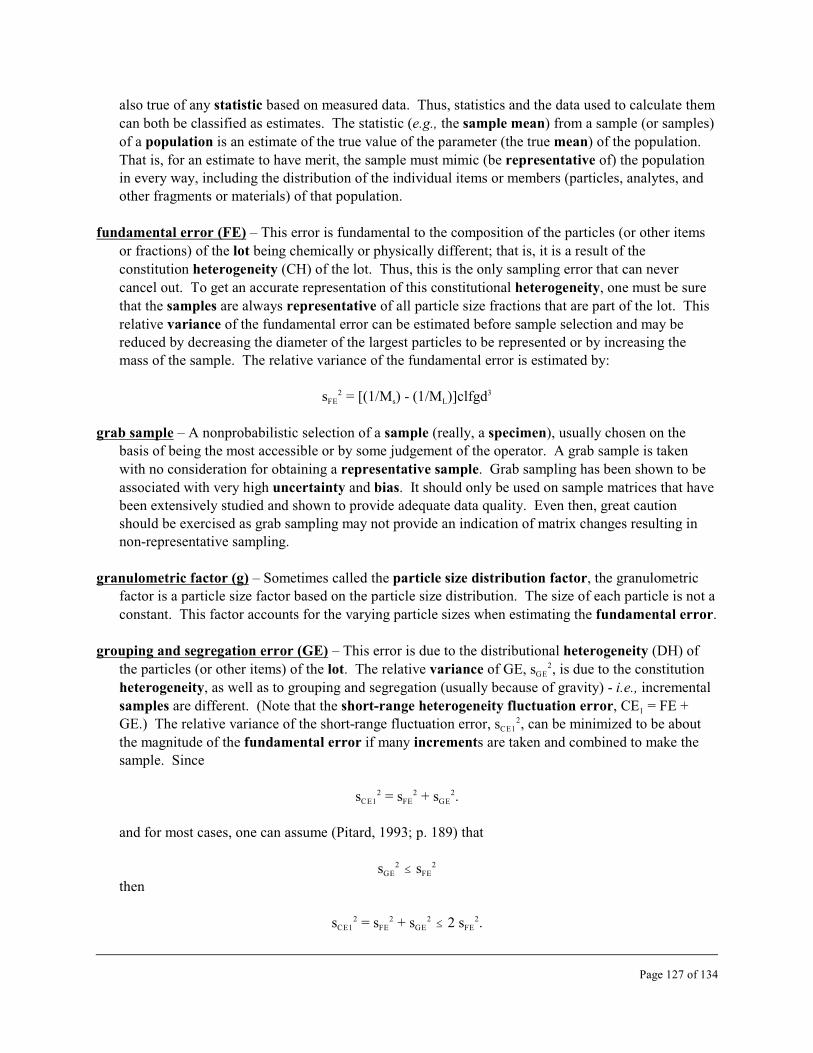
also true of any statistic based on measured data. Thus, statistics and the data used to calculate them

can both be classified as estimates. The statistic (e.g., the sample mean) from a sample (or samples)

of a population is an estimate of the true value of the parameter (the true mean) of the population.

That is, for an estimate to have merit, the sample must mimic (be representative of) the population in every way, including the distribution of the individual items or members (particles, analytes, and other fragments or materials) of that population.

fundamental error (FE) – This error is fundamental to the composition of the particles (or other items

or fractions) of the lot being chemically or physically different; that is, it is a result of the

constitution heterogeneity (CH) of the lot. Thus, this is the only sampling error that can never

cancel out. To get an accurate representation of this constitutional heterogeneity, one must be sure

that the samples are always representative of all particle size fractions that are part of the lot. This

relative variance of the fundamental error can be estimated before sample selection and may be reduced by decreasing the diameter of the largest particles to be represented or by increasing the mass of the sample. The relative variance of the fundamental error is estimated by:

3sFE2 = [(1/M ) - (1/M )]clfgd s L

grab sample – A nonprobabilistic selection of a sample (really, a specimen), usually chosen on the basis of being the most accessible or by some judgement of the operator. A grab sample is taken

with no consideration for obtaining a representative sample. Grab sampling has been shown to be

associated with very high uncertainty and bias. It should only be used on sample matrices that have been extensively studied and shown to provide adequate data quality. Even then, great caution should be exercised as grab sampling may not provide an indication of matrix changes resulting in non-representative sampling.

granulometric factor (g) – Sometimes called the particle size distribution factor, the granulometric factor is a particle size factor based on the particle size distribution. The size of each particle is not a

constant. This factor accounts for the varying particle sizes when estimating the fundamental error.

grouping and segregation error (GE) – This error is due to the distributional heterogeneity (DH) of

the particles (or other items) of the lot. The relative variance of GE, s 2, is due to the constitution GE

heterogeneity, as well as to grouping and segregation (usually because of gravity) - i.e., incremental

samples are different. (Note that the short-range heterogeneity fluctuation error, CE = FE + 1

GE.) The relative variance of the short-range fluctuation error, s 2, can be minimized to be about CE1

the magnitude of the fundamental error if many increments are taken and combined to make the sample. Since

2sCE12 = sFE

2 + sGE .

and for most cases, one can assume (Pitard, 1993; p. 189) that

sGE2 # sFE

2

then

2 2sCE12 = sFE

2 + sGE # 2 sFE .

Page 127 of 134

(Note that this is not always true; for example, a sample made of only one increment containing a 2 2highly segregated fine material may have a very small s but a much larger s ). Then, for N FE GE

increments, taken with correct sampling practices, we can write (Pitard, 1993, p. 388)

sGE2 . sFE

2 / N

Under such conditions, the relative variance of the total sampling error becomes

2 2 2sTE2 $ sCE1 # sFE + [s / N]. FE

2 2Thus, sTE $ sCE12 . sFE if N is made large enough. At least N = 30 increments are recommended as a

2 2rule of thumb to reduce sGE compared to s (Pitard, 1993; p. 187). FE

hazardous waste – Any waste material that satisfies the definition of hazardous waste given in 40 CFR 261, “Identification and Listing of Hazardous Waste.”

heterogeneity – The condition of a population (or a lot) when all of the individual items are not identical with respect to the characteristic of interest. For this guidance, the focus is on the differences in the chemical and physical properties (which are responsible for the constitution heterogeneity, CH) of the particulate material and the distribution of the particles (which leads to the distribution heterogeneity, DH).

homogeneity – The condition of a population (or a lot) when all of the individual items are identical

with respect to the characteristic of interest. It is the lower bound of heterogeneity as the difference between the individual items of a population approach zero (which cannot be practically achieved).

increment – A segment, section, or small volume of material removed in a single operation of the

sampling device from the lot or from a subset of the lot (that is, the material to be represented); many

increments (N $30 increments are recommended) taken randomly are combined to form the sample

(or subsample).

increment delimitation error (DE) – This increment materialization error (ME) involves the

physical aspects of selecting the increment using a correctly designed sampling device. The volume boundaries of a correct sampling device must give all fractions collected an equal and constant chance of being part of the sample. For example, a “one-dimensional” pile should be completely transected perpendicularly by a scoop with parallel sides. The increment delimitation error occurs

when an incorrectly designed sampling device delimits (boundary limits of the extended increment) the volume of the increment giving a nonuniform probability for each item (fraction or particle) to be collected within the boundaries of the sampling device.

increment extraction error (EE) – This increment materialization error (ME) also involves the

physical aspects of selecting the increment using a correctly designed sampling device. For a correctly designed sampling device, there must be an equal chance for all of the parts of the extended

increment to be part of the sample or part of the rejects. The shape of the sampling device's edges is important to the center of gravity of each the particles and for each particle’s chance to be part of the sample or part of the rejects.

Page 128 of 134

increment materialization error (ME) – This error involves the physical process of selecting and

combining the increments in preparing the sample (or subsample), and is technically the sum of

three errors: the increment delimitation error (DE), the increment extraction error (EE), and the

preparation error (PE); that is: ME = DE + EE + PE. However, since DE and EE are the result of the increment selection process and PE is a result of the sample preparation process, those errors are treated separately and we will use ME = DE + EE.

liberation factor (l) – An estimate of the fraction of analyte that is separated (liberated) as a pure constituent from the gangue (matrix). The liberation factor takes on values 0 # l # 1; when l = 1, the analyte is completely liberated. The liberation factor is estimated as:

where is the true critical content of the constituent of interest (analyte or contaminant) in the lot, and is the maximum critical content of the constituent of interest in the coarsest fragments of the lot. If one has a mineral-like analyte, then the liberation factor can also be estimated by:

where d is the diameter needed to liberate the contaminant and d is the diameter of the largest l

contaminated particle.

limit of quantification (L ) – The analyte concentration below which there is an unacceptable error in Q

determining a quantitative value. It is commonly set at

where is the measurement of the average value of the blank (no analyte) and is the standard

deviation of the blank measurements.

long-range heterogeneity fluctuation error (CE2) – The essentially nonrandom error associated with

long-range local trends (e.g., local concentration trends) across the lot. The relative variance of this error is identified by variographic experiments and may be better characterized by reducing the size

of the strata or taking many increments to form the sample. (Note that the continuous selection

error, CE = CE + CE + CE .) 1 2 3

lot – All of the material (the population) being characterized or studied. Anything from a single sample to a truck load of material to an entire Superfund site could be a single lot. A lot is the material that is to be represented by the sample.

mean – See sample mean.

Page 129 of 134

method – A body of procedures and techniques for performing an activity.

mineralogical factor (c) – Also known as the composition factor. This factor represents the maximum

degree of heterogeneity that the analyte can produce and is attained when the analyte is completely liberated. The mineralogical factor can be estimated as:

where a is the decimal proportion [unitless] of the analyte in the sample, 8 is the density of L M 3 3particles containing the analyte [g/cm ], and 8 is the density of the gangue [in g/cm ]. g

outlier – A statistical outlier is an observation that can be shown to belong to a population distribution other than the population distribution in question (usually the underlying dominant population) or

shown not to belong to the population distribution in question. An outlier sample is a sample that is

not representative of the distribution of the results from a particular population of samples.

particle size distribution factor – See granulometric factor.

percentile – The specific value of a distribution that divides the distribution such that p percent of the distribution is equal to or below that value. For p = 95, “The 95th percentile is X” means that 95% of

the values of the population (or sample) are less or equal to X.

periodic heterogeneity fluctuation error (CE3) – The error due to large-scale periodic or cyclical, but

essentially nonrandom, fluctuations across the lot (e.g., periodic analyte concentrations due to a

process). The relative variance of this error is identified by variographic experiments and may be

“smoothed out” by reducing the size of the strata or taking many increments to form the sample.

(Note that the continuous selection error, CE = CE + CE + CE .) 1 2 3

population – The total collection of objects (the lot) to be studied. A population comprises those objects

(material) that are to be represented by the sample. The sample statistics (e.g., the sample mean,

, and the sample variance, ) are estimates of the population parameters (e.g., the population

mean, , and the population variance, ).

population mean – The true mean, :, for all N items, : , in the population.i

precision – Sometimes referred to as reproducibility, precision is a measure of the mutual agreement among individual measurements of the same property, usually under prescribed similar conditions

expressed generally in terms of the standard deviation or variance, which is a function of random error.

Page 130 of 134

L

preparation error (PE) – This error involves gross errors such as losses, contamination, and alteration

(e.g., sample degradation).

quality assurance (QA) – An integrated system of activities involving planning, quality control, quality assessment, reporting, and quality improvement. It is the activity of providing, to all concerned, the evidence needed to establish confidence that the quality function is being performed adequately to provide fitness for use.

quality control (QC) – The overall system of activities that measure the attributes (quality characteristics) and performance of a process. For example, a measurement of the collection of data (or data analysis) is compared with standards and an action may be taken depending on the magnitude of the difference.

representative sample (or subsample) – To be truly representative, the sample must mimic (be

representative of) the population in every way, including the distribution of the individual items or members (particles, analytes, and other fragments or materials) of that population. However, depending on predefined specifications, the sample may only have to be representative of only one (or more) characteristics of the population, and estimated within acceptable bounds. The

characteristic most often sought after is an estimate of the population mean analyte concentration

(a ) and an estimate of the overall error (overall relative variance) for the lot. A representative

sample is defined as a sample that is both accurate (within a specified level of bias) and precise (within a specified level of relative variance) at the same time (Pitard, 1993; p. 415). The degree of representativeness, rTE

2, is given by

2rTE2 = m TE

2 + sTE

2 2where TE is the total sampling error, r is the mean square of the total sampling error, m is the TE TE

square of the mean of the total sampling error relative, and s 2 is the relative variance of the total TE

sampling error. A subsample should be representative of the sample it was taken from and be an

estimation of the original lot, as defined by study objectives (e.g., data quality objectives, DQOs) and the sampling plan. In the case of laboratory subsampling, the analytical subsample (e.g., for chemical analysis) must be representative of the entire contents of the laboratory sample bottle. A sample is representative when

2rTE2 # roTE

where roTE2 is a specified and quantitative measure of a representative sample (the smaller this

number, the more representative is the sample); that is, it is a level of representativeness regarded as acceptable. Note that m 2 = 0 when the sampling practices are perfectly correct (that is, when GE = TE

2 2 2DE = EE = PE = 0). It is desirable to keep s # soTE , where s is a level of the relative variance TE oTE

of the total sampling error within user specifications. If sampling practices are perfectly correct (that 2 2 2is, s = sDE

2 = sEE = sPE2 = 0), then s = sFE

2 (the relative variance of the fundamental error).GE TE

Thus, if correct sampling practices are applied and all of those “controllable” errors are minimized, then a representative sample could be characterized by keeping the relative variance of the

2fundamental error below a specified level, s # soFE2. Under such conditions, FE

2rTE2 . sFE

2 # soFE . roTE2

Page 131 of 134

The above equation is the basis of our strategy to obtain a representative subsample for chemical analysis.

sample – Since it is often too difficult to analyze an entire population (or lot), a sample (a portion) is taken from the population in order to make estimations about the characteristics of that population; e.g., sample statistics, such as the sample mean and sample variance, are used to estimate population parameters, such as the population mean and population variance. Because sampling is never perfect and because there is always some degree of heterogeneity in the population, there is always a sampling error. To get accurate estimates of the population by the sample(s) and to minimize the total sampling error, a representative sample is sought using correct sampling practices. Thus, a sample is made from the combination of many correctly selected increments. To be truly representative, the sample must mimic (be representative of) the population in every way, including the distribution of the individual items or members (particles, analytes, and other fragments or materials) of that population. However, depending on predefined specifications, the sample may only have to be representative of only one (or more) characteristics of the population, and estimated within acceptable bounds.

sample mean – The statistic, , used to estimate the population mean from the n sampleobservations,

The mean of the selection error, m(SE) (see bias (Ba )) is s

where m(a ) is the mean estimate of the proportion of the analyte in the sample and a is the true s L

proportion of the analyte in the lot.

sampling or selection error (SE) – The sampling or selection error refers to the relative difference between the expected (true or assumed) value of the proportion of the analyte in the lot, a , and the L

estimated value of the proportion of the analyte in the sample, a (when there is no preparation s

error, PE):

Note that SE = CE + ME = FE + GE + CE + CE + DE + EE. 2 3

sampling unit – A volume, mass, or item of material being sampled, in part or in total. If one is characterizing a pile of 55-gal drums, then the sampling unit might be an individual drum. Sampling

Page 132 of 134

units are not necessarily identical with the samples themselves, but an (often naturally) delineated fraction of the lot.

short-range fluctuation error (CE1) – This short scale error is the sum of the fundamental error (FE) and the grouping and segregation error (GE):

CE1 = FE + GE.

shape factor (f) – Also known as the coefficient of cubicity, the shape factor summarizes the average shape of the particles with respect to a cube (which has a shape factor of 1.0).

specimen – A specimen is a portion of the lot taken without regard to correct sampling practices and therefore should never be used as a representative sample of the lot. It is a nonprobabilistic sample; that is, each item (particle, fragment) does not have an equal and constant probability of being selected from the lot to be part of the sample. Likewise, any item that is not considered to be part of the lot (that is, should not be represented by the sample) does not have a zero probability of being selected. A specimen is sometimes called a purposive or judgement sample. An example of a specimen is a grab sample.

standard deviation – A measure of the dispersion or imprecision of a sample or population distribution expressed as the positive square root of the variance and has the same unit of measurement as the mean.

statistic – A summary value calculated from a sample, usually as an estimator (e.g., the sample mean or the sample variance) of a population parameter (e.g., the population mean or the population variance).

subsample – A subsample is simply a sample of a sample. This term is used when one wants to distinguish the parent sample (from which the subsample is taken) from the primary lot. An example would be that the site is the primary lot, the bottle coming to the laboratory is the (parent) sample, and the portion taken for analysis is the subsample. In correct sampling practices, the parent sample is considered the (new) lot from which a respesentative sample is to be taken. Less confusing may be to use terms for successive sampling stages: lot, primary sample, secondary sample, etc.

support – The support is the size (mass or volume), shape, and orientation of the sampling unit or that portion of the lot that the sample is selected from. If a soil sample is taken as section of a 2.5 cm diameter core sample from 10 to 15 cm depth, then it will have a slightly different support compared to first digging a trench and then acquiring 10 increments of soil along a 2 m traverse at 10 to 15 cm depth. In one case the support is a compact geometric shape while in the other case the support represents an average behavior over a short distance. The support affects the estimation of the population (or lot) parameters.

total sampling error (TE) – This sampling error refers to the relative difference between the expected (true or assumed) value of the proportion of the analyte in the lot, a , and the estimated value of the L

proportion of the analyte in the sample, a , when there is preparation error, PE:s

Page 133 of 134

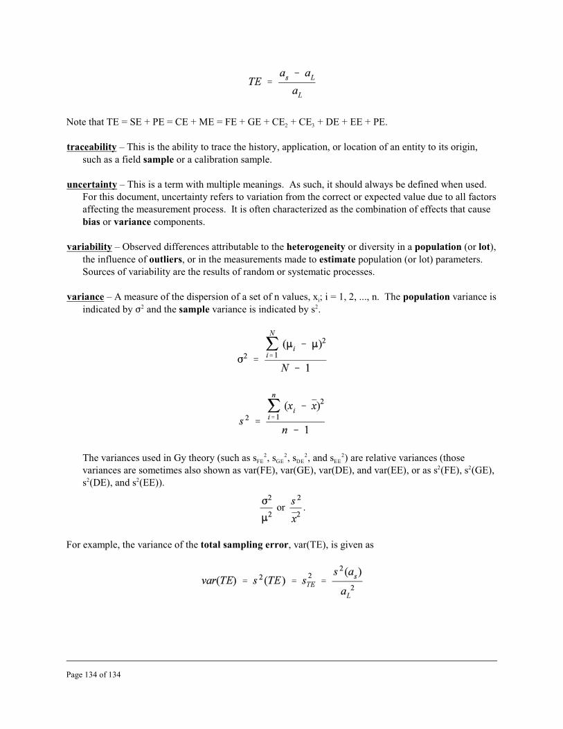
Note that TE = SE + PE = CE + ME = FE + GE + CE + CE + DE + EE + PE. 2 3

traceability – This is the ability to trace the history, application, or location of an entity to its origin, such as a field sample or a calibration sample.

uncertainty – This is a term with multiple meanings. As such, it should always be defined when used. For this document, uncertainty refers to variation from the correct or expected value due to all factors affecting the measurement process. It is often characterized as the combination of effects that cause bias or variance components.

variability – Observed differences attributable to the heterogeneity or diversity in a population (or lot), the influence of outliers, or in the measurements made to estimate population (or lot) parameters. Sources of variability are the results of random or systematic processes.

variance – A measure of the dispersion of a set of n values, x ; i = 1, 2, ..., n. The population variance is i2 2indicated by F and the sample variance is indicated by s .

2 2 2 2The variances used in Gy theory (such as sFE , sGE , s , and s ) are relative variances (those DE EE 2 2variances are sometimes also shown as var(FE), var(GE), var(DE), and var(EE), or as s (FE), s (GE),

2 2s (DE), and s (EE)).

or .

For example, the variance of the total sampling error, var(TE), is given as

Page 134 of 134