Embed Size (px)
DESCRIPTION
document
Citation preview
TESTS FOR UNEQUAL TREATMENT VARIANCES IN
CROSSOVER DESIGNS
by
YOONSUNG JUNG
B.S., Seowon University, Korea, 1995
M.S., Korea University, Korea, 1999
M.S., Texas A&M University, 2003
AN ABSTRACT OF A DISSERTATION
submitted in partial fulfillment of the
requirements for the degree
DOCTOR OF PHILOSOPHY
Department of Statistics
College of Arts and Sciences
KANSAS STATE UNIVERSITY
Manhattan, Kansas
2009
Abstract
A crossover design is an experimental design in which each experimental unit receives a
series of experimental treatments over time. The order that an experimental unit receives
its treatments is called a sequence (example, the sequence AB means that treatment A is
given first, and then followed by treatment B). A period is the time interval during which a
treatment is administered to the experimental unit. A period could range from a few minutes
to several months depending on the study. Sequences usually involve subjects receiving a
different treatment in each successive period. However, treatments may occur more than
once in any sequence (example, ABAB).
Treatments and periods are compared within subjects, i.e. each subject serves as his/her
own control. Therefore, any effect that is related to subject differences is removed from
treatment and period comparisons.
Carryover effects are residual effects from a previous treatment manifesting themselves
in subsequent periods. Crossover designs both with and without carryover are traditionally
analyzed assuming that the response due to different treatments have equal variances. The
effects of unequal variances on traditional tests for treatment and carryover difference were
recently considered in crossover designs assuming that the response due to treatments have
unequal variances with a compound symmetry correlation structure.
The likelihood function for the two treatment/two sequence crossover design has closed
form maximum likelihood solutions for the parameters at both the null hypothesis, H0 : σ2A =
σ2B, and at alternative hypothesis, HA : σ2
A 6= σ2B. Under HA : σ2
A 6= σ2B, the method of
moment estimators and the maximum likelihood estimators of σ2A, σ
2B and ρ are identi-
cal. The dual balanced design, ABA/BAB, which is balanced for carryover effects is also

considered. The dual balanced design has a closed form solution that maximizes the like-
lihood function under the null hypothesis, H0 : σ2A = σ2
B, but not for the alternative
hypothesis, HA : not H0. Similarly, the three treatment/three sequence crossover design,
ABC/BCA/CAB, has a closed form solution that maximizes the likelihood function at the
null hypothesis, H0 : σ2A = σ2
B = σ2C , but not for the alternative hypothesis, HA : not H0.
An iterative procedure is introduced to estimate the parameters for the two and three
treatment crossover designs. To check the performance of the likelihood ratio tests, Type I
error rates and power comparisons are explored using simulations.
TESTS FOR UNEQUAL TREATMENT VARIANCES IN
CROSSOVER DESIGNS
by
YOONSUNG JUNG
B.S., Seowon University, Korea, 1995
M.S., Korea University, Korea, 1999
M.S., Texas A&M University, 2003
A DISSERTATION
submitted in partial fulfillment of the
requirements for the degree
DOCTOR OF PHILOSOPHY
Department of Statistics
College of Arts and Sciences
KANSAS STATE UNIVERSITY
Manhattan, Kansas
2009
Approved by: Approved by:
Co-Major Professor Co-Major ProfessorDallas E. Johnson John E. Boyer, Jr.

Copyright
YOONSUNG JUNG
2009

Abstract
A crossover design is an experimental design in which each experimental unit receives a
series of experimental treatments over time. The order that an experimental unit receives
its treatments is called a sequence (example, the sequence AB means that treatment A is
given first, and then followed by treatment B). A period is the time interval during which a
treatment is administered to the experimental unit. A period could range from a few minutes
to several months depending on the study. Sequences usually involve subjects receiving a
different treatment in each successive period. However, treatments may occur more than
once in any sequence (example, ABAB).
Treatments and periods are compared within subjects, i.e. each subject serves as his/her
own control. Therefore, any effect that is related to subject differences is removed from
treatment and period comparisons.
Carryover effects are residual effects from a previous treatment manifesting themselves
in subsequent periods. Crossover designs both with and without carryover are traditionally
analyzed assuming that the response due to different treatments have equal variances. The
effects of unequal variances on traditional tests for treatment and carryover difference were
recently considered in crossover designs assuming that the response due to treatments have
unequal variances with a compound symmetry correlation structure.
The likelihood function for the two treatment/two sequence crossover design has closed
form maximum likelihood solutions for the parameters at both the null hypothesis, H0 : σ2A =
σ2B, and at alternative hypothesis, HA : σ2
A 6= σ2B. Under HA : σ2
A 6= σ2B, the method of
moment estimators and the maximum likelihood estimators of σ2A, σ
2B and ρ are identi-
cal. The dual balanced design, ABA/BAB, which is balanced for carryover effects is also

considered. The dual balanced design has a closed form solution that maximizes the like-
lihood function under the null hypothesis, H0 : σ2A = σ2
B, but not for the alternative
hypothesis, HA : not H0. Similarly, the three treatment/three sequence crossover design,
ABC/BCA/CAB, has a closed form solution that maximizes the likelihood function at the
null hypothesis, H0 : σ2A = σ2
B = σ2C , but not for the alternative hypothesis, HA : not H0.
An iterative procedure is introduced to estimate the parameters for the two and three
treatment crossover designs. To check the performance of the likelihood ratio tests, Type I
error rates and power comparisons are explored using simulations.
Table of Contents
Table of Contents viii
List of Figures x
List of Tables xi
Acknowledgements xiii
Preface xiv
1 Analysis of Crossover Designs When Treatments have Equal Variances 11.1 Introduction . . . . . . . . . . . . . . . . . . . . . . . . . . . . . . . . . . . . 11.2 Two Treatment/Two Sequence Crossover Design (AB/BA) . . . . . . . . . . 81.3 Three or More Treatments Crossover Design . . . . . . . . . . . . . . . . . . 15
2 Testing for Equal Treatment Variances in Two Treatment Crossover De-signs 212.1 Introduction . . . . . . . . . . . . . . . . . . . . . . . . . . . . . . . . . . . . 212.2 Testing the Equality of the Two Variances due to Treatments . . . . . . . . 262.3 A Simulation Study . . . . . . . . . . . . . . . . . . . . . . . . . . . . . . . . 322.4 Two Treatment/ Two sequence Crossover Design Balanced for Carryover Effect 38
2.4.1 Two Treatment/ Two Sequence Dual Balanced Design . . . . . . . . 382.4.2 Methods for Estimating Parameters . . . . . . . . . . . . . . . . . . . 46
2.5 Conclusions . . . . . . . . . . . . . . . . . . . . . . . . . . . . . . . . . . . . 492.6 Future Work . . . . . . . . . . . . . . . . . . . . . . . . . . . . . . . . . . . . 50
3 Testing for Equal Treatment Variances in a Three Treatment CrossoverDesign 513.1 Introduction . . . . . . . . . . . . . . . . . . . . . . . . . . . . . . . . . . . . 513.2 Testing the Equality of the Three Variances due to Treatments . . . . . . . . 553.3 Methods for Estimating Parameters . . . . . . . . . . . . . . . . . . . . . . . 613.4 A Simulation Study . . . . . . . . . . . . . . . . . . . . . . . . . . . . . . . . 643.5 Conclusions . . . . . . . . . . . . . . . . . . . . . . . . . . . . . . . . . . . . 703.6 Future Work . . . . . . . . . . . . . . . . . . . . . . . . . . . . . . . . . . . . 71
Bibliography 74
A Chapter 2: Figures for Two Treatment Crossover Design 75
viii

B Chapter 2: Tables for Two Treatment Crossover Design 79
C Chapter 3: Figures for Three Treatment Crossover Design 83
D Chapter 3: Tables for Three Treatment Crossover Design 90
E R Code 97
F SAS Code 114
ix

List of Figures
A.1 Type I Error Plot at (σ2A, σ
2B)=(1,1) . . . . . . . . . . . . . . . . . . . . . . . 76
A.2 Power Plot at (σ2A, σ
2B)=(1,2) . . . . . . . . . . . . . . . . . . . . . . . . . . 77
A.3 Power Plot at (σ2A, σ
2B)=(1,4) . . . . . . . . . . . . . . . . . . . . . . . . . . 77
A.4 Power Plot at (σ2A, σ
2B)=(1,8) . . . . . . . . . . . . . . . . . . . . . . . . . . 78
A.5 Power Plot at (σ2A, σ
2B)=(1,16) . . . . . . . . . . . . . . . . . . . . . . . . . . 78
C.1 Type I Error Plot at (σ2A, σ
2B, σ
2C)=(1,1,1) . . . . . . . . . . . . . . . . . . . . 84
C.2 Power Plot at (σ2A, σ
2B, σ
2C)=(1,1,2) . . . . . . . . . . . . . . . . . . . . . . . 85
C.3 Power Plot at (σ2A, σ
2B, σ
2C)=(1,1,4) . . . . . . . . . . . . . . . . . . . . . . . 85
C.4 Power Plot at (σ2A, σ
2B, σ
2C)=(1,1,8) . . . . . . . . . . . . . . . . . . . . . . . 86
C.5 Power Plot at (σ2A, σ
2B, σ
2C)=(1,1,16) . . . . . . . . . . . . . . . . . . . . . . . 86
C.6 Power Plot at (σ2A, σ
2B, σ
2C)=(2,2,1) . . . . . . . . . . . . . . . . . . . . . . . 87
C.7 Power Plot at (σ2A, σ
2B, σ
2C)=(4,4,1) . . . . . . . . . . . . . . . . . . . . . . . 87
C.8 Power Plot at (σ2A, σ
2B, σ
2C)=(8,8,1) . . . . . . . . . . . . . . . . . . . . . . . 88
C.9 Power Plot at (σ2A, σ
2B, σ
2C)=(16,16,1) . . . . . . . . . . . . . . . . . . . . . . 88
C.10 Power Plot at (σ2A, σ
2B, σ
2C)=(1,2,4) . . . . . . . . . . . . . . . . . . . . . . . 89
C.11 Power Plot at (σ2A, σ
2B, σ
2C)=(1,4,8) . . . . . . . . . . . . . . . . . . . . . . . 89
x

List of Tables
1.1 ANOVA Table for a Crossover Design Without Carryover Effects . . . . . . . 61.2 ANOVA Table for a Crossover Design With Carryover Effects . . . . . . . . 61.3 Two Treatment/Two Sequence Crossover Design (AB/BA) . . . . . . . . . . 71.4 Three Treatment/Three Sequence Crossover Design (ABC/BCA/CAB) . . . 71.5 Expected Cell Means for Model (1.1) . . . . . . . . . . . . . . . . . . . . . . 81.6 ANOVA Table for a Two Treatment/ Two Sequence Crossover Design With-
out Carryover Effects (AB/BA) . . . . . . . . . . . . . . . . . . . . . . . . . 91.7 Expected Cell Means for Model (1.2) . . . . . . . . . . . . . . . . . . . . . . 91.8 ANOVA Table for a Two Treatment/Two Sequence Crossover Design With
Carryover Effects (AB/BA) . . . . . . . . . . . . . . . . . . . . . . . . . . . 101.9 ANOVA Table for a Two Treatment/Two Sequence Crossover Design . . . . 121.10 Two Treatment/Two Sequence Crossover Design (ABA/BAB) . . . . . . . . 131.11 Two Treatment/Four Sequence Crossover Design (AB/BA/AA/BB) . . . . . 141.12 Three Treatment/Three Sequence Crossover Design (ABC/BCA/CAB) . . . 151.13 Expected Cell Means for a Three Treatment/Three Sequence Crossover De-
sign (ABC/BCA/CAB) for Model (1.1) . . . . . . . . . . . . . . . . . . . . . 161.14 ANOVA Table for Model (1.1) ANOVA Table for a Three Treatment/ Three
Sequence Crossover Design (ABC/BCA/CAB) Without Carryover Effects . . 161.15 Expected Cell Means for a Three Treatment/Three Sequence Crossover De-
sign (ABC/BCA/CAB) for Model (1.2) . . . . . . . . . . . . . . . . . . . . . 171.16 ANOVA Table for Model (1.2) ANOVA Table for a Three Treatment/Three
Sequence Crossover Design (ABC/BCA/CAB) With Carryover Effects . . . 181.17 A Three Treatment/Six Sequence Crossover Design (Two Latin Squares’ De-
sign: ABC/ACB/BAC/BCA/CAB/CBA) . . . . . . . . . . . . . . . . . . . 191.18 A Four Treatment/Four Sequence Crossover Design (One Latin Square De-
sign: ABDC/BCAD/CDBA/DACB) . . . . . . . . . . . . . . . . . . . . . . 19
2.1 Two Treatment/Two Sequence Crossover Design(AB/BA) . . . . . . . . . . 232.2 ANOVA Table for Model 2.1: Two Treatment/ Two Sequence Crossover De-
sign (AB/BA) Without Carryover Effects . . . . . . . . . . . . . . . . . . . . 242.3 Expected Cell Means for a Two Treatment/ Two Sequence Crossover Design
(AB/BA) for Model (2.1) . . . . . . . . . . . . . . . . . . . . . . . . . . . . . 252.4 ANOVA Table for Model 2.2: Two Treatment/Two Sequence Crossover De-
sign (AB/BA) With Carryover Effects . . . . . . . . . . . . . . . . . . . . . 252.5 Expected Cell Means for a Two Treatment/ Two Sequence Crossover Design
(AB/BA) for Model (2.2) . . . . . . . . . . . . . . . . . . . . . . . . . . . . . 25
xi

2.6 Parameter values used in Type I error rate and Power Analysis for the equalityof variances due to Treatment in a Two Treatment/ Two Sequence CrossoverDesign (AB/BA) for Model (2.1) . . . . . . . . . . . . . . . . . . . . . . . . 33
2.7 A Two Treatment/ Two Sequence Crossover Design with an Extra Period(ABA/BAB) . . . . . . . . . . . . . . . . . . . . . . . . . . . . . . . . . . . . 38
2.8 Expected Cell Means for a Two Treatment/ Two Sequence Crossover Designwith an Extra Period (ABA/BAB) for Model (2.2) . . . . . . . . . . . . . . 39
3.1 A Three Treatment/Three Sequence Crossover Design(ABC/BCA/CAB) . . 543.2 ANOVA Table for Model (3.1): a Three Treatment/ Three Sequence Crossover
Design (ABC/BCA/CAB) Without Carryover Effects . . . . . . . . . . . . . 543.3 ANOVA Table for Model (3.2): a Three Treatment/Three Sequence Crossover
Design (ABC/BCA/CAB) With Carryover Effects . . . . . . . . . . . . . . . 553.4 A Three Treatment/Six Sequence Crossover Design (Two Latin Squares’ De-
sign)(ABC/ACB/BAC/BCA/CAB/CBA) . . . . . . . . . . . . . . . . . . . 553.5 Setup of Parameters for Type I error rate and Power Analysis for the equal-
ity of variances due to Treatment at a Three Treatment/ Three SequenceCrossover Design (ABC/BCA/ CAB) for Model . . . . . . . . . . . . . . . . 65
B.1 Type I Error α = 0.05 at (σ2A, σ
2B)=(1,1) . . . . . . . . . . . . . . . . . . . . 80
B.2 Power at (σ2A, σ
2B)=(1,2) . . . . . . . . . . . . . . . . . . . . . . . . . . . . . 80
B.3 Power at (σ2A, σ
2B)=(1,4) . . . . . . . . . . . . . . . . . . . . . . . . . . . . . 81
B.4 Power at (σ2A, σ
2B)=(1,8) . . . . . . . . . . . . . . . . . . . . . . . . . . . . . 81
B.5 Power at (σ2A, σ
2B)=(1,16) . . . . . . . . . . . . . . . . . . . . . . . . . . . . . 82
D.1 Type I Error α = 0.05 at (σ2A, σ
2B, σ
2C)=(1,1,1) . . . . . . . . . . . . . . . . . 91
D.2 Power at (σ2A, σ
2B, σ
2C)=(1,1,2) . . . . . . . . . . . . . . . . . . . . . . . . . . 91
D.3 Power at (σ2A, σ
2B, σ
2C)=(1,1,4) . . . . . . . . . . . . . . . . . . . . . . . . . . 92
D.4 Power at (σ2A, σ
2B, σ
2C)=(1,1,8) . . . . . . . . . . . . . . . . . . . . . . . . . . 92
D.5 Power at (σ2A, σ
2B, σ
2C)=(1,1,16) . . . . . . . . . . . . . . . . . . . . . . . . . . 93
D.6 Power at (σ2A, σ
2B, σ
2C)=(2,2,1) . . . . . . . . . . . . . . . . . . . . . . . . . . 93
D.7 Power at (σ2A, σ
2B, σ
2C)=(4,4,1) . . . . . . . . . . . . . . . . . . . . . . . . . . 94
D.8 Power at (σ2A, σ
2B, σ
2C)=(8,8,1) . . . . . . . . . . . . . . . . . . . . . . . . . . 94
D.9 Power at (σ2A, σ
2B, σ
2C)=(16,16,1) . . . . . . . . . . . . . . . . . . . . . . . . . 95
D.10 Power at (σ2A, σ
2B, σ
2C)=(1,2,4) . . . . . . . . . . . . . . . . . . . . . . . . . . 95
D.11 Power at (σ2A, σ
2B, σ
2C)=(1,4,8) . . . . . . . . . . . . . . . . . . . . . . . . . . 96
xii

Acknowledgments
I would like to express my sincere thanks and appreciation to my major advisor, Dr.
Dallas E. Johnson for providing guidance, patience, understanding and support during the
course of this study. Also, I would like to thank Dr. John E. Boyer Jr. as a co-advisor
and committee member, I would like to thank the members of my graduate committee, Dr.
James J. Higgins and Dr. Carol W. Shanklin for reviewing my work and providing many
helpful comments.
I would like to thank the Department of Statistics for providing support during the
course of my studies.
I would like to thank my wife Ryunghee Kim and my son Andrew Jung for support
during the course of my study.
I would like to thank my parents, In-Chul Jeong and Ok-Young Yoon, parents-in-law,
Han-Soo Kim and Jung-Sook Cho, and my brothers and sisters for their love and support.
I would like to thank my mentor, Dr. Eunhee Kim, for her nice advice and support.
I would like to thank my god-parents, Raymond and Sun-Cha Felix for their love, prayers
and support.
Thank you so much to Meishusama.
xiii

Preface
A crossover design is an experimental design in which each experimental unit receives a
series of experimental treatments over time. The order that an experimental unit receives
its treatments is called a sequence (example, the sequence AB means that treatment A is
given first, and then followed by treatment B). A period is the time interval during which a
treatment is administered to the experimental unit. A period could range from a few minutes
to several months depending on the study. Sequences usually involve subjects receiving a
different treatment in each successive period. However, treatments may occur more than
once in any sequence (example, ABAB).
Treatments and periods are compared within subjects, i.e. each subject serves as his/her
own control. Therefore, any effect that is related to subject differences is removed from
treatment and period comparisons.
Carryover effects are residual effects from a previous treatment manifesting themselves
in subsequent periods. Crossover designs both with and without carryover are traditionally
analyzed assuming that the response due to treatments have equal variances. The effects of
unequal variances on traditional tests for the difference of treatment and carryover effects
were recently considered in crossover designs assuming that the responses due to treatments
have unequal variances with compound symmetry correlation structure.
Tests for the equality of variances due to treatments in crossover designs are considered
in this study.
xiv
Chapter 1
Analysis of Crossover Designs WhenTreatments have Equal Variances
1.1 Introduction
A crossover design is an experimental design in which each experimental unit receives a
series of experimental treatments over time. The order that an experimental unit receives
its treatments is called a sequence (example, the sequence AB means that treatment A is
given first, and then followed by treatment B). A period is the time interval during which a
treatment is administered to the experimental unit. A period could range from a few minutes
to several months depending on the study. Sequences usually involve subjects receiving a
different treatment in each successive period. However, treatments may occur more than
once in any sequence (example, ABAB).
Many crossover designs have been used in agriculture. Brant (1938)2 used a crossover
design for comparing two treatments using two groups of cattle. Fieller (1940)4 used a two
treatment/two sequence (AB/BA) crossover design with rabbits to compare the effects of
different doses of insulin in a biological assay. Crossover designs are also used in pharma-
ceutical studies where subjects with recurrent or chronic conditions, such as high blood
pressure, asthma, epilepsy, and angina, are being used to study different treatments. These
designs are suitable in situations where a patient(or a subject) is not cured by one of the
treatments during the course of the study. Grizzle (1965)9 describes some of the advantages
1

of crossover designs having two experimental periods.
In crossover trials, measurements on different treatments are taken from each subject
during or at the end of each period of treatment. Thus, treatments and periods are compared
within subjects, i.e. each subject serves as his/her own control. Therefore, any effects that
are related to subject differences are removed from treatment and period comparisons.
Crossover designs provide an advantage over parallel group designs (a separate group of
subjects for each treatment) because the standard error of a within subject contrast depends
on within subject variability in a crossover design rather than between subject variability
as in parallel group design. Within subject variability is usually much smaller than between
subject variability and allows for more precise estimates of treatment differences than can
be made using only between subject contrasts. A crossover design generally requires fewer
subjects than a design having a separate group of subjects for each treatment. The fewer
number of subjects makes crossover designs more economically viable. This is not possible
in a parallel groups design.
Crossover designs also have some disadvantages that should not be overlooked. In clinical
trials, patients may drop out of a study. Human subjects may tend to withdraw from a
study if they feel they are not gaining relief or benefit from one of the treatments. Patients
who drop out provide no direct information on the treatments they did not receive which
may make it difficult to analyze and interpret the data. Some diseases with a non-negligible
chance of death during the course of the trial are not suitable for crossover designs. Crossover
designs with long sequences of treatments may be inconvenient for patients. Subjects are
required to commit to a certain number of treatments and the total amount of time spent
may be too long for some studies. In crossover designs, treatments given in one period
may affect a treatment received in a subsequent period. Residual effects from a previous
treatment manifesting themselves in subsequent periods are called carryover effects and can
be either a prolonged or delayed response from a previous treatment. Carryover effects
that affect the nth period treatment are called nth order carryover effects (e.g. 1st and 2nd
2
order carryover effects affect the response of treatments applied 1 and 2 periods later). The
general view for carryover effects is that the effect of 2nd order carryover is much smaller
than that of a 1st order carryover effect. Crossover designs often incorporate a washout
period. A washout period is also called a rest period. It is a time during which subjects are
not given any of the treatments under investigation. It is hoped that the washout period
will eliminate or minimize possible carryover effects of a previous treatment in subsequent
periods. However, washout periods are not always feasible because, as a example, a patient
with a medical condition that requires continuous medical treatment may not allow for a
washout period. In an animal science study, animals may be put on different sequences of
feed rations to evaluate daily weight gain. In many of these cases, once the treatment is
changed, the researcher can leave the animal on the new treatment for a longer period of
time before collecting responses in order to minimize carryover effects.
Crossover designs are traditionally analyzed as a split-plot design. A split-plot design
has two different sizes of experimental units (whole plot and subplot experimental units).
The whole plot in a crossover design is the subject to which a sequence of treatments is
assigned and the subplot is the time interval (period). There are both between subject
comparisons and within subject comparisons in a crossover design. Treatment and period
effects are compared within subjects while sequence effects are compared between subjects.
Multivariate and mixed model analyses of crossover designs with more than two periods
were considered by Goad (1994)6. Goad considered a crossover experiment as a form of a
repeated measures experiment. An appropriate analysis of a repeated measures experiment
depends on the form of the variance-covariance matrix, Σ, of the repeated measures. Huynh
and Feldt (1970)12 defined type H structure of Σ and proved it to be a necessary and
sufficient condition for the within subject analysis of variance F -tests to be valid. In a
crossover experiment where Σ does not have type H structure and the analysis of variance
tests may not be valid, three alternative approaches were proposed by Goad. The first
approach approximates the distribution of the usual analysis of variance F -statistic with
3
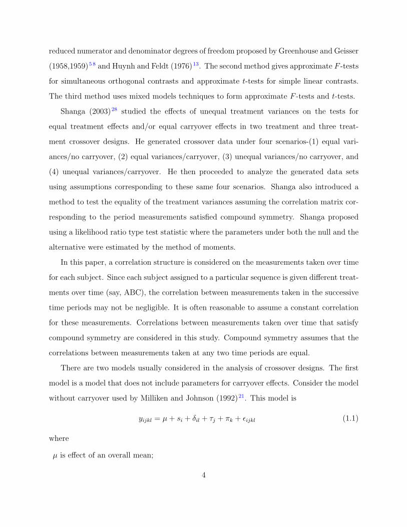
reduced numerator and denominator degrees of freedom proposed by Greenhouse and Geisser
(1958,1959)5 8 and Huynh and Feldt (1976)13. The second method gives approximate F -tests
for simultaneous orthogonal contrasts and approximate t-tests for simple linear contrasts.
The third method uses mixed models techniques to form approximate F -tests and t-tests.
Shanga (2003)28 studied the effects of unequal treatment variances on the tests for
equal treatment effects and/or equal carryover effects in two treatment and three treat-
ment crossover designs. He generated crossover data under four scenarios-(1) equal vari-
ances/no carryover, (2) equal variances/carryover, (3) unequal variances/no carryover, and
(4) unequal variances/carryover. He then proceeded to analyze the generated data sets
using assumptions corresponding to these same four scenarios. Shanga also introduced a
method to test the equality of the treatment variances assuming the correlation matrix cor-
responding to the period measurements satisfied compound symmetry. Shanga proposed
using a likelihood ratio type test statistic where the parameters under both the null and the
alternative were estimated by the method of moments.
In this paper, a correlation structure is considered on the measurements taken over time
for each subject. Since each subject assigned to a particular sequence is given different treat-
ments over time (say, ABC), the correlation between measurements taken in the successive
time periods may not be negligible. It is often reasonable to assume a constant correlation
for these measurements. Correlations between measurements taken over time that satisfy
compound symmetry are considered in this study. Compound symmetry assumes that the
correlations between measurements taken at any two time periods are equal.
There are two models usually considered in the analysis of crossover designs. The first
model is a model that does not include parameters for carryover effects. Consider the model
without carryover used by Milliken and Johnson (1992)21. This model is
yijkl = µ+ si + δil + τj + πk + εijkl (1.1)
where
µ is effect of an overall mean;
4

si is effect of the ith sequence effect, i = 1, 2, · · · , s;
δil is the experimental error associated with the lth subject in the ith sequence;
τj is effect of the jth treatment effect, j = 1, 2, · · · , t;
πk is effect of the kth period effect, k = 1, 2, · · · , p;
εijkl is the error associated with the lth subject in the ith sequence that received the jth
treatment in the kth period, l = 1, 2, · · · , ni.
δil ∼ iid N(0, σ2δ ) and εijkl ∼ iid N(0, σ2
ε ) for all i, j, k, and l.
all δil’s and εijkl’s are independent.
A second model includes parameters for carryover effects. The model for the response
variable may be written by modifying a notation used by Ratkowsky, Evan, and All-
dredge(1993)27. The model is
yijklm = µ+ si + δil + τj + πk + λm + εijklm (1.2)
where µ, si, τj, πk, and εijklm are defined as in (1.1)
λm is the carryover effect of the mth treatment administered in the previous period.
where m = 1, 2, · · · , t.
In both models the values for j and m are determined by the combination of i and k.
Also note that there is no carryover parameter associated with the first period. The general
form of an ANOVA table for crossover designs analyzed as a split-plot design for (1.1) is
given in Table 1.1.
5

Table 1.1: ANOVA Table for a Crossover Design Without Carryover Effects
Source dfBetween Subject AnalysisSequence s-1Subject(sequence) N-sWithin Subject AnalysisTreatment t-1Period p-1Error (N-1)(p-1)-(t-1)Total Np-1
The general form of an ANOVA table for crossover designs analyzed as a split-plot design
for (1.2) is given in Table 1.2.
Table 1.2: ANOVA Table for a Crossover Design With Carryover Effects
Source dfBetween Subject AnalysisSequence s-1Subject(sequence) N-sWithin Subject AnalysisTreatment t-1Period p-1Carryover t-1Error (N-1)(p-1)-2(t-1)Total Np-1
Let yil be the p × 1 vector of responses for the lth subject in the ith sequence and let
εil be the corresponding vector of random errors. Models (1.1) and (1.2) can be written as
yil = X iβ + εil, i = 1, 2, · · · , s; l = 1, 2, · · · , ni (1.3)
where β = (µ, s1, · · · , ss, τ1, · · · , τt, π1, · · · , πk)′ for model (1.1) and β = (µ, s1, · · · , ss, τ1, · · · , τt,
π1, · · · , πk, λ1, · · · , λt)′ for model (1.2). The elements in the design matrix X i depend
on the parameters associated with the ith sequence. In this paper, it is assumed that
εil ∼ iid N(0,Σi), i = 1, 2, · · · , s and l = 1, 2, · · · , ni.
6

Carryover effects present problems in the analysis of crossover designs. Sequence, treat-
ment, and period effects may be aliased with carryover effects. The problem of aliasing is
encountered in designs such as those in Tables 1.3 and 1.4.
Table 1.3: Two Treatment/Two Sequence Crossover Design (AB/BA)Period
Sequence 1 21 A B2 B A
Table 1.4: Three Treatment/Three Sequence Crossover Design (ABC/BCA/CAB)Period
Sequence 1 2 31 A B C2 B C A3 C A B
Consider the design in Table 1.4. Note that treatment B always follows treatment A
unless treatment B is given during period 1. Treatment A never follows treatment B. As
other patterns, treatment A always follows treatment C and treatment C always follows
treatment B. Therefore, if treatment C has a 1st order carryover effect, this will always
affect the outcome of treatment A, but it will never affect the outcome of treatment B.
This makes it impossible to distinguish the effect of treatment A from the carryover effect
of treatment C in this design. Therefore, we are interested in crossover designs balanced for
carryover effects where direct treatment comparisons can be made when carryover effects
exist.
The following sections consider the analysis of several different crossover designs.
7

1.2 Two Treatment/Two Sequence Crossover Design
(AB/BA)
The two treatment/two sequence crossover design is the simplest of all crossover designs.
It is also referred to as 2× 2 crossover design. In the 2× 2 crossover design, each treatment
is administered first in one sequence and last in the other sequence. AB is the order of
treatments A and B in the first sequence and BA is the order of the treatments in the
second sequence. Table 1.3 gives the sequences in a 2× 2 crossover design.
Consider the 2× 2 crossover design in Table 1.3. Under the assumptions on the random
effects given in (1.1), the covariance structure of the measurements on a subject in either
sequence 1 or 2 is
Σi = cov(yil) =
(σ2ε + σ2
δ σ2δ
σ2δ σ2
ε + σ2δ
), (1.4)
where i = 1, 2; l = 1, 2, · · · , ni.
The covariance matrices can also be reparameterized as
Σ1 = Σ2 = σ2
(1 ρρ 1
),
where
σ2 = σ2ε + σ2
δ and ρ =σ2δ
σ2ε + σ2
δ
.
Let µik be the expected response in the kth period of the ith sequence. Table 1.5 shows
expected cell means for model (1.1). Each cell mean is estimable if each cell is observed at
least once.
Table 1.5: Expected Cell Means for Model (1.1)Sequence Period
1 21 µ11 = µ+ s1 + τA + π1 µ12 = µ+ s1 + τB + π2
2 µ21 = µ+ s2 + τB + π1 µ22 = µ+ s2 + τA + π2
8

The general ANOVA table for the 2× 2 crossover design analyzed as a split-plot design
for (1.1) is given in Table 1.6 where ni equals the number of subjects assigned to the ith
sequence, i = 1, 2.
Table 1.6: ANOVA Table for a Two Treatment/ Two Sequence Crossover Design WithoutCarryover Effects (AB/BA)
Source dfBetween Subject AnalysisSequence 1Subject(sequence) (n1 + n2)-2Within Subject AnalysisTreatment 1Period 1Error (n1 + n2)-2Total 2(n1 + n2)-1
Table 1.7 shows the expected cell means for model (1.2).
Table 1.7: Expected Cell Means for Model (1.2)Sequence Period
1 21 µ11 = µ+ s1 + τA + π1 µ12 = µ+ s1 + τB + π2 + λA2 µ21 = µ+ s2 + τB + π1 µ22 = µ+ s2 + τA + π2 + λB
The general ANOVA table for the 2× 2 crossover design analyzed as a split-plot design
for (1.2) is given in Table 1.8.
9
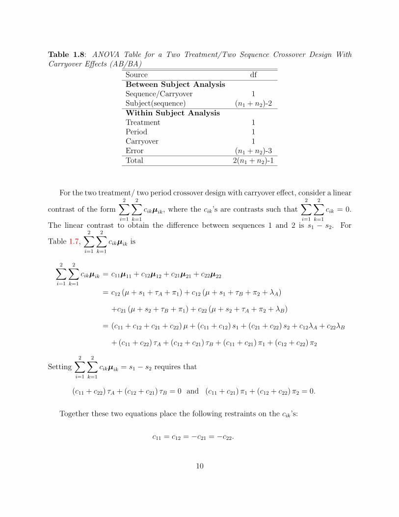
Table 1.8: ANOVA Table for a Two Treatment/Two Sequence Crossover Design WithCarryover Effects (AB/BA)
Source dfBetween Subject AnalysisSequence/Carryover 1Subject(sequence) (n1 + n2)-2Within Subject AnalysisTreatment 1Period 1Carryover 1Error (n1 + n2)-3Total 2(n1 + n2)-1
For the two treatment/ two period crossover design with carryover effect, consider a linear
contrast of the form2∑i=1
2∑k=1
cikµik, where the cik’s are contrasts such that2∑i=1
2∑k=1
cik = 0.
The linear contrast to obtain the difference between sequences 1 and 2 is s1 − s2. For
Table 1.7,2∑i=1
2∑k=1
cikµik is
2∑i=1
2∑k=1
cikµik = c11µ11 + c12µ12 + c21µ21 + c22µ22
= c12 (µ+ s1 + τA + π1) + c12 (µ+ s1 + τB + π2 + λA)
+c21 (µ+ s2 + τB + π1) + c22 (µ+ s2 + τA + π2 + λB)
= (c11 + c12 + c21 + c22)µ+ (c11 + c12) s1 + (c21 + c22) s2 + c12λA + c22λB
+ (c11 + c22) τA + (c12 + c21) τB + (c11 + c21) π1 + (c12 + c22) π2
Setting2∑i=1
2∑k=1
cikµik = s1 − s2 requires that
(c11 + c22) τA + (c12 + c21) τB = 0 and (c11 + c21) π1 + (c12 + c22) π2 = 0.
Together these two equations place the following restraints on the cik’s:
c11 = c12 = −c21 = −c22.
10
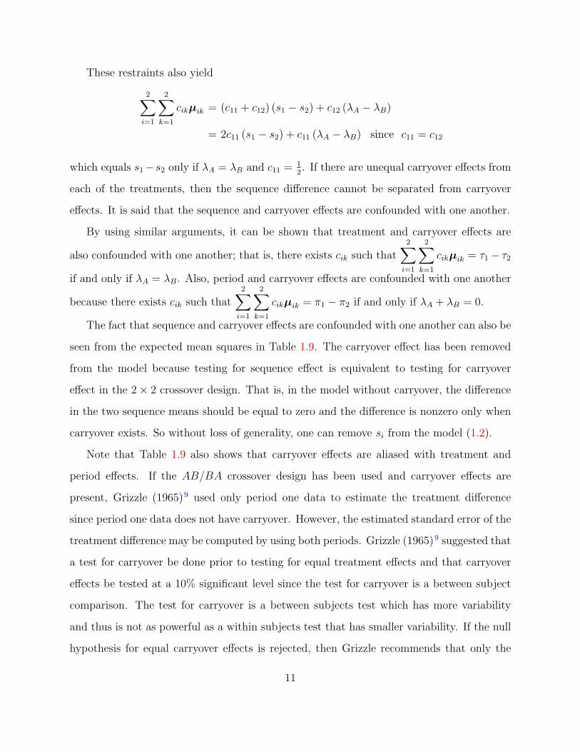
These restraints also yield
2∑i=1
2∑k=1
cikµik = (c11 + c12) (s1 − s2) + c12 (λA − λB)
= 2c11 (s1 − s2) + c11 (λA − λB) since c11 = c12
which equals s1−s2 only if λA = λB and c11 = 12. If there are unequal carryover effects from
each of the treatments, then the sequence difference cannot be separated from carryover
effects. It is said that the sequence and carryover effects are confounded with one another.
By using similar arguments, it can be shown that treatment and carryover effects are
also confounded with one another; that is, there exists cik such that2∑i=1
2∑k=1
cikµik = τ1− τ2
if and only if λA = λB. Also, period and carryover effects are confounded with one another
because there exists cik such that2∑i=1
2∑k=1
cikµik = π1 − π2 if and only if λA + λB = 0.
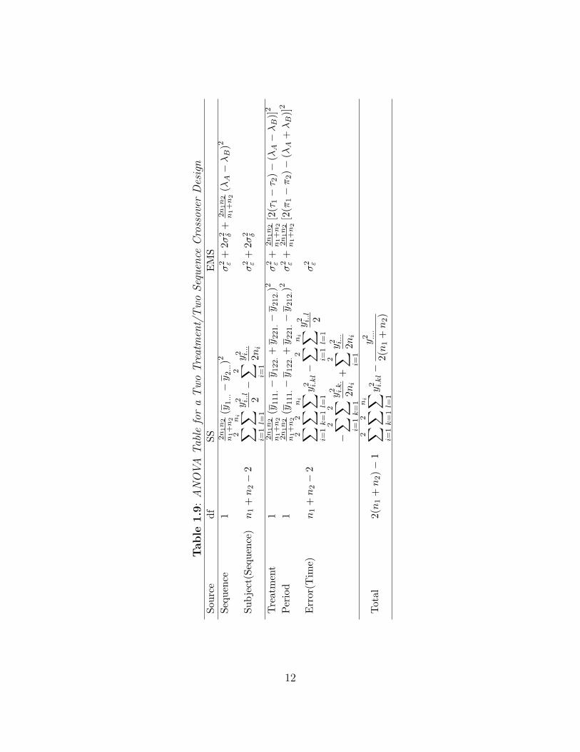
The fact that sequence and carryover effects are confounded with one another can also be
seen from the expected mean squares in Table 1.9. The carryover effect has been removed
from the model because testing for sequence effect is equivalent to testing for carryover
effect in the 2× 2 crossover design. That is, in the model without carryover, the difference
in the two sequence means should be equal to zero and the difference is nonzero only when
carryover exists. So without loss of generality, one can remove si from the model (1.2).
Note that Table 1.9 also shows that carryover effects are aliased with treatment and
period effects. If the AB/BA crossover design has been used and carryover effects are
present, Grizzle (1965)9 used only period one data to estimate the treatment difference
since period one data does not have carryover. However, the estimated standard error of the
treatment difference may be computed by using both periods. Grizzle (1965)9 suggested that
a test for carryover be done prior to testing for equal treatment effects and that carryover
effects be tested at a 10% significant level since the test for carryover is a between subject
comparison. The test for carryover is a between subjects test which has more variability
and thus is not as powerful as a within subjects test that has smaller variability. If the null
hypothesis for equal carryover effects is rejected, then Grizzle recommends that only the
11
Table
1.9
:A
NO
VA
Tab
lefo
ra
Tw
oT
reat
men
t/T
wo
Seq
uen
ceC
ross
over
Des
ign
Sour
cedf
SSE
MS
Sequ
ence
12n
1n
2n
1+n
2(y
1...−y
2...)
2σ
2 ε+
2σ2 δ
+2n
1n
2n
1+n
2(λA−λB
)2
Sub
ject
(Seq
uenc
e)n
1+n
2−
22 ∑ i=1
ni ∑ l=1
y2 i..l 2−
2 ∑ i=1
y2 i...
2ni
σ2 ε
+2σ
2 δ
Tre
atm
ent
12n
1n
2n
1+n
2(y
111.−y
122.+y
221.−y
212.)
2σ
2 ε+
2n
1n
2n
1+n
2[2
(τ1−τ 2
)−
(λA−λB
)]2
Per
iod
12n
1n
2n
1+n
2(y
111.−y
122.+y
221.−y
212.)
2σ
2 ε+
2n
1n
2n
1+n
2[2
(π1−π
2)−
(λA
+λB
)]2
Err
or(T
ime)
n1
+n
2−
22 ∑ i=1
2 ∑ k=
1
ni ∑ l=1
y2 i.kl−
2 ∑ i=1
ni ∑ l=1
y2 i..l 2
σ2 ε
−2 ∑ i=1
2 ∑ k=
1
y2 i.k.
2ni
+2 ∑ i=1
y2 i...
2ni
Tot
al2(n
1+n
2)−
12 ∑ i=1
2 ∑ k=
1
ni ∑ l=1
y2 i.kl−
y2 ....
2(n
1+n
2)
12

first period data be used for testing for equal treatment effects. If carryover effects are not
present in the model, then data from both periods can be used in testing for equal treatment
and equal period effects.
If a researcher knows that carryover effects will occur in a 2 × 2 crossover design, then
(s)he can consider some modifications to standard crossover designs to completely separate
treatment and carryover effects. The modification usually involves the addition of extra pe-
riods or extra sequences, or both. Two treatment crossover designs that avoid confounding
between treatment and carryover effects use an extra treatment period. Extra-period cross-
over designs are known as a dual balanced designs and were used by Patterson and Lucas
(1959)25 and Ratkowsky, Evans and Alldredge (1993)27. Dual balanced designs are designs
having a dual sequence in which the treatment order is reversed between the two sequences.
The construction of these designs simply involves repeating the treatments given to each
subject in the last period for one extra period, ABB and BAA. Treatment sequences given
by ABA/BAB is another example of a dual balanced design. The ABA/BAB design can be
combined with the ABB/BAA design to make the ABA/ABB/BAB/BAA design. Dual
balanced designs are able to make a comparison of treatment effects that is free from carry-
over using within subject contrasts even in the presence of carryover (Jones and Kenward,
2003)16.
Table 1.10 shows the ABA/BAB crossover design.
Table 1.10: Two Treatment/Two Sequence Crossover Design (ABA/BAB)Period
Sequence 1 2 31 A B A2 B A B
Under the assumptions given in (1.2), the variance-covariance matrices for the two se-
quences in the two treatment/two period design are given by
Σ1 = Σ2 = σ2
(1 ρρ 1
)13
where
σ2 = σ2δ + σ2
ε and ρ =σ2ε
σ2δ + σ2
ε
.
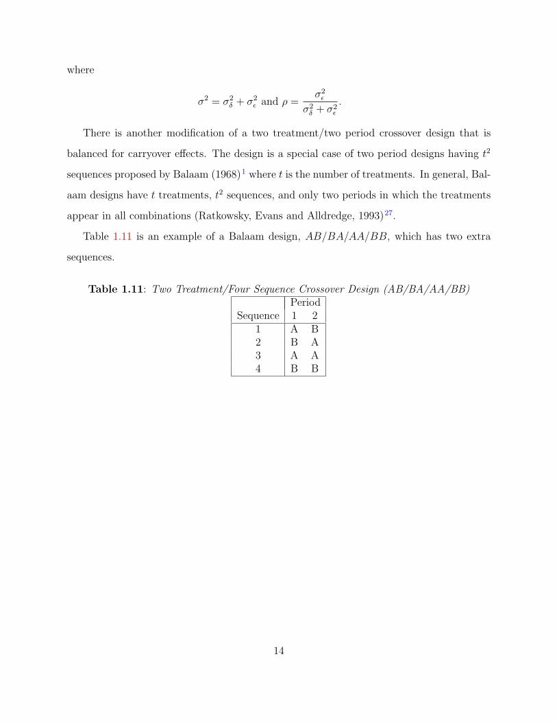
There is another modification of a two treatment/two period crossover design that is
balanced for carryover effects. The design is a special case of two period designs having t2
sequences proposed by Balaam (1968)1 where t is the number of treatments. In general, Bal-
aam designs have t treatments, t2 sequences, and only two periods in which the treatments
appear in all combinations (Ratkowsky, Evans and Alldredge, 1993)27.
Table 1.11 is an example of a Balaam design, AB/BA/AA/BB, which has two extra
sequences.
Table 1.11: Two Treatment/Four Sequence Crossover Design (AB/BA/AA/BB)Period
Sequence 1 21 A B2 B A3 A A4 B B
14

1.3 Three or More Treatments Crossover Design
This section considers crossover designs with three or more treatments. Table 1.12 shows
a basic cyclic three treatment/ three sequence crossover design.
Table 1.12: Three Treatment/Three Sequence Crossover Design (ABC/BCA/CAB)Period
Sequence 1 2 31 A B C2 B C A3 C A B
Under the assumptions on the random effects given in (1.1), the covariance structure of
the measurements on a subject in each sequence is
Σi = cov(yil) =
σ2ε + σ2
δ σ2δ σ2
δ
σ2δ σ2
ε + σ2δ σ2
δ
σ2δ σ2
δ σ2ε + σ2
δ
, (1.5)
where i = 1, 2, 3; l = 1, 2, · · · , ni.
It is also reparameterized by
Σ1 = Σ2 = Σ3 = σ2
1 ρ ρρ 1 ρρ ρ 1
where
σ2 = σ2ε + σ2
δ and ρ =σ2δ
σ2ε + σ2
δ
.
Let µik be the expected response in the kth period of the ith sequence. Table 1.13 shows
the expected cell means for model (1.1). Each cell mean is estimable if there is at least one
observation in each of the cells.
15

Table 1.13: Expected Cell Means for a Three Treatment/Three Sequence Crossover Design(ABC/BCA/CAB) for Model (1.1)
Sequence Period1 2 3
1 µ11 = µ+ s1 + τA + π1 µ12 = µ+ s1 + τB + π2 µ13 = µ+ s1 + τC + π3
2 µ21 = µ+ s2 + τB + π1 µ22 = µ+ s2 + τC + π2 µ23 = µ+ s2 + τA + π3
3 µ31 = µ+ s3 + τC + π1 µ32 = µ+ s3 + τA + π2 µ33 = µ+ s3 + τB + π3
The general ANOVA table for the three treatment/ three sequence crossover design
analyzed as a split-plot design for model (1.1) is given in Table 1.14 where ni equals the
number of subjects assigned to the ith sequence, i = 1, 2, 3.
Table 1.14: ANOVA Table for Model (1.1) ANOVA Table for a Three Treatment/ ThreeSequence Crossover Design (ABC/BCA/CAB) Without Carryover Effects
Source dfBetween Subject Analysis
Sequence 2Subject(sequence) (n1 + n2 + n3)-3Within Subject Analysis
Treatment 2Period 2Error 2(n1 + n2 + n3)-4Total 3(n1 + n2 + n3)-1
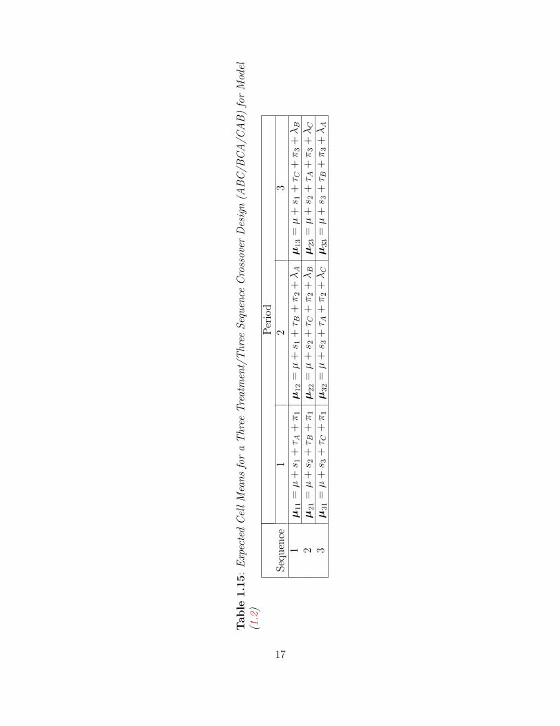
The analysis in Table 1.14 is valid only when there are no carryover effects. The expected
cell means for model (1.2) are given in Table 1.15.
16
Table
1.1
5:
Exp
ecte
dC
ell
Mea
ns
for
aT
hree
Tre
atm
ent/
Thr
eeS
equ
ence
Cro
ssov
erD
esig
n(A
BC
/BC
A/C
AB
)fo
rM
odel
(1.2
)P
erio
dSeq
uen
ce1
23
1µ
11
=µ
+s 1
+τ A
+π
1µ
12
=µ
+s 1
+τ B
+π
2+λA
µ13
=µ
+s 1
+τ C
+π
3+λB
2µ
21
=µ
+s 2
+τ B
+π
1µ
22
=µ
+s 2
+τ C
+π
2+λB
µ23
=µ
+s 2
+τ A
+π
3+λC
3µ
31
=µ
+s 3
+τ C
+π
1µ
32
=µ
+s 3
+τ A
+π
2+λC
µ33
=µ
+s 3
+τ B
+π
3+λA
17
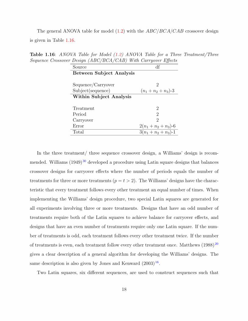
The general ANOVA table for model (1.2) with the ABC/BCA/CAB crossover design
is given in Table 1.16.
Table 1.16: ANOVA Table for Model (1.2) ANOVA Table for a Three Treatment/ThreeSequence Crossover Design (ABC/BCA/CAB) With Carryover Effects
Source dfBetween Subject Analysis
Sequence/Carryover 2Subject(sequence) (n1 + n2 + n3)-3Within Subject Analysis
Treatment 2Period 2Carryover 2Error 2(n1 + n2 + n3)-6Total 3(n1 + n2 + n3)-1
In the three treatment/ three sequence crossover design, a Williams’ design is recom-
mended. Williams (1949)30 developed a procedure using Latin square designs that balances
crossover designs for carryover effects where the number of periods equals the number of
treatments for three or more treatments (p = t > 2). The Williams’ designs have the charac-
teristic that every treatment follows every other treatment an equal number of times. When
implementing the Williams’ design procedure, two special Latin squares are generated for
all experiments involving three or more treatments. Designs that have an odd number of
treatments require both of the Latin squares to achieve balance for carryover effects, and
designs that have an even number of treatments require only one Latin square. If the num-
ber of treatments is odd, each treatment follows every other treatment twice. If the number
of treatments is even, each treatment follow every other treatment once. Matthews (1988)20
gives a clear description of a general algorithm for developing the Williams’ designs. The
same description is also given by Jones and Kenward (2003)16.
Two Latin squares, six different sequences, are used to construct sequences such that
18
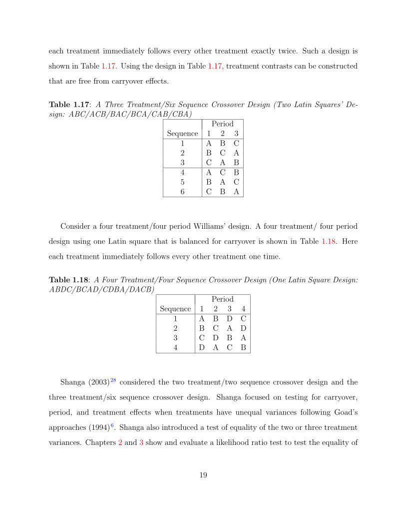
each treatment immediately follows every other treatment exactly twice. Such a design is
shown in Table 1.17. Using the design in Table 1.17, treatment contrasts can be constructed
that are free from carryover effects.
Table 1.17: A Three Treatment/Six Sequence Crossover Design (Two Latin Squares’ De-sign: ABC/ACB/BAC/BCA/CAB/CBA)
PeriodSequence 1 2 3
1 A B C2 B C A3 C A B4 A C B5 B A C6 C B A
Consider a four treatment/four period Williams’ design. A four treatment/ four period
design using one Latin square that is balanced for carryover is shown in Table 1.18. Here
each treatment immediately follows every other treatment one time.
Table 1.18: A Four Treatment/Four Sequence Crossover Design (One Latin Square Design:ABDC/BCAD/CDBA/DACB)
PeriodSequence 1 2 3 4
1 A B D C2 B C A D3 C D B A4 D A C B
Shanga (2003)28 considered the two treatment/two sequence crossover design and the
three treatment/six sequence crossover design. Shanga focused on testing for carryover,
period, and treatment effects when treatments have unequal variances following Goad’s
approaches (1994)6. Shanga also introduced a test of equality of the two or three treatment
variances. Chapters 2 and 3 show and evaluate a likelihood ratio test to test the equality of
19

variances when there are two or three treatments. The properties of these likelihood ratio
tests are explored using simulations.
20
Chapter 2
Testing for Equal TreatmentVariances in Two TreatmentCrossover Designs
2.1 Introduction
A crossover design is an experimental design in which each experimental unit receives a
series of experimental treatments over time. The order that an experimental unit receives
its treatments is called a sequence (example, the sequence ABC means that treatment A
is given first, and then followed by treatment B, then followed by treatment C). A period
is the time interval during which a treatment is administered to the experimental unit. A
period could range from a few minutes to several months depending on the study. Sequences
usually involve subjects receiving a different treatment in each successive period. However,
treatments may occur more than once in any sequence (example, ABAB).
A two treatment/two sequence crossover design (AB/BA) is the simplest of all crossover
designs. It is referred to as a 2×2 crossover design. In the 2×2 crossover design, AB is the
order of the treatments A and B in the first sequence and BA is the order of the treatments
B and A in the second sequence. Other two treatment designs can be formed by adding
extra period(s) and/or sequence(s) to the 2× 2 crossover design. ABA/BAB is an example
of an extra period crossover design known as a dual balanced design. AB/BA/AA/BB is
an example of an extra sequence crossover design known as a Balaam design.
21

Consider the 2×2 crossover design given in Table 2.1, and suppose there are n1 subjects
assigned to the AB sequence and n2 subjects assigned to the BA sequence. There are two
models usually considered in the traditional analysis of crossover designs. The first model is
a model that does not include parameters for carryover effects. Consider the model without
carryover used by Milliken and Johnson (1992)21. This model is
yijkl = µ+ si + δil + τj + πk + εijkl (2.1)
where
µ is effect of an overall mean;
si is effect of the ith sequence effect, i = 1, 2, · · · , s;
δil is the experimental error associated with the lth subject in the ith sequence;
τj is effect of the jth treatment effect, j = 1, 2, · · · , t;
πk is effect of the kth period effect, k = 1, 2, · · · , p;
εijkl is the error associated with the lth subject in the ith sequence that received the jthtreatment in the kth period, l = 1, 2, · · · , ni.
Also, it is often assumed that δil ∼ iid N(0, σ2δ ) and εijkl ∼ iid N(0, σ2
ε ) for all i, j, k,
and l. Finally, it is usually assumed that all δil’s and εijkl’s are independent. The value of
j is determined by i and k.
A second model includes parameters for carryover effects. The model for the response
variable may be written by modifying a notation used by Ratkowsky, Evan, and All-
dredge(1993)27. The model is
yijklm = µ+ si + δil + τj + πk + λm + εijklm (2.2)
where µ, si, τj, πk, and εijklm are defined as in (2.1) above, and λm is the carryover effect of
the mth treatment administered in the previous period, where m = 1, 2, · · · , t. There is no
carryover parameter associated with the first period.
22
Let yil be the p× 1 vector of responses for the lth subject in the ith sequence and let εil
be the corresponding vector of random errors. Models (2.1) and (2.2) can be written as
yil = X iβ + εil, i = 1, 2, · · · , s; l = 1, 2, · · · , ni (2.3)
where β = (µ, s1, · · · , ss, τ1, · · · , τt, π1, · · · , πk)′ for model (2.1) and β = (µ, s1, · · · , ss, τ1, · · · ,
τt, π1, · · · , πk, λ1, · · · , λt)′ for model (2.2). The elements in the design matrix X i depend
on the sequence of treatments in the ith sequence. In this paper, it is assumed that
εil ∼ iid N(0,Σ), i = 1, 2, · · · , s and l = 1, 2, · · · , ni.
Consider a two treatment/two period crossover design (AB/BA) with s = 2 in (2.3).
Under the assumptions on the random effects given in (2.1), the covariance structure of the
measurements on a subject in either sequence 1 or sequence 2 is
Σ = cov(yil) =
(σ2ε + σ2
δ σ2δ
σ2δ σ2
ε + σ2δ
), i = 1, 2; l = 1, 2, · · · , ni. (2.4)
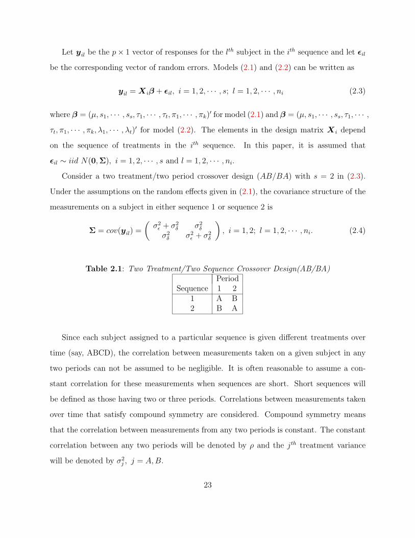
Table 2.1: Two Treatment/Two Sequence Crossover Design(AB/BA)Period
Sequence 1 21 A B2 B A
Since each subject assigned to a particular sequence is given different treatments over
time (say, ABCD), the correlation between measurements taken on a given subject in any
two periods can not be assumed to be negligible. It is often reasonable to assume a con-
stant correlation for these measurements when sequences are short. Short sequences will
be defined as those having two or three periods. Correlations between measurements taken
over time that satisfy compound symmetry are considered. Compound symmetry means
that the correlation between measurements from any two periods is constant. The constant
correlation between any two periods will be denoted by ρ and the jth treatment variance
will be denoted by σ2j , j = A,B.
23
Using the preceding assumptions, the correlation matrix for the 2 × 2 crossover design
will be denoted by R and R =
(1 ρρ 1
). The correlation between period measurements
together with the unequal variances due to the two treatments yield variance-covariance
matrices for sequences 1 and 2, respectively, as
Σ1 = cov(y1l) =
(σ2A ρσAσB
ρσAσB σ2B
)and
Σ2 = cov(y2l) =
(σ2B ρσAσB
ρσAσB σ2A
)(2.5)
where σ2A and σ2
B are variances due to treatments A and B, respectively, and ρ is the
correlation between observations in periods 1 and 2 for the same subject. If σ2A = σ2
B = σ2,
then cov(yil) = σ2
(1 ρρ 1
)for i = 1, 2 and l = 1, 2, · · · , ni. This covariance structure is
equivalent to the one given in (2.4) with σ2 = σ2ε + σ2
δ and ρ =σ2δ
σ2ε+σ
2δ.
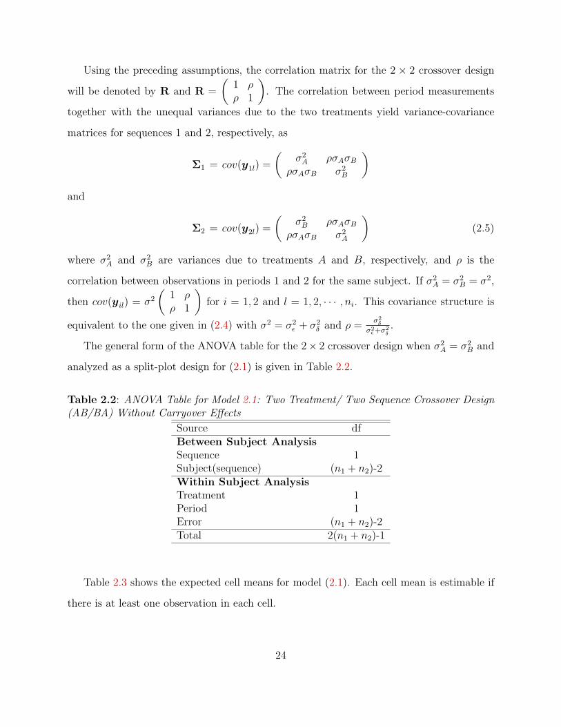
The general form of the ANOVA table for the 2× 2 crossover design when σ2A = σ2
B and
analyzed as a split-plot design for (2.1) is given in Table 2.2.
Table 2.2: ANOVA Table for Model 2.1: Two Treatment/ Two Sequence Crossover Design(AB/BA) Without Carryover Effects
Source dfBetween Subject AnalysisSequence 1Subject(sequence) (n1 + n2)-2Within Subject AnalysisTreatment 1Period 1Error (n1 + n2)-2Total 2(n1 + n2)-1
Table 2.3 shows the expected cell means for model (2.1). Each cell mean is estimable if
there is at least one observation in each cell.
24
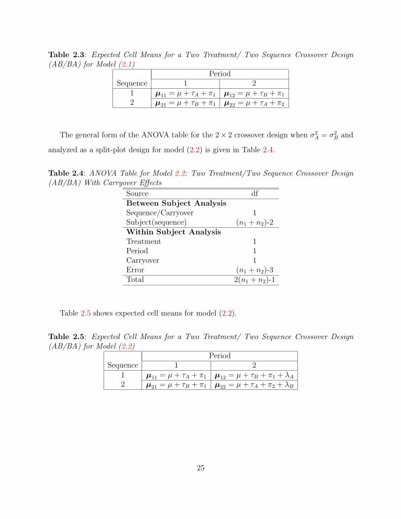
Table 2.3: Expected Cell Means for a Two Treatment/ Two Sequence Crossover Design(AB/BA) for Model (2.1)
PeriodSequence 1 2
1 µ11 = µ+ τA + π1 µ12 = µ+ τB + π1
2 µ21 = µ+ τB + π1 µ22 = µ+ τA + π2
The general form of the ANOVA table for the 2× 2 crossover design when σ2A = σ2
B and
analyzed as a split-plot design for model (2.2) is given in Table 2.4.
Table 2.4: ANOVA Table for Model 2.2: Two Treatment/Two Sequence Crossover Design(AB/BA) With Carryover Effects
Source dfBetween Subject AnalysisSequence/Carryover 1Subject(sequence) (n1 + n2)-2Within Subject AnalysisTreatment 1Period 1Carryover 1Error (n1 + n2)-3Total 2(n1 + n2)-1
Table 2.5 shows expected cell means for model (2.2).
Table 2.5: Expected Cell Means for a Two Treatment/ Two Sequence Crossover Design(AB/BA) for Model (2.2)
PeriodSequence 1 2
1 µ11 = µ+ τA + π1 µ12 = µ+ τB + π1 + λA2 µ21 = µ+ τB + π1 µ22 = µ+ τA + π2 + λB
25
2.2 Testing the Equality of the Two Variances due to
Treatments
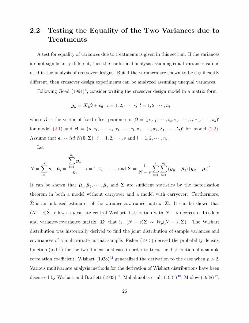
A test for equality of variances due to treatments is given in this section. If the variances
are not significantly different, then the traditional analysis assuming equal variances can be
used in the analysis of crossover designs. But if the variances are shown to be significantly
different, then crossover design experiments can be analyzed assuming unequal variances.
Following Goad (1994)6, consider writing the crossover design model in a matrix form
yil = X iβ + εil, i = 1, 2, · · · , s; l = 1, 2, · · · , ni
where β is the vector of fixed effect parameters; β = (µ, s1, · · · , ss, τ1, · · · , τt, π1, · · · , πk)′
for model (2.1) and β = (µ, s1, · · · , ss, τ1, · · · , τt, π1, · · · , πk, λ1, · · · , λt)′ for model (2.2).
Assume that εil ∼ iid N(0,Σ), i = 1, 2, · · · , s and l = 1, 2, · · · , ni.
Let
N =s∑i=1
ni, µi =
ni∑l=1
yil
ni, i = 1, 2, · · · , s, and Σ =
1
N − s
s∑i=1
ni∑l=1
(yil − µi) (yil − µi)′ .
It can be shown that µ1, µ2, · · · , µs and Σ are sufficient statistics by the factorization
theorem in both a model without carryover and a model with carryover. Furthermore,
Σ is an unbiased estimator of the variance-covariance matrix, Σ. It can be shown that
(N − s)Σ follows a p-variate central Wishart distribution with N − s degrees of freedom
and variance-covariance matrix, Σ; that is, (N − s)Σ ∼ Wp(N − s,Σ). The Wishart
distribution was historically derived to find the joint distribution of sample variances and
covariances of a multivariate normal sample. Fisher (1915) derived the probability density
function (p.d.f.) for the two dimensional case in order to treat the distribution of a sample
correlation coefficient. Wishart (1928)31 generalized the derivation to the case when p > 2.
Various multivariate analysis methods for the derivation of Wishart distributions have been
discussed by Wishart and Bartlett (1933)32, Mahalanobis et al. (1937)18, Madow (1938)17,
26
Hsu (1939)10, Elfving (1947)3, Sverdrup (1947)29, Rasch (1948)26, Ogawa (1953)24, Olkin
and Roy (1954)23, James (1954)15, and Jambunathan (1965)14. The Wishart distribution
is a multivariate generalization of the chi-squared distribution.
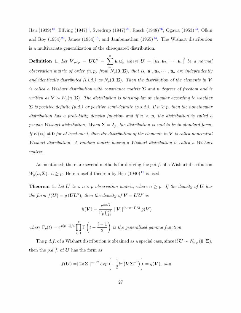
Definition 1. Let V p×p = UU ′ =n∑i=1
uiu′i, where U = [u1,u2, · · · ,un]′ be a normal
observation matrix of order (n, p) from Np(0,Σ); that is, u1,u2, · · · ,un are independently
and identically distributed (i.i.d.) as Np(0,Σ). Then the distribution of the elements in V
is called a Wishart distribution with covariance matrix Σ and n degrees of freedom and is
written as V ∼ Wp(n,Σ). The distribution is nonsingular or singular according to whether
Σ is positive definite (p.d.) or positive semi-definite (p.s.d.). If n ≥ p, then the nonsingular
distribution has a probability density function and if n < p, the distribution is called a
pseudo Wishart distribution. When Σ = Ip, the distribution is said to be in standard form.
If E (ui) 6= 0 for at least one i, then the distribution of the elements in V is called noncentral
Wishart distribution. A random matrix having a Wishart distribution is called a Wishart
matrix.
As mentioned, there are several methods for deriving the p.d.f. of a Wishart distribution
Wp(n,Σ), n ≥ p. Here a useful theorem by Hsu (1940)11 is used.
Theorem 1. Let U be a n × p observation matrix, where n ≥ p. If the density of U has
the form f(U ) = g (UU ′), then the density of V = UU ′ is
h(V ) =πnp/2
Γp(n2
) | V |(n−p−1)/2 g(V )
where Γp(t) = πp(p−1)/4
p∏i=1
Γ
(t− i− 1
2
)is the generalized gamma function.
The p.d.f. of a Wishart distribution is obtained as a special case, since ifU ∼ Nn,p (0,Σ),
then the p.d.f. of U has the form as
f(U) =| 2πΣ |−n/2 exp{−1
2tr(V Σ−1
)}= g(V ), say.
27
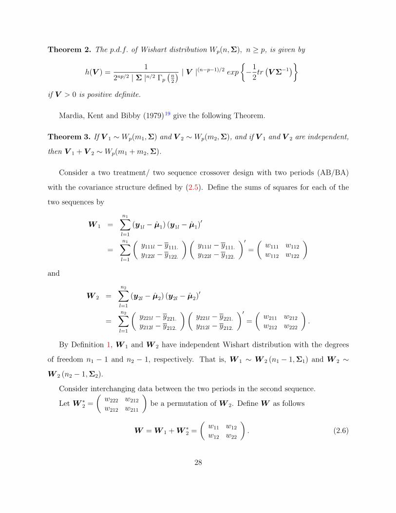
Theorem 2. The p.d.f. of Wishart distribution Wp(n,Σ), n ≥ p, is given by
h(V ) =1
2np/2 | Σ |n/2 Γp(n2
) | V |(n−p−1)/2 exp
{−1
2tr(V Σ−1
)}if V > 0 is positive definite.
Mardia, Kent and Bibby (1979)19 give the following Theorem.
Theorem 3. If V 1 ∼ Wp(m1,Σ) and V 2 ∼ Wp(m2,Σ), and if V 1 and V 2 are independent,
then V 1 + V 2 ∼ Wp(m1 +m2,Σ).
Consider a two treatment/ two sequence crossover design with two periods (AB/BA)
with the covariance structure defined by (2.5). Define the sums of squares for each of the
two sequences by
W 1 =
n1∑l=1
(y1l − µ1) (y1l − µ1)′
=
n1∑l=1
(y111l − y111.
y122l − y122.
)(y111l − y111.
y122l − y122.
)′=
(w111 w112
w112 w122
)and
W 2 =
n2∑l=1
(y2l − µ2) (y2l − µ2)′
=
n2∑l=1
(y221l − y221.
y212l − y212.
)(y221l − y221.
y212l − y212.
)′=
(w211 w212
w212 w222
).
By Definition 1, W 1 and W 2 have independent Wishart distribution with the degrees
of freedom n1 − 1 and n2 − 1, respectively. That is, W 1 ∼ W 2 (n1 − 1,Σ1) and W 2 ∼
W 2 (n2 − 1,Σ2).
Consider interchanging data between the two periods in the second sequence.
Let W ∗2 =
(w222 w212
w212 w211
)be a permutation of W 2. Define W as follows
W = W 1 +W ∗2 =
(w11 w12
w12 w22
). (2.6)
28

Then, by Theorem 3, W has a Wishart distribution with n1 +n2− 2 degrees of freedom
and variance-covariance structure Σ where Σ =
(σ2A ρσAσB
ρσAσB σ2B
)= D1/2RD1/2 where
D1/2 = diag(σA, σB) and R =
(1 ρρ 1
).
The inverse of Σ is given by
Σ−1 = D−1/2R−1D−1/2
where D−1/2 = diag(
1σA, 1σB
)and R−1 = 1
1−ρ2
(1 −ρ−ρ 1
).
One can get estimates of σ2A, σ
2B and ρ by the method of moments (MM).
Consider E(
1N−2
W)
= Σ =
(σ2A ρσAσB
ρσAσB σ2B
). Then the method of moments esti-
mates of σ2A, σ
2B and ρ are
σ2A =
w11
N − 2, σ2
B =w22
N − 2, ρ =
w12√w11w22
where N = n1 + n2.
Now consider testing H0 : σ2A = σ2
B versus HA : σ2A 6= σ2
B.
A likelihood function based on W is given by
L(Σ) = c|W |N−5
2 exp(−1
2tr(WΣ−1
))|Σ|N−2
2
where c =1
2N−2π1/2
2∏i=1
Γ
(N − i− 1
2
) .The log-likelihood function is
logL(Σ) = log(c) +N − 5
2log|W | − N − 2
2log|Σ| − 1
2tr(WΣ−1
).
Under H0 : σ2A = σ2
B = σ2,
|Σ| =(1− ρ2
)σ4 and tr
(WΣ−1
)=w11 + w22 − 2ρw12
(1− ρ2)σ2.
Therefore, the log-likelihood function is
logL(Σ) = log(c) +N − 5
2log|W | − (N − 2)log
(σ2)− N − 2
2log(1− ρ2
)−w11 + w22 − 2ρw12
2 (1− ρ2)σ2.
29

The derivatives of logL(Σ) with respect to σ2 and ρ are
∂logL(Σ)
∂σ2= −N − 2
σ2+w11 + w22 − 2ρw12
2 (1− ρ2)σ4
∂logL(Σ)
∂ρ=
(N − 2)ρ
1− ρ2+w12 (1− ρ2)− ρ(w11 + w22 − 2ρw12)
(1− ρ2)2 σ2.
Setting the derivatives of logL(Σ) with respect to σ2 and ρ equal to zero, one gets
−2(N − 2)σ2 +w11 + w22 − 2ρw12
(1− ρ2)= 0
(N − 2)ρ(1− ρ2
)+w12 (1− ρ2)− ρ(w11 + w22 − 2ρw12)
σ2= 0.
Then, under H0 : σ2A = σ2
B = σ2, the maximum likelihood estimators of σ2 and ρ are
σ2R =
w11 + w22 − 2ρRw12
2(N − 2) (1− ρ2R)
and ρR =2w12
w11 + w22
, respectively.
Under HA : σ2A 6= σ2
B,
|Σ| =(1− ρ2
)σ2Aσ
2B and tr
(WΣ−1
)=
1
1− ρ2
[w11
σ2A
+w22
σ2B
− 2ρw12
σAσB
].
Therefore the log-likelihood function is
logL(Σ) = log(c) +N − 5
2log|W | − N − 2
2log(σ2A
)− N − 2
2log(σ2B
)−N − 2
2log(1− ρ2
)− 1
2 (1− ρ2)
[w11
σ2A
+w22
σ2B
− 2ρw12
σAσB
].
The derivatives of logL(Σ) with respect to σ2A, σ
2B, and ρ are
∂logL(Σ)
∂σ2A
= −N − 2
2σ2A
+w11
2 (1− ρ2)σ4A
− ρw12
2 (1− ρ2)σ3AσB
,
∂logL(Σ)
∂σ2B
= −N − 2
2σ2B
+w22
2 (1− ρ2)σ4B
− ρw12
2 (1− ρ2)σAσ3B
, (2.7)
∂logL(Σ)
∂ρ=
(N − 2)ρ
1− ρ2− ρ
(1− ρ2)2
[w11
σ2A
+w22
σ2B
− ρw12
σAσB
]+
w12
(1− ρ2)2 σAσB.
30
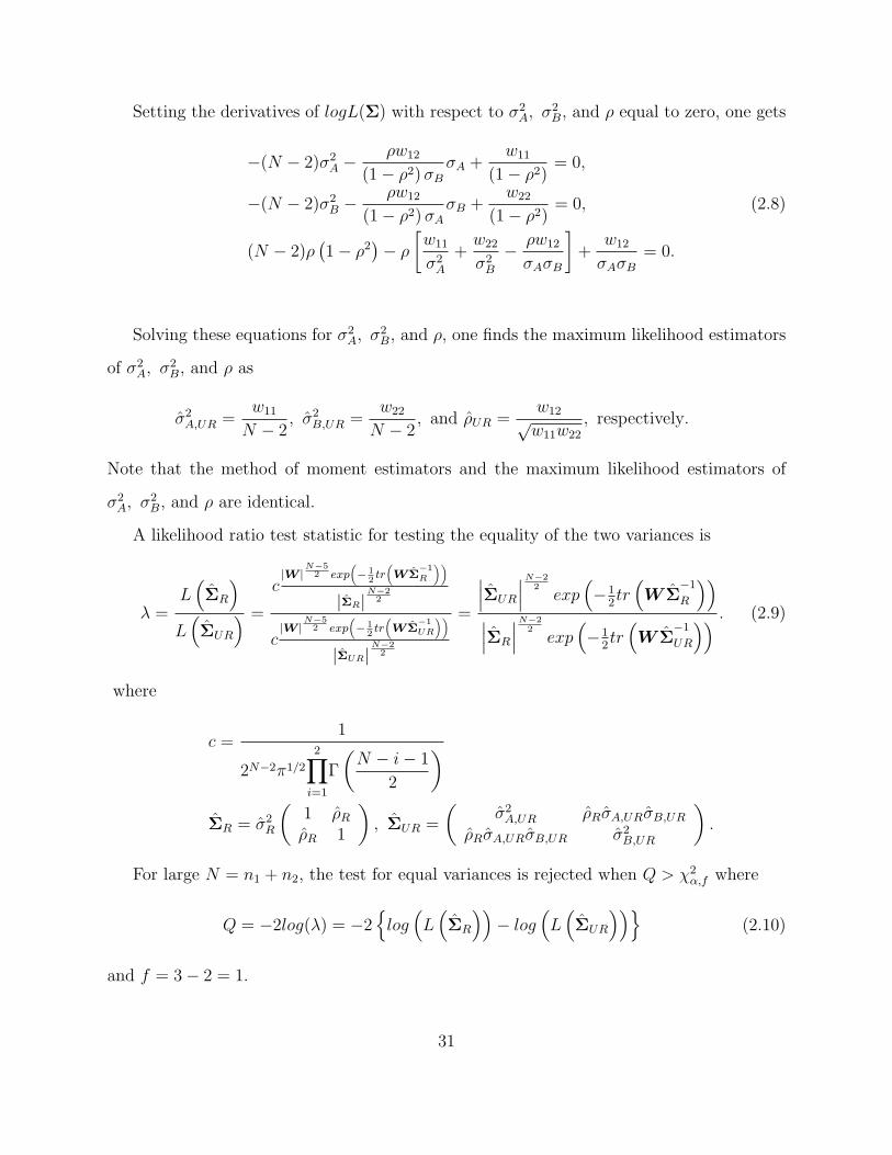
Setting the derivatives of logL(Σ) with respect to σ2A, σ
2B, and ρ equal to zero, one gets
−(N − 2)σ2A −
ρw12
(1− ρ2)σBσA +
w11
(1− ρ2)= 0,
−(N − 2)σ2B −
ρw12
(1− ρ2)σAσB +
w22
(1− ρ2)= 0, (2.8)
(N − 2)ρ(1− ρ2
)− ρ
[w11
σ2A
+w22
σ2B
− ρw12
σAσB
]+
w12
σAσB= 0.
Solving these equations for σ2A, σ
2B, and ρ, one finds the maximum likelihood estimators
of σ2A, σ
2B, and ρ as
σ2A,UR =
w11
N − 2, σ2
B,UR =w22
N − 2, and ρUR =
w12√w11w22
, respectively.
Note that the method of moment estimators and the maximum likelihood estimators of
σ2A, σ
2B, and ρ are identical.
A likelihood ratio test statistic for testing the equality of the two variances is
λ =L(ΣR
)L(ΣUR
) =
c|W |
N−52 exp
(− 1
2tr
(W Σ
−1R
))|ΣR|
N−22
c|W |
N−52 exp
(− 1
2tr
(W Σ
−1UR
))|ΣUR|
N−22
=
∣∣∣ΣUR
∣∣∣N−22exp
(−1
2tr(W Σ
−1
R
))∣∣∣ΣR
∣∣∣N−22exp
(−1
2tr(W Σ
−1
UR
)) . (2.9)
where
c =1
2N−2π1/2
2∏i=1
Γ
(N − i− 1
2
)ΣR = σ2
R
(1 ρRρR 1
), ΣUR =
(σ2A,UR ρRσA,URσB,UR
ρRσA,URσB,UR σ2B,UR
).
For large N = n1 + n2, the test for equal variances is rejected when Q > χ2α,f where
Q = −2log(λ) = −2{log(L(ΣR
))− log
(L(ΣUR
))}(2.10)
and f = 3− 2 = 1.
31
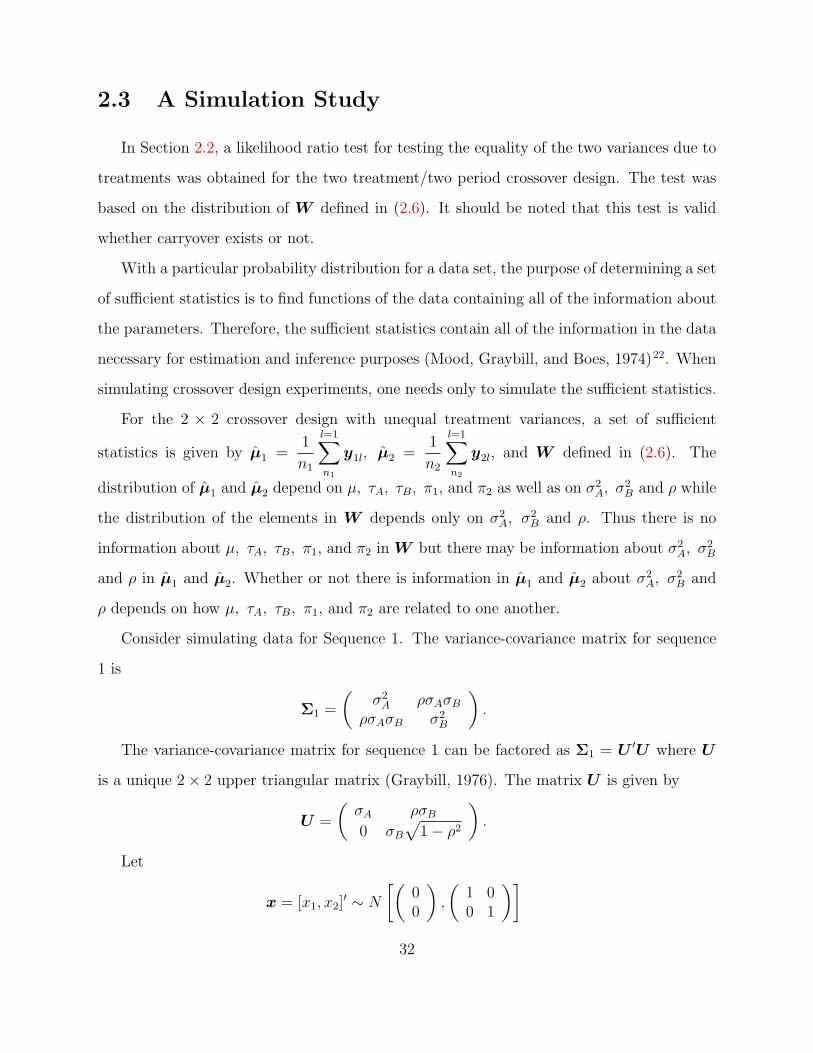
2.3 A Simulation Study
In Section 2.2, a likelihood ratio test for testing the equality of the two variances due to
treatments was obtained for the two treatment/two period crossover design. The test was
based on the distribution of W defined in (2.6). It should be noted that this test is valid
whether carryover exists or not.
With a particular probability distribution for a data set, the purpose of determining a set
of sufficient statistics is to find functions of the data containing all of the information about
the parameters. Therefore, the sufficient statistics contain all of the information in the data
necessary for estimation and inference purposes (Mood, Graybill, and Boes, 1974)22. When
simulating crossover design experiments, one needs only to simulate the sufficient statistics.
For the 2 × 2 crossover design with unequal treatment variances, a set of sufficient
statistics is given by µ1 =1
n1
l=1∑n1
y1l, µ2 =1
n2
l=1∑n2
y2l, and W defined in (2.6). The
distribution of µ1 and µ2 depend on µ, τA, τB, π1, and π2 as well as on σ2A, σ
2B and ρ while
the distribution of the elements in W depends only on σ2A, σ
2B and ρ. Thus there is no
information about µ, τA, τB, π1, and π2 in W but there may be information about σ2A, σ
2B
and ρ in µ1 and µ2. Whether or not there is information in µ1 and µ2 about σ2A, σ
2B and
ρ depends on how µ, τA, τB, π1, and π2 are related to one another.
Consider simulating data for Sequence 1. The variance-covariance matrix for sequence
1 is
Σ1 =
(σ2A ρσAσB
ρσAσB σ2B
).
The variance-covariance matrix for sequence 1 can be factored as Σ1 = U ′U where U
is a unique 2× 2 upper triangular matrix (Graybill, 1976). The matrix U is given by
U =
(σA ρσB0 σB
√1− ρ2
).
Let
x = [x1, x2]′ ∼ N
[(00
),
(1 00 1
)]32

and let
y = U ′x =
(σA 0
ρσB σB√
1− ρ2
)[x1
x2
].
Then
y ∼ N
[(00
),
(σ2A ρσAσB
ρσAσB σ2B
)].
The elements of y are y1 = σax1 and y2 = ρσBx1 + σB√
1− ρ2x2. For the simulations
performed, the x’s were generated from a standard normal distribution and the above trans-
formations were made to get the y’s. Furthermore, appropriate cell parameters were added
to the y’s to get the expected cell means. For example, appropriate cell parameters for se-
quence 1 yield y∗1 = y1 +µ+ τA+π1 for period 1 and y∗2 = y2 +µ+ τB +π2 +λA for period 2.
Without loss of generality, µ, π1, π2, τ1, τ2 and λA were all fixed at zero in the simulation
study. Data for sequence 2 were similarly generated using the variance-covariance matrix
Σ2 =
(σ2B ρσAσB
ρσAσB σ2A
).
and appropriate cell mean parameters.
Table 2.6 shows the parameters that were used when simulating data for Type I error
rate and power analysis for testing the equality of variances due to treatments.
Table 2.6: Parameter values used in Type I error rate and Power Analysis for the equality ofvariances due to Treatment in a Two Treatment/ Two Sequence Crossover Design (AB/BA)for Model (2.1)
λA = λB = 0, σ2A = 1
ρ Equal Variance Unequal Variance0 σ2
B = 1 σ2B = 2, 4, 8, 16
0.1 σ2B = 1 σ2
B = 2, 4, 8, 160.3 σ2
B = 1 σ2B = 2, 4, 8, 16
0.5 σ2B = 1 σ2
B = 2, 4, 8, 160.7 σ2
B = 1 σ2B = 2, 4, 8, 16
0.9 σ2B = 1 σ2
B = 2, 4, 8, 16
The number of subjects assigned to each sequence are n = 3, 6, 12, 18, 24 for each
of the cases described in Table 2.6. The empirical Type I error rates are estimated for the
33

equal variances case, and the power is estimated for each of the unequal variance cases. To
get the empirical Type I error rates and the power, 1000 simulations were done for each
n, ρ and σ2B.
To estimate parameters, the proposed method described in Section 2.2 is used in R. Using
the same data generated in R, restricted maximum likelihood ratio tests using SAS-MIXED
were also obtained. The SAS steps used are shown below. The programming statements
used in R are shown in Appendix E.
Step 1 Import data
INFILE ’C:\Data\KSU PhD THESIS\PRG\CS-2s2p2t-y6-18data.txt’ DELIMITER=’ ’;
INPUT rho sA2 sB2 nsubj sim seq subj y1 y2;
Step 2 Define period and arrange treatments
DATA one; SET one;
DROP y1 y2 ;
per=1; y=y1; output;
per=2; y=y2; output;
RUN;
DATA one; SET one;
SUbJ=subj+(seq-1)*nsubj;
trt=’A’;
IF seq=1 and per=2 THEN trt=’B’;
IF seq=2 and per=1 THEN trt=’B’;
RUN;
Step 3 Calculate −2log(L(ΣR
))in (2.10)
PROC MIXED ic data=one;
TITLE ’ANALYSIS USING SAS-MIXED’;
34

by rho sim;
CLASSES seq per trt subj;
MODEL y=seq trt per/DDFM=SATTERTH;
REPEATED trt/ SUBJECT=subj TYPE=CS;
ods listing exclude all;
ods output infocrit = null COVPARMS=HOPARMS;
RUN;
DATA null; set null;
rename neg2loglike =ho;
drop aic--caic;
Step 4 Calculate −2log(L(ΣUR
))in (2.10)
PROC MIXED ic data=one;
TITLE ’ANALYSIS USING SAS-MIXED’;
by rho sim;
CLASSES seq per trt subj;
MODEL y=seq trt per/DDFM=SATTERTH;
REPEATED trt/ SUBJECT=subj TYPE=CSH;
ods listing exclude all;
ods output infocrit = ha COVPARMS=HAPARMS;
RUN;
DATA ha; set ha;
rename neg2loglike =ha;
drop aic--caic;
Step 5 Calculate the Type I error rate
DATA comb; SET comb;
35
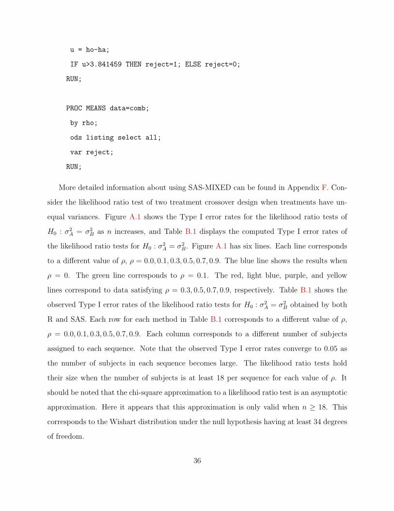
u = ho-ha;
IF u>3.841459 THEN reject=1; ELSE reject=0;
RUN;
PROC MEANS data=comb;
by rho;
ods listing select all;
var reject;
RUN;
More detailed information about using SAS-MIXED can be found in Appendix F. Con-
sider the likelihood ratio test of two treatment crossover design when treatments have un-
equal variances. Figure A.1 shows the Type I error rates for the likelihood ratio tests of
H0 : σ2A = σ2
B as n increases, and Table B.1 displays the computed Type I error rates of
the likelihood ratio tests for H0 : σ2A = σ2
B. Figure A.1 has six lines. Each line corresponds
to a different value of ρ, ρ = 0.0, 0.1, 0.3, 0.5, 0.7, 0.9. The blue line shows the results when
ρ = 0. The green line corresponds to ρ = 0.1. The red, light blue, purple, and yellow
lines correspond to data satisfying ρ = 0.3, 0.5, 0.7, 0.9, respectively. Table B.1 shows the
observed Type I error rates of the likelihood ratio tests for H0 : σ2A = σ2
B obtained by both
R and SAS. Each row for each method in Table B.1 corresponds to a different value of ρ,
ρ = 0.0, 0.1, 0.3, 0.5, 0.7, 0.9. Each column corresponds to a different number of subjects
assigned to each sequence. Note that the observed Type I error rates converge to 0.05 as
the number of subjects in each sequence becomes large. The likelihood ratio tests hold
their size when the number of subjects is at least 18 per sequence for each value of ρ. It
should be noted that the chi-square approximation to a likelihood ratio test is an asymptotic
approximation. Here it appears that this approximation is only valid when n ≥ 18. This
corresponds to the Wishart distribution under the null hypothesis having at least 34 degrees
of freedom.
36

Next consider data that were generated when σ2A 6= σ2
B. Figure A.2 shows the power of
the LRT of σ2A = σ2
B when (σ2A, σ
2B) = (1, 2) for each value of ρ. As the number of subjects
is increased from 6 to 24, the power increases sharply towards 1 when ρ = 0.9. And, as the
value of the correlation, ρ, increases from 0.1 to 0.9, the power also increases. Table B.2
shows the observed power for different variances, (σ2A, σ
2B) = (1, 2). The performance of the
two tests for the equality of variances given by R and SAS are identical. Figures A.3-A.5
show the trend for other values of σ2B. When the value of σ2
B increases to 4, 8, and 16,
the power is very close to 1 for most configurations of the other parameters. And, as the
value of correlation, ρ, is increased from 0.1 to 0.9, the power is close to 1. Tables B.3-B.5
display the observed power for as the σ2B increases. The performance to test the equality
of two variances by R and SAS are identical. Note that the power value for small numbers
of subjects per sequence may be misleading since the desired Type I error rates are not
achieved when n ≤ 12.
37

2.4 Two Treatment/ Two sequence Crossover Design
Balanced for Carryover Effect
When carryover effects exist, they are aliased with period and treatment effects in the
2×2 crossover design. Carryover effects are also aliased with sequence effects. Two treatment
crossover designs that are balanced for carryover effects can be used to separate treatment,
period and sequence effects from carryover effects. These two treatment crossover designs
that can be used to estimate treatment differences free from carryover effects include extra
sequence(s) and/or period(s) as described in Section 1.2.
2.4.1 Two Treatment/ Two Sequence Dual Balanced Design
Consider the ABA/BAB dual balanced design. The ABA/BAB crossover design is given
in Table 2.7.
Table 2.7: A Two Treatment/ Two Sequence Crossover Design with an Extra Period(ABA/BAB)
PeriodSequence 1 2 3
1 A B A2 B A B
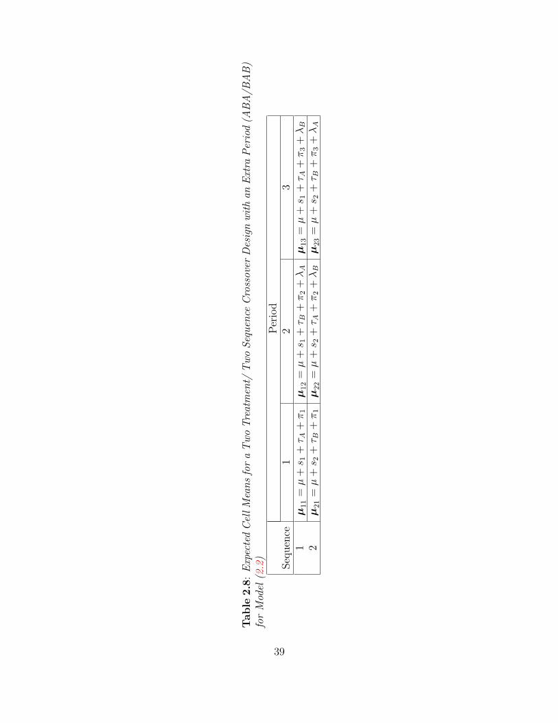
The expected cell means for the ABA/BAB crossover design in Table 2.7 are given in
Table 2.8.
38
Table
2.8
:E
xpec
ted
Cel
lM
ean
sfo
ra
Tw
oT
reat
men
t/T
wo
Seq
uen
ceC
ross
over
Des
ign
wit
han
Ext
raP
erio
d(A
BA
/BA
B)
for
Mod
el(2
.2)
Per
iod
Seq
uen
ce1
23
1µ
11
=µ
+s 1
+τ A
+π
1µ
12
=µ
+s 1
+τ B
+π
2+λA
µ13
=µ
+s 1
+τ A
+π
3+λB
2µ
21
=µ
+s 2
+τ B
+π
1µ
22
=µ
+s 2
+τ A
+π
2+λB
µ23
=µ
+s 2
+τ B
+π
3+λA
39

Define the sums of squares for the two sequences by
W1 =
n1∑l=1
(yy1l − µ1) (yy1l − µ1)T
=
n1∑l=1
y111l − y111.
y122l − y122.
y113l − y113.
y111l − y111.
y122l − y122.
y113l − y113.
T
=
w111 w112 w113
w112 w122 w123
w113 w123 w133
and
W2 =
n2∑l=1
(yy2l − µ2) (yy2l − µ2)T
=
n2∑l=1
y221l − y221.
y212l − y212.
y223l − y223.
y221l − y221.
y212l − y212.
y223l − y223.
T
=
w211 w212 w213
w212 w222 w223
w213 w223 w233
.
Then Wi, i = 1, 2 has a Wishart distribution with ni−1 degrees of freedom and variance-
covariance structure Σi, i = 1, 2. Assuming compound symmetry for time period correla-
tions together with unequal variances for the treatments, the variance-covariance matrices
for the two sequences are given as
Σ1 =
σ2A ρσAσB ρσ2
A
ρσAσB σ2B ρσAσB
ρσ2A ρσAσB σ2
A
= D1/21 RD
1/21
and
Σ2 =
σ2B ρσAσB ρσ2
B
ρσAσB σ2A ρσAσB
ρσ2B ρσAσB σ2
B
= D1/22 RD
1/22 .
where
D1/21 = diag(σA, σB, σA), D
1/22 = diag(σB, σA, σB), and R =
1 ρ ρρ 1 ρρ ρ 1
.Note that
D−1/21 = diag
(1
σA,
1
σB,
1
σA
), D
−1/22 = diag
(1
σB,
1
σA,
1
σB
),
and
R−1 =1
(1− ρ)(1 + 2ρ)
1 + ρ −ρ −ρ−ρ 1 + ρ −ρ−ρ −ρ 1 + ρ
.40
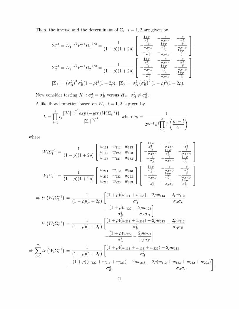
Then, the inverse and the determinant of Σi, i = 1, 2 are given by
Σ−11 = D
−1/21 R−1D
−1/21 =
1
(1− ρ)(1 + 2ρ)
1+ρσ2A
− ρσAσB
− ρσ2A
− ρσAσB
1+ρσ2B
− ρσAσB
− ρσ2A− ρσAσB
1+ρσ2A
,
Σ−12 = D
−1/22 R−1D
−1/22 =
1
(1− ρ)(1 + 2ρ)
1+ρσ2B
− ρσAσB
− ρσ2B
− ρσAσB
1+ρσ2A
− ρσAσB
− ρσ2B− ρσAσB
1+ρσ2B
,|Σ1| =
(σ2A
)2σ2B(1− ρ)2(1 + 2ρ), |Σ2| = σ2
A
(σ2B
)2(1− ρ)2(1 + 2ρ).
Now consider testing H0 : σ2A = σ2
B versus HA : σ2A 6= σ2
B.
A likelihood function based on Wi, i = 1, 2 is given by
L =2∏i=1
ci|Wi|
ni−5
2 exp(−1
2tr(WiΣ
−1i
))|Σi|
ni−1
2
where ci =1
2ni−1π3
3∏l=1
Γ
(ni − l
2
)where
W1Σ−11 =
1
(1− ρ)(1 + 2ρ)
w111 w112 w113
w112 w122 w123
w113 w123 w133
1+ρσ2A
− ρσAσB
− ρσ2A
− ρσAσB
1+ρσ2B
− ρσAσB
− ρσ2A− ρσAσB
1+ρσ2A
W2Σ−12 =
1
(1− ρ)(1 + 2ρ)
w211 w212 w213
w212 w222 w223
w213 w223 w233
1+ρσ2B
− ρσAσB
− ρσ2B
− ρσAσB
1+ρσ2A
− ρσAσB
− ρσ2B− ρσAσB
1+ρσ2B
⇒ tr(W1Σ
−11
)=
1
(1− ρ)(1 + 2ρ)
[(1 + ρ)(w111 + w133)− 2ρw113
σ2A
− 2ρw112
σAσB
+(1 + ρ)w122
σ2B
− 2ρw123
σAσB
]tr(W2Σ
−12
)=
1
(1− ρ)(1 + 2ρ)
[(1 + ρ)(w211 + w233)− 2ρw213
σ2B
− 2ρw212
σAσB
+(1 + ρ)w222
σ2A
− 2ρw223
σAσB
]⇒
2∑i=1
tr(WiΣ
−1i
)=
1
(1− ρ)(1 + 2ρ)
[(1 + ρ)(w111 + w133 + w222)− 2ρw113
σ2A
+(1 + ρ)(w122 + w211 + w233)− 2ρw213
σ2B
− 2ρ(w112 + w123 + w212 + w223)
σAσB
].
41

The log-likelihood function is
logL =2∑i=1
[log(ci) +
ni − 5
2log|Wi| −
ni − 1
2log|Σi| −
1
2tr(WiΣ
−1i
)].
Under H0 : σ2A = σ2
B = σ2,
|Σ1| = |Σ2| = (1− ρ)2(1 + 2ρ)σ6,
tr(W1Σ
−11
)=
1
(1− ρ)(1 + 2ρ)σ2{(1 + ρ)(w111 + w122 + w133)− 2ρ(w112 + w113 + w123)} ,
tr(W2Σ
−12
)=
1
(1− ρ)(1 + 2ρ)σ2{(1 + ρ)(w211 + w222 + w233)− 2ρ(w212 + w213 + w223)} .
Therefore, the log-likelihood function is
logL =2∑i=1
log(ci) +2∑i=1
ni − 5
2log|Wi| −
N − 2
2log[(1− ρ)2(1 + 2ρ)
]−3(N − 2)
2log(σ2)− 1
2(1− ρ)(1 + 2ρ)σ2[(1 + ρ)A− 2ρB] .
where
A = w111 + w122 + w133 + w211 + w222 + w233
B = w112 + w113 + w123 + w212 + w213 + w223, and N =2∑i=1
ni.
The derivatives of logL with respect to σ2 and ρ are
∂logL
∂σ2= −3(N − 2)
2σ2+
1
2(1− ρ)(1 + 2ρ)σ4[(1 + ρ)A− 2ρB] ,
∂logL
∂ρ=
3(N − 2)ρ(1− ρ)
(1− ρ)2(1 + 2ρ)− 2 [ρ(2 + ρ)A− (1 + 2ρ2)B]
2(1− ρ)2(1 + 2ρ)2σ2.
Setting the derivatives of logL with respect to σ2 and ρ equal to zero, one gets
−3(N − 2)σ2 +(1 + ρ)A− 2ρB
(1− ρ)(1 + 2ρ)= 0,
3(N − 2)ρ(1− ρ)(1 + 2ρ)− ρ(2 + ρ)A− (1 + 2ρ2)B
σ2= 0.
Then, under H0 : σ2A = σ2
B = σ2, the maximum likelihood estimator of σ2 and ρ is
σ2R =
A
3(N − 2)and ρR =
B
A, respectively.
42

where
A = w111 + w122 + w133 + w211 + w222 + w233
B = w112 + w113 + w123 + w212 + w213 + w223.
Under HA : σ2A 6= σ2
B,
|Σ1| =(σ2A
)2σ2B(1− ρ)2(1 + 2ρ), |Σ2| = σ2
A
(σ2B
)2(1− ρ)2(1 + 2ρ),
tr(W1Σ
−11
)=
1
(1− ρ)(1 + 2ρ)
[(1 + ρ)(w111 + w133)− 2ρw113
σ2A
− 2ρw112
σAσB
+(1 + ρ)w122
σ2B
− 2ρw123
σAσB
],
tr(W2Σ
−12
)=
1
(1− ρ)(1 + 2ρ)
[(1 + ρ)(w211 + w233)− 2ρw213
σ2B
− 2ρw212
σAσB
+(1 + ρ)w222
σ2A
− 2ρw223
σAσB
].
Therefore the log-likelihood function is
logL =2∑i=1
log(ci) +2∑i=1
ni − 5
2log|Wi| −
2n1 + n2 − 3
2log(σ2A
)−n1 + 2n2 − 3
2log(σ2B
)− N − 2
2log[(1− ρ)2(1 + 2ρ)
]− 1
2(1− ρ)(1 + 2ρ)
[(1 + ρ)(w111 + w133 + w222)− 2ρw113
σ2A
+(1 + ρ)(w122 + w211 + w233)− 2ρw213
σ2B
− 2ρ(w112 + w123 + w212 + w223)
σAσB
].
The derivatives of logL with respect to σ2A, σ
2B, and ρ are
∂logL
∂σ2A
= −2n1 + n2 − 3
2σ2A
+(1 + ρ)(w111 + w133 + w222)− 2ρw113
2(1− ρ)(1 + 2ρ) (σ2A)
2
−2ρ(w112 + w123 + w212 + w223)
4(1− ρ)(1 + 2ρ) (σA)3 σB,
∂logL
∂σ2B
= −n1 + 2n2 − 3
2σ2B
+(1 + ρ)(w122 + w211 + w233)− 2ρw213
2(1− ρ)(1 + 2ρ) (σ2B)
2 (2.11)
−2ρ(w112 + w123 + w212 + w223)
4(1− ρ)(1 + 2ρ)σA (σB)3 ,
43

∂logL
∂ρ=
3(N − 2)ρ(1− ρ)
(1− ρ)2(1 + 2ρ)− 1
2(1− ρ)2(1 + 2ρ)2×{
2ρ(2 + ρ)(w111 + w133 + w222)
σ2A
+2ρ(2 + ρ)(w122 + w211 + w233)
σ2B
−2(1 + 2ρ2)
[w113
σ2A
+w213
σ2B
+(w112 + w123 + w212 + w223)
σAσB
]}.
Setting the derivatives of logL with respect to σ2A, σ
2B, and ρ equal to zero, one gets
(2n1 + n2 − 3)σ2A +
ρ(w112 + w123 + w212 + w223)(1− ρ)(1 + 2ρ)σB
σA −(1 + ρ)(w111 + w133 + w222)− 2ρw113
(1− ρ)(1 + 2ρ)= 0,
(n1 + 2n2 − 3)σ2B +
ρ(w112 + w123 + w212 + w223)(1− ρ)(1 + 2ρ)σA
σB −(1 + ρ)(w122 + w211 + w233)− 2ρw213
(1− ρ)(1 + 2ρ)= 0,
6(N − 2)ρ(1− ρ)(1 + 2ρ)−{
2ρ(2 + ρ)(w111 + w133 + w222)σ2A
+2ρ(2 + ρ)(w122 + w211 + w233)
σ2B
−2(1 + 2ρ2)[w113
σ2A
+w213
σ2B
+(w112 + w123 + w212 + w223)
σAσB
]}. (2.12)
Unfortunately, the maximum likelihood estimators of σ2A, σ
2B and ρ do not have a closed
form solution. An iterative process to find solutions for σ2A,UR, σ
2B,UR and ρUR is discussed in
Section 2.4.2. Shanga (2003)28 incorrectly claimed that the maximum likelihood estimators
of σ2A, σ
2B and ρ were
σ2A,UR =
w11
2n1 + n2 − 3, σ2
B,UR =w22
n1 + 2n2 − 3, ρUR =
1
3
[w12√w11w22
+w∗11
w11
+w∗22
w22
]. (2.13)
where w11 = w111 + w133 + w222, w22 = w122 + w211 + w233, w12 = w112 + w123 + w212 + w223,
w∗11 = w113, and w∗22 = w213.
The likelihood ratio test statistic for testing the equality of the two variances is
λ =LRLUR
=
2∏i=1
ci|Wi|
ni−5
2 exp(−1
2tr(WiΣ
−1i,R
))|Σi,R|
ni−1
2
2∏i=1
ci|Wi|
ni−5
2 exp(−1
2tr(WiΣ
−1i,UR
))|Σi,UR|
ni−1
2
=
2∏i=1
|Σi,UR|ni−1
2
2∏i=1
exp
(−1
2tr(WiΣ
−1i,R
))2∏i=1
|Σi,R|ni−1
2
2∏i=1
exp
(−1
2tr(WiΣ
−1i,UR
)) .
44
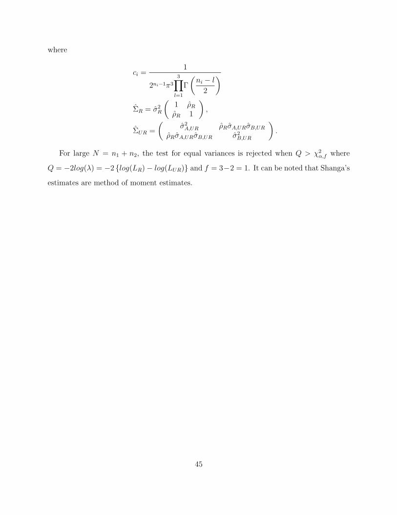
where
ci =1
2ni−1π3
3∏l=1
Γ
(ni − l
2
)ΣR = σ2
R
(1 ρRρR 1
),
ΣUR =
(σ2A,UR ρRσA,URσB,UR
ρRσA,URσB,UR σ2B,UR
).
For large N = n1 + n2, the test for equal variances is rejected when Q > χ2α,f where
Q = −2log(λ) = −2 {log(LR)− log(LUR)} and f = 3−2 = 1. It can be noted that Shanga’s
estimates are method of moment estimates.
45
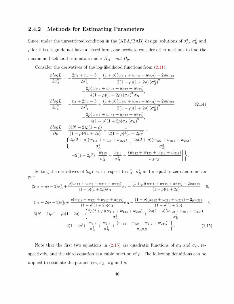
2.4.2 Methods for Estimating Parameters
Since, under the unrestricted condition in the (ABA/BAB) design, solutions of σ2A, σ
2B and
ρ for this design do not have a closed form, one needs to consider other methods to find the
maximum likelihood estimators under HA : not H0.
Consider the derivatives of the log-likelihood functions from (2.11):
∂logL
∂σ2A
= −2n1 + n2 − 3
2σ2A
+(1 + ρ)(w111 + w133 + w222)− 2ρw113
2(1− ρ)(1 + 2ρ) (σ2A)
2
−2ρ(w112 + w123 + w212 + w223)
4(1− ρ)(1 + 2ρ) (σA)3 σB,
∂logL
∂σ2B
= −n1 + 2n2 − 3
2σ2B
+(1 + ρ)(w122 + w211 + w233)− 2ρw213
2(1− ρ)(1 + 2ρ) (σ2B)
2 (2.14)
−2ρ(w112 + w123 + w212 + w223)
4(1− ρ)(1 + 2ρ)σA (σB)3 ,
∂logL
∂ρ=
3(N − 2)ρ(1− ρ)
(1− ρ)2(1 + 2ρ)− 1
2(1− ρ)2(1 + 2ρ)2×{
2ρ(2 + ρ)(w111 + w133 + w222)
σ2A
+2ρ(2 + ρ)(w122 + w211 + w233)
σ2B
−2(1 + 2ρ2)
[w113
σ2A
+w213
σ2B
+(w112 + w123 + w212 + w223)
σAσB
]}.
Setting the derivatives of logL with respect to σ2A, σ
2B and ρ equal to zero and one can
get:
(2n1 + n2 − 3)σ2A +
ρ(w112 + w123 + w212 + w223)(1− ρ)(1 + 2ρ)σB
σA −(1 + ρ)(w111 + w133 + w222)− 2ρw113
(1− ρ)(1 + 2ρ)= 0,
(n1 + 2n2 − 3)σ2B +
ρ(w112 + w123 + w212 + w223)(1− ρ)(1 + 2ρ)σA
σB −(1 + ρ)(w122 + w211 + w233)− 2ρw213
(1− ρ)(1 + 2ρ)= 0,
6(N − 2)ρ(1− ρ)(1 + 2ρ)−{
2ρ(2 + ρ)(w111 + w133 + w222)σ2A
+2ρ(2 + ρ)(w122 + w211 + w233)
σ2B
−2(1 + 2ρ2)[w113
σ2A
+w213
σ2B
+(w112 + w123 + w212 + w223)
σAσB
]}. (2.15)
Note that the first two equations in (2.15) are quadratic functions of σA and σB, re-
spectively, and the third equation is a cubic function of ρ. The following definitions can be
applied to estimate the parameters, σA, σB and ρ.
46

Definition 2. (Quadratic Equations) Solutions of any quadratic equation, ax2 + bx+ c = 0,
are given by
x =−b±
√b2 − 4ac
2a.
If a, b, and c are real, the solutions are as follows:
• If b2 − 4ac is positive, the roots are real and unequal.
• If b2 − 4ac is zero, the roots are real and equal.
• If b2 − 4ac is negative, the roots are imaginary and unequal.
Definition 3. (Cubic Equations) When one has a cubic equation, y3 + py2 + qy + r = 0,
it can be transformed to x3 + ax + b = 0 by substituting x− p3
for y, where a = 12
(3q − p2)
and b = 127
(2p3 − 9pq + 27r). Let A = 3
√− b
2+√
b2
4+ a3
27and B = 3
√− b
2−√
b2
4+ a3
27, then
x = A+B, −A+B2
+ A−B2
√−3, and −A+B
2− A−B
2
√−3 are solutions.
If p, q, r are real, then
• If b2
4+ a3
27> 0, there will be one real root and two conjugate imaginary roots.
• If b2
4+ a3
27= 0, there will be three real roots of which at least two are equal.
• If b2
4+ a3
27< 0, there will be three real and unequal roots.
The following iterative procedure can be used to find the maximum likelihood estimates
of σA, σB and ρ under HA.
Procedure
1. Set starting values using the method of moment estimates from (2.13):
σ0A =
√σ2A,UR, σ
0B =
√σ2B,UR, and ρ0 = ρUR
47

σ2A,UR =
w11
2n1 + n2 − 3, σ2
B,UR =w22
n1 + 2n2 − 3, and ρUR =
1
3
[w12√w11w22
+w∗11
w11
+w∗22
w22
].
where w11 = w111 +w133 +w222, w22 = w122 +w211 +w233, w∗11 = w113, and w∗22 = w213.
2. Plug σ0B, and ρ0 into the quadratic equation of σA:
(2n1 + n2 − 3)σ2A +
ρ0(w112 + w123 + w212 + w223)
(1− ρ0)(1 + 2ρ0)σ0B
σA
− (1 + ρ0)(w111 + w133 + w222)− 2ρ0w113
(1− ρ0)(1 + 2ρ0)= 0.
And obtain a solution for the parameter, σA by using Definition 2: call the solution,
σA.
3. Plug σA, and ρ0 into the quadratic equation of σB:
(n1 + 2n2 − 3)σ2B +
ρ0(w112 + w123 + w212 + w223)
(1− ρ0)(1 + 2ρ0)σAσB
− (1 + ρ0)(w122 + w211 + w233)− 2ρ0w213
(1− ρ0)(1 + 2ρ0)= 0.
And obtain a solution for the parameter, σB by using Definition 2: call the solution,
σB.
4. Plug σA, and σB into the cubic equation of ρ:
6(N − 2)ρ(1− ρ)(1 + 2ρ)−{
2ρ(2 + ρ)(w111 + w133 + w222)− (1 + 2ρ2)(w113 + w131)
σ2A
+2ρ(2 + ρ)(w122 + w211 + w233)− (1 + 2ρ2)(w213 + w231)
σ2B
−2(w112 + w123 + w212 + w223)(1 + 2ρ2)(1 + 2ρ2)
σAσB
}= 0.
And obtain a solution for the parameter, ρ, by using Definition 3: call the solution, ρ.
5. If |σA − σ0A| < ε, |σB − σ0
B| < ε, and |ρ− ρ0| < ε where ε = 10−5, then STOP and
use σA, σB, and ρ as maximum likelihood estimates of σA, σB, and ρ.
If |σA − σ0A| > ε or |σB − σ0
B| > ε or |ρ− ρ0| > ε, repeat steps 2-4 with σ0A ←
σA, σ0B ← σB, and ρ0 ← ρ.
No Simulations were carried out for the ABA/BAB design.
48

2.5 Conclusions
Data were generated for the likelihood ratio test of equal variances for both the null and
alternative cases. The Type I error rates for the likelihood ratio test of equal variance is
shown in Figure A.1 and Table B.1. The power results for the likelihood ratio tests are
shown in Figures A.2-A.5, and Tables B.2-B.5.
Figure A.1 and Table B.1 show that the LRT holds its size when the number of subjects
is greater than 18 per sequence. For the case of unequal variance, the power is sharply
increased close towards 1 as the number of subjects is increased and the value of variance
B is large when compared to the variance of A.
As a special case of two treatment crossover design balanced for carryover effects, ABA/BAB
dual balanced design is introduced. Under H0 : σ2A = σ2
B = σ2, the maximum likelihood esti-
mator of σ2 and ρ has closed form solution, respectively. However, under H0 : σ2A 6= σ2
B, the
maximum likelihood estimators of σ2A, σ
2B and ρ do not have closed form solutions. There-
fore, a procedure to estimate parameters is introduced in Section 2.4.2. This procedure will
be applied in Chapter 3 for a three treatment crossover design, and the performance will be
assessed by examining the Type I error rates and power.
49

2.6 Future Work
In this chapter, two treatment crossover designs with data that have unequal variances are
considered. In particular, two kinds of crossover designs were considered; one is a crossover
design having the number of treatments equal to the number of periods (t = p = 2), AB/BA,
and the other is a crossover design balanced for carryover effects known as dual balanced
design, ABA/BAB, which is different between the number of treatment and the number of
period.
Future work will also consider testing the equality of the variances due to treatments
with crossover designs balanced for carryover effects such as the extra period designs, the
ABB/BAA and ABA/ABB/BAB/BAA, and/or designs with extra sequence(s) such as
Balaam design, AB/BA/AA/BB.
50
Chapter 3
Testing for Equal TreatmentVariances in a Three TreatmentCrossover Design
3.1 Introduction
A crossover design is an experimental design in which each experimental unit receives a
series of experimental treatments over time. The order that an experimental unit receives
its treatments is called a sequence (for example, the sequence ABC means that treatment
A is given first, and then followed by treatment B, then followed by treatment C). A period
is the time interval during which a treatment is administered to the experimental unit. A
period could range from a few minutes to several months depending on the study. Sequences
usually involve subjects receiving a different treatment in each successive period. However,
treatments may occur more than once in any sequence (example, ABAB).
The basic three treatment crossover design is a cyclic crossover design denoted by
ABC/BCA/CAB. It means that treatment B always follows treatment A, treatment C
always follows treatment B, and treatment A always follows treatment C. In the three
treatment/ three sequence crossover design, ABC is the order of the treatments A, B and
C in the first sequence, BCA is the order of the treatments B, C and A in the second
sequence and CAB is the order of the treatments C, A and B in the third sequence. The
three treatment/ three sequence crossover design will be referred to as 3×3 crossover design.
51

The cyclic crossover design, ABC/BCA/CAB, is not balanced for carryover effects.
In the three treatment design, a Williams’ design is recommended. Williams (1949)30
developed a procedure using Latin square designs that balance crossover designs for carryover
effects when the number of periods is equal to the number of treatments (p = t > 2). The
Williams’ designs have the characteristic that every treatment follows every other treatment
an equal number of times. When implementing the Williams’ design procedure, two Latin
squares are generated for all experiments involving three or more treatments. Designs that
have an odd number of treatments require both the Latin squares to achieve balance for
carryover effects, and designs that have an even number of treatments require only one Latin
square. If the number of treatments is odd, each treatment follows every other treatment
twice. If the number of treatment is even, each treatment follow every other treatment
once. Mathews gives a clear description of a general algorithm for developing the Williams’
designs. The same description is also given by Jones and Kenward (2003)16.
Two Latin squares, six different sequences, are used to construct sequences such that
each treatment immediately follows every other treatment exactly twice. The three treat-
ment crossover design that is balanced for first order carryover effects has six sequences,
ABC/ACB/BAC/BCA/CAB/CBA. The six sequence crossover design is recommended
since the cyclic three treatment/ three sequence crossover design has carryover effects aliased
with treatment effects when carryover is present in the model.
Crossover designs are traditionally analyzed as split-plot designs. A split-plot design is
a design that has whole plot and subplot experimental units. The whole plot in a crossover
design is the subject to which a sequence of treatments has been assigned and the subplot is
the period. There are both between-subject comparisons and within-subject comparisons.
One would like treatment comparisons to be within-subject comparisons as within subject
variability is usually much smaller than between subject variability. The smaller within
subject variability allows for more precise estimators of treatment differences. The within
subject comparisons give the crossover design an advantage over a completely randomized
52
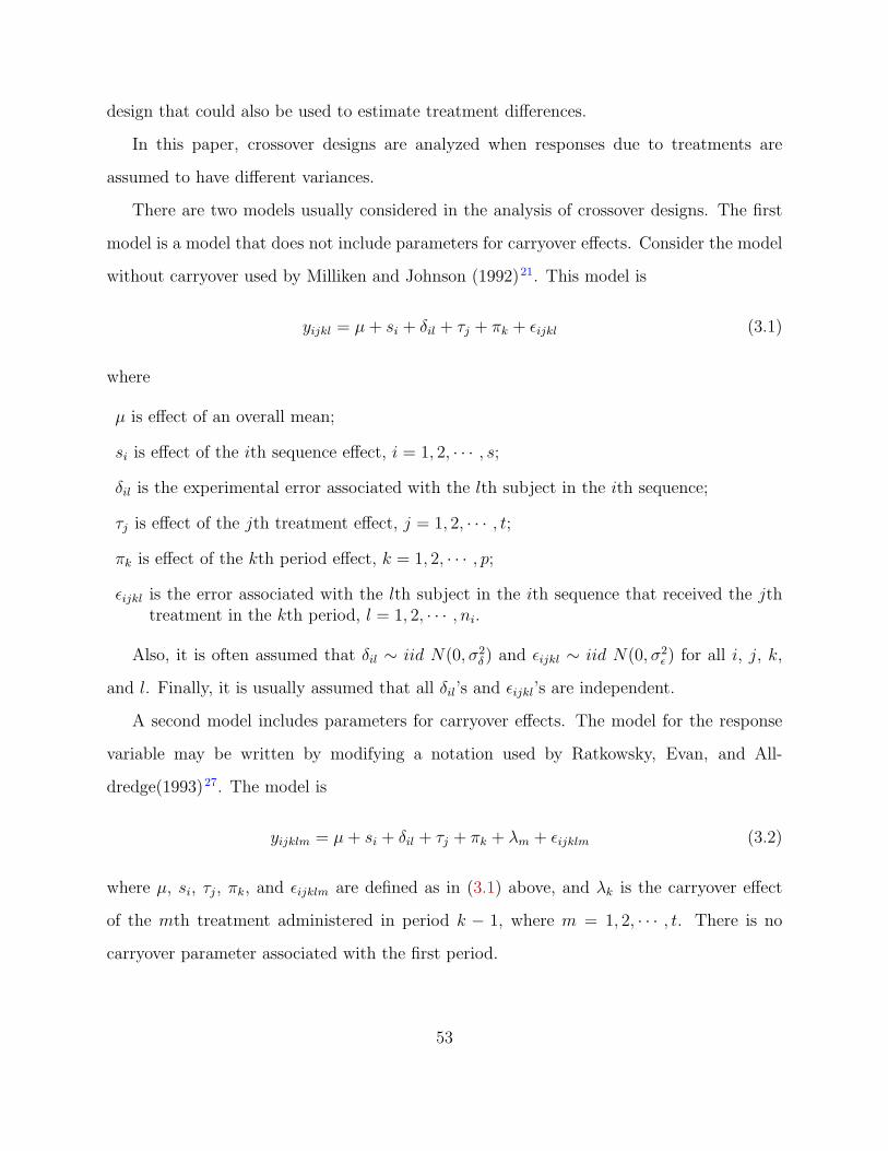
design that could also be used to estimate treatment differences.
In this paper, crossover designs are analyzed when responses due to treatments are
assumed to have different variances.
There are two models usually considered in the analysis of crossover designs. The first
model is a model that does not include parameters for carryover effects. Consider the model
without carryover used by Milliken and Johnson (1992)21. This model is
yijkl = µ+ si + δil + τj + πk + εijkl (3.1)
where
µ is effect of an overall mean;
si is effect of the ith sequence effect, i = 1, 2, · · · , s;
δil is the experimental error associated with the lth subject in the ith sequence;
τj is effect of the jth treatment effect, j = 1, 2, · · · , t;
πk is effect of the kth period effect, k = 1, 2, · · · , p;
εijkl is the error associated with the lth subject in the ith sequence that received the jthtreatment in the kth period, l = 1, 2, · · · , ni.
Also, it is often assumed that δil ∼ iid N(0, σ2δ ) and εijkl ∼ iid N(0, σ2
ε ) for all i, j, k,
and l. Finally, it is usually assumed that all δil’s and εijkl’s are independent.
A second model includes parameters for carryover effects. The model for the response
variable may be written by modifying a notation used by Ratkowsky, Evan, and All-
dredge(1993)27. The model is
yijklm = µ+ si + δil + τj + πk + λm + εijklm (3.2)
where µ, si, τj, πk, and εijklm are defined as in (3.1) above, and λk is the carryover effect
of the mth treatment administered in period k − 1, where m = 1, 2, · · · , t. There is no
carryover parameter associated with the first period.
53
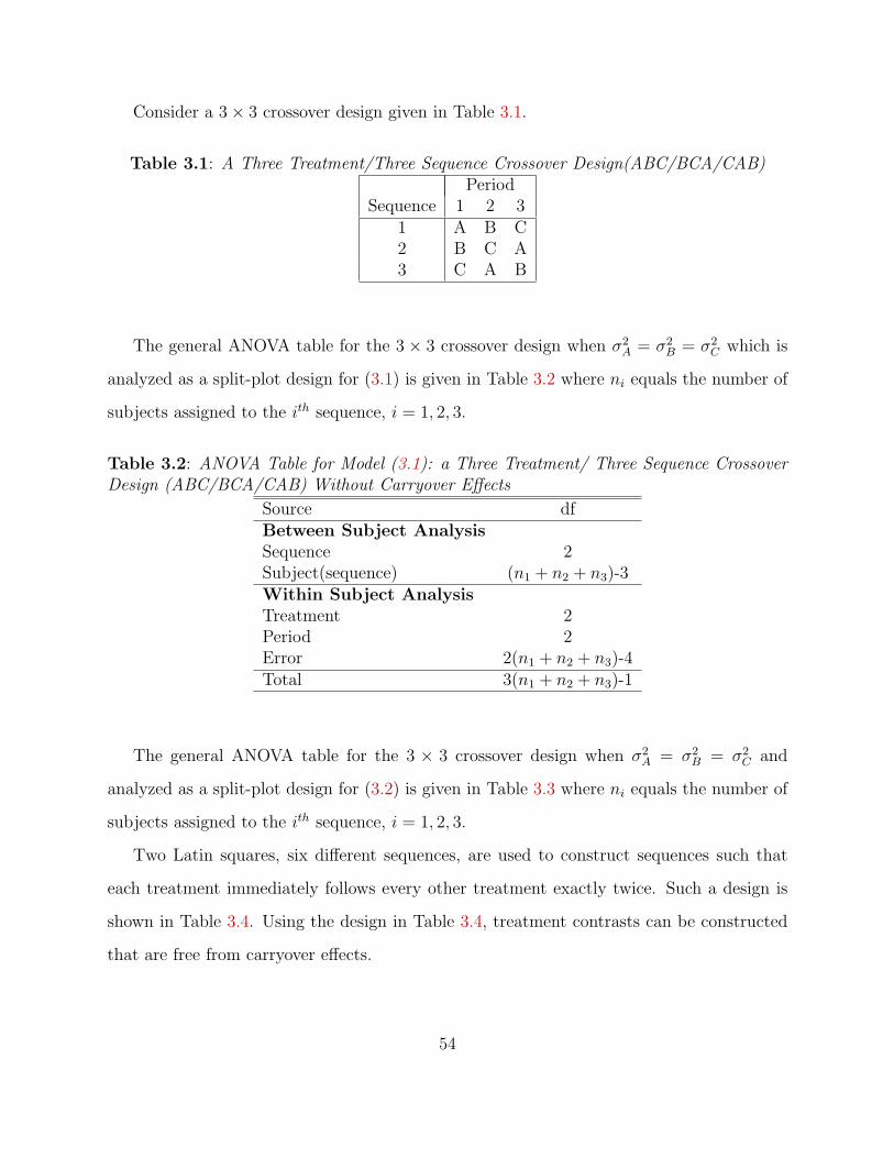
Consider a 3× 3 crossover design given in Table 3.1.
Table 3.1: A Three Treatment/Three Sequence Crossover Design(ABC/BCA/CAB)Period
Sequence 1 2 31 A B C2 B C A3 C A B
The general ANOVA table for the 3 × 3 crossover design when σ2A = σ2
B = σ2C which is
analyzed as a split-plot design for (3.1) is given in Table 3.2 where ni equals the number of
subjects assigned to the ith sequence, i = 1, 2, 3.
Table 3.2: ANOVA Table for Model (3.1): a Three Treatment/ Three Sequence CrossoverDesign (ABC/BCA/CAB) Without Carryover Effects
Source dfBetween Subject AnalysisSequence 2Subject(sequence) (n1 + n2 + n3)-3Within Subject AnalysisTreatment 2Period 2Error 2(n1 + n2 + n3)-4Total 3(n1 + n2 + n3)-1
The general ANOVA table for the 3 × 3 crossover design when σ2A = σ2
B = σ2C and
analyzed as a split-plot design for (3.2) is given in Table 3.3 where ni equals the number of
subjects assigned to the ith sequence, i = 1, 2, 3.
Two Latin squares, six different sequences, are used to construct sequences such that
each treatment immediately follows every other treatment exactly twice. Such a design is
shown in Table 3.4. Using the design in Table 3.4, treatment contrasts can be constructed
that are free from carryover effects.
54
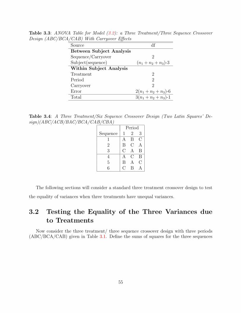
Table 3.3: ANOVA Table for Model (3.2): a Three Treatment/Three Sequence CrossoverDesign (ABC/BCA/CAB) With Carryover Effects
Source dfBetween Subject AnalysisSequence/Carryover 2Subject(sequence) (n1 + n2 + n3)-3Within Subject AnalysisTreatment 2Period 2Carryover 2Error 2(n1 + n2 + n3)-6Total 3(n1 + n2 + n3)-1
Table 3.4: A Three Treatment/Six Sequence Crossover Design (Two Latin Squares’ De-sign)(ABC/ACB/BAC/BCA/CAB/CBA)
PeriodSequence 1 2 3
1 A B C2 B C A3 C A B4 A C B5 B A C6 C B A
The following sections will consider a standard three treatment crossover design to test
the equality of variances when three treatments have unequal variances.
3.2 Testing the Equality of the Three Variances due
to Treatments
Now consider the three treatment/ three sequence crossover design with three periods(ABC/BCA/CAB) given in Table 3.1. Define the sums of squares for the three sequences
55
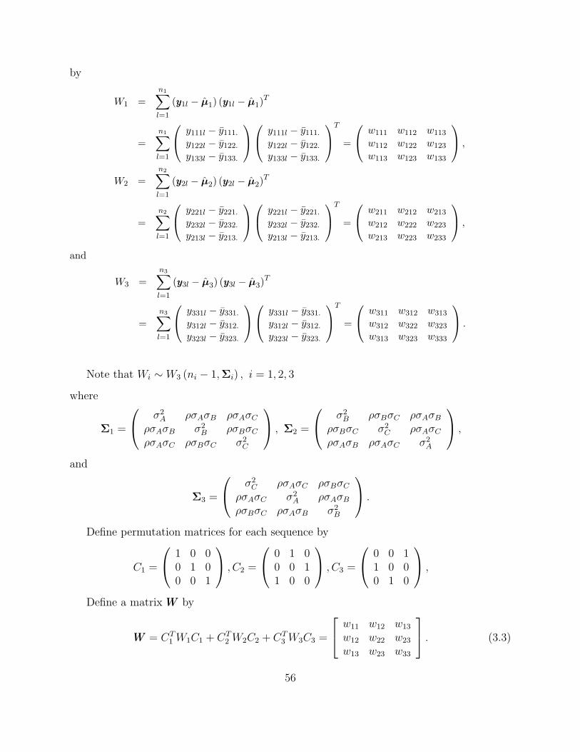
by
W1 =n1∑l=1
(yy1l − µ1) (yy1l − µ1)T
=n1∑l=1
y111l − y111.
y122l − y122.
y133l − y133.
y111l − y111.
y122l − y122.
y133l − y133.
T
=
w111 w112 w113
w112 w122 w123
w113 w123 w133
,
W2 =n2∑l=1
(yy2l − µ2) (yy2l − µ2)T
=n2∑l=1
y221l − y221.
y232l − y232.
y213l − y213.
y221l − y221.
y232l − y232.
y213l − y213.
T
=
w211 w212 w213
w212 w222 w223
w213 w223 w233
,
and
W3 =n3∑l=1
(yy3l − µ3) (yy3l − µ3)T
=n3∑l=1
y331l − y331.
y312l − y312.
y323l − y323.
y331l − y331.
y312l − y312.
y323l − y323.
T
=
w311 w312 w313
w312 w322 w323
w313 w323 w333
.
Note that Wi ∼ W3 (ni − 1,Σi) , i = 1, 2, 3
where
Σ1 =
σ2A ρσAσB ρσAσC
ρσAσB σ2B ρσBσC
ρσAσC ρσBσC σ2C
, Σ2 =
σ2B ρσBσC ρσAσB
ρσBσC σ2C ρσAσC
ρσAσB ρσAσC σ2A
,
and
Σ3 =
σ2C ρσAσC ρσBσC
ρσAσC σ2A ρσAσB
ρσBσC ρσAσB σ2B
.
Define permutation matrices for each sequence by
C1 =
1 0 00 1 00 0 1
, C2 =
0 1 00 0 11 0 0
, C3 =
0 0 11 0 00 1 0
,
Define a matrix WW by
WW = CT1 W1C1 + CT
2 W2C2 + CT3 W3C3 =
w11 w12 w13
w12 w22 w23
w13 w23 w33
. (3.3)
56

Note that
cov(CTi εεil
)= Σ, i = 1, 2, 3, l = 1, 2, · · · , ni
where
Σ =
σ2A ρσAσB ρσAσC
ρσAσB σ2B ρσBσC
ρσAσC ρσBσC σ2C
.
Thus WW ∼ W (N−3,Σ) where N = n1+n2+n3 and Σ =
σ2A ρσAσB ρσAσC
ρσAσB σ2B ρσBσC
ρσAσC ρσBσC σ2C
.
LetD1/2 = diag(σA, σB, σC) and R =
1 ρ ρρ 1 ρρ ρ 1
, then it is noted that Σ = D1/2RD1/2.
The inverse of Σ is given by
Σ−1 = D−1/2R−1D−1/2
where
D−1/2 = diag
(1
σA,
1
σB,
1
σC
)and R−1 =
1
(1− ρ)(1 + 2ρ)
1 + ρ −ρ −ρ−ρ 1 + ρ −ρ−ρ −ρ 1 + ρ
.
Consider testing H0 : σ2A = σ2
B = σ2C versus HA : not H0. The likelihood function is
given by
L(Σ) = c|WW |N−7
2 exp(
12tr(WWΣ−1
))|Σ|N−3
2
where
c =1
23(N−3)/2π3/2
3∏i=1
Γ
(N − (i+ 2)
2
) and N =3∑i=1
ni.
The log-likelihood function is
log (L(Σ)) = log(c) +N − 7
2log|WW | − N − 3
2log|Σ| − 1
2tr(WWΣ−1
).
57

Under H0 : σ2A = σ2
B = σ2C = σ2, one has
|Σ| = σ6(1− ρ)2(1 + 2ρ)
and
tr(WWΣ−1
)=
(1 + ρ)(w11 + w22 + w33)
(1− ρ)2(1 + 2ρ)σ2− 2ρ(w12 + w13 + w23)
(1− ρ)2(1 + 2ρ)σ2.
The log-likelihood function under restricted condition, H0, is
log (L(Σ)) = log(c) +N − 7
2log|WW | − N − 3
2
[3logσ2 + log
((1− ρ)2(1 + 2ρ)
)]−(1 + ρ)(w11 + w22 + w33)
2(1− ρ)2(1 + 2ρ)σ2+ρ(w12 + w13 + w23)
(1− ρ)2(1 + 2ρ)σ2.
The derivatives of logL(Σ) with respect to σ2 and ρ are as follows:
∂logL(Σ)
∂σ2= −3(N − 3)
2σ2+
(1 + ρ)(w11 + w22 + w33)− 2ρ(w12 + w13 + w23)
2(1− ρ)(1 + 2ρ)σ4,
∂logL(Σ)
∂ρ=
3(N − 3)ρ
(1− ρ)(1 + 2ρ)− ρ(2 + ρ)(w11 + w22 + w33)
(1− ρ)2(1 + 2ρ)2σ2+
(1 + 2ρ2)(w12 + w13 + w23)
(1− ρ)2(1 + 2ρ)2σ2.
Setting the derivatives of logL(Σ) with respect to σ2 and ρ equal to zero, one gets
3(N − 3)σ2 − (1 + ρ)(w11 + w22 + w33)− 2ρ(w12 + w13 + w23)
(1− ρ)(1 + 2ρ)= 0,
3(N − 3)ρ(1− ρ)(1 + 2ρ)−(w11 + w22 + w33
σ2
)ρ(2 + ρ) +
(w12 + w13 + w23
σ2
)(1 + 2ρ2) = 0.
Under restricted condition, the parameter estimators are
σ2R =
w11 + w22 + w33
3(N − 3)and ρ =
w12 + w13 + w23
w11 + w22 + w33
.
Thus, the method of moment estimators and the maximum likelihood estimators are
identical.
Under HA : not H0, one has
|Σ| = σ2Aσ
2Bσ
2C(1− ρ)2(1 + 2ρ)
58
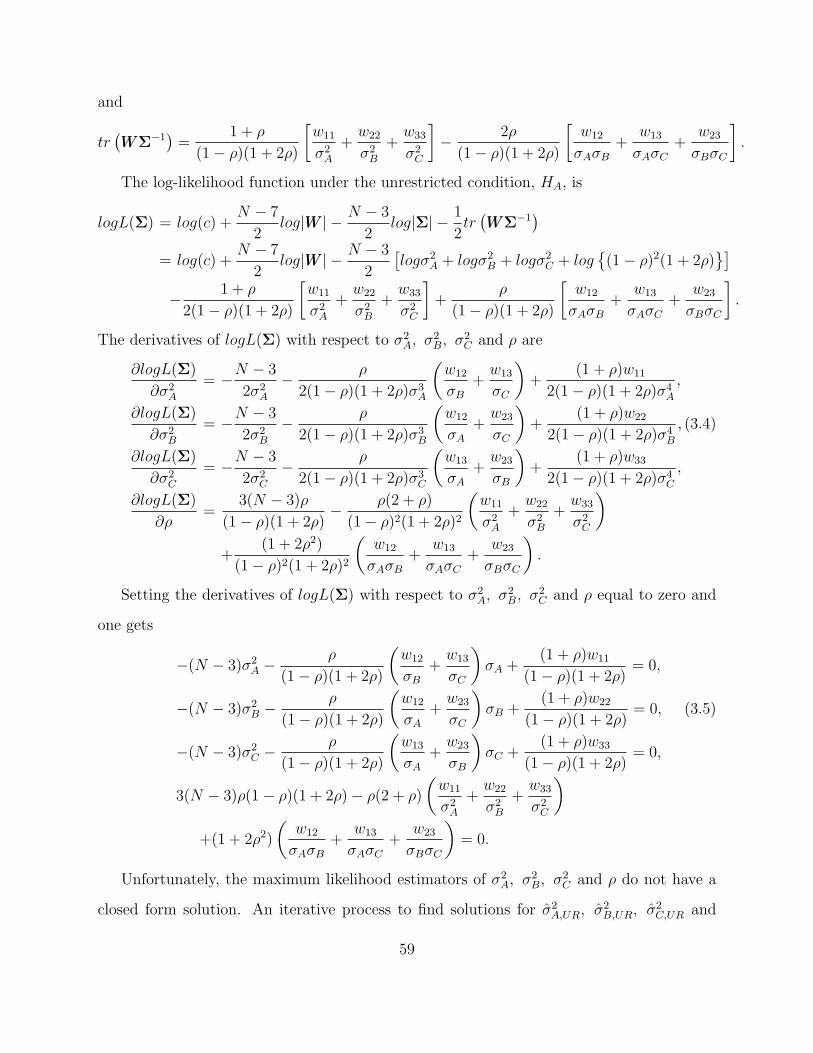
and
tr(WWΣ−1
)=
1 + ρ
(1− ρ)(1 + 2ρ)
[w11
σ2A
+w22
σ2B
+w33
σ2C
]− 2ρ
(1− ρ)(1 + 2ρ)
[w12
σAσB+
w13
σAσC+
w23
σBσC
].
The log-likelihood function under the unrestricted condition, HA, is
logL(Σ) = log(c) +N − 7
2log|WW | − N − 3
2log|Σ| − 1
2tr(WWΣ−1
)= log(c) +
N − 7
2log|WW | − N − 3
2
[logσ2
A + logσ2B + logσ2
C + log{
(1− ρ)2(1 + 2ρ)}]
− 1 + ρ
2(1− ρ)(1 + 2ρ)
[w11
σ2A
+w22
σ2B
+w33
σ2C
]+
ρ
(1− ρ)(1 + 2ρ)
[w12
σAσB+
w13
σAσC+
w23
σBσC
].
The derivatives of logL(Σ) with respect to σ2A, σ
2B, σ
2C and ρ are
∂logL(Σ)
∂σ2A
= −N − 3
2σ2A
− ρ
2(1− ρ)(1 + 2ρ)σ3A
(w12
σB+w13
σC
)+
(1 + ρ)w11
2(1− ρ)(1 + 2ρ)σ4A
,
∂logL(Σ)
∂σ2B
= −N − 3
2σ2B
− ρ
2(1− ρ)(1 + 2ρ)σ3B
(w12
σA+w23
σC
)+
(1 + ρ)w22
2(1− ρ)(1 + 2ρ)σ4B
, (3.4)
∂logL(Σ)
∂σ2C
= −N − 3
2σ2C
− ρ
2(1− ρ)(1 + 2ρ)σ3C
(w13
σA+w23
σB
)+
(1 + ρ)w33
2(1− ρ)(1 + 2ρ)σ4C
,
∂logL(Σ)
∂ρ=
3(N − 3)ρ
(1− ρ)(1 + 2ρ)− ρ(2 + ρ)
(1− ρ)2(1 + 2ρ)2
(w11
σ2A
+w22
σ2B
+w33
σ2C
)+
(1 + 2ρ2)
(1− ρ)2(1 + 2ρ)2
(w12
σAσB+
w13
σAσC+
w23
σBσC
).
Setting the derivatives of logL(Σ) with respect to σ2A, σ
2B, σ
2C and ρ equal to zero and
one gets
−(N − 3)σ2A −
ρ
(1− ρ)(1 + 2ρ)
(w12
σB+w13
σC
)σA +
(1 + ρ)w11
(1− ρ)(1 + 2ρ)= 0,
−(N − 3)σ2B −
ρ
(1− ρ)(1 + 2ρ)
(w12
σA+w23
σC
)σB +
(1 + ρ)w22
(1− ρ)(1 + 2ρ)= 0, (3.5)
−(N − 3)σ2C −
ρ
(1− ρ)(1 + 2ρ)
(w13
σA+w23
σB
)σC +
(1 + ρ)w33
(1− ρ)(1 + 2ρ)= 0,
3(N − 3)ρ(1− ρ)(1 + 2ρ)− ρ(2 + ρ)
(w11
σ2A
+w22
σ2B
+w33
σ2C
)+(1 + 2ρ2)
(w12
σAσB+
w13
σAσC+
w23
σBσC
)= 0.
Unfortunately, the maximum likelihood estimators of σ2A, σ
2B, σ
2C and ρ do not have a
closed form solution. An iterative process to find solutions for σ2A,UR, σ
2B,UR, σ
2C,UR and
59
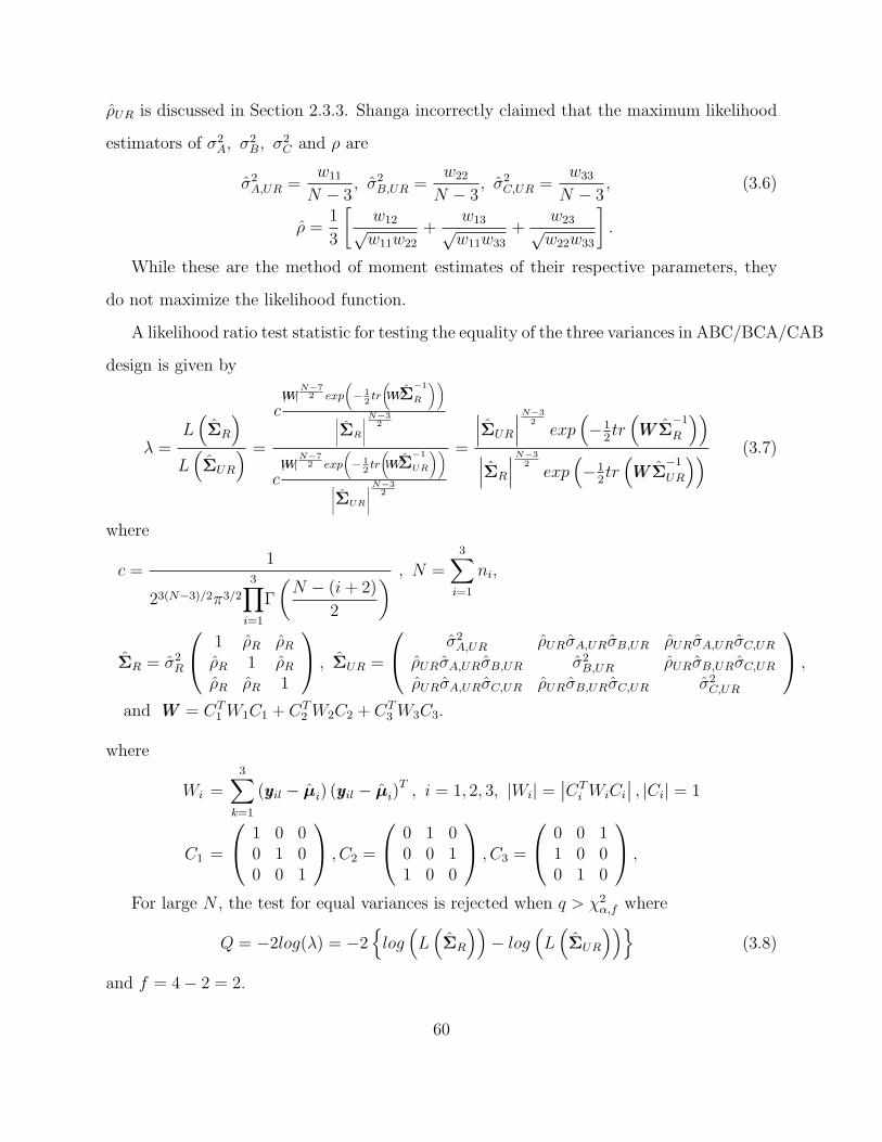
ρUR is discussed in Section 2.3.3. Shanga incorrectly claimed that the maximum likelihood
estimators of σ2A, σ
2B, σ
2C and ρ are
σ2A,UR =
w11
N − 3, σ2
B,UR =w22
N − 3, σ2
C,UR =w33
N − 3, (3.6)
ρ =1
3
[w12√w11w22
+w13√w11w33
+w23√w22w33
].
While these are the method of moment estimates of their respective parameters, they
do not maximize the likelihood function.
A likelihood ratio test statistic for testing the equality of the three variances in ABC/BCA/CAB
design is given by
λ =L(ΣR
)L(ΣUR
) =
c|WW |
N−72 exp
(− 1
2tr
(WW
ˆΣ−1
R
))∣∣∣∣ ˆΣR
∣∣∣∣N−32
c|WW |
N−72 exp
(− 1
2tr
(WW
ˆΣ−1
UR
))∣∣∣∣ ˆΣUR
∣∣∣∣N−32
=
∣∣∣ΣUR
∣∣∣N−32exp
(−1
2tr(WW Σ
−1
R
))∣∣∣ΣR
∣∣∣N−32exp
(−1
2tr(WW Σ
−1
UR
)) (3.7)
where
c =1
23(N−3)/2π3/2
3∏i=1
Γ
(N − (i+ 2)
2
) , N =3∑i=1
ni,
ΣR = σ2R
1 ρR ρRρR 1 ρRρR ρR 1
, ΣUR =
σ2A,UR ρURσA,URσB,UR ρURσA,URσC,UR
ρURσA,URσB,UR σ2B,UR ρURσB,URσC,UR
ρURσA,URσC,UR ρURσB,URσC,UR σ2C,UR
,
and WW = CT1 W1C1 + CT
2 W2C2 + CT3 W3C3.
where
Wi =3∑
k=1
(yyil − µi) (yyil − µi)T , i = 1, 2, 3, |Wi| =
∣∣CTi WiCi
∣∣ , |Ci| = 1
C1 =
1 0 00 1 00 0 1
, C2 =
0 1 00 0 11 0 0
, C3 =
0 0 11 0 00 1 0
,
For large N , the test for equal variances is rejected when q > χ2α,f where
Q = −2log(λ) = −2{log(L(ΣR
))− log
(L(ΣUR
))}(3.8)
and f = 4− 2 = 2.
60

3.3 Methods for Estimating Parameters
Since, under the unrestricted condition in the (ABC/BCA/CAB) design, solutions of
σ2A, σ
2B, σ
2C and ρ for this design do not have a closed form, one needs to consider other
methods to find the maximum likelihood estimators under HA.
Consider the derivatives of the log-likelihood functions from (3.4):
∂logL(Σ)
∂σ2A
= −N − 3
2σ2A
− ρ
2(1− ρ)(1 + 2ρ)σ3A
(w12
σB+w13
σC
)+
(1 + ρ)w11
2(1− ρ)(1 + 2ρ)σ4A
,
∂logL(Σ)
∂σ2B
= −N − 3
2σ2B
− ρ
2(1− ρ)(1 + 2ρ)σ3B
(w12
σA+w23
σC
)+
(1 + ρ)w22
2(1− ρ)(1 + 2ρ)σ4B
, (3.9)
∂logL(Σ)
∂σ2C
= −N − 3
2σ2C
− ρ
2(1− ρ)(1 + 2ρ)σ3C
(w13
σA+w23
σB
)+
(1 + ρ)w33
2(1− ρ)(1 + 2ρ)σ4C
,
∂logL(Σ)
∂ρ=
3(N − 3)ρ
(1− ρ)(1 + 2ρ)− ρ(2 + ρ)
(1− ρ)2(1 + 2ρ)2
(w11
σ2A
+w22
σ2B
+w33
σ2C
)+
(1 + 2ρ2)
(1− ρ)2(1 + 2ρ)2
(w12
σAσB+
w13
σAσC+
w23
σBσC
).
Setting the derivatives of logL(Σ) with respect to σ2A, σ
2B, σ
2C and ρ equal to zero and
one can get:
−(N − 3)σ2A −
ρ
(1− ρ)(1 + 2ρ)
(w12
σB+w13
σC
)σA +
(1 + ρ)w11
(1− ρ)(1 + 2ρ)= 0,
−(N − 3)σ2B −
ρ
(1− ρ)(1 + 2ρ)
(w12
σA+w23
σC
)σB +
(1 + ρ)w22
(1− ρ)(1 + 2ρ)= 0, (3.10)
−(N − 3)σ2C −
ρ
(1− ρ)(1 + 2ρ)
(w13
σA+w23
σB
)σC +
(1 + ρ)w33
(1− ρ)(1 + 2ρ)= 0,
3(N − 3)ρ(1− ρ)(1 + 2ρ)− ρ(2 + ρ)
(w11
σ2A
+w22
σ2B
+w33
σ2C
)+(1 + 2ρ2)
(w12
σAσB+
w13
σAσC+
w23
σBσC
)= 0.
Note that the first three equations in (3.10) are quadratic functions of σA, σB and σC ,
respectively, and the fourth equation is a cubic function of ρ. The theorem 2 and 3 can be
applied to estimate the parameters, σA, σB, σC and ρ.
The following iterative procedure can be used to find the maximum likelihood estimates
of σA, σB, σC and ρ.
61

Procedure
1. Set starting values using the method of moment estimates from (3.6):
σ0A =
√σ2A,UR, σ
0B =
√σ2B,UR, σ
0C =
√σ2C,UR, and ρ0 = ρUR
where σ2A,UR =
w11
N − 3, σ2
B,UR =w22
N − 3, σ2
C,UR =w33
N − 3,
ρ =1
3
[w12√w11w22
+w13√w11w33
+w23√w22w33
].
2. Plug σ0B, σ
0C , and ρ0 into the quadratic equation of σA:
− (N − 3)σ2A −
ρ0
(1− ρ0)(1 + 2ρ0)
(w12
σ0B
+w13
σ0C
)σA +
(1 + ρ0)w11
(1− ρ0)(1 + 2ρ0)= 0
And obtain a solution for the parameter, σA by using Definition 2: call the solution,
σA.
3. Plug σA, σ0C , and ρ0 into the quadratic equation of σB:
− (N − 3)σ2B −
ρ0
(1− ρ0)(1 + 2ρ0)
(w12
σA+w23
σ0C
)σB +
(1 + ρ0)w22
(1− ρ0)(1 + 2ρ0)= 0
And obtain a solution for the parameter, σB by using Definition 2: call the solution,
σB.
4. Plug σA, σB, and ρ0 into the quadratic equations of σC :
− (N − 3)σ2C −
ρ0
(1− ρ0)(1 + 2ρ0)
(w13
σA+w23
σB
)σC +
(1 + ρ0)w33
(1− ρ0)(1 + 2ρ0)= 0
And obtain a solution for the parameter, σC by using Definition 2: call the solution,
σC .
5. Plug σA, σB, and σC into the cubic equation of ρ:
3(N − 3)ρ(1− ρ)(1 + 2ρ)− ρ(2 + ρ)
(w11
σ2A
+w22
σ2B
+w33
σ2C
)+(1 + 2ρ2)
(w12
σAσB+
w13
σAσC+
w23
σBσC
)= 0.
And obtain a solution for the parameter, ρ, by using Definition 3: call the solution, ρ.
62

6. If |σA − σ0A| < ε, |σB − σ0
B| < ε, |σC − σ0C | < ε, and |ρ− ρ0| < ε where ε = 10−5, then
STOP and use σA, σB, σC , and ρ as maximum likelihood estimates of σA, σB, σC ,
and ρ.
If |σA − σ0A| > ε or |σB − σ0
B| > ε or |σC − σ0C | > ε or |ρ− ρ0| > ε, repeat steps 2-5
with σ0A ← σA, σ
0B ← σB, σ
0C ← σC , and ρ0 ← ρ.
The following section considers the performance of the proposed method to obtain the
likelihood ratio test statistics.
63
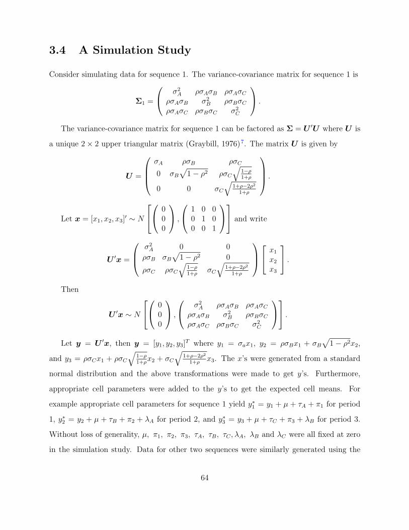
3.4 A Simulation Study
Consider simulating data for sequence 1. The variance-covariance matrix for sequence 1 is
Σ1 =
σ2A ρσAσB ρσAσC
ρσAσB σ2B ρσBσC
ρσAσC ρσBσC σ2C
.
The variance-covariance matrix for sequence 1 can be factored as Σ = U ′U where U is
a unique 2× 2 upper triangular matrix (Graybill, 1976)7. The matrix U is given by
U =
σA ρσB ρσC
0 σB√
1− ρ2 ρσC
√1−ρ1+ρ
0 0 σC
√1+ρ−2ρ2
1+ρ
.
Let x = [x1, x2, x3]′ ∼ N
000
,
1 0 00 1 00 0 1
and write
U ′x =
σ2A 0 0
ρσB σB√
1− ρ2 0
ρσC ρσC
√1−ρ1+ρ
σC
√1+ρ−2ρ2
1+ρ
x1
x2
x3
.Then
U ′x ∼ N
000
,
σ2A ρσAσB ρσAσC
ρσAσB σ2B ρσBσC
ρσAσC ρσBσC σ2C
.Let y = U ′x, then y = [y1, y2, y3]
T where y1 = σax1, y2 = ρσBx1 + σB√
1− ρ2x2,
and y3 = ρσCx1 + ρσC
√1−ρ1+ρ
x2 + σC
√1+ρ−2ρ2
1+ρx3. The x’s were generated from a standard
normal distribution and the above transformations were made to get y’s. Furthermore,
appropriate cell parameters were added to the y’s to get the expected cell means. For
example appropriate cell parameters for sequence 1 yield y∗1 = y1 + µ + τA + π1 for period
1, y∗2 = y2 + µ + τB + π2 + λA for period 2, and y∗3 = y3 + µ + τC + π3 + λB for period 3.
Without loss of generality, µ, π1, π2, π3, τA, τB, τC , λA, λB and λC were all fixed at zero
in the simulation study. Data for other two sequences were similarly generated using the
64
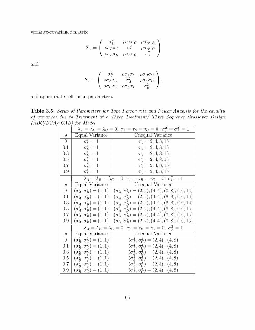
variance-covariance matrix
Σ2 =
σ2B ρσBσC ρσAσB
ρσBσC σ2C ρσAσC
ρσAσB ρσAσC σ2A
and
Σ3 =
σ2C ρσAσC ρσBσC
ρσAσC σ2A ρσAσB
ρσBσC ρσAσB σ2B
.
and appropriate cell mean parameters.
Table 3.5: Setup of Parameters for Type I error rate and Power Analysis for the equalityof variances due to Treatment at a Three Treatment/ Three Sequence Crossover Design(ABC/BCA/ CAB) for Model
λA = λB = λC = 0, τA = τB = τC = 0, σ2A = σ2
B = 1ρ Equal Variance Unequal Variance0 σ2
C = 1 σ2C = 2, 4, 8, 16
0.1 σ2C = 1 σ2
C = 2, 4, 8, 160.3 σ2
C = 1 σ2C = 2, 4, 8, 16
0.5 σ2C = 1 σ2
C = 2, 4, 8, 160.7 σ2
C = 1 σ2C = 2, 4, 8, 16
0.9 σ2C = 1 σ2
C = 2, 4, 8, 16
λA = λB = λC = 0, τA = τB = τC = 0, σ2C = 1
ρ Equal Variance Unequal Variance0 (σ2
A, σ2B) = (1, 1) (σ2
A, σ2B) = (2, 2), (4, 4), (8, 8), (16, 16)
0.1 (σ2A, σ
2B) = (1, 1) (σ2
A, σ2B) = (2, 2), (4, 4), (8, 8), (16, 16)
0.3 (σ2A, σ
2B) = (1, 1) (σ2
A, σ2B) = (2, 2), (4, 4), (8, 8), (16, 16)
0.5 (σ2A, σ
2B) = (1, 1) (σ2
A, σ2B) = (2, 2), (4, 4), (8, 8), (16, 16)
0.7 (σ2A, σ
2B) = (1, 1) (σ2
A, σ2B) = (2, 2), (4, 4), (8, 8), (16, 16)
0.9 (σ2A, σ
2B) = (1, 1) (σ2
A, σ2B) = (2, 2), (4, 4), (8, 8), (16, 16)
λA = λB = λC = 0, τA = τB = τC = 0, σ2A = 1
ρ Equal Variance Unequal Variance0 (σ2
B, σ2C) = (1, 1) (σ2
B, σ2C) = (2, 4), (4, 8)
0.1 (σ2B, σ
2C) = (1, 1) (σ2
B, σ2C) = (2, 4), (4, 8)
0.3 (σ2B, σ
2C) = (1, 1) (σ2
B, σ2C) = (2, 4), (4, 8)
0.5 (σ2B, σ
2C) = (1, 1) (σ2
B, σ2C) = (2, 4), (4, 8)
0.7 (σ2B, σ
2C) = (1, 1) (σ2
B, σ2C) = (2, 4), (4, 8)
0.9 (σ2B, σ
2C) = (1, 1) (σ2
B, σ2C) = (2, 4), (4, 8)
65

Consider the likelihood ratio test of the three treatment crossover design when treatments
have unequal variances. Table 3.5 shows the parameters that were used when simulating
data for Type I error rate and power analyses for testing the equality of variances due to
treatments. To get the empirical Type I error rates and the power, 1000 simulations were
done for each n, ρ, σ2A, σ
2B and σ2
C .
To estimate parameters, the proposed method mentioned in Section 2.2 is used in R.
And, with the same data generated in R, the likelihood ratio tests using SAS-MIXED to
calculate Type I error rates and powers are obtained using the following SAS commands.
Step 1 Import data
INFILE ’C:\Data\KSU PhD THESIS\PRG\y12-148data.txt’ DELIMITER=’ ’;
INPUT rho sA2 sB2 sC2 nsubj sim seq subj y1 y2 y3;
Step 2 Define periods and arrange treatments
DATA one; SET one;
DROP y1 y2 y3;
per=1; y=y1; output;
per=2; y=y2; output;
per=3; y=y3; output;
RUN;
DATA one; SET one;
SUbJ=subj+(seq-1)*nsubj;
trt=’A’;
IF seq=1 and per=2 THEN trt=’B’;
IF seq=1 and per=3 THEN trt=’C’;
IF seq=2 and per=1 THEN trt=’B’;
IF seq=2 and per=2 THEN trt=’C’;
IF seq=3 and per=1 THEN trt=’C’;
66

IF seq=3 and per=3 THEN trt=’B’;
RUN;
Step 3 Calculate −2log(L(ΣR
))in (3.8)
PROC MIXED ic data=one;
TITLE ’ANALYSIS USING SAS-MIXED’;
by rho sim;
CLASSES seq per trt subj;
MODEL y=seq trt per/DDFM=SATTERTH;
REPEATED trt/ SUBJECT=subj TYPE=CS;
ods listing exclude all;
ods output infocrit = null COVPARMS=HOPARMS;
RUN;
DATA null; set null;
rename neg2loglike =ho;
drop aic--caic;
Step 4 Calculate −2log(L(ΣUR
))in (3.8)
PROC MIXED ic data=one;
TITLE ’ANALYSIS USING SAS-MIXED’;
by rho sim;
CLASSES seq per trt subj;
MODEL y=seq trt per/DDFM=SATTERTH;
REPEATED trt/ SUBJECT=subj TYPE=CSH;
ods listing exclude all;
ods output infocrit = ha COVPARMS=HAPARMS;
RUN;
67

DATA ha; set ha;
rename neg2loglike =ha;
drop aic--caic;
Step 5 Calculate the Type I error rate
DATA comb; SET comb;
u = ho-ha;
IF u>5.991465 THEN reject=1; ELSE reject=0;
RUN;
PROC MEANS data=comb;
by rho;
ods listing select all;
var reject;
RUN;
All of the SAS steps for the three treatment design are shown in Appendix F. Figure C.1
shows the Type I error rates of the likelihood ratio tests for H0 : σ2A = σ2
B = σ2C and
Table D.1 shows the observed Type I error of the likelihood ratio tests for H0 : σ2A =
σ2B = σ2
C . Figure C.1 has six lines. Each line corresponds to a different value of ρ, ρ =
0.0, 0.1, 0.3, 0.5, 0.7, 0.9. Figure C.1 shows that the Type I error with different correlation
converge to 0.05 as the number of subjects in each sequence becomes large. Table D.1 shows
the observed Type I error rates of the likelihood ratio tests for H0 : σ2A = σ2
B = σ2C by both
R and SAS-MIXED. Each row for each method in Table D.1 corresponds to a different
value of ρ, ρ = 0.0, 0.1, 0.3, 0.5, 0.7, 0.9. Each column corresponds to a different number of
subjects assigned to each sequence. The likelihood ratio tests generally hold their size when
the number of subjects is at least 12 per sequence for each value of ρ. The two analyses
differ in their Type I error rates only when the number of subjects is 3 and correlation is 0,
0.1, 0.3, 0.5, and 0.7. When the value of correlation is 0.1 and 0.3, Type I error rate by R is
68

larger than SAS. In the case of that correlation is 0, 0.5, and 0.7, Type I error rate by SAS
is larger than R. In no case are the differences large enough to be of any concern.
Next consider data that were generated for the cases when σ2A = σ2
B = 1 and σ2C =
2, 4, 8, 16. Figure C.2 and Table D.2 show the observed power for each ρ and n when
σ2C = 2. As the number of subjects increase from 6 to 24, the power sharply increases
towards 1. Figures C.3-C.5 show the trends and Tables D.3-D.5 show the observed power
as σ2C increases. When σ2
C increases to 4, 8, and 16, the power sharply increases towards 1.
The power is close to 1 as the value of correlation become larger. In every case the power
increases as ρ increases.
Figures C.6-C.9 and Tables D.6-D.9 use data that were generated in the case of changing
the values of variances A and B and holding σ2C = 1. Figures C.6-C.9 show the trends and
Tables D.6-D.9 show the observed powers as σ2A and σ2
B increase. As the number of subjects
are increased from 6 to 24, the power is sharply increased towards 1. When the values of
variances A and B are increased to 4, 8, and 16, the power is sharply increased towards 1.
The final case is for data when all three variances are different. The trends are similar
to the two previous cases. See Figures C.10 and C.11, and Tables D.10 and D.11.
69
3.5 Conclusions
Data were generated for likelihood ratio test of equal variances for both the equal variance
case and the unequal variance case. The type I error rate results of the likelihood ratio test
for data with equal variance are shown in Figure C.1 and Table D.1. The power results of
the likelihood ratio tests for data with unequal variances are shown in Figures C.2-C.11,
and Tables D.2-D.11.
Generally, one needs at least 12 subjects per sequence to achieve acceptable Type I error
rates for each value of ρ. When one has at least 12 subjects per sequence, the power of the
likelihood ratio tests tend to increase as ρ increases.
It is important to note that while these simulation results were performed for the three
treatment/three period crossover design without carryover in a three sequence design, the
simulations performed using R are much more general than that. The simulations per-
formed using R were based on the sufficient statistics. In particular, they were based on the
distribution of WW defined in (3.4). Such a WW has a Wishart distribution whether there is
carryover or not. Also, if one should have the three treatment/three period crossover design
with or without carryover in a six sequence design, the distribution of WW will be Wishart
with degrees of freedom equal to N − 6 where N = n1 +n2 +n3 +n4 +n5 +n6. So the sim-
ulation results reported in Appendices C and D are valid for the six sequence design if one
views them as to the number of degrees of freedom associated with the underlying Wishart
distribution. For example, six subjects per sequence in the three sequence design will have
results similar to three subjects per sequence in the six sequence design as the former will
have 15 degrees of freedom for the Wishart distribution and the latter will have 12 degrees
of freedom for the Wishart distribution, and 9 subjects per sequence in a six sequence design
will perform similarly to 18 subjects per sequence in a three sequence design as the degrees
of freedom in the corresponding Wishart distributions are 48 and 51, respectively.
70

3.6 Future Work
In this chapter, crossover designs with data that have unequal variances are considered.
In particular, a crossover design having the number of treatments equal to the number
of periods (t = p = 3), ABC/BCA/CAB, was considered in this chapter. A constant
compound symmetry correlation structure under null hypothesis was considered.
As described in the previous section, the simulation results provided in this dissertation
can also be used to evaluate tests for equal variances when carryover is present and for the
Williams’ design for three treatments in three periods for the likelihood ratio tests based on
the Wishart distribution. However, analyses using SAS-MIXED in the three sequence de-
sign cannot be generalized to the carryover case nor to Williams’ designs. Simulations when
carryover is present in the six sequence three treatment Williams design using SAS-MIXED
should be obtained. Tests for equal variances should also be obtained for Williams’ de-
signs that involve more than three treatments using both SAS-MIXED and the appropriate
likelihood ratio test statistics.
All of the results in this dissertation assume that the underlying correlation structure for
the period measurements is compound symmetry. One should also consider other correlation
structures such as an autoregressive of lag 1 structure, a Toeplitz structure, or a banded
Toeplitz structure. In each of these cases, maximum likelihood estimators will need to be
obtained for both the null and alternative cases when one is basing tests on the appropriate
Wishart matrices.
Another topic for future study is to determine the robustness of these tests for equal
variances when the data are not normal.
71

Bibliography
[1] Balaam, L. N. (1968). A two-period design with t2 experimental units. Biometrics,
24:61–67.
[2] Brant, A. E. (1938). Tests of significance in reversal or switchback trials. Research
Bulletin, 234:Iowa agriculture experimental Station.
[3] Elfving, G. (1947). The asymptotical distribution of range in samples from a normal
population. Biometrika, 34:111–119.
[4] Fieller, E. C. (1940). The biological standardization of insulin (with discussion). Sup-
plement to the Journal of Royal Statistical Society, 7:1–64.
[5] Geisser, S. and Greenhouse, S. W. (1958). Extension of box’s results on the use of the f
distribution in multivariate analysis. Annals of Mathematical Statistics, 29:885–891.
[6] Goad, C. (1994). Multivariate and mixed models analysis of crossover designs with more
than two periods.
[7] Graybill, F. A. (1976). Theory and Application of the Linear Model. Duxbury Press:
North Scituate, Massachusetts.
[8] Greenhouse, S. W. and Geisser, S. (1959). On methods in the analysis of profile data.
Psychometrika, 24:95–112.
[9] Grizzle, J. E. (1965). The two-period changeover design and its use in clinical trials.
Biometrics, 21:467–480.
[10] Hsu, P. L. (1939). A new proof of thejoint product moment distribution. Proceedings
of the Cambridge Philosophical Society, 35:336.
72

[11] Hsu, P. L. (1940). On generalized analysis of variance. Biometrika, 31:221–237.
[12] Huynh, H. and Feldt, L. S. (1970). Condition under which mean square ratios in
repeated measurements design have exact f distributions. Journal of the American Sta-
tistical Association, 65(332):1582–1589.
[13] Huynh, H. and Feldt, L. S. (1976). Estimation of the box correction for degrees of
fredom from sample data in randomized block and split-plot designs. Journal of Education
Statistics, 1:69–82.
[14] Jambunathan, M. V. (1965). A quick method of deriving wishart’s distribution. Current
Series, 34:78.
[15] James, A. T. (1954). Normal multivariate analysis and the orthogonal group. Annals
of Mathematical Statistics, 25:40–75.
[16] Jones, B. and Kenward, M. (2003). Design and Analysis of Cross-Over Trials. London:
Chapman and Hall.
[17] Madow, W. G. (1938). Contributions to the theory of multivariate statistical analysis.
Trans. of the Amer. Math. Soc., 44:476.
[18] Mahalanobis, P. C., Bose, R. C., and Roy, S. N. (1937). Normalisation of statistical
variates and the use of rectangular co-ordinates in the theory of sampling distributions.
Sankhya, 3:1–40.
[19] Mardia, K. V., Kent, J. T., and Bibby, J. M. (1979). Multivariate Ananysis. California:
Academic Press.
[20] Matthews, J. N. (1988). Recent development in crossover design. International Statis-
tical Review, 56(2):117–127.
[21] Milliken, G. A. and Johnson, D. E. (1992). Ananysis of Messy Data. New York:
Chapman and Hill.
73

[22] Mood, A. M., Graybill, F. A., and Boes, D. C. (1974). Introduction to the Theory of
Statistics. McGraw-Hill, Inc: New York.
[23] Ogawa, I. and Roy, S. N. (1954). On multivariate distribution theory. Annals of
Mathematical Statistics, 25:329–339.
[24] Ogawa, J. (1953). On the sampling distributions of classical statistics in multivariate
analysis. Osaka Mathematical Journal, 5:13–52.
[25] Patterson, H. D. and Lucas, H. L. (1959). Extra-period change-over designs. Biometrics,
15:116–132.
[26] Rasch, G. (1948). A functional equation for wishart’s distribution. Annals of Mathe-
matical Statistics, 19:262–266.
[27] Ratkowsky, D. A., Evans, M. A., and Alldredge, J. R. (1993). Crossover Experiments,
Design, Analysis, and Application. New York: MArcel Dekker, Inc.
[28] Shanga, G. M. (2003). Analysis of crossover designs when treatments have unequal
variances.
[29] Sverdrup, E. (1947). Derivation of the wishart distribution of second order mements
by straight forward integration of a multiple integral. Skand. Aktuarietdskr., 30:151–166.
[30] Williams, E. J. (1949). Experimental designs balanced for the estimation of residual
effects of treatments. Australian Journal of Scientific Research, 2:149–164.
[31] Wishart, J. (1928). Sampling errors in the theory of two factors. British Journal of
Psychology, 19:180–187.
[32] Wishart, J. and Bartlett, M. S. (1933). The distribution of second order moment
statistics in a normal system. Proceedings of the Cambridge Philosophical Society, 28:455–
459.
74

Appendix A
Chapter 2: Figures for TwoTreatment Crossover Design
75
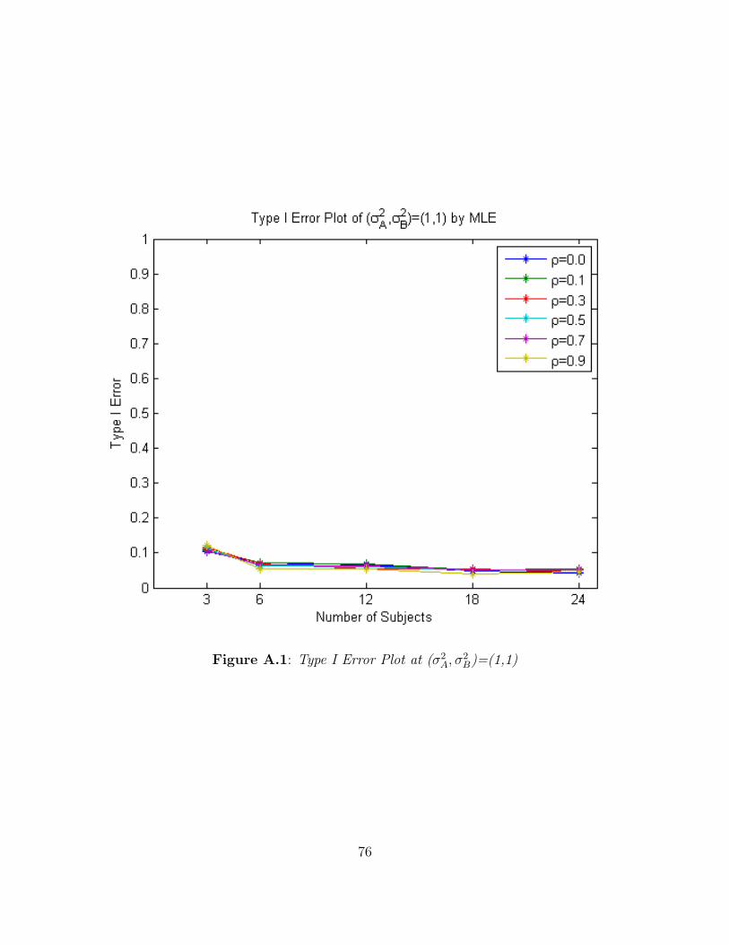
Figure A.1: Type I Error Plot at (σ2A, σ
2B)=(1,1)
76
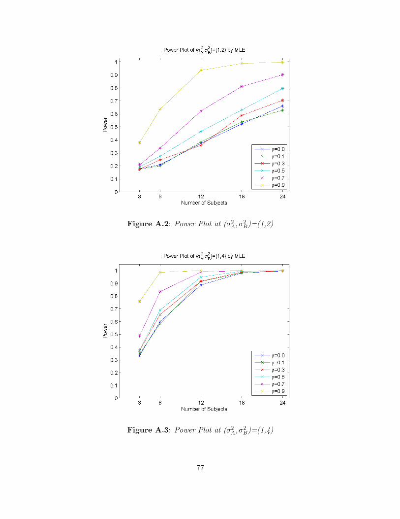
Figure A.2: Power Plot at (σ2A, σ
2B)=(1,2)
Figure A.3: Power Plot at (σ2A, σ
2B)=(1,4)
77
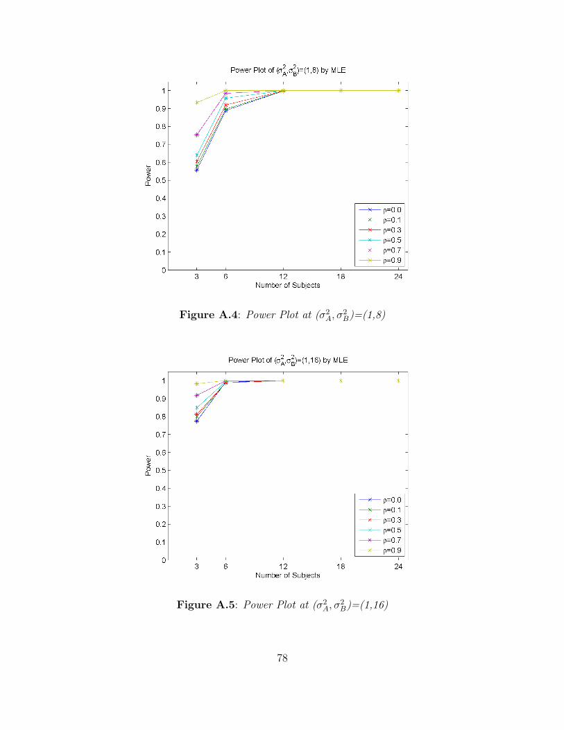
Figure A.4: Power Plot at (σ2A, σ
2B)=(1,8)
Figure A.5: Power Plot at (σ2A, σ
2B)=(1,16)
78

Appendix B
Chapter 2: Tables for Two TreatmentCrossover Design
79
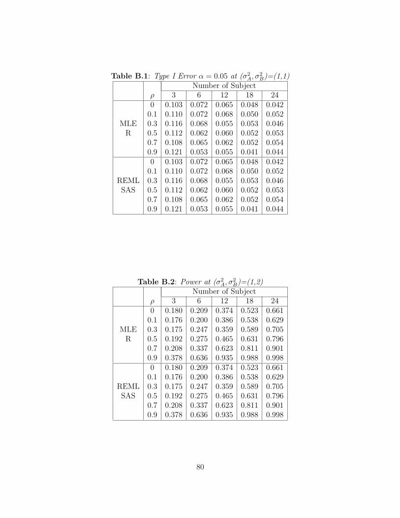
Table B.1: Type I Error α = 0.05 at (σ2A, σ
2B)=(1,1)
Number of Subjectρ 3 6 12 18 240 0.103 0.072 0.065 0.048 0.042
0.1 0.110 0.072 0.068 0.050 0.052MLE 0.3 0.116 0.068 0.055 0.053 0.046
R 0.5 0.112 0.062 0.060 0.052 0.0530.7 0.108 0.065 0.062 0.052 0.0540.9 0.121 0.053 0.055 0.041 0.0440 0.103 0.072 0.065 0.048 0.042
0.1 0.110 0.072 0.068 0.050 0.052REML 0.3 0.116 0.068 0.055 0.053 0.046SAS 0.5 0.112 0.062 0.060 0.052 0.053
0.7 0.108 0.065 0.062 0.052 0.0540.9 0.121 0.053 0.055 0.041 0.044
Table B.2: Power at (σ2A, σ
2B)=(1,2)
Number of Subjectρ 3 6 12 18 240 0.180 0.209 0.374 0.523 0.661
0.1 0.176 0.200 0.386 0.538 0.629MLE 0.3 0.175 0.247 0.359 0.589 0.705
R 0.5 0.192 0.275 0.465 0.631 0.7960.7 0.208 0.337 0.623 0.811 0.9010.9 0.378 0.636 0.935 0.988 0.9980 0.180 0.209 0.374 0.523 0.661
0.1 0.176 0.200 0.386 0.538 0.629REML 0.3 0.175 0.247 0.359 0.589 0.705SAS 0.5 0.192 0.275 0.465 0.631 0.796
0.7 0.208 0.337 0.623 0.811 0.9010.9 0.378 0.636 0.935 0.988 0.998
80
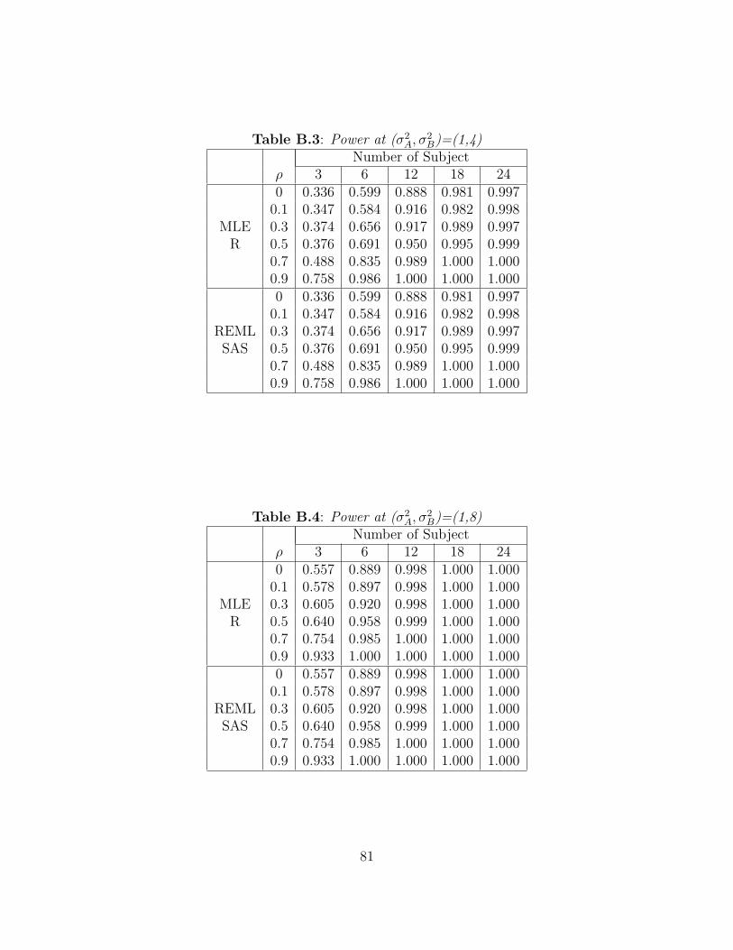
Table B.3: Power at (σ2A, σ
2B)=(1,4)
Number of Subjectρ 3 6 12 18 240 0.336 0.599 0.888 0.981 0.997
0.1 0.347 0.584 0.916 0.982 0.998MLE 0.3 0.374 0.656 0.917 0.989 0.997
R 0.5 0.376 0.691 0.950 0.995 0.9990.7 0.488 0.835 0.989 1.000 1.0000.9 0.758 0.986 1.000 1.000 1.0000 0.336 0.599 0.888 0.981 0.997
0.1 0.347 0.584 0.916 0.982 0.998REML 0.3 0.374 0.656 0.917 0.989 0.997SAS 0.5 0.376 0.691 0.950 0.995 0.999
0.7 0.488 0.835 0.989 1.000 1.0000.9 0.758 0.986 1.000 1.000 1.000
Table B.4: Power at (σ2A, σ
2B)=(1,8)
Number of Subjectρ 3 6 12 18 240 0.557 0.889 0.998 1.000 1.000
0.1 0.578 0.897 0.998 1.000 1.000MLE 0.3 0.605 0.920 0.998 1.000 1.000
R 0.5 0.640 0.958 0.999 1.000 1.0000.7 0.754 0.985 1.000 1.000 1.0000.9 0.933 1.000 1.000 1.000 1.0000 0.557 0.889 0.998 1.000 1.000
0.1 0.578 0.897 0.998 1.000 1.000REML 0.3 0.605 0.920 0.998 1.000 1.000SAS 0.5 0.640 0.958 0.999 1.000 1.000
0.7 0.754 0.985 1.000 1.000 1.0000.9 0.933 1.000 1.000 1.000 1.000
81
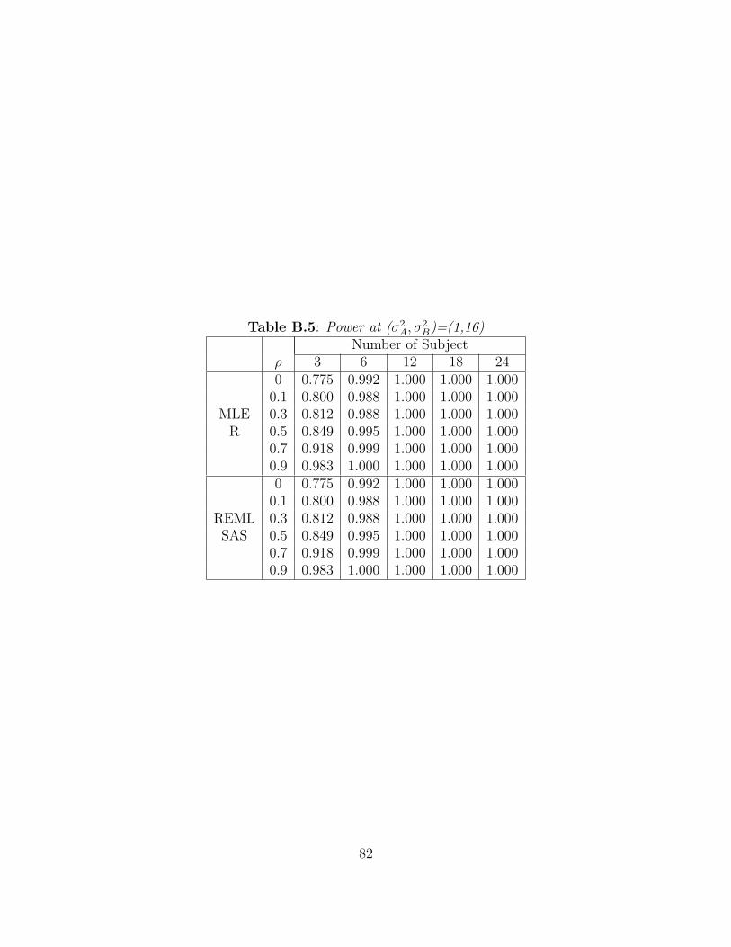
Table B.5: Power at (σ2A, σ
2B)=(1,16)
Number of Subjectρ 3 6 12 18 240 0.775 0.992 1.000 1.000 1.000
0.1 0.800 0.988 1.000 1.000 1.000MLE 0.3 0.812 0.988 1.000 1.000 1.000
R 0.5 0.849 0.995 1.000 1.000 1.0000.7 0.918 0.999 1.000 1.000 1.0000.9 0.983 1.000 1.000 1.000 1.0000 0.775 0.992 1.000 1.000 1.000
0.1 0.800 0.988 1.000 1.000 1.000REML 0.3 0.812 0.988 1.000 1.000 1.000SAS 0.5 0.849 0.995 1.000 1.000 1.000
0.7 0.918 0.999 1.000 1.000 1.0000.9 0.983 1.000 1.000 1.000 1.000
82

Appendix C
Chapter 3: Figures for ThreeTreatment Crossover Design
83
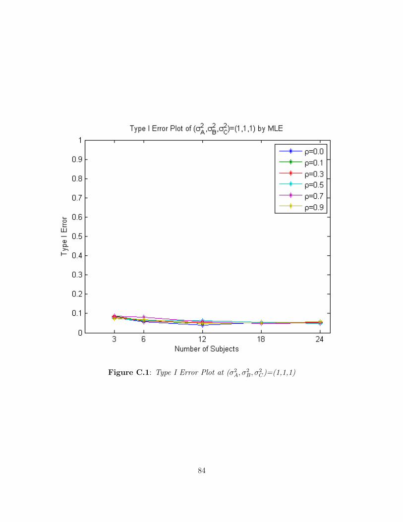
Figure C.1: Type I Error Plot at (σ2A, σ
2B, σ
2C)=(1,1,1)
84
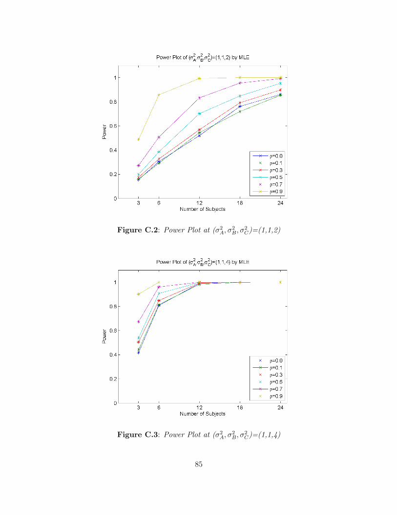
Figure C.2: Power Plot at (σ2A, σ
2B, σ
2C)=(1,1,2)
Figure C.3: Power Plot at (σ2A, σ
2B, σ
2C)=(1,1,4)
85
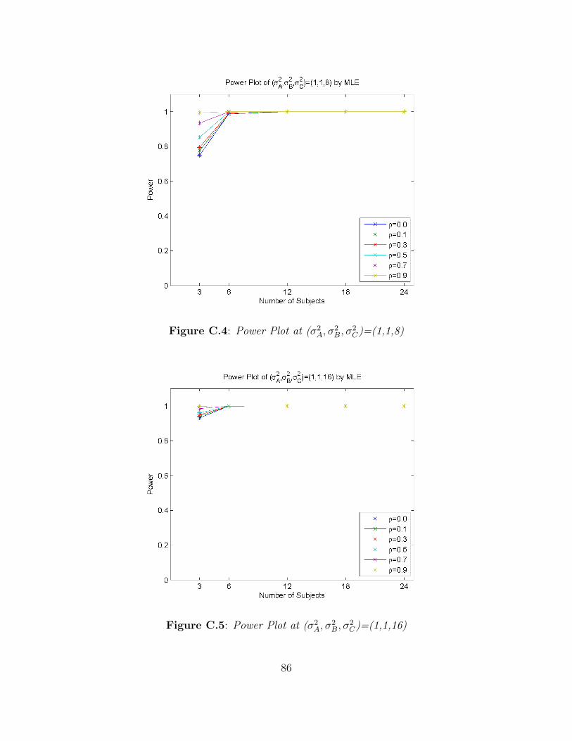
Figure C.4: Power Plot at (σ2A, σ
2B, σ
2C)=(1,1,8)
Figure C.5: Power Plot at (σ2A, σ
2B, σ
2C)=(1,1,16)
86
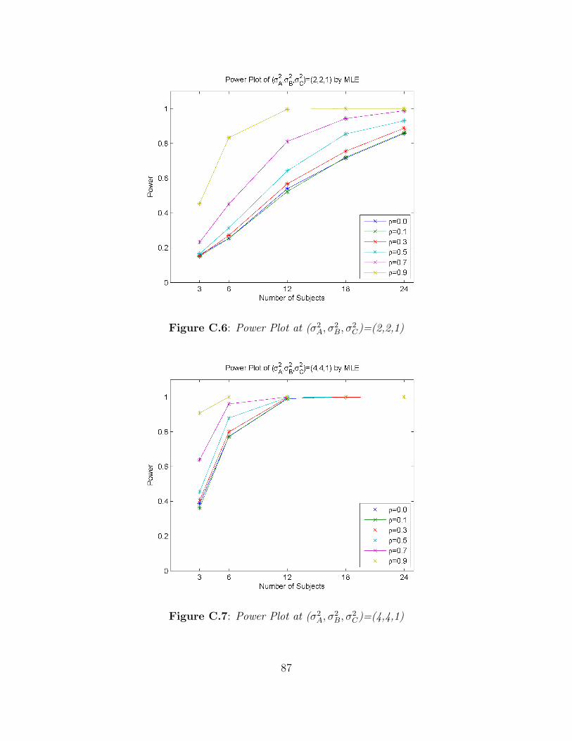
Figure C.6: Power Plot at (σ2A, σ
2B, σ
2C)=(2,2,1)
Figure C.7: Power Plot at (σ2A, σ
2B, σ
2C)=(4,4,1)
87
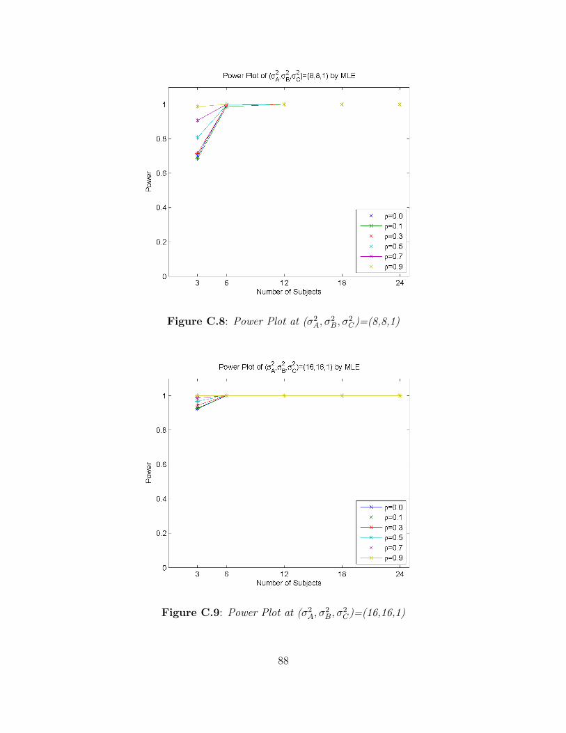
Figure C.8: Power Plot at (σ2A, σ
2B, σ
2C)=(8,8,1)
Figure C.9: Power Plot at (σ2A, σ
2B, σ
2C)=(16,16,1)
88
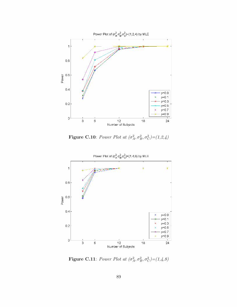
Figure C.10: Power Plot at (σ2A, σ
2B, σ
2C)=(1,2,4)
Figure C.11: Power Plot at (σ2A, σ
2B, σ
2C)=(1,4,8)
89

Appendix D
Chapter 3: Tables for ThreeTreatment Crossover Design
90
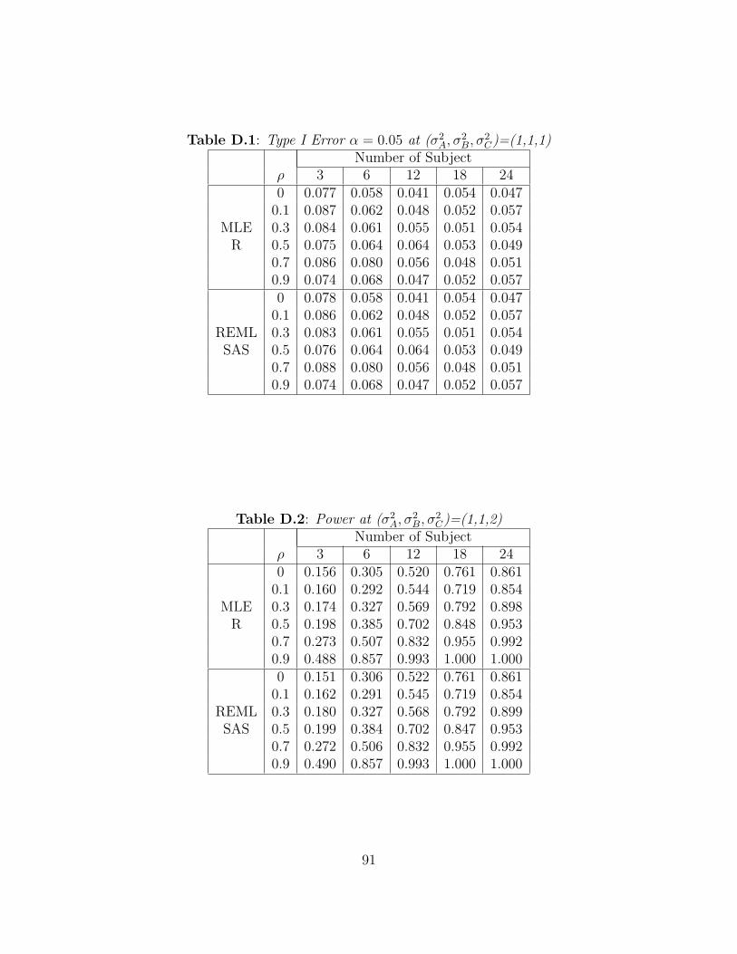
Table D.1: Type I Error α = 0.05 at (σ2A, σ
2B, σ
2C)=(1,1,1)
Number of Subjectρ 3 6 12 18 240 0.077 0.058 0.041 0.054 0.047
0.1 0.087 0.062 0.048 0.052 0.057MLE 0.3 0.084 0.061 0.055 0.051 0.054
R 0.5 0.075 0.064 0.064 0.053 0.0490.7 0.086 0.080 0.056 0.048 0.0510.9 0.074 0.068 0.047 0.052 0.0570 0.078 0.058 0.041 0.054 0.047
0.1 0.086 0.062 0.048 0.052 0.057REML 0.3 0.083 0.061 0.055 0.051 0.054SAS 0.5 0.076 0.064 0.064 0.053 0.049
0.7 0.088 0.080 0.056 0.048 0.0510.9 0.074 0.068 0.047 0.052 0.057
Table D.2: Power at (σ2A, σ
2B, σ
2C)=(1,1,2)
Number of Subjectρ 3 6 12 18 240 0.156 0.305 0.520 0.761 0.861
0.1 0.160 0.292 0.544 0.719 0.854MLE 0.3 0.174 0.327 0.569 0.792 0.898
R 0.5 0.198 0.385 0.702 0.848 0.9530.7 0.273 0.507 0.832 0.955 0.9920.9 0.488 0.857 0.993 1.000 1.0000 0.151 0.306 0.522 0.761 0.861
0.1 0.162 0.291 0.545 0.719 0.854REML 0.3 0.180 0.327 0.568 0.792 0.899SAS 0.5 0.199 0.384 0.702 0.847 0.953
0.7 0.272 0.506 0.832 0.955 0.9920.9 0.490 0.857 0.993 1.000 1.000
91
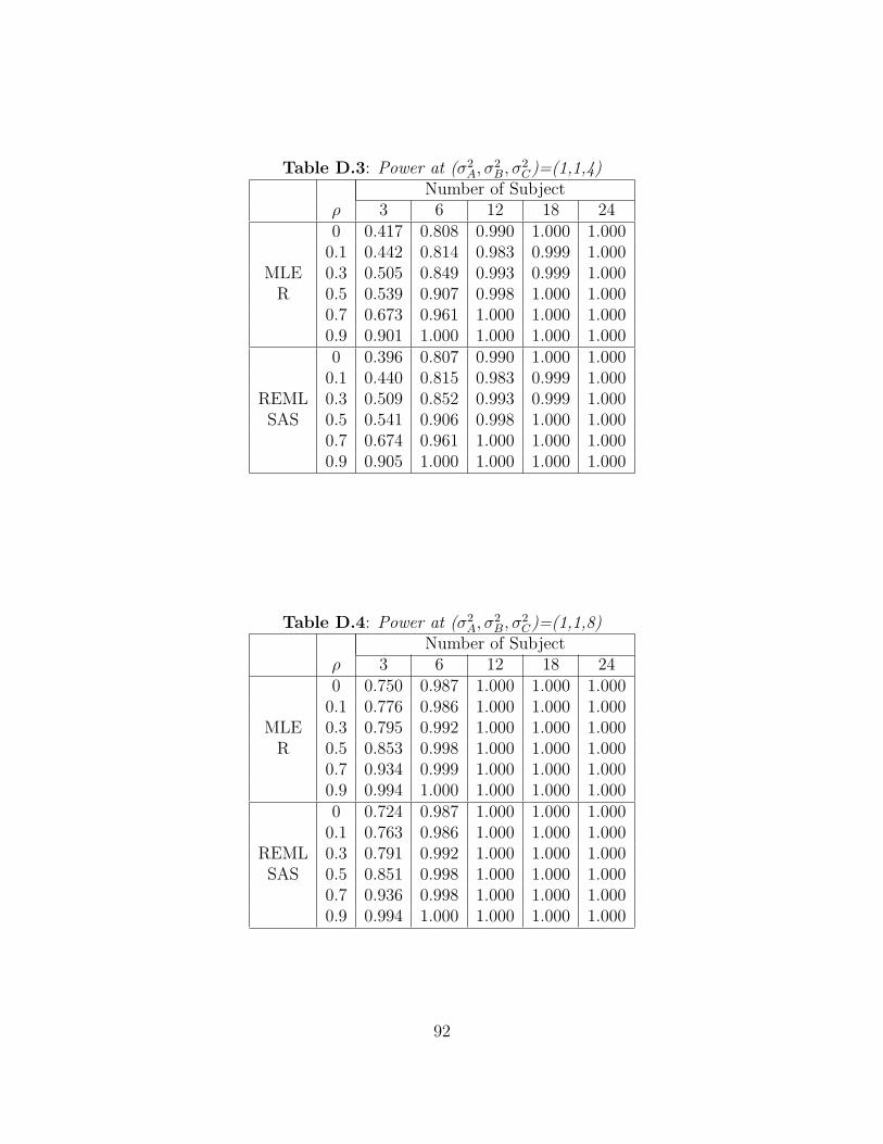
Table D.3: Power at (σ2A, σ
2B, σ
2C)=(1,1,4)
Number of Subjectρ 3 6 12 18 240 0.417 0.808 0.990 1.000 1.000
0.1 0.442 0.814 0.983 0.999 1.000MLE 0.3 0.505 0.849 0.993 0.999 1.000
R 0.5 0.539 0.907 0.998 1.000 1.0000.7 0.673 0.961 1.000 1.000 1.0000.9 0.901 1.000 1.000 1.000 1.0000 0.396 0.807 0.990 1.000 1.000
0.1 0.440 0.815 0.983 0.999 1.000REML 0.3 0.509 0.852 0.993 0.999 1.000SAS 0.5 0.541 0.906 0.998 1.000 1.000
0.7 0.674 0.961 1.000 1.000 1.0000.9 0.905 1.000 1.000 1.000 1.000
Table D.4: Power at (σ2A, σ
2B, σ
2C)=(1,1,8)
Number of Subjectρ 3 6 12 18 240 0.750 0.987 1.000 1.000 1.000
0.1 0.776 0.986 1.000 1.000 1.000MLE 0.3 0.795 0.992 1.000 1.000 1.000
R 0.5 0.853 0.998 1.000 1.000 1.0000.7 0.934 0.999 1.000 1.000 1.0000.9 0.994 1.000 1.000 1.000 1.0000 0.724 0.987 1.000 1.000 1.000
0.1 0.763 0.986 1.000 1.000 1.000REML 0.3 0.791 0.992 1.000 1.000 1.000SAS 0.5 0.851 0.998 1.000 1.000 1.000
0.7 0.936 0.998 1.000 1.000 1.0000.9 0.994 1.000 1.000 1.000 1.000
92
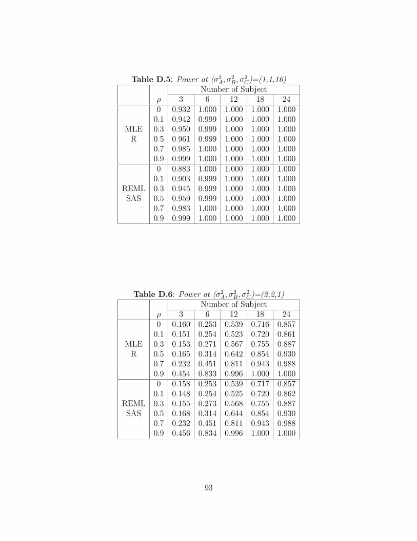
Table D.5: Power at (σ2A, σ
2B, σ
2C)=(1,1,16)
Number of Subjectρ 3 6 12 18 240 0.932 1.000 1.000 1.000 1.000
0.1 0.942 0.999 1.000 1.000 1.000MLE 0.3 0.950 0.999 1.000 1.000 1.000
R 0.5 0.961 0.999 1.000 1.000 1.0000.7 0.985 1.000 1.000 1.000 1.0000.9 0.999 1.000 1.000 1.000 1.0000 0.883 1.000 1.000 1.000 1.000
0.1 0.903 0.999 1.000 1.000 1.000REML 0.3 0.945 0.999 1.000 1.000 1.000SAS 0.5 0.959 0.999 1.000 1.000 1.000
0.7 0.983 1.000 1.000 1.000 1.0000.9 0.999 1.000 1.000 1.000 1.000
Table D.6: Power at (σ2A, σ
2B, σ
2C)=(2,2,1)
Number of Subjectρ 3 6 12 18 240 0.160 0.253 0.539 0.716 0.857
0.1 0.151 0.254 0.523 0.720 0.861MLE 0.3 0.153 0.271 0.567 0.755 0.887
R 0.5 0.165 0.314 0.642 0.854 0.9300.7 0.232 0.451 0.811 0.943 0.9880.9 0.454 0.833 0.996 1.000 1.0000 0.158 0.253 0.539 0.717 0.857
0.1 0.148 0.254 0.525 0.720 0.862REML 0.3 0.155 0.273 0.568 0.755 0.887SAS 0.5 0.168 0.314 0.644 0.854 0.930
0.7 0.232 0.451 0.811 0.943 0.9880.9 0.456 0.834 0.996 1.000 1.000
93

Table D.7: Power at (σ2A, σ
2B, σ
2C)=(4,4,1)
Number of Subjectρ 3 6 12 18 240 0.387 0.772 0.990 1.000 1.000
0.1 0.363 0.773 0.991 0.999 1.000MLE 0.3 0.406 0.799 0.996 0.999 1.000
R 0.5 0.454 0.879 0.997 1.000 1.0000.7 0.639 0.960 1.000 1.000 1.0000.9 0.908 1.000 1.000 1.000 1.0000 0.367 0.775 0.990 1.000 1.000
0.1 0.353 0.777 0.991 0.999 1.000REML 0.3 0.407 0.801 0.996 0.999 1.000SAS 0.5 0.460 0.880 0.997 1.000 1.000
0.7 0.640 0.960 1.000 1.000 1.0000.9 0.908 1.000 1.000 1.000 1.000
Table D.8: Power at (σ2A, σ
2B, σ
2C)=(8,8,1)
Number of Subjectρ 3 6 12 18 240 0.702 0.997 1.000 1.000 1.000
0.1 0.686 0.988 1.000 1.000 1.000MLE 0.3 0.716 0.995 1.000 1.000 1.000
R 0.5 0.807 0.997 1.000 1.000 1.0000.7 0.907 1.000 1.000 1.000 1.0000.9 0.988 1.000 1.000 1.000 1.0000 0.668 0.997 0.999 1.000 1.000
0.1 0.663 0.989 1.000 1.000 1.000REML 0.3 0.713 0.995 1.000 1.000 1.000SAS 0.5 0.810 0.997 1.000 1.000 1.000
0.7 0.908 1.000 1.000 1.000 1.0000.9 0.988 1.000 1.000 1.000 1.000
94
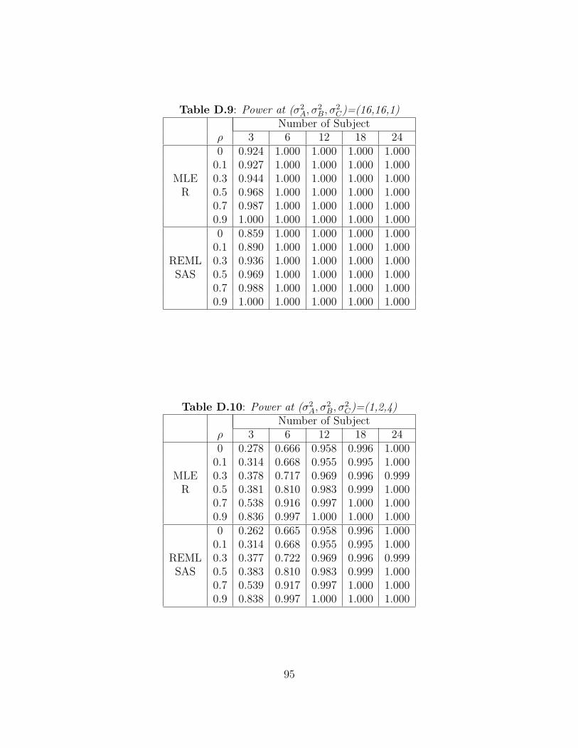
Table D.9: Power at (σ2A, σ
2B, σ
2C)=(16,16,1)
Number of Subjectρ 3 6 12 18 240 0.924 1.000 1.000 1.000 1.000
0.1 0.927 1.000 1.000 1.000 1.000MLE 0.3 0.944 1.000 1.000 1.000 1.000
R 0.5 0.968 1.000 1.000 1.000 1.0000.7 0.987 1.000 1.000 1.000 1.0000.9 1.000 1.000 1.000 1.000 1.0000 0.859 1.000 1.000 1.000 1.000
0.1 0.890 1.000 1.000 1.000 1.000REML 0.3 0.936 1.000 1.000 1.000 1.000SAS 0.5 0.969 1.000 1.000 1.000 1.000
0.7 0.988 1.000 1.000 1.000 1.0000.9 1.000 1.000 1.000 1.000 1.000
Table D.10: Power at (σ2A, σ
2B, σ
2C)=(1,2,4)
Number of Subjectρ 3 6 12 18 240 0.278 0.666 0.958 0.996 1.000
0.1 0.314 0.668 0.955 0.995 1.000MLE 0.3 0.378 0.717 0.969 0.996 0.999
R 0.5 0.381 0.810 0.983 0.999 1.0000.7 0.538 0.916 0.997 1.000 1.0000.9 0.836 0.997 1.000 1.000 1.0000 0.262 0.665 0.958 0.996 1.000
0.1 0.314 0.668 0.955 0.995 1.000REML 0.3 0.377 0.722 0.969 0.996 0.999SAS 0.5 0.383 0.810 0.983 0.999 1.000
0.7 0.539 0.917 0.997 1.000 1.0000.9 0.838 0.997 1.000 1.000 1.000
95
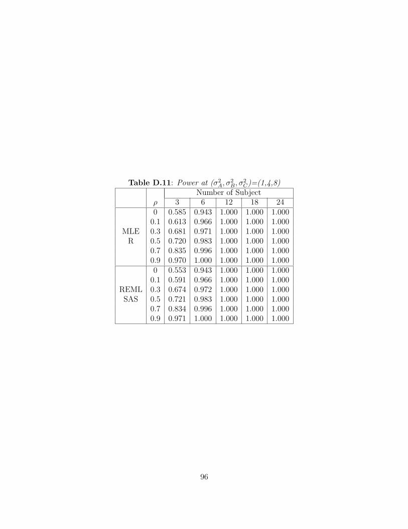
Table D.11: Power at (σ2A, σ
2B, σ
2C)=(1,4,8)
Number of Subjectρ 3 6 12 18 240 0.585 0.943 1.000 1.000 1.000
0.1 0.613 0.966 1.000 1.000 1.000MLE 0.3 0.681 0.971 1.000 1.000 1.000
R 0.5 0.720 0.983 1.000 1.000 1.0000.7 0.835 0.996 1.000 1.000 1.0000.9 0.970 1.000 1.000 1.000 1.0000 0.553 0.943 1.000 1.000 1.000
0.1 0.591 0.966 1.000 1.000 1.000REML 0.3 0.674 0.972 1.000 1.000 1.000SAS 0.5 0.721 0.983 1.000 1.000 1.000
0.7 0.834 0.996 1.000 1.000 1.0000.9 0.971 1.000 1.000 1.000 1.000
96
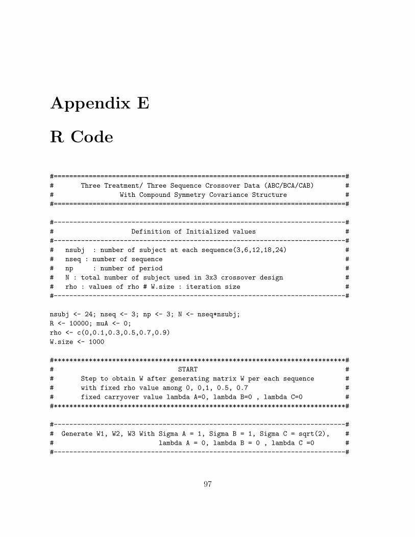
Appendix E
R Code
#===========================================================================## Three Treatment/ Three Sequence Crossover Data (ABC/BCA/CAB) ## With Compound Symmetry Covariance Structure ##===========================================================================#
#---------------------------------------------------------------------------## Definition of Initialized values ##---------------------------------------------------------------------------## nsubj : number of subject at each sequence(3,6,12,18,24) ## nseq : number of sequence ## np : number of period ## N : total number of subject used in 3x3 crossover design ## rho : values of rho # W.size : iteration size ##---------------------------------------------------------------------------#
nsubj <- 24; nseq <- 3; np <- 3; N <- nseq*nsubj;R <- 10000; muA <- 0;rho <- c(0,0.1,0.3,0.5,0.7,0.9)W.size <- 1000
#***************************************************************************## START ## Step to obtain W after generating matrix W per each sequence ## with fixed rho value among 0, 0,1, 0.5, 0.7 ## fixed carryover value lambda A=0, lambda B=0 , lambda C=0 ##***************************************************************************#
#---------------------------------------------------------------------------## Generate W1, W2, W3 With Sigma A = 1, Sigma B = 1, Sigma C = sqrt(2), ## lambda A = 0, lambda B = 0 , lambda C =0 ##---------------------------------------------------------------------------#
97
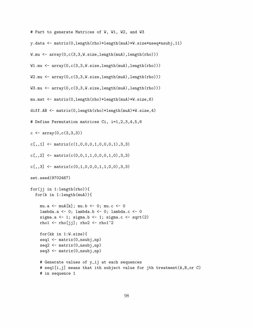
# Part to generate Matrices of W, W1, W2, and W3
y.data <- matrix(0,length(rho)*length(muA)*W.size*nseq*nsubj,11)
W.mu <- array(0,c(3,3,W.size,length(muA),length(rho)))
W1.mu <- array(0,c(3,3,W.size,length(muA),length(rho)))
W2.mu <- array(0,c(3,3,W.size,length(muA),length(rho)))
W3.mu <- array(0,c(3,3,W.size,length(muA),length(rho)))
mu.mat <- matrix(0,length(rho)*length(muA)*W.size,6)
diff.AB <- matrix(0,length(rho)*length(muA)*W.size,4)
# Define Permutation matrices Ci, i=1,2,3,4,5,6
c <- array(0,c(3,3,3))
c[,,1] <- matrix(c(1,0,0,0,1,0,0,0,1),3,3)
c[,,2] <- matrix(c(0,0,1,1,0,0,0,1,0),3,3)
c[,,3] <- matrix(c(0,1,0,0,0,1,1,0,0),3,3)
set.seed(9702467)
for(jj in 1:length(rho)){for(k in 1:length(muA)){
mu.a <- muA[k]; mu.b <- 0; mu.c <- 0lambda.a <- 0; lambda.b <- 0; lambda.c <- 0sigma.a <- 1; sigma.b <- 1; sigma.c <- sqrt(2)rho1 <- rho[jj]; rho2 <- rho1^2
for(kk in 1:W.size){seq1 <- matrix(0,nsubj,np)seq2 <- matrix(0,nsubj,np)seq3 <- matrix(0,nsubj,np)
# Generate values of y_ij at each sequences# seq1[i,j] means that ith subject value for jth treatment(A,B,or C)# in sequence 1
98

for(i in 1:nseq){for(j in 1:nsubj){
x1 <- rnorm(1,mean=0,sd=1)x2 <- rnorm(1,mean=0,sd=1)x3 <- rnorm(1,mean=0,sd=1)
# Sequence ABCif (i==1){
seq1[j,1]<-sigma.a*x1+mu.aseq1[j,2]<-rho1*sigma.b*x1+sigma.b*sqrt(1-rho2)*x2+mu.b+lambda.aseq1[j,3]<-rho1*sigma.c*x1+rho1*sigma.c*sqrt((1-rho1)/(1+rho1))*x2+
sigma.c*sqrt((1+rho1-2*rho2)/(1+rho1))*x3+mu.c+lambda.b
y.data[(jj-1)*length(muA)*W.size*nseq*nsubj+(k-1)*W.size*nseq*nsubj+(kk-1)*nseq*nsubj+(i-1)*nsubj+j,] <- c(rho[jj],sigma.a^2,sigma.b^2,sigma.c^2,nsubj,kk,i,j,seq1[j,1],seq1[j,2],seq1[j,3])
}# Sequence BCAif (i==2){
seq2[j,1]<-sigma.b*x1+mu.bseq2[j,2]<-rho1*sigma.c*x1+sigma.c*sqrt(1-rho2)*x2+mu.c+lambda.bseq2[j,3]<-rho1*sigma.a*x1+rho1*sigma.a*sqrt((1-rho1)/(1+rho1))*x2+
sigma.a*sqrt((1+rho1-2*rho2)/(1+rho1))*x3+mu.a+lambda.c
y.data[(jj-1)*length(muA)*W.size*nseq*nsubj+(k-1)*W.size*nseq*nsubj+(kk-1)*nseq*nsubj+(i-1)*nsubj+j,] <- c(rho[jj],sigma.a^2,sigma.b^2,sigma.c^2,nsubj,kk,i,j,seq2[j,1],seq2[j,2],seq2[j,3])
}# Sequence CABif (i==3){
seq3[j,1]<-sigma.c*x1+mu.cseq3[j,2]<-rho1*sigma.a*x1+sigma.a*sqrt(1-rho2)*x2+mu.a+lambda.cseq3[j,3]<-rho1*sigma.b*x1+rho1*sigma.b*sqrt((1-rho1)/(1+rho1))*x2+
sigma.b*sqrt((1+rho1-2*rho2)/(1+rho1))*x3+mu.b+lambda.a
y.data[(jj-1)*length(muA)*W.size*nseq*nsubj+(k-1)*W.size*nseq*nsubj+(kk-1)*nseq*nsubj+(i-1)*nsubj+j,] <- c(rho[jj],sigma.a^2,sigma.b^2,sigma.c^2,nsubj,kk,i,j,seq3[j,1],seq3[j,2],seq3[j,3])
}}
}
99
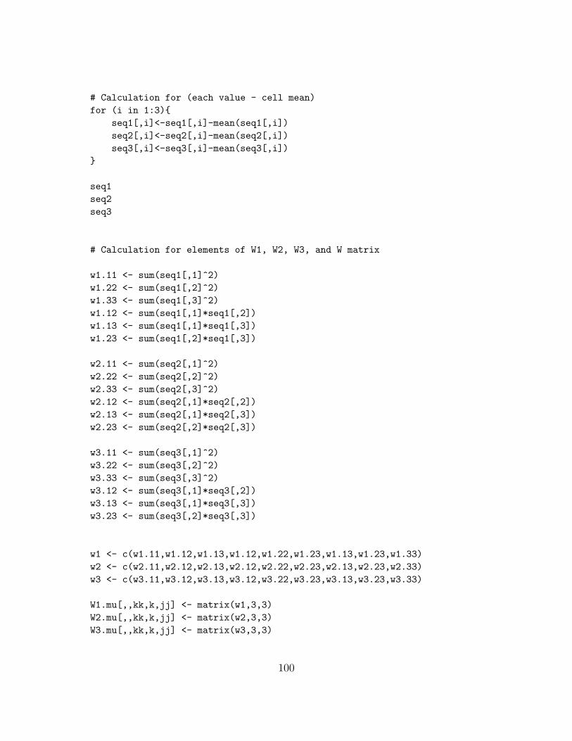
# Calculation for (each value - cell mean)for (i in 1:3){
seq1[,i]<-seq1[,i]-mean(seq1[,i])seq2[,i]<-seq2[,i]-mean(seq2[,i])seq3[,i]<-seq3[,i]-mean(seq3[,i])
}
seq1seq2seq3
# Calculation for elements of W1, W2, W3, and W matrix
w1.11 <- sum(seq1[,1]^2)w1.22 <- sum(seq1[,2]^2)w1.33 <- sum(seq1[,3]^2)w1.12 <- sum(seq1[,1]*seq1[,2])w1.13 <- sum(seq1[,1]*seq1[,3])w1.23 <- sum(seq1[,2]*seq1[,3])
w2.11 <- sum(seq2[,1]^2)w2.22 <- sum(seq2[,2]^2)w2.33 <- sum(seq2[,3]^2)w2.12 <- sum(seq2[,1]*seq2[,2])w2.13 <- sum(seq2[,1]*seq2[,3])w2.23 <- sum(seq2[,2]*seq2[,3])
w3.11 <- sum(seq3[,1]^2)w3.22 <- sum(seq3[,2]^2)w3.33 <- sum(seq3[,3]^2)w3.12 <- sum(seq3[,1]*seq3[,2])w3.13 <- sum(seq3[,1]*seq3[,3])w3.23 <- sum(seq3[,2]*seq3[,3])
w1 <- c(w1.11,w1.12,w1.13,w1.12,w1.22,w1.23,w1.13,w1.23,w1.33)w2 <- c(w2.11,w2.12,w2.13,w2.12,w2.22,w2.23,w2.13,w2.23,w2.33)w3 <- c(w3.11,w3.12,w3.13,w3.12,w3.22,w3.23,w3.13,w3.23,w3.33)
W1.mu[,,kk,k,jj] <- matrix(w1,3,3)W2.mu[,,kk,k,jj] <- matrix(w2,3,3)W3.mu[,,kk,k,jj] <- matrix(w3,3,3)
100

# Case of 3 Sequences
temp.1 <- t(c[,,1])%*%W1.mu[,,kk,k,jj]%*%c[,,1]temp.2 <- t(c[,,2])%*%W2.mu[,,kk,k,jj]%*%c[,,2]temp.3 <- t(c[,,3])%*%W3.mu[,,kk,k,jj]%*%c[,,3]
W.mu[,,kk,k,jj] <- temp.1+temp.2+temp.3
}}
}
y.data <- data.frame(y.data)
colnames(y.data) <-c("rho","sigmaA^2","sigmaB^2","sigmaC^2","nsubj","Sim","Seq","subj","y1","y2","y3")
write.table(y.data, file = "y24-112data.txt", sep = " ", row.names =F,qmethod = "double",quote=FALSE)
W.mean <- array(0,c(3,3,length(muA),length(rho)))
for(i in 1:length(rho)){for(j in 1:length(muA)){
W.temp <- matrix(0,3,3)
for(k in 1:W.size){W.temp <- W.temp + W.mu[,,k,j,i]
}
W.mean[,,j,i] <- W.temp/W.size
}}
#********************************************************************************#
#********************************************************************************#
# #
# Part of parameter estimation to make Sigma matrix #
# #
#********************************************************************************#
#********************************************************************************#
101
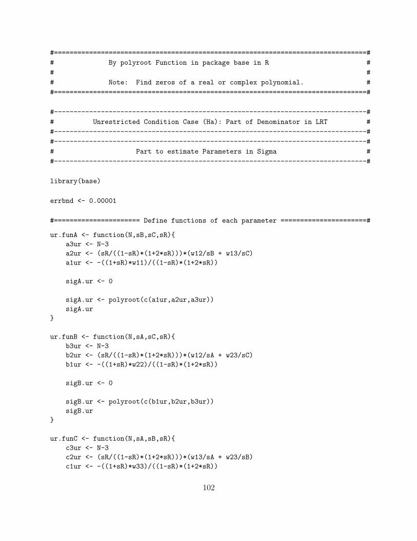
#================================================================================#
# By polyroot Function in package base in R #
# #
# Note: Find zeros of a real or complex polynomial. #
#================================================================================#
#--------------------------------------------------------------------------------#
# Unrestricted Condition Case (Ha): Part of Denominator in LRT #
#--------------------------------------------------------------------------------#
#--------------------------------------------------------------------------------#
# Part to estimate Parameters in Sigma #
#--------------------------------------------------------------------------------#
library(base)
errbnd <- 0.00001
#====================== Define functions of each parameter ======================#
ur.funA <- function(N,sB,sC,sR){a3ur <- N-3a2ur <- (sR/((1-sR)*(1+2*sR)))*(w12/sB + w13/sC)a1ur <- -((1+sR)*w11)/((1-sR)*(1+2*sR))
sigA.ur <- 0
sigA.ur <- polyroot(c(a1ur,a2ur,a3ur))sigA.ur
}
ur.funB <- function(N,sA,sC,sR){b3ur <- N-3b2ur <- (sR/((1-sR)*(1+2*sR)))*(w12/sA + w23/sC)b1ur <- -((1+sR)*w22)/((1-sR)*(1+2*sR))
sigB.ur <- 0
sigB.ur <- polyroot(c(b1ur,b2ur,b3ur))sigB.ur
}
ur.funC <- function(N,sA,sB,sR){c3ur <- N-3c2ur <- (sR/((1-sR)*(1+2*sR)))*(w13/sA + w23/sB)c1ur <- -((1+sR)*w33)/((1-sR)*(1+2*sR))
102

sigC.ur <- 0
sigC.ur <- polyroot(c(c1ur,c2ur,c3ur))sigC.ur
}
ur.funR <- function(N,sA0,sB0,sC0){
sA <- sA0; sB <- sB0; sC <- sC0
r4ur <- -6*(N-3)r3ur <- 3*(N-3) - (w11/sA^2 + w22/sB^2 + w33/sC^2)
+ 2*(w12/(sA*sB) + w13/(sA*sC) + w23/(sB*sC))r2ur <- 3*(N-3) - 2*(w11/sA^2 + w22/sB^2 + w33/sC^2)r1ur <- (w12/(sA*sB) + w13/(sA*sC) + w23/(sB*sC))
rho.ur <-0
temp1 <- Re(polyroot(c(r1ur,r2ur,r3ur,r4ur)))
if(abs(temp1[1]-temp1[2])< 0.0000000001) rho.ur <- temp1[3]if(abs(temp1[1]-temp1[3])< 0.0000000001) rho.ur <- temp1[2]if(abs(temp1[2]-temp1[3])< 0.0000000001) rho.ur <- temp1[1]
rho.ur}
logL <- function(N,c,W,sA0,sB0,sC0,sR0){
f <- log(c)+(N-7)*log(det(W))/2 -(N-3)/2*(log(sA0^2)+log(sB0^2)+log(sC0^2)+log((1+2*sR0)*(1-sR0)^2))-(1+sR0)/(2*(1-sR0)*(1+2*sR0))*(W[1,1]/sA0^2 +W[2,2]/sB0^2 +W[3,3]/sC0^2)+sR0/((1-sR0)*(1+2*sR0))*(W[1,2]/(sA0*sB0)+W[1,3]/(sA0*sC0)+W[2,3]/(sB0*sC0))
f}
#=============================== Procedure 2 ==============================#
ini.ur2 <- matrix(0,length(rho)*length(muA)*W.size,7)
est.ur2 <- matrix(0,length(rho)*length(muA)*W.size,7)
ini.val2 <- rep(0,7); err.val2 <- rep(0,7); logL.val2 <- rep(0,4)
103

Con2<-2^(3*(N-3)/2)*pi^(3/2)*gamma((N-3)/2)*gamma((N-4)/2)*gamma((N-5)/2)
# Start - FOR statement for rho for(i in 1:length(rho)){
# Start - FOR statement for muAfor(j in 1:length(muA)){
# Start - FOR statement for W.sizefor(k in 1:W.size){
w11 <- W.mu[1,1,k,j,i]; w22 <- W.mu[2,2,k,j,i]; w33 <- W.mu[3,3,k,j,i]w12 <- W.mu[1,2,k,j,i]; w13 <- W.mu[1,3,k,j,i]; w23 <- W.mu[2,3,k,j,i]
sA0 <- sqrt(w11/(N-3)); sB0 <- sqrt(w22/(N-3)); sC0 <- sqrt(w33/(N-3))sR0 <- (w12/sqrt(w11*w22) + w13/sqrt(w11*w33) + w23/sqrt(w22*w33))/3ini.ur2[(i-1)*length(muA)*W.size+(j-1)*W.size+k,]
<- c(rho[i],muA[j],k,sA0,sB0,sC0,sR0)
logL1 <- c(rho[i],muA[j],k,logL(N,1/Con2,W.mu[,,k,j,i],sA0,sB0,sC0,sR0))
sigA <- c(rho[i],muA[j],k,sA0)sigB <- c(rho[i],muA[j],k,sB0)sigC <- c(rho[i],muA[j],k,sC0)sigR <- c(rho[i],muA[j],k,sR0)
#err2.ur1 <- c(rho[i],muA[j],k,0)err2.ur1 <- c(rho[i],muA[j],k,0,0,0,0)ini2.ur1 <- c(rho[i],muA[j],k,sA0,sB0,sC0,sR0)
# Start - REPEAT statementrepeat{
sA1 <- Re(ur.funA(N,sB0,sC0,sR0))[1]sigA <- rbind(sigA,c(rho[i],muA[j],k,sA1))
sB1 <- Re(ur.funB(N,sA1,sC0,sR0))[1]sigB <- rbind(sigB,c(rho[i],muA[j],k,sB1))
sC1 <- Re(ur.funC(N,sA1,sB1,sR0))[1]sigC <- rbind(sigC,c(rho[i],muA[j],k,sC1))
sR1 <- ur.funR(N,sA1,sB1,sC1)sigR <- rbind(sigR,c(rho[i],muA[j],k,sR1))
104

logL0 <- c(rho[i],muA[j],k,logL(N,1/Con2,W.mu[,,k,j,i],sA1,sB1,sC1,sR1))logL1 <- rbind(logL1,logL0)
ini2.ur1 <- rbind(ini2.ur1,c(rho[i],muA[j],k,sA1,sB1,sC1,sR1))
e1 <- abs(sA1-sA0)e2 <- abs(sB1-sB0)e3 <- abs(sC1-sC0)e4 <- abs(sR1-sR0)
err2.ur0 <- c(rho[i],muA[j],k,e1,e2,e3,e4)err2.ur1 <- rbind(err2.ur1,err2.ur0)
# Start - IF statementif((e1 <= errbnd) && (e2 <= errbnd) && (e3 <= errbnd) && (e4 <= errbnd)){
est.ur2[(i-1)*length(muA)*W.size+(j-1)*W.size+k,]<- c(rho[i],muA[j],k,sA1,sB1,sC1,sR1)
break}# End - IF statement
sA0 <- sA1sB0 <- sB1sC0 <- sC1sR0 <- sR1}# End - REPEAT statement
ini.val2 <- rbind(ini.val2,ini2.ur1)err.val2 <- rbind(err.val2,err2.ur1)logL.val2 <- rbind(logL.val2,logL1)
}# End - FOR statement for W.size
}# End - FOR statement for muA
} # End - FOR statement for rho
est.ur2 <- data.frame(est.ur2)
colnames(est.ur2)<-c("rho","muA","Rep","Est-sigma A","Est-sigmaB","Est-sigma C","Est-rho")
105

est.ur2.mean <- matrix(0,length(rho)*length(muA),6)
for(i in 1:length(rho)){for(j in 1:length(muA)){t.4 <- est.ur2[(((i-1)*length(muA)*W.size+(j-1)*W.size+1):
((i-1)*length(muA)*W.size+(j-1)*W.size+W.size)),4]t.5 <- est.ur2[(((i-1)*length(muA)*W.size+(j-1)*W.size+1):
((i-1)*length(muA)*W.size+(j-1)*W.size+W.size)),5]t.6 <- est.ur2[(((i-1)*length(muA)*W.size+(j-1)*W.size+1):
((i-1)*length(muA)*W.size+(j-1)*W.size+W.size)),6]t.7 <- est.ur2[(((i-1)*length(muA)*W.size+(j-1)*W.size+1):
((i-1)*length(muA)*W.size+(j-1)*W.size+W.size)),7]
t1<-sqrt(sum(t.4^2)/W.size)t2<-sqrt(sum(t.5^2)/W.size)t3<-sqrt(sum(t.6^2)/W.size)t4<-mean(t.7)
est.ur2.mean[(i-1)*length(muA)+j,] <-c(Re(rho[i]),Re(muA[j]),Re(t1),Re(t2),Re(t3),Re(t4))
}}
est.ur2.mean <- data.frame(est.ur2.mean)
colnames(est.ur2.mean) <- c(" rho "," muA ","Est-Sigma A","Est-SigmaB","Est-Sigma C","Est-Rho")
#--------------------------------------------------------------------------------## Restricted Condition Case (H0): Part of Numerator in LRT ##--------------------------------------------------------------------------------##--------------------------------------------------------------------------------## Part to estimate Parameters in Sigma ##--------------------------------------------------------------------------------#
ini.r <- matrix(0,length(rho)*length(muA)*W.size,5)
sig.r <- matrix(0,length(muA)*length(rho)*W.size,4)
rho.r <- matrix(0,length(muA)*length(rho)*W.size,4)
106

temp.r <- matrix(0,length(muA)*length(rho)*W.size,3)
for(i in 1:length(rho)){for(j in 1:length(muA)){for(k in 1:W.size){
w11 <- W.mu[1,1,k,j,i]; w22 <- W.mu[2,2,k,j,i]; w33 <- W.mu[3,3,k,j,i]w12 <- W.mu[1,2,k,j,i]; w13 <- W.mu[1,3,k,j,i]; w23 <- W.mu[2,3,k,j,i]
# sA and sR are Shanga’s MLE of parameter sigma A and rho# under the restricted condition
sA <- (w11+w22+w33)/(3*(N-3))sR <- (w12+w13+w23)/(w11+w22+w33)ini.r[(i-1)*length(muA)*W.size+(j-1)*W.size+k,] <- c(rho[i],muA[j],k,sA,sR)
# We can get sigma^2 directly because there is no 1st order term
a3r <- 3*(N-3)a2r <- 0a1r <- ((1+sR)*(w11+w22+w33)-2*sR*(w12+w13+w23))/((1-sR)*(1+2*sR))
# We have to choose one real root from polyroot function
r4r <- -6*(N-3)r3r <- 3*(N-3) - (w11+w22+w33)/sA + 2*(w12+w13+w23)/sAr2r <- 3*(N-3) - 2*(w11+w22+w33)/sAr1r <- (w12+w13+w23)/sA
sig.r[(i-1)*length(muA)*W.size+(j-1)*W.size+k,] <- c(rho[i],muA[j],k,a1r/a3r)
temp.r[(i-1)*length(muA)*W.size+(j-1)*W.size+k,] <- Re(polyroot(c(r1r,r2r,r3r,r4r)))temp1 <- temp.r[(i-1)*length(muA)*W.size+(j-1)*W.size+k,]
if(abs(temp1[1]-temp1[2])< 0.0000000001){rho.r[(i-1)*length(muA)*W.size+(j-1)*W.size+k,] <- c(rho[i],muA[j],k,temp1[3])}
if(abs(temp1[2]-temp1[3])< 0.0000000001){rho.r[(i-1)*length(muA)*W.size+(j-1)*W.size+k,] <- c(rho[i],muA[j],k,temp1[1])}
if(abs(temp1[1]-temp1[3])< 0.0000000001){rho.r[(i-1)*length(muA)*W.size+(j-1)*W.size+k,] <- c(rho[i],muA[j],k,temp1[2])}
}}
}
107

sig.r <- data.frame(sig.r)
colnames(sig.r) <- c("rho","muA","Rep","Est-SigSq")
rho.r <- data.frame(rho.r)
colnames(rho.r) <- c("rho","muA","Rep","Est-rho")
est.r <- cbind(abs(sig.r[,1:3]),Re(sig.r[,4]),Re(rho.r[,4]))
est.r <- data.frame(est.r)
colnames(est.r) <- c("rho","muA","Rep","Est-SigSq","Est-rho")
est.r2.mean <- matrix(0,length(rho)*length(muA),4)
for(i in 1:length(rho)){for(j in 1:length(muA)){
t1<-sqrt(sum(est.r[(((i-1)*length(muA)*W.size+(j-1)*W.size+1):((i-1)*length(muA)*W.size+(j-1)*W.size+W.size)),4])/W.size)
t2<-mean(est.r[(((i-1)*length(muA)*W.size+(j-1)*W.size+1):((i-1)*length(muA)*W.size+(j-1)*W.size+W.size)),5])
est.r2.mean[(i-1)*length(muA)+j,] <- c(Re(rho[i]),Re(muA[j]),Re(t1),Re(t2))
}}
est.r2.mean <- data.frame(est.r2.mean)
colnames(est.r2.mean) <- c(" rho "," muA ","Est-Sigma^2","Est-Rho")
#=============================================================================## LIKELIHOOD RATIO TEST ##=============================================================================##-----------------------------------------------------------------------------## New: Likelihood Ratio Test with MLEs of parameter Sigma-A,-B,-C, and rho ##-----------------------------------------------------------------------------#
# Part to compute Determinant of W1, W2, W3, and W
W0.det <- rep(0,length(rho)*length(muA)*W.size)
108

for(i in 1:length(rho)){for(j in 1:length(muA)){for(k in 1:W.size){
W0.det[(i-1)*length(muA)*W.size+(j-1)*W.size+k] <- det(W.mu[,,k,j,i])
}}
}
W0.det
# Under Ha(Unrestricted condition): sigh1.mat, sigh2.mat, sigh3.mat# Under H0(Restricted condition): sigh.mat
sigha.mat <- array(0,c(3,3,W.size,length(muA),length(rho)))sigh0.mat <- array(0,c(3,3,W.size,length(muA),length(rho)))
for(i in 1:length(rho)){for(j in 1:length(muA)){for(k in 1:W.size){
e11 <- est.ur2[(i-1)*length(muA)*W.size+(j-1)*W.size+k,4]e22 <- est.ur2[(i-1)*length(muA)*W.size+(j-1)*W.size+k,5]e33 <- est.ur2[(i-1)*length(muA)*W.size+(j-1)*W.size+k,6]r <- est.ur2[(i-1)*length(muA)*W.size+(j-1)*W.size+k,7]
e0 <- est.r[(i-1)*length(muA)*W.size+(j-1)*W.size+k,4]r0 <- est.r[(i-1)*length(muA)*W.size+(j-1)*W.size+k,5]
d.a <- c(e11,0,0,0,e22,0,0,0,e33)d.0 <- c(sqrt(e0),0,0,0,sqrt(e0),0,0,0,sqrt(e0))
w.a <- c(1,r,r,r,1,r,r,r,1)w.0 <- c(1,r0,r0,r0,1,r0,r0,r0,1)
sigha.mat[,,k,j,i] <- matrix(d.a,3,3)%*% matrix(w.a,3,3)%*%matrix(d.a,3,3)sigh0.mat[,,k,j,i] <- matrix(d.0,3,3)%*%matrix(w.0,3,3)%*%matrix(d.0,3,3)
}}
}
109

sigha.matsigh0.mat
# Part to compute Determinant of sigma_1_hat, sigma_2_hat,# sigma_3_hat, and sigma_hat
Sh0.det <- rep(0,length(rho)*length(muA)*W.size)
Sha.det <- rep(0,length(rho)*length(muA)*W.size)
for(i in 1:length(rho)){for(j in 1:length(muA)){for(k in 1:W.size){
Sh0.det[(i-1)*length(muA)*W.size+(j-1)*W.size+k] <- det(sigh0.mat[,,k,j,i])Sha.det[(i-1)*length(muA)*W.size+(j-1)*W.size+k] <- det(sigha.mat[,,k,j,i])
}}
}
Sh0.detSha.det
# Part to compute Inverse Matrix of sigma_1_hat, sigma_2_hat,# sigma_3_hat, and sigma_hat# Here used Generalized Inverse from MASS Library
library(MASS)
Sh0.inv <- array(0,c(3,3,W.size,length(muA),length(rho)))
Sha.inv <- array(0,c(3,3,W.size,length(muA),length(rho)))
for(i in 1:length(rho)){for(j in 1:length(muA)){for(k in 1:W.size){
Sh0.inv[,,k,j,i] <- ginv(sigh0.mat[,,k,j,i])Sha.inv[,,k,j,i] <- ginv(sigha.mat[,,k,j,i])
}}
}
110

Sh0.inv Sha.inv
# Part to compute tr(W*sigma_hat_inverse) under H0# Part to compute tr(W*sigma1_hat_inverse),tr(W*sigma2_hat_inverse)# and tr(W*sigma3_hat_inverse) under Ha
tr.0 <- rep(0,length(rho)*length(muA)*W.size)
tr.a <- rep(0,length(rho)*length(muA)*W.size)
for(i in 1:length(rho)){for(j in 1:length(muA)){for(k in 1:W.size){
tr.0[(i-1)*length(muA)*W.size+(j-1)*W.size+k]<- sum(diag(W.mu[,,k,j,i]%*%Sh0.inv[,,k,j,i]))
tr.a[(i-1)*length(muA)*W.size+(j-1)*W.size+k] <-<- sum(diag(W.mu[,,k,j,i]%*%Sha.inv[,,k,j,i]))
}}
}
tr.0tr.a
# Part to compute the value of Gamma function multiplication# under H0 and Ha
gam.1 <- gamma((3*nsubj-3)/2)
gam.2 <- gamma((3*nsubj-4)/2)
gam.3 <- gamma((3*nsubj-5)/2)
gam.1;gam.2;gam.3
# Part to construct lambda function to test H0 vs Ha
lam.num <- rep(0,length(rho)*length(muA)*W.size)
lam.den <- rep(0,length(rho)*length(muA)*W.size)
111

LRT.lambda <- rep(0,length(rho)*length(muA)*W.size)
Q.nLRT <- matrix(0,length(muA)*W.size,length(rho))
lam.num <- rep(0,length(rho)*length(muA)*W.size)
rej.nLRT <- matrix(0,length(rho)*length(muA),4)
for(i in 1:length(rho)){for(j in 1:length(muA)){cnt <- 0for(k in 1:W.size){
# Part to compute the numerator part of lambda
part1.num <- W0.det[(i-1)*length(muA)*W.size+(j-1)*W.size+k]^((3*nsubj-7)/2)*exp(-tr.0[(i-1)*length(muA)*W.size+(j-1)*W.size+k]/2)
part2.num <- Sh0.det[(i-1)*length(muA)*W.size+(j-1)*W.size+k]^((3*(nsubj-1))/2)
lam.num[(i-1)*length(muA)*W.size+(j-1)*W.size+k] <- part1.num/(part2.num*(gam.1*gam.2*gam.3)*(2^((3*(3*nsubj-3))/2))*(pi^((np*(np-1))/4)))
l.num <- lam.num[(i-1)*length(muA)*W.size+(j-1)*W.size+k]
# Part to compute the denominator part of lambda
part1.den <- W0.det[(i-1)*length(muA)*W.size+(j-1)*W.size+k]^((3*nsubj-7)/2)*exp(-tr.a[(i-1)*length(muA)*W.size+(j-1)*W.size+k]/2)
part2.den <- Sha.det[(i-1)*length(muA)*W.size+(j-1)*W.size+k]^((3*(nsubj-1))/2)
lam.den[(i-1)*length(muA)*W.size+(j-1)*W.size+k] <- part1.den/(part2.den*(gam.1*gam.2*gam.3)*(2^((3*(3*nsubj-3))/2))*(pi^((np*(np-1))/4)))
l.den <- lam.den[(i-1)*length(muA)*W.size+(j-1)*W.size+k]
LRT.lambda[(i-1)*length(muA)*W.size+(j-1)*W.size+k] <- l.num/l.den
Q.nLRT[(j-1)*W.size+k,i] <- -2*log(LRT.lambda[(i-1)*length(muA)*W.size+(j-1)*W.size+k])
if(Q.nLRT[(j-1)*W.size+k,i] > qchisq(1-0.05,df=2, ncp=0, log = FALSE))cnt <- cnt+1
}
rej.nLRT[(i-1)*length(muA)+j,] <- c(rho[i],muA[j],cnt,cnt/W.size)
112

}}
lam.numlam.denLRT.lambdaQ.nLRT
rej.nLRT <- data.frame(rej.nLRT)
colnames(rej.nLRT) <- c(" rho "," muA ","# Rej/1000"," Ratio ")
est.r2.meanest.ur2.meanrej.nLRT
113
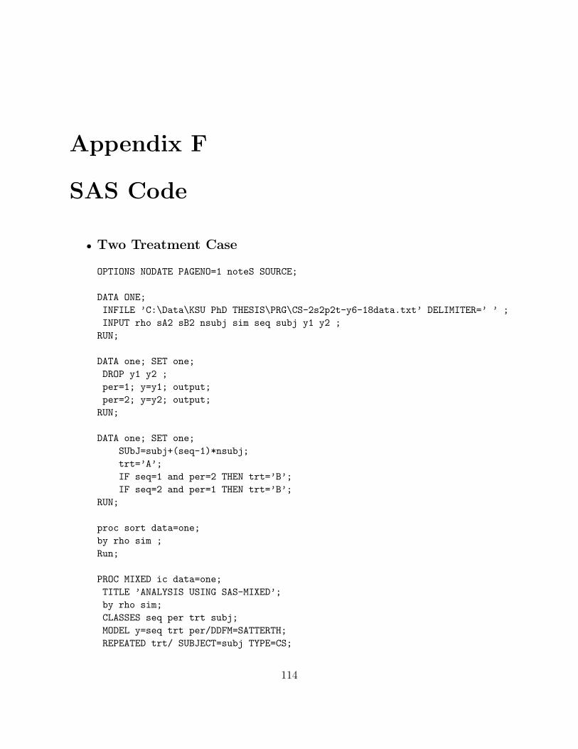
Appendix F
SAS Code
• Two Treatment Case
OPTIONS NODATE PAGENO=1 noteS SOURCE;
DATA ONE;INFILE ’C:\Data\KSU PhD THESIS\PRG\CS-2s2p2t-y6-18data.txt’ DELIMITER=’ ’ ;INPUT rho sA2 sB2 nsubj sim seq subj y1 y2 ;RUN;
DATA one; SET one;DROP y1 y2 ;per=1; y=y1; output;per=2; y=y2; output;RUN;
DATA one; SET one;SUbJ=subj+(seq-1)*nsubj;trt=’A’;IF seq=1 and per=2 THEN trt=’B’;IF seq=2 and per=1 THEN trt=’B’;
RUN;
proc sort data=one;by rho sim ;Run;
PROC MIXED ic data=one;TITLE ’ANALYSIS USING SAS-MIXED’;by rho sim;CLASSES seq per trt subj;MODEL y=seq trt per/DDFM=SATTERTH;REPEATED trt/ SUBJECT=subj TYPE=CS;
114

ods listing exclude all;ods output infocrit = null COVPARMS=HOPARMS;RUN;
PROC SORT DATA=HOPARMS;BY RHO COVPARM;
PROC MEANS;BY RHO COVPARM;RUN;
DATA null; set null;rename neg2loglike =ho;drop aic--caic;
PROC MIXED ic data = one;TITLE ’ANALYSIS USING SAS-MIXED’;by rho sim;CLASSES seq per trt subj;MODEL y=seq trt per/DDFM=SATTERTH;REPEATED trt/ SUBJECT=subj TYPE=CSH;ods listing exclude all;ods output infocrit=ha COVPARMS=HAPARMS;RUN;
PROC SORT DATA=HAPARMS;BY RHO COVPARM;
PROC MEANS;BY RHO COVPARM;RUN;
DATA ha; SET ha;rename neg2loglike =ha;drop aic--caic;
DATA comb;merge null ha;by rho sim;RUN;
DATA comb;SET comb;u = ho-ha;IF u>3.841459 THEN reject=1; ELSE reject=0;
115

RUN;
PROC MEANS data=comb; by rho;ods listing select all;var reject;RUN;
QUIT;
• Three Treatment Case
OPTIONS NODATE PAGENO=1 noteS SOURCE;
DATA ONE;INFILE ’C:\Data\KSU PhD THESIS\PRG\y12-148data.txt’ DELIMITER=’ ’;INPUT rho sA2 sB2 sC2 nsubj sim seq subj y1 y2 y3;RUN;
DATA one; SET one;DROP y1 y2 y3;per=1; y=y1; output;per=2; y=y2; output;per=3; y=y3; output;RUN;
DATA one; SET one;SUbJ=subj+(seq-1)*nsubj;trt=’A’;IF seq=1 and per=2 THEN trt=’B’;IF seq=1 and per=3 THEN trt=’C’;
IF seq=2 and per=1 THEN trt=’B’;IF seq=2 and per=2 THEN trt=’C’;
IF seq=3 and per=1 THEN trt=’C’;IF seq=3 and per=3 THEN trt=’B’;
RUN;
proc sort data=one;by rho sim ;Run;
PROC MIXED ic data=one;TITLE ’ANALYSIS USING SAS-MIXED’;by rho sim;CLASSES seq per trt subj;
116

MODEL y=seq trt per/DDFM=SATTERTH;REPEATED trt/ SUBJECT=subj TYPE=CS;ods listing exclude all;ods output infocrit = null COVPARMS=HOPARMS;RUN;
PROC SORT DATA=HOPARMS;BY RHO COVPARM;
PROC MEANS;BY RHO COVPARM;RUN;
DATA null; set null;rename neg2loglike =ho;drop aic--caic;
PROC MIXED ic data = one;TITLE ’ANALYSIS USING SAS-MIXED’;by rho sim;CLASSES seq per trt subj;MODEL y=seq trt per/DDFM=SATTERTH;REPEATED trt/ SUBJECT=subj TYPE=CSh;ods listing exclude all;ods output infocrit=ha COVPARMS=HAPARMS;RUN;
PROC SORT DATA=HAPARMS;BY RHO COVPARM;
PROC MEANS;BY RHO COVPARM;RUN;
DATA ha; set ha;rename neg2loglike =ha;drop aic--caic;
DATA comb;merge null ha;by rho sim;RUN;
DATA comb;SET comb;
117

u = ho-ha;IF u>5.991465 THEN reject=1; ELSE reject=0;RUN;
PROC MEANS data=comb;by rho;ods listing select all;var reject;RUN;
QUIT;
118


![BeST - Bioequivalence Study Templatestudy carried out to evaluate the bioequivalence of two medicinal products. The bioequivalence studies are strictly regulated [1] and are therefore](https://img.pdfslide.us/doc/110x75/5ed9f97c28db2d5ca2492e81/best-bioequivalence-study-template-study-carried-out-to-evaluate-the-bioequivalence.jpg)