Guard Automata for the Verification of Safety and Liveness

HAL Id: hal-03283388https://hal.inria.fr/hal-03283388

Submitted on 10 Jul 2021

HAL is a multi-disciplinary open accessarchive for the deposit and dissemination of sci-entific research documents, whether they are pub-lished or not. The documents may come fromteaching and research institutions in France orabroad, or from public or private research centers.

L’archive ouverte pluridisciplinaire HAL, estdestinée au dépôt et à la diffusion de documentsscientifiques de niveau recherche, publiés ou non,émanant des établissements d’enseignement et derecherche français ou étrangers, des laboratoirespublics ou privés.

Guard Automata for the Verification of Safety andLiveness of Distributed Algorithms (long version)

Nathalie Bertrand, Bastien Thomas, Josef Widder

To cite this version:Nathalie Bertrand, Bastien Thomas, Josef Widder. Guard Automata for the Verification of Safetyand Liveness of Distributed Algorithms (long version). [Technical Report] Inria. 2021, pp.1-33. �hal-03283388�

https://hal.inria.fr/hal-03283388

https://hal.archives-ouvertes.fr

Guard Automata for the Verification of Safety andLiveness of Distributed Algorithms (long version)Nathalie Bertrand !

Univ Rennes, Inria, CNRS, IRISA, France

Bastien Thomas !

Univ Rennes, Inria, CNRS, IRISA, France

Josef Widder !

Informal Systems, Austria

AbstractDistributed algorithms typically run over arbitrary many processes and may involve unboundedlymany rounds, making the automated verification of their correctness challenging. Building on domaintheory, we introduce a framework that abstracts infinite-state distributed systems that representdistributed algorithms into finite-state guard automata. The soundness of the approach correspondsto the Scott-continuity of the abstraction, which relies on the assumption that the distributedalgorithms are layered. Guard automata thus enable the verification of safety and liveness propertiesof distributed algorithms.

2012 ACM Subject Classification Theory of computation → Verification by model checking; Theoryof computation → Distributed algorithms

Keywords and phrases Verification, Distributed algorithms, Domain theory

Acknowledgements This project has received funding from Interchain Foundation (Switzerland).

1 Introduction

Under the umbrella of parameterized verification, the verification of systems formed of anarbitrary number of agents executing the same code, has attracted quite some attentionin the recent years, see for instance [18, 9]. Application examples range from distributedalgorithms (e.g., for clock synchronization [28] or robot coordination [27]), cache-coherenceprotocols [25, 1], to chemical or biological systems [10]. In all cases, the systems are designedto operate correctly independently of the number of agents.

More specifically, distributed algorithms are central to various emblematic applications,including telecommunications, scientific computing, and Blockchain. Automatically provingthe correctness of distributed algorithms is a particularly relevant, as stated by Lamport:“Model-checking algorithms prior to submitting them for publication should become thenorm” [22]. The task, that the verification community has started to address, is quitechallenging, since it aims at validating at once all instances of the algorithm for arbitrarilymany processes.

Distributed algorithms with threshold guards are omni-present in solutions for consensusand agreement problems. Typically, these guards also are parameterized, e.g., if the numberof processes in a distributed system is n, then it is natural to require that certain actionsare taken only if a majority of processes is ready to do so; this results in a parameterizedthreshold expression of n/2. Due to Blockchain and other current applications these kinds ofdistributed algorithm enjoy recent attention from the algorithm design community as well asthe verification community. the algorithm design community has been studying them for along time, (see e.g., [11]) and typically provides hand-written proofs based on mathematicalmodels without formal semantics.

mailto:[email protected]

http://orcid.org/0000-0002-9957-5394



2 Guard Automata for the Verification of Distributed Algorithms (long version)

For computer-aided verification the first challenge is to develop appropriate modelingformalisms that maintain all behaviors of the original algorithms on the one hand, and onthe other hand are abstract and succinct to allow for efficient verification. Several approachestowards efficient verification have recently been proposed.

The threshold automata framework [20] targets asynchronous distributed algorithmswith threshold guards and reductions (similar to [23, 17]) have been used to show thatSMT-based bounded model checking is complete [19]. Later this framework was generalizedand generalizations were analyzed regarding decidability [21], and complexity [5]. The currentpaper also targets threshold distributed algorithms, yet eventually provides an even coarserabstraction to represent their behaviors, thus reducing the overall verification complexity.Moreover, the semantics of distributed algorithms and the soundness of the abstraction relyon domain theory concepts, thus providing a solid mathematical framework to our work.Last but not least, our approach can handle infinite behaviours, in contrast to the thresholdautomata framework.

The logical fragment of the IVy toolset has also been shown to allow to model thresholdguards by axiomising their semantics as quorum systems [7]. For instance, the reasonfor waiting for quorums of more than n/2 messages is that any two such quorums mustintersect at one sender. IVy allows to express these quorum axioms and reduce verificationto decidable fragments. Similar intuitions underlie verification results in the heard-of model(HO model) [13]. This computational model for distributed algorithms already targets a highlevel of abstractions that are sound for communication closed distributed algorithms [12].Here a consensus logic was introduced in [16] that could be used for deductive verificationand cut-off results where provided in [24] that reduce the parameterized verification problemto small finite instances. Compared to this line of work, the distributed algorithms we targetshare some similarities with these round-based communication closed models. Recently, athreshold automata framework for round-based algorithms was introduced that also uses asmall counterexample property for verification in [29]. In contrast, we use domain theory, andparticularly Scott continuity to be able to reason on infinite behaviors and thus to capturealgorithms that do not necessarily terminate.

Other less related verification frameworks also target distributed algorithms with quitedifferent techniques such as event B [26], array systems [4] or logic and automata theory [3].

Contributions

Using basic domain theory concepts, we provide a rigorous framework to model and verify(asynchronous) distributed algorithms. Our methodology applies to distributed algorithmsthat are structured in layers (that can be seen as a fine-grain notion of rounds), and mayconsist of countably many layers, thus capturing round-based distributed algorithms (withno a priori bound on the number of rounds).

In Section 2, we define partially ordered transition systems, which serve to express thesemantics our models.Section 3 introduces the low-level model of layered distributed systems to representthreshold based distributed algorithms. The state-space of layered distributed systemsbeing infinite (and even not necessarily finitely representable), we provide several abstrac-tion steps, up to a so-called guard abstraction. The soundness of each step is justified bythe Scott-continuity of the corresponding abstraction. Some steps are also complete, andthus do not introduce spurious behaviors.Finally, towards practical verification, we define in Section 4 the guard automaton, afinite-state abstraction of (cyclic) layered distributed systems. It overapproximates the

N. Bertrand, B. Thomas and J. Widder 3

set of infinite behaviors of distributed algorithms, and thus enabling the verification ofsafety as well as liveness properties. Its construction can be automated with the help ofan SMT solver, paving the way to the automated verification of round-based thresholddistributed algorithms.

2 A Fistful of Domain Theory

2.1 Mathematical PreliminariesThis section presents mathematical notions as well as notations that are used throughout thepaper. In particular, it introduces partially ordered sets and Scott topology. The interestedreader is referred to [2] for an thorough introduction to domain theory.

Sets and multisets. A multiset over a set X is an element of NX . Addition andinclusion over multisets are defined in a natural way. For ξ, ξ′ ∈NX two multisets, ξ+ξ′ ∈NX

is the multiset such that for every x ∈ X, (ξ + ξ′) (x) = ξ(x) + ξ′(x). We write ξ ⊑ ξ′ if forevery x ∈X, ξ(x) ≤ ξ′(x). Standard sets can be seen as special cases of multisets with thecanonical bijection between the set of subsets of X (2X) and the set of functions from X to{0,1}.

Sequences. For X a set and n ∈ N a natural number, a sequence of elements of X oflength n is some u ∈X{0,...,n−1}. Its length is ∣u∣ = n and for i < n, u(i) ∈X denotes the letterat index i. X∗ = ⋃n∈NX

{0,...,n−1} (resp. X+ = ⋃n>0X{0,...,n−1}) denotes the set of all finite

(resp. finite and non-empty) sequences of elements of X. Moreover, X∗ = X∗ ∪XN is theset of finite or infinite sequences of X. For u ∈ X∗ a finite sequence and v ∈ X∗ a finite orinfinite sequence, we write u ⋅ v for the concatenation of u and v. For u and w two sequences,we write u ≺ w and say that u is a prefix of w if either w is finite and there exists v ∈ X∗such that u ⋅ v = w or u = w. For w a sequence and i ≤ ∣w∣, wi is the prefix w of length i.

Closures and bounds for partially ordered sets. Let (X,⊑) be a partially orderedset, and ξ ⊂X. The upward-closure of ξ is ↑ξ = {x ∈X ∣ ∃x′ ∈ ξ, x′ ⊑ x}, and ξ is upward-closedif ↑ξ = ξ. Dually, one defines the downward-closure ↓ξ and downward-closed sets. An elementx ∈X is an upper-bound of ξ if for any element x′ ∈ ξ, x′ ⊑ x. We write ub(ξ) for the set ofupper-bounds of ξ. If it exists (it is then unique), the greatest element of ξ is x ∈ X suchthat x ∈ ξ and x ∈ ub(ξ). Dually, one defines the notion of least element by reversing theorder. If it exists, the least upper bound of ξ is the least element of ub(ξ), and we denoteit by ⊔ ξ. Finally ξ is directed if it is non-empty and if for every two elements x,x′ ∈ ξ,ub({x,x′})∩ ξ ≠ ∅; intuitively, any finite subset of ξ has an upper-bound in ξ. An interestingparticular case of directed case are completely ordered sets which are called chains in thiscontext.

Directed Complete Partially ordered sets (DCPO). A DCPO is a partially orderedset (X,⊑) such that any directed subset ξ ⊂ X has a (unique) least upper bound. Thesepartially ordered sets are particularly important in semantics of programming languages.

The Scott Topology on DCPO. Directed complete partial orders are naturallyequipped with the Scott topology. A subset ξ of a DCPO (X,⊑) is Scott-closed if it isdownward-closed and if for any directed subset ξ′ ⊂ ξ, ⊔ ξ′ ∈ ξ. A subset is Scott-open if itscomplement in X is Scott-closed. Functions that are continuous for the Scott topology arecalled Scott-continuous. A function f ∶ X → Y is monotonous if for any x,x′ ∈ X, if x ⊑ x′then f(x) ⊑ f(x′). A Scott-continuous function is always monotonous. A function f ∶X → Y

is Scott-continuous if and only if for any directed subset ξ ⊂ X, f(⊔(ξ)) = ⊔(f(ξ)). Inthis paper, a partial function f ∶ X → Y is called Scott-continuous if its domain dom(f) isScott-closed and if for any directed subset ξ ⊂ dom(f), f(⊔ ξ) = ⊔ f(ξ).


2.2 Partially Ordered Transition SystemsBuilding on domain theory, this section introduces a generic model for distributed transitionsystems, that will capture the semantics of distributed algorithms. An ordering naturallyappears on sets of sent messages –that can only grow– and the asynchrony requires the orderto be partial only.

▶ Definition 1. A partially ordered transition system (POTS) is a tuple O = (X,⊑,A) where:(X,⊑) forms a DCPO.A is a set of partial functions, called actions, from X to itself and such that for everya ∈ A and every x ∈ dom(a), x ⊑ a(x).

▶ Definition 2. A schedule is a (finite or infinite) sequence of actions: σ = (at)t<T , withT ∈ N. A schedule σ = (at)t<T is applicable at x ∈ X if there exists a sequence (xt)t<T+1with x0 = x, and for every t < T , xt ∈ dom(at) and at(xt) = xt+1. In this case, we writeconfigs(x,σ) for the sequence (xt)t<T+1, and x ⋆ σ for ⊔{xt ∣ t < T+1}.

The above definition uses the convention that ∞+ 1 =∞. Note that if σ is applicable atx, then the sequence (xt)t<T+1 is unique. Moreover, the least upper bound ⊔{xt ∣ t < T + 1}exists because for any t < T , xt ⊑ xt+1 and {xt ∣ t < T + 1} is therefore a chain. Whenσ = (at)t<T is finite, x ⋆ σ = x ⋆ a0 ⋆ ⋯ ⋆ aT−1 denotes the last element of the monotonoussequence configs(x,σ). In particular, for a ∈ A and x ∈ dom(a), x⋆ a = a(x). When σt ∈ At isdefined as the prefix of length t of σ, xt = x ⋆σt and it follows: x ⋆σ = ⊔{x ⋆σt ∣ t < T, t ∈N}.

The following lemma will be useful throughout the paper:

▶ Lemma 3. For x ∈X, the set App(x) of schedules applicable at x is Scott-closed for theprefix ordering and the function: [x ⋆_] ∶ App(x)→X is Scott-continuous.

▶ Definition 4. An abstraction between POTS O = (X,⊑,A) and O′ = (X ′,⊑,A′) consists ofa set abstraction abX ∶X →X ′ which is a Scott-continuous function;a monoid abstraction abA ∶ A∗ → A′

∗ which is a monoid morphism (with slight abuse ofnotation, abA also denotes its Scott-continuous extension A∗ → A′∗);

both such that for every a ∈ A and every x ∈ dom(a), abA(a) ∈ A′∗ is applicable at abX(x) ∈X ′and abX(x ⋆ a) = abX(x) ⋆ abA(a).

The last condition of the definition of abstraction translates into the commutativity of thediagram in Figure 1a. The soundness of the abstraction for any (possibly infinite) scheduleis stated in the following proposition and illustrated on Figure 1b.

▶ Proposition 5. Let (abX , abA) be an abstraction between O = (X,⊑,A) and O′ = (X ′,⊑,A′),x ∈X be an element, and σ ∈ A∗ a schedule. If σ is applicable at x, then abA(σ) is applicableat abX(x) and abX(x ⋆ σ) = abX(x) ⋆ abA(σ).

The proof of this proposition is by transfinite induction on the length of schedules:showing that the result holds for finite schedules is easy, and continuity arguments (such asLemma 3) are then used to extend to infinite schedules.

3 Layered Distributed Systems and their Abstractions

This section introduces a low-level model for distributed algorithms, whose semantics will beexpressed as a POTS. The model is structured in layers, thus restricting the application toalgorithms with a specific shape. However, many distributed algorithms from the literature


dom(a) ⊂X X

dom(abA(a)) ⊂X ′ X ′

a

abX abX

abA(a)

(a) By Definition 4 diagram commutes for anyaction a ∈ A.

X X ⋯ X

X ′ X ′ ⋯ X ′

a0 a1

abA(a0) abA(a1)

abX abX abX

σ

abA(σ)

(b) By Proposition 5 diagram commutes for anyschedule σ.

Figure 1 (abX , abA) forms an abstraction between the POTS (X,⊑, A) and (X ′,⊑, A′).

fall in this class, and minor modifications of other algorithms make them amenable toour techniques. The restriction to layered models is used several times in the theoreticaldevelopments that follow.

3.1 Layered Distributed Transition SystemsThis section introduces Layered Distributed Transition Systems (LDTSs) as a model fordistributed algorithms, such as the Phase King algorithm [8]. A simplified version of thealgorithm is provided in Algorithm 1. This algorithm operates in rounds, each consisting ofthree steps:

Broadcast a message (ℓ,m) to all process where ℓ is the round index (line 3)Receive the messages (ℓ,_) sent in this round (line 4)Update the process variables according to the received messages (lines 5 to 12)

In general, such a series of three instructions, indexed by ℓ ∈N, is called a layer and it refinesthe classical notion of rounds: for instance, in Ben-Or’s consensus algorithm [6], each roundcomprises two layers. Note that layers are assumed to be communication-closed [17, 14]: theupdate instruction at layer ℓ only depends on received messages from the same layer.

Distributed algorithms run over a finite set of processes, and at every point in time, thelocal state of a process is defined by the valuation of its local variables. In this paper, thecontents of a sent message is not particularly relevant as it can be deduced from the localstate of its sender. Therefore, the communications can be encoded by guards that preventa process from taking a transition if a condition on the state of other processes is not met.Formally, the syntax of layered distributed transition systems is as follows:

▶ Definition 6. A layered distributed transition system (LDTS) is a tuple D = (P,S,guard)where:

P is a finite set of processesS is a set of states partitioned in layers: S = ⋃ℓ∈N Sℓ.For � a new element, set S� = S ∪ {�} and for ℓ ∈N, S�ℓ = Sℓ ∪ �.The set S� is partially ordered with s ⊑ s′ if s = � or s = s′.guard ∶ S2 → 2[P→S�] associates to each pair of states a guard.Additionally, the following layered hypothesis is imposed:For ℓ ∈N, s ∈ Sℓ and s′ ∈ S, guard(s, s′) ∈ 2[P→S�ℓ ], and if s′ ∉ Sℓ+1, then guard(s, s′) = ∅.


1 Process PhaseKing(n, t, id, v):Data: n processes, t < n

4 Byzantine faults, id ∈ {0 . . . n − 1}, v ∈ {0, 1}.2 for ℓ = 0 to t do3 broadcast (ℓ, id, v)4 receive all the messages (ℓ, _, _)5 n0 ← number of messages (ℓ, _, 0) received6 n1 ← number of messages (ℓ, _, 1) received7 if n0 > n

2 + t then8 v ← 09 else if n1 > n

2 + t then10 v ← 111 else12 v ← v′ where (ℓ, ℓ, v′) is a received message13 end14 return v;

Algorithm 1 Inspired by the Phase King Algorithm, this algorithm is a synchronous algorithmtargetting the resolution of binary consensus. It executes t+1 rounds. In round ℓ ∈ {0 . . . t}, the localvalue v of each process is updated either according to the majority, or to the value of the processwith id ℓ (the King process).

Intuitively, for ℓ ∈N, Sℓ is the set of states a process can be in at layer ℓ, and � is used torepresent that a process has not reached that layer yet. Although trivial, the ordering on S�shows sufficient to represent the semantics of distributed algorithms. Moreover, the guardscorrespond to a condition on messages received from other processes. Having x ∈ guard(s, s′)with x(p) = � means that there are no conditions on the messages received from process p,so that a process in state s can go to s′ even if it has not received any message from p.

To define the semantics of LDTS, recall that the system a priori runs fully asynchronously,so that processes may be in different layers1. However, messages may be received by processeseven if the sender has later reached a layer. This means that the state of each process ateach layer should be recorded in the semantics of a LDTS. An agglomeration of local statesis called a configuration. A full configuration additionally stores the messages received byeach process, as formalized below:

▶ Definition 7. Let D = (P,S,guard) be an LDTS. A full configuration of D is a paircf = (state(cf), received(cf)) where

state(cf) ∶ P → S+ is such that for every p ∈ P and ℓ ∈Nif ℓ < ∣state(cf)(p)∣, then state(cf)(p)(ℓ) ∈ Sℓ and the latter is the state of p in ℓ;if ℓ ≥ ∣state(cf)(p)∣, then state(cf)(p)(ℓ) = � ∈ S�ℓ .

received(cf) ∶ P → P →N→ S� such that for every p ∈ P , received(cf)(p) ⊑ state(cf).

The set of full configurations is denoted Cf . It is partially ordered with ⊑ defined by cf ⊑ cf ′ ifstate(cf) ⊑ state(cf ′) pointwise with the prefix ordering on S+ and received(cf) ⊑ received(cf ′)pointwise.

Note that S� is a DCPO since each of its directed subsets is finite. Cf is isomorphic to theCartesian product [(P,=)→ (S+,≺)] × [(P 2 ×N,=)→ (S�,⊑)] and is therefore a DCPO too.

At a full configuration cf ∈ Cf , two types of actions may happen, corresponding toreceptions and internal transitions. First, a process p ∈ P may receive a message that was

1 Synchronous systems can also be represented by LDTS, as illustrated with the Phase King algorithm.


sent in layer ℓ ∈N by a process p′ ∈ P ; this action is denoted rec (p, ℓ, p′). Second, a processp ∈ P may move from a state s ∈ Sℓ to state s′ ∈ Sℓ+1, denoted tr (p, s, s′). The effect ofactions on full configurations is formally defined as follows:

▶ Definition 8. The set of actions of an LDTS D = (P,S,guard) is

Af = {rec (p, p′, ℓ)∣p, p′ ∈ P, ℓ ∈N} ∪ ⋃ℓ∈N{tr (p, s, s′)∣p ∈ P, s ∈ Sℓ, s

′ ∈ Sℓ+1} .

For cf ∈ Cf and rec (p, p′, ℓ) ∈ Af , the full configuration cf ′ = rec (p, p′, ℓ) (cf) is defined by:state(cf ′) = state(cf)received(cf ′)(p)(p′)(ℓ) = state(cf)(p′)(ℓ) and received(cf ′) equals received(cf) elsewhere.

For cf ∈ Cf and tr (p, s, s′) ∈ Af , writing ℓ = ∣state(cf)(p)∣ − 1, then tr (p, s, s′) is enabled atcf ∈ Cf if: ℓ <∞, state(cf)(p)(ℓ) = s and received(cf)(p)(_)(ℓ) ∈ guard(s)(s′). In this case,the full configuration cf ′ = tr (p, s, s′) (cf) is defined with:

state(cf ′)(p) = state(cf)(p) ⋅ s′ and state(cf ′) equals state(cf) elsewhere.received(cf ′) = received(cf)

Note that the reception actions are always enabled. So defined, the semantics of an LDTS isa POTS Of

D = (Cf ,⊑,Af); in particular, the notions of schedules and abstractions apply.

▶ Example 9. Consider the Phase King algorithm run by three correct processes and aByzantine one. The Byzantine process is not represented explicitly (P = {p0, p1, p2} onlycontains correct processes) but the guards of the LDTS account for the messages it maysend. Also, the King is chosen at each round non-deterministically, abstracting process ids.

A correct process in layer ℓ may be in one of four states Sℓ = {v0, v1, k0, k1}, wherekx (resp. vx) represents that the local value of v is x ∈ {0,1} and that the process iscurrently King (resp. not King). A full configuration, say cf , is depicted top-left of Figure 2.The sequence states process p0 went through so far is state(cf)(p0) = v0 ⋅ k1 ⋅ v1. Also,received(cf)(p0)(p2)(0) = v1 represents that process p0 received the message that process p2was in state v1 at layer 0. In contrast, p0 does not know the state of p2 at layer 2 (representedby a blank space instead of � for commodity). Thus, in cf , the message sent by processp2 at layer 2 has yet to be received by p0. The action rec (p0, p2,2) corresponding to thisreception is therefore enabled at cf . The resulting configuration cf ⋆ rec (p0, p2,2) wouldbe identical to cf except for received(cf ⋆ rec (p0, p2,2))(p0)(p2)(2) = state(cf)(p2)(2) = v1instead of �. The reception rec (p0, p1,2) can also happen at cf ⋆ rec (p0, p2,2). The resultingconfiguration cf ′ = cf ⋆ rec (p0, p2,2) ⋆ rec (p0, p1,2) coincides with cf except for

received(cf ′)(p0) =p0 ∶ v0 k1 v1p1 ∶ v1 v1 k1p2 ∶ v1 v0 v1

Now p0 has received more than n2 + t messages in {v1, k1} so that it updates its value to 1 in

the next round. Therefore, the action tr (p0, v1, v1) is enabled at cf ′ and the configurationcf ′ ⋆ tr (p0, v1, v1) is equal to cf ′ except for state(cf ′ ⋆ tr (p0, v1, v1)) = v0 ⋅ k1 ⋅ v1 ⋅ v1.

3.2 Abstracting Received MessagesThe partially ordered transition system Of

D is fine-grained and rather complex to analyze,therefore the aim of the rest of this section is to define simpler POTS, that preserve oroverapproximate the semantics of Of

D. The successive steps are represented in Figure 2.The information of messages received by each process is used to check enabledness of

transitions. However, the received messages necessarily form a subset of the sent messages.


Full Configuration

state p0 v0 k1 v1 ⋅ ⋅p1 v1 v1 k1 v1 ⋅p2 v1 v0 v1 ⋅ ⋅

received(p0) p0 v0 k1 v1 ⋅ ⋅p1 v1 v1 ⋅ ⋅ ⋅p2 v1 v0 ⋅ ⋅ ⋅

received(p1) ⋯ ⋯received(p2) ⋯ ⋯

Succinct Configuration

p0 v0 k1 v1 ⋅ ⋅p1 v1 v1 k1 v1 ⋅p2 v1 v0 v1 ⋅ ⋅

Counter Configuration, n = 4, t = 1, f = 1

v0 ∶

k0 ∶

v1 ∶

k1 ∶

1

0

2

0

1

0

1

1

0

0

2

1

0

0

1

0

⋯

⋯

⋯

⋯

Guard Configuration

v0 > 0 T T ⋅ ⋅ ⋯k0 > 0 ⋅ ⋅ ⋅ ⋅ ⋯v1 > 0 T T T T ⋯k1 > 0 ⋅ T T ⋅ ⋯

2(v0 + k0 + f) > n + 2t ⋅ ⋅ ⋅ ⋅ ⋯2(v1 + k1 + f) > n + 2t ⋅ ⋅ T ⋅ ⋯

2(v0 + k0) > n + 2t ⋅ ⋅ ⋅ ⋅ ⋯2(v1 + k1) > n + 2t ⋅ ⋅ ⋅ ⋅ ⋯

v0 + k0 + v1 + k1 + f ≥ n T T T ⋅ ⋯

Succinct Abstractionstate ∶ Cf → Cs

Prop. 10

Th. 12

Counter Abstractioncount ∶ Cs → C

Prop. 17Th. 19

Guard AbstractionevalG ∶ C → 2G

Prop. 21

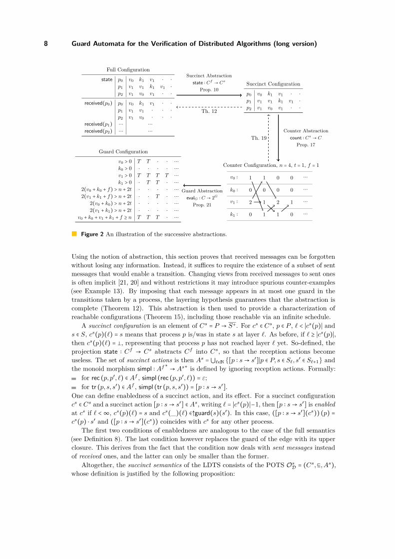
Figure 2 An illustration of the successive abstractions.

Using the notion of abstraction, this section proves that received messages can be forgottenwithout losing any information. Instead, it suffices to require the existence of a subset of sentmessages that would enable a transition. Changing views from received messages to sent onesis often implicit [21, 20] and without restrictions it may introduce spurious counter-examples(see Example 13). By imposing that each message appears in at most one guard in thetransitions taken by a process, the layering hypothesis guarantees that the abstraction iscomplete (Theorem 12). This abstraction is then used to provide a characterization ofreachable configurations (Theorem 15), including those reachable via an infinite schedule.

A succinct configuration is an element of Cs = P → S+. For cs ∈ Cs, p ∈ P , ℓ < ∣cs(p)∣ ands ∈ S, cs(p)(ℓ) = s means that process p is/was in state s at layer ℓ. As before, if ℓ ≥ ∣cs(p)∣,then cs(p)(ℓ) = �, representing that process p has not reached layer ℓ yet. So-defined, theprojection state ∶ Cf → Cs abstracts Cf into Cs, so that the reception actions becomeuseless. The set of succinct actions is then As = ⋃ℓ∈N {[p ∶ s→ s′]∣p ∈ P, s ∈ Sℓ, s

′ ∈ Sℓ+1} andthe monoid morphism simpl ∶ Af∗ → As∗ is defined by ignoring reception actions. Formally:

for rec (p, p′, ℓ) ∈ Af , simpl (rec (p, p′, ℓ)) = ε;for tr (p, s, s′) ∈ Af , simpl (tr (p, s, s′)) = [p ∶ s→ s′].

One can define enabledness of a succinct action, and its effect. For a succinct configurationcs ∈ Cs and a succinct action [p ∶ s→ s′] ∈ As, writing ℓ = ∣cs(p)∣−1, then [p ∶ s→ s′] is enabledat cs if ℓ <∞, cs(p)(ℓ) = s and cs(_)(ℓ) ∈↑guard(s)(s′). In this case, ([p ∶ s→ s′](cs)) (p) =cs(p) ⋅ s′ and ([p ∶ s→ s′](cs)) coincides with cs for any other process.

The first two conditions of enabledness are analogous to the case of the full semantics(see Definition 8). The last condition however replaces the guard of the edge with its upperclosure. This derives from the fact that the condition now deals with sent messages insteadof received ones, and the latter can only be smaller than the former.

Altogether, the succinct semantics of the LDTS consists of the POTS OsD = (Cs,⊑,As),

whose definition is justified by the following proposition:


▶ Proposition 10. The mappings state ∶ Cf → Cs and simpl ∶ Af∗ → As∗ define an abstractionfrom the full POTS Of

D = (Cf ,⊑,Af) to the succinct POTS Os

D = (Cs,⊑,As).

▶ Example 11. Consider the succinct configuration cs in the top right of Figure 2. Itis obtained by applying state to the full configuration cf on the left. In Example 9, thefull schedule σf = rec (p0, p2,2) ⋅ rec (p0, p1,2) ⋅ tr (p0, v1, v1) is shown to be applicable at cf .Therefore, Proposition 10 implies that simpl(σf) = [p0 ∶ v1 → v1] is applicable at cs.

Propositions 10 and 5 entail that the succinct abstraction is sound in the sense that it doesnot remove any existing behavior, and properties that hold on every execution of the succinctmodel also hold on the full semantics. However, in general, abstractions are not completeand they may introduce new behaviors (for instance, schedules without any reception actionsmay be applicable in the simplification but not in the full model). Nevertheless, the succinctabstraction is complete: there always exists an applicable full schedule corresponding to eachapplicable succinct schedule.

▶ Theorem 12. Let σs ∈ As∗ be a succinct schedule applicable at an initial configurationcs ∈ Cs. Then, there exists a full schedule σf ∈ Af∗ applicable at a full configuration cf ∈ Cf

such that: state(cf) = cs, simpl(σf) = σs, and state(cf ⋆ σf) = cs ⋆ σs.

To prove Theorem 12 one transforms each action [p ∶ s→ s′] into a finite schedule ofthe form (rec (p, pu, ℓ))u<U ⋅ tr (p, s, s′), carefully choosing the receptions to ensure that thelast transition is enabled. To do so, the difficulties are twofold. First, the full schedule(rec (p, pu, ℓ))u<U ⋅ tr (p, s, s′) not only depends on [p ∶ s→ s′], but also on the current con-figuration. Therefore one cannot define a trivial abstraction. Second, this method requiresa way to control the buffers of received messages throughout the schedule. Indeed, oneshould avoid that a process receives too many messages to take a transition, as ‘un-receiving’messages in impossible. This is where the layered structure comes into play, and ensures thatwhen a process receives messages enabling a transition, no earlier transition required these.

▶ Example 13. As explained, the layering assumption is crucial in Theorem 12. Consider thenon layered distributed transition system with four states a, b, c, x, and two processes p, p′. Letcf be the initial full configuration with state(cf)(p) = a and state(cf)(p′) = x. Intuitively, inthis counterexample, the guards are set such that the first transition tr (p, a, b) is enabled onlyif received(cf)(p)(p′) = x while the next transition tr (p, b, c) requires received(cf)(p)(p′) =� ≠ x. Process p would thus have to ‘forget’ that it received a message from p′ in order totake the second transition, which is impossible in the full semantics.

In contrast, the succinct semantics does not record whether p has already received themessage from p′ when approaching the second transition. The succinct schedule [p ∶ a→ b] ⋅[p ∶ b→ c] is therefore applicable at state(cf) which would contradict Theorem 12 for unlayereddistributed transition systems. Imposing that each message appears at most in one guardalong the execution of a process, the layered hypothesis prevents this type of counterexamples.

The advantage of the succinct semantics over the full one is that the guards can onlybecome true during an execution. This monotony property, combined with the layeredhypothesis, entail the possibility to check that a configuration is reachable a posteriori,simply by verifying that the guards of the transitions that are taken are verified in the lastconfiguration. In particular, this avoids building explicitly the schedule at all intermediateconfigurations. This is formally stated in the following definition and theorem.

▶ Definition 14. A succinct configuration cs ∈ Cs is coherent if for any p ∈ P and ℓ ∈N, ifcs(p)(ℓ) = s ≠ � and cs(p)(ℓ + 1) = s′ ≠ �, then cs(_)(ℓ) ∈↑guard(s, s′).


▶ Theorem 15. Let cs, cs′ ∈ Cs be two succinct configurations such that cs is coherent. Thenthe following statements are equivalent:

cs ⊑ cs′ and cs′ is coherent.There exists a (possibly infinite) schedule σs ∈ As∗ applicable at cs such that cs ⋆ σs = cs′.

3.3 Counter AbstractionThe theory presented so far dealt with a fixed set P of processes. As an advantage, theguards of the edges could be any condition on the set of received messages, but as a drawback,it is impossible to represent parameterised systems where the number of processes is notfixed. To remedy this downside, this section introduces layered threshold automata (LTA).While this model is syntactically similar to threshold automata [20], its semantics in termsof a POTS is novel. Natural abstractions between the semantics of LDTS and LTA can thenbe presented, proving that LTA form a faithful representation of distributed algorithms, incontrast to unrestricted threshold automata.

▶ Definition 16. A Layered Threshold Automaton (LTA) is a tuple T = (R,S,guard) where:R is a set of parametersS is a set of states partitioned into layers: S = ⋃∞i=0 Si, with S0 the set of initial states.guard ∶ S2 → PA(S ∪R) associates a guard, in Presburger arithmetic over free variablesin S ∪R, to each pair of states. The layered hypothesis assumes that for ℓ ∈ N, s ∈ Sℓ,and s′ ∈ S, guard(s, s′) ∈ PA(Sℓ ∪R) and if s′ ∉ Sℓ+1, guard(s, s′) = false.

The guards are monotonous, i.e. for any guard g ∈ guard(S2), for any valuation ρ ∈ NR,κ,κ′ ∈NS, if κ ≤ κ′ when ordered pointwise and if ρ, κ ⊧ g, then ρ, κ′ ⊧ g as well.

The set of parameters R typically includes the number n of processes and an upper boundt on the number of faulty processes. Intuitively, the guards represent the conditions onsent messages for taking the corresponding transition. The monotony assumption thereforerequires that guards in the algorithms concern received messages only, which may be anysubset of the sent messages.

In the remainder of this section, T = (R,S,guard) is a fixed LTA. A configuration c of Tis defined by:

a parameter valuation param(c) ∈ R →N that remains constant during an execution;a counting mapping κ(c) ∈ S →N where κ(c)(s) = k means that k processes have visitedthe state s;flow counters flow(c) ∈ (⋃ℓ∈N Sℓ × Sℓ+1) → N where flow(c)(s, s′) = k means that kprocesses moved from s to s′.

Moreover, processes that leave a state must have entered it, therefore, configuations shouldalso verify the following flow conditions:- in: for every ℓ ∈N ∖ {0} and every s ∈ Sℓ, ∑s′∈Sℓ−1 flow(c)(s

′, s) = κ(c)(s)- out: for every ℓ ∈N and every s ∈ Sℓ, ∑s′∈Sℓ+1 flow(c)(s, s

′) ≤ κ(c)(s).The set C of all configurations is equipped with the natural order ⊑ defined by c ⊑ c′ ifparam(c) = param(c′), κ(c) ≤ κ(c′) and flow(c) ≤ flow(c′).

An action over C is an element ofA = ⋃ℓ∈NAℓ where for ℓ ∈N, Aℓ = {[s→ s′]∣s ∈ sℓ, s′ ∈ Sℓ+1}.

For c ∈ C, an action [s→ s′] ∈ Aℓ is enabled at c if:∑s′′∈Sℓ+1 flow(c)(s, s

′′) < κ(c)(s), andparam(c), κ(c) ⊧ guard(s, s′), written c ⊧ guard(s, s′) for short.

In so, the successor configuration [s→ s′] (c) = c′ ∈ C is defined by:param(c′) = param(c)flow(c′) = flow(c) + 1(s,s′) where 1(s,s′)(s, s′) = 1 and 1(s,s′)(e) = 0 elsewhere.


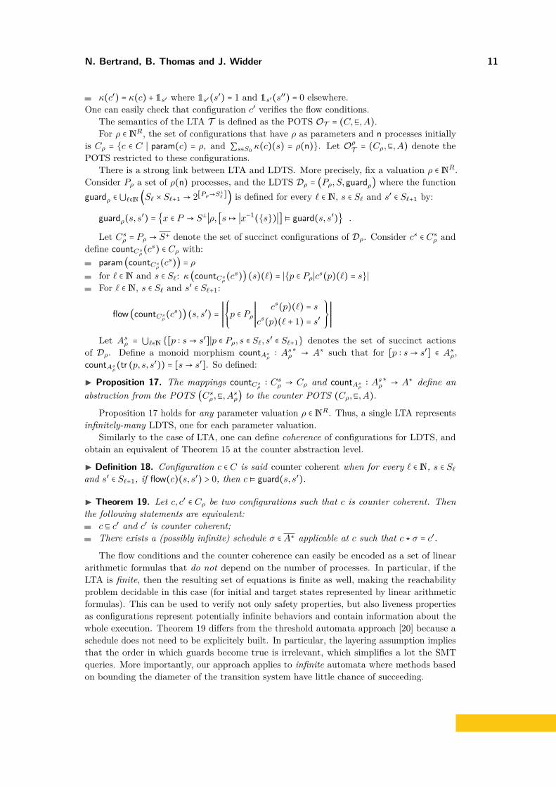
κ(c′) = κ(c) + 1s′ where 1s′(s′) = 1 and 1s′(s′′) = 0 elsewhere.One can easily check that configuration c′ verifies the flow conditions.

The semantics of the LTA T is defined as the POTS OT = (C,⊑,A).For ρ ∈NR, the set of configurations that have ρ as parameters and n processes initially

is Cρ = {c ∈ C ∣ param(c) = ρ, and ∑s∈S0 κ(c)(s) = ρ(n)}. Let OρT = (Cρ,⊑,A) denote the

POTS restricted to these configurations.There is a strong link between LTA and LDTS. More precisely, fix a valuation ρ ∈NR.

Consider Pρ a set of ρ(n) processes, and the LDTS Dρ = (Pρ, S,guardρ) where the functionguardρ ∈ ⋃ℓ∈N (Sℓ × Sℓ+1 → 2[Pρ→S�ℓ ]) is defined for every ℓ ∈N, s ∈ Sℓ and s′ ∈ Sℓ+1 by:

guardρ(s, s′) = {x ∈ P → S�∣ρ, [s↦ ∣x−1({s})∣] ⊧ guard(s, s′)} .

Let Csρ = Pρ → S+ denote the set of succinct configurations of Dρ. Consider cs ∈ Cs

ρ anddefine countCs

ρ(cs) ∈ Cρ with:

param (countCsρ(cs)) = ρ

for ℓ ∈N and s ∈ Sℓ: κ (countCsρ(cs)) (s)(ℓ) = ∣{p ∈ Pρ∣cs(p)(ℓ) = s}∣

For ℓ ∈N, s ∈ Sℓ and s′ ∈ Sℓ+1:

flow (countCsρ(cs)) (s, s′) =

RRRRRRRRRRR

⎧⎪⎪⎨⎪⎪⎩p ∈ Pρ

RRRRRRRRRRR

cs(p)(ℓ) = scs(p)(ℓ + 1) = s′

⎫⎪⎪⎬⎪⎪⎭

RRRRRRRRRRRLet As

ρ = ⋃ℓ∈N {[p ∶ s→ s′]∣p ∈ Pρ, s ∈ Sℓ, s′ ∈ Sℓ+1} denotes the set of succinct actions

of Dρ. Define a monoid morphism countAsρ∶ As

ρ∗ → A∗ such that for [p ∶ s→ s′] ∈ As

ρ,countAs

ρ(tr (p, s, s′)) = [s→ s′]. So defined:

▶ Proposition 17. The mappings countCsρ∶ Cs

ρ → Cρ and countAsρ∶ As

ρ∗ → A∗ define an

abstraction from the POTS (Csρ ,⊑,As

ρ) to the counter POTS (Cρ,⊑,A).

Proposition 17 holds for any parameter valuation ρ ∈NR. Thus, a single LTA representsinfinitely-many LDTS, one for each parameter valuation.

Similarly to the case of LTA, one can define coherence of configurations for LDTS, andobtain an equivalent of Theorem 15 at the counter abstraction level.

▶ Definition 18. Configuration c ∈ C is said counter coherent when for every ℓ ∈N, s ∈ Sℓ

and s′ ∈ Sℓ+1, if flow(c)(s, s′) > 0, then c ⊧ guard(s, s′).

▶ Theorem 19. Let c, c′ ∈ Cρ be two configurations such that c is counter coherent. Thenthe following statements are equivalent:

c ⊑ c′ and c′ is counter coherent;There exists a (possibly infinite) schedule σ ∈ A∗ applicable at c such that c ⋆ σ = c′.

The flow conditions and the counter coherence can easily be encoded as a set of lineararithmetic formulas that do not depend on the number of processes. In particular, if theLTA is finite, then the resulting set of equations is finite as well, making the reachabilityproblem decidable in this case (for initial and target states represented by linear arithmeticformulas). This can be used to verify not only safety properties, but also liveness propertiesas configurations represent potentially infinite behaviors and contain information about thewhole execution. Theorem 19 differs from the threshold automata approach [20] because aschedule does not need to be explicitely built. In particular, the layering assumption impliesthat the order in which guards become true is irrelevant, which simplifies a lot the SMTqueries. More importantly, our approach applies to infinite automata where methods basedon bounding the diameter of the transition system have little chance of succeeding.


v0 v1 accv1 ≥ t + 1 − f v1 ≥ n − t − f

(a) Non-layered v0

v1

x acc

v1 ≥ t +1 − f x ≥ n − t − f

(b) Layered

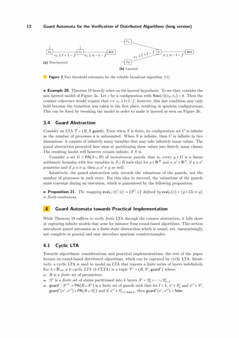
Figure 3 Two threshold automata for the reliable broadcast algorithm [11].

▶ Example 20. Theorem 19 heavily relies on the layered hypothesis. To see that, consider thenon layered model of Figure 3a. Let c be a configuration with flow(c)(v0, v1) > 0. Then thecounter coherence would require that c ⊧ v1 ≥ t+1−f , however, this last condition may onlyhold because the transition was taken in the first place, resulting in spurious configurations.This can be fixed by tweaking the model in order to make it layered as seen on Figure 3b.

3.4 Guard AbstractionConsider an LTA T = (R,S,guard). Even when S is finite, its configuration set C is infiniteas the number of processes n is unbounded. When S is infinite, then C is infinite in twodimensions: it consists of infinitely many variables that may take infinitely many values. Theguard abstraction presented here aims at partitioning these values into finitely many classes.The resulting model will however remain infinite, if S is.

Consider a set G ⊂ PA(S ∪ R) of monotonous guards, that is, every g ∈ G is a lineararithmetic formulas with free variables in S ∪R such that for ρ ∈NR and κ,κ′ ∈NS , if κ ≤ κ′pointwise and if ρ, κ ⊧ g, then ρ, κ′ ⊧ g as well.

Intuitively, the guard abstraction only records the valuations of the guards, not thenumber of processes in each state. For this idea to succeed, the valuations of the guardsmust converge during an execution, which is guaranteed by the following proposition.

▶ Proposition 21. The mapping evalG∶ (C,⊑) → (2G,⊆) defined by evalG(c) = {g ∈ G∣c ⊧ g}is Scott-continuous.

4 Guard Automata towards Practical Implementation

While Theorem 19 suffices to verify finite LTA through the counter abstraction, it falls shortat capturing infinite models that arise for instance from round-based algorithms. This sectionintroduces guard automata as a finite-state abstraction which is sound, yet, unsurprisingly,not complete in general and may introduce spurious counterexamples.

4.1 Cyclic LTATowards algorithmic considerations and practical implementations, the rest of the paperfocuses on round-based distributed algorithms, which can be captured by cyclic LTA. Intuit-ively, a cyclic LTA is used to model an LTA that repeats a finite series of layers indefinitely.For k ∈N>0, a k-cyclic LTA (k-CLTA) is a tuple T c = (R,Sc,guardc) where:

R is a finite set of parameters.Sc is a finite set of states partitioned into k layers Sc = Sc

0 ∪⋯ ∪ Sck−1.

guardc ∶ Sc2 → PA(R∪Sc) is a finite set of guards such that for ℓ < k, sc ∈ Scℓ and sc′ ∈ Sc,

guardc(sc, sc′) ∈ PA(R ∪ Scℓ) and if sc′ ∉ Sc

ℓ+1 mod k, then guardc(sc, sc′) = false.


Unfolding a k-CLTA yields an infinite-state acyclic LTA unfold (R,Sc,guardc). Formallyunfold (R,Sc,guardc) = (R,S,guard) with:

S = {(sc, ℓ) ∣ ℓ ∈N, sc ∈ Scℓ mod k}

For ℓ ∈N, sc ∈ Scℓ mod k and sc′ ∈ Sc

ℓ+1 mod k, guard ((sc, ℓ), (sc′, ℓ + 1)) = guardc(sc, sc′)[sc′′ ←(sc′′, ℓ) for sc′′ ∈ Sc

ℓ mod k] meaning that any free variable sc′′ ∈ Sc that appears inguardc(sc, sc′) gets replaced with (sc′′, ℓ). In any other case, guard is false.

4.2 Guard AutomatonFrom the guard abstraction, one can construct a finite-state automaton that represents theset of reachable configurations of a cyclic LTA.

Let T c = (R,Sc,guardc) be a k-CLTA equipped with a finite set of guards expressed inPresburger arithmetic: Gc = ⋃ℓ<k G

cℓ such that for ℓ < k, Gc

ℓ ∈ PA(Scℓ ∪R). In practice, Gc

will include all guards appearing in the LTA, as well as the events that need to be observed.A CLTA can be unfolded into an infinite-state LTA, by concatenating copies of T c. In

order for the guard abstraction to be formally defined, copies of the guards in Gc for each newlayer are required. For ℓ ∈N a layer index and gc ∈ Gc

ℓ mod k a guard, unfoldGℓ(gc) = gc[sc ←

(sc, ℓ) for sc ∈ Scℓ mod k] denotes the guard obtained by replacing every free occurrence of

a variable sc ∈ Scℓ mod k in gc by (sc, ℓ). The converse folding operation is defined by:

foldGℓ(g) = g[(sc, ℓ) ← sc, for sc ∈ Sc

ℓ mod k]. Finally, Gℓ = unfoldG (Gcℓ mod k) is the set of

guards at layer ℓ and G = ⋃ℓ∈NGℓ the set of all guards.The guard abstraction maps every configuration of unfold(T c) to a set of guards that hold

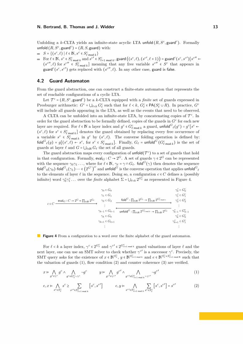
in that configuration. Formally, evalG ∶ C → 2G. A set of guards γ ∈ 2G can be representedwith the sequence γ0γ1 . . . , where for ℓ ∈N, γℓ = γ ∩Gℓ. foldG(γ) then denotes the sequencefoldG

0(γ0) ⋅foldG1(γ1) ⋅⋯ ∈ (2Gc

)ω and unfoldG is the converse operation that applies unfoldGℓ

to the elements of layer ℓ in the sequence. Doing so, a configuration c ∈ C defines a (possiblyinfinite) word γc

0γc1 . . . over the finite alphabet Σ = ⋃ℓ<k 2Gc

ℓ as represented in Figure 4.

c ∈ C

γ0 ⊂ G0

γ1 ⊂ G1

γ2 ⊂ G2

⋮γk−1 ⊂ Gk−1

γk ⊂ Gk

γk+1 ⊂ Gk+1

⋮

γc0 ⊂ Gc

0

γc1 ⊂ Gc

1

γc2 ⊂ Gc

2

⋮γc

k−1 ⊂ Gck−1

γck ⊂ Gc

0

γck+1 ⊂ Gc

1

⋮

evalG ∶ C → 2G ≈∏ℓ∈N 2Gℓ foldG ∶∏ℓ∈N 2Gℓ →∏ℓ∈N 2Gcℓ mod k

unfoldG ∶∏ℓ∈N 2Gcℓ mod k →∏ℓ∈N 2Gℓ

Figure 4 From a configuration to a word over the finite alphabet of the guard automaton.

For ℓ < k a layer index, γc ∈ 2Gcℓ and γc′ ∈ 2Gc

ℓ+1 mod k guard valuations of layer ℓ and thenext layer, one can use an SMT solver to check whether γc′ is a successor γc. Precisely, theSMT query asks for the existence of x ∈ NSc

ℓ , y ∈ NScℓ+1 mod k and e ∈ NSc

ℓ×Scℓ+1 mod N such that

the valuation of guards (1), flow condition (2) and counter coherence (3) are verified.

x ⊧ ⋀gc∈γc

gc ∧ ⋀gc∈Gc

ℓ∖γc

¬gc y ⊧ ⋀gc′∈γc′

gc′ ∧ ⋀gc′∈Gc

ℓ+1 mod k∖γc′

¬gc′ (1)

e, x ⊧ ⋀sc∈Sc

ℓ

sc ≥ ∑sc′∈Sc

ℓ+1 mod k

[sc, sc′] e, y ⊧ ⋀sc′∈Sc

ℓ+1 mod k

∑sc∈Sc

ℓ

[sc, sc′] = sc′ (2)


e, x ⊧ ⋀(sc,sc′)∈Sc

ℓ×Sc

ℓ+1 mod N

[sc, sc′] > 0Ð→ guardc(sc, sc′) (3)

The guard automaton is a finite automaton whose language overapproximates the setof reachable configurations. It bears similarities with de Bruijn graphs [15] used e.g. inbioinformatics. If Eℓ ⊂ 2Gc

ℓ ×2Gcℓ+1 mod k denotes the set of all pairs γc, γc′ that verify conditions

(1) and and (3), one can build the set E = ⋃ℓ<k Eℓ.

▶ Definition 22. The guard automaton of T c is GAG(T c) = (Σ,E,2Gc0 , src,dest, label) where:

Σ is both the alphabet and the set of states.2Gc

0 ⊂ Σ is the set of initial states.E ⊂ Σ2 defined above is the set of edges, equipped with src ∶ E → Σ (resp. dest ∶ E → Σ)that defines the source state (resp. destination state) of every edge, and label ∶ E → Σassociates a label to each edge defined by label(γc, γc′) = γc.

An infinite run (eℓ)ℓ<∞ of the guard automaton defines a word word ((eℓ)ℓ<∞) = label(e0) ⋅label(e1) ⋅ ⋯ , and L(GAG(T c)) ⊂ Σω denotes the language of GAG(T c).

▶ Example 23. Algorithm 1 can be described by the following CLTA with k = 1. Theparameters are R = {n, t, f} where f denotes the actual number of Byzantine faults. Statesare Sc = {v0, k0, v1, k1}. The guards here only depend on the next value of v. For instance:

guard(_, v0) = (v0 + k0 + v1 + k1 + f = n)

∧ ((2(v0 + k0 + f) > n + 2t) ∨ ((2v0 + 2k0 ≤ n + 2t) ∧ (2v1 + 2k1 ≤ n + 2t) ∧ (k1 = 0))).

Also, guard(_, k0) = guard(_, v0) and guard(_, v1) = guard(_, k1) is defined symmetrically.A configuration c of the unfolded LTA is depicted bottom-right of Figure 2, where the array

contains the valuation κ(c) and the arrows represent the flow. For example κ(c)(v1,0) = 2,flow(c)((v0,0), (k1,1)) = 1 and flow(c)((v0,0), (v0,1)) = 0.

The guard abstraction transforms c into the guard configuration bottom-left of Figure 2.Here, we chose the set of guards Gc to consist of s > 0 for each s ∈ Sc and of the guardsof the LTA. The alphabet Σ contains e.g., (T ⋅ T ⋅ ⋅ ⋅ ⋅ ⋅ T ). SMT queries determine whethertwo letters may appear successively, in order to build the guard automaton. For instance,according to the first two layers of evalG(c), (T ⋅ T ⋅ ⋅ ⋅ ⋅ ⋅ T ) can be followed by (T ⋅ TT ⋅ ⋅ ⋅ ⋅T ).There will therefore be a transition between these two states in the guard automaton.

▶ Theorem 24. Let c ∈ C be a configuration of unfold(T c) and evalG(c) ∈ 2G its guardabstraction. If c is counter-coherent, then foldG (evalG(c)) ∈ L(GAG(T c)).

By soundness of the guard automaton construction, a property which holds on configur-ations that correspond to runs of GAG(T c) also holds on the configurations of unfold(T c).A simple verification procedure thus consists in checking that L(GAG(T c)) is included in agiven language of correct configurations. At a first glance, it might seem that only safetyproperties can be checked. However, the guard automaton also represents configurationsreachable by infinite schedules, making the verification of liveness properties feasible.

▶ Example 25. For presentation purposes, Algorithm 1 is an overly simplified version ofthe Phase King algorithm [8]. The latter can be faithfully encoded by the 2-CLTA T c ofFigure 5, where the updated value when there is no clear majority is not the king’s value,but rather the majority of the values received by the king. Each round consists of twolayers of communication, a first in which each process broadcasts its value, and a second in


v0

v1

k0,0

k0,1

p0

p1

k1,0

k1,1

v0

v1

P = {n, t, f} and for x, y ∈ {0,1}:

guard(vx, px) = trueguard(vx, kx,y) = [2(vy + f) ≥ n]guard(_, vx) = [2(px + kx,0 + kx,1) > n + 2t]∨

⎡⎢⎢⎢⎢⎢⎢⎣

2(p0 + k0,0 + k0,1) ≤ n + 2t∧2(p1 + k1,0 + k1,1) ≤ n + 2t∧

k0,x + k1,x = 0

⎤⎥⎥⎥⎥⎥⎥⎦

Figure 5 A 2-CLTA for the Phase King algorithm with non-deterministic choice of the king. Aprocess in kx,y is king of the current round, its current value is x and it thinks the majority is y.

which the king broadcasts what it thinks is the majority. The set of guards at the first layeris Gc

0 = {v0 > 0, v1 > 0} and at the second layer Gc1 consists of k0,0+k1,0 > 0, k0,1+k1,1 > 0,

p0+k0,0+k0,1 > 0, p1+k1,0+k1,1 > 0, 2(k0,0+k0,1+p0+f) > n+2t and 2(k1,0+k1,1+p1+f) > n+2t.Restricting to valuations with ∑s∈Sℓ

s+f = n (fairness) and k0,0+k0,1+k1,0+k1,1 ≤ 1 (atmost one king), the resulting guard automaton has 3 states in even layers and 11 in oddlayers. Writing [formula] for the set of letters in 2Gc

for which formula holds, one can show:

L(GAG(T c)) ⊂ [¬(k0,0 + k1,0 > 0) ∧ ¬(k0,1 + k1,1 > 0)]ω (4)∪Σ∗[(k0,0 + k1,0 > 0) ∨ (k0,1 + k1,1 > 0)][¬(p0 + k0,0 + k0,1 > 0)]ω (5)∪Σ∗[(k0,0 + k1,0 > 0) ∨ (k0,1 + k1,1 > 0)][¬(p1 + k1,0 + k1,1 > 0)]ω . (6)

Therefore, either every chosen king is Byzantine (4), or all processes agree on a value after anon-Byzantine king is chosen (5 or 6).

In general, although is it sound, the guard automaton construction is not complete: thelanguage may contain words that correspond to no configuration of the LTA. As usual forincomplete methods, heuristics can be used to remove some spurious counterexamples.

5 Conclusion

This paper presented a methodology, based on domain theory, to represent and analyzedistributed algorithms. Infinite-state models are abstracted into finite-state guard automata,on which one can check safety and liveness properties.

Optimizing and benchmarking the guard automaton implementation is on our currentagenda to demonstrate the applicability of our methodology by verifying safety and livenessof standard distributed algorithms from the literature. A more long-term research objectiveis to build on the current contribution to develop a rigorous framework for the verification ofrandomized distributed algorithms.

References1 Parosh Aziz Abdulla, Mohamed Faouzi Atig, Zeinab Ganjei, Ahmed Rezine, and Yunyun

Zhu. Verification of cache coherence protocols wrt. trace filters. In Proceedings of the 15thInternational Conference on Formal Methods in Computer-Aided Design (FMCAD’15), pages9–16. IEEE, 2015.

2 Samson Abramsky and Achim Jung. Domain Theory, volume 3 of Handbook of Logic inComputer Science. Clarendon Press, 1994.


3 C. Aiswarya, Benedikt Bollig, and Paul Gastin. An automata-theoretic approach to theverification of distributed algorithms. Information and Computation, 259:305–327, 2018.

4 Francesco Alberti, Silvio Ghilardi, and Elena Pagani. Counting constraints in flat arrayfragments. In Proceedings of the 8th International Joint Conference on Automated Reasoning(IJCAR’16), volume 9706 of Lecture Notes in Computer Science, pages 65–81, 2016.

5 A. R. Balasubramanian, Javier Esparza, and Marijana Lazić. Complexity of verification andsynthesis of threshold automata. In Proceedings of the 18th International Symposium onAutomated Technology for Verification and Analysis (ATVA’20), volume 12302 of LectureNotes in Computer Science, pages 144–160. Springer, 2020.

6 Michael Ben-Or. Another advantage of free choice: Completely asynchronous agreementprotocols (extended abstract). In Proceedings of the 2nd Annual ACM SIGACT-SIGOPSSymposium on Principles of Distributed Computing (PODC’83), pages 27–30, 1983.

7 Idan Berkovits, Marijana Lazic, Giuliano Losa, Oded Padon, and Sharon Shoham. Verificationof threshold-based distributed algorithms by decomposition to decidable logics. In Proceedingsof the 31st International Conference on Computer Aided Verification (CAV’19), volume 11562of Lecture Notes in Computer Science, pages 245–266. Springer, 2019.

8 Piotr Berman and Juan A. Garay. Cloture votes: n/4-resilient distributed consensus in t+1rounds. Mathematical Systems Theory, 26(1):3–19, 1993.

9 Roderick Bloem, Swen Jacobs, Ayrat Khalimov, Igor Konnov, Sasha Rubin, Helmut Veith, andJosef Widder. Decidability of Parameterized Verification. Synthesis Lectures on DistributedComputing Theory. Morgan & Claypool Publishers, 2015.

10 Luca Bortolussi and Jane Hillston. Model checking single agent behaviours by fluid approxim-ation. Information and Computation, 242:183–226, 2015.

11 Gabriel Bracha and Sam Toueg. Asynchronous consensus and broadcast protocols. Journal ofthe ACM, 32(4):824–840, 1985.

12 Mouna Chaouch-Saad, Bernadette Charron-Bost, and Stephan Merz. A reduction theorem forthe verification of round-based distributed algorithms. In Proceedings of the 3rd InternationalWorkshop on Reachability Problems (RP’09), volume 5797 of Lecture Notes in ComputerScience, pages 93–106, 2009.

13 Bernadette Charron-Bost and André Schiper. The heard-of model: computing in distributedsystems with benign faults. Distributed Computing, 22(1):49–71, 2009.

14 Andrei Damian, Cezara Drăgoi, Alexandru Militaru, and Josef Widder. Communication-closedasynchronous protocols. In Proceedings of the 31st International Conference on ComputerAided Verification (CAV’19), volume 11562 of Lecture Notes in Computer Science, pages344–363. Springer, 2019.

15 Nicolaas G. de Bruijn. A combinatorial problem. Indagationes Mathematicae, 49:758–764,1946.

16 Cezara Drăgoi, Thomas A. Henzinger, Helmut Veith, Josef Widder, and Damien Zufferey. ALogic-Based Framework for Verifying Consensus Algorithms. In Proceedings of the 15th Inter-national Conference on Verification, Model Checking, and Abstract Interpretation (VMCAI’14),volume 8318 of Lecture Notes in Computer Science, pages 161–181, 2014.

17 Tzilla Elrad and Nissim Francez. Decomposition of distributed programs into communication-closed layers. Science of Computer Programming, 2(3):155–173, 1982.

18 Javier Esparza. Keeping a crowd safe: On the complexity of parameterized verification (invitedtalk). In Proceedings of the 31st International Symposium on Theoretical Aspects of ComputerScience (STACS’14), volume 25 of LIPIcs, pages 1–10. Schloss Dagstuhl - Leibniz-Zentrumfuer Informatik, 2014.

19 Igor Konnov, Marijana Lazić, Helmut Veith, and Josef Widder. A short counterexampleproperty for safety and liveness verification of fault-tolerant distributed algorithms. InProceedings of the 44th ACM SIGPLAN Symposium on Principles of Programming Languages(POPL’17), pages 719–734, 2017.


20 Igor Konnov, Helmut Veith, and Josef Widder. On the completeness of bounded model checkingfor threshold-based distributed algorithms: Reachability. Information and Computation, 252:95–109, 2017.

21 Jure Kukovec, Igor Konnov, and Josef Widder. Reachability in parameterized systems:All flavors of threshold automata. In Proceedings of the 29th International Conference onConcurrency Theory (CONCUR’18), volume 118 of LIPIcs, pages 19:1–19:17, 2018.

22 Leslie Lamport. Checking a multithreaded algorithm with +CAL. In Proceedings of the 20thInternational Symposium on Distributed Computing (DISC’06), volume 4167 of Lecture Notesin Computer Science, pages 151–163. Springer, 2006.

23 Richard J. Lipton. Reduction: A method of proving properties of parallel programs. Commu-nications of the ACM, 18(12):717–721, 1975.

24 Ognjen Maric, Christoph Sprenger, and David A. Basin. Cutoff bounds for consensus algorithms.In Proceedings of the 29th International Conference on Computer Aided Verification (CAV’17),volume 10427 of Lecture Notes in Computer Science, pages 217–237, 2017.

25 Kenneth L. McMillan. Parameterized verification of the FLASH cache coherence protocol bycompositional model checking. In Proceedings of the 11th IFIP WG 10.5 Advanced ResearchWorking Conference on Correct Hardware Design and Verification Methods (CHARME’01),volume 2144, pages 179–195. Springer, 2001.

26 Dominique Méry. Verification by Construction of Distributed Algorithms. In Proceedings ofthe 16th International Colloquium on Theoretical Aspects of Computing (ICTAC’19), volume11884 of Lecture Notes in Computer Science, pages 22–38. Springer, 2019.

27 Arnaud Sangnier, Nathalie Sznajder, Maria Potop-Butucaru, and Sébastien Tixeuil. Para-meterized verification of algorithms for oblivious robots on a ring. In Proceedings of the 17thInternational Conference on Formal Methods in Computer Aided Design (FMCAD’17), pages212–219. IEEE, 2017.

28 Ocan Sankur and Jean-Pierre Talpin. An abstraction technique for parameterized modelchecking of leader election protocols: Application to FTSP. In Proceedings of the 23rdInternational Conference on Tools and Algorithms for the Construction and Analysis ofSystems (TACAS’17), volume 10205 of Lecture Notes in Computer Science, pages 23–40, 2017.doi:10.1007/978-3-662-54577-5_2.

29 Ilina Stoilkovska, Igor Konnov, Josef Widder, and Florian Zuleger. Verifying safety ofsynchronous fault-tolerant algorithms by bounded model checking. In Proceedings of the25th International Conference on Tools and Algorithms for the Construction and Analysis ofSystems (TACAS’19), volume 11428 of Lecture Notes in Computer Science, pages 357–374,2019.

https://doi.org/10.1007/978-3-662-54577-5_2


Technical appendix

A Complements for Section 2

Proof of Lemma 3

▶ Lemma 3. For x ∈X, the set App(x) of schedules applicable at x is Scott-closed for theprefix ordering and the function: [x ⋆_] ∶ App(x)→X is Scott-continuous.

Proof. Two points need to be shown: first, that the set App(x) ⊂ A∗ is Scott-closed, andsecond, that the function [x ⋆_] ∶ App(x)→X is Scott-continuous.

A Scott-closed set is a set that is both downward-closed and closed by least upper boundof directed subsets. The set App(x) is downward-closed as any prefix of an applicableschedule is applicable as well.Consider a directed set ζ ⊂ App(x), The set ζ consists of prefixes of the schedule ⊔ ζ thatare applicable at x. Then ↓ζ ⊂ App(x) must contain at least the finite prefixes of ⊔ ζ.All the finite prefixes of ⊔ ζ are then applicable, and this condition implies that ⊔ ζ itselfis applicable.Therefore, App(x) is Scott-closed.The function [x ⋆ _] is monotonous. Indeed, consider two schedules σ,σ′ ∈ A∗ bothapplicable at x and suppose σ ≺ σ′. Then, either σ = σ′ in which case x⋆σ ⊑ x⋆σ′ clearlyholds, or σ is finite and there exists σ′′ ∈ A∗ such that σ ⋅σ′′ = σ′. Then x⋆σ′ = (x⋆σ)⋆σ′′and x ⋆ σ ⊑ x ⋆ σ′ as the destination of a schedule is always greater than its source.Consider a directed set ζ ⊂ A∗ and define σ = ⊔ ζ. By monotony, ⊔ (x ⋆ ζ) ⊑ x ⋆ σ.Again, ↓ζ contains all the finite prefixes of σ and,

x ⋆ σ =⊔{x ⋆ σt ∣ t ≤ ∣σ∣, t <∞}⊑⊔{x ⋆ σ′ ∣ σ′ ∈↓ζ} because {σt ∣ t ≤ ∣σ∣, t ∈N} ⊂↓ζ⊑⊔[x ⋆_](↓ζ)⊑⊔[x ⋆_](ζ) By monotony of [x ⋆_]

Therefore, ⊔ (x ⋆ ζ) = x ⋆ σ and [x ⋆_] ∶ App(x)→X is Scott-continuous.◀

Proof of Proposition 5

▶ Proposition 5. Let (abX , abA) be an abstraction between O = (X,⊑,A) and O′ = (X ′,⊑,A′),x ∈X be an element, and σ ∈ A∗ a schedule. If σ is applicable at x, then abA(σ) is applicableat abX(x) and abX(x ⋆ σ) = abX(x) ⋆ abA(σ).

Proof. The result can be shown by (transfinite) induction on the length of the schedules.The most involved case is the one of infinite schedules, where continuity of the abstractions(abX and abA), as well as Lemma 3 are used.

If σ = ε, then both σ and abA(σ) = ε are applicable at any configuration. In particular,abX(x ⋆ σ) = abX(x) = abX(x) ⋆ abA(σ).Consider T ∈ N and suppose the result holds for any schedule of length T . Consider aschedule σ = (at)t<T+1 ∈ AT+1 of length T + 1 applicable at a configuration x ∈X. Thennecessarily, the prefix of length T of σ is also applicable at x, and the induction hypothesisgives:


abX (x ⋆ (at)t<T ) = abX(x) ⋆ abA ((at)t<T )

Then, the following holds:

abX (x ⋆ (at)t<T+1) = abX (x ⋆ (at)t<T ⋆ aT )= abX (x ⋆ (at)t<T ) ⋆ abA(aT ) Definition of an abstraction= abX (x) ⋆ abA ((at)t<T ) ⋆ abA(aT ) induction hypothesis= abX (x) ⋆ abA ((at)t<T+1) abA is a monoid morphism

The result therefore holds for any finite schedule.Let now σ be an infinite schedule. For t ∈N, consider σt ∈ At the finite prefix of length tof σ. Then,

abX(x ⋆ σ) = abX (⊔{x ⋆ σt∣t <∞})=⊔{abX (x ⋆ σt)∣t <∞} continuity of abX

=⊔{abX(x) ⋆ abA (σt)∣t <∞} ∣σt∣ <∞= abX(x) ⋆ (⊔{abA (σt)}) Lemma 3= abX(x) ⋆ abA (⊔{σt∣t ∈N}) continuity of abA

= abX(x) ⋆ abA(σ)

This proves the result for infinite schedules, and concludes the induction proof.◀

B Complements for Section 3

B.1 Proofs of Section 3.2Proof of Proposition 10

▶ Proposition 10. The mappings state ∶ Cf → Cs and simpl ∶ Af∗ → As∗ define an abstractionfrom the full POTS Of

D = (Cf ,⊑,Af) to the succinct POTS Os

D = (Cs,⊑,As).

Proof. This proof consists simply of checking that the conditions of Definition 4 are met.

The continuity of state holds as it is a projection.For rec (p, p′, ℓ) ∈ Af and cf ∈ cf , rec (p, p′, ℓ) does not modify the states of the processes.Therefore,

state(cf ⋆ rec (p, p′, ℓ)) = state(cf) ⋆ ε

= state(cf) ⋆ simpl(rec (p, p′, ℓ))

Consider cf ∈ Cf and tr (p, s, s′) ∈ Af applicable at cf .The non-direct part of this proof is to verify that simpl(tr (p, s, s′)) = [p ∶ s→ s′] isapplicable at state(cf). Let ℓ = ∣state(cf)(p)∣−1. The conditions ℓ <∞ and state(cf)(p) =s are directly analogous in both semantics.Because tr (p, s, s′) is applicable at cf , received(cf)(_)(ℓ) ∈ guard(s, s′). Additionally, thedefinition of a full configurations imposes that received(cf)(p)(_)(ℓ) ⊑ state(cf)(_)(ℓ).Therefore, state(cf)(_)(ℓ) ∈↑guard(s, s′) and [p ∶ s→ s′] is indeed enabled at state(cf).


The fact that state(cf ⋆ tr (p, s, s′)) = state(cf) ⋆ [p ∶ s→ s′] follows directly from thedefinition.

Therefore, for any af ∈ Af applicable at a full configuration cf ∈ Cf , simpl(af) is applicableat state(cf) and state(cf ⋆ af) = state(cf) ⋆ simpl(af) which concludes the proof. ◀

Proof of Theorem 12

▶ Theorem 12. Let σs ∈ As∗ be a succinct schedule applicable at an initial configurationcs ∈ Cs. Then, there exists a full schedule σf ∈ Af∗ applicable at a full configuration cf ∈ Cf

such that: state(cf) = cs, simpl(σf) = σs, and state(cf ⋆ σf) = cs ⋆ σs.

The proof of Theorem 12 requires the following lemma:

▶ Lemma B.1. Consider a configuration cf ∈ Cf and an action [p ∶ s→ s′] ∈ As enabled atstate(cf). Additionally, suppose that received(cf)(p)(_)(ℓ) = �. Then there exists σf ∈ Af∗

applicable at cf such that:simpl(σf) = [p ∶ s→ s′] and therefore, state(cf ⋆ σf) = state(cf) ⋆ [p ∶ s→ s′]For any (q, ℓ′) ≠ (p, ℓ), and any q′ ∈ P , received(cf⋆σf)(q)(q′)(ℓ′) = received(cf)(q)(q′)(ℓ′)

Proof. Let ℓ = ∣state(cf)(p)∣ − 1.The fact that [p ∶ s→ s′] is enabled at state(cf) implies ℓ < ∞ and state(cf)(_)(ℓ) ∈↑

guard(s, s′). Therefore, there exists x ∈ guard(s, s′) such that x ⊑ state(cf)(_)(ℓ). Definethe finite sequence (qu)u<U as an enumeration of the set {q ∈ P ∣ x(q) ≠ �} (this set is finitebecause P is finite).

Set σf = (rec (p, qu, ℓ))u<U ⋅ tr (p, s, s′).This schedule is applicable at cf . Indeed, let cf ′ = cf ⋆ (rec (p, qu, )) (ℓ)u<U . Then,

state(cf ′) = state(cf) (reception actions do not alter states) and for q ∈ P , received(cf ′)(p)(q)(ℓ) =state(cf)(q)(ℓ) if q = qu for u < U and is � otherwise. Therefore, received(cf ′)(p)(_)(i) = x ∈guard(s, s′) and tr (p, s, s′) is applicable at cf ′. The whole schedule is then applicable at cf .

The fact that simpl(σf) = [p ∶ s→ s′] is easily verified, and Propositions 5 and 10 concludesthe argument.

Moreover, the reception actions present in the schedules only affect the messages receivedby process p at layer ℓ and none of the other, therefore the second property holds as well. ◀

Proof of Theorem 12. Consider cf ∈ Cf defined with state(cf) = cs and for any p, p′ ∈ Pand ℓ ∈N, received(cf)(p)(p′)(ℓ) = �.

The remainer of the proof consists in creating a partial monotonous function concr ∶As∗ → Af∗ such that:

if σs ∈ As∗ is applicable at cs, concr(σs) ∈ Af∗ is applicable at cf .simpl(concr(σs)) = σs

For σs ∈ As∗ applicable at cs, for any p ∈ P and ℓ ∈N such that no action [p ∶ s→ _] withs ∈ Sℓ appears in σs, received(cf ⋆ concr(σs))(p)(_)(ℓ) = �.

Extending the function concr to a Scott-continuous function on As∗ → Af∗ can then concludethe proof.

The function concr ∶ As∗ → Af∗ is defined inductively as follow:concr(ε) = ε. This clearly satisfies the requirements.For σs ⋅ [p ∶ s→ s′] ∈ As∗, suppose inductively that concr(σs) is defined and fulfill therequirements. Additionally, suppose that σs ⋅ [p ∶ s→ s′] is applicable at cs. Let ℓ ∈N besuch that s ∈ Sℓ. Then there cannot be any action in σs of type [p ∶ s′′ → _] with s′′ ∈ Sℓ.Therefore, by induction hypothesis, received(cf ⋆ concr(σs))(p)(_)(ℓ) = �. The Lemma


above can therefore be used to construct σf ∈ Af∗ applicable at cf ⋆ concr(σs). Settingconcr(σs ⋅ [p ∶ s→ s′]) = concr(σs) ⋅ σf then fulfills the requirements.

The theorem is therefore proven when σs is finite. Consider now an infinite scheduleσs ∈ As∗. Then consider σf = ⊔{concr(σs

t) ∣ t ∈ N}. By Lemma 3, σf is applicable at cf

(because all the concr(σst) are). Moreover, by continuity,

simpl(σf) = simpl(⊔{concr(σst) ∣ t ∈N})

=⊔ simpl({concr(σst) ∣ t ∈N})

=⊔{simpl(concr(σst)) ∣ t ∈N}

=⊔{σst ∣ t ∈N}

= σs

Proposition 10 then allows us to conclude. ◀

Proof of Theorem 15

▶ Theorem 15. Let cs, cs′ ∈ Cs be two succinct configurations such that cs is coherent. Thenthe following statements are equivalent:

cs ⊑ cs′ and cs′ is coherent.There exists a (possibly infinite) schedule σs ∈ As∗ applicable at cs such that cs ⋆ σs = cs′.

Proof. The two implications will be shown separately. Beginning with the reciprocal, oneneeds to show that for a coherent configuration cs, ∈ Cs and an applicable schedule σs ∈ As∗,if cs′ = cs ⋆ σs then cs ⊑ cs′ and cs′ is coherent.

The fact that cs ⊑ cs′ is immediate. Only the coherence of cs′ needs to be proven byinduction on the schedule σs.

If σs = ε, then cs′ = cs and the result holds.Suppose that the result holds for a finite schedule σs ∈ As∗. Consider an action [p ∶ s→ s′] ∈As, and suppose that σs ⋅ [p ∶ s→ s′] is applicable at cs.Then σs is also applicable at cs and by induction hypothesis, cs′′ = cs ⋆ σs is coherent.As cs′ = cs ⋆ (σs ⋅ [p ∶ s→ s′]) = (cs ⋆ σs) ⋆ [p ∶ s→ s′], the equality cs′ = cs′′ ⋆ [p ∶ s→ s′]holds.Define ℓ = ∣cs′′(p)∣ − 1. Consider p′ ∈ P and ℓ′ ∈ N such that cs′(cs′)(ℓ′) ≠ � andcs′(cs′)(ℓ′ + 1) ≠ �.If ℓ′ = ℓ and p′ = p, then the fact that [p ∶ s→ s′] is enabled at cs′′ implies:DTScs′′(p)(ℓ) = scs′′(_)(ℓ) ∈ guard(s, s′)

Moreover, cs′′(_)(ℓ) = cs′(_)(ℓ) and cs′(p)(ℓ) = s′. Therefore,

cs′(_)(ℓ) ∈↑guard(cs(p)(ℓ), cs(p)(ℓ + 1))

Else, either ℓ ≠ ℓ′ or p ≠ p′. In this case, cs′(p′)(ℓ′ + 1) = cs′′(p′)(ℓ′ + 1) ≠ �. Thismeans that cs′′(p′)(ℓ′) ≠ � and therefore, as cs′′ ⊑ cs′, that cs′′(p′)(ℓ′) = cs′(p′)(ℓ′). Theinduction hypothesis then implies:

cs′′(_)(ℓ′) ∈↑guard(cs′(p′)(ℓ′), cs(p′)(ℓ′ + 1))

As cs′′(_)(ℓ′) ⊑ cs′(_)(ℓ′) (with inequality only if ℓ′ = ℓ + 1), the final result is:

cs′(_)(ℓ′) ∈↑guard(cs′(p′)(ℓ′), cs(p′)(ℓ′ + 1))

Therefore, cs′ is coherent.


Suppose σs infinite, cs′ can be expressed as the least upper bound of the configurationsin configs(cs, σs). The final case showed that every configuration in configs(cs, σs) iscoherent.Consider p ∈ P and ℓ ∈N, suppose that cs′(p)(ℓ) = s ≠ � and that cs′(p)(ℓ + 1) = s′ ≠ �.Then there exists cs′′ ∈ configs(cs, σs) such that cs′′(p)(ℓ) = s and cs′′(p)(ℓ + 1) = s′.As cs′′ is coherent, this means that cs′′(_)(ℓ) ∈↑guard(s, s′).But cs′′(_)(ℓ) ⊑ cs′(_)(ℓ) and therefore:

cs′(_)(ℓ) ∈↑guard(s, s′)

Therefore, cs′ is coherent.

For the direct implication, one need to show that for two configurations cs, cs′ ∈ Cs, ifboth configurations are coherent and and cs ⊑ cs′, then there exists a schedule σs applicableat cs such that cs ⋆ σs = cs′.

Let n = ρ(n) be the number of processes.This proof will use a notion of similarity between configurations that is expressed below:

simcs ∶↓cs → ((N × {0 . . . n − 1}) ∪ {⊺},≤)

Such that simcs(cs) = ⊺ and for cs′ ⊑ cs with cs′ ≠ cs, simcs(cs′) = (ℓ, k) where:ℓ = max{ℓ′ ∈N∣cs′(_)(ℓ′) = cs(_)(ℓ′)}k = ∣{p ∈ P ∣cs′(p)(ℓ + 1) = cs(p)(ℓ + 1)}∣

The second component is indeed always strictly lower than n as k = n implies cs′(_)(ℓ+1) =cs(_)(ℓ + 1) which contradicts the definition of ℓ.

The set ((N × {1 . . . n}) ∪ {⊺},≤) is totally ordered such that (ℓ, k) ≤ (ℓ′, k′) if either ℓ < ℓ′or there is both ℓ = ℓ′ and k ≤ k′. The element ⊺ is then added as the maximum.

The proof will use the following lemmas:

▶ Lemma B.2. For any cs ∈ Cs, simcs is Scott-continuous.

Proof. First, the monotony. Consider cs′ ⊑ cs′′ ⊑ cs. If cs′′ = cs, then simcs(cs′′) = ⊺ andimmediately simcs(cs′) ≤ simcs(cs′′).Suppose now that cs′′ ≠ cs. Then also cs′ ≠ cs.Take ℓ′ ∈N such that cs′(_)(ℓ′) = cs(_)(ℓ′). Then there is both cs′(_)(ℓ′) ⊑ cs′′(_)(ℓ′)and cs′′(_)(ℓ′) ⊑ cs(_)(ℓ′). Therefore, cs(_)(ℓ′) = cs′′(_)(ℓ′).This gives {ℓ′ ∈N∣cs(_)(ℓ′) = cs′(_)(ℓ′)} ⊂ {ℓ′ ∈N∣cs(_)(ℓ′) = cs′′(_)(ℓ′)} and therefore,max{ℓ′ ∈N∣cs(_)(ℓ′) = cs′(_)(ℓ′)} ≤ max{ℓ′ ∈N∣cs(_)(ℓ′) = cs′′(_)(ℓ′)}.If the previous inequality is strict, then immediately simcs(cs′) ≤ simcs(cs′′). In theother case, let ℓ = max{ℓ′ ∈N∣cs(_)(ℓ′) = cs′(_)(ℓ′)} be the common first componentof simcs(cs′) and simcs(cs′′). Take p ∈ P such that cs′(p)(ℓ + 1) = cs(p)(ℓ + 1). Ascs′(p)(ℓ + 1) ⊑ cs′′(p)(ℓ + 1) ⊑ cs(p)(ℓ + 1), this implies cs′′(p)(ℓ + 1) = cs(p)(ℓ + 1).Therefore, ∣{p ∈ P ∣cs′(p)(ℓ + 1) = cs(p)(ℓ + 1)}∣ ≤ ∣{p ∈ P ∣cs′′(p)(ℓ + 1) = cs(p)(ℓ + 1)}∣ be-cause of the inclusion of the left hand set in the right hand one.Finally, in every case, simcs(cs′) ≤ simcs(cs′′).Consider X ⊂↓cs a directed set. The monotony of simcs implies ⊔ simcs(X) ≤ simcs(⊔X).The other inequality is proven as follow.If simcs(⊔X) = (ℓ, k) ≠ ⊺, then simcs(X) ⊂↓(ℓ, k) which is finite (ℓ × n + k elements).Therefore, there exists cs′ ∈ X such that ⊔ simcs(X) = simcs(cs′). Hence, ⊔ simcs(X) ≤⊔cs′′∈X simcs(cs′′) which concludes this case.


If simcs(⊔X) = ⊺, then ⊔X = cs. This means that for any (p, ℓ) ∈ P ×N, there existscs

p,ℓ ∈X such that csp,ℓ(p)(ℓ) = cs(p)(ℓ). For ℓ ∈N, define cs′ as a common upper bound

of the finite set {csp,ℓ′ ∣ p ∈ P, ℓ′ ≤ ℓ} ⊂X (recall that X is directed). Then, for any p ∈ P

and ℓ′ < ℓ, cs′(p)(ℓ′) = cs(p)(ℓ′). And therefore, (ℓ,0) ≤ simcs(cs′).This means that for any ℓ ∈ N, there exists cs′ ∈ X such that (ℓ,0) ≤ simcs(cs′). Thisimplies that (ℓ,0) ≤ ⊔ simcs(X). As this holds for any ℓ ∈N, ⊔ℓ∈N(ℓ,0) ≤ ⊔ simcs(X).But ⊔ℓ∈N(ℓ,0) = ⊺ = simcs(⊔X) which concludes the proof.

◀

▶ Lemma B.3. Consider two coherent configurations cs ⊑ cs′ ∈ Cs with cs ≠ cs′. Then thereexists as ∈ As such that:

cs ∈ dom(as)cs ⋆ as ⊑ cs′

simcs′(cs) < simcs′(cs ⋆ as)

Proof. Take (ℓ, k) = simcs′(cs) ≠ ⊺. There exists p ∈ P such that cs(p)(ℓ+1) = � ≠ cs′(p)(ℓ+1).Define:

s = cs(p)(ℓ) = cs′(p)(ℓ) ≠ �s′ = cs′(p)(ℓ + 1) ≠ �as = [p ∶ s→ s′]

Because cs(_)(ℓ) = cs′(_)(ℓ), and because cs′(_)(ℓ) is coherent,

cs(_)(ℓ) ∈↑guard(s)(s′)

Therefore, cs ∈ dom(as).Additionally, (cs ⋆ as)(p)(ℓ + 1) ⊑ cs′(p)(ℓ + 1), and as the rest of cs is left unchanged by

the action of as, (cs ⋆ as) ⊑ cs′.Finally, (cs ⋆ as)(p)(ℓ + 1) = cs′(p)(ℓ + 1) while (cs)(p)(ℓ + 1) ≠ cs′(p)(ℓ + 1). Then there

are two cases:Either (cs⋆as)(_)(ℓ+1) = cs′(_)(ℓ+1) in which case simcs′(cs⋆as) > (ℓ, n−1) ≥ simcs′(cs).Or there still exists p′ ∈ P such that (cs ⋆ as)(p′)(ℓ + 1) ≠ cs′(p′)(ℓ + 1). In this case,k < n − 1 and simcs′(cs ⋆ as) = (ℓ, k + 1) > simcs′(cs).

◀

Back to the proof of the theorem itself, consider two coherent configurations cs ⊑ cs′.Define the set of finite schedules:

Xcs,cs′ =⎧⎪⎪⎨⎪⎪⎩σs ∈ As∗

RRRRRRRRRRR

cs ∈ dom(σs)cs ⋆ σs ⊑ cs′

⎫⎪⎪⎬⎪⎪⎭

If there exists σs ∈Xcs,cs′ such that cs ⋆ σs = cs′, then the proof is finished. Suppose thatfor any σs ∈Xcs,cs′ , cs ⋆ σs ≠ cs′.

Then Xcs,cs′ is non empty as ε ∈ Xcs,cs′ . Moreover, for any σs ∈ Xcs,cs′ , cs ⋆ σs iscoherent (previous proof) and Lemma B.3 is therefore applicable for the pair of configurationscs ⋆ σs ⊑ cs′. This gives an action as ∈ As applicable at cs ⋆ σs such that simcs′ (cs ⋆ σs) <simcs′ ((cs ⋆ σs) ⋆ as). This in turn prove that σs ⋅ as ∈Xcs,cs′ .

Therefore Xcs,cs′ contains an infinite chain (σsi)i∈N such that for any i ∈N, simcs′(cs ⋆

σsi) < simcs′(cs ⋆ σs

i+1). Define σs = ⊔{σsi ∣ i ∈ N}. Consider (ℓ, k) ∈ N × {0 . . . n − 1}. As

↓(ℓ, k) is finite, there exists i ∈N such that (ℓ, k) ≤ simcs′(cs ⋆ σsi). Therefore,


(ℓ, k) ≤ ⊔i∈N

simcs′(cs ⋆ σsi)

≤ simcs′ (⊔{cs ⋆ σsi∣i ∈N}) Lemma B.2

≤ simcs′ (cs ⋆ (⊔{σsi ∣ i ∈N})) Lemma 3

≤ simcs′ (cs ⋆ σs)

As this hold for any (ℓ, k) ∈N × {0 . . . n − 1}, we derive simcs′ (cs ⋆ σs) = ⊺. In turn thismeans that cs ⋆ σs = cs′ and the proof is complete. ◀


▶ Proposition 17. The mappings countCsρ∶ Cs

ρ → Cρ and countAsρ∶ As

ρ∗ → A∗ define an

abstraction from the POTS (Csρ ,⊑,As

ρ) to the counter POTS (Cρ,⊑,A).

First, the following lemma needs to be proven.

▶ Lemma B.4. For any s, s′ ∈ Sℓ × Sℓ+1, guardρ(s, s′) is an upper set.

Proof. The main argument for this proof is the monotony of the guards of an LTA.Consider x ∈↑guardρ(s, s′), this means that there exists y ∈ [Pρ → S�] with y ⊑ x such

that y ∈ guardρ(s, s′).Therefore, ρ, [s′′ ↦ ∣y−1({s′′})∣] ⊧ guard(s, s′).The inequality y ⊑ x implies that whenever y(s′′) ≠ �, x(s′′) = y(s′′). Therefore, for any

s′′ ∈ Sℓ, y−1({s′′}) ⊂ x−1({s′′}) and finally,[s′′ ↦ ∣y−1({s′′})∣] ≤ [s′′ ↦ ∣x−1({s′′})∣]The monotony of guard(s, s′) then implies ρ, [s′′ ↦ ∣x−1({s′′})∣] ⊧ guard(s, s′) and there-

fore, x ∈ guardρ(s, s′).Finally, ↑guardρ(s, s′) ⊂ guardρ(s, s′) which concludes the proof. ◀

Proof of Proposition 17. The verification that countCsρ(cs

ρ) ∈ Cρ is immediate.The rest of the proof consists in checking that the conditions of Definition 4 are met.

The following lemma shows useful to prove the continuity of the abstraction:

▶ Lemma B.5. For any ℓ ∈N, s ∈ Sℓ and s′ ∈ Sℓ+1, the following functions are monotonous:

φs ∶ (Cs,⊑)→ (2Pρ ,⊆)cs ↦ {p ∈ Pρ∣cs(p)(ℓ) = s}

ψs,s′ ∶ (Cs,⊑)→ (2Pρ ,⊆)cs ↦ {p ∈ Pρ∣cs(p)(ℓ) = s and cs(p)(ℓ + 1) = s′}

Proof. The arguments for both functions are the same. Only the monotony of φs will bedetailed.

Consider cs,Cs′ ∈ Cs, suppose cs ⊑ cs′. Then, for any p ∈ Pρ, if cs(p)(ℓ) = s ≠ �, thencs′(p)(ℓ) = s as well. Therefore, φs(cs) ⊆ φs(cs′) and φs is monotonous. ◀


The main difficulty of the proof is to show that countCsρ∶ Cs

ρ → Cρ is Scott-continuous.This can be shown by proving separately that the three following functions are Scott-continuous:

[param ○ countCsρ] ∶ (Cs

ρ,⊑)→ (NR,=)

cs ↦ ρ

[κ ○ countCsρ] ∶ (Cs

ρ,⊑)→ (N⋃ℓ∈N Sℓ ,≤)

cs ↦ [s ∈ Sℓ ↦ ∣{p ∈ Pρ∣cs(p)(ℓ) = s}∣]

[flow ○ countCsρ] ∶ (Cs

ρ,⊑)→ (N⋃ℓ∈N Sℓ×Sℓ+1 ,≤)

cs ↦⎡⎢⎢⎢⎢⎣s, s′ ∈ Sℓ × Sℓ+1 ↦

RRRRRRRRRRR

⎧⎪⎪⎨⎪⎪⎩p ∈ Pρ

RRRRRRRRRRR

cs(p)(ℓ) = scs(p)(ℓ + 1) = s′

⎫⎪⎪⎬⎪⎪⎭

RRRRRRRRRRR

⎤⎥⎥⎥⎥⎦The function [param ○ countCs

ρ] is constant and therefore immediately Scott-continuous.

The justification of the continuity of [κ ○ countCsρ] and [flow ○ countCs

ρ] use the same

arguments. The following details the case of [κ ○ countCsρ].

Consider cs, cs′ ∈ Csρ, consider ℓ ∈N and s ∈ Sℓ. The monotony of φs given by Lemma B.5

implies:

{p ∈ Pρ∣cs(p)(ℓ) = s} ⊂ {p ∈ Pρ∣cs′(p)(ℓ) = s}

and therefore,

[κ ○ countCsρ](cs)(s) ≤ [κ ○ countCs

ρ](cs′)(s)

This prove that [κ ○ countCsρ] is monotonous.

ConsiderX ⊂ csρ a directed set. The monotony of [κ○countCs

ρ] shows that [κ○countCs

ρ](X)

is a directed set and that

⊔[κ ○ countCsρ](X) ⊑ [κ ○ countCs

ρ](⊔X)

The dual inequality is justified in the following.Consider ℓ ∈N and s ∈ Sℓ, and observe that

[κ ○ countCsρ](⊔X)(s) ≤ ∣Pρ∣ <∞

This implies that for any s ∈ S, there exists cs ∈X such that:

[κ ○ countCsρ](⊔X)(s) ≤ [κ ○ countCs

ρ](cs)(s)

Therefore,

[κ ○ countCsρ](⊔X)(s) ≤⊔{[κ ○ countCs

ρ](cs)(s)∣cs ∈X}

Finally, as this hold for any s ∈ S,

[κ ○ countCsρ](⊔X) ⊑⊔[κ ○ countCs

ρ](X)

which concludes this part of the proof.


Consider [p ∶ s→ s′] ∈ Asρ with s ∈ Sℓ. Consider cs ∈ dom([p ∶ s→ s′]). This means that:

cs(p)(ℓ) = cs

cs(p)(ℓ + 1) = �cs(_)(ℓ) ∈↑guardρ(s, s′)

∑s′′∈Sℓ+1

flow(count(cs))(s, s′′) = ∑s′′∈Sℓ+1

RRRRRRRRRRR

⎧⎪⎪⎨⎪⎪⎩p′ ∈ Pρ

RRRRRRRRRRR

cs(p′)(ℓ) = scs(p′)(ℓ + 1) = s′′

⎫⎪⎪⎬⎪⎪⎭

RRRRRRRRRRR

=RRRRRRRRRRR

⎧⎪⎪⎨⎪⎪⎩p′ ∈ Pρ

RRRRRRRRRRR

cs(p′)(ℓ) = scs(p′)(ℓ + 1) ≠ �

⎫⎪⎪⎬⎪⎪⎭

RRRRRRRRRRRcs(p′)(ℓ + 1) ∈ Sℓ+1 ∪ {�}

=RRRRRRRRRRR

⎧⎪⎪⎨⎪⎪⎩p′ ∈ Pρ, p

′ ≠ pRRRRRRRRRRR

cs(p′)(ℓ) = scs(p′)(ℓ + 1) ≠ �

⎫⎪⎪⎬⎪⎪⎭

RRRRRRRRRRRcs(p)(ℓ + 1) = �

≤ ∣{p′ ∈ Pρ, p′ ≠ p∣cs(p′)(ℓ) = s}∣

≤ ∣{p′ ∈ Pρ, ∣cs(p′)(ℓ) = s}∣ − 1 cs(p)(ℓ) = s≤ κ(cs)(s) − 1

Therefore, ∑s′′∈Sℓ+1 flow(countCsρ(cs))(s, s′′) < κ(countCs

ρ(cs))(s).

Lemma B.4 implies that the hypothesis cs(_)(ℓ) ∈↑guardρ(s, s′) can be simplified tocs(_)(ℓ) ∈ guardρ(s, s′) which in turn means that

cs(_)(ℓ) ∈ guardρ(s, s′)ρ, [s′′ ↦ ∣{p ∈ Pρ∣cs(p)(ℓ) = s′′}∣] ⊧ guard(s, s′)

param(countCsρ(cs)), κ(countCs

ρ(cs)) ⊧ guard(s, s′)

Therefore, countAsρ([p ∶ s→ s′]) = [s→ s′] is enabled at countCs

ρ(cs).

Clearly,

param (countCsρ(cs ⋆ [p ∶ s→ s′])) = param (countCs

ρ(cs) ⋆ [s→ s′]) = ρ

Moreover, for ℓ′′ ∈N and s′′ ∈ Sℓ′′

κ (countCsρ(cs ⋆ [p ∶ s→ s′])) (s′′)

= ∣{p′ ∈ Pρ∣[cs ⋆ [p ∶ s→ s′]] (p′)(ℓ′′) = s′′}∣= ∣{p′ ∈ Pρ ∖ {p}∣[cs ⋆ [p ∶ s→ s′]] (p′)(ℓ′′) = s′′}∣ + 1s′(s′′)= ∣{p′ ∈ Pρ∣cs(p′)(ℓ′′) = s′′}∣ + 1s′(s′′)= κ (countCs

ρ(cs) ⋆ [s→ s′]) (s′′)

Therefore,

κ (countCsρ(cs ⋆ [p ∶ s→ s′])) = κ (countCs

ρ(cs) ⋆ [s→ s′])

The same method can be used to show that

flow (countCsρ(cs ⋆ [p ∶ s→ s′])) = flow (countCs

ρ(cs) ⋆ [s→ s′])

Finally,

countCsρ(cs ⋆ [p ∶ s→ s′]) = countCs

ρ(cs) ⋆ [s→ s′]

Which concludes the proof.◀


Proof of Theorem 19

▶ Theorem 19. Let c, c′ ∈ Cρ be two configurations such that c is counter coherent. Thenthe following statements are equivalent:

c ⊑ c′ and c′ is counter coherent;There exists a (possibly infinite) schedule σ ∈ A∗ applicable at c such that c ⋆ σ = c′.We first state and prove the following proposition, that can be interesting on its own.

▶ Proposition B.6. For every cs ∈ Csρ and c′ ∈ Cρ:

1. cs ∈ Csρ is coherent if and only if countCs

ρ(cs) ∈ Cρ is counter-coherent;

2. if countCsρ(cs) ⊑ c′, then there exists cs′ ∈ Cs

ρ such that countCsρ(cs′) = c′ and cs ⊑ cs′;

3. the mapping countCsρ∶ Cs

ρ → Cρ is surjective.

Proof. 1. Suppose that cs ∈ Csρ is consistant. Take ℓ ∈ N, s ∈ Sℓ and s′ ∈ Sℓ+1. Suppose

that

flow(countCsρ(cs))(s, s′) > 0

By definition of flow(countCsρ(cs))(s, s′):

RRRRRRRRRRR

⎧⎪⎪⎨⎪⎪⎩p ∈ Pρ

RRRRRRRRRRR

cs(p)(ℓ) = scs(p)(ℓ + 1) = s′

⎫⎪⎪⎬⎪⎪⎭

⎫⎪⎪⎬⎪⎪⎭> 0

Therefore, there exists p ∈ Pρ such that:

cs(p)(ℓ) = scs(p)(ℓ + 1) = s′

As cs is consistant, this means that

cs(_)(ℓ) ∈↑guardρ(s, s′)cs(_)(ℓ) ∈ guardρ(s, s′) Lemma B.4

ρ, [s′′ ↦ ∣{p ∈ Pρ∣cs(p)(ℓ) = s′′}∣] ⊧ guard(s, s′)param(countCs

ρ(cs)), κ(countCs

ρ(cs)) ⊧ guard(s, s′)

As this hold for any s, s′ with flow(countCsρ(cs))(s, s′) > 0, this means that countCs

ρ(cs)

is flow-consistant.The converse can be shown in a similar fashion.

2. Consider the function

simc′ ∶ (↓c′,⊑)→ ((N × {0 . . . ρ(n) − 1}) ∪ ⊺,≤)

cs ↦⎧⎪⎪⎨⎪⎪⎩

⊺ if c = c′

(ℓ, k) otherwise

With:

ℓ = max{ℓ′ ∈N∣∀s ∈ Sℓ′ , κ(c)(s) = κ(c′)(s)}k = ∑

s∈Sℓ+1

κ(c)(s)

The set ((N × {0 . . . ρ(n) − 1}) ∪ ⊺,≤) is totally ordered with (ℓ, k) ≤ ⊺ for any element(ℓ, k), and (ℓ, k) ≤ (ℓ′, k′) if either:


ℓ < ℓ′

ℓ = ℓ′ and k ≤ k′

Then the following observations can be made:The integer ℓ is well defined. Indeed, for any c ∈ C, suppose that c ⊑ c′ andκ(c) = κ(c′). Consider ℓ′ ∈ N, and s′ ∈ Sℓ′+1. The flow conditions of c and c′

then implies, ∑s∈Sℓ′flow(c)(s, s′) = ∑s∈Sℓ′

flow(c′)(s, s′). Moreover, for any s ∈ Sℓ, 0 ≤flow(c)(s, s′) ≤ flow(c′)(s, s′). These conditions implies flow(c)(s, s′) = flow(c′)(s, s′)and therefore, c = c′.The function simc′ is monotonous. Consider c ⊑ c′′ ⊑ c′.If simc′(c′′) = ⊺, then the proof is complete.Else, simc′(c′′) = (ℓ′′, k′′) and c′′ ≠ c’. As c ⊑ c′′, this implies that simc′(c′′) ≠ ⊺ as well.Set simc′(c) = (ℓ, k). Observe that κ(c)(s) = κ(c′)(s) implies κ(c′′)(s) = κ(c′)(s) forany s ∈ S. Therefore, ℓ ≤ ℓ′′.Suppose ℓ = ℓ′′. In this case, κ(c) ⊑ κ(c′′) implies k ≤ k′′ which concludes the proof.DefineX = {cs ∈ Cs ∣ countCs

ρ(cs) ⊑ c′}. Then, for any cs ∈X with simc′(countCs

ρ(cs)) <

⊺, there exists cs′ ∈X such that cs ⊑ cs′ and simc′(countCsρ(cs)) < simc′(countCs

ρ(cs′)).

Indeed, define (ℓ, k) = simc′(countCsρ(cs)). Then there exists s′ ∈ Sℓ+1 such that

κ(countCsρ(cs))(s′) < κ(c′)(s′). Therefore, there exists s ∈ Sℓ such that flow(countCs

ρ(cs))(s, s′) <

flow(c′)(s, s′). Then:

∑s′′∈Sℓ+1

flow(countCsρ(cs))(s, s′′) < ∑

s′′∈Sℓ+1

flow(c)(s, s′′)

< κ(LTAc)(s) Flow conditions on c

< κ(countCsρ(cs))(s) Definition of ℓ

This means that in cs, some process have not yet left s. Therefore, there exists p ∈ Pρ

such that cs(p)(ℓ) = s and cs(p)(ℓ + 1) = �.Consider cs′ as being equal to cs everywhere except for cs′(p)(ℓ + 1) = s′. Clearlycs ⊑ cs′.Moreover, κ(countCs

ρ(cs′))(s′) = κ(countCs

ρ(cs))(s′) + 1 ≤ κ(c)(s′) and similarly,

flow(countCsρ(cs′))(s, s′) = flow(countCs

ρ(cs))(s, s′)+1 ≤ flow(c)(s, s′). As countCs

ρ(cs)

is equal to countCsρ(cs′) everywhere else, countCs

ρ(cs′) ⊑ c′ and cs′ ∈X.

Additionally, consider

k′ = ∑s∈Sℓ+1

κ(countCsρ(cs′))(s)

= ∑s∈Sℓ+1

s≠s′

κ(countCsρ(cs))(s′) + κ(countCs

ρ(cs))(s) + 1

= k + 1

If k′ < n, then simc′(countCsρ(cs′)) = (ℓ, k+1) and simc′(countCs

ρ(cs)) < simc′(countCs

ρ(cs′)).

If not, then k′ = n and the following hold:

∑s∈Sℓ+1

κ(countCsρ(cs′))(s) = ∑

s∈Sℓ+1

κ(c)(s)

∀s ∈ Sℓ+1, κ(countCsρ(cs′))(s) ≤ κ(c)(s)


Therefore,

∀s ∈ Sℓ+1, κ(countCsρ(cs′))(s) = κ(c)(s)

Which means that simc′(countCsρ(cs)) < simc′(countCs

ρ(cs′)) as well.

By contradiction, suppose that for any cs ∈X, simc′(countCsρ(cs)) < ⊺. Then the last

point shows the existence of an infinite sequence (csi)i∈N ∈XN such that for any i ∈N,

simc′(countCsρ(cs

i)) < simc′(countCsρ(cs

i+1)).Consider cs = ⊔{cs

i ∣ i ∈ N}. As X is Scott-closed, cs ∈ X. By monotony of countCsρ

and simc′ , for any i ∈N, simc′(countCsρ(cs

i)) ≤ simc′(countCsρ(cs)).

Moreover, for any (ℓ, k) ∈N×{0 . . . , n−1}, ↓(ℓ, k) is finite, this means that there existsi ∈N such that (ℓ, k) ≤ simc′(countCs

ρ(cs

i)).Therefore, for any (ℓ, k) ∈N × {0 . . . , n − 1}, (ℓ, k) ≤ simc′(countCs

ρ(cs)).

This proves that simc′(countCsρ(cs)) = ⊺.

Therefore, there exists cs ∈ Csρ such that countCs

ρ(cs) ⊑ c′ and simc′(countCs

ρ(cs)) = ⊺

which concludes the proof.3. This point is almost a direct consequence of the previous one. Indeed, for any c′ ∈ Cρ,

if there exists cs ∈ Csρ such that countCs

ρ(cs) ⊑ c′, then the proof is finished. However,

finding such a cs requires to at least define its first layer. This is done in the following.Build a finite sequence s0, . . . , sk−1 ∈ S0 containing all the states of layer 0 such thatκ(c′)(sj) > 0. Consider also an ordering p0, . . . , pn−1 of the finite set of processes Pρ. Thenbuild cs ∈ Cs

ρ with cs(pi)(0) = sj where j = min{j′ ∣ ∑j′′<j′ c′(sj′′) ≥ i}. Set cs(pi)(ℓ) = �

for ℓ > 0.Then, for j < k,

{p ∈ Pρ ∣ cs(p)(0) = sj} = {pi, pi+1, . . . , pi′−1}

with:

i = ∑j′<j

c′(sj′)

i′ = i + c′(sj)

And countCsρ(cs)(sj) = c′(sj).

Therefore, for any s ∈ S0, κ(countCsρ(cs))(s) = c′(s), and for s ∉ S0, κ(countCs

ρ(cs))(s) = 0.

Therefore, countCsρ(cs) ⊑ c′ which concludes the proof.

◀

Proof of Theorem 19. Proposition 17 yields the direct implication of Theorem 19. Indeed,for two counter-coherent configurations c ⊑ c′ ∈ C, item 3 implies that there exists cs ∈ Cs

ρ

such that countCsρ(cs) = c. Then, item 2 yields the existence of cs′ ∈ Cs

ρ such that cs ⊑ Cs′

and countCsρ(cs′) = c′. Now, by item 1 both cs and cs′ are coherent. Therefore, Theorem 15

applies and implies that there exists a schedule σs ∈ As∗ applicable at cs and such thatcs ⋆ σs = cs′. Finally, Proposition 17 entails that the counter abstraction of this schedule isapplicable at c and that c ⋆ countAs

ρ(σs) = c′.

Let us now show the converse implication. Consider σ ∈ A∗ applicable at c such thatc⋆σ = c′. Consider ℓ ∈N, s ∈ Sℓ and s′ ∈ Sℓ+1 such that flow(c′)(s, s′) > 0. If flow(c)(s, s′) > 0,then by hypothesis, c ⊧ guard(s, s′). As guard(s, s′) is monotonous, and as κ(c) ⊑ κ(c′),c′ ⊧ guard(s, s′) as well. In the other case, the action [s→ s′] must appear in σ. Defineσ = σ′ ⋅ [s→ s′] ⋅ σ′′. Then the same reasoning can be applied replacing c with c ⋆ σ′, whichconcludes the proof. ◀



▶ Proposition 21. The mapping evalG∶ (C,⊑) → (2G,⊆) defined by evalG(c) = {g ∈ G∣c ⊧ g}is Scott-continuous.

Proof. Notice that the monotony of the guards in G implies the monotony of the functionevalG.

Consider a directed set of configurations X ⊂ C, consider g ∈ G and s ∈ S a variablethat appear in g. By continuity of κ ∶ C → NS , ⊔κ(X)(s) = κ(⊔X)(s) which is finite.Therefore, the left-hand least upper bound is reached at a configuration cs ∈ X withκ(cs)(s) = κ(⊔X)(s).

For every variable s that appear in g, build such a configuration cs ∈X. As X is directed,there exists a common upper bound c ∈X to all of the cs (The set of variables that appear ing is finite). Then, κ(c) is equal to κ(⊔X) on all the variables that appear in g and therefore,c ⊧ g if and only if ⊔X ⊧ g. Meaning that g ∈ ⊔ evalG(X) if and only if g ∈ evalG(⊔X).

As this holds for every g ∈ G, ⊔ evalG(X) = evalG(⊔X) which concludes the proof. ◀

C Complements for Section 4

Proof of Theorem 24

▶ Theorem 24. Let c ∈ C be a configuration of unfold(T c) and evalG(c) ∈ 2G its guardabstraction. If c is counter-coherent, then foldG (evalG(c)) ∈ L(GAG(T c)).

Proof. Consider a counter-coherent configuration c ∈ C. Let foldG (evalG(c)) = γc0 ⋅ γc

1 ⋅ ⋯ .The proof of this theorem consists in checking that for any ℓ ∈N, (γc

ℓ , γcℓ+1) ∈ E. This requires

the existence of some valuations xℓ ∈NScℓ mod k , yℓ ∈NSc

ℓ+1 mod k and eℓ ∈NScℓ mod k×Sc

ℓ+1 mod k suchthat the flow conditions (1) and (2) as well as the counter coherence (3) are locally verifiedat layer ℓ. Let φℓ denote the conjunction of the formulas (1), (2) and (3).

The idea of the proof is that x, y and e are already provided by κ(c) and flow(c) whichverify φℓ by hypothesis. However, the proof is somewhat complicated by the fact that bothκ(c) and flow(c) concerns variables in ⋃ℓ∈N{(sc, ℓ) ∣ sc ∈ Sc

ℓ mod k} and not Sc. However, theconditions in φ were built such that:

κ(c),flow(c) ⊧ φℓ [sc ← (sc, ℓ)

[sc, sc′] ← [(sc, ℓ), (sc′, ℓ + 1)] ]

The right-hand side expression consists of φℓ where each variable in Sc is replaced bythe appropriate variable in ⋃ℓ∈N{(sc, ℓ) ∣ sc ∈ Sc

ℓ mod k}. Therefore, if the variables in thevaluations are replaced instead, the result is:

[ sc ↦ κ(c)(sc, ℓ)(s, s′) ↦ flow(c) ((sc, ℓ), (sc′, ℓ + 1)) ] ⊧ φℓ

Hence, valuations for x and y can be obtained from κ(c) and flow(c) as described above and(γc

ℓ , γcℓ+1) ∈ Eℓ which concludes the proof. ◀

Incompleteness of the Guard Automaton

As announced in the main part of the paper, the guard automaton abstraction is incompletein general. The choice of the set of guards G can lead to different guard automata and in


v0 > 0v1 ≥ t + 1 − f

v1 > 0

F T T

T T T

T F T

T F Fx > 0

T

F

acc > 0

T

F

(a) A guard automaton for reliable broadcast, theconstruction assumes f ≤ t, 2t < n and v0+v1 = n−f .

v0 > 0v1 ≥ t + 1 − f

v1 > 0

F T T

T T T

T F T

T F F x > 0x ≥ n − t − f

T T

T F

F Facc > 0

T

F

(b) The complete version of the automaton in Fig-ure 6a. The dashed rectangle represents the statethat was split in two compared to Figure 6a.

turns to different sets of configurations. This can be illustrated on the LTA of Figure 3b,which is not cyclic, but for which however, a guard automaton can be defined.

Consider the set of guards G = G0 ∪G1 ∪G2 with:G0 = {v0 > 0, v1 > 0, v1 ≥ t + 1 − f}G1 = {x > 0}G2 = {acc > 0}

The guard automaton generated by these guards is represented Figure 6a. Notably, thisguard automaton can generate a configuration where the guards {v0 > 0, v1 > 0, x > 0, acc > 0}are true, but not the guard v1 ≥ t+ 1− f , corresponding to (TFT,T, T ). Assuming that sucha configuration exists, there are at most t−f processes in v1 and, as the only process in x

must have come from v1, there are also at most t−f processes in x. But it is assumed thatt−f < n−t−f meaning that the guard of (x, acc) is not verified. Therefore, acc = 0 which is acontradiction.

The reason why this configuration was added is because the guards in the second layerdo not provide enough information to distinguish the different configurations. In this case,adding the guard x ≥ n − t − f solves the issue as shown in Figure 6b.

In practice, the set G will contain at least the guards that appear in the LTA. However,this condition is not sufficient to ensure the completeness of the guard automaton. Forexample, consider the 2-cyclic LTA represented Figure 7. Take G0 = {a > 0,b > 0, a+b ≥ 3} and

a

b

a′

ab

ba

b′

a

b

Figure 7 A 2-cyclic LTA. All the edges are guarded by true.

G1 = {a′ > 0,b′ > 0,ab > 0,ba > 0, a′ + b′ + ab + ba ≥ 3,ab + ba = 1}. For the sake of simplicity,


consider only the state of the guard automaton where a + b ≥ 3, ba > 0,a′ + b′ + ab + ba ≥ 3and ab + ba = 1 holds. The resulting automaton is represented Figure 8.

a > 0b > 0

T ⋅

T T

⋅ T

a′ > 0ab > 0

ba > 0b′ > 0

T T ⋅ ⋅

T ⋅ T ⋅

T T ⋅ T

T ⋅ T T

⋅ T ⋅ T

⋅ ⋅ T T

a > 0b > 0

T ⋅

T T

⋅ T

Figure 8 A portion of a guard automaton for the LTA of Figure 7. Only the states where∑s∈Sℓ

≥ 3 and ab + ba = 1 are represented.

The idea behind this example is to implement a simple counter. Every two layers, asingle process moves either from a to b or from b to a. As the guard automaton does not‘remember’ exactly how many processes are in each state, a lot of configurations generatedby this automaton will not be instanciable in the LTA. For example, the run representedFigure 9 can be generated by the guard automaton, but it cannot be concretised. Indeed, itstarts with b = 0, then increments and decrements b by one, and end up with b > 0.

Eliminating this kinds of spurious counter-example can be tricky. A first solution isto add additional guards. For example, adding the guard b > 1 to the automaton onFigure 8 would eliminate the counter-example on Figure 9. However, in a general case,‘guessing’ such guards might not be possible. A more satisfying approach is to increase theorder of the guard automata. So far, only guard automata of order 2 have been defined,meaning that each edge consists of the valuation of 2 successive layers. The notion canbe generalised to more layers. For n ≥ 2, the guard automaton of order n is defined asGAn

G(T c) = (Σn−1,E,2Gc0 ×⋯ × 2Gc

n−1 , src,dest, label) where:Σn−1 is the set of states.

a > 0b > 0

a′ > 0ab > 0

ba > 0b′ > 0T ⋅

T T

T T

T T ⋅ ⋅

T ⋅ T T

Figure 9 An example of an unconcretizable configuration of the guard automaton on Figure 8.


E ⊂ Σn is obtained by enumerating all the possible valuation of the guards that canhappen in n successive layers.2Gc

0 ×⋯ × 2Gcn−1 is the set of initial states.

For (γc0 . . . γ

cn−1) ∈ E,

src(γc0 . . . γ

cn−1) = (γc

0 . . . γcn−2) ∈ Σn−1

dest(γc0 . . . γ

cn−1) = (γc

1 . . . γcn−1) ∈ Σn−1

label(γc0 . . . γ

cn−1) = γc

n−1 ∈ Σ

The definition of the language of this automaton is the same as for an automaton oforder 2, the word read on a path of the automaton is word(e0e1 . . . ) = label(e0) ⋅ label(e1) . . . ,and the language L(GAn

G(T c)) consists of all such words.As an illustration, Figure 10 depicts an excerpt of a guard automaton of order 3 for,

refining the order 2 one.

a > 0b > 0

a′ > 0ab > 0

ba > 0b′ > 0

T ⋅ T T ⋅ ⋅

T T T ⋅ T ⋅

T T T T ⋅ T

T T T ⋅ T T

T T ⋅ T ⋅ T

⋅ T ⋅ ⋅ T T

a > 0b > 0

a′ > 0ab > 0

ba > 0b′ > 0

T ⋅ T T ⋅ ⋅

T T T ⋅ T ⋅

T T T T ⋅ T

T T T ⋅ T T

T T ⋅ T ⋅ T

⋅ T ⋅ ⋅ T T

a′ > 0ab > 0

ba > 0b′ > 0

a > 0b > 0

T T ⋅ ⋅ T T

T ⋅ T ⋅ T ⋅

T T ⋅ T T T

T ⋅ T T T T

⋅ T ⋅ T ⋅ T

⋅ ⋅ T T T T

Figure 10 A portion of an order 3 guard automaton for the LTA of Figure 7. Only the stateswhere ∑s∈Sℓ

≥ 3 and ab + ba = 1 are represented.

Documents

Guard Automata for the Verification of Safety and Liveness