Embed Size (px)
Citation preview
GTA A.M. PEAK MODELVersion 4.0
Documentation&
Users' Guide
Prepared by
Peter Dalton
August 19, 2003
Contents
1.0 Introduction ........................................................................................................................................ 11.1 Summary Description ......................................................................................................................... 2
Figure 1 - Flow Diagram ........................................................................................................................ 2
Table 1 - Features of the A.M. Peak Period Model ................................................................................ 3
1.1 Trip Generation .............................................................................................................................. 4Table 2 - Trip Generation Categories ..................................................................................................... 4
Table 3 - Trip Generation Rates ............................................................................................................. 5
Table 4 – External Trip Generation Rates .............................................................................................. 7
Figure 2 - Aggregations Used in Trip Generation .................................................................................. 8
1.2 Mode Split ...................................................................................................................................... 9Figure 3 - Zone Aggregations Used for Modal Split ............................................................................ 10
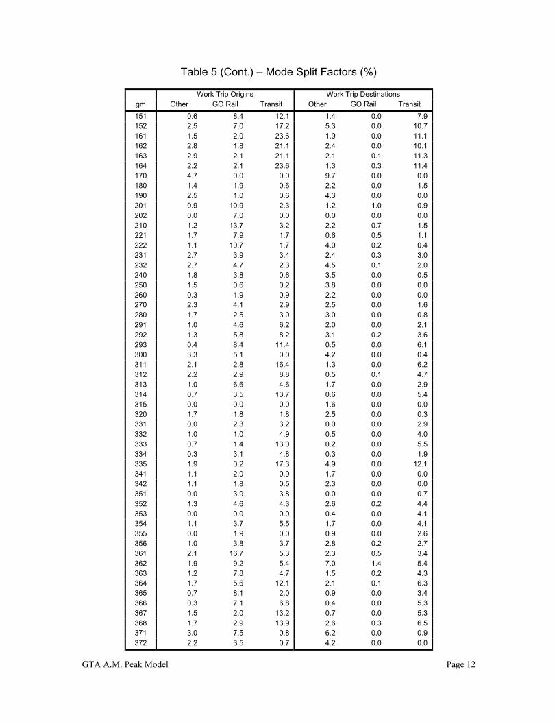
Table 5 – Mode Split Factors (%) ........................................................................................................ 11
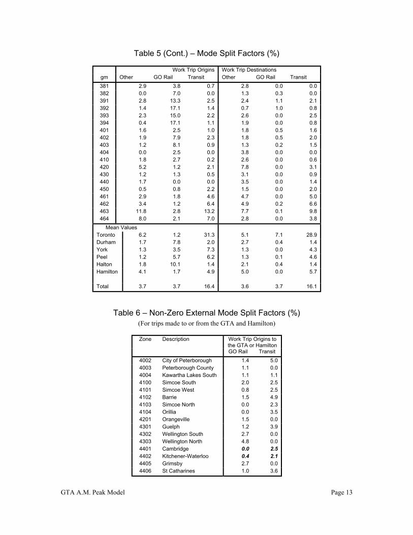
Table 6 – Non-Zero External Mode Split Factors (%) ......................................................................... 13
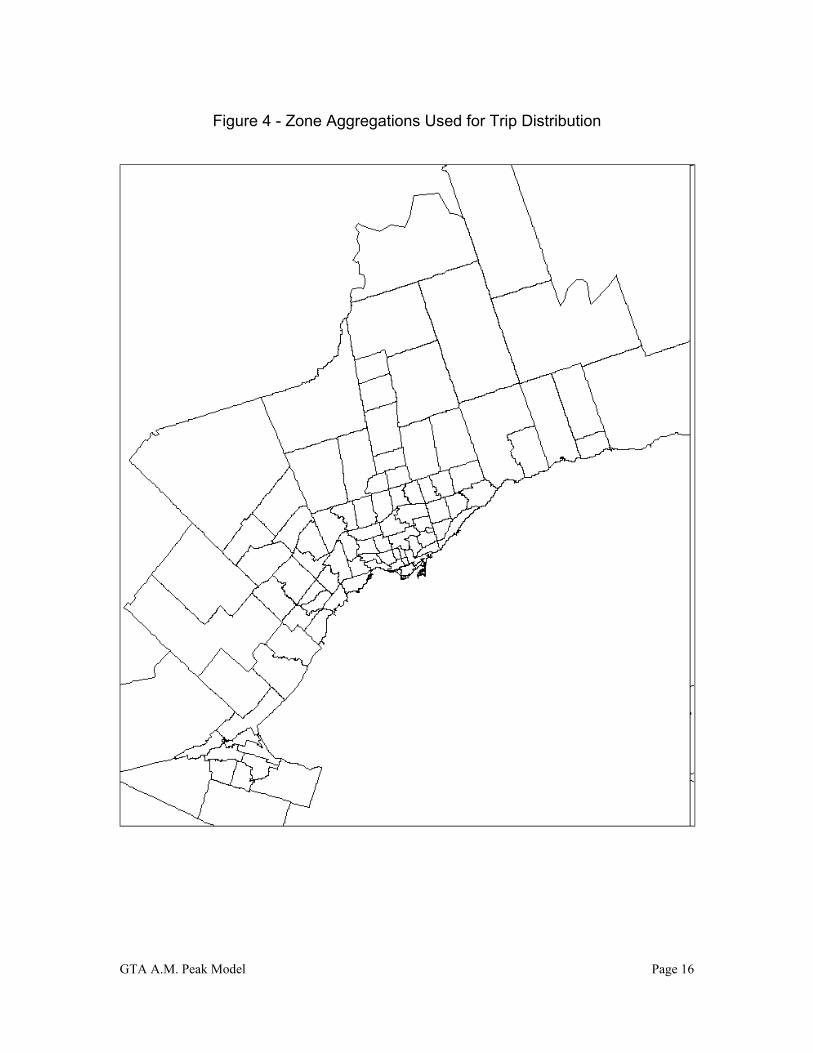
1.3 Trip Distribution........................................................................................................................... 14Figure 4 - Zone Aggregations Used for Trip Distribution.................................................................... 16
Table 7 – Calibration of Auto Trip Distribution................................................................................... 17
Table 8 - Trip Distribution Matrices..................................................................................................... 18
Table 9 – Validation of Trip Distribution............................................................................................. 18
1.4 Auto Assignment .......................................................................................................................... 18Table 10 - Auto Occupancy Factors – By Municipality (gp) or Zone Group (gg) ............................... 20
Table 11 - Auto Occupancy Factors – By Region ................................................................................ 21
Table 12 – Peak Hour Factors .............................................................................................................. 21
Figure 5 – Peak Hour Factor ................................................................................................................ 22
1.5 Transit Assignment....................................................................................................................... 222.0 Supplementary Features ................................................................................................................... 24
2.1 Trucking ....................................................................................................................................... 242.2 Trip Length Adjustment ............................................................................................................... 242.3 HOV Assignment ......................................................................................................................... 242.4 Zone Splitting ............................................................................................................................... 25
Table 13 - Population and Employment Weights for Zone Splitting ................................................... 25
3.0 Validation ......................................................................................................................................... 263.1 Land Use Data .............................................................................................................................. 26
Table 14 - Population Data by Region ................................................................................................. 26
Table 15 - Employed Labour Force by Region .................................................................................... 26
Table 16 - Employment by Region....................................................................................................... 27
3.2 Trip Generation, Mode Split and Distribution.............................................................................. 27Table 17 - Trip Totals and Travel Time Distributions within the GTA and Hamilton......................... 27
Table 18 – Municipal Self Containment of a.m. Peak Period Work Trips ........................................... 29
Table 19 – Municipal Self Containment of Auto Trips by Destination................................................ 30
3.3 Road assignment........................................................................................................................... 31Table 20 – Inter-Regional Screen Line Comparisons........................................................................... 31
Table 21 – City of Mississauga Screen Line Comparisons .................................................................. 32
3.4 Transit assignment........................................................................................................................ 33Table 22 – A.M. Peak Period Transit (GTA model – GO Rail included) ............................................ 33
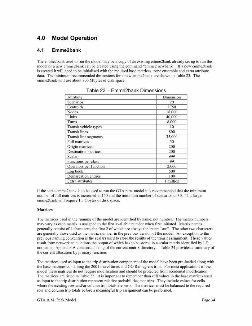
4.0 Model Operation............................................................................................................................... 344.1 Emme2bank.................................................................................................................................. 34
Table 23 – Emme2bank Dimensions.................................................................................................... 34
Table 24 - Matrix Allocation Table ...................................................................................................... 35
Table 25 – Base Matrices ..................................................................................................................... 35
Table 26 – Zone Ensembles.................................................................................................................. 35
Table 27 - Extra Attributes ................................................................................................................... 36
4.2 Macros .......................................................................................................................................... 36Table 28 - Macros................................................................................................................................. 37
4.3 Input Data ..................................................................................................................................... 38Table 29 - Recommended "Base Case" Input Parameter Values.......................................................... 39
4.4 Modification of Trip Generation Rates and Mode Split Factors .................................................. 394.5 Trip Distribution........................................................................................................................... 394.6 Auto Occupancy ........................................................................................................................... 404.7 Background Traffic (GO Rail Egress) .......................................................................................... 40
Table 30 - GO Rail Stations and Growth Factors................................................................................. 40
Table 31 - Subway Park and Ride ........................................................................................................ 41
4.8 Other Adjustment Factors............................................................................................................. 424.9 Model Outputs .............................................................................................................................. 42
Figure 6 - Aggregations Used for Output Summaries .......................................................................... 42
Appendix A - Emme/2 Matrix Directory...................................................................................................... 44Appendix B - Sample Printout of Performance Indicators ........................................................................... 47Appendix C – Trip Distribution Validation Plots......................................................................................... 50
GTA A.M. Peak Model Page 1
1.0 Introduction
The name “Simplified GTA model” has been adopted to distinguish between this model and the “Full GTAmodel” developed at the University of Toronto. The model is “simplified” in terms of its ease ofapplication. The level of detail, defined by the zone system and network information, is the same in bothmodels. The simplified GTA model has been used in a number of sub-area studies that involve the splittingof GTA zones for more detailed site specific analysis.
The simplified approach is based on the extrapolation of existing (observed) travel behaviour patterns asopposed to using mathematical equations to synthesize those relationships. Assumptions as to futurechanges in trip rates, mode choice factors, average trip length and auto occupancy have to be explicitlystated as inputs to the modelling process.
The model uses a pre-distribution (trip end) mode split component that favours the incorporation ofassumptions that reflect long term socio-economic trends, household decisions (such as car ownership) andgeneral, area wide, levels of service rather than the details of individual route planning.
The trip distribution component is unique to the simplified model incorporating features of both the moretraditional “gravity” and “Fratar” techniques. The results reflect both the existing O-D specific travelpatterns at an aggregate level as well as the existing trip length distribution at a more detailed level. Thelatter feature enables the trip distribution process to be applied to areas of new development for which thereis no existing travel information.
The trip generation, mode split and trip distribution components are based on a 3 hour peak period. Thetotal auto person trip matrix is converted to a peak hour auto driver matrix prior to assignment. The transitassignment, if required as an output, is for the 3 peak period. The model, in its most basic form, does notuse any network, or level of service information, to generate the trip matrices. Some of the supplementaryfeatures, discussed in Chapter 2, can be used to modify the trip distribution component to reflectanticipated changes in level of service.
The current release (version 4) has been calibrated using data from the 2001 Transportation TomorrowSurvey (TTS) and the 2001 Canada Census. To obtain complete coverage of the external areas the 2001TTS was supplemented by data from the 1996 TTS, for the Region of Waterloo and County ofNorthumberland, and by 1991 Census Place of work – Place of residence data for the Region ofHaldimand-Norfolk and the County of Brant. Model results have been validated using 2001 Cordon andtransit ridership counts. In addition a number of operational improvements have been made relative to theearlier versions.
There are currently three versions of the simplified model:1. An A.M. Peak period model for the entire GTA (Including Hamilton )2. A P.M. Peak period model for the entire GTA (Including Hamilton)3. A P.M. Peak period model developed specifically for the Regional Municipality of Halton.
This introduction is common to all 3 models.
The two GTA models are both based on the 1996 GTA zone system supplemented by 26 external zones.Some minor revisions, primarily re-calibration of the trip distribution component, will be necessary inorder to adapt the model to the 2001 GTA zone system. A refinement in the current release is the ability touse the same emme2bank to run both the A.M. and P.M. models with little or no risk of “interference”between the two models or accidental loss of results.
The Halton model covers the same geographic area as the GTA models but uses a more detailed zonesystem within the region of Halton. The same 26 external zones are used and the GTA zones are retainedin Peel Region and Parts of Hamilton. More aggregate zones are used in the rest of Hamilton, the City of
GTA
Toronto and in the Regions of Durham and York. The modelling procedures and the macros are identicalto those used in the GTA P.M. model.
1.1 Summary Description
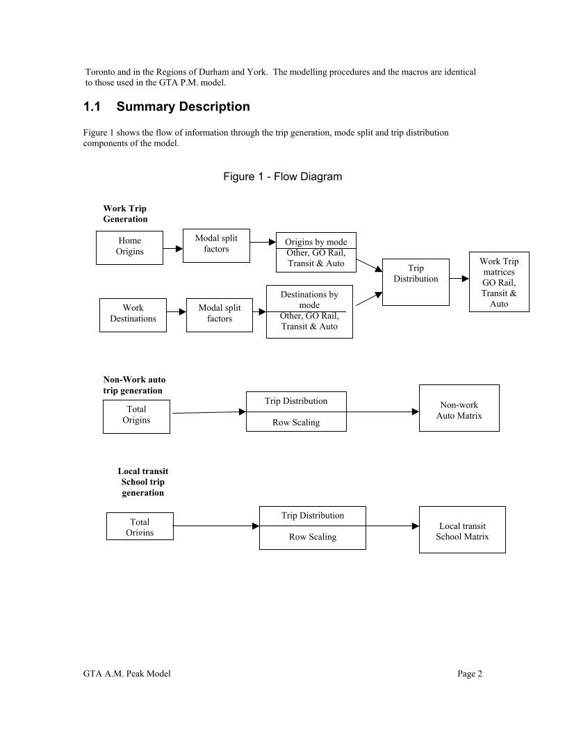
Figure 1 shows the flow of information through the trip generation, mode split and trip distributioncomponents of the model.
Figure 1 - Flow Diagram
Work TripGeneration
A.M. Peak Model
HomeOrigins
WorkDestinations
Modal splitfactors
Modal splitfactors
Non-Work autotrip generation
TotalOrigins
Trip
R
Local transitSchool tripgeneration
Origins by modeOther, GO Rail,Transit & Auto
TripDistribution
Destinations bymode
Other, GO Rail,Transit & Auto
Page
Distribution
ow Scaling
Non-worAuto Matr
Trip Distribution
Row ScalingLoca
Schoo
Work TripmatricesGO Rail,Transit &
Auto
kix
TotalOrigins
l transitl Matrix
2

GTA A.M. Peak Model Page 3
Table 1 provides a summary of the main features of the model. The model has been calibrated using the1996 TTS data
Table 1 - Features of the A.M. Peak Period Model
Time period a.m. peak 3 hrs (6:00 - 8:59)Geographic Scope GTA, including Hamilton-Wentworth, plus 10 adjacent
Counties and Regional MunicipalitiesZone system GTA96 plus 26 external zones (1703 total)Trip purpose categories 1. Work destinations (all modes)
2. Home to School (local transit only)3. Non work destinations (Auto only)
Modes 1. Auto (Driver & Passenger)2. Transit (Excluding GO Rail access)3. GO Rail4. Other, primarily walk & cycle (Trips not distributed
or assigned)Special Features 1. Bucket rounding used at all stages for the calculation
of trip end control totals and distributed cell values2. Modified auto trip distribution reflecting projected
changes in travel time (Optional).3. Simulation of HOV lanes including the formation of
new car-pools (Optional).4. Inclusion of an additional auto matrix that may be
used to represent GO Rail access, truck movementsor external and through trips from outside thesimulated area.
The definition of the GTA includes the Regional Municipality of Hamilton-Wentworth in the context of themodel and this documentation. The revised GTA model is compatible with the existing Durham regionsub-model that uses a more detailed zone system. It is anticipated that similar Regional sub-componentsmay be developed for other areas.
The model produces traffic assignments for auto drivers and local transit. In the trip generation and modesplit components the auto mode includes both auto passengers and auto drivers. A subsequent autooccupancy calculation is used to generate the auto driver matrix that is assigned. The mode-split componentincludes an "other" mode category (Primarily walk and cycle) but the trips are not distributed or assigned.
Bucket rounding is used, wherever applicable, to produce control totals and individual matrix cell valuesthat are integers. The bucket rounding function (bint) is described in full in section 3.7.2 of the emme/2User's Manual (Release 9). The advantages of using rounded integer values are:
a) Rounding errors are eliminated as a source of differences when data are exported from emme/2 forexternal analysis.
b) The size of the data files used to store, or transfer, matrix data is reduced dramatically due to thereduced number of non zero values and the absence of decimal places.
c) The standard output tables produced by emme/2 are more readable and easier to analyse.
A number of supplementary features may be used in conjunction with the basic model including adjustmentof the trip distribution to reflect changes in level of service and the analysis of HOV lanes. The full rangeof supplementary options is described in Chapter 2.
GTA A.M. Peak Model Page 4
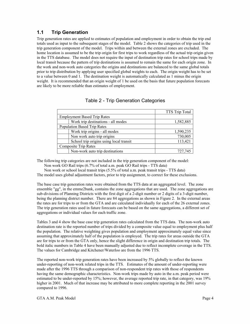
1.1 Trip GenerationTrip generation rates are applied to estimates of population and employment in order to obtain the trip endtotals used as input to the subsequent stages of the model. Table 2 shows the categories of trip used in thetrip generation component of the model. Trips within and between the external zones are excluded. Thehome location is assumed to be the trip origin for first trips to work regardless of the actual trip origin givenin the TTS database. The model does not require the input of destination trip rates for school trips made bylocal transit because the pattern of trip destinations is assumed to remain the same for each origin zone. Inthe work and non-work auto categories the origins and destinations are balanced to the same global totalsprior to trip distribution by applying user specified global weights to each. The origin weight has to be setto a value between 0 and 1. The destination weight is automatically calculated as 1 minus the originweight. It is recommended that an origin weight of 1 be used on the basis that future population forecastsare likely to be more reliable than estimates of employment.
Table 2 - Trip Generation Categories
TTS Trip TotalEmployment Based Trip Rates
Work trip destinations - all modes 1,582,885Population Based Trip Rates
Work trip origins - all modes 1,590,235Non work auto trip origins 730,005School trip origins using local transit 113,421
Composite Trip RatesNon-work auto trip destinations 727,745
The following trip categories are not included in the trip generation component of the model:Non work GO Rail trips (6.7% of total a.m. peak GO Rail trips - TTS data)Non work or school local transit trips (5.5% of total a.m. peak transit trips - TTS data)
The model uses global adjustment factors, prior to trip assignment, to correct for these exclusions.
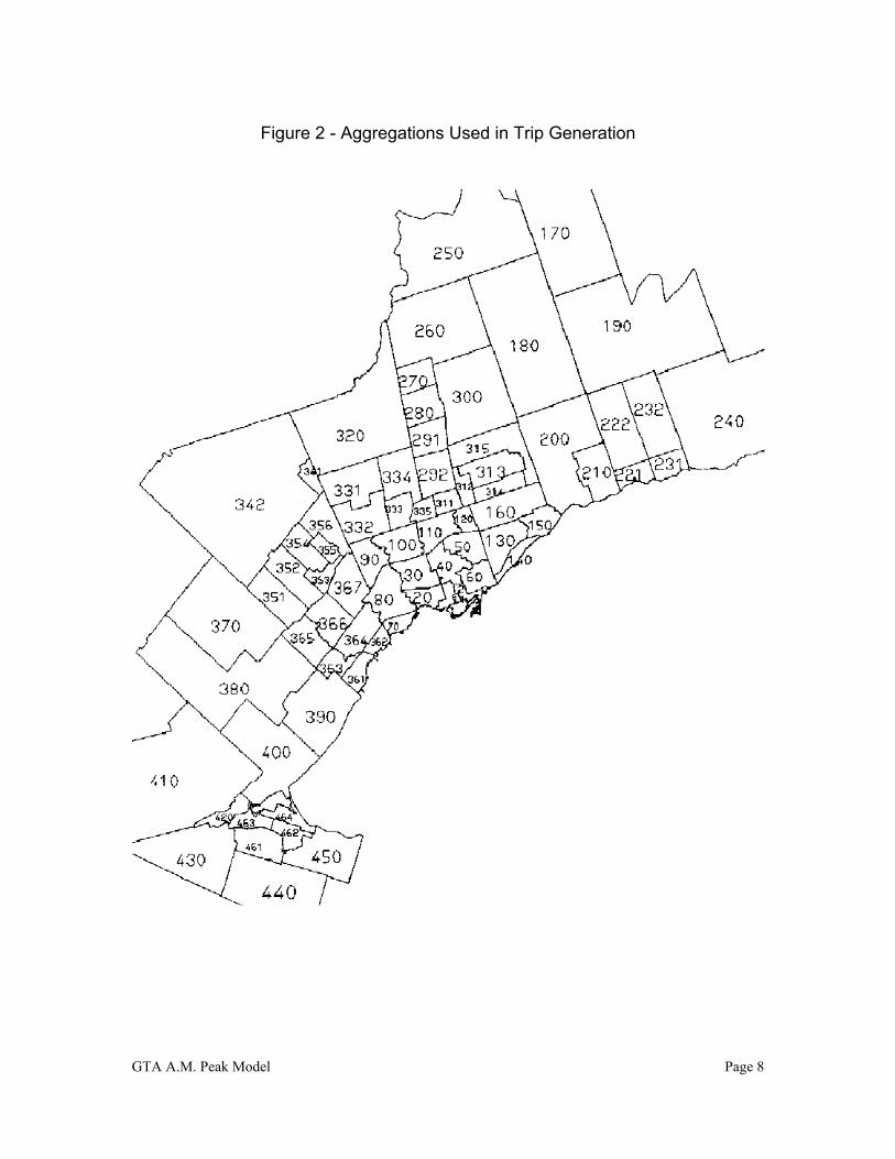
The base case trip generation rates were obtained from the TTS data at an aggregated level. The zoneensemble "gg", in the emme2bank, contains the zone aggregations that are used. The zone aggregations aresub-divisions of Planning Districts with the first digit of a 2-digit number or 2 digits of a 3-digit number,being the planning district number. There are 84 aggregations as shown in Figure 2. In the external areasthe rates are for trips to or from the GTA and are calculated individually for each of the 26 external zones.The trip generation rates used in future forecasts can be based on the same aggregations, a different set ofaggregations or individual values for each traffic zone.
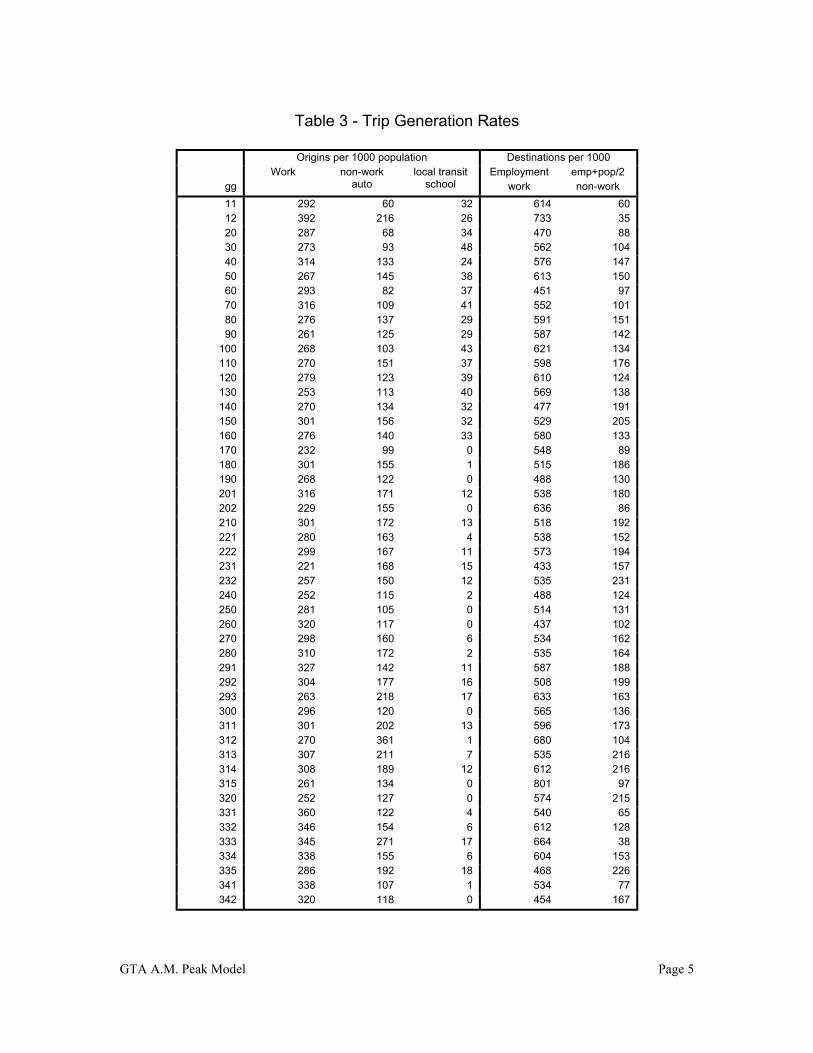
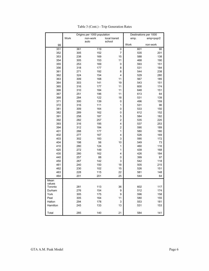
Tables 3 and 4 show the base case trip generation rates calculated from the TTS data. The non-work autodestination rate is the reported number of trips divided by a composite value equal to employment plus halfthe population. The relative weighting gives population and employment approximately equal value sinceassuming that approximately half of the population is employed. The trip rates for areas outside the GTAare for trips to or from the GTA only, hence the slight difference in origin and destination trip totals. Thebold italic numbers in Table 4 have been manually adjusted due to reflect incomplete coverage in the TTS.The values for Cambridge and Kitchener/Waterloo are from the 1996 TTS.
The reported non-work trip generation rates have been increased by 5% globally to reflect the knownunder-reporting of non-work related trips in the TTS. Estimates of the amount of under-reporting weremade after the 1996 TTS through a comparison of non-respondent trip rates with those of respondentshaving the same demographic characteristics. Non-work trips made by auto in the a.m. peak period wereestimated to be under-reported by 15%; however, the average reported trip rate, in that category, was 19%higher in 2001. Much of that increase may be attributed to more complete reporting in the 2001 surveycompared to 1996.
GTA A.M. Peak Model Page 5
Table 3 - Trip Generation Rates
Origins per 1000 population Destinations per 1000Employment emp+pop/2
ggWork non-work
autolocal transit
school work non-work
11 292 60 32 614 6012 392 216 26 733 3520 287 68 34 470 8830 273 93 48 562 10440 314 133 24 576 14750 267 145 38 613 15060 293 82 37 451 9770 316 109 41 552 10180 276 137 29 591 15190 261 125 29 587 142
100 268 103 43 621 134110 270 151 37 598 176120 279 123 39 610 124130 253 113 40 569 138140 270 134 32 477 191150 301 156 32 529 205160 276 140 33 580 133170 232 99 0 548 89180 301 155 1 515 186190 268 122 0 488 130201 316 171 12 538 180202 229 155 0 636 86210 301 172 13 518 192221 280 163 4 538 152222 299 167 11 573 194231 221 168 15 433 157232 257 150 12 535 231240 252 115 2 488 124250 281 105 0 514 131260 320 117 0 437 102270 298 160 6 534 162280 310 172 2 535 164291 327 142 11 587 188292 304 177 16 508 199293 263 218 17 633 163300 296 120 0 565 136311 301 202 13 596 173312 270 361 1 680 104313 307 211 7 535 216314 308 189 12 612 216315 261 134 0 801 97320 252 127 0 574 215331 360 122 4 540 65332 346 154 6 612 128333 345 271 17 664 38334 338 155 6 604 153335 286 192 18 468 226341 338 107 1 534 77342 320 118 0 454 167
GTA A.M. Peak Model Page 6
Table 3 (Cont.) - Trip Generation Rates
Origins per 1000 population Destinations per 1000Work non-work
autolocal transitschool
emp. emp+pop/2
gg Work non-work
351 361 119 0 601 90352 305 152 7 535 201353 238 169 15 588 138354 305 153 11 468 190355 253 169 0 593 151356 318 177 8 531 184361 271 192 8 544 238362 324 154 4 529 280363 309 168 11 567 185364 303 141 19 543 151365 316 177 11 600 174366 310 184 11 648 151367 251 196 11 613 64368 284 122 18 531 139371 300 139 0 496 159372 316 111 1 531 96381 309 164 0 533 150382 289 162 0 612 152391 258 187 5 584 182392 282 257 2 535 220393 316 195 4 537 253394 312 184 2 590 189401 288 177 1 580 180402 277 167 4 526 169403 302 183 3 590 172404 198 56 10 549 73410 280 124 1 460 116420 272 149 1 439 168430 280 162 4 426 184440 257 88 0 399 97450 267 142 3 542 118461 240 150 18 505 215462 230 102 15 526 151463 228 115 22 581 148464 201 201 25 544 64
MeanvaluesToronto 281 113 36 602 117Durham 276 154 9 512 174York 305 175 9 596 158Peel 305 164 11 580 155Halton 294 178 3 553 181Hamilton 245 133 13 531 153
Total 285 140 21 584 141
GTA A.M. Peak Model Page 7
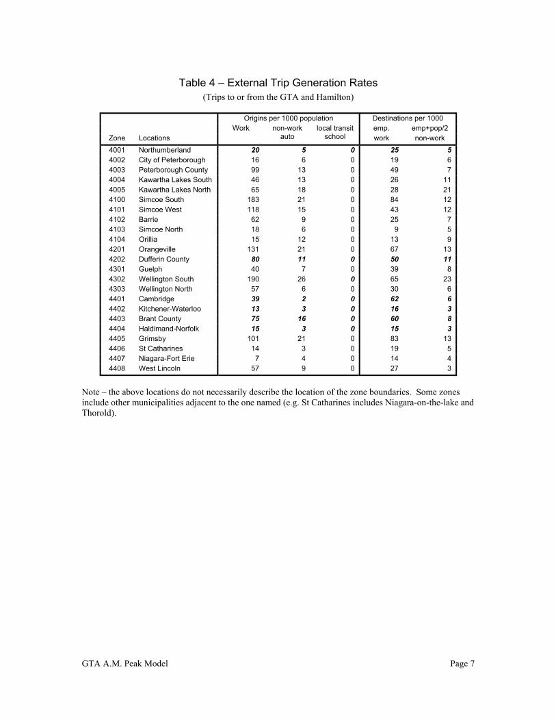
Table 4 – External Trip Generation Rates(Trips to or from the GTA and Hamilton)
Origins per 1000 population Destinations per 1000emp. emp+pop/2
Zone LocationsWork non-work
autolocal transit
school work non-work
4001 Northumberland 20 5 0 25 54002 City of Peterborough 16 6 0 19 64003 Peterborough County 99 13 0 49 74004 Kawartha Lakes South 46 13 0 26 114005 Kawartha Lakes North 65 18 0 28 214100 Simcoe South 183 21 0 84 124101 Simcoe West 118 15 0 43 124102 Barrie 62 9 0 25 74103 Simcoe North 18 6 0 9 54104 Orillia 15 12 0 13 94201 Orangeville 131 21 0 67 134202 Dufferin County 80 11 0 50 114301 Guelph 40 7 0 39 84302 Wellington South 190 26 0 65 234303 Wellington North 57 6 0 30 64401 Cambridge 39 2 0 62 64402 Kitchener-Waterloo 13 3 0 16 34403 Brant County 75 16 0 60 84404 Haldimand-Norfolk 15 3 0 15 34405 Grimsby 101 21 0 83 134406 St Catharines 14 3 0 19 54407 Niagara-Fort Erie 7 4 0 14 44408 West Lincoln 57 9 0 27 3
Note – the above locations do not necessarily describe the location of the zone boundaries. Some zonesinclude other municipalities adjacent to the one named (e.g. St Catharines includes Niagara-on-the-lake andThorold).
GTA A.M. Peak Model Page 8
Figure 2 - Aggregations Used in Trip Generation

GTA A.M. Peak Model Page 9
1.2 Mode Split
Mode split factors have to be supplied for both the origins and destinations of trips starting from work. Theorigins and destinations for each mode are factored to a common total, using a specified weighting factor,prior to calculation of the split for the next mode. The mode split factors applied in the running of themodel may be based on the same aggregations as used in the calibration, a different set of aggregations oron individual zone values.
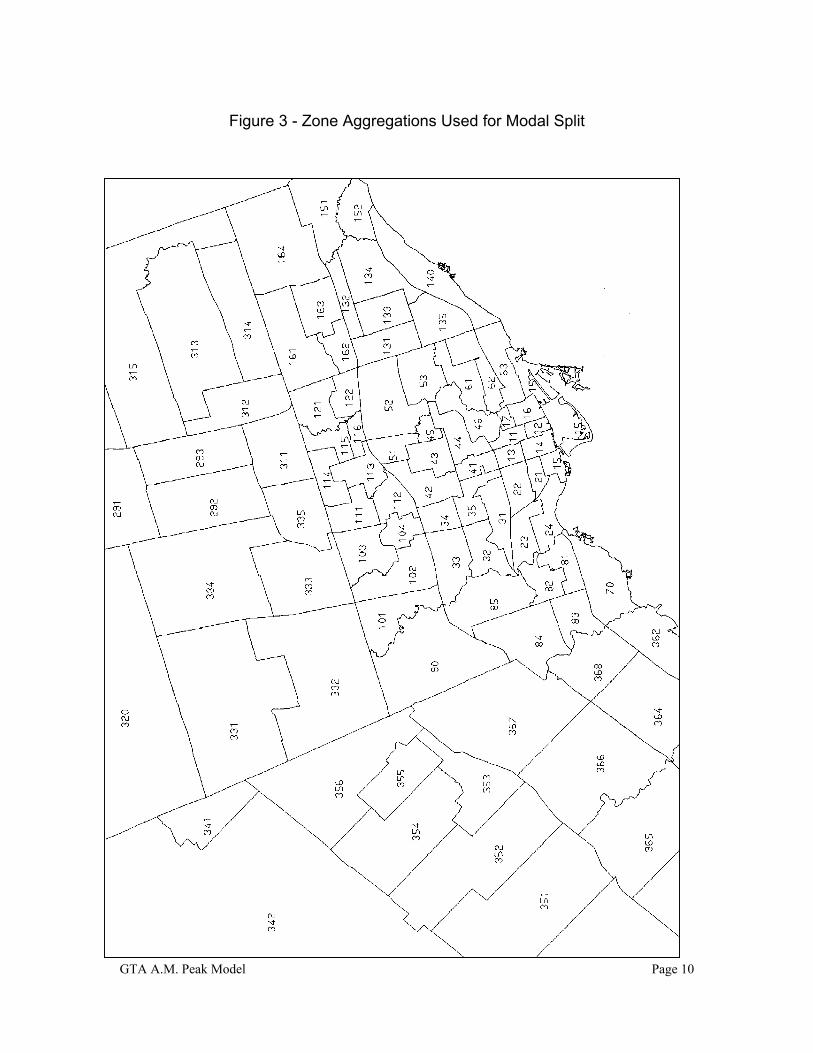
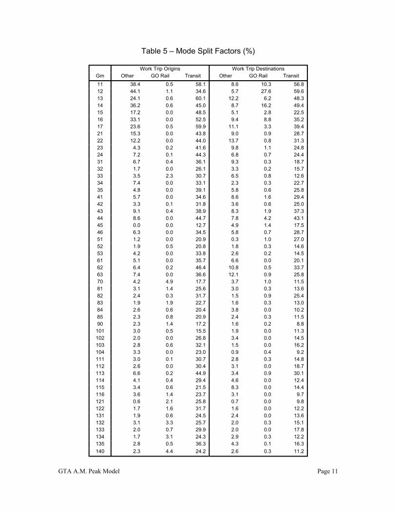
Figure 3 shows the zone aggregations used in the calibration of the mode split component of the model.The areas not shown have the same aggregations as are used for trip generation (Figure 2). Tables 5 and 6show the base case modal split factors calculated from TTS data. The zone aggregation ensemble "gm" isused. The numbering convention is the same as for the aggregations used in trip generation (i.e. the first 1or 2 digits are the planning district number). The total number of aggregations for the GTA and Hamiltonis 127. The external mode split factors shown in Table 6 apply to work trips made to or from the GTA andHamilton. Zones not shown in Table 6 are zero for both GO rail and local transit as are all the destinationvalues and the origin values for the other mode. The values for Cambridge and Kitchener-Waterloo arefrom the 1996 TTS.
The factors are applied sequentially to determine the subsequent mode shares after the previous mode hasbeen subtracted from the total. The sequence of application is
i) Other (Walk an Cycle)ii) GO Railiii) Local Transit
The remaining trips are assumed to be made by automobile (Driver or passenger).
The origins and destinations for each mode are scaled to a common total, using a user specified weightingfactor, prior to the calculation of the split for the next mode.
GTA A.M. Peak Model Page 10
Figure 3 - Zone Aggregations Used for Modal Split
GTA A.M. Peak Model Page 11
Table 5 – Mode Split Factors (%)
Work Trip Origins Work Trip DestinationsGm Other GO Rail Transit Other GO Rail Transit
11 38.4 0.5 58.1 8.6 10.3 56.812 44.1 1.1 34.6 5.7 27.6 59.613 24.1 0.6 60.1 12.2 6.2 48.314 36.2 0.6 45.0 8.7 16.2 49.415 17.2 0.0 48.5 5.1 2.8 22.516 33.1 0.0 52.5 9.4 8.8 35.217 23.6 0.5 59.9 11.1 3.3 39.421 15.3 0.0 43.8 9.0 0.9 28.722 12.2 0.0 44.0 13.7 0.8 31.323 4.3 0.2 41.6 9.8 1.1 24.824 7.2 0.1 44.3 6.8 0.7 24.431 6.7 0.4 36.1 9.3 0.3 18.732 1.7 0.0 26.1 3.3 0.2 15.733 3.5 2.3 30.7 6.5 0.8 12.634 7.4 0.0 33.1 2.3 0.3 22.735 4.8 0.0 39.1 5.8 0.6 25.841 5.7 0.0 34.6 8.6 1.6 29.442 3.3 0.1 31.8 3.6 0.6 25.043 9.1 0.4 38.9 8.3 1.9 37.344 8.6 0.0 44.7 7.8 4.2 43.145 0.0 0.0 12.7 4.9 1.4 17.546 6.3 0.0 34.5 5.8 0.7 28.751 1.2 0.0 20.9 0.3 1.0 27.052 1.9 0.5 20.8 1.8 0.3 14.653 4.2 0.0 33.8 2.6 0.2 14.561 5.1 0.0 35.7 6.6 0.0 20.162 6.4 0.2 46.4 10.8 0.5 33.763 7.4 0.0 36.6 12.1 0.9 25.870 4.2 4.9 17.7 3.7 1.0 11.581 3.1 1.4 25.6 3.0 0.3 13.682 2.4 0.3 31.7 1.5 0.9 25.483 1.9 1.9 22.7 1.6 0.3 13.084 2.6 0.6 20.4 3.8 0.0 10.285 2.3 0.8 20.9 2.4 0.3 11.590 2.3 1.4 17.2 1.6 0.2 8.8
101 3.0 0.5 15.5 1.9 0.0 11.3102 2.0 0.0 26.8 3.4 0.0 14.5103 2.8 0.6 32.1 1.5 0.0 16.2104 3.3 0.0 23.0 0.9 0.4 9.2111 3.0 0.1 30.7 2.8 0.3 14.8112 2.6 0.0 30.4 3.1 0.0 18.7113 6.6 0.2 44.9 3.4 0.9 30.1114 4.1 0.4 29.4 4.6 0.0 12.4115 3.4 0.6 21.5 8.3 0.0 14.4116 3.6 1.4 23.7 3.1 0.0 9.7121 0.6 2.1 25.8 0.7 0.0 9.8122 1.7 1.6 31.7 1.6 0.0 12.2131 1.9 0.6 24.5 2.4 0.0 13.6132 3.1 3.3 25.7 2.0 0.3 15.1133 2.0 0.7 29.9 2.0 0.0 17.8134 1.7 3.1 24.3 2.9 0.3 12.2135 2.8 0.5 36.3 4.3 0.1 16.3
140 2.3 4.4 24.2 2.6 0.3 11.2
GTA A.M. Peak Model Page 12
Table 5 (Cont.) – Mode Split Factors (%)
Work Trip Origins Work Trip Destinationsgm Other GO Rail Transit Other GO Rail Transit
151 0.6 8.4 12.1 1.4 0.0 7.9152 2.5 7.0 17.2 5.3 0.0 10.7161 1.5 2.0 23.6 1.9 0.0 11.1162 2.8 1.8 21.1 2.4 0.0 10.1163 2.9 2.1 21.1 2.1 0.1 11.3164 2.2 2.1 23.6 1.3 0.3 11.4170 4.7 0.0 0.0 9.7 0.0 0.0180 1.4 1.9 0.6 2.2 0.0 1.5190 2.5 1.0 0.6 4.3 0.0 0.0201 0.9 10.9 2.3 1.2 1.0 0.9202 0.0 7.0 0.0 0.0 0.0 0.0210 1.2 13.7 3.2 2.2 0.7 1.5221 1.7 7.9 1.7 0.6 0.5 1.1222 1.1 10.7 1.7 4.0 0.2 0.4231 2.7 3.9 3.4 2.4 0.3 3.0232 2.7 4.7 2.3 4.5 0.1 2.0240 1.8 3.8 0.6 3.5 0.0 0.5250 1.5 0.6 0.2 3.8 0.0 0.0260 0.3 1.9 0.9 2.2 0.0 0.0270 2.3 4.1 2.9 2.5 0.0 1.6280 1.7 2.5 3.0 3.0 0.0 0.8291 1.0 4.6 6.2 2.0 0.0 2.1292 1.3 5.8 8.2 3.1 0.2 3.6293 0.4 8.4 11.4 0.5 0.0 6.1300 3.3 5.1 0.0 4.2 0.0 0.4311 2.1 2.8 16.4 1.3 0.0 6.2312 2.2 2.9 8.8 0.5 0.1 4.7313 1.0 6.6 4.6 1.7 0.0 2.9314 0.7 3.5 13.7 0.6 0.0 5.4315 0.0 0.0 0.0 1.6 0.0 0.0320 1.7 1.8 1.8 2.5 0.0 0.3331 0.0 2.3 3.2 0.0 0.0 2.9332 1.0 1.0 4.9 0.5 0.0 4.0333 0.7 1.4 13.0 0.2 0.0 5.5334 0.3 3.1 4.8 0.3 0.0 1.9335 1.9 0.2 17.3 4.9 0.0 12.1341 1.1 2.0 0.9 1.7 0.0 0.0342 1.1 1.8 0.5 2.3 0.0 0.0351 0.0 3.9 3.8 0.0 0.0 0.7352 1.3 4.6 4.3 2.6 0.2 4.4353 0.0 0.0 0.0 0.4 0.0 4.1354 1.1 3.7 5.5 1.7 0.0 4.1355 0.0 1.9 0.0 0.9 0.0 2.6356 1.0 3.8 3.7 2.8 0.2 2.7361 2.1 16.7 5.3 2.3 0.5 3.4362 1.9 9.2 5.4 7.0 1.4 5.4363 1.2 7.8 4.7 1.5 0.2 4.3364 1.7 5.6 12.1 2.1 0.1 6.3365 0.7 8.1 2.0 0.9 0.0 3.4366 0.3 7.1 6.8 0.4 0.0 5.3367 1.5 2.0 13.2 0.7 0.0 5.3368 1.7 2.9 13.9 2.6 0.3 6.5371 3.0 7.5 0.8 6.2 0.0 0.9372 2.2 3.5 0.7 4.2 0.0 0.0
GTA A.M. Peak Model Page 13
Table 5 (Cont.) – Mode Split Factors (%)
Work Trip Origins Work Trip Destinationsgm Other GO Rail Transit Other GO Rail Transit
381 2.9 3.8 0.7 2.8 0.0 0.0382 0.0 7.0 0.0 1.3 0.3 0.0391 2.8 13.3 2.5 2.4 1.1 2.1392 1.4 17.1 1.4 0.7 1.0 0.8393 2.3 15.0 2.2 2.6 0.0 2.5394 0.4 17.1 1.1 1.9 0.0 0.8401 1.6 2.5 1.0 1.8 0.5 1.6402 1.9 7.9 2.3 1.8 0.5 2.0403 1.2 8.1 0.9 1.3 0.2 1.5404 0.0 2.5 0.0 3.8 0.0 0.0410 1.8 2.7 0.2 2.6 0.0 0.6420 5.2 1.2 2.1 7.8 0.0 3.1430 1.2 1.3 0.5 3.1 0.0 0.9440 1.7 0.0 0.0 3.5 0.0 1.4450 0.5 0.8 2.2 1.5 0.0 2.0461 2.9 1.8 4.6 4.7 0.0 5.0462 3.4 1.2 6.4 4.9 0.2 6.6463 11.8 2.8 13.2 7.7 0.1 9.8464 8.0 2.1 7.0 2.8 0.0 3.8
Mean ValuesToronto 6.2 1.2 31.3 5.1 7.1 28.9Durham 1.7 7.8 2.0 2.7 0.4 1.4York 1.3 3.5 7.3 1.3 0.0 4.3Peel 1.2 5.7 6.2 1.3 0.1 4.6Halton 1.8 10.1 1.4 2.1 0.4 1.4Hamilton 4.1 1.7 4.9 5.0 0.0 5.7
Total 3.7 3.7 16.4 3.6 3.7 16.1
Table 6 – Non-Zero External Mode Split Factors (%)(For trips made to or from the GTA and Hamilton)
Work Trip Origins tothe GTA or Hamilton
Zone Description
GO Rail Transit
4002 City of Peterborough 1.4 5.04003 Peterborough County 1.1 0.04004 Kawartha Lakes South 1.1 1.14100 Simcoe South 2.0 2.54101 Simcoe West 0.8 2.54102 Barrie 1.5 4.94103 Simcoe North 0.0 2.34104 Orillia 0.0 3.54201 Orangeville 1.5 0.04301 Guelph 1.2 3.94302 Wellington South 2.7 0.04303 Wellington North 4.8 0.04401 Cambridge 0.0 2.54402 Kitchener-Waterloo 0.4 2.14405 Grimsby 2.7 0.04406 St Catharines 1.0 3.6
GTA A.M. Peak Model Page 14
1.3 Trip Distribution
Trips to work are distributed by two-dimensional balancing of a "base" matrix to the desired origin anddestination zone totals for each of the three modes (auto, GO Rail and local transit). Non-work auto tripsare distributed in the same manner. School trips made by local transit are distributed by factoring each rowof the applicable "base" matrix to the desired row totals. The input "base" matrices are not trip matrices.They define an initial probability distribution that is comparable in its role to the impedance component ofa gravity model function. The matrices have been derived from the 2001 TTS data, supplemented by 1996TTS data for Waterloo and Northumberland and 1991 Census Place of Work – Place of Residence data forthe Regional municipality of Haldimand-Norfolk and the County of Brant. These “probability” matriceshave the following properties
a) When balanced to the TTS trip end totals they produce a trip pattern that is almost identical tothe TTS at an aggregated level (e.g.: PD to PD) but which is more uniformly distributed at theindividual zone level.
b) The observed TTS trip length distribution is closely maintained.c) The matrices for the auto mode have non-zero values in every row and column. The matrices
can therefore be used to obtain trip distributions in newly developed areas for which there isno existing trip data. The resulting trip length distribution should be similar to that observedin other areas. The GO Rail and transit matrices do have some zero row and column totals.These are in areas where there is currently no ridership at all even at a very aggregate level(e.g. Planning District).
Figure 4 shows the zone aggregations used in the calibration of the base trip distribution matrices. The firststep in that process was to aggregate the observed trip tables from the TTS database to these aggregations.The mean value of the zone to zone trip movements that make each aggregated group to group movementwas calculated by dividing the total trip movement by the total number of zone to zone pairs that make upthat aggregated block. For example if there were 5 zones in the zone group containing the origin zone and7 zones in the group containing the destination zone then the total number of trips between the origin groupand the destination group would be divided by 35 (5 x 7) to obtain the mean values. The mean value issubstituted in the observed matrix for all the zone pairs that make up the aggregation. In the case of GORail and local transit work trips the revised matrix is used as the base matrix for the distribution of thosetwo modes. The implied assumption is that the zones within each block have equally attractive with theresulting number of trips determined only by the relative magnitudes of the required origin and destinationtotals, i.e. the basics of a gravity model formulation.
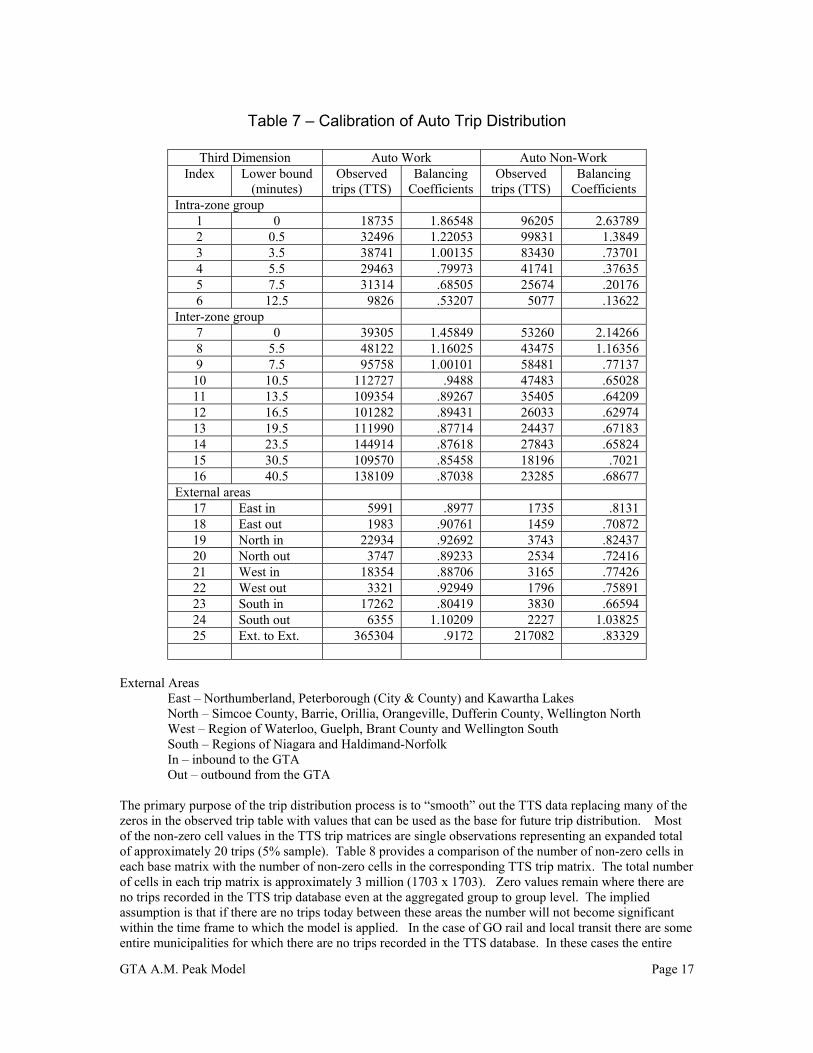
Using the mean value within each block does not work well for the auto trip distribution due primarily tothe much high propensity for very short trips to occur, either intra-zone or between adjacent zones. Thevalues in the base auto trip distribution matrices, both work and non-work, have been adjustment to moreaccurately reflect the actual trip length distribution. The method of adjustment uses the three-dimensionaltrip balancing feature available in emm/2. An index matrix, used as the third dimension, was created basedon the auto travel times between zones obtained from an equilibrium assignment of the 2001 TTS trip datato the 2001 road network. Separate index values were assigned to origin and destination cells within thesame zone group from those representing trip movements between different zone groups. Separate indexvalues were also used for trips to and from external areas. The number of observed (TTS) trips representedby each index value was recorded and used as the third dimension control totals in balancing the matrix ofmean values to the original TTS row and column trip totals by zone. The third dimension balancingcoefficients were saved and applied to the appropriate cells in the matrix of mean values to produce thefinal base matrix for each of the two trip purposes. The time intervals, trip totals and balancing coefficientsare shown in Table 7. The travel time intervals were selected to provide a reasonably uniform distributionof trip totals for each index value within the two categories – intra and inter zone group. There is littlevariation in the balancing coefficients for inter-group trips over 13.5 minutes in length. A single intervalwould likely have been sufficient. At the time the calibration of the trip distribution component was carriedout the model was structured to provide estimates of trip movements within and between external zones.

GTA A.M. Peak Model Page 15
The structure (trip rates) for external zones was subsequently changed to only include trips to/from theGTA and Hamilton. The external values (interval 25) in all the base matrices were changed to zero at thattime. Since the values in the matrices represent relative probabilities there was no need to change othervalues.
The base matrix for local transit school trips was obtained through the same process as was used for theauto trip distribution except that in addition to the third dimension balancing coefficients the columnbalancing coefficients were also applied in calculating the base matrix prior to normalizing the values ineach row to sum to a value of 1. At the current time the same base local transit school matrix is being usedas in the 1996 version of the model.
GTA A.M. Peak Model Page 16
Figure 4 - Zone Aggregations Used for Trip Distribution
GTA A.M. Peak Model Page 17
Table 7 – Calibration of Auto Trip Distribution
Third Dimension Auto Work Auto Non-WorkIndex Lower bound
(minutes)Observed
trips (TTS)Balancing
CoefficientsObserved
trips (TTS)Balancing
CoefficientsIntra-zone group
1 0 18735 1.86548 96205 2.637892 0.5 32496 1.22053 99831 1.38493 3.5 38741 1.00135 83430 .737014 5.5 29463 .79973 41741 .376355 7.5 31314 .68505 25674 .201766 12.5 9826 .53207 5077 .13622
Inter-zone group7 0 39305 1.45849 53260 2.142668 5.5 48122 1.16025 43475 1.163569 7.5 95758 1.00101 58481 .77137
10 10.5 112727 .9488 47483 .6502811 13.5 109354 .89267 35405 .6420912 16.5 101282 .89431 26033 .6297413 19.5 111990 .87714 24437 .6718314 23.5 144914 .87618 27843 .6582415 30.5 109570 .85458 18196 .702116 40.5 138109 .87038 23285 .68677
External areas17 East in 5991 .8977 1735 .813118 East out 1983 .90761 1459 .7087219 North in 22934 .92692 3743 .8243720 North out 3747 .89233 2534 .7241621 West in 18354 .88706 3165 .7742622 West out 3321 .92949 1796 .7589123 South in 17262 .80419 3830 .6659424 South out 6355 1.10209 2227 1.0382525 Ext. to Ext. 365304 .9172 217082 .83329
External AreasEast – Northumberland, Peterborough (City & County) and Kawartha LakesNorth – Simcoe County, Barrie, Orillia, Orangeville, Dufferin County, Wellington NorthWest – Region of Waterloo, Guelph, Brant County and Wellington SouthSouth – Regions of Niagara and Haldimand-NorfolkIn – inbound to the GTAOut – outbound from the GTA
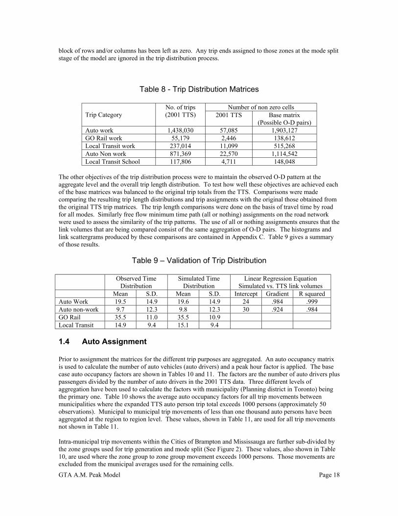
The primary purpose of the trip distribution process is to “smooth” out the TTS data replacing many of thezeros in the observed trip table with values that can be used as the base for future trip distribution. Mostof the non-zero cell values in the TTS trip matrices are single observations representing an expanded totalof approximately 20 trips (5% sample). Table 8 provides a comparison of the number of non-zero cells ineach base matrix with the number of non-zero cells in the corresponding TTS trip matrix. The total numberof cells in each trip matrix is approximately 3 million (1703 x 1703). Zero values remain where there areno trips recorded in the TTS trip database even at the aggregated group to group level. The impliedassumption is that if there are no trips today between these areas the number will not become significantwithin the time frame to which the model is applied. In the case of GO rail and local transit there are someentire municipalities for which there are no trips recorded in the TTS database. In these cases the entire
GTA A.M. Peak Model Page 18
block of rows and/or columns has been left as zero. Any trip ends assigned to those zones at the mode splitstage of the model are ignored in the trip distribution process.
Table 8 - Trip Distribution Matrices
Number of non zero cellsTrip Category
No. of trips(2001 TTS) 2001 TTS Base matrix
(Possible O-D pairs)Auto work 1,438,030 57,085 1,903,127GO Rail work 55,179 2,446 138,612Local Transit work 237,014 11,099 515,268Auto Non work 871,369 22,570 1,114,542Local Transit School 117,806 4,711 148,048
The other objectives of the trip distribution process were to maintain the observed O-D pattern at theaggregate level and the overall trip length distribution. To test how well these objectives are achieved eachof the base matrices was balanced to the original trip totals from the TTS. Comparisons were madecomparing the resulting trip length distributions and trip assignments with the original those obtained fromthe original TTS trip matrices. The trip length comparisons were done on the basis of travel time by roadfor all modes. Similarly free flow minimum time path (all or nothing) assignments on the road networkwere used to assess the similarity of the trip patterns. The use of all or nothing assignments ensures that thelink volumes that are being compared consist of the same aggregation of O-D pairs. The histograms andlink scattergrams produced by these comparisons are contained in Appendix C. Table 9 gives a summaryof those results.
Table 9 – Validation of Trip Distribution
Observed TimeDistribution
Simulated TimeDistribution
Linear Regression EquationSimulated vs. TTS link volumes
Mean S.D. Mean S.D. Intercept Gradient R squaredAuto Work 19.5 14.9 19.6 14.9 24 .984 .999Auto non-work 9.7 12.3 9.8 12.3 30 .924 .984GO Rail 35.5 11.0 35.5 10.9Local Transit 14.9 9.4 15.1 9.4
1.4 Auto Assignment
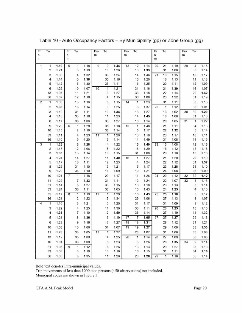
Prior to assignment the matrices for the different trip purposes are aggregated. An auto occupancy matrixis used to calculate the number of auto vehicles (auto drivers) and a peak hour factor is applied. The basecase auto occupancy factors are shown in Tables 10 and 11. The factors are the number of auto drivers pluspassengers divided by the number of auto drivers in the 2001 TTS data. Three different levels ofaggregation have been used to calculate the factors with municipality (Planning district in Toronto) beingthe primary one. Table 10 shows the average auto occupancy factors for all trip movements betweenmunicipalities where the expanded TTS auto person trip total exceeds 1000 persons (approximately 50observations). Municipal to municipal trip movements of less than one thousand auto persons have beenaggregated at the region to region level. These values, shown in Table 11, are used for all trip movementsnot shown in Table 11.
Intra-municipal trip movements within the Cities of Brampton and Mississauga are further sub-divided bythe zone groups used for trip generation and mode split (See Figure 2). These values, also shown in Table10, are used where the zone group to zone group movement exceeds 1000 persons. Those movements areexcluded from the municipal averages used for the remaining cells.

GTA A.M. Peak Model Page 19
In general it can be seen that average auto occupancy is lower for medium length trips than it is for eithershort trips or very long trips. Intra-municipal trips (values shown in bold type) generally have the highestlevel of auto occupancy. The TTS data does not include trip information for people under the age of 11 norare these included in the model. The average auto occupancy figures used in the model are therefore likelyto be lower than the values one would expect to observe on the street.
GTA A.M. Peak Model Page 20
Table 10 - Auto Occupancy Factors – By Municipality (gp) or Zone Group (gg)
From
To From
To From
To From
To From
To From
To
1 1 1.19 5 1 1.18 9 9 1.44 13 12 1.14 20 21 1.19 29 4 1.152 1.21 3 1.19 10 1.26 13 1.33 31 1.08 5 1.14
3 1.30 4 1.32 33 1.24 14 1.46 21 13 1.15 10 1.174 1.14 5 1.38 35 1.16 15 1.20 16 1.13 11 1.185 1.12 6 1.30 36 1.11 16 1.25 20 1.11 12 1.09
6 1.22 10 1.07 10 1 1.21 31 1.16 21 1.39 16 1.0713 1.07 11 1.21 3 1.27 33 1.18 22 1.14 29 1.4236 1.07 12 1.18 4 1.15 36 1.08 23 1.22 31 1.19
2 1 1.30 13 1.16 8 1.15 14 1 1.23 31 1.11 33 1.15
2 1.33 16 1.14 9 1.25 6 1.37 22 1 1.12 36 1.01
3 1.19 31 1.11 10 1.34 13 1.27 13 1.02 30 30 1.204 1.10 33 1.18 11 1.23 14 1.45 16 1.08 31 1.10
8 1.17 36 1.06 33 1.27 16 1.14 20 1.05 31 1 1.22
9 1.20 6 1 1.28 35 1.18 15 1 1.48 21 1.11 4 1.1310 1.15 2 1.19 36 1.14 5 1.17 22 1.32 5 1.14
33 1.11 4 1.23 11 1 1.20 13 1.19 23 1.17 10 1.1136 1.10 5 1.20 3 1.14 14 1.49 31 1.08 11 1.15
3 1 1.28 6 1.28 4 1.22 15 1.49 23 13 1.08 12 1.162 1.47 12 1.06 5 1.22 16 1.29 16 1.12 13 1.163 1.35 13 1.14 10 1.15 31 1.08 20 1.10 16 1.16
4 1.24 14 1.27 11 1.40 16 1 1.27 21 1.20 29 1.105 1.17 16 1.11 12 1.23 4 1.24 22 1.12 31 1.378 1.25 31 1.10 13 1.21 5 1.17 23 1.28 33 1.109 1.20 36 1.10 16 1.09 10 1.21 24 1.08 36 1.09
10 1.21 7 1 1.18 29 1.17 11 1.26 24 20 1.12 32 32 1.12
11 1.22 7 1.33 31 1.11 12 1.24 22 1.07 33 1 1.1631 1.14 8 1.27 33 1.15 13 1.18 23 1.13 3 1.1433 1.24 36 1.11 36 1.05 15 1.43 24 1.25 4 1.16
35 1.17 8 1 1.19 12 1 1.29 16 1.43 25 25 1.18 5 1.1736 1.21 2 1.22 5 1.34 29 1.06 27 1.13 8 1.07
4 1 1.16 3 1.21 10 1.25 31 1.17 31 1.09 9 1.12
3 1.22 4 1.25 11 1.30 33 1.11 26 26 1.25 10 1.164 1.33 7 1.10 12 1.50 36 1.14 27 1.19 11 1.32
5 1.21 8 1.36 13 1.19 17 17 1.05 27 27 1.27 29 1.13
6 1.23 9 1.16 16 1.27 18 18 1.31 28 1.12 31 1.21
10 1.08 10 1.06 31 1.07 19 19 1.27 29 1.08 33 1.30
11 1.28 33 1.05 13 1 1.27 23 1.07 31 1.06 35 1.08
13 1.12 35 1.09 4 1.25 20 1 1.14 28 27 1.09 36 1.05
16 1.01 36 1.08 5 1.23 5 1.26 28 1.35 34 9 1.14
31 1.05 9 1 1.12 6 1.26 13 1.13 29 1.27 33 1.1033 1.08 3 1.19 10 1.16 16 1.15 31 1.11 34 1.16
36 1.08 8 1.35 11 1.28 20 1.28 29 1 1.16 35 1.14
Bold text denotes intra-municipal values.Trip movements of less than 1000 auto persons (~50 observations) not included.Municipal codes are shown in Figure 3.
GTA A.M. Peak Model Page 21
Table 10 (Cont.) - Auto Occupancy Factors by Municipality or Zone Group (gg)
From
To From
To From
To From To From
To From
To
34 36 1.07 36 8 1.11 38 39 1.11 43 43 1.35 Peel sub-areas (gg)
35 1 1.18 9 1.14 39 1 1.15 46 1.13 352 363 1.24 364 360 1.38
3 1.08 10 1.08 8 1.15 44 46 1.15 354 353 1.26 362 1.25
4 1.29 11 1.06 35 1.07 45 40 1.08 354 1.43 363 1.168 1.09 13 1.15 36 1.09 45 1.27 355 1.46 364 1.39
9 1.18 16 1.12 39 1.29 46 1.16 356 1.28 365 359 1.20
10 1.17 31 1.05 40 1.12 46 36 1.09 363 1.16 360 1.17
11 1.30 33 1.08 46 1.05 39 1.11 356 352 1.46 361 1.37
33 1.11 35 1.12 40 1 1.12 40 1.11 353 1.19 362 1.1534 1.50 36 1.21 36 1.06 41 1.25 354 1.29 363 1.09
35 1.15 38 1.11 38 1.08 42 1.13 356 1.39 366 360 1.2136 1.10 39 1.15 39 1.10 43 1.18 363 1.19 361 1.25
39 1.15 40 1.05 40 1.30 45 1.16 361 357 1.47 362 1.42
36 1 1.16 37 35 1.13 46 1.08 46 1.27 362 358 1.41 363 1.16
2 1.13 36 1.07 41 40 1.15 Peel sub-areas (gg) 363 359 1.44 367 363 1.29
3 1.12 37 1.23 41 1.19 352 352 1.44 360 1.15 368 363 1.314 1.17 38 1.18 46 1.16 353 1.57 361 1.09 364 1.38
5 1.12 38 36 1.11 42 42 1.33 356 1.13 363 1.07
7 1.11 38 1.23 46 1.12 362 1.06
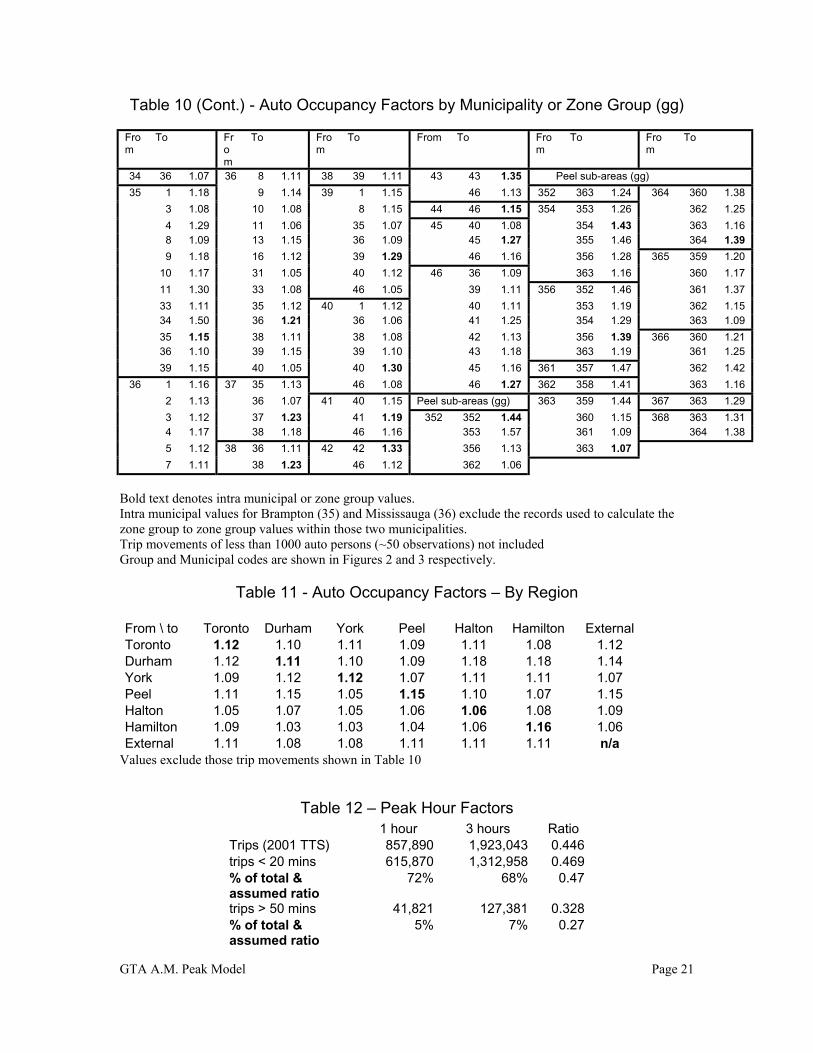
Bold text denotes intra municipal or zone group values.Intra municipal values for Brampton (35) and Mississauga (36) exclude the records used to calculate thezone group to zone group values within those two municipalities.Trip movements of less than 1000 auto persons (~50 observations) not includedGroup and Municipal codes are shown in Figures 2 and 3 respectively.
Table 11 - Auto Occupancy Factors – By Region
From \ to Toronto Durham York Peel Halton Hamilton ExternalToronto 1.12 1.10 1.11 1.09 1.11 1.08 1.12Durham 1.12 1.11 1.10 1.09 1.18 1.18 1.14York 1.09 1.12 1.12 1.07 1.11 1.11 1.07Peel 1.11 1.15 1.05 1.15 1.10 1.07 1.15Halton 1.05 1.07 1.05 1.06 1.06 1.08 1.09Hamilton 1.09 1.03 1.03 1.04 1.06 1.16 1.06External 1.11 1.08 1.08 1.11 1.11 1.11 n/a
Values exclude those trip movements shown in Table 10
Table 12 – Peak Hour Factors1 hour 3 hours Ratio
Trips (2001 TTS) 857,890 1,923,043 0.446trips < 20 mins 615,870 1,312,958 0.469% of total &assumed ratio
72% 68% 0.47
trips > 50 mins 41,821 127,381 0.328% of total &assumed ratio
5% 7% 0.27
GTA A.M. Peak Model Page 22
Figure 5 – Peak Hour Factor
0.100
0.150
0.200
0.250
0.300
0.350
0.400
0.450
0.500
0.550
0 5 10 15 20 25 30 35 40 45 50 55 60 65 70 75 80 85 90 95
Trip Length (minutes)
Rat
io -
1 h
ou
r to
3 h
ou
rs
TTS data
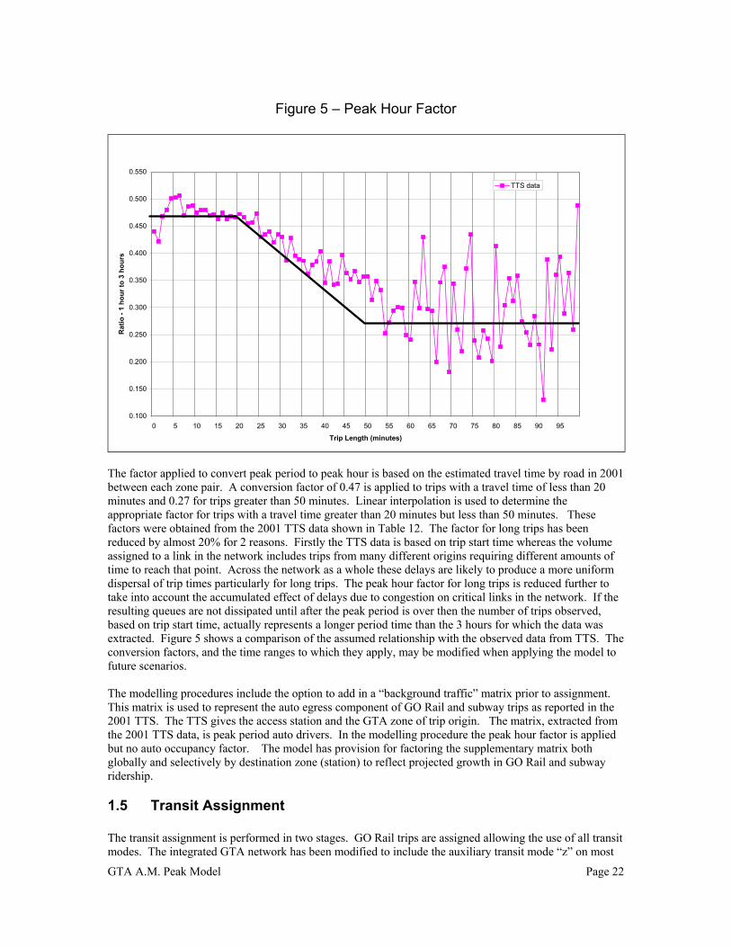
The factor applied to convert peak period to peak hour is based on the estimated travel time by road in 2001between each zone pair. A conversion factor of 0.47 is applied to trips with a travel time of less than 20minutes and 0.27 for trips greater than 50 minutes. Linear interpolation is used to determine theappropriate factor for trips with a travel time greater than 20 minutes but less than 50 minutes. Thesefactors were obtained from the 2001 TTS data shown in Table 12. The factor for long trips has beenreduced by almost 20% for 2 reasons. Firstly the TTS data is based on trip start time whereas the volumeassigned to a link in the network includes trips from many different origins requiring different amounts oftime to reach that point. Across the network as a whole these delays are likely to produce a more uniformdispersal of trip times particularly for long trips. The peak hour factor for long trips is reduced further totake into account the accumulated effect of delays due to congestion on critical links in the network. If theresulting queues are not dissipated until after the peak period is over then the number of trips observed,based on trip start time, actually represents a longer period time than the 3 hours for which the data wasextracted. Figure 5 shows a comparison of the assumed relationship with the observed data from TTS. Theconversion factors, and the time ranges to which they apply, may be modified when applying the model tofuture scenarios.
The modelling procedures include the option to add in a “background traffic” matrix prior to assignment.This matrix is used to represent the auto egress component of GO Rail and subway trips as reported in the2001 TTS. The TTS gives the access station and the GTA zone of trip origin. The matrix, extracted fromthe 2001 TTS data, is peak period auto drivers. In the modelling procedure the peak hour factor is appliedbut no auto occupancy factor. The model has provision for factoring the supplementary matrix bothglobally and selectively by destination zone (station) to reflect projected growth in GO Rail and subwayridership.
1.5 Transit Assignment
The transit assignment is performed in two stages. GO Rail trips are assigned allowing the use of all transitmodes. The integrated GTA network has been modified to include the auxiliary transit mode “z” on most

GTA A.M. Peak Model Page 23
road links outside the City of Toronto with a fixed operating speed of 40 kph. Mode “z” is used torepresent the auto access component of GO Rail trips. The assignment procedure does not "force" trips onto GO Rail if the network provides a more attractive alternative using local transit. The assigned GO Railvolumes may therefore be slightly less than the volumes obtained from the mode split calculations. GORail volumes can also be obtained by aggregating the trip matrix to station catchment area (ensemble gs).These volumes will be consistent with the mode-split calculations.
Local transit trips are assigned without permitting the use of modes “r” or “z” (GO Rail and GO Railaccess). The resulting transit assignment does not include the use of local transit to provide access oregress to GO Rail stations, other than in the City of Toronto, unless local transit provides for a fasteralternative than mode “z” (highly unlikely).
A transit network is not needed for Trip Generation, Mode Split and Trip Distribution. The model can beused to analyse future transit demand on an existing network without the need for detailed specification offuture service levels on every route. The scenario used for the transit assignment is specified separatelyfrom the scenario used for the road assignment. A single integrated network can be used for bothassignments or two separate networks can be used. The latter is strongly recommended for mostapplications.
The transit assignment macro contains the following values for the parameters that have to be specified inorder to perform a transit assignment. The same values are used for both the GO rail and local transitcomponents.
Source for effective headways = actual line headways with maximum (option 2)Maximum effective headway = 15Source for boarding times = same value for entire network (option 1)Boarding time = 2Source for wait time factors = same value for entire network (option 1)Wait time factor = 0.5Wait time weight = 2Auxiliary transit time weight = 1Boarding time weight = 1
Changing the above values is unlikely to have any significant effect on the assigned volumes but willchange the computed travel costs. The transit travel cost (equivalent time) matrix is not saved as a standardoutput.
GTA A.M. Peak Model Page 24
2.0 Supplementary Features
The following features are not part of the basic model but are either available, as supplementary macros, orcan be easily incorporated. Some have already been built into current Halton Region model applications.
2.1 Trucking
The basic modelling and assignment procedures do not include trucks. If total link volumes, includingtrucks, is required as an output the recommended procedure is to apply appropriate adjustment factors tothe assigned auto volumes. A network calculation can be performed to apply different factors by link type,vdf number or any other link attribute. Alternatively appropriate factors, calibrated on the basis of cordonand other count data, can be stored as an extra attribute and applied more selectively. The latter approachhas been used with the Halton Region P.M. peak model.
2.2 Trip Length Adjustment
Trip distribution in the basic model is an extrapolation of existing travel patterns without consideration ofimprovements in the network or other changes in level of service that might occur in the future. The triplength adjustment procedure allows such changes to be taken into account. The home to work auto tripdistribution is modified to reflect projected changes in travel between zones based on the equilibriumassignment of the initial trip table produced by the model. The simulated travel times for single occupantvehicles from the initial trip distribution are compared with the base year (2001) travel times. An elasticityfactor is applied to increase, or decrease, the "impedance" value for each cell in the base matrix used asinput to the trip end balancing procedure. The result of the adjustment is to increase the number of tripsbetween origins and destinations where there is a projected improvement in travel time and to decrease thenumber trips between zones where there is a projected increase in travel time. The sensitivity of theadjustment is controlled by a coefficient the default value of which (0.03) has been set based on experiencewith the a.m. Peak model. The default value will produce a trip length distribution that lies approximatelymidway between one having the same mean trip length (km) and one having the same mean travel time asthe observed 2001 trip distribution.
2.3 HOV AssignmentThe model includes routines to perform an HOV assignment and to estimate the number of new HOVs thatmight be formed as a result of potential time savings. Both routines require a road network that has eachHOV lane coded as a separate series of nodes and links from the general use lanes. General use linksrequire the mode codes "i" and "j" in addition to the mode code "c". Links restricted to vehicles with twoor more occupants require the mode code "i" in addition to the mode code "c". Mode code "c" should bethe only auto mode on links restricted to vehicles with 3 more occupants.
The first step in the HOV assignment procedure is to stratify the total auto vehicle matrix into 3 matricesrepresenting 1 occupant, 2 occupant and 3 plus occupant vehicles. The stratification formulae are:
P2 = 1.01(1- x)P3 = 0.16(1 - x)
Wherex = mean auto occupancy used to convert auto person trips to auto vehicles (Table 6).P2 is the proportion of automobiles with two occupantsP3 is the proportion of automobiles with three or more occupants.
The coefficients have been calibrated to provide a distribution that matches the auto occupancy distributionobserved across selected screen lines in the GTA. The observed distribution was obtained from availableCordon Count data. The implied auto occupancy, calculated from the distribution, will be higher than that
GTA A.M. Peak Model Page 25
shown in Table 6 since the calibration takes into account persons under the age of 11 who are not includedin other components of the model. The coefficients may be modified if desired and are different from therecommended values for use in the p.m. peak period (0.85 and 0.1).
A multiclass assignment is used to calculate link volumes and travel time matrices for each of the threecategories of vehicle (1 person, 2 persons and 3 plus persons). A second procedure estimates the number ofnew HOVs that might be formed as a result of differences in travel time between the three categories. Twofactors are used to calculate the diversion. The first is the proportion of the occupants of single personvehicles that will get together to form two person “car pools” for each minute of time saving that there isbetween one and two person vehicles. The second factor is the proportion of one and two person vehicleoccupants that will combine to form three person “car pools” for each additional minute of time savingbetween two and three person vehicles. The procedure has been tested using values of 0.02 and 0.01respectively for these two factors reflecting the observed experience when carpool lanes were firstintroduced on the Shirley highway in Washington D.C. The factors may be modified to reflect localexperience. A second multiclass assignment completes is performed to complete the procedure.
2.4 Zone Splitting
Zone splitting can be used to increase the level of network detail and assignment results for a specific sub-area. The procedure to do that is to run the model using the existing zone system for which the model hasbeen calibrated. The trips contained in the resulting auto driver trip table are then re-distributed betweenthe sub-zones that make up each of the original zones on the basis of population and employment. A macrois available to perform the re-distribution using the weights shown in Table 13. These weights have beencalculated on the basis of average trip generation rates and combination of trip purposes. The populationand employment numbers assigned to the sub-zones are used to determine the proportion of trips to beassigned to each sub-zone. The total number of trips remains the same even if the total population oremployment differs from the zone total used to run the model.
Table 13 - Population and Employment Weights for Zone Splitting
Employment Weight Population weightOrigins Destinations Origins Destinations
a.m. model 0.05 0.9 0.95 0.1p.m. model 0.8 0.35 0.2 0.65
The zone splitting procedure can be applied within the same emme2bank as was used to run the modelproviding that the following rules are followed in assigning numbers to the sub-zones.
1. The original zone numbers are retained, either as one of the sub-zone numbers or as dummyzones with zero population and employment.
2. Any new zone numbers that are assigned must have a zone number higher than that of anyexisting zone.
Failure to adhere to the above rules will cause corruption of the matrix data already contained in theemme2bank.
GTA A.M. Peak Model Page 26
3.0 ValidationValidation of the model consists primarily of comparisons between a 2001 "Base Case" simulation, the2001 TTS data and available cordon count information. The network used in the calibration of the modelwas Release 1 of the 2001 integrated network developed at the DMG. The same network, with minormodifications made by City of Mississauga staff, was used in the validation.
3.1 Land Use Data
The trip generation rates and mode split factors have been calculated using the population and employmentdata contained in the 1996 TTS database. The base case simulation (2001aa) uses a combination ofpopulation from the census and employment data from the TTS. The total GTA population reported in theTTS is 3.3% lower than that given by the census. The TTS is known to under represent infants, under theage of 1, and seniors, over the age of 75, many of whom live in collective homes not included in the survey.Since neither of these two categories of people is likely to make any significant number of trips the TTStrip rates will be artificially high when applied to the total population. No adjustment has been made to thetrip rates but a global adjustment factor of .97 is recommended when applying the trip rates to populationestimates based on census data.
Table 14 - Population Data by Region
2001 TTS 2001 Census Base Case (2001aa)Toronto 2,368,717 2,476,177 2,476,178
Durham 492,197 506,901 506,897
York 720,954 729,254 729,245
Peel 954,231 988,948 988,947
Halton 364,107 375,229 375,229
Hamilton 485,957 490,268 490,275
Total GTA 5,386,163 5,566,777 5,566,771
Employed Labour Force is not calculated or used directly in the model but is clearly a factor in determiningtrip generation rates. Table 15 compares the TTS and Census data. The Census and TTS occurred atdifferent times of the year, which may account for some of the differences. There may also be somedifference due to definition, for example the census includes people who worked the previous week butwho were not actually employed on the day of the census. No adjustments to trip rates have been made orare recommended at this time.
Table 15 - Employed Labour Force by Region
2001 TTS 2001 Census Difference
Toronto 1,192,866 1,228,015 -35,149 -2.9%Durham 253,498 247,395 6,103 2.5%York 379,915 387,620 -7,705 -2.0%Peel 507,829 535,330 -27,501 -5.1%Halton 188,799 204,600 -15,801 -7.7%Hamilton 230,543 232,240 -1,697 -0.7%Total GTA 2,753,450 2,835,200 -81,750 -2.9%
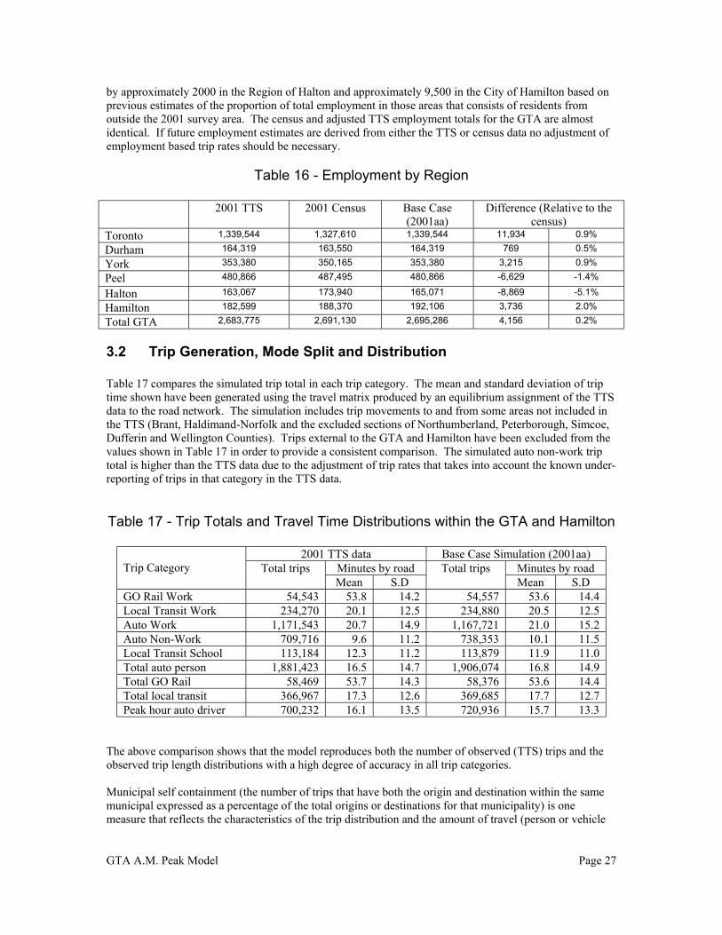
Table 16 provides a comparison of employment data. The same comments, with respect to timing anddefinitions, apply as for the employed labour force. In addition the TTS employment figures do not includeworkers who live outside the TTS area. Scaling factors have been applied to increase the total employment
GTA A.M. Peak Model Page 27
by approximately 2000 in the Region of Halton and approximately 9,500 in the City of Hamilton based onprevious estimates of the proportion of total employment in those areas that consists of residents fromoutside the 2001 survey area. The census and adjusted TTS employment totals for the GTA are almostidentical. If future employment estimates are derived from either the TTS or census data no adjustment ofemployment based trip rates should be necessary.
Table 16 - Employment by Region
2001 TTS 2001 Census Base Case(2001aa)
Difference (Relative to thecensus)
Toronto 1,339,544 1,327,610 1,339,544 11,934 0.9%
Durham 164,319 163,550 164,319 769 0.5%
York 353,380 350,165 353,380 3,215 0.9%
Peel 480,866 487,495 480,866 -6,629 -1.4%
Halton 163,067 173,940 165,071 -8,869 -5.1%
Hamilton 182,599 188,370 192,106 3,736 2.0%
Total GTA 2,683,775 2,691,130 2,695,286 4,156 0.2%
3.2 Trip Generation, Mode Split and Distribution
Table 17 compares the simulated trip total in each trip category. The mean and standard deviation of triptime shown have been generated using the travel matrix produced by an equilibrium assignment of the TTSdata to the road network. The simulation includes trip movements to and from some areas not included inthe TTS (Brant, Haldimand-Norfolk and the excluded sections of Northumberland, Peterborough, Simcoe,Dufferin and Wellington Counties). Trips external to the GTA and Hamilton have been excluded from thevalues shown in Table 17 in order to provide a consistent comparison. The simulated auto non-work triptotal is higher than the TTS data due to the adjustment of trip rates that takes into account the known under-reporting of trips in that category in the TTS data.
Table 17 - Trip Totals and Travel Time Distributions within the GTA and Hamilton
2001 TTS data Base Case Simulation (2001aa)Minutes by road Minutes by roadTrip Category Total tripsMean S.D
Total tripsMean S.D
GO Rail Work 54,543 53.8 14.2 54,557 53.6 14.4Local Transit Work 234,270 20.1 12.5 234,880 20.5 12.5Auto Work 1,171,543 20.7 14.9 1,167,721 21.0 15.2Auto Non-Work 709,716 9.6 11.2 738,353 10.1 11.5Local Transit School 113,184 12.3 11.2 113,879 11.9 11.0Total auto person 1,881,423 16.5 14.7 1,906,074 16.8 14.9Total GO Rail 58,469 53.7 14.3 58,376 53.6 14.4Total local transit 366,967 17.3 12.6 369,685 17.7 12.7Peak hour auto driver 700,232 16.1 13.5 720,936 15.7 13.3
The above comparison shows that the model reproduces both the number of observed (TTS) trips and theobserved trip length distributions with a high degree of accuracy in all trip categories.
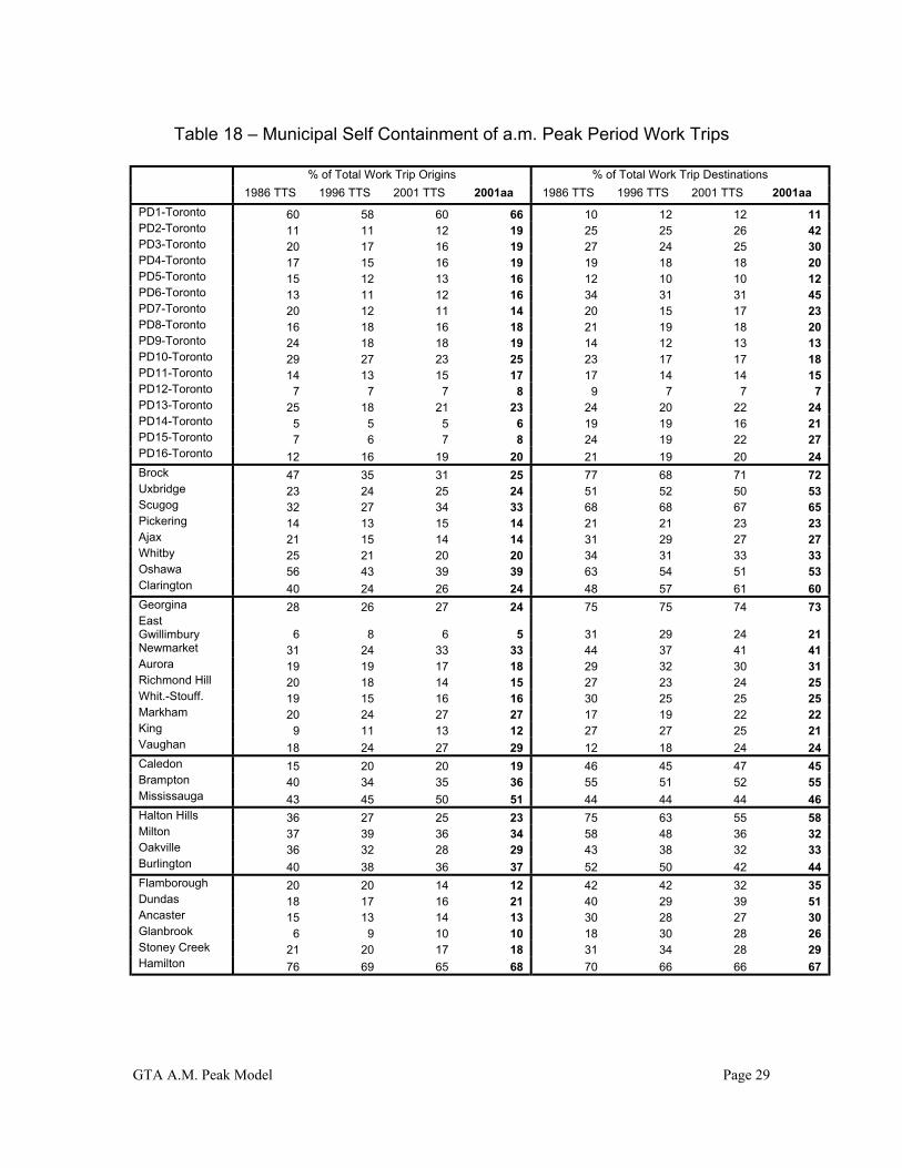
Municipal self containment (the number of trips that have both the origin and destination within the samemunicipal expressed as a percentage of the total origins or destinations for that municipality) is onemeasure that reflects the characteristics of the trip distribution and the amount of travel (person or vehicle

GTA A.M. Peak Model Page 28
km) that are being generated in total. A high self containment factor is desirable from the point of view ofminimising total travel demand.
Table 18 compares the base case simulated work trip self containment with the corresponding valuesobtained from the TTS data. The table is for the a.m. peak period and includes trips by all modes that have“work” as the destination trip purpose. Trips from work are excluded. Trips to and from areas outside theGTA and Hamilton are also excluded from the origin and destination totals throughout for consistency withthe TTS data. The observed values from the 1986, 1996 and 2001 surveys are included to give anindication of the historical trend.
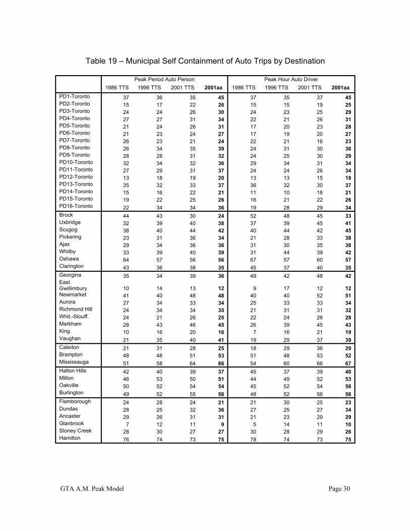
Table 19 is similar to Table 18 but for peak period auto person and peak hour auto driver trips by origin(generally the home end) only. The higher proportion of non-work trips should produce a slightly higherlevel of self containment in the simulation relative to the TTS data since non-work trips are, on average,less than half the length of work trips. The simulated peak hour driver trip matrix also includes the GO railauto egress, producing a further increase in peak hour self containment relative to the TTS.
GTA A.M. Peak Model Page 29
Table 18 – Municipal Self Containment of a.m. Peak Period Work Trips
% of Total Work Trip Origins % of Total Work Trip Destinations
1986 TTS 1996 TTS 2001 TTS 2001aa 1986 TTS 1996 TTS 2001 TTS 2001aa
PD1-Toronto 60 58 60 66 10 12 12 11PD2-Toronto 11 11 12 19 25 25 26 42PD3-Toronto 20 17 16 19 27 24 25 30PD4-Toronto 17 15 16 19 19 18 18 20PD5-Toronto 15 12 13 16 12 10 10 12PD6-Toronto 13 11 12 16 34 31 31 45PD7-Toronto 20 12 11 14 20 15 17 23PD8-Toronto 16 18 16 18 21 19 18 20PD9-Toronto 24 18 18 19 14 12 13 13PD10-Toronto 29 27 23 25 23 17 17 18PD11-Toronto 14 13 15 17 17 14 14 15PD12-Toronto 7 7 7 8 9 7 7 7PD13-Toronto 25 18 21 23 24 20 22 24PD14-Toronto 5 5 5 6 19 19 16 21PD15-Toronto 7 6 7 8 24 19 22 27PD16-Toronto 12 16 19 20 21 19 20 24Brock 47 35 31 25 77 68 71 72Uxbridge 23 24 25 24 51 52 50 53Scugog 32 27 34 33 68 68 67 65Pickering 14 13 15 14 21 21 23 23Ajax 21 15 14 14 31 29 27 27Whitby 25 21 20 20 34 31 33 33Oshawa 56 43 39 39 63 54 51 53Clarington 40 24 26 24 48 57 61 60Georgina 28 26 27 24 75 75 74 73EastGwillimbury 6 8 6 5 31 29 24 21Newmarket 31 24 33 33 44 37 41 41Aurora 19 19 17 18 29 32 30 31Richmond Hill 20 18 14 15 27 23 24 25Whit.-Stouff. 19 15 16 16 30 25 25 25Markham 20 24 27 27 17 19 22 22King 9 11 13 12 27 27 25 21Vaughan 18 24 27 29 12 18 24 24Caledon 15 20 20 19 46 45 47 45Brampton 40 34 35 36 55 51 52 55Mississauga 43 45 50 51 44 44 44 46Halton Hills 36 27 25 23 75 63 55 58Milton 37 39 36 34 58 48 36 32Oakville 36 32 28 29 43 38 32 33Burlington 40 38 36 37 52 50 42 44Flamborough 20 20 14 12 42 42 32 35Dundas 18 17 16 21 40 29 39 51Ancaster 15 13 14 13 30 28 27 30Glanbrook 6 9 10 10 18 30 28 26Stoney Creek 21 20 17 18 31 34 28 29Hamilton 76 69 65 68 70 66 66 67
GTA A.M. Peak Model Page 30
Table 19 – Municipal Self Containment of Auto Trips by Destination
Peak Period Auto Person Peak Hour Auto Driver
1986 TTS 1996 TTS 2001 TTS 2001aa 1986 TTS 1996 TTS 2001 TTS 2001aa
PD1-Toronto 37 36 35 45 37 35 37 45PD2-Toronto 15 17 22 26 15 15 19 25PD3-Toronto 24 24 26 30 24 23 25 29PD4-Toronto 27 27 31 34 22 21 26 31PD5-Toronto 21 24 26 31 17 20 23 28PD6-Toronto 21 23 24 27 17 19 20 27PD7-Toronto 26 23 21 24 22 21 16 23PD8-Toronto 26 34 35 39 24 31 30 36PD9-Toronto 28 28 31 32 24 25 30 29PD10-Toronto 32 34 32 36 29 34 31 34PD11-Toronto 27 29 31 37 24 24 26 34PD12-Toronto 13 18 19 20 13 13 15 18PD13-Toronto 35 32 33 37 36 32 30 37PD14-Toronto 15 16 22 21 11 10 18 21PD15-Toronto 19 22 25 26 16 21 22 26PD16-Toronto 22 34 34 36 19 28 29 34Brock 44 43 30 24 52 48 45 33Uxbridge 32 39 40 38 37 39 45 41Scugog 38 40 44 42 40 44 42 45Pickering 23 31 36 34 21 28 33 38Ajax 29 34 36 36 31 30 35 38Whitby 33 39 40 39 31 44 39 42Oshawa 64 57 56 56 67 57 60 57Clarington 43 36 38 35 45 37 40 35Georgina 35 34 39 36 49 42 48 42EastGwillimbury 10 14 13 12 9 17 12 12Newmarket 41 40 48 48 40 40 52 51Aurora 27 34 33 34 25 33 33 34Richmond Hill 24 34 34 35 21 31 31 32Whit.-Stouff. 24 21 26 25 22 24 26 28Markham 28 43 46 45 26 39 45 43King 10 16 20 16 7 16 21 19Vaughan 21 35 40 41 19 29 37 39Caledon 21 31 28 25 18 29 36 29Brampton 48 48 51 53 51 48 53 52Mississauga 51 58 64 66 54 60 66 67Halton Hills 42 40 39 37 45 37 39 40Milton 46 53 50 51 44 49 52 53Oakville 50 52 54 54 45 52 54 56Burlington 49 52 55 56 48 52 56 56Flamborough 24 28 24 21 21 30 25 23Dundas 28 25 32 36 27 25 27 34Ancaster 29 26 31 31 21 23 29 29Glanbrook 7 12 11 9 5 14 11 10Stoney Creek 28 30 27 27 30 28 29 26Hamilton 76 74 73 75 78 74 73 75
GTA A.M. Peak Model Page 31
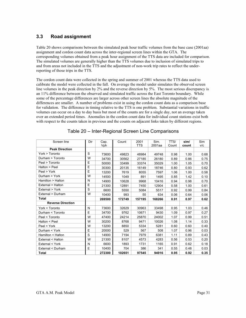
3.3 Road assignment
Table 20 shows comparisons between the simulated peak hour traffic volumes from the base case (2001aa)assignment and cordon count data across the inter-regional screen lines within the GTA. Thecorresponding volumes obtained from a peak hour assignment of the TTS data are included for comparison.The simulated volumes are generally higher than the TTS volumes due to inclusion of simulated trips toand from areas not included in the TTS and the adjustment of non-work trip rates to reflect the under-reporting of those trips in the TTS.
The cordon count data were collected in the spring and summer of 2001 whereas the TTS data used tocalibrate the model were collected in the fall. On average the model under simulates the observed screenline volumes in the peak direction by 2% and the reverse direction by 5%. The most serious discrepancy isan 11% difference between the observed and simulated traffic across the East Toronto boundary. Whilesome of the percentage differences are larger across other screen lines the absolute magnitude of thedifferences are smaller. A number of problems exist in using the cordon count data as a comparison basefor validation. The difference in timing relative to the TTS is one problem. Substantial variations in trafficvolumes can occur on a day to day basis but most of the counts are for a single day, not an average takenover an extended period times. Anomalies in the cordon count data for individual count stations exist bothwith respect to the counts taken in previous and the counts on adjacent links taken by different regions.
Table 20 – Inter-Regional Screen Line Comparisons
Screen line Dir Cap.Vph
Count 2001TTS
Sim.2001aa
TTS/Count
sim/count
Simv/c
Peak Direction
York > Toronto S 73600 49823 48984 49748 0.98 1.00 0.68Durham > Toronto W 34700 30562 27185 26180 0.89 0.86 0.75Peel > Toronto E 50000 33499 33374 35029 1.00 1.05 0.70Halton > Peel E 30300 20135 16149 18746 0.80 0.93 0.62Peel > York E 13200 7619 8055 7597 1.06 1.00 0.58Durham > York W 14500 1049 891 1495 0.85 1.42 0.10Hamilton > Halton N 14900 10628 9968 10416 0.94 0.98 0.70External > Halton E 21300 12891 7450 12904 0.58 1.00 0.61External > York S 6600 5550 5084 5517 0.92 0.99 0.84External > Durham W 10400 993 55 634 0.06 0.64 0.06Total 269500 172749 157195 168266 0.91 0.97 0.62
Reverse Direction
York < Toronto N 73600 32629 30963 33498 0.95 1.03 0.46
Durham < Toronto E 34700 9762 10671 9430 1.09 0.97 0.27
Peel < Toronto W 47400 24214 25870 24002 1.07 0.99 0.51
Halton < Peel W 30200 8768 9471 10026 1.08 1.14 0.33
Peel < York W 13200 8850 5334 5281 0.60 0.60 0.40
Durham < York E 20000 529 567 508 1.07 0.96 0.03
Hamilton < Halton S 14900 7194 7979 6381 1.11 0.89 0.43
External < Halton W 21300 8107 4573 4283 0.56 0.53 0.20
External < York N 6600 1893 1731 1165 0.91 0.62 0.18
External < Durham E 10400 704 386 341 0.55 0.48 0.03
Total 272300 102651 97545 94916 0.95 0.92 0.35
GTA A.M. Peak Model Page 32
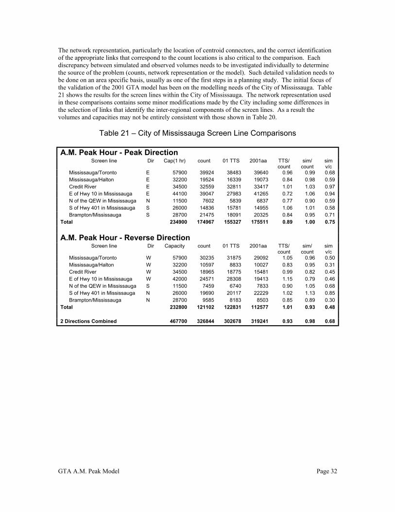
The network representation, particularly the location of centroid connectors, and the correct identificationof the appropriate links that correspond to the count locations is also critical to the comparison. Eachdiscrepancy between simulated and observed volumes needs to be investigated individually to determinethe source of the problem (counts, network representation or the model). Such detailed validation needs tobe done on an area specific basis, usually as one of the first steps in a planning study. The initial focus ofthe validation of the 2001 GTA model has been on the modelling needs of the City of Mississauga. Table21 shows the results for the screen lines within the City of Mississauga. The network representation usedin these comparisons contains some minor modifications made by the City including some differences inthe selection of links that identify the inter-regional components of the screen lines. As a result thevolumes and capacities may not be entirely consistent with those shown in Table 20.
Table 21 – City of Mississauga Screen Line Comparisons
A.M. Peak Hour - Peak DirectionScreen line Dir Cap(1 hr) count 01 TTS 2001aa TTS/
countsim/
countsimv/c
Mississauga/Toronto E 57900 39924 38483 39640 0.96 0.99 0.68Mississauga/Halton E 32200 19524 16339 19073 0.84 0.98 0.59Credit River E 34500 32559 32811 33417 1.01 1.03 0.97E of Hwy 10 in Mississauga E 44100 39047 27983 41265 0.72 1.06 0.94N of the QEW in Mississauga N 11500 7602 5839 6837 0.77 0.90 0.59S of Hwy 401 in Mississauga S 26000 14836 15781 14955 1.06 1.01 0.58Brampton/Mississauga S 28700 21475 18091 20325 0.84 0.95 0.71
Total 234900 174967 155327 175511 0.89 1.00 0.75
A.M. Peak Hour - Reverse DirectionScreen line Dir Capacity count 01 TTS 2001aa TTS/
countsim/
countsimv/c
Mississauga/Toronto W 57900 30235 31875 29092 1.05 0.96 0.50Mississauga/Halton W 32200 10597 8833 10027 0.83 0.95 0.31Credit River W 34500 18965 18775 15481 0.99 0.82 0.45E of Hwy 10 in Mississauga W 42000 24571 28308 19413 1.15 0.79 0.46N of the QEW in Mississauga S 11500 7459 6740 7833 0.90 1.05 0.68S of Hwy 401 in Mississauga N 26000 19690 20117 22229 1.02 1.13 0.85Brampton/Mississauga N 28700 9585 8183 8503 0.85 0.89 0.30
Total 232800 121102 122831 112577 1.01 0.93 0.48
2 Directions Combined 467700 326844 302678 319241 0.93 0.98 0.68
GTA A.M. Peak Model Page 33
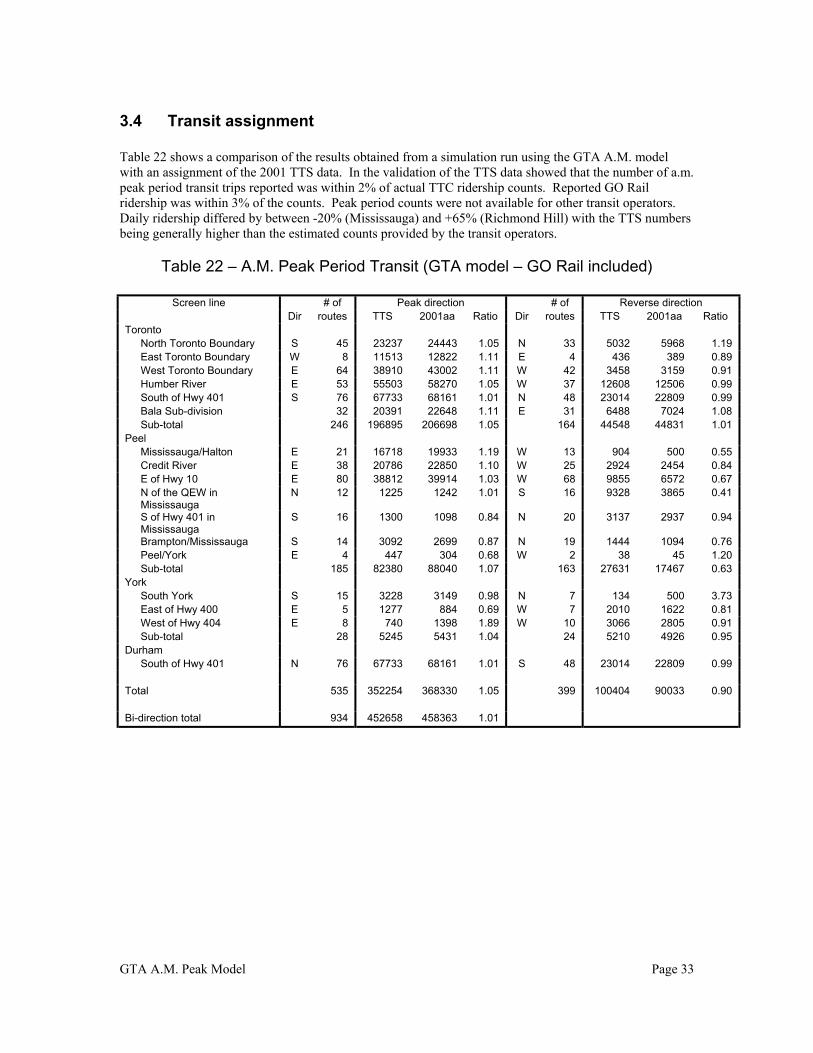
3.4 Transit assignment
Table 22 shows a comparison of the results obtained from a simulation run using the GTA A.M. modelwith an assignment of the 2001 TTS data. In the validation of the TTS data showed that the number of a.m.peak period transit trips reported was within 2% of actual TTC ridership counts. Reported GO Railridership was within 3% of the counts. Peak period counts were not available for other transit operators.Daily ridership differed by between -20% (Mississauga) and +65% (Richmond Hill) with the TTS numbersbeing generally higher than the estimated counts provided by the transit operators.
Table 22 – A.M. Peak Period Transit (GTA model – GO Rail included)
# of Peak direction # of Reverse directionScreen lineDir routes TTS 2001aa Ratio Dir routes TTS 2001aa Ratio
TorontoNorth Toronto Boundary S 45 23237 24443 1.05 N 33 5032 5968 1.19East Toronto Boundary W 8 11513 12822 1.11 E 4 436 389 0.89West Toronto Boundary E 64 38910 43002 1.11 W 42 3458 3159 0.91Humber River E 53 55503 58270 1.05 W 37 12608 12506 0.99South of Hwy 401 S 76 67733 68161 1.01 N 48 23014 22809 0.99Bala Sub-division 32 20391 22648 1.11 E 31 6488 7024 1.08Sub-total 246 196895 206698 1.05 164 44548 44831 1.01
PeelMississauga/Halton E 21 16718 19933 1.19 W 13 904 500 0.55Credit River E 38 20786 22850 1.10 W 25 2924 2454 0.84E of Hwy 10 E 80 38812 39914 1.03 W 68 9855 6572 0.67N of the QEW inMississauga
N 12 1225 1242 1.01 S 16 9328 3865 0.41
S of Hwy 401 inMississauga
S 16 1300 1098 0.84 N 20 3137 2937 0.94
Brampton/Mississauga S 14 3092 2699 0.87 N 19 1444 1094 0.76Peel/York E 4 447 304 0.68 W 2 38 45 1.20Sub-total 185 82380 88040 1.07 163 27631 17467 0.63
YorkSouth York S 15 3228 3149 0.98 N 7 134 500 3.73East of Hwy 400 E 5 1277 884 0.69 W 7 2010 1622 0.81West of Hwy 404 E 8 740 1398 1.89 W 10 3066 2805 0.91Sub-total 28 5245 5431 1.04 24 5210 4926 0.95
DurhamSouth of Hwy 401 N 76 67733 68161 1.01 S 48 23014 22809 0.99
Total 535 352254 368330 1.05 399 100404 90033 0.90
Bi-direction total 934 452658 458363 1.01
GTA A.M. Peak Model Page 34
4.0 Model Operation
4.1 Emme2bank
The emme2bank used to run the model may be a copy of an existing emme2bank already set up to run themodel or a new emme2bank can be created using the command “emme2 newbank”. If a new emme2bankis created it will need to be initialised with the required base matrices, zone ensemble and extra attributedata. The minimum recommended dimensions for a new emme2bank are shown in Table 23. Theemme2bank will use about 800 Mbytes of disk space.
Table 23 – Emme2bank DimensionsAttribute DimensionScenarios 20Centroids 1750Nodes 16,000Links 40,000Turns 8,000Transit vehicle types 10Transit lines 800Transit line segments 35,000Full matrices 50Origin matrices 200Destination matrices 200Scalars 999Functions per class 99Operators per function 2,000Log book 500Demarcation entries 100Extra attributes 1 million
If the same emme2bank is to be used to run the GTA p.m. model it is recommended that the minimumnumber of full matrices is increased to 150 and the minimum number of scenarios to 30. This largeremme2bank will require 1.3 Gbytes of disk space.
Matrices
The matrices used in the running of the model are identified by name, not number. The matrix numbersmay vary as each matrix is assigned to the first available number when first initiated. Matrix namesgenerally consist of 4 characters, the first 2 of which are always the letters “am”. The other two charactersare generally those used as the matrix number in the previous version of the model. An exception to theprevious naming convention is the scalars used to store the results of the transit assignment. These valuesresult from network calculations the output of which has to be stored in a scalar matrix identified by I.D.,not name. Appendix A contains a listing of the current matrix directory. Table 24 provides a summary ofthe current allocation by primary function.
The matrices used as input to the trip distribution component of the model have been pre-loaded along withthe base matrices containing the 2001 travel times and GO Rail egress trips. For most applications of themodel these matrices do not require modification and should be protected from accidental modification.The matrices are listed in Table 25. It is important to remember than cell values in the base matrices usedas input to the trip distribution represent relative probabilities, not trips. They include values for cellswhere the existing row and/or column trip totals are zero. The matrices must be balanced to the requiredrow and column trip totals before a meaningful trip assignment can be performed.
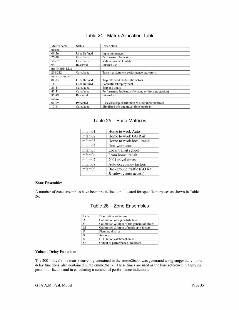
GTA A.M. Peak Model Page 35
Table 24 - Matrix Allocation Table
Matrix name Status Descriptionmsam01-26 User Defined Input parameters27-58 Calculated Performance Indicators59-67 Calculated Validation check totals99 Reserved Internal usems (Matrix I.D.)201-212 Calculated Transit assignment performance indicatorsmoam or mdam01-13 User Defined Trip rates and mode split factors18 User Defined Population/Employment20-41 Calculated Trip end totals42-51 Calculated Performance Indicators (by zone or link aggregation)97-99 Reserved Internal usemfam01-09 Protected Base case trip distribution & other input matrices17-31 Calculated Simulated trip and travel time matrices
Table 25 – Base Matrices
mfam01 Home to work Automfam02 Home to work GO Railmfam03 Home to work local transitmfam04 Non-work automfam05 Local transit schoolmfam06 From home transitmfam07 2001 travel timesmfam08 Auto occupancy factorsmfam09 Background traffic (GO Rail
& subway auto access)
Zone Ensembles
A number of zone ensembles have been pre-defined or allocated for specific purposes as shown in Table26.
Table 26 – Zone Ensembles
Letter Description and/or useA Calibration of trip distributionG Calibration & Input of trip generation RatesM Calibration & Input of mode split factorsP Planning districtR RegionsS GO Station catchment areasQ Output of performance indicators
Volume Delay Functions
The 2001-travel time matrix currently contained in the emme2bank was generated using tangential volumedelay functions, also contained in the emme2bank. These times are used as the base reference in applyingpeak hour factors and in calculating a number of performance indicators.
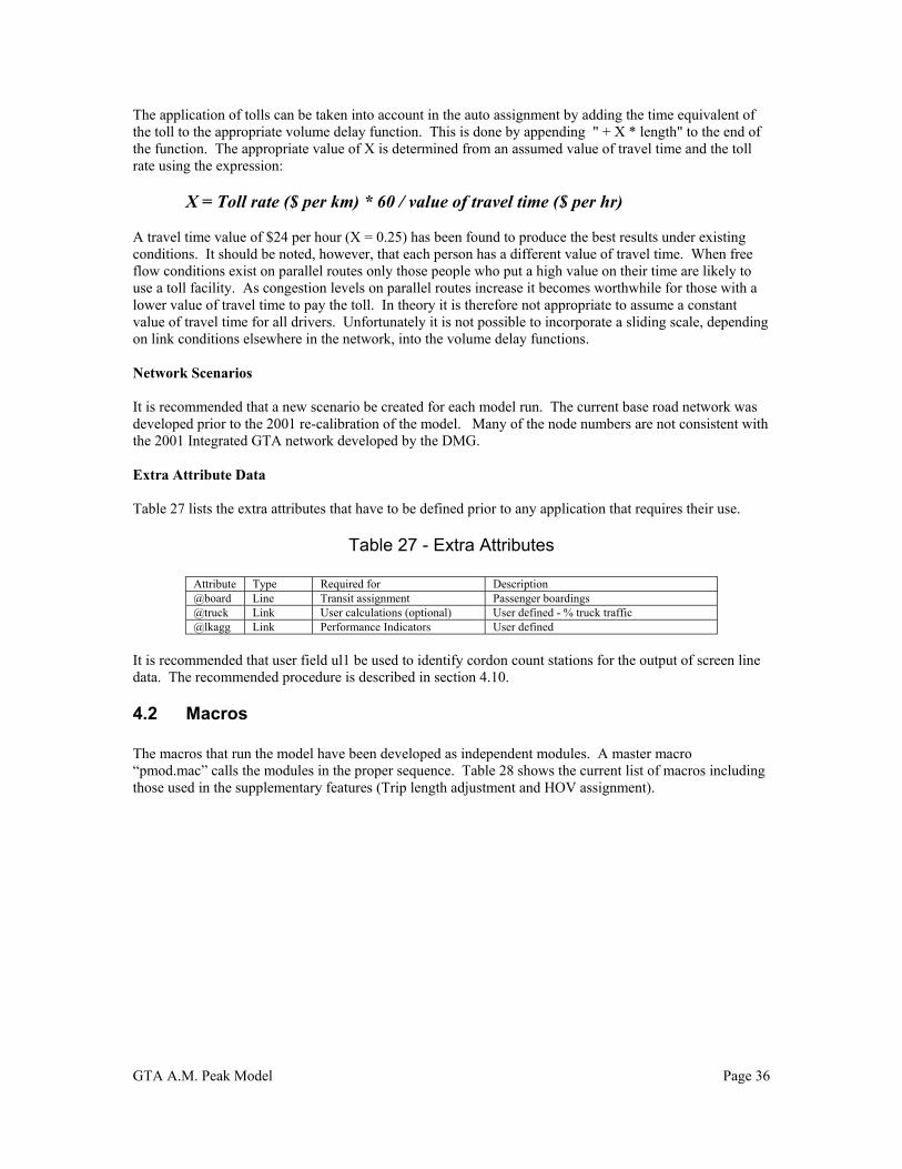
GTA A.M. Peak Model Page 36
The application of tolls can be taken into account in the auto assignment by adding the time equivalent ofthe toll to the appropriate volume delay function. This is done by appending " + X * length" to the end ofthe function. The appropriate value of X is determined from an assumed value of travel time and the tollrate using the expression:
X = Toll rate ($ per km) * 60 / value of travel time ($ per hr)
A travel time value of $24 per hour (X = 0.25) has been found to produce the best results under existingconditions. It should be noted, however, that each person has a different value of travel time. When freeflow conditions exist on parallel routes only those people who put a high value on their time are likely touse a toll facility. As congestion levels on parallel routes increase it becomes worthwhile for those with alower value of travel time to pay the toll. In theory it is therefore not appropriate to assume a constantvalue of travel time for all drivers. Unfortunately it is not possible to incorporate a sliding scale, dependingon link conditions elsewhere in the network, into the volume delay functions.
Network Scenarios
It is recommended that a new scenario be created for each model run. The current base road network wasdeveloped prior to the 2001 re-calibration of the model. Many of the node numbers are not consistent withthe 2001 Integrated GTA network developed by the DMG.
Extra Attribute Data
Table 27 lists the extra attributes that have to be defined prior to any application that requires their use.
Table 27 - Extra Attributes
Attribute Type Required for Description@board Line Transit assignment Passenger boardings@truck Link User calculations (optional) User defined - % truck traffic@lkagg Link Performance Indicators User defined
It is recommended that user field ul1 be used to identify cordon count stations for the output of screen linedata. The recommended procedure is described in section 4.10.
4.2 Macros
The macros that run the model have been developed as independent modules. A master macro“pmod.mac” calls the modules in the proper sequence. Table 28 shows the current list of macros includingthose used in the supplementary features (Trip length adjustment and HOV assignment).
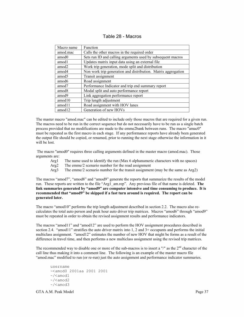
GTA A.M. Peak Model Page 37
Table 28 - Macros
Macro name Functionamod.mac Calls the other macros in the required orderamod0 Sets run ID and calling arguments used by subsequent macrosamod1 Updates matrix input data using an external fileamod2 Work trip generation, mode split and distributionamod4 Non work trip generation and distribution. Matrix aggregationamod5 Transit assignmentamod6 Road assignmentamod7 Performance Indicator and trip end summary reportamod8 Modal split and auto performance reportamod9 Link aggregation performance reportamod10 Trip length adjustmentamod11 Road assignment with HOV lanesamod12 Generation of new HOVs
The master macro "amod.mac" can be edited to include only those macros that are required for a given run.The macros need to be run in the correct sequence but do not necessarily have to be run as a single batchprocess provided that no modifications are made to the emme2bank between runs. The macro "amac0"must be repeated as the first macro in each stage. If any performance reports have already been generatedthe output file should be copied, or renamed, prior to running the next stage otherwise the information in itwill be lost.
The macro "amod0" requires three calling arguments defined in the master macro (amod.mac). Thosearguments are:
Arg1 The name used to identify the run (Max 6 alphanumeric characters with no spaces)Arg2 The emme/2 scenario number for the road assignmentArg3 The emme/2 scenario number for the transit assignment (may be the same as Arg2)
The macros “amod7”, “amod8” and “amod9” generate the reports that summarize the results of the modelrun. These reports are written to the file “Arg1_am.rep”. Any previous file of that name is deleted. Thelink summaries generated by “amod9” are computer intensive and time consuming to produce. It isrecommended that “amod9” be skipped if a fast turn around is required. The report can begenerated later.
The macro “amod10” performs the trip length adjustment described in section 2.2. The macro also re-calculates the total auto person and peak hour auto driver trip matrices. Macros “amod6” through “amod9”must be repeated in order to obtain the revised assignment results and performance indicators.
The macros “amod11” and “amod12” are used to perform the HOV assignment procedures described insection 2.4. “amod11” stratifies the auto driver matrix into 1, 2 and 3+ occupants and performs the initialmulticlass assignment. “amod12” estimates the number of new HOV that might be forms as a result of thedifference in travel time, and then performs a new multiclass assignment using the revised trip matrices.
The recommended way to disable one or more of the sub-macros is to insert a "/" as the 2nd character of thecall line thus making it into a comment line. The following is an example of the master macro file“amod.mac” modified to run (or re-run) just the auto assignment and performance indicator summaries.
username~<amod0 2001aa 2001 2001~/<amod1~/<amod2~/<amod3

GTA A.M. Peak Model Page 38
~/<amod4~/<amod5~<amod6~<amod7~<amod8~<amod9q
The following command line will execute the above macro in batch mode.emme2 -m amod.mac batch >&filename&
Where "filename" is a temporary file used for output of the emme2 dialog.
4.3 Input Data
The macro "amod1" reads matrix input data contained in the file "x_am", where "x" is the first argumentused to call "amod0". This file may be used to selectively modify the simulation parameters (msam01through msam26), enter population and employment data and to redefine the trip generation rates and/ormode split factors as desired. It is recommended that matrices requiring change be deleted and re-createdrather than modifying the values in the existing matrix. The macro will then run even if the there is noexisting matrix of that name whereas attempting to modify a non-existing matrix will cause a fatal area. Ifmodifying an existing matrix it is important to remember that only the cells that are specified are changed.It is therefore essential to include zero values in the list.
The basic inputs required for a model run are a network and land use data (population and employment) byzone. The population data must be stored as origin matrix moam18 and the employment data as destinationmatrix mdam18. The population and employment data is usually imported in the "x_am" file at the start ofthe model run.
Table 29 provides a list of the other input parameters that can be modified, together with recommendedvalues for the years 2001, 2006, 2011, 2016 and 2021. The 2021 values are also recommended forsubsequent years. The recommended method of modification is to include specification of the desiredscalar matrices and values in the "x_am" file for each model run. Any scalars not included will retain thevalues from the previous run.
It is recommended that a new "x_am" file be created for each model run using an appropriate name toidentify the year and development scenario. The file should be saved, along with the output summaryreport, in order to provide a complete record of the input data for that model run. Every "x_am" file shouldinclude specification of values for all of the scalars listed in Table 29 as well as any origin or destinationvectors that may be selectively modified for different years or simulation scenarios. The inclusion of allthe scalar values in the appropriate "x_am" file will help prevent the accidental use of the wrong valuesfrom a previous run.
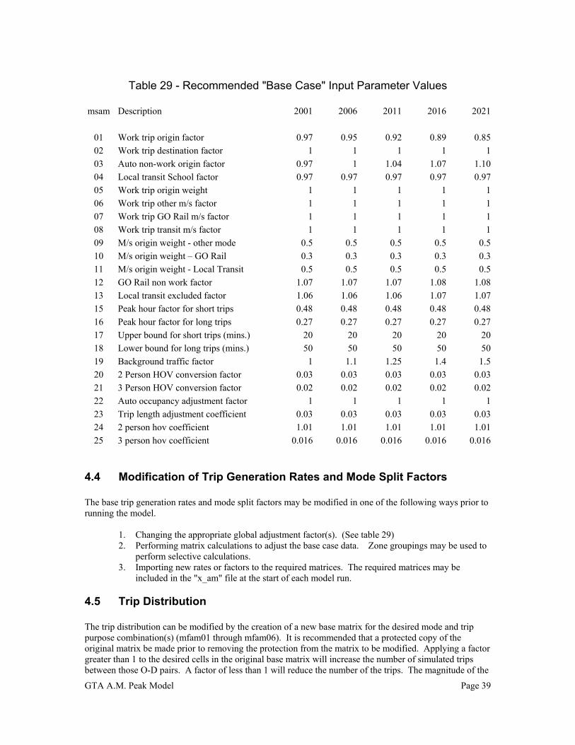
GTA A.M. Peak Model Page 39
Table 29 - Recommended "Base Case" Input Parameter Values
msam Description 2001 2006 2011 2016 2021
01 Work trip origin factor 0.97 0.95 0.92 0.89 0.85
02 Work trip destination factor 1 1 1 1 1
03 Auto non-work origin factor 0.97 1 1.04 1.07 1.10
04 Local transit School factor 0.97 0.97 0.97 0.97 0.97
05 Work trip origin weight 1 1 1 1 1
06 Work trip other m/s factor 1 1 1 1 1
07 Work trip GO Rail m/s factor 1 1 1 1 1
08 Work trip transit m/s factor 1 1 1 1 1
09 M/s origin weight - other mode 0.5 0.5 0.5 0.5 0.5
10 M/s origin weight – GO Rail 0.3 0.3 0.3 0.3 0.3
11 M/s origin weight - Local Transit 0.5 0.5 0.5 0.5 0.5
12 GO Rail non work factor 1.07 1.07 1.07 1.08 1.08
13 Local transit excluded factor 1.06 1.06 1.06 1.07 1.07
15 Peak hour factor for short trips 0.48 0.48 0.48 0.48 0.48
16 Peak hour factor for long trips 0.27 0.27 0.27 0.27 0.27
17 Upper bound for short trips (mins.) 20 20 20 20 20
18 Lower bound for long trips (mins.) 50 50 50 50 50
19 Background traffic factor 1 1.1 1.25 1.4 1.5
20 2 Person HOV conversion factor 0.03 0.03 0.03 0.03 0.03
21 3 Person HOV conversion factor 0.02 0.02 0.02 0.02 0.02
22 Auto occupancy adjustment factor 1 1 1 1 1
23 Trip length adjustment coefficient 0.03 0.03 0.03 0.03 0.03
24 2 person hov coefficient 1.01 1.01 1.01 1.01 1.01
25 3 person hov coefficient 0.016 0.016 0.016 0.016 0.016
4.4 Modification of Trip Generation Rates and Mode Split Factors
The base trip generation rates and mode split factors may be modified in one of the following ways prior torunning the model.
1. Changing the appropriate global adjustment factor(s). (See table 29)2. Performing matrix calculations to adjust the base case data. Zone groupings may be used to
perform selective calculations.3. Importing new rates or factors to the required matrices. The required matrices may be
included in the "x_am" file at the start of each model run.
4.5 Trip Distribution
The trip distribution can be modified by the creation of a new base matrix for the desired mode and trippurpose combination(s) (mfam01 through mfam06). It is recommended that a protected copy of theoriginal matrix be made prior to removing the protection from the matrix to be modified. Applying a factorgreater than 1 to the desired cells in the original base matrix will increase the number of simulated tripsbetween those O-D pairs. A factor of less than 1 will reduce the number of the trips. The magnitude of the
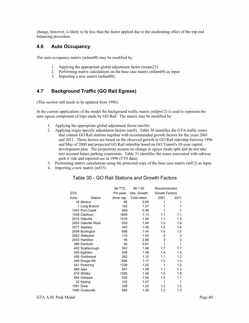
GTA A.M. Peak Model Page 40
change, however, is likely to be less than the factor applied due to the moderating effect of the trip endbalancing procedure.
4.6 Auto Occupancy
The auto occupancy matrix (mfam08) may be modified by:
1. Applying the appropriate global adjustment factor (msam22).2. Performing matrix calculations on the base case matrix (mfam08) as input3. Importing a new matrix (mfam08).
4.7 Background Traffic (GO Rail Egress)
(This section still needs to be updated from 1996).
In the current applications of the model the background traffic matrix (mfpm12) is used to represent theauto egress component of trips made by GO Rail. The matrix may be modified by:
1. Applying the appropriate global adjustment factor (ms36).2. Applying origin specific adjustment factors (mo9). Table 30 identifies the GTA traffic zones
that contain GO Rail stations together with recommended growth factors for the years 2001and 2011. These factors are based on the observed growth in GO Rail ridership between 1996and May of 2000 and projected GO Rail ridership based on GO Transit's 10-year capitaldevelopment plan. The projections assume no change in egress mode split and do not takeinto account future parking constraints. Table 31 identifies the zones associated with subwaypark n' ride and reported use in 1996 (TTS data).
3. Performing matrix calculations using the protected copy of the base case matrix (mf12) as input.4. Importing a new matrix (mf15)
Table 30 - GO Rail Stations and Growth Factors
96 TTS 96 > 00 Recommended
GTA Pm peak Obs. Growth Growth Factors
Zone Station driver egr. Total riders 2001 201116 Mimico 66 0.95 1 1
1 Long Branch 102 1.07 1 11547 Port Credit 849 0.96 1 11539 Clarkson 1809 1.13 1.1 1.12014 Oakville 1416 1.06 1.1 1.52003 Oakville West 509 1.44 1.5 1.62077 Appleby 443 1.48 1.5 1.62059 Burlington 698 1.44 1.5 1.52052 Aldershot 110 1.63 2 22520 Hamilton 95 2.88 3 3
368 Danforth 60 0.81 1 1402 Scarborough 502 1.66 1.7 1.7405 Eglinton 438 1.38 1.4 1.5458 Guildwood 262 1.12 1.1 1.2449 Rouge Hill 694 1.17 1.2 1.3541 Pickering 1338 1.02 1 1.5569 Ajax 851 1.08 1.1 1.3616 Whitby 1085 1.48 1.5 1.8664 Oshawa 526 1.54 1.5 1.7
22 Kipling 102 1.07 1 11561 Dixie 338 1.25 1.3 1.31566 Cooksville 684 1.28 1.3 1.3
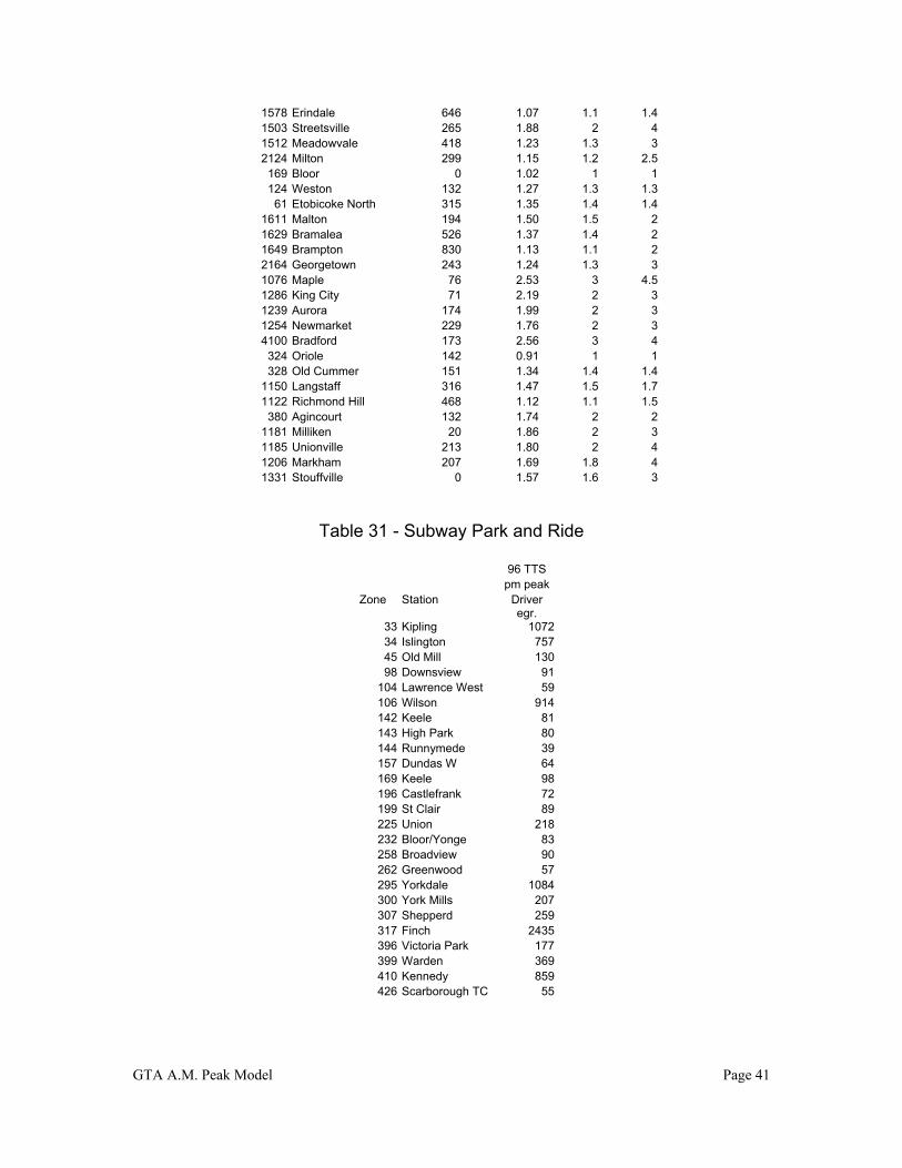
GTA A.M. Peak Model Page 41
1578 Erindale 646 1.07 1.1 1.41503 Streetsville 265 1.88 2 41512 Meadowvale 418 1.23 1.3 32124 Milton 299 1.15 1.2 2.5
169 Bloor 0 1.02 1 1124 Weston 132 1.27 1.3 1.3
61 Etobicoke North 315 1.35 1.4 1.41611 Malton 194 1.50 1.5 21629 Bramalea 526 1.37 1.4 21649 Brampton 830 1.13 1.1 22164 Georgetown 243 1.24 1.3 31076 Maple 76 2.53 3 4.51286 King City 71 2.19 2 31239 Aurora 174 1.99 2 31254 Newmarket 229 1.76 2 34100 Bradford 173 2.56 3 4
324 Oriole 142 0.91 1 1328 Old Cummer 151 1.34 1.4 1.4
1150 Langstaff 316 1.47 1.5 1.71122 Richmond Hill 468 1.12 1.1 1.5
380 Agincourt 132 1.74 2 21181 Milliken 20 1.86 2 31185 Unionville 213 1.80 2 41206 Markham 207 1.69 1.8 41331 Stouffville 0 1.57 1.6 3
Table 31 - Subway Park and Ride
96 TTSpm peak
Zone Station Driveregr.
33 Kipling 107234 Islington 75745 Old Mill 13098 Downsview 91
104 Lawrence West 59106 Wilson 914142 Keele 81143 High Park 80144 Runnymede 39157 Dundas W 64169 Keele 98196 Castlefrank 72199 St Clair 89225 Union 218232 Bloor/Yonge 83258 Broadview 90262 Greenwood 57295 Yorkdale 1084300 York Mills 207307 Shepperd 259317 Finch 2435396 Victoria Park 177399 Warden 369410 Kennedy 859426 Scarborough TC 55

GTA A.M. Peak Model Page 42
4.8 Other Adjustment Factors
Other factors that can be adjusted prior to a model run are:
1. The weight assigned to the work trip origin total relative to the work trip destination total.2. The weight assigned to the origin trip totals by mode relative to the destination total for the
same mode.3. GO Rail non-work factor.4. Local transit excluded factor.
Refer to Table 29 or Appendix A in order to identify the appropriate matrix scalars.
4.9 Model Outputs
The primary outputs from a simulation run are the trip matrices and network assignments. Analysis of theresults is possible within emme/2 or selected data may be exported for external analysis. Assignmentresults will remain in the emme2bank until the applicable scenario is deleted, modified or used for anothermodel run. Subsequent model runs will over write matrix information.
The macro “amod7” produces a report listing the values of all the matrix scalars contained in theemme2bank. This report can be used as a permanent record of the input parameters, control totals,calculated trip totals and global performance indicators.
The macros “amod7” and “amod8” produce reports that summarise trip data by the zone groups containedin zone ensemble “gq”. Figure 4 shows the groupings as they are currently defined in the emme2bank.
Figure 6 - Aggregations Used for Output Summaries(To be added)
The macro “amod7” produces two reports containing the following information
Report 1• Population. Employment Total trip origins Work tip destinations Non-work destinations
Report 2 GO Rail origins Local transit origins Auto person origins Peak hour auto driver origins GO Rail destinations Local transit destinations Auto person destinations Peak hour auto driver destinations
Calculated performance indicators contained in the report produced by “amod8”• Activity rate (jobs per 1000 population) Origin transit modal split (all trips) Destination transit mode split (all trips) Self-containment (% of all trip destinations that have their origin within the same zone group).

GTA A.M. Peak Model Page 43
Mean auto person trip time by destination based on 1996 Levels of Service. Mean auto person trip time by destination based on the projected level of service given by an
equilibrium assignment to a future network. Mean auto occupancy by destination
The macro “amod9” calculates totals and averages for link aggregations defined by non-zero values of theextra link attribute "@lkagg". The report that is produced contains the following for each category of link.
Number of links in the aggregation Total assigned vehicle km Total assigned vehicle hours Mean speed (kph) Capacity utilisation (assigned vehicle km / vehicle km of capacity) Total link volume Volume to capacity ratio
The calculation of capacity utilisation differs from volume to capacity ratio in that the length of each link inthe aggregation is used to weight the result. Capacity utilisation is the appropriate measure to use as theaverage for a geographic area.
The link categories may be used to define screen lines, geographic areas, categories of road, or anycombinations of these attributes. The extra link attribute “@lkagg” must be created prior to running“amod9”.
The output reports are generated using the standard emme/2 output modules 3.12 and 3.14. There are somelimitations inherent in that format.
The emme/2 report format shows the sum, mean, minimum and maximum values at the end ofeach table. The mean value shown is an un-weighted average that does not take into accountthe different sizes of the aggregations.
Origin and destination vectors are used to store the results of the calculations for each linkaggregation. The zone numbers shown are the reference numbers for each link aggregationsused in these vectors. There is no relationship to actual zones or zone system other than that azone numbers must be defined as centroids in the network in order for them to be used asvalid reference numbers.
Other matrix and link attribute data may be exported for external analysis using modules 3.14 and 2.41...
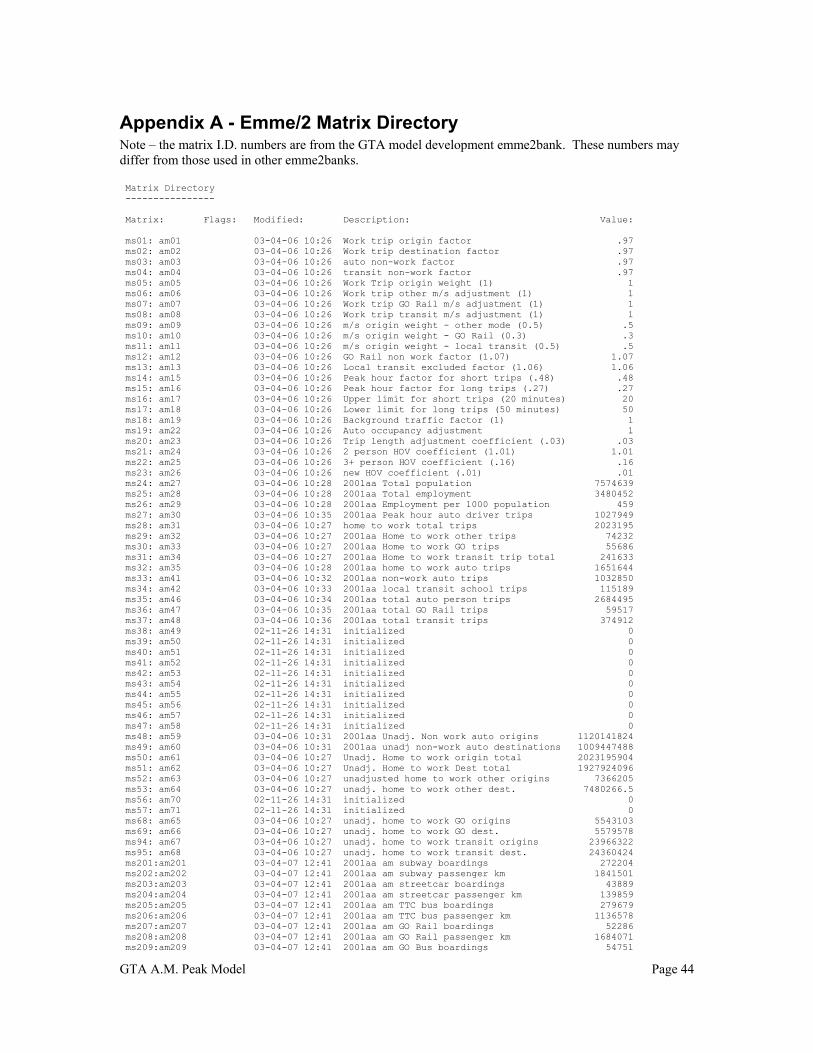
GTA A.M. Peak Model Page 44
Appendix A - Emme/2 Matrix DirectoryNote – the matrix I.D. numbers are from the GTA model development emme2bank. These numbers maydiffer from those used in other emme2banks.
Matrix Directory ----------------
Matrix: Flags: Modified: Description: Value:
ms01: am01 03-04-06 10:26 Work trip origin factor .97 ms02: am02 03-04-06 10:26 Work trip destination factor .97 ms03: am03 03-04-06 10:26 auto non-work factor .97 ms04: am04 03-04-06 10:26 transit non-work factor .97 ms05: am05 03-04-06 10:26 Work Trip origin weight (1) 1 ms06: am06 03-04-06 10:26 Work trip other m/s adjustment (1) 1 ms07: am07 03-04-06 10:26 Work trip GO Rail m/s adjustment (1) 1 ms08: am08 03-04-06 10:26 Work trip transit m/s adjustment (1) 1 ms09: am09 03-04-06 10:26 m/s origin weight - other mode (0.5) .5 ms10: am10 03-04-06 10:26 m/s origin weight - GO Rail (0.3) .3 ms11: am11 03-04-06 10:26 m/s origin weight - local transit (0.5) .5 ms12: am12 03-04-06 10:26 GO Rail non work factor (1.07) 1.07 ms13: am13 03-04-06 10:26 Local transit excluded factor (1.06) 1.06 ms14: am15 03-04-06 10:26 Peak hour factor for short trips (.48) .48 ms15: am16 03-04-06 10:26 Peak hour factor for long trips (.27) .27 ms16: am17 03-04-06 10:26 Upper limit for short trips (20 minutes) 20 ms17: am18 03-04-06 10:26 Lower limit for long trips (50 minutes) 50 ms18: am19 03-04-06 10:26 Background traffic factor (1) 1 ms19: am22 03-04-06 10:26 Auto occupancy adjustment 1 ms20: am23 03-04-06 10:26 Trip length adjustment coefficient (.03) .03 ms21: am24 03-04-06 10:26 2 person HOV coefficient (1.01) 1.01 ms22: am25 03-04-06 10:26 3+ person HOV coefficient (.16) .16 ms23: am26 03-04-06 10:26 new HOV coefficient (.01) .01 ms24: am27 03-04-06 10:28 2001aa Total population 7574639 ms25: am28 03-04-06 10:28 2001aa Total employment 3480452 ms26: am29 03-04-06 10:28 2001aa Employment per 1000 population 459 ms27: am30 03-04-06 10:35 2001aa Peak hour auto driver trips 1027949 ms28: am31 03-04-06 10:27 home to work total trips 2023195 ms29: am32 03-04-06 10:27 2001aa Home to work other trips 74232 ms30: am33 03-04-06 10:27 2001aa Home to work GO trips 55686 ms31: am34 03-04-06 10:27 2001aa Home to work transit trip total 241633 ms32: am35 03-04-06 10:28 2001aa home to work auto trips 1651644 ms33: am41 03-04-06 10:32 2001aa non-work auto trips 1032850 ms34: am42 03-04-06 10:33 2001aa local transit school trips 115189 ms35: am46 03-04-06 10:34 2001aa total auto person trips 2684495 ms36: am47 03-04-06 10:35 2001aa total GO Rail trips 59517 ms37: am48 03-04-06 10:36 2001aa total transit trips 374912 ms38: am49 02-11-26 14:31 initialized 0 ms39: am50 02-11-26 14:31 initialized 0 ms40: am51 02-11-26 14:31 initialized 0 ms41: am52 02-11-26 14:31 initialized 0 ms42: am53 02-11-26 14:31 initialized 0 ms43: am54 02-11-26 14:31 initialized 0 ms44: am55 02-11-26 14:31 initialized 0 ms45: am56 02-11-26 14:31 initialized 0 ms46: am57 02-11-26 14:31 initialized 0 ms47: am58 02-11-26 14:31 initialized 0 ms48: am59 03-04-06 10:31 2001aa Unadj. Non work auto origins 1120141824 ms49: am60 03-04-06 10:31 2001aa unadj non-work auto destinations 1009447488 ms50: am61 03-04-06 10:27 Unadj. Home to work origin total 2023195904 ms51: am62 03-04-06 10:27 Unadj. Home to work Dest total 1927924096 ms52: am63 03-04-06 10:27 unadjusted home to work other origins 7366205 ms53: am64 03-04-06 10:27 unadj. home to work other dest. 7480266.5 ms56: am70 02-11-26 14:31 initialized 0 ms57: am71 02-11-26 14:31 initialized 0 ms68: am65 03-04-06 10:27 unadj. home to work GO origins 5543103 ms69: am66 03-04-06 10:27 unadj. home to work GO dest. 5579578 ms94: am67 03-04-06 10:27 unadj. home to work transit origins 23966322 ms95: am68 03-04-06 10:27 unadj. home to work transit dest. 24360424 ms201:am201 03-04-07 12:41 2001aa am subway boardings 272204 ms202:am202 03-04-07 12:41 2001aa am subway passenger km 1841501 ms203:am203 03-04-07 12:41 2001aa am streetcar boardings 43889 ms204:am204 03-04-07 12:41 2001aa am streetcar passenger km 139859 ms205:am205 03-04-07 12:41 2001aa am TTC bus boardings 279679 ms206:am206 03-04-07 12:41 2001aa am TTC bus passenger km 1136578 ms207:am207 03-04-07 12:41 2001aa am GO Rail boardings 52286 ms208:am208 03-04-07 12:41 2001aa am GO Rail passenger km 1684071 ms209:am209 03-04-07 12:41 2001aa am GO Bus boardings 54751
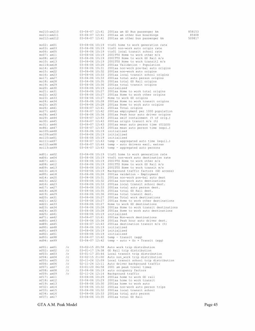
GTA A.M. Peak Model Page 45
ms210:am210 03-04-07 12:41 2001aa am GO Bus passenger km 858153 ms211:am211 03-04-07 12:41 2001aa am other bus boardings 85408 ms212:am212 03-04-07 12:41 2001aa am other bus passenger km 509817
mo02: am01 03-04-06 10:19 tts01 home to work generation rate mo03: am03 03-04-06 10:19 tts01 non-work auto origin rate mo06: am05 03-04-06 10:19 tts01 local transit school rate mo07: am11 03-04-06 10:19 2001TTS Home to work other m/s mo08: am12 03-04-06 10:19 2001TTS Home to work GO Rail m/s mo10: am13 03-04-06 10:19 2001TTS Home to work transitl m/s mo114:am18 03-04-06 10:26 2001aa Validation - Population mo14: am20 03-04-06 10:31 2001aa non-work pre-bal auto origins mo15: am22 03-04-06 10:32 2001aa non-work auto origins mo16: am23 03-04-06 10:33 2001aa local transit school origins mo17: am27 03-04-06 10:33 2001aa total auto person origins mo18: am28 03-04-06 10:35 2001aa total GO Rail origins mo19: am29 03-04-06 10:36 2001aa total transit origins mo20: am30 03-04-06 10:19 initialized mo21: am31 03-04-06 10:27 2001aa Home to work total origins mo22: am32 03-04-06 10:27 2001aa Home to work other origins mo23: am33 03-04-06 10:27 Home to work GO origins mo24: am34 03-04-06 10:28 2001aa Home to work transit origins mo25: am35 03-04-06 10:28 2001aa Home to work auto origins mo26: am41 03-04-07 12:41 2001aa Total origins mo27: am42 03-04-07 12:42 2001aa employment per 1000 population mo28: am43 03-04-06 10:34 2001aa Peak hour auto driver origins mo29: am44 03-04-07 12:43 2001aa self containment (% of orig.) mo30: am45 03-04-07 12:43 2001aa origin transit m/s (%) mo31: am46 03-04-07 12:43 2001aa mean auto person time (01LOS) mo86: am47 03-04-07 12:43 2001aa mean auto person time (equi.) mo105:am48 03-04-06 10:19 initialized mo109:am50 03-04-06 10:19 initialized mo110:am51 03-04-06 10:19 initialized mo111:am97 03-04-07 12:43 temp - aggregated auto time (equil.) mo112:am98 03-04-07 12:44 temp - auto drivers excl. extras mo113:am99 03-04-07 12:43 temp - aggregated auto persons
md01: am02 03-04-06 10:19 tts01 home to work generation rate md06: am04 03-04-06 10:19 tts01 non-work auto destination rate md07: am11 03-04-06 10:19 2001TTS Home to work other m/s md08: am12 03-04-06 10:19 2001TTS Home to work GO Rail m/s md09: am13 03-04-06 10:19 2001TTS Home to work transit m/s md10: am14 03-04-06 10:19 Background traffic factors (GO access) md95: am18 03-04-06 10:26 2001aa vaidation - Employment md14: am20 03-04-06 10:31 2001aa non-work pre-bal auto dest md15: am22 03-04-06 10:32 2001aa non-work auto destinations md16: am23 03-04-06 10:33 2001aa local transit school dest. md17: am27 03-04-06 10:33 2001aa total auto person dest. md18: am28 03-04-06 10:35 2001aa total GO Rail dest. md19: am29 03-04-06 10:36 2001aa total transit dest. md20: am31 03-04-06 10:27 2001aa Total work destinations md21: am32 03-04-06 10:27 2001aa Home to work other destinations md22: am33 03-04-06 10:27 Home to work GO destinations md23: am34 03-04-06 10:28 2001aa Home to work transit destinations md24: am35 03-04-06 10:28 2001aa Home to work auto destinations md25: am41 03-04-06 10:19 initialized md71: am42 03-04-07 12:41 2001aa Non-work destinations md80: am43 03-04-06 10:34 2001aa Peak hour auto driver dest. md89: am45 03-04-07 12:43 2001aa destination transit m/s (%) md90: am48 03-04-06 10:19 initialized md91: am49 03-04-06 10:19 initialized md92: am51 03-04-06 10:19 initialized md93: am98 03-04-07 12:42 temp - transit (agg) md94: am99 03-04-07 12:42 temp - auto + Go + Transit (agg)
mf01: am01 /r 03-02-15 20:58 Auto work trip distribution mf02: am02 /r 03-01-17 19:38 GO Rail trip distribution mf03: am03 /r 03-01-17 20:44 Local transit trip distribution mf04: am04 /r 03-02-15 21:00 Auto non_work trip distribution mf05: am05 /r 02-11-24 12:09 Local transit school trip distribution mf06: am06 /r 02-11-24 12:11 Auto driver background traffic mf07: am07 /r 03-01-20 06:58 2001 am peak travel times mf08: am08 /r 03-04-06 10:19 auto occupancy factors mf09: am09 /r 02-11-24 12:14 Background traffic mf17: am11 03-04-06 10:29 2001aa home to work GO rail mf18: am12 03-04-06 10:29 2001aa home to work transit mf19: am13 03-04-06 10:30 2001aa home to work auto mf32: am14 03-04-06 10:32 2001aa non-work auto person trips mf33: am15 03-04-06 10:32 2001aa local transit school mf34: am16 03-04-06 10:33 2001aa total auto person mf37: am17 03-04-06 10:35 2001aa total GO Rail

GTA A.M. Peak Model Page 46
mf99: am18 03-04-06 10:35 2001aa total transit mf100:am21 03-04-06 10:56 2001aa auto travel times mf103:am27 03-04-06 10:34 2001aa Peak hour auto driver trips mf104:am31 03-04-06 10:31 temp non-work auto origins
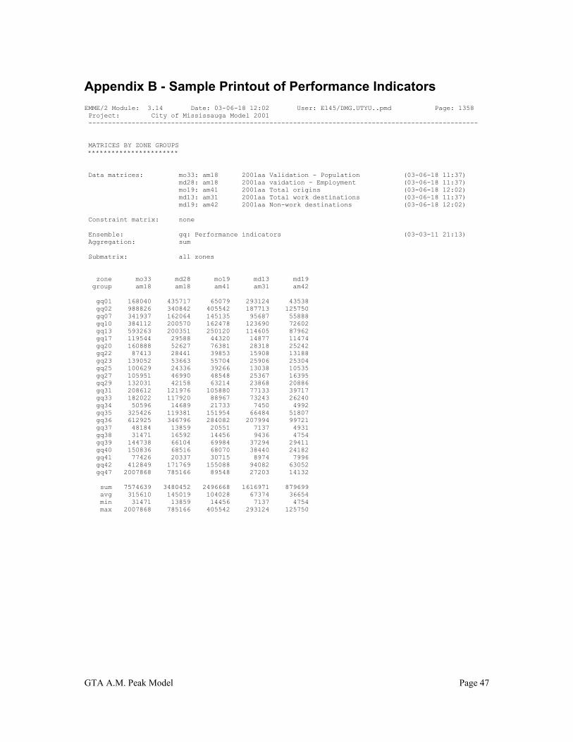
GTA A.M. Peak Model Page 47
Appendix B - Sample Printout of Performance Indicators
EMME/2 Module: 3.14 Date: 03-06-18 12:02 User: E145/DMG.UTYU..pmd Page: 1358 Project: City of Mississauga Model 2001 ---------------------------------------------------------------------------------------------------
MATRICES BY ZONE GROUPS ***********************
Data matrices: mo33: am18 2001aa Validation - Population (03-06-18 11:37) md28: am18 2001aa vaidation - Employment (03-06-18 11:37) mo19: am41 2001aa Total origins (03-06-18 12:02) md13: am31 2001aa Total work destinations (03-06-18 11:37) md19: am42 2001aa Non-work destinations (03-06-18 12:02)
Constraint matrix: none
Ensemble: gq: Performance indicators (03-03-11 21:13) Aggregation: sum
Submatrix: all zones
zone mo33 md28 mo19 md13 md19 group am18 am18 am41 am31 am42
gq01 168040 435717 65079 293124 43538 gq02 988826 340842 405542 187713 125750 gq07 341937 162064 145135 95687 55888 gq10 384112 200570 162478 123690 72602 gq13 593263 200351 250120 114605 87962 gq17 119544 29588 44320 14877 11474 gq20 160888 52627 76381 28318 25242 gq22 87413 28441 39853 15908 13188 gq23 139052 53663 55704 25906 25304 gq25 100629 24336 39266 13038 10535 gq27 105951 46990 48548 25367 16395 gq29 132031 42158 63214 23868 20886 gq31 208612 121976 105880 77133 39717 gq33 182022 117920 88967 73243 26240 gq34 50596 14689 21733 7450 4992 gq35 325426 119381 151954 66484 51807 gq36 612925 346796 284082 207994 99721 gq37 48184 13859 20551 7137 4931 gq38 31471 16592 14456 9436 4754 gq39 144738 66104 69984 37294 29411 gq40 150836 68516 68070 38440 24182 gq41 77426 20337 30715 8974 7996 gq42 412849 171769 155088 94082 63052 gq47 2007868 785166 89548 27203 14132
sum 7574639 3480452 2496668 1616971 879699 avg 315610 145019 104028 67374 36654 min 31471 13859 14456 7137 4754 max 2007868 785166 405542 293124 125750
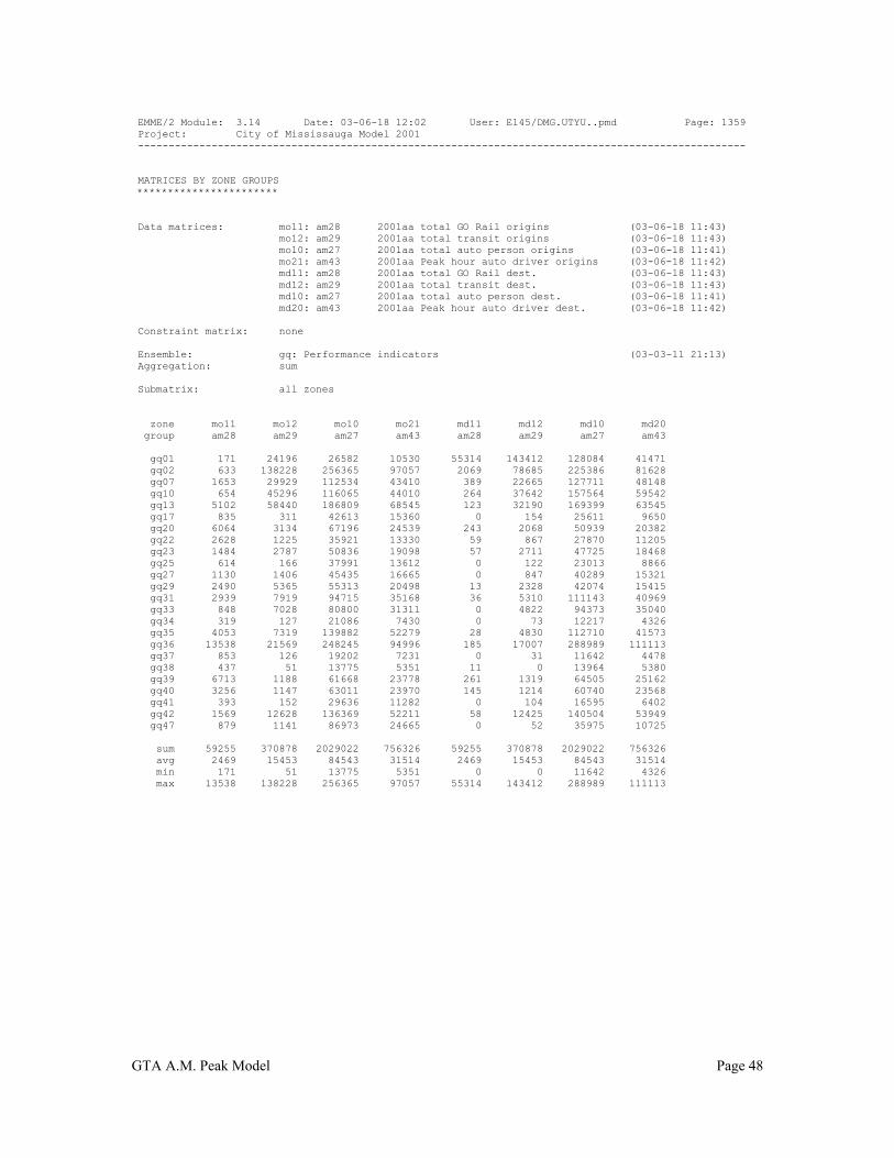
GTA A.M. Peak Model Page 48
EMME/2 Module: 3.14 Date: 03-06-18 12:02 User: E145/DMG.UTYU..pmd Page: 1359 Project: City of Mississauga Model 2001 ---------------------------------------------------------------------------------------------------
MATRICES BY ZONE GROUPS ***********************
Data matrices: mo11: am28 2001aa total GO Rail origins (03-06-18 11:43) mo12: am29 2001aa total transit origins (03-06-18 11:43) mo10: am27 2001aa total auto person origins (03-06-18 11:41) mo21: am43 2001aa Peak hour auto driver origins (03-06-18 11:42) md11: am28 2001aa total GO Rail dest. (03-06-18 11:43) md12: am29 2001aa total transit dest. (03-06-18 11:43) md10: am27 2001aa total auto person dest. (03-06-18 11:41) md20: am43 2001aa Peak hour auto driver dest. (03-06-18 11:42)
Constraint matrix: none
Ensemble: gq: Performance indicators (03-03-11 21:13) Aggregation: sum
Submatrix: all zones
zone mo11 mo12 mo10 mo21 md11 md12 md10 md20 group am28 am29 am27 am43 am28 am29 am27 am43
gq01 171 24196 26582 10530 55314 143412 128084 41471 gq02 633 138228 256365 97057 2069 78685 225386 81628 gq07 1653 29929 112534 43410 389 22665 127711 48148 gq10 654 45296 116065 44010 264 37642 157564 59542 gq13 5102 58440 186809 68545 123 32190 169399 63545 gq17 835 311 42613 15360 0 154 25611 9650 gq20 6064 3134 67196 24539 243 2068 50939 20382 gq22 2628 1225 35921 13330 59 867 27870 11205 gq23 1484 2787 50836 19098 57 2711 47725 18468 gq25 614 166 37991 13612 0 122 23013 8866 gq27 1130 1406 45435 16665 0 847 40289 15321 gq29 2490 5365 55313 20498 13 2328 42074 15415 gq31 2939 7919 94715 35168 36 5310 111143 40969 gq33 848 7028 80800 31311 0 4822 94373 35040 gq34 319 127 21086 7430 0 73 12217 4326 gq35 4053 7319 139882 52279 28 4830 112710 41573 gq36 13538 21569 248245 94996 185 17007 288989 111113 gq37 853 126 19202 7231 0 31 11642 4478 gq38 437 51 13775 5351 11 0 13964 5380 gq39 6713 1188 61668 23778 261 1319 64505 25162 gq40 3256 1147 63011 23970 145 1214 60740 23568 gq41 393 152 29636 11282 0 104 16595 6402 gq42 1569 12628 136369 52211 58 12425 140504 53949 gq47 879 1141 86973 24665 0 52 35975 10725
sum 59255 370878 2029022 756326 59255 370878 2029022 756326 avg 2469 15453 84543 31514 2469 15453 84543 31514 min 171 51 13775 5351 0 0 11642 4326 max 13538 138228 256365 97057 55314 143412 288989 111113
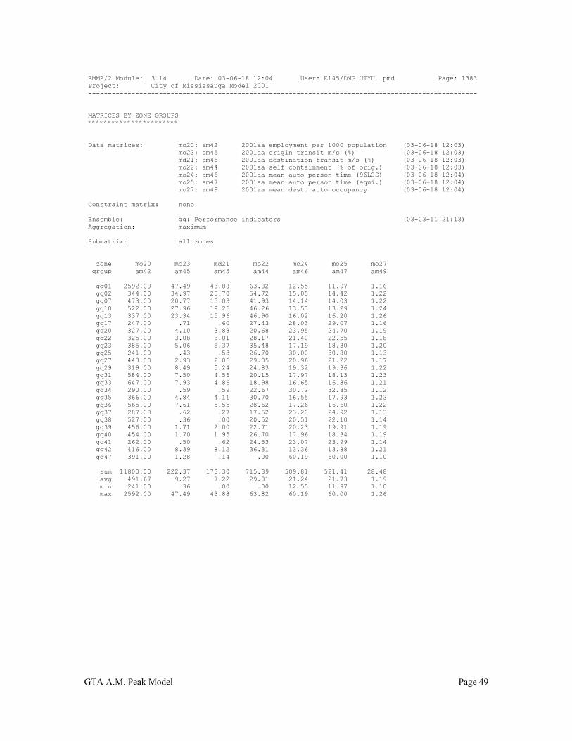
GTA A.M. Peak Model Page 49
EMME/2 Module: 3.14 Date: 03-06-18 12:04 User: E145/DMG.UTYU..pmd Page: 1383 Project: City of Mississauga Model 2001 ---------------------------------------------------------------------------------------------------
MATRICES BY ZONE GROUPS ***********************
Data matrices: mo20: am42 2001aa employment per 1000 population (03-06-18 12:03) mo23: am45 2001aa origin transit m/s (%) (03-06-18 12:03) md21: am45 2001aa destination transit m/s (%) (03-06-18 12:03) mo22: am44 2001aa self containment (% of orig.) (03-06-18 12:03) mo24: am46 2001aa mean auto person time (96LOS) (03-06-18 12:04) mo25: am47 2001aa mean auto person time (equi.) (03-06-18 12:04) mo27: am49 2001aa mean dest. auto occupancy (03-06-18 12:04)
Constraint matrix: none
Ensemble: gq: Performance indicators (03-03-11 21:13) Aggregation: maximum
Submatrix: all zones
zone mo20 mo23 md21 mo22 mo24 mo25 mo27 group am42 am45 am45 am44 am46 am47 am49
gq01 2592.00 47.49 43.88 63.82 12.55 11.97 1.16 gq02 344.00 34.97 25.70 54.72 15.05 14.42 1.22 gq07 473.00 20.77 15.03 41.93 14.14 14.03 1.22 gq10 522.00 27.96 19.26 46.26 13.53 13.29 1.24 gq13 337.00 23.34 15.96 46.90 16.02 16.20 1.26 gq17 247.00 .71 .60 27.43 28.03 29.07 1.16 gq20 327.00 4.10 3.88 20.68 23.95 24.70 1.19 gq22 325.00 3.08 3.01 28.17 21.40 22.55 1.18 gq23 385.00 5.06 5.37 35.48 17.19 18.30 1.20 gq25 241.00 .43 .53 26.70 30.00 30.80 1.13 gq27 443.00 2.93 2.06 29.05 20.96 21.22 1.17 gq29 319.00 8.49 5.24 24.83 19.32 19.36 1.22 gq31 584.00 7.50 4.56 20.15 17.97 18.13 1.23 gq33 647.00 7.93 4.86 18.98 16.65 16.86 1.21 gq34 290.00 .59 .59 22.67 30.72 32.85 1.12 gq35 366.00 4.84 4.11 30.70 16.55 17.93 1.23 gq36 565.00 7.61 5.55 28.62 17.26 16.60 1.22 gq37 287.00 .62 .27 17.52 23.20 24.92 1.13 gq38 527.00 .36 .00 20.52 20.51 22.10 1.14 gq39 456.00 1.71 2.00 22.71 20.23 19.91 1.19 gq40 454.00 1.70 1.95 26.70 17.96 18.34 1.19 gq41 262.00 .50 .62 24.53 23.07 23.99 1.14 gq42 416.00 8.39 8.12 36.31 13.36 13.88 1.21 gq47 391.00 1.28 .14 .00 60.19 60.00 1.10
sum 11800.00 222.37 173.30 715.39 509.81 521.41 28.48 avg 491.67 9.27 7.22 29.81 21.24 21.73 1.19 min 241.00 .36 .00 .00 12.55 11.97 1.10 max 2592.00 47.49 43.88 63.82 60.19 60.00 1.26

GTA A.M. Peak Model Page 50
Appendix C – Trip Distribution Validation Plots
Comparisons between simulated and 2001 TTS data
• Auto work trip travel time distributions
• Auto work trip link scattergram -
• Auto non-work trip travel time distribution
• Auto non-work trip link scattergram
• GO Train work trip travel time distribution
• Local transit work trip travel time distribution
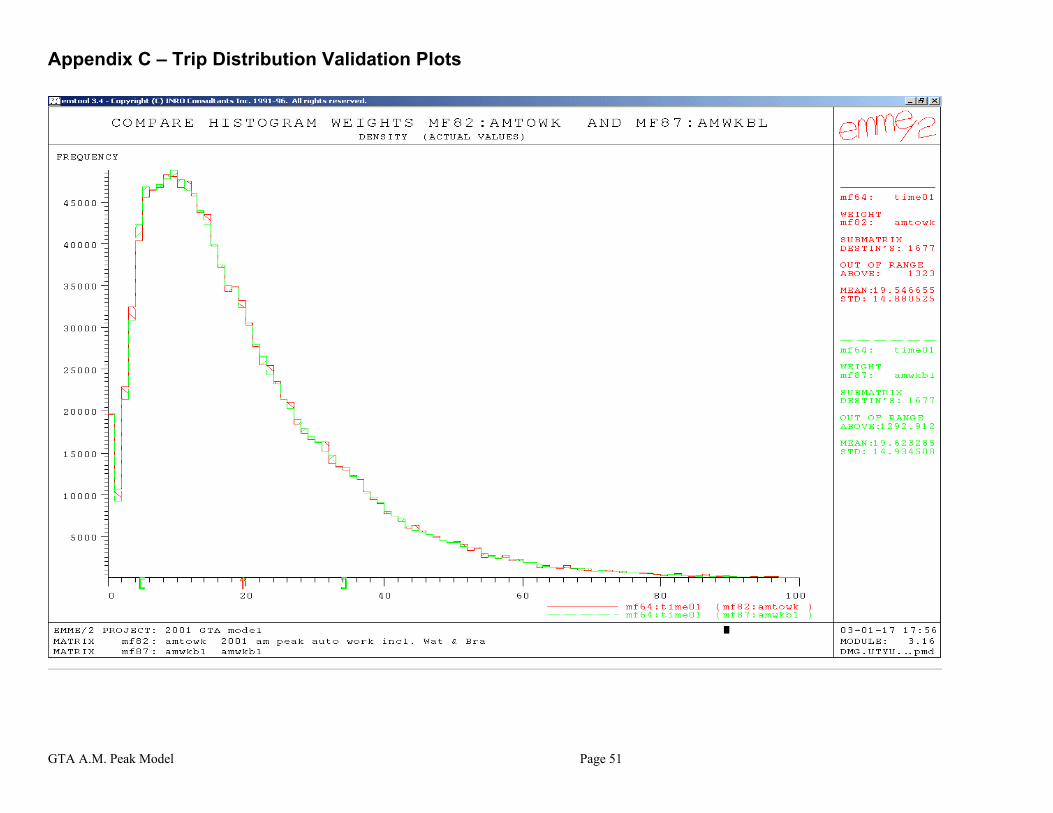
Appendix C – Trip Distribution Validation Plots
GTA A.M. Peak Model Page 51
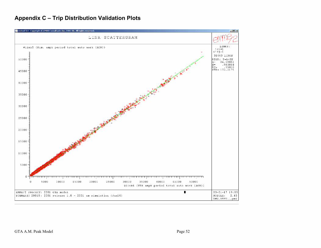
Appendix C – Trip Distribution Validation Plots
GTA A.M. Peak Model Page 52
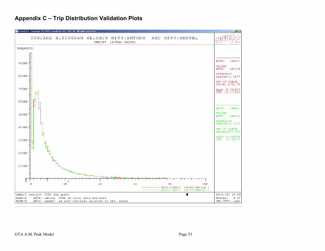
Appendix C – Trip Distribution Validation Plots
GTA A.M. Peak Model Page 53
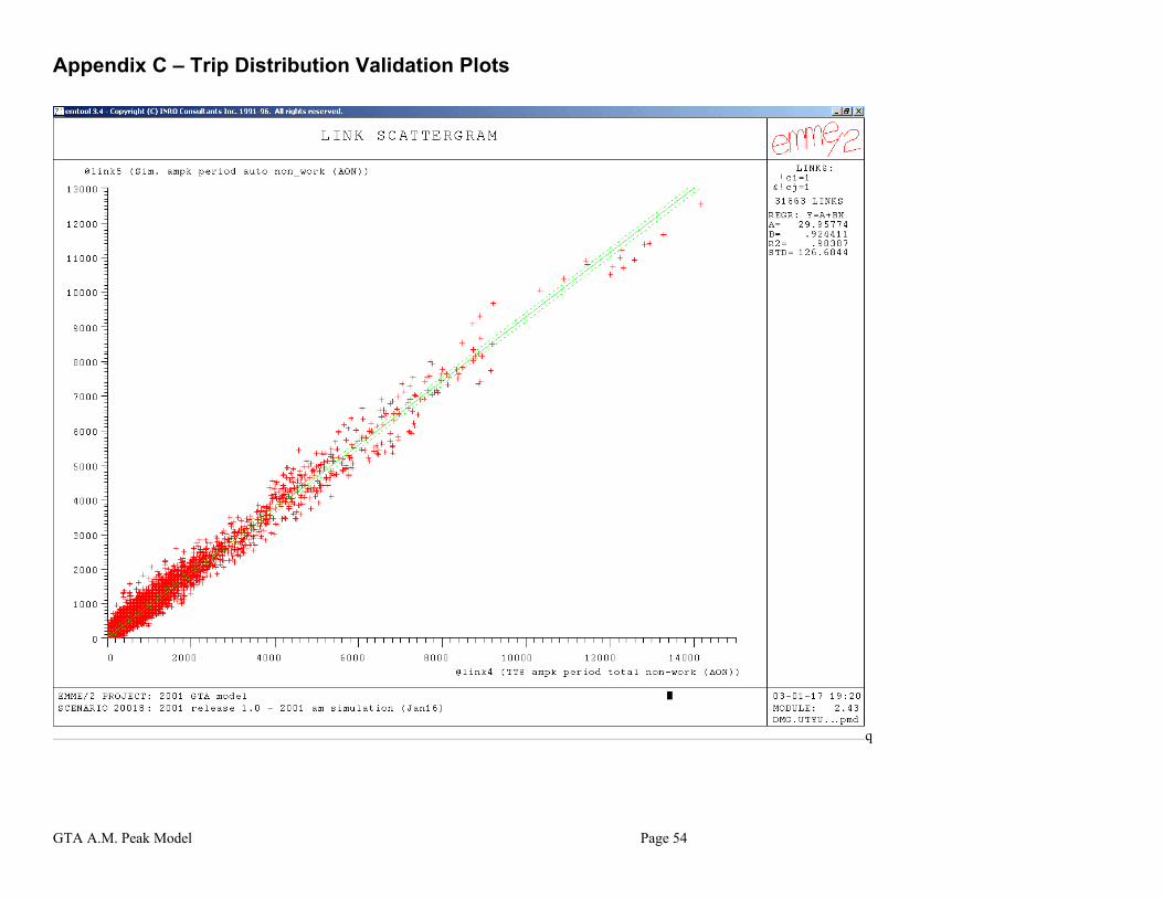
Appendix C – Trip Distribution Validation Plots
GTA A.M. Peak Model Page 54
q
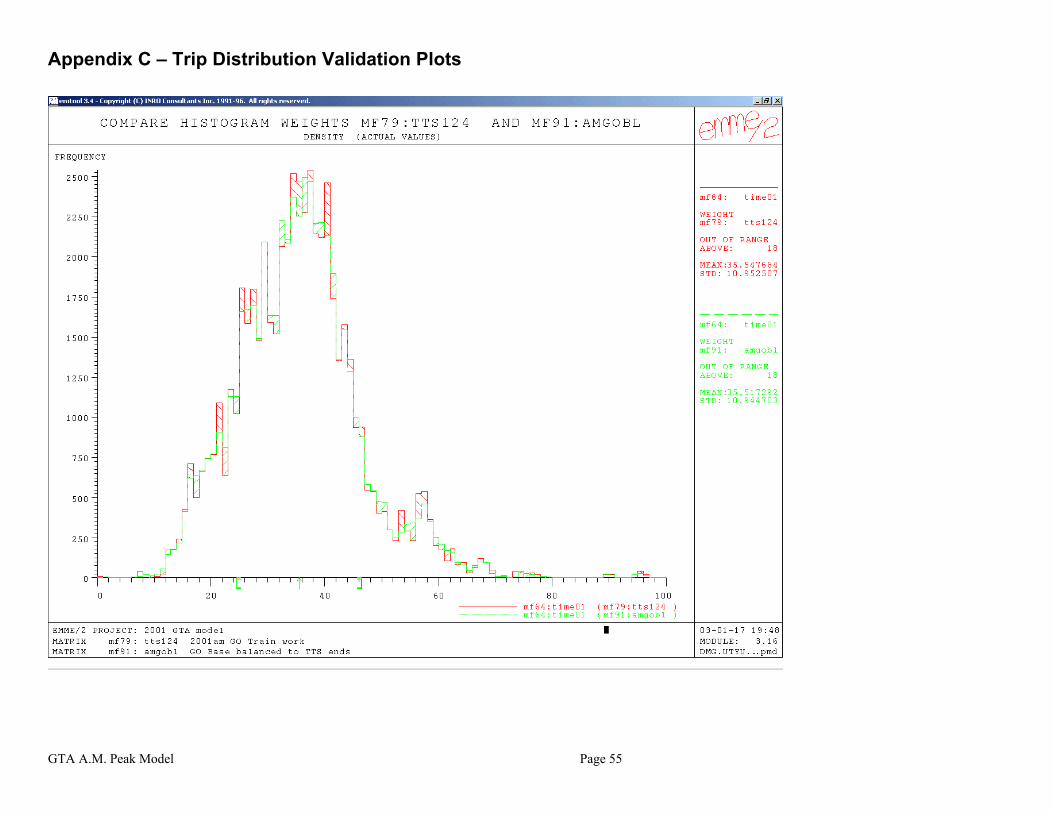
Appendix C – Trip Distribution Validation Plots
GTA A.M. Peak Model Page 55
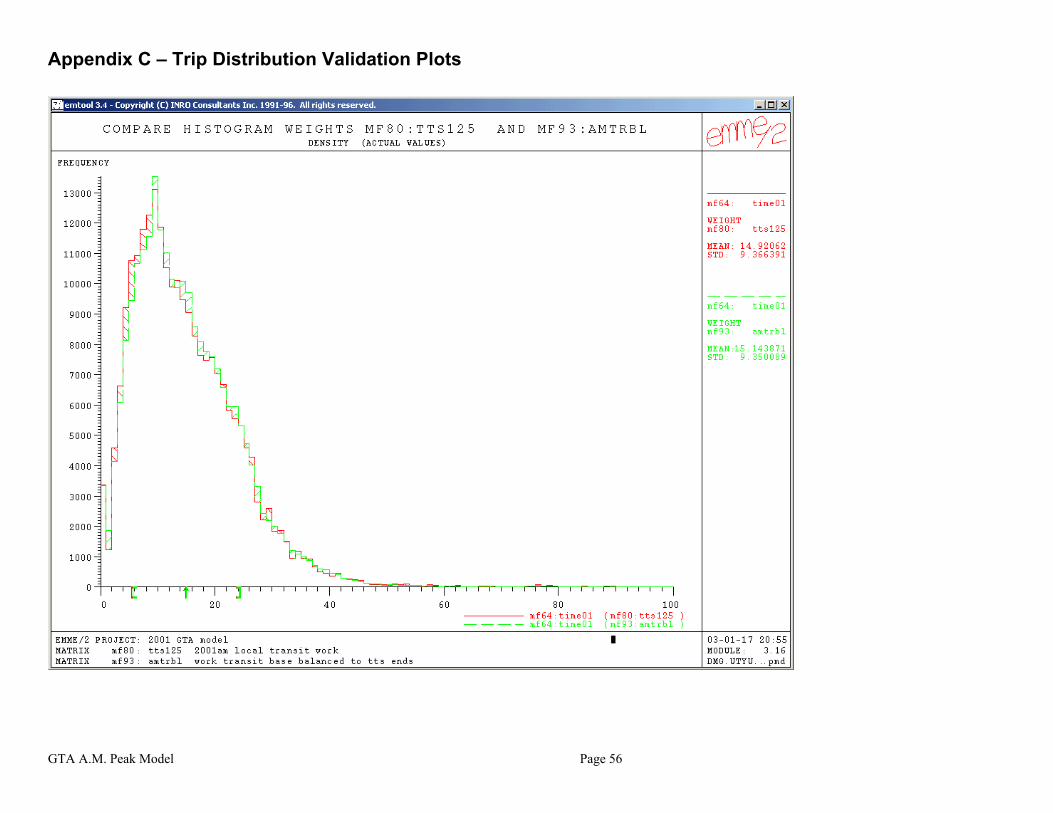
Appendix C – Trip Distribution Validation Plots
GTA A.M. Peak Model Page 56