Embed Size (px)
Citation preview

ĠSTANBUL TECHNICAL UNIVERSITY INSTITUTE OF SCIENCE AND TECHNOLOGY
M.Sc. Thesis by
Duygu Merve ÖZALTIN
Department : Electronics and Telecommunication Engineering
Programme : Telecommunication Engineering
JUNE 2009
RECONSTRUCTION OF COMPLEX PERMITTIVITY OF AN
INHOMOGENEOUS MATERIAL IN A RECTANGULAR WAVEGUIDE


ĠSTANBUL TECHNICAL UNIVERSITY INSTITUTE OF SCIENCE AND TECHNOLOGY
M.Sc. Thesis by
Duygu Merve ÖZALTIN
(504071305)
Date of submission : 04 May 2009
Date of defence examination: 04 June 2009
Supervisor (Chairman) : Assoc. Prof. Dr. Ali YAPAR (ITU)
Members of the Examining Committee : Prof. Dr. Ġbrahim AKDUMAN (ITU)
Assis. Prof. Dr. Lale Tükenmez
ERGENE (ITU)
JUNE 2009
RECONSTRUCTION OF COMPLEX PERMITTIVITY OF AN
INHOMOGENEOUS MATERIAL IN A RECTANGULAR WAVEGUIDE


Haziran 2009
ĠSTANBUL TEKNĠK ÜNĠVERSĠTESĠ FEN BĠLĠMLERĠ ENSTĠTÜSÜ
YÜKSEK LĠSANS TEZĠ
Duygu Merve ÖZALTIN
(504071305)
Tezin Enstitüye Verildiği Tarih : 04 Mayıs 2009
Tezin Savunulduğu Tarih : 04 Haziran 2009
Tez Danışmanı : Doç. Dr. Ali YAPAR (ĠTÜ)
Diğer Jüri Üyeleri : Prof. Dr. Ġbrahim AKDUMAN (ĠTÜ)
Yrd. Doç. Dr. Lale Tükenmez ERGENE
(ĠTÜ)
DĠKDÖRTGEN DALGAKILAVUZU ĠÇERĠSĠNDEKĠ HOMOJEN
OLMAYAN BĠR MADDENĠN KOMPLEKS GEÇĠRGENLĠK DEĞERĠNĠN
BELĠRLENMESĠ

v
FOREWORD
I would like to express my appreciation and thanks for my advisor Assoc. Prof. Dr. Ali
Yapar who gave me the opportunity to work under his supervision.
I would like to express my gratitude to Assoc. Prof. Dr. Funda Akleman Yapar who never
hesitated to help me when I needed her guidance. I would also like to thank to Prof. Dr.
İbrahim Akduman and all members of Electromagnetic Research Group.
I would like to thank to my family for their endless support.
Finally, I would like thank to TUBITAK (The Scientific and Technological Research
Council of Turkey) for supporting me financially by the project 108E146.
June 2009
Duygu Merve ÖZALTIN
Telecommunication Engineer

vi

vii
TABLE OF CONTENTS
Page
ABBREVIATIONS ................................................................................................. viii
LIST OF FIGURES .................................................................................................. ix
SUMMARY ............................................................................................................... xi
ÖZET ........................................................................................................................ xiii
1. INTRODUCTION .................................................................................................. 1
1.1 Purpose of the Thesis ......................................................................................... 3
2. FORWARD SCATTERING PROBLEM ............................................................ 5
2.1 Problem Description ........................................................................................... 5
2.2 Dyadic Green’s Function for Rectangular Waveguide ...................................... 6
2.3 Method of Moments ........................................................................................... 8
2.4 Finite Difference Time Domain ....................................................................... 11
2.4.1 One-Dimensional FDTD ........................................................................... 11
2.4.2 Three-Dimensional FDTD - Yee’s Algorithm .......................................... 13
2.5 Mode Matching ................................................................................................ 17
2.6 Numerical Results ............................................................................................ 18
3. INVERSE SCATTERING PROBLEM ............................................................. 23
3.1 Statement of the Problem ................................................................................. 23
3.2 Contrast Source Inversion Method ................................................................... 24
3.3 Numerical Results ............................................................................................ 28
4. CONCLUSION AND RECOMMENDATIONS ............................................... 35
REFERENCES ......................................................................................................... 37

viii
ABBREVIATIONS
CG : Conjugate Gradient
CSI : Contrast Source Inversion
MoM : Method of Moments
FDTD : Finite Difference Time Domain

ix
LIST OF FIGURES
Page
Figure 2.1 : Geometry of the problem: An inhomogeneous material which is
placed in a rectangular waveguide (a)longitudinal view (b)cross-section
view ......................................................................................................... 5
Figure 2.2 : Field components in the Yee’s lattice ................................................ 15
Figure 2.3 : Field components at one side of the Yee’s lattice .............................. 16
Figure 2.4 : Amplitude of S11 parameter for cross-sectional filled waveguide ...... 18
Figure 2.5 : Phase of S11 parameter for cross-sectional filled waveguide ............. 19
Figure 2.6 : Amplitude of S21 parameter for cross-sectional filled waveguide ...... 19
Figure 2.7 : Phase of S21 parameter for cross-sectional filled waveguide ............. 20
Figure 2.8 : Amplitude of S11 parameter for semi-filled waveguide ..................... 21
Figure 2.9 : Phase of S11 parameter for semi-filled waveguide ............................. 21
Figure 2.10 : Amplitude of S21 parameter for semi-filled waveguide .................... 22
Figure 2.11 : Phase of S21 parameter for semi-filled waveguide .............................. 22
Figure 3.1 : Exact and Reconstructed Relative Permittivities of a material having
sinusoidally varying permittivity in longitudinal direction .................. 28
Figure 3.2 : Exact and Reconstructed Relative Permittivities–Cross section view 29
Figure 3.3 : Exact and Reconstructed Relative Permittivities while scanning the
mesh points .......................................................................................... 29
Figure 3.4 : Exact Relative Permittivity of a material having two constant values in
longitudinal direction ........................................................................... 30
Figure 3.5 : Reconstructed Relative Permittivity of a material having two constant
values in longitudinal direction ............................................................ 31
Figure 3.6 : Comparison of Reconstructed Relative Permittivities for different
number of iterations ............................................................................. 31
Figure 3.7 : Exact and Reconstructed Relative Permittivities of a material having
relatively high contrast profile ............................................................. 32
Figure 3.8 : Exact and Reconstructed Relative Permittivities–Cross section view 33

x

xi
RECONSTRUCTION OF COMPLEX PERMITTIVITY OF AN
INHOMOGENEOUS MATERIAL IN A RECTANGULAR WAVEGUIDE
SUMMARY
In this thesis, solutions of direct and inverse scattering problems related to
inhomogeneous dielectric objects located in a rectangular waveguide are presented.
Firstly, the forward scattering problem which is focused on obtaining scattered field
from the knowledge of incident field and shape, location and characteristics of the
material loaded in a rectangular waveguide is taken into consideration. To this aim
first the expression of the dyadic Green’s function for an empty waveguide is given
and then the Method of Moments (MoM) which is an integral equation approach is
explained. This technique is based on transforming operator type equations into
matrix formulations which allows numerical calculations by using basis and testing
functions. In order to test the validity and accuracy of the MoM we have also solved
the direct problem via two different methods; i.e. FDTD and Mode Matching and
compared the results. In the finite difference time domain (FDTD) method, the
central differences approach for differential equations is used. Discretization in both
space and time domain is done and the solution is achieved iteratively by this
method. The third method is Mode Matching technique which is used for boundary-
value problems and especially for the problems containing discontinuities in
waveguides. By using these three methods; MoM, FDTD and Mode Matching, the
solution for the forward scattering problem is obtained and the validity is proved by
comparing the solutions of these independent techniques.
Secondly, inverse scattering problem is taken into consideration whose aim is to
reconstruct the permittivity of an inhomogeneous material from the knowledge of
incident and scattered fields. For this purpose, the Contrast Source Inversion (CSI)
technique is used. In this technique, a cost functional is defined and the conjugate
gradient (CG) iterative method is used to obtain contrast sources which minimizes
the cost functional. Scattered field data is obtained from the solution of the forward
scattering problem via Method of Moments technique. Comparisons of exact and
reconstructed permittivities of dielectric materials are shown in numerical examples.

xii

xiii
DĠKDÖRTGEN DALGAKILAVUZU ĠÇERĠSĠNDEKĠ BĠR NESNENĠN
KOMPLEKS GEÇĠRGENLĠK DEĞERĠNĠN BELĠRLENMESĠ
ÖZET
Bu tezde, dikdörtgen dalgakılavuzu içerisine yerleştirilen homojen olmayan bir
dielektrik madde ile ilgili düz ve ters saçılma problemlerinin çözümleri ele alınmıştır.
İlk olarak, düz saçılma problemi ele alınıp, maddesel özellikleri, yeri, büyüklüğü,
şekli bilinen bir maddenin dikdörtgen dalgakılavuzuna yerleştirilerek bilinen bir
elektromanyetik dalga uygulanması halinde saçılan alanın kestirimi ile ilgilenilmiştir.
Bu amaçla, öncelikle boş dalgakılavuzu için dyadik Green fonksiyonu ifadesi
verilmiş ve integral denklem formulasyonuna dayanan bir yöntem olan Moment
Metodu (MoM) anlatılmıştır. Bu yöntem, baz fonksiyonları ve ağırlık fonksiyonları
kullanılarak operatör tipi denklemlerin matris formunda ifade edilmesi ve sayısal
olarak hesaplanmasına dayanır. MoM metodu ile elde edilen çözümün doğruluk ve
hassasiyetinin test edilmesi amacıyla FDTD ve Mod Eşleştirme adlı iki farklı
yöntemle düz problemin çözümü elde edildi ve sonuçlar karşılaştırıldı. Zaman
Domeninde Sonlu Farklar (FDTD) metodunda Maxwell denklemlerindeki
diferansiyel ifadeler merkezi farklar yaklaşımı ile zaman ve uzayda ayrıklaştırılır ve
iteratif yoldan çözüme ulaşılır. Bu çalışmada kullandığımız son teknik olan Mod
Eşleştirme yöntemi ise sınır değer problemlerinde ve özel bir durum olarak
dalgakılavuzunda süreksizlik olması durumunda kullanılan bir tekniktir. Üç bağımsız
yöntem olan MoM, FDTD ve Mod Eşleştirme yardımıyla elde edilen düz problem
çözümlerinin karşılaştırması yapılmış ve tutarlılıkları sayısal örneklerle
gösterilmiştir.
İkinci olarak, ters saçılma problemi ile ilgilenilmiş ve dielektrik sabiti bilinmeyen,
homojen olmayan bir maddenin, saçılan alan bilgisinden yola çıkılarak bu
özelliklerinin belirlenmesi amaçlanmıştır. Ters problemde, Kontrast Kaynak (CSI)
yöntemi kullanılmıştır. Bu teknikte, bir hata fonksiyonu tanımlanır ve konjuge
gradyent (CG) iteratif yöntemi kullanılarak hata fonksiyonunu en küçülten kontrast
kaynaklar belirlenir. Ters problemde kullanılan saçılan alan verileri, düz problemin
Moment Metodu ile çözümünden elde edilmiştir. Dielektrik maddenin kompleks
geçirgenlik değerinin CSI yöntemiyle bulunan değerle karşılaştırılması sayısal
örnekler ile verilmiştir.

xiv

1
1. INTRODUCTION
One of the main subjects in electromagnetic theory is scattering problems which
gained intensive interest due to the wide range of application areas such as medical
imaging, remote sensing, non-destructive testing, microelectronics, detection of mine
and buried objects, communication systems, defense industry, geophysics, material
science, microwave engineering etc. Many researches are made in the last two
decades about scattering problems and computational electromagnetics. “Looking at
the historical development, Maxwell’s unified electric and magnetic field theory and
Hertz’s verification about wireless propagation of electromagnetic energy increased
curiosity in researchers about electromagnetics in 1870s-1880s. Since that time,
complex electromagnetic interaction problems gained interest and during Second
World War due to military and defense needs researches about scattering problems
increased. The invention of radar and sonar and target recognition is achieved as well
as the development in other engineering applications like seismology, remote
sensing, geophysics, medical applications, microwave technology etc. Scattering
problems reached a level of maturity” [8].
Scattering problems are categorized as direct and inverse scattering problems. In
forward scattering problems, also known as direct problems, incident field and
material properties are known and scattered field is to be determined. For this
purpose, an electromagnetic field is applied over a material whose location, shape
and characteristics are known and scattered field is obtained. In inverse scattering
problems, the aim is to obtain unknown material properties through the knowledge of
incident and scattered fields.

2
Determination of electromagnetic parameters of materials with high accuracy and
testing especially inhomogeneous materials are important problems which are
classified as inverse problems. To solve these problems, three methods that are based
on electromagnetic theory can be used. These methods are empty space methods,
cavity resonator methods and waveguide methods which have different advantages
and disadvantages according to the problem description. For example, for empty
space methods, the material should be wide and plate shaped and scattering from the
corners and the edges of the material should be inconsiderable in order to achieve a
successful solution. Several publications about empty space methods for the solution
of direct and inverse scattering problems are found in the literature and some of them
are [27-30]. Cavity resonator methods have high accuracy but can be applied for a
narrow frequency band. As a result of this, for a wide band analysis, it is necessary to
design many resonators having different shapes for all frequency bands. Waveguide
methods are suitable for wider frequency bands and these methods are commonly
used techniques in microwave applications.
In many applications of microwave engineering, dielectric materials are used and
determining electromagnetic parameters of these materials with high accuracy is an
important issue in various applications such as microelectronics, polymer
applications in chemistry, material science, composite material fabrication in defense
industry, medical applications, fabrication of radar absorbing materials etc. In
microwave filter design, the aim is to obtain scattering parameters at different
frequencies in order to design a structure with desirable input-output relations and for
this purpose waveguides and dielectric materials are used in collaboration. Some
publications about microwave filter design are given [13-15].
Researches about waveguide methods are generally applied to the problems
containing materials that fill the cross-section of the waveguide and for the materials
that are homogeneous. These assumptions simplify the problem but more general
solutions are necessary. There are only a few publications including inhomoheneous
materials and some of them are [17,18].
In this thesis, direct and inverse problems including inhomogeneous dielectric
materials which do not fill the waveguide cross-section are considered.

3
1.1 Purpose of the Thesis
The aim of this study is to reconstruct unknown complex permittivity εr of an
inhomogeneous dielectric object placed in a rectangular waveguide through the
knowledge of scattered field. In this study, scattered field data that is used in inverse
scattering problem is the synthetic data which is obtained from solution of forward
scattering problem.
For the solution of forward scattering problem, three numerical methods are taken
into consideration. These approaches are Method of Moments, Finite Difference
Time Domain and Mode Matching methods. In the second section, these techniques
are explained and comparisons are given. The validity of these methods are proved.
After solution of the direct problem is obtained, inverse scattering problem is
considered. In the third section, problem description is given and Contrast Source
Inversion technique which is an efficient method for solving this problem is
explained. Scattered field data is obtained via Method of Moments. After theoretical
background, numerical implementation is given.

4

5
2. FORWARD SCATTERING PROBLEM
2.1 Problem Description
Forward scattering problem consists of the following conditions: incident field and
properties of the material are known and scattered field is to be determined. In this
study, a dielectric material which is placed in a rectangular waveguide is considered
and scattered field is calculated when an electromagnetic field is applied. Geometry
of the problem is shown in the figure 2.1.
Figure 3.1 : Figure 2.1 : Geometry of the problem: An inhomogeneous material
which is placed in a rectangular waveguide (a) longitudinal view (b)cross-section
view.
An inhomogeneos dielectric material with parameters ( ), ( ), ( )r r r r is loaded in a
rectangular waveguide with cross section dimensions a and b in x, y coordinates
respectively. Here, ( )r r is relative permittivity, ( )r is permeability and ( )r is
conductivity. In most of the practical applications non-magnetic materials are used
and also in this study the material permeability is taken as 0 .

6
An incident electric field iE is applied and it is assumed that dominant mode is
excitated. When the waveguide is empty, the electric field equals to iE . When a
material is loaded total electric field can be expressed as i sE E E where sE
represents the scattered field. According to boundary conditions, the tangential
components of iE and sE should be equal to zero at the borders of the waveguide. In
this case, total electric field can be expressed as
20( ) ( ) ( ; ) ( ) ( )iE r E r k G r r v r E r d
(2.1)
where ( ; )G r r is the dyadic Green’s function, 0k is the free space wavenumber and
represents the object region. The object function v equals to
2
20
( )( ) 1
k rv r
k (2.2)
where ( )k r represents complex wavenumber of the material. Real and imaginary
parts of the object function are directly proportional to permittivity and conductivity
of the material respectively. When r is outside of the object ( )k r = 0k and the
object function equals to zero. As a result of this, the object function has an
information about the shape of the material.
In the following sections, expression of the dyadic Green’s function for rectangular
waveguide is given and methods for the solution of the equation (2.1) are discussed.
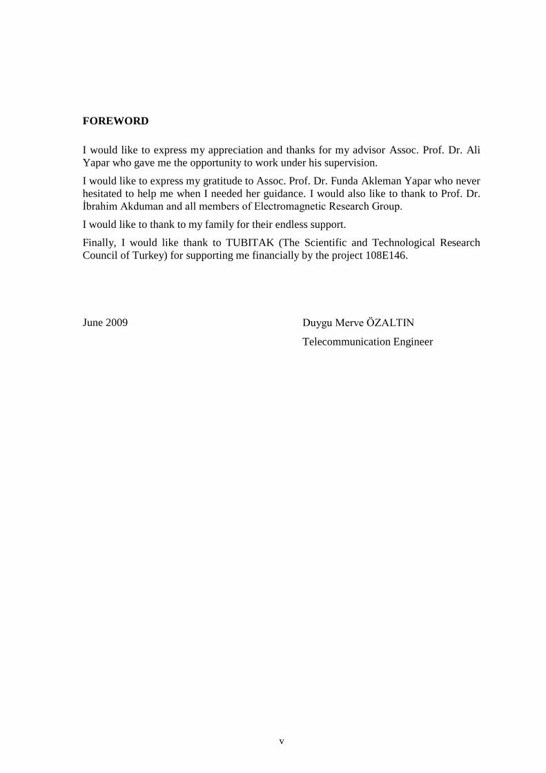
2.2 Dyadic Green’s Function for Rectangular Waveguide
The dyadic Green’s function of the electric type for rectangular waveguide is given
below (Wang, Tai).
0
0
2
1( , ) ( , ) ( )z zG r r G r r e e r r
k (2.3)
In this equation, ( , , )r x y z and ( , , )r x y z represents observation and source
points respectively. ze is the unit vector for z direction and ( )r r is three-
dimensional Dirac delta function. 0 ( , )G r r is defined below.
7
0 0 0
| |
0 0 0 020 00
0 0 0
( , )2
mn
xx x x xy x y xz x z
ik z zm nyx y x yy y y yz y z
m n mn
zx z x zy z y zz z z
G e e G e e G e ei
G r r e G e e G e e G e eabk k
G e e G e e G e e
(2.4)
2 2
00 [ ( ) ]cos cos sin sinxx
m m x m x n y n yG k
a a a b b
(2.5)
0 ( )( )cos sin sin cosxy
m n m x m x n y n yG
a b a a b b
(2.6)
0 ( )cos sin sin sin ,mnxz
m m x m x n y n yG ik z z
a a a b b
(2.7)
0 ( )( )sin cos cos sinyx
m n m x m x n y n yG
a b a a b b
(2.8)
2 2
00 [ ( ) ]sin sin cos cosyy
n m x m x n y n yG k
b a a b b
(2.9)
0 ( )sin sin cos sin ,mnyz
n m x m x n y n yG ik z z
b a a b b
(2.10)
0 ( )sin cos sin sin ,mnzx
m m x m x n y n yG ik z z
a a a b b
(2.11)
0 ( )sin sin sin cos ,mnzy
n m x m x n y n yG ik z z
b a a b b
(2.12)
2 2
0 [( ) ( ) ]sin sin sin sinzz
m n m x m x n y n yG
a b a a b b
(2.13)
The equations below are used in Green’s function.
1, 0
0n
n
n
(2.14)
2 20mn ck k k (2.15)
2 2 2( ) ( )c
m nk
a b
(2.16)

8
If observation and source points are not close to each other, convergence of series in
the Green’s function is achieved. Otherwise, convergence problem occurs and this
problem creates great difficulty in computation. To solve this convergence problem,
partial summation technique is used. In this method, slowly convergent series are
replaced with the series which have analytical expressions. With the help of partial
summation technique, it is possible to take integral of the dyadic Green’s function for
all cells (Wang).
2.3 Method of Moments
Solution by Method of Moments (MoM) for electromagnetic problems can be
achieved by following the steps below.
1. Deriving integral equation
2. Using basis functions and weighting functions to convert integral equation
into matrix equation
3. Evaluating matrix elements
4. Solving matrix equation and obtaining parameters that are to be determined.
MoM solution of the described problem which involves an inhomogeneous material
loaded in rectangular waveguide is handled by J. J. H. Wang. This approach is
described below.
Let the volume V of the dielectric material which is loaded in the rectangular
waveguide is divided into L equal rectangular sided cells which have dimensions Δx,
Δy, Δz in x,y,z directions respectively. The electric field is assumed to be uniform
inside one cell and is taken as E(rl) for lth cell where rl represents lth cell center. The
equivalent current can be expressed as linear combinations of basis functions ( )klB r .
3
1 1
( ) ( )L
k kl l
l k
J r J B r
(2.17)
The basis function is defined as
ˆ( ) ( )lk
kl
B r u P r , k=1,2,3 or x,y,z (2.18)
k index denotes x,y,z coordinates and ˆku is the unit vector in specified direction and
( )lP r is defined as follows.

9
1( )
0
ll r VP r
else
(2.19)
The weighting function ( )pqW r is taken as follows:
ˆ( ) ( )pq q pW r r r u , p=1,2,3 (2.20)
The scalar product is defined between f and g as,
, .V
f g f gdv (2.21)
After basis and weighting functions are chosen, the equivalent current which is
defined in terms of basis functions linear combination is substituted into the main
integral equation and then scalar product is performed on the resulting equation with
the weighting function ( )pqW r for p=1,2,3 and q=1,2,…,L. After this moment
generating procedure, the following equations are obtained (Wang).
3
1 1
Lk pq pql kl
k l
J A C
p=1,2,3 ; q=1,2,3,…,L (2.22)
pqC and
pqklA are expressed as follows:
( )pq iqC E r (2.23)
0
0
3 3.
( ) ( )
l p k pqpq pk k
kl lq
q q
A j Qj r r
(2.24)
In this equation, p
k is Kronecker delta which is takes the value 1 when p=q and 0
otherwise.
0 ( , ) '
l
pk pklq
V
Q G r r dV
(2.25)
0 ( , )pkG r r is the (p,k) component of the dyad 0 ( , )G r r .
The integration in the pklqQ definition can be reformed as,
0 02
0 02
pk pkn mmnlq
n m mn
jQ IQF
abk k
(2.26)
pk
mnF and Q is defined as follows:

10
0( , ) .mn q ljk z zpk pk
mn eF the m n th term of G e
(2.27)
4sin sin
2 2
l ln X m YabQ
n m a b
(2.28)
The definition of I varies depending on pk index due to the dyad expression.
For (p,k) = { (1,3), (2,3), (3,1), (3,2) } where (1,2,3) refers to the coordinates (x,y,z)
respectively, I can be expressed as follows,
/2
2sin / 2
2
2sin
mn q l
q l
mn l
jk z z mn lq l l
mn
mn
mn
jk z
k ze z z z
kI
e k z z elsek
(2.29)
For other p,k indices, I is expressed as follows:
/22cos 1 / 2 / 2
2sin / 2
q l
q
l
mn ql l l l
mn
z z
mn
mn
mn l
mn
jk z
jk
k z z e z z z z zjk
I
k z e elsek
(2.30)
The matrix element pqklA has double infinite series and it does not converge rapidly
unless |zq-zl| is large. In the case that p=q, cells are diagonal matrix elements |zq-zl|=0
and convergence of the series is extremely slow.To solve this computational
problem, partial summation technique is used. By using this technique, matrix
element of double infinite series can be transformed into single infinite series or in
some cases it can be transformed into an expression of closed form which can be
truncated for computation (Wang). The parts of the infinite series which have terms
slowly convergent with m and n are summed by means of the following equations.
1
sin
2k
kx x
k
, 0 2x (2.31)
2 21
.sin sinh ( )
2 sinhk
k ka a x
k a a
, 2a >0 , 0 2x (2.32)
2 2
0
sin (2 1).sin
2sink
a m xk kx
k a a
, 2 (2 2)m x m , a : noninteger (2.33)

11
2 2 21
cos cosh( ) 1
2 sinh 2k
kx x
k a a a a
, 0 2x (2.34)
2 2 2
1
cos (2 1)cos 1
2 2 sink
a m xkx
k a a a a
(2.35)
2 (2 2)m x m , a : noninteger
2.4 Finite Difference Time Domain
Finite difference time domain (FDTD) is another useful and popular computational
technique which is used for electromagnetic problems. It is mainly based on second
order central difference approximantions in space and time for Maxwell’s time
dependent curl equations. Finite difference methods are known and used for many
years but it has not been used for Maxwell’s equations until Yee. In 1966, K.S.Yee
proposed FDTD algorithm which is basically finite difference method applied to
Maxwell’s equations in time domain and space. Since then, many researches are
made about this issue and Yee’s finite difference algorithm is developed. The
following section describes FDTD method for one-dimensional scalar wave function.
After this introduction, Yee’s finite difference algorithm will be described and three
dimensional FDTD analysis will be explained.
2.4.1 One-Dimensional FDTD
In an infinite homogeneous space, one-dimensional scalar wave equation can be
written as
2 22
2 2
( , ) ( , )f x t f x tc
t x
(2.36)
Solution of this equation is in a form like f(x,t)=g1(x-ct)+g2(x+ct) which represents
the superposition of forward and backward travelling waves.
If Taylor series expansion of f(x, t) is used about the point x to the point x x at a
time t, the following expressions are obtained.
2 2 3 3 4 4
2 3 4
( , ) ( , ) ( , ) ( , )( , ) ( , ) ...
2 6 24
f x t f x t x f x t x f x t xf x x t f x t x
x x x x
(2.37)

12
2 2 3 3 4 4
2 3 4
( , ) ( , ) ( , ) ( , )( , ) ( , ) ...
2 6 24
f x t f x t x f x t x f x t xf x x t f x t x
x x x x
(2.38)
These two expressions are added and the following equation is obtained.
2 4 42
2 4
( , ) ( , )( , ) ( , ) 2 ( , ) ...
12
f x t f x t xf x x t f x x t f x t x
x x
(2.39)
Second order partial derivative term can be expressed as
22
2 2
( , ) ( , ) 2 ( , ) ( , )( )
( )
f x t f x x t f x t f x x tO x
x x
(2.40)
This expression can also be written for the variable t.
22
2 2
( , ) ( , ) 2 ( , ) ( , )( )
( )
f x t f x t t f x t f x t tO t
t t
(2.41)
As it can be seen, these expressions are central difference approximation of the
second order derivative. The terms 2( )O x and 2( )O t shows the error order
and this expression is said to be second order accurate. If these two equations are
used in scalar wave equation, the following equation is obtained.
2
2
( , ) 2 ( , ) ( , )( )
( )
f x t t f x t f x t tO t
t
2 2
2
( , ) 2 ( , ) ( , )( )
( )
f x x t f x t f x x tc O x
x
(2.42)
For discrete space,
ix i x
nt n t
( , )ni i nf f x t
Discrete wave equation can be written as follows

13
1 12 2 21 1
2 2
22( ) ( )
( ) ( )
n n nn n nii i i i if f ff f f
O t c O xt x
(2.43)
Explicit time-marching solution for f can be calculated as
1 2 2 1 2 21 12
2( ) 2 ( ) ( )
( )
n n nn n nii i
i i i
f f ff c t f f O x O t
x
(2.44)
2.4.2 Three-Dimensional FDTD - Yee’s Algorithm
Finite difference method is a numerical approach which had been widely used for
many years in many areas. In 1966, this method is also applied to Maxwell’s
equations for the first time. Yee proposed a finite difference algorithm which is
applied to Maxwell’s curl equations for time domain and space. After Yee, many
researches are made and this algorithm is developed. In this section, Yee’s algorithm
is explained and three dimensional electromagnetic problems are introduced.
Maxwell’s curl equations can be expressed as
xt
HE (2.45)
xt
EH E (2.46)
In these equations, E and H are vectors and if these equations are written in scalar
form, there will be six equations. In cartesian coordinate system, these equations can
be written as
1 yx zEH E
t z y
(2.47)
1y xzH EE
t x z
(2.48)
1 yxzEEH
t y x
(2.49)
1 yx zx
HE HE
t y z
(2.50)

14
1y x zy
E H HE
t z x
(2.51)
1 y xzz
H HEE
t x y
(2.52)
To express curl equations in discrete space, below definitions are given.
ix i x , jy j y , kz k z , nt n t (2.53)
, ,( , , , ) ni j nk i j kf x y z t f (2.54)
An orthogonal grid is defined and the function f is evaluated at the vertices of the
grid. After discretizing, central difference approximation for derivatives. As an
example, the equations (2.45) and (2.48) can be expressed as
1 yx z
EH E
t z y
1/2 1/2
, 1/2, 1/2 , 1/2, 1/2 , 1/2, 1 , 1/2,
1 1 1n n n nx x y yi j k i j k i j k i j k
H H E Et z
, 1, 1/2 , , 1/2
1 1 n nz zi j k i j k
E Ey
(2.55)
1 yx zx
HE HE
t y z
1 1/2 1/2
1/2, , 1/2, , 1/2, 1/2, 1/2, 1/2,
1 1 1n n n nz zi j k i j k i j k i j kx xE E H H
t y
1/2 1/2 1/2
1/2, , 1/2 1/2, , 1/2 1/2, ,
1 1 n n ny yi j k i j k i j kxH H E
z
(2.56)
Similar operation is done for all of the equations from (2.45) to (2.50), which are the
curl equations and Yee Cell is introduced by K.Y.Yee to express these expressions
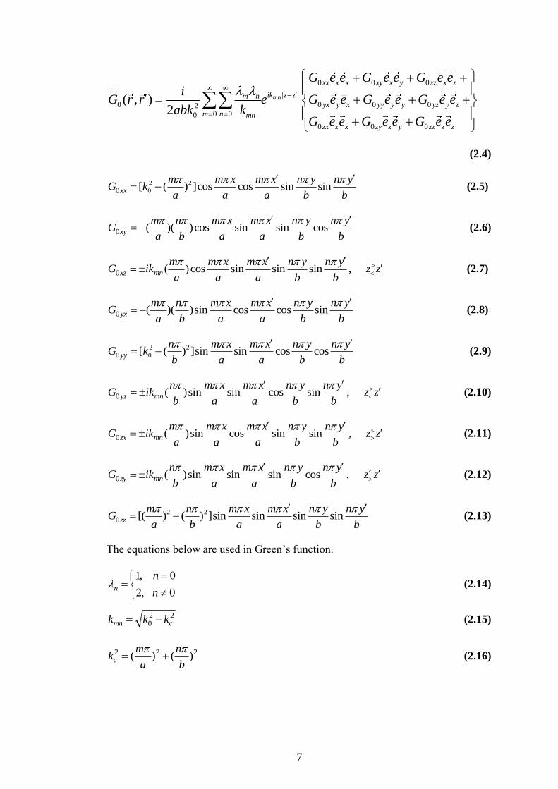
in a geometrical manner. There are two lattices called Primary Lattice and Secondary
Lattice. Assumptions about the Primary and Secondary Lattice are described below.
a) Discrete vector electric fields are parallel to and are constant along the edges
of the primary lattice.
b) Discrete vector magnetic fields are normal to and are constant throughout
each face of the primary lattice.
15
c) Discrete vector magnetic fields are parallel to and are constant along the
edges of the secondary lattice.
d) Discrete vector electric fields are normal to and are constant throughout each
face of the secondary lattice.
e) Secondary lattice edges connect the cell centers of the primary lattice.
(Gedney)
Figure 2.2 : Field components in the Yee’s lattice.
By rearranging the equation (2.53), the following equation is obtained.
1/2 1/2
, 1/2, 1/2 , 1/2, 1/2 , 1/2, 1 , 1/2,
1n n n nx x y yi j k i j k i j k i j k
tH H E E
z
, 1, 1/2 , , 1/2
1 n nz zi j k i j k
tE E
y
(2.57)
This expression and similar expressions for other components of electric and
magnetic fields refer to a part in the Yee cell. This is shown in the figure below.

16
Figure 2.3 : Field components at one side of the Yee’s lattice.
Electric and magnetic field components can be expressed as follows,
1/2 1/2
, 1/2, 1/2 , 1/2, 1/2 , 1/2, 1 , 1/2,
1n n n nx x y yi j k i j k i j k i j k
tH H E E
z
, 1, 1/2 , , 1/2
1 n nz zi j k i j k
tE E
y
(2.58)
1/2 1/2
1/2, , 1/2 1/2, , 1/2 1, , 1/2 , , 1/2
1n n n ny y z zi j k i j k i j k i j k
tH H E E
x
1/2, , 1 1/2, ,
1 n nx zi j k i j k
tE E
z
(2.59)
1/2 1/2
1/2, 1/2, 1/2, 1/2, 1/2, 1, 1/2, ,
1n n n nz z x xi j k i j k i j k i j k
tH H E E
y
1, 1/2, , 1/2,
1 n ny yi j k i j k
tE E
x
(2.60)
1 1/2 1/2
1/2, , 1/2, , 1/2, 1/2, 1/2, 1/2,
1(1 )n n n n
x x z zi j k i j k i j k i j k
tE E H H
y
1/2 1/2
1/2, , 1/2 1/2, , 1/2
1 n ny yi j k i j k
tH H
z
(2.61)
17
1 1/2 1/2
, 1/2, , 1/2, , 1/2, 1/2 , 1/2, 1/2
1(1 )n n n n
y y x xi j k i j k i j k i j k
tE E H H
z
1/2 1/2
1/2, 1/2, 1/2, 1/2,
1 n nz zi j k i j k
tH H
x
(2.62)
1 1/2 1/2
, , 1/2 , , 1/2 1/2, , 1/2 1/2, , 1/2
1(1 )n n n n
z z y yi j k i j k i j k i j k
tE E H H
x
1/2 1/2
, 1/2, 1/2 , 1/2, 1/2
1 n nx xi j k i j k
tH H
y
(2.63)
2.5 Mode Matching
Mode matching is another efficient technique which is used for boundary value
problems. This method has been applied for the solution of the scattering problems
due to discontinuities in waveguides, finlines and microstrip lines as well as analysis
of composite structures such as E-plane filters, direct-coupled cavity filters,
waveguide impedance transformers, microstrip filters and power dividers [31].
The first step of this technique is expanding the fields on both sides of discontinuity
in terms of their respective modes. After modal functions are constructed, the
problem reduces to determination of modal coefficients associated with the field
expansions at each region. Considering orthogonality of the normal modes, an
infinite set of linear equations for the unknown modal coefficients are obtained and
an approximation technique such as truncation and iteration is used in order to solve
the problem.
This method is described in detail by Mittra and Lee. For more information, please
refer to [31-32].

18
2.6 Numerical Results
In this section, numerical results are given for the solution of forward scattering
problem. The solution is obtained via three different approaches, Method of Moment,
FDTD and Mode Matching. Results show the consistence of three different and
independent methods. Two S parameters, S11 and S21, which carry the information
about reflected and transmitted fields at the input and output ports of waveguide, are
obtained at different frequencies and three techniques are compared with each other.
The first example consists of an inhomogeneous obstacle which fills the rectangular
waveguide in x, y coordinates. Waveguide cross-section dimensions are a=2,286 cm
and b=0,508 cm. The obstacle has three parts in z direction having constant relative
permittivities εr1=2 , εr2=3, εr3=2.5 in each part and each part has same length in z
direction which is 2 mm. Frequency range is between 7 GHz and 8 GHz.
Comparison of S parameters of the system is done between two different and
independent approaches which are Method of Moments and Mode Matching method.
Amplitude and phase of S11 and S21 parameters that are obtained by these two
methods are shown in the figures from figure number 2.4 to 2.7.
Figure 2.4 : Amplitude of S11 parameter for cross-sectional filled waveguide.

19
Figure 2.5 : Phase of S11 parameter for cross-sectional filled waveguide.
Figure 2.6 : Amplitude of S21 parameter for cross-sectional filled waveguide.

20
Figure 2.7 : Phase of S21 parameter for cross-sectional filled waveguide.
Another example is for an obstacle that does not fill the waveguide in any of the x, y
and z directions. Cross-section dimensions of the waveguide are a=2,2 cm and
b=1cm. Dimensions of the material are 5 mm, 5 mm, 20 mm at x ,y, z directions
respectively. Relative permittivity of the material is εr1=2. S parameters are
calculated for the frequencies from 7.2 GHz to 7.7 GHz. In this example, FDTD and
Method of Moments are used for the solution of direct problem and S parameters are
obtained. Simulation results are shown in the below figures from figure number 2.7
to 2.10.

21
Figure 2.8 : Amplitude of S11 parameter for semi-filled waveguide.
Figure 2.9 : Phase of S11 parameter for semi-filled waveguide.

22
Figure 2.10 : Amplitude of S21 parameter for semi-filled waveguide.
Figure 2.11 : Phase of S21 parameter for semi-filled waveguide.

23
3. INVERSE SCATTERING PROBLEM
In inverse scattering problems, a known incident field is applied and unknown
parameters of the scatterer are to be determined from the knowledge of scattered
field. There are several techniques to obtain constitutive parameters, size, shape,
location of the object. In this study, Contrast Source Inversion (CSI) technique is
used for the solution of inverse scattering problem. The aim is to reconstruct
complex permittivity of a dielectric material which is loaded inside a rectangular
waveguide.
3.1 Statement of the Problem
An inhomogeneous dielectric material is placed inside a rectangular waveguide as
shown in the figure (2.1) and excitation is assumed to be by dominant mode TE10.
Considering the equation (2.1), according to the location of the observation point,
two equations can be written which are called as data and object equations. When the
observation point is out of the object region Ω , data equation is expressed as
follows,
20( ) ( ) ( ; ) ( ) ( ) s sf r E r k G r r v r E r d
, r (3.1)
where ( ; )G r r is the dyadic Green’s function whose expression is given in the
previous section, Ω is the reconstruction domain, r represents observation point and
r represents source point.
( )v r is the object function to be determined which is expressed as follows
1)(
)(2
0
2
k
rkrv
(3.2)
where ( )k r represents complex wavenumber of the material.
Data equation equals to scattered field expression when the observation point is
outside of the object region.

24
When the observation point is in the object region Ω, the object equation is written as
20( ) ( ) ( ; ) ( ) ( )iE r E r k G r r v r E r d
, r (3.3)
In order to derive a solution to the equations (3.1) and (3.3), different approaches
such as Born Iterative Method, Newton Iteration Method etc. can be used. In this
study, Contrast Source Inversion (CSI) Method which gives satisfactory results for
relatively high contrast permittivity profiles is applied. This technique is described in
the following section.
3.2 Contrast Source Inversion Method
Contrast source inversion is a technique which allows to generate a priori
information about the scatterer. An important advantage of this technique is that this
method can be applied for both spatially and frequency varying incident fields (Van
den Berg, Kleinman). A simple algorithm for reconstructing unknown contrasts is
introduced by Van den Berg and Kleinman. This algorithm is a variant of the source-
type integral equation (STIE) method introduced by Habashy and modified gradient
approach.
In this method, the product of two unknowns ( )v r and ( )E r is defined as a contrast
source.
)()()( rErvrJ
(3.4)
The data and object equations are written in terms of contrast source and integral
operators GS and GD are introduced.
Data equation is expressed as
20( ) ( ; ) ( ) s Sf r k G r r J r d G J r
(3.5)
Object equation is expressed as
20( ) ( ) ( ) ( ) ( ; ) ( ) ( ) ( ) i i DJ r v r E r v r k G r r J r d v r E r G J r
(3.6)
GS and GD are integral operators for outside and inside of reconstruction domain
respectively.

25
As in other methods like modified gradient method or Van den Berg-Haak approach,
also in contrast source inversion method, a cost functional is defined and the aim is
to minimize the cost functional by simultaneously constructing sequences of contrast
sources, fields and contrasts. (Van den Berg, Kleinman). Cost functional is chosen as
the superposition of the error in data equation and the error in object equation as
2 2
2 2
M Mp p p p p p p p p
s i DS S Dp p
M Mp p p
s iS Dp p
f G J v E J v G J
F
f v E
(3.7)
where .S
and .D
denotes the norms on S and D domains respectively. The
normalization is chosen so that if J is equals to zero, both terms will be equal to 1.
The summation indicated by the index p can be over frequency or different incident
fields according to the problem. In this study, multi-frequency data is used and this
summation is over frequency.
An iterative minimization method is used which first updates J and then updates v.
Thus sequences Jp,n
and vp,n
for n=0,1,2,… are obtained in that manner.
Data and state errors are defined as
, , ,p n p n p p ns Sf G J (3.8)
, , , ,p n p n p n p nEr v J (3.9)
where
, , ,p n p i p p nDE E G J (3.10)
Suppose that , 1p nJ and , 1p nv are known and contrast source at pth iteration pJ is
calculated as follows
, , 1 , ,p n p n p n p nJ J (3.11)
where ,p n is constant and ,p n are the update directions which are functions of
position. The update directions are chosen as Polak-Ribiere conjugate gradient
directions.
,0 0p (3.12)

26
, , , 1
, , ,
, 1 , 1
,
,
p n p n p n
p n p n p nD
p n p n
D
g g gg
g g
(3.13)
where ,p ng is the gradient (Frechet derivative) of the cost functional with respect to
pJ evaluated at , 1p nJ , , 1p nv and .D
is the inner product on D. (Please refer to [4]
for details)
After the update directions are specified, the constant ,p n is determined to minimize
the cost functional. Explicit expression of ,p n is
, 1 , , 1 , , 1 ,
,
2 2
, 1
, ,p n p p n p n p n p n p p n
DSp n S D
ik k n kS D
k k
G r v G
f v E
x
122 , , 1 ,,
2 2
, 1
p n p n p p np p nDS S D
ik k n kS D
k k
v GG
f v E
(3.14)
Once ,p nJ is updated, ,p nE is determined via equations (3.17) and (3.18) as
, , 1 , ,p n p n p n p p nDE E G (3.15)
The next step is to obtain object function ,p nv that minimizes the cost functional at
each iteration. Instead of more complicated functional
2, ,
2,
Mp p n p n
Dp
D Mp p n
Dp
v E J
F
v E
(3.16)
below cost functional is used which also guarantee that the process is always error
reducing.
2, ,'
Mp p n p n
D Dp
F v E J (3.17)
This cost functional has easy implementation of a priori information or constraints on
the object function pv . In the case that there is no priori information on the object
function v, 'DF is minimized by choosing real and imaginary parts of v as

27
, ,
,
2,
Re( )M
p n p n
pr n
Mp n
p
J E
v
E
(3.18)
, ,
,
22 ,
Im( )
( )
Mp p n p n
pi n
Mp p n
p
J E
v
E
(3.19)
The object function can be expressed as
( ') ( ') ( ')p r p iv r v r i v r (3.20)
where p is the ratio between the wavenumbers for first and pth frequencies defined
as follows
0 0p
p p
k
k
(3.21)
If a priori information is available, choosing nv will be relatively simple. If either real
or imaginary part of the object function is known, it can be used in the equations
(3.25) and (3.26). For example, if 0iv , reconstruction procedure can be limited to
rv from the outset. The cost functional 'DF can be expressed in different ways
according to this information and real and imaginary part of minimizing object
function can be calculated in relatively simple way. For more information please
refer to [4].
The last thing to be mentioned about this algorithm is the choice of starting values of
contrast source ,0pJ . It is obvious that initial value can not be ,0 0pJ because
,0 ,0 0r iv v and the cost functional is undefined for n=1. Therefore, starting values
are chosen as the values obtained by backpropagation (Van den Berg, Kleinman).
Initial value of contrast source is expressed as
*
*
*
2
,0
2
p pSp p pD
Sp p pS S S
G fG f
G G fJ (3.22)
In this method, regularization is not required because of the regularization in
conjugate gradient approach.
28
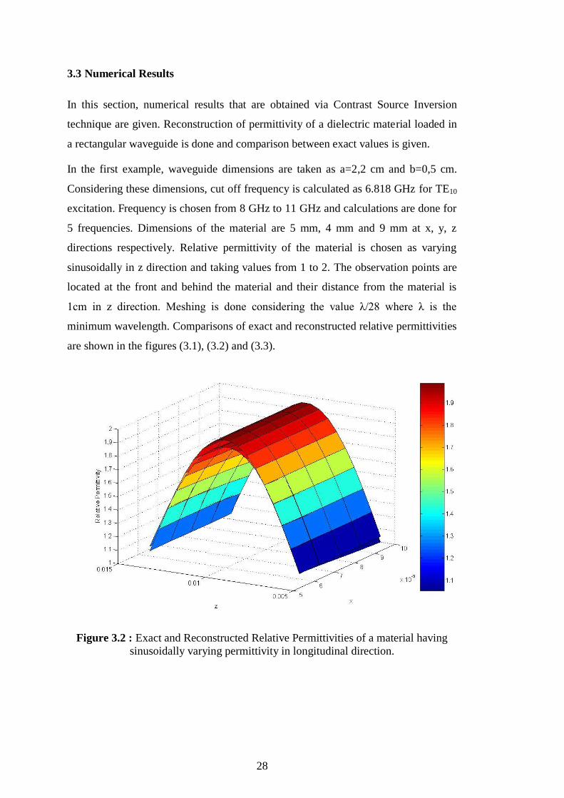
3.3 Numerical Results
In this section, numerical results that are obtained via Contrast Source Inversion
technique are given. Reconstruction of permittivity of a dielectric material loaded in
a rectangular waveguide is done and comparison between exact values is given.
In the first example, waveguide dimensions are taken as a=2,2 cm and b=0,5 cm.
Considering these dimensions, cut off frequency is calculated as 6.818 GHz for TE10
excitation. Frequency is chosen from 8 GHz to 11 GHz and calculations are done for
5 frequencies. Dimensions of the material are 5 mm, 4 mm and 9 mm at x, y, z
directions respectively. Relative permittivity of the material is chosen as varying
sinusoidally in z direction and taking values from 1 to 2. The observation points are
located at the front and behind the material and their distance from the material is
1cm in z direction. Meshing is done considering the value λ/28 where λ is the
minimum wavelength. Comparisons of exact and reconstructed relative permittivities
are shown in the figures (3.1), (3.2) and (3.3).
Figure 3.2 : Exact and Reconstructed Relative Permittivities of a material having
sinusoidally varying permittivity in longitudinal direction.

29
Figure 3.2 : Exact and Reconstructed Relative Permittivities – Cross section view.
Figure 3.3 : Exact and Reconstructed Relative Permittivities while scanning the
mesh points.

30
In the second example, waveguide dimensions and frequency is chosen same
as the first example. Object dimensions are 3 mm, 3 mm and 10 mm at x, y, z
directions respectively. Relative permittivity of the object equals to 2 from 5
mm to 9 mm and equals to 2.5 from 9 mm to 15 mm in z direction.
Observation points are the same as in the first example. Figure (3.4) shows
exact relative permittivity and figure (3.5) represents reconstructed relative
permittivity for iteration number 6000. Figure (3.6) illustrates the effect of
iteration number and comparison between 600 and 6000 is shown.
Figure 3.4 : Exact Relative Permittivity of a material having two constant
values in longitudinal direction.

31
Figure 3.5 : Reconstructed Relative Permittivity of a material having two constant
values in longitudinal direction.
Figure 3.6 : Comparison of Reconstructed Relative Permittivities for Different
numbers of iteration.
32
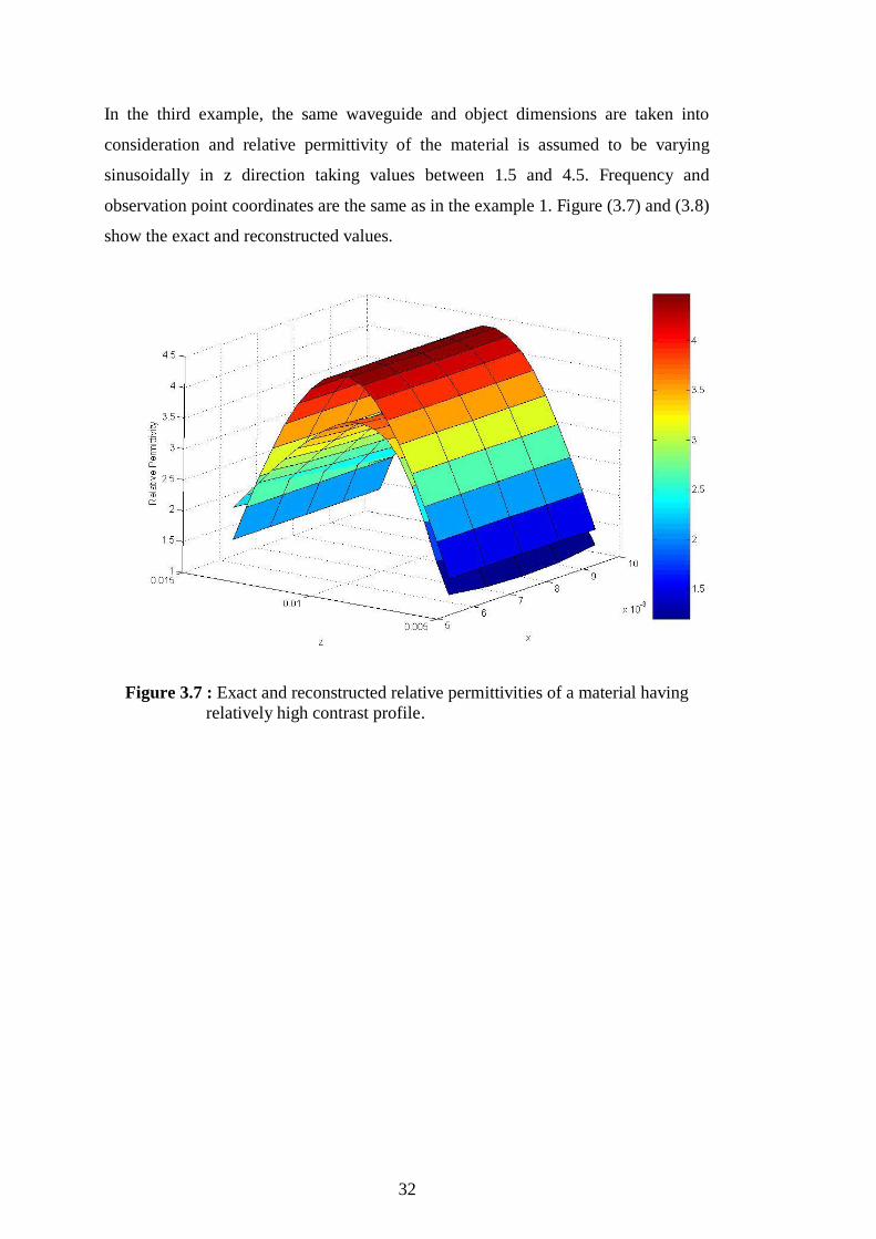
In the third example, the same waveguide and object dimensions are taken into
consideration and relative permittivity of the material is assumed to be varying
sinusoidally in z direction taking values between 1.5 and 4.5. Frequency and
observation point coordinates are the same as in the example 1. Figure (3.7) and (3.8)
show the exact and reconstructed values.
Figure 3.7 : Exact and reconstructed relative permittivities of a material having
relatively high contrast profile.

33
Figure 3.8 : Exact and reconstructed relative permittivities – cross section
view.

34

35
4. CONCLUSION AND RECOMMENDATIONS
In this study, an inverse scattering problem whose aim is to reconstruct unknown
permittivity of an inhomogeneous dielectric material which is placed in a rectangular
waveguide is presented. Three dimensional solution of this problem is obtained via
the Contrast Source Inversion (CSI) technique. Firstly, MoM, FDTD and Mode
Matching techniques which are numerical methods used for the solution of the direct
problem are introduced and validity of these three independent methods is shown by
numerical examples. Secondly, the inverse scattering problem is taken into
consideration and by using scattered field data which is obtained from the solution of
forward scattering problem, the unknown dielectric constant is reconstructed via CSI
technique. Satisfactory numerical results are obtained and given in the third section.
Meshing is generally done by choosing cell dimensions of λ/28. As higher
frequencies were included, the quality of reconstructions increased but calculation
time is increased too. As expected, for permittivities having low contrast profiles,
reconstruction is quite accurate. The numerical results including the materials whose
permittivities are sinusoidally and step varying are given in the third section.
It can be seen that the CSI method is an efficient technique that generates satisfactory
results in three-dimensional scattering problems including inhomogeneous materials
loaded in rectangular waveguides. Future studies will be about validation of this
approach with measurement data.

36

37
REFERENCES
[1] van den Berg, P. M. and Kleinman, R. E., 1997. A Contrast Source Inversion
Method. Inverse Problems 13 (1997) 1607-1620.
[2] Abubakar A. and van den Berg, P. M., 2002. The Contrast Source Inversion
Method for Location and Shape Reconstructions. Inverse Problems 18
(2002) 495-510.
[3] Akleman, F., 2008. Reconstruction of Complex Permittivity of a Longitudinally
Inhomogeneous Material Loaded in a Rectangular Waveguide. IEEE
Microwave and Wireless Components Letters, Vol.18, No.3.
[4] Haak K. F. I., van den Berg, P. M. and Kleinman R. E., 1998. Contrast Source
Inversion Method Using Multi-Frequency Data. Antennas and
Propagation Society International Symposium. IEEE Vol.2, Issues 21-
26.
[5] Wang, J. J. H., 1978. Analysis of a Three-Dimensional Arbitrarily Shaped
Dielectric or Biological Body Inside a Rectangular Waveguide. IEEE
Transactions on Microwave Theory and Techniques, Vol. MTT-26,
No.7.
[6] Harrington R. F., 1968. Field Computation by Moment Methods. New York,
Macmillan.
[7] Gedney, S. D., 2003. Computational Electromagnetics: The Finite Difference
Time Domain. Course notes.
[8] Umashankar, K. and Taflove, A., 1993. Computational Electromagnetics.
Artech House, Boston, London. ISBN 0-89006-599-3.
[9] Tai C. T., 1973. On the Eigenfunction Expansion of Dyadic Green’s Function.
Proceedings of the IEEE.
[10] Rahmat-Samii Y., 1975. On the Question of Computation of the Dyadic
Green’s Function at the Source Region in Waveguides and Cavities.
IEEE Transactions on Microwave Theory and Techniques.
[11] Mosig, J. R. and Melcon A. A., 2002. The Summation-by-Parts Algorithm - A
New Efficient Technique for Rapid Calculation of Certain Series
Arising in Shielded Planar Structures. IEEE Transactions on
Microwave Theory and Techniques, Vol. 50, No.1.
[12] Mittra, R., Hou Y.-L., and Jamnejad, V., 1980. Analysis of Open Dielectric
Waveguides Using Mode-Matching Technique and Variational
Methods. IEEE Transactions on Microwave Theory and Techniques,
Vol. MTT-28, No.1.

38
[13] Rozzi, T., Moglie, F., Morini, A., Gulloch W. and Politi M., 1992. Accurate
Full Band Equivalent Circuits of Inductive Posts in Rectangular
Waveguide. IEEE Transactions on Microwave Theory and
Techniques, Vol.40, No.5.
[14] Liang, Ji. F., Liang, X. P., Zaki K. A. and Atia A. E., 1994. Dual-Mode
Dielectric or Air-Filled Rectangular Waveguide Filters. IEEE
Transactions on Microwave Theory and Techniques, Vol.42, No.7.
[15] Cameron, R. J., Yu, M. and Wang Y., 2005. Direct Coupled Microwave
Filters With Single and Dual Stopbands. IEEE Transactions on
Microwave Theory and Techniques, Vol.53, No.11.
[16] Ishimaru, A., 1991. Electromagnetic Wave Propagation, Radiation and
Scattering. Prentice-Hall, Englewood Cliffs, New Jersey. ISBN 0-13-
249053-6.
[17] Baginski M. E., Faircloth, D. L. and Deshpande M. D., 2005. Comparison of
Two Optimization Techniques for the Estimation of Complex
Permittivities of Multilayered Structures using Waveguide
Measurments. IEEE Transactions on Microwave Theory and
Techniques, Vol. 53, No.10.
[18] Faircloth, D. L., Baginski M. E. and Wentworth S. M., 2006. Complex
Permittivity and Permeability Extraction for Multilayered Samples
using S-parameter Waveguide Measurements. IEEE Transactions on
Microwave Theory and Techniques, Vol. 54, No.3.
[19] Wang, J. J. H. and Dubberley J. R., 1989. Computation of Fields in an
Arbitrarily Shaped Heterogeneous Dielectric or Biological Body by an
Iterative Conjugate Gradient Method. IEEE Transactions on
Microwave Theory and Techniques, Vol.37, No.7.
[20] Bhattacharyya A. K., 2003. On the Convergence of MoM and Mode Matching
Solutions for Finite Array and Waveguide Problems. IEEE
Transactions on Antennas and Propagation, Vol. 51, No.7.
[21] Bondeson A., Rylander T. and Ingelström P., 2005. Computational
Electromagnetics: Texts in Applied Mathematics. New York, N.Y.,
Springer. ISBN 0387261583.
[22] Catapano I., Crocco L., D’Urso M. and Isertia T., 2006. A Novel Effective
Model for Solving 3-D Nonlinear Inverse Scattering Problems in
Lossy Scenarios. IEEE Geoscience and Remote Sensing Letters,Vol.
3, No.3.
[23] Sadiku, M. N. O., 2001. Numerical Techniques in Electromagnetics. CRC
Press, Second Edition. ISBN 0-8493-1395-3.
[24] Semenov S. Y., Bulyshev A. E., Abubakar A., Posukh V. G., Sizov Y. E.,
Scuvorov A. E., van den Berg, P. M. and Williams T.C., 2005.
Microwave-Tomographic Imaging of High Dielectric-Contrast
Objects Using Different Image-Reconstruction Approaches. IEEE
Transactions on Microwave Theory and Techniques, Vol. 53, No.7.

39
[25] Tsang, L., Kong J. A. and Ding K-H., 2000. Scattering of Electromagnetic
Waves: Theories and Applications. A Wiley-Interscience Publication.
ISBN 0-471-38799-7.
[26] Zhou, Pei-bai, 1993: Numerical Analysis of Electromagnetic Fields. Springer-
Verlag Berlin Heidelberg. ISBN 3-540-54722-3.
[27] Mostafavi M. and, Mittra, R., 1972. Remote probing of inhomogeneous media
using parameter optimization techniques. Radio Sci., Vol. 7 , No.12.
[28] Jaggard, D. and Frangos, P., 1987. The electromagnetic inverse scattering
problem for layered dispersionless dielectrics. IEEE Transactions on
Antennas and Propagation, Vol. AP-35.
[29] Bolomey, J. Ch., Lesselier D. and Peronnet G., 1982. Practical problems in
the time domain probing of lossy dielectric media. IEEE Transactions
on Antennas and Propagation, Vol. AP-30.
[30] Frangos, P. and Jaggard, D., 1987. The reconstruction of stratified dielectric
profiles using successive approximations. IEEE Transactions on
Antennas and Propagation, Vol. AP-35.
[31] Itoh, T. ed., 1989. Numerical Techniques for Microwave and Millimeter-Wave
Passive Structures. New York, Wiley.
[32] Peterson, A. F., Ray S. L. and Mittra R., 1998. Computational Methods for
Electromagnetics. New York, IEEE Press.

40

41
BIOGRAPHY
Duygu Merve Özaltın was born in Kocaeli, Turkey in 1986. She received B.Sc.
degree in Telecommunication Engineering from İstanbul Technical University in
2007. She is currently working toward the M.Sc. degree in Telecommunication
Engineering Program of Institute of Science and Technology at İstanbul Technical
University.

42