GSI Conversion Equations and Indirect Estimates of JRC and JCS Values -

Applicabitily for the Conditions of the ONKALO Facility

Wo

rk

ing

Re

po

rt 2

01

7-0

2 •

Ge

oc

he

mic

al a

nd

Ph

ys

ica

l Pro

pe

rties

an

d in

Situ

Dis

tribu

tion

Co

effic

ien

ts o

f the

De

ep

So

il Pits

OL-K

K25 A

ND

OL-K

K26 a

t Olk

iluoto

POSIVA OY

Olki luoto

FI-27160 EURAJOKI, F INLAND

Phone (02) 8372 31 (nat. ) , (+358-2-) 8372 31 ( int. )

Fax (02) 8372 3809 (nat. ) , (+358-2-) 8372 3809 ( int. )

September 2018

Working Report 2017-04

Paula Salminen, Ulf L indfors, Sophie Haapalehto

September 2018

Working Reports contain information on work in progress

or pending completion.

Paula Salminen

Pöyry Finland Oy

Ulf L indfors

I tasca Consult ing AB

Sophie Haapalehto

Posiva Oy

Working Report 2017-04

GSI Conversion Equations and Indirect Estimates of JRC and JCS Values -

Applicabitily for the Conditions of the ONKALO Facility

GSI CONVERSION EQUATIONS AND INDIRECT ESTIMATES OF JRC AND JCS VALUES – APPLICABILITY FOR THE CONDITIONS OF THE ONKALO FACILITY

ABSTRACT

This report provides results from a small-scale mapping campaign, which was conducted in ONKALO. The purpose of this study was to investigate the applicability of indirect ways to determine the Geological Strength Index (GSI) values for the brittle deformation zones and the Joint Roughness Coefficient (JRC) and Joint wall Compressive Strength (JCS) values for the fractures in the ONKALO conditions. Previously, GSI and JRC values have not been mapped at all from ONKALO tunnels and JCS values have not either been systematically mapped from ONKALO. Instead, they have been estimated indirectly from other mapped parameters.

Obtaining GSI values is important for the quantitative parametrization of the brittle deformation zones. GSI value is used as an input parameter for Hoek-Brown failure criterion (Hoek et al. 2002). For the parametrization of the brittle deformation zones intersecting ONKALO, GSI values corresponding to the core zones of the brittle deformation zones have been derived from mapped Q´ parameters from the drill core, tunnel and shaft intersections (e.g. Salminen 2018, Salminen et al. 2018).

JRC and JCS values are used for the quantitative characterization of discontinuities within the rock mass (Barton-Bandis joint criterion; Barton & Bandis 1982, Barton & Choubey 1977). Salminen et al. (2018) provided indirect estimates of JRC and JCS values for fractures in the area of entire ONKALO facility (outside of the brittle deformation zone intersections).

In this study, GSI values were mapped from several pilot hole and tunnel sections within brittle deformation zone intersections in ONKALO. A range of GSI values was obtained for each mapped section – sometimes there were even two possible ranges, depending on the observation scale. From these same rock sections, the Q´ parameters and the RMR89´ parameters were also mapped. GSI values were calculated from the mapped Q´ and RMR89´ parameters using three different conversion equations: (1) the ”conventional” equation connecting the Q´ value and the GSI value (Hoek et al. 1995), (2) a newer equation connecting the RQD, Jr and Ja values (three of the Q´ parameters) to the GSI value (Hoek et al. 2013), and (3) another new equation connecting the JCond89 and RQD values (two of the RMR89

´ parameters) to the GSI value (Hoek et al. 2013). The calculated GSI values were compared to the mapped GSI values. In the case of the studied tunnel sections, the new equation (2) most often provided GSI values closest to the mapped GSI values. In the case of pilot holes, the conventional equation (1) most often provided the best compatibility, but the new equation (2) also gave GSI values close to the mapped ones. For the conditions of ONKALO in general, based on this study, Equation (2) is recommended to be used when deriving GSI values from other mapped parameters.

JRC and JCS values were determined from six test fractures in ONKALO. These test fractures were also mapped for other parameters, which were needed in the indirect schemes to estimate JRC and JCS values presented in the report of Salminen et al. (2018) and its synthesis report by Salminen (2018). JRC value can be estimated based on the Jr value and the associated fracture profile. JCS values can be calculated based on the ratio of the rock type specific uniaxial compressive strength (UCS) of intact rock and an ”alteration” value of the fracture. In this study, this alteration value of a fracture was estimated based on the thickness of the fracture fill and the Jr profile (fracture profile). JRC and JCS values estimated with the indirect schemes were compared to the values determined directly from the fractures.

JRC values were measured with a ”comb” (a roughness profile tool). These measurements resulted to ranges (sometimes quite wide) of JRC values. The indirectly estimated JRC values fit well within these ranges, except for one fracture. It seems that the indirectly estimated JRC values are applicable – especially when taking in account that the measured JRC values are not either accurate, single values. Note, however, that only six fractures were investigated in this study.

Schmidt hammer measurements were made for the determination of the JCS values. A rebound value (R-value) was calculated from the measurement results. The JCS value itself was determined based on the rebound value and the average density of the rock. These measured JCS values are not far away from the indirectly derived JCS values, if the inaccuracies in the determination of both types of JCS values are taken in account. So, it seems that the methodology for indirect estimation of JCS values is also applicable. However, the amount of studied fractures was small (6).

Keywords: GSI, JRC, JCS, brittle deformation zone, fracture

GSI MUUNNOS KAAVOJEN SEKÄ EPÄSUORIEN JRC JA JCS ARVIOIDEN KÄYTETTÄVYYS ONKALON OLOSUHTEISSA

TIIVISTELMÄ

Tässä raportissa esitetään ONKALOssa suoritettuun pienimuotoiseen kartoituskampanjaan liittyvät tulokset. Työn tarkoituksena oli tutkia epäsuorien GSI-, JRC- ja JCS-lukujen määritysmenetelmien soveltuvuutta ONKALOn olosuhteisiin. GSI-lukuja (Geological Strength Index, geologinen lujuusindeksi) tai JRC-lukuja (Joint Roughness Coefficient, raon karkeuskerroin) ei ole aiemmin kartoitettu ONKALOn tunneleista. Myöskään JCS-lukuja (Joint wall Compressive Strength, raon puristuslujuus) ei ole mitattu systemaattisesti tunneleista. Sen sijaan GSI-, JRC- ja JCS-luvut ovat määritetty epäsuorilla menetelmillä.

GSI-lukuja käytetään hauraiden deformaatiovyöhykkeiden kvantitatiiviseen parametrisointiin, osana Hoek-Brown -murtokriteeriä. ONKALOn hauraiden deformaatiovyöhykkeiden parametrisointia varten, GSI-luvut on määritetty muuntokaavoilla vyöhykkeiden rikkonaisimman osion (ytimen) Q´-parametreistä (esim. Salminen et al. 2018, Salminen 2018).

JRC- ja JCS-lukuja sen sijaan käytetään epäjatkuvuuspintojen kvantitatiiviseen karakterisointiin (Barton-Bandis -rakomalli; Barton & Bandis 1982, Barton & Choubey 1977). Salminen et al. (2018) määritti epäsuorilla menetelmillä arviot JRC- ja JCS-luvuista raoille koko ONKALOn alueella (hauraiden deformaatiovyöhykkeiden ulkopuolella).

Tässä tutkimuksessa GSI-luku kartoitettiin useasta kivijaksosta hauraiden deformaatiovyöhykkeiden alueella ONKALOssa, sekä pilottirei´istä että tunneleista. Jokaiselle jaksolle määritettiin GSI-lukujen jakauma – joillekin jaksolle saatiin kaksi mahdollista jakaumaa, tarkastelutasosta riippuen. Samoista jaksoista kartoitettiin myös Q´-parametrit ja RMR89´-parametrit. Niiden perusteella laskettiin GSI-luku kolmella eri muuntokaavalla: (1) ns. perinteinen kaava, joka yhdistää Q´-luvun ja GSI-luvun (Hoek et al. 1995), (2) uudempi kaava, joka yhdistää RQD-, Ja- ja Jr-luvut (kolme Q´-parametreistä) GSI-lukuun (Hoek et al. 2013), sekä (3) toinen uudempi kaava, joka yhdistää JCond89 ja RQD -luvut (kaksi RMR89´-parametreistä) GSI-lukuun (Hoek et al. 2013). Eri kaavoilla laskettuja GSI-lukuja verrattiin kartoitettuihin lukuihin. Tutkituille tunnelileikkauksille kaava (2) tuotti selvästi parhaan vastaavuuden kartoitettujen GSI-lukujen kanssa. Pilottireikien leikkauksille ”perinteinen” kaava (1) tuotti parhaan vastaavuuden, mutta uudemman kaavan (2) avulla lasketut GSI-luvut olivat myös lähellä kartoitettuja GSI-lukuja. Yleisesti ONKALOn olosuhteisissa, tämän tutkimuksen perusteella, voidaan suositella käytettäväksi kaavaa (2) kun halutaan laskea GSI-luku muiden kartoitettujen parametrien perusteella.

JRC- ja JCS-luvut määritettiin kuudesta eri testiraosta ONKALOssa. Näistä raoista määritettiin myös useita parametreja, joita tarvittiin epäsuoriin JRC- ja JCS-lukujen määrityksiin. JRC-luvut voidaan arvioida Jr-lukujen sekä Jr-profiilien (rakoprofiilien) perusteella. JCS-luvut puolestaan voidaan laskea kivilajikohtaisen ehjän kiven puristuslujuuden (UCS, uniaxial compressive strength) ja muuttuneisuuden suhteesta (ks.

Salminen et al. 2018, Salminen 2018). Tässä tutkimuksessa kunkin raon muuttuneisuuden määrä arvioitiin raontäytteen paksuuden ja rakoprofiilin (Jr profiili) perusteella. Epäsuorilla menetelmillä määritettyjä JRC- ja JCS-lukuja verrattiin vastaavista raoista suoraan määritettyihin lukuihin.

JRC-luvut mitattiin raoista näihin mittauksiin tarkoitetulla erityisellä ”kammalla”. Näin saatiin määritettyä JRC-lukujen jakaumat kullekin raolle. Josku nämä jakaumat olivat melko suuriakin. Näihin jakaumiin epäsuoralla menetelmällä määritetyt JRC-luvut osuivat hyvin, yhtä rakoa lukuun ottamatta. Näyttäisikin, että JRC-luvut voidaan määrittää Jr-lukujen ja Jr-profiilien perusteella – etenkin kun ottaa huomioon, että myöskään raoista määritetyt JRC-luvut eivät ole tarkkoja, yksittäisiä arvoja. On kuitenkin otettava huomioon, että tutkimuksessa oli mukava vain kuusi rakoa.

JCS-lukujen määritystä varten tehtiin mittauksia Schmidtin vasaralla. Mittausten perusteella laskettiin ns. R-arvot. R-arvojen ja kiven tiheyden perusteella arvioitiin varsinainen JCS-luku. Nämä mittauksiin perustuvat JCS-luvut eivät ole kaukana epäsuoralla menetelmällä määritetyistä JCS-luvuista, mikäli otetaan huomioon epätarkkuudet molempien JCS-lukujen määrityksessä. Menetelmä JCS-lukujen määrittämiseksi epäsuoralla menetelmällä näyttäisi siis myös olevan käyttökelpoinen. On silti huomioitava, että tutkittujen rakojen lukumäärä oli pieni (6).

Avainsanat: GSI, JRC, JCS, hauras deformaatiovyöhyke, rako

1

TABLE OF CONTENTS ABSTRACT TIIVISTELMÄ 1 INTRODUCTION................................................................................................... 3

1.1 The ONKALO facility and the site of Olkiluoto ................................................. 6 1.2 GSI values and the parametrization of the brittle deformation zones .............. 8 1.3 In situ stress field at Olkiluoto ....................................................................... 10 1.4 Posiva´s current mapping system ................................................................. 13

1.4.1 Tunnel mapping system ......................................................................... 13 1.4.2 Drill holes ............................................................................................... 14

1.5 Deformation zone intersections ..................................................................... 15 2 THE MAPPING CAMPAIGN ............................................................................... 17

2.1 GSI values .................................................................................................... 19 2.1.1 Demonstration tunnel 1 and the pilot hole ONK-PH17 ........................... 20 2.1.2 Demonstration tunnel 2 and the pilot hole ONK-PH16 ........................... 21 2.1.3 The pilot hole ONK-PH26 (Demonstration tunnel 3)............................... 22 2.1.4 AJYH13 ................................................................................................. 22

2.2 JRC and JCS values ..................................................................................... 24 3 THEORY AND FORMULATION BEHIND THE PARAMETERS .......................... 25

3.1 RQD (Rock Quality Designation) index ......................................................... 25 3.2 The Rock Tunnelling Quality Index Q and the modified Tunnelling Quality Index Q´ ................................................................................................................. 25

3.2.1 The mapping of the Q´ parameters during the campaign ....................... 27 3.3 The RMR89 rating system .............................................................................. 27 3.4 GSI conversion equations ............................................................................. 28 3.5 The Joint Roughness Coefficient, JRC ......................................................... 29

3.5.1 Indirect estimates .................................................................................. 29 3.5.2 Measured JRC values ........................................................................... 30

3.6 The Joint wall Compressive Strength, JCS ................................................... 30 3.6.1 Indirect estimates .................................................................................. 30 3.6.2 JCS values from Schmidt hammer measurements ................................ 32

4 RESULTS OF THE MAPPING CAMPAIGN ........................................................ 33 4.1 Brittle deformation zone intersections ........................................................... 33

4.1.1 Orientations of the main fault zones ....................................................... 33 4.1.2 Q´ parameters ....................................................................................... 34 4.1.3 RMR89´ ratings ....................................................................................... 37 4.1.4 GSI values ............................................................................................. 40

4.2 JRC and JCS values ..................................................................................... 43

2

4.2.1 JRC values ............................................................................................ 44 4.2.2 JCS values ............................................................................................ 45

5 DISCUSSION ...................................................................................................... 47 5.1 Q´ values and RMR89´ values ....................................................................... 47 5.2 GSI values .................................................................................................... 47 5.3 JRC and JCS values ..................................................................................... 48

5.3.1 JRC values ............................................................................................ 48 5.3.2 JCS values ............................................................................................ 49

6 CONCLUSIONS .................................................................................................. 51 6.1 GSI values .................................................................................................... 51 6.2 JRC and JCS values ..................................................................................... 52

7 REFERENCES ................................................................................................... 53 8 APPENDICES ..................................................................................................... 57

3

1 INTRODUCTION

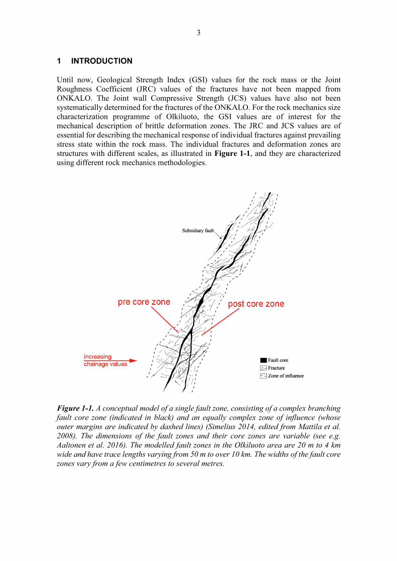
Until now, Geological Strength Index (GSI) values for the rock mass or the Joint Roughness Coefficient (JRC) values of the fractures have not been mapped from ONKALO. The Joint wall Compressive Strength (JCS) values have also not been systematically determined for the fractures of the ONKALO. For the rock mechanics size characterization programme of Olkiluoto, the GSI values are of interest for the mechanical description of brittle deformation zones. The JRC and JCS values are of essential for describing the mechanical response of individual fractures against prevailing stress state within the rock mass. The individual fractures and deformation zones are structures with different scales, as illustrated in Figure 1-1, and they are characterized using different rock mechanics methodologies.

Figure 1-1. A conceptual model of a single fault zone, consisting of a complex branching fault core zone (indicated in black) and an equally complex zone of influence (whose outer margins are indicated by dashed lines) (Simelius 2014, edited from Mattila et al. 2008). The dimensions of the fault zones and their core zones are variable (see e.g. Aaltonen et al. 2016). The modelled fault zones in the Olkiluoto area are 20 m to 4 km wide and have trace lengths varying from 50 m to over 10 km. The widths of the fault core zones vary from a few centimetres to several metres.

4

This study is linked to the parametrization work of brittle deformation zones and fractures of ONKALO. The results of the new, revised parametrization are published in the report of Salminen et al. (2018) and its synthesis report by Salminen (2018). Results of earlier parametrization works have been published in the working reports by Kuula (2010), Mönkkönen et al. (2012), Simelius (2014) and Salminen & Simelius (2016). In the parametrization work, GSI values have been used in the characterization of the brittle deformation zones. These GSI values have been derived from Q´ mapping data of the fault core zones, using different GSI conversion equations. More background information about the GSI values and the parametrization of the brittle deformation zones is given in Chapter 1.2.

In this study, the applicability and the accuracy of the different GSI conversion equations for the conditions of the ONKALO facility was tested. GSI values were mapped from the several deformation zone intersections of ONKALO. These mapped GSI values were compared to estimated GSI values, which were derived from other parameters simultaneously mapped from the same study sites. The motivation for this testing of the applicability of the different GSI conversion equations comes from the inconsistency between (i) the rock mechanics parametrization of fractures and deformation zones (Kuula 2010) and (ii) subsequent modelling of stress and geology interaction (Valli et al. 2011), as noted in the technical review of Chapman et al. (2015). The stress state of the Olkiluoto site is described in Chapter 1.3.

In addition to the parameters for the Q´ value, the parameters for the RMR89´ value were also mapped from the studied deformation zone intersections. Accordingly, this work provides also a good reference for the comparing Q´ and RMR89´ values in the conditions of ONKALO, presented from Chapter 2 onwards.

Hudson et al. (2008) suggest six different methods for the characterization of the brittle deformation zones. These are (i) direct measurement in the field (using a pressuremeter or a flatjack), (ii) indirect measurements, (iii) rock mass classification, (iv) analytical formulae, (v) numerical modelling (e.g. 3DEC), and (vi) back analysis from in situ displacement measurements. In this report, both the indirect methods as well as rock mass classification have been used.

JRC and JCS values are used for the characterizing discontinuities. They are input parameters for Barton-Bandis joint model (Barton & Bandis 1982, Barton & Choubey 1977). Salminen et al. (2018) provided indirect estimates of JRC and JCS values for fractures in the area of entire ONKALO facility (outside of the brittle deformation zone intersections). Those JRC and JCS estimates were further used in the calculations of stiffness parameters, instantaneous cohesions and friction angles, and peak dilation angles.

In this study, JRC and JCS values were measured from six test fractures in ONKALO to be able to investigate the applicability of the indirect ways to estimate these values. All necessary parameters for the indirect estimates of the JRC and JCS values were also mapped from the same test fractures. JRC values can be indirectly estimated based on other fracture descriptive parameters (see Chapter 3.5.1). JCS values can be estimated by combining the geological and geotechnical knowledge of the host rock with individual fracture descriptive parameters (for more details, see Chapter 3.6.1). The indirectly

5

derived JRC and JCS values were compared to the measured values. Based on the results of this study, it was possible to assess the applicability of the indirect JRC and JCS determination schemes applied in the work of Salminen et al. (2018) for the fractures of ONKALO.

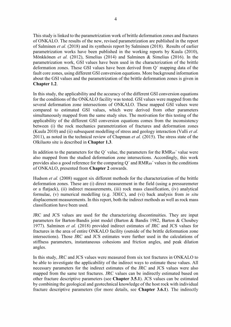
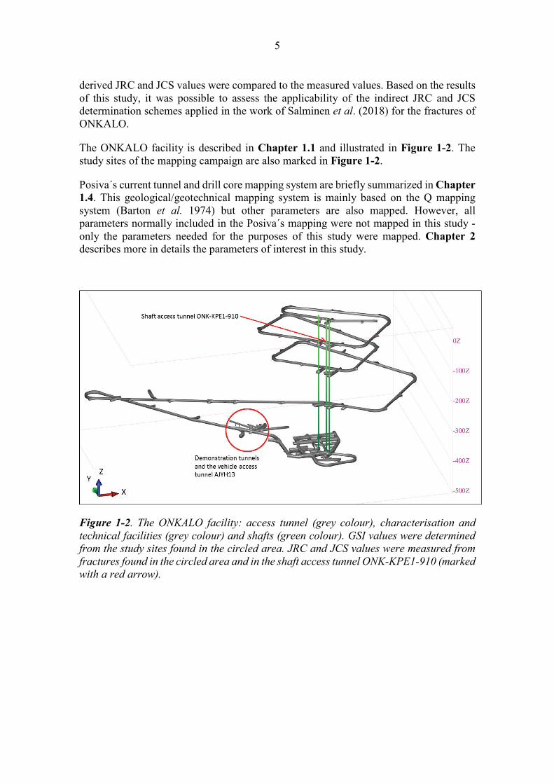
The ONKALO facility is described in Chapter 1.1 and illustrated in Figure 1-2. The study sites of the mapping campaign are also marked in Figure 1-2.

Posiva´s current tunnel and drill core mapping system are briefly summarized in Chapter 1.4. This geological/geotechnical mapping system is mainly based on the Q mapping system (Barton et al. 1974) but other parameters are also mapped. However, all parameters normally included in the Posiva´s mapping were not mapped in this study - only the parameters needed for the purposes of this study were mapped. Chapter 2 describes more in details the parameters of interest in this study.

Figure 1-2. The ONKALO facility: access tunnel (grey colour), characterisation and technical facilities (grey colour) and shafts (green colour). GSI values were determined from the study sites found in the circled area. JRC and JCS values were measured from fractures found in the circled area and in the shaft access tunnel ONK-KPE1-910 (marked with a red arrow).

6

1.1 The ONKALO facility and the site of Olkiluoto

The ONKALO facility is located next to the nuclear power plants of the Olkiluoto island, in the western Finland by the Baltic Sea. The island of Olkiluoto belongs to the municipality of Eurajoki.

ONKALO is an underground rock characterisation facility, which is one element of the site investigations conducted at Olkiluoto. The purpose of the investigations conducted by Posiva Oy is to prepare the construction of the final disposal facility of high active nuclear waste. Research aiming for detailed site characterization has been conducted in ONKALO since 2004, when the construction of ONKALO was started. The bedrock of ONKALO has been studied for investigation of geology, geophysics, hydrology and geochemistry. ONKALO also provides an opportunity to develop excavation and final disposal techniques in realistic conditions. In future, ONKALO will also be utilised for construction and will ultimately become a part of the final disposal facility.

The ONKALO facility consists of one access tunnel, characterisation and technical facilities and three shafts. The access tunnel of ONKALO reaches the depth of -455 m. The shafts include a personnel shaft, an exhaust air shaft and an inlet air shaft.

Based on the report of Aaltonen et al. (2016), a short description of the bedrock is given here. The bedrock of Olkiluoto mainly consists of variably migmatised supracrustal high-grade metamorphic rocks (e.g. different types of gneisses). These are intruded by granitic-tonalitic plutonic rocks and granitic pegmatoids. In addition, diabase dikes are intruding the supracrustal rocks. More detailed description of the lithology can be found in Aaltonen et al. (2016).

The bedrock of Olkiluoto has also been imposed to high-grade metamorphism, retrogressive metamorphism as well as surface weathering. Different episodes of hydrothermal alteration have also been documented in the Olkiluoto area. Four stages of ductile deformation (D1 to D4) have been identified at Olkiluoto site and are connected with the formation of migmatites. Brittle deformation has affected the Olkiluoto bedrock for a long time during the cooling periods of the bedrock (Aaltonen et al. 2016). More details of the deformation zone intersections (in the tunnels, shafts and drill cores) are given in Chapter 1.5.

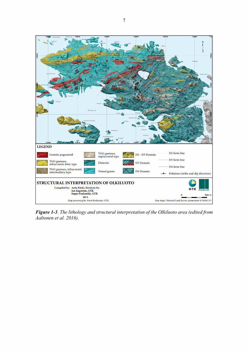
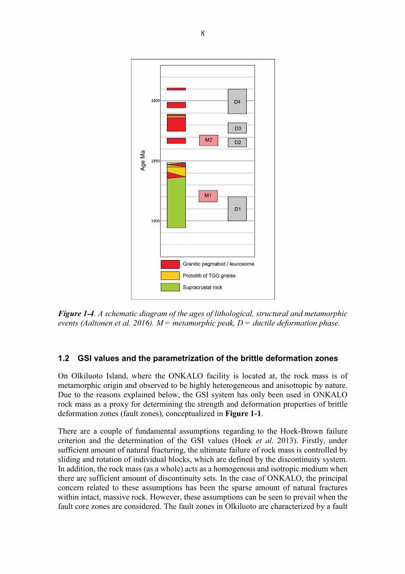
The lithology and structural interpretation of the Olkiluoto area is illustrated in Figure 1-3. A schematic presentation of the ages of lithological, structural and metamorphic events is shown in Figure 1-4.

7

Figure 1-3. The lithology and structural interpretation of the Olkiluoto area (edited from Aaltonen et al. 2016).

8

Figure 1-4. A schematic diagram of the ages of lithological, structural and metamorphic events (Aaltonen et al. 2016). M = metamorphic peak, D = ductile deformation phase.

1.2 GSI values and the parametrization of the brittle deformation zones

On Olkiluoto Island, where the ONKALO facility is located at, the rock mass is of metamorphic origin and observed to be highly heterogeneous and anisotropic by nature. Due to the reasons explained below, the GSI system has only been used in ONKALO rock mass as a proxy for determining the strength and deformation properties of brittle deformation zones (fault zones), conceptualized in Figure 1-1.

There are a couple of fundamental assumptions regarding to the Hoek-Brown failure criterion and the determination of the GSI values (Hoek et al. 2013). Firstly, under sufficient amount of natural fracturing, the ultimate failure of rock mass is controlled by sliding and rotation of individual blocks, which are defined by the discontinuity system. In addition, the rock mass (as a whole) acts as a homogenous and isotropic medium when there are sufficient amount of discontinuity sets. In the case of ONKALO, the principal concern related to these assumptions has been the sparse amount of natural fractures within intact, massive rock. However, these assumptions can be seen to prevail when the fault core zones are considered. The fault zones in Olkiluoto are characterized by a fault

9

core, surrounded with a zone of influence containing highly increased intensity of fracturing along with distance approaching the fault core. Some narrow core zones may not fulfil the assumptions, because they may be tectonically pre-sheared. In addition, the fulfilment of the assumptions is also a scale issue: when the scale increases, more joint sets are probably included and the rock mass can fulfil the basic assumptions. More discussion about the fulfilment of the fundamental assumptions (in the case of the fault core zones of ONKALO) is presented in the reports of Salminen et al. (2018) and Salminen (2018). Despite its limitations, the usage of the GSI values has still been regarded as the best available way to parametrise the brittle deformation zones of ONKALO.

A parametrization of rock mechanics properties of selected brittle fault zones of Olkiluoto was provided in the working reports of Kuula (2010), Mönkkönen et al. (2012), Simelius (2014) and Salminen & Simelius (2016). In these reports, the mapped Q´ values were converted to GSI values using the conversion equation suggested by Hoek et al. (1995), presented in Equation 4. The Q´ mapping data was obtained from the core zones (or possible core zones) of brittle deformation zone intersections in tunnels, shafts and drill cores. The derived GSI values then acted as an input values to Hoek-Brown criterion (see e.g. Hoek et al. 2002) on determining the strength and deformation properties of the mapped brittle deformation zone. In addition, a Mohr-Coulomb fit was applied for the fault core zones to obtain stiffness parameters and cohesion values for a specific range of confining stress state (see Hoek et al. 2002).

As mentioned earlier, the motivation for this study is based on the observed inconsistency between (i) the rock mechanics parametrization of fractures and brittle deformation zones (Kuula 2010) and (ii) the subsequent stress-geology modelling of Olkiluoto Island (Valli et al. 2011). Valli et al. (2011) concluded that the actual strength and deformation properties of the modelled brittle deformation zones should be significantly lower than those based on the results of Kuula (2010) - if the observed scatter in the in situ stress measurement data is to be explained by the interaction between the deformation zones and in situ stress field. The main reason for too high strength and deformation properties of the deformation zones, based on the work of Kuula (2010), is apparently due to the applied Q´- GSI conversion equation of Hoek et al. (1995).

New suggested equations connecting GSI values to the Q´ parameters (RQD, Jr and Ja) or the RMR89´ parameters (JCond89 and RQD) have emerged since 2010, notably in the research of Hoek et al. (2013). However, the application of any conversion equation relating two different mapping systems between each other should always be confirmed with an in situ mapping exercise (e.g. Hoek et al. 2013).

Within this study, the applicability three different GSI conversion equations were tested for the conditions of the ONKALO facility. These equations included the conventional equation of Hoek et al. (1995) as well as two newer equations suggested by Hoek et al. (2013).

The mapping exercise and subsequent data analysis presented in this report was conducted in conjunction with the revision of the rock mechanics mapping data analysis reported in the working report of Salminen et al. (2018) and its synthesis report by Salminen (2018). The work of Salminen et al. (2018) aims to find the correct

10

methodology for determining the stiffness and strength properties of natural fractures and brittle deformation zones in ONKALO, based on the available mapping and laboratory data of the whole site. The parametrization of the brittle deformation zones applies an alternative GSI conversion equation of Hoek et al. (2013) presented in Equation 6, instead of the conventional equation (Eq. 4) of the Hoek et al. (1995).

1.3 In situ stress field at Olkiluoto

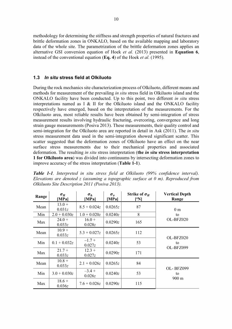
During the rock mechanics site characterization process of Olkiluoto, different means and methods for measurement of the prevailing in situ stress field in Olkiluoto island and the ONKALO facility have been conducted. Up to this point, two different in situ stress interpretations named as I & II for the Olkiluoto island and the ONKALO facility respectively have emerged, based on the interpretation of the measurements. For the Olkiluoto area, most reliable results have been obtained by semi-integration of stress measurement results involving hydraulic fracturing, overcoring, convergence and long strain gauge measurements (Posiva 2013). These measurements, their quality control and semi-integration for the Olkiluoto area are reported in detail in Ask (2011). The in situ stress measurement data used in the semi-integration showed significant scatter. This scatter suggested that the deformation zones of Olkiluoto have an effect on the near surface stress measurements due to their mechanical properties and associated deformation. The resulting in situ stress interpretation (the in situ stress interpretation 1 for Olkiluoto area) was divided into continuums by intersecting deformation zones to improve accuracy of the stress interpretation (Table 1-1).

Table 1-1. Interpreted in situ stress field at Olkiluoto (99% confidence interval). Elevations are denoted z (assuming a topographic surface at 0 m). Reproduced from Olkiluoto Site Description 2011 (Posiva 2013).

Range 𝝈𝝈𝑯𝑯 [MPa]

𝝈𝝈𝒉𝒉 [MPa]

𝝈𝝈𝒗𝒗 [MPa]

Strike of 𝝈𝝈𝑯𝑯 [oN]

Vertical Depth Range

Mean 13.0 + 0.031z 8.5 + 0.024z 0.0265z 87 0 m

to OL-BFZ020

Min 2.0 + 0.030z 1.0 + 0.020z 0.0240z 8

Max 24.0 + 0.033z

16.0 + 0.028z 0.0290z 165

Mean 10.9 + 0.033z 5.3 + 0.027z 0.0265z 112

OL-BFZ020 to

OL-BFZ099 Min 0.1 + 0.032z –1.7 +

0.027z 0.0240z 53

Max 21.7 + 0.033z

12.3 + 0.027z 0.0290z 171

Mean 10.8 + 0.033z 2.1 + 0.026z 0.0265z 84

OL- BFZ099 to

900 m Min 3.0 + 0.030z –3.4 +

0.026z 0.0240z 53

Max 18.6 + 0.036z 7.6 + 0.026z 0.0290z 115

11

The semi-integration of results from different stress measurement techniques for the Olkiluoto area yields usable mean values and variations for both the in situ stress tensor magnitude and orientation. However, for the purpose of optimised construction of a spent nuclear fuel repository and increased long term safety, more accurate model for the depth range from the brittle deformation zone OL-BFZ020 to the brittle deformation zone OL-BFZ099 was found necessary - in addition to understanding the interaction of deformation zone properties and the prevailing stress state.

The depth interval from OL-BFZ020 to OL-BFZ099 was characterized by the in situ stress measurements conducted within the ONKALO research facility located at the depth of -420 m. For the above mentioned depth interval at which the spent nuclear fuel repository level will be located at, the most reliable in situ stress measurement results have been obtained with LVDT-cell based overcoring technique as described in the report of Hakala et al. (2014). The resulting repository depth in situ stress interpretation based on the analysis of LVDT-cell measurements was named as the in situ stress interpretation 2.

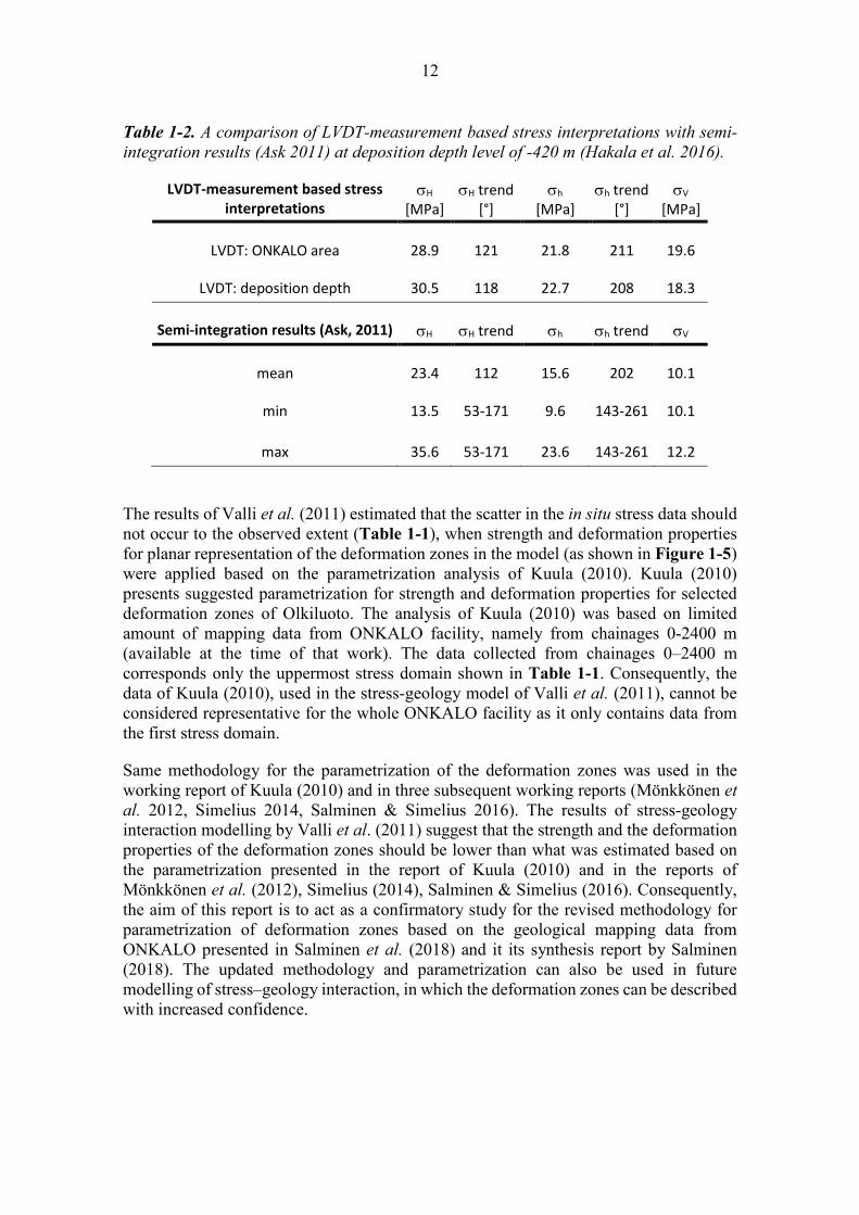
Based on the most recent analysis and quality control of LVDT-cell measurements, both the semi integration and LVDT-cell based stress interpretation corroborate each other in the repository depth of -420 m (Hakala et al. 2016). A comparison of LVDT-cell measurement based stress interpretations with semi-integration results at the level of -420 m is shown in Table 1-2.

As the LVDT-cell method is an overcoring based in situ stress measurement technique integrating over tunnel volume, it can only be performed from a pre-existing tunnel surface (Hakala et al. 2014). Consequently, its applicability is limited on detailed characterization of the two different depth levels: from the surface to OL-BFZ020, and from the OL-BFZ020 up to the maximum depth of ONKALO (around -450 m). For the improved understanding of the in situ stress state and deformation zone interaction on these two continuums, the interaction of deformation zones to the prevailing in situ stress state has been modelled by Valli et al. (2011) and subsequently in Valli et al. (2016).

12

Table 1-2. A comparison of LVDT-measurement based stress interpretations with semi-integration results (Ask 2011) at deposition depth level of -420 m (Hakala et al. 2016).

LVDT-measurement based stress interpretations

σH

[MPa]

σH trend

[°] σh

[MPa]

σh trend

[°] σV

[MPa]

LVDT: ONKALO area 28.9 121 21.8 211 19.6

LVDT: deposition depth 30.5 118 22.7 208 18.3

Semi-integration results (Ask, 2011) σH

σH trend

σh

σh trend

σV

mean 23.4 112 15.6 202 10.1

min 13.5 53-171 9.6 143-261 10.1

max 35.6 53-171 23.6 143-261 12.2

The results of Valli et al. (2011) estimated that the scatter in the in situ stress data should not occur to the observed extent (Table 1-1), when strength and deformation properties for planar representation of the deformation zones in the model (as shown in Figure 1-5) were applied based on the parametrization analysis of Kuula (2010). Kuula (2010) presents suggested parametrization for strength and deformation properties for selected deformation zones of Olkiluoto. The analysis of Kuula (2010) was based on limited amount of mapping data from ONKALO facility, namely from chainages 0-2400 m (available at the time of that work). The data collected from chainages 0–2400 m corresponds only the uppermost stress domain shown in Table 1-1. Consequently, the data of Kuula (2010), used in the stress-geology model of Valli et al. (2011), cannot be considered representative for the whole ONKALO facility as it only contains data from the first stress domain.

Same methodology for the parametrization of the deformation zones was used in the working report of Kuula (2010) and in three subsequent working reports (Mönkkönen et al. 2012, Simelius 2014, Salminen & Simelius 2016). The results of stress-geology interaction modelling by Valli et al. (2011) suggest that the strength and the deformation properties of the deformation zones should be lower than what was estimated based on the parametrization presented in the report of Kuula (2010) and in the reports of Mönkkönen et al. (2012), Simelius (2014), Salminen & Simelius (2016). Consequently, the aim of this report is to act as a confirmatory study for the revised methodology for parametrization of deformation zones based on the geological mapping data from ONKALO presented in Salminen et al. (2018) and it its synthesis report by Salminen (2018). The updated methodology and parametrization can also be used in future modelling of stress–geology interaction, in which the deformation zones can be described with increased confidence.

13

Figure 1-5. Stress-Geology model: the principle of deformation zone and repository geometry is presented in left and the 2D-cut plane of the stress evolution in right. Modified from Valli et al. (2011).

1.4 Posiva´s current mapping system

1.4.1 Tunnel mapping system

The geological/geotechnical mapping system of ONKALO tunnels has been performed in three stages: (1) the round mapping stage, (2) the systematic mapping stage, and (3) the supplementary studies. Some changes have been made for the mapping system for the lower parts of ONKALO facility. The current mapping system applied by Posiva in the construction of ONKALO is described in the report of Norokallio (2015). Previous report about the mapping guidelines was provided by Engström & Kemppainen (2008).

The round mapping stage is performed as soon as possible after the excavation of the round (usually 5 m section of the tunnel). The purpose of the round mapping stage has been to provide data to assist the geotechnical rock quality assessment of the tunnel for the ongoing excavation. Only fractures with the estimated length of ≥1 m have been mapped at this stage. Firstly, the parameters of Q classification (rock tunnelling quality index) have been obtained; rock quality designation (RQD), joint set number (Jn), joint roughness number (Jr), joint alteration number (Ja), joint water reduction numbers (Jw), and stress reduction factor (SRF). Deformation zone intersections, long fractures, main fracture orientations, rock types, grain size variations, and water leakages have also been documented at this stage. In addition, Schmidt hammer measurements on suitable fractures and various rock types have been conducted. Since 2011, the round mapping has been performed below the shotcreted roof of the previous round.

The systematic mapping stage was previously performed tens to hundreds meters behind the active excavation area. Systematic mapping included the mapping of the tunnel walls and roof in 5-10 m long sections (1-2 rounds). However, a new mapping practise was introduced for the lower parts of the ONKALO facility. After the roof of the last

14

excavated round is shotcreted, the tunnel walls and floor are cleaned. This gives an opportunity for the mapping of the tunnel floor as well. Thus, in these lower parts of ONKALO, systematic mapping has been performed in 3-6 m long sections, separately for each excavated section and the floors have been mapped also. In the systematic mapping stage, structural elements are described as single observations. They are marked on the tunnel wall (or the tunnel roof/floor) with a corresponding number. A detailed lithological description is made for each mapped section. The observations of the systematic mapping stage include fracture specific data, rock type, foliation, folding, deformation phase, and sample. The fracture specific data include orientation (dip and dip direction), length (trace length), displacement, spacing, surface morphology, filling materials, aperture, termination, undulation, rock type, and water leakages. For fractures with discernible movement, lineation has also been documented. The Ja and Jr values as well as Jr profiles are also separately defined for each mapped fracture. In addition, the Q parameters of the rounds/sections have been occasionally re-defined during the systematic mapping stage; only ≥1 m long fractures have been taken into account. At the chainages 0-3116 m all fractures were investigated but only the total mineral filling thickness was measured. Beginning from the chainage 3116 m, only ≥25 cm long fractures have been mapped but the average thicknesses of 12 main fracture filling minerals have been estimated separately.

The supplementary studies have been performed after the round and systematic mapping stages. The supplementary studies include detailed mapping and descriptions of deformation zone intersections, mapping of tunnel crosscutting fractures (TCF), hydrogeological mapping (annually) as well as petrological, mineralogical and hydrogeochemical sampling. To measure the surface hardness and penetration resistance of the rock, Schmidt hammer measurements have also been made during the supplementary mapping stage. More information about the mapping and description of the deformation zone intersections is given in Chapter 1.5.

1.4.2 Drill holes

Drill cores were previously mapped according to Posiva´s own mapping principles. These mapped parameters were afterwards converted to the parameters of Q mapping system. Therefore, core logging data is less reliable (except for the RQD data) than the tunnel mapping data. Moreover, fracture logging data from the Olkiluoto area drill holes and tunnel pilot holes does not include fracture length data, fracture end type data or undulation/waviness values.

Drill cores have been investigated for geological, geophysical, rock mechanics, hydraulic and hydrogeological properties. Core orientations, lifts and core box numbers have also been documented.

During geological logging of the drill holes and pilot holes, following parameters have been logged: lithology, foliation, fracturing (fracture properties and fracture filling minerals), fractured zones, rock quality (Q), RQD, fracture frequency, weathering, core disking, core loss, and artificial breaks. Directions of foliation-planes and fracture-planes have also been analysed from the cores.

15

The principles of Posiva´s drill core logging are described more in detail in several Posiva´s working reports, e.g. Niinimäki (2004) and Toropainen (2008).

1.5 Deformation zone intersections

In the geological mapping of Olkiluoto, the deformation zones have been divided in five categories: (i) a brittle joint zone (BJZ, also called as a brittle joint cluster), (ii) a brittle fault zone (BFZ), (iii) a low-grade ductile deformation zone (DSZ, also called as a ductile shear zone), (iv) a high-grade ductile deformation zone (HGZ) and (v) a semi-brittle deformation (fault) zone (SFZ). The intersections of these five zone types are named as a brittle joint zone (joint cluster) intersection (BJI), a brittle fault zone intersection (BFI), a low-grade ductile deformation zone intersection (DSI), a high-grade ductile deformation zone intersection (HGI) and a semi-brittle deformation (fault) zone intersection (SFI).

Drill cores also include some other kind of brittle deformation zone intersections. Some of them are fractured zones classified according to the RG classification system (Finnish rock engineering classification system, see e.g. Korhonen et al. 1974). There are also zones of core loss, single faults and intersections without any further classification. All kind of deformation zone intersections can be considered to define zones of weakness and/or potential pathways for water flow (Aaltonen et al. 2010). Some modelled zone intersections may be only based on geometry, but have no geological indications.

Each brittle fault zone intersection has a core zone and an influence zone (Figure 1-1). The core zone is the weakest part of the entire zone and it is the area of the most interest in the rock mechanics point of view. Brittle joint zones (or joint clusters) are also of brittle character, but they do not form distinct deformation zones. In BJZ, no clear sign of lateral movement is shown, whereas clear signs of lateral movement are shown in BFZ (Aaltonen et al. 2010). Separate core zones and influence zones can be identified in semi-brittle zones and some ductile zones as well.

16

17

2 THE MAPPING CAMPAIGN

In this work, the applicability and the accuracy of the indirect ways to determine the GSI, JRC and JCS values in the ONKALO conditions was studied. The details of the mapping and estimation of the GSI values are given in Chapter 2.1. The details of the mapping/measuring and estimation of the JRC and JCS values are given in Chapter 2.2.

Different parameters were mapped/measured during the mapping campaign. They are listed in Table 2-1. The formulation and more theory of these parameters are explained in Chapter 3 and in Appendices 1 - 3.

Only those parameters which were regarded necessary to investigate the suitability of different conversion equations were mapped. These equations (for determining GSI, JRC and JCS values through existing ONKALO mapping data) - are presented in Chapter 3.4 (GSI), Chapter 3.5.1 (JRC) and Chapter 3.6.1 (JCS). Some other parameters were also (occasionally) determined for informative, classification and identification purposes.

18

Table 2-1. The parameters included in the mapping campaign: (i) parameters for confirming the GSI, JRC and JCS conversion equations, and (ii) some additional parameters for informative, classification and identification purposes.

Parameter Description and/or comments Rock type For the JCS measurements, the rock type of the

fracture was roughly classified either as a (i) gneissic rock or (ii) granitic pegmatoid / potassium feldspar porphyry.

Fracture orientation: strike and dip The orientations of the core zones of the BFZs were measured. The fracture orientations were also determined for those fractures, which were measured for JRC and JCS.

App. fracture length (m) Determined for those fractures, which were measured for JRC and JCS values.

Fracture fill: thickness and softness of the fill (if any)

Approximate information of these properties was needed for the JCond89 value of the RMR89 system and for the Ja value of the Q system. Information about the thickness of the fracture fill was also needed in the calculations of JCS values. A fracture can be filled with some mineral or e.g. clay, silt or sand. Some fractures do not include any fill.

RQD (Rock Quality Designation index) One of the Q´ and RMR89´ parameters. For details, see Chapter 3.1.

The Q´ parameters: - RQD (see above) - Jn = Joint set number - Jr = Joint roughness number - Ja = Joint alteration number

RQD is already listed above. Jr profiles were also mapped. For details, see Chapter 3.2.

The RMR89´ parameters: - Uniaxial compressive strength - RQD (see above) - Spacing of the discontinuities (mm) - Condition of discontinuities =

JCond89

RQD is already listed above. For details, see Chapter 3.3.

GSI value Determined for the brittle deformation zone intersections. For details, see Chapter 3.4.

JRC value Determined for the test fractures. For details, see Chapter 3.5.

JCS value Determined for the test fractures. For details, see Chapter 3.6.

19

2.1 GSI values

GSI (Geological Strength Index) values can be calculated based on other mapped parameters from different mapping methodologies, using published conversion equations (see Chapter 3.4). One main goal of this study was to assess the applicability and the accuracy of the different GSI conversion equations (see below) for the prevailing host rock conditions of the ONKALO facility. The result of this study are utilised in the parametrization work of the brittle deformation zones such as Salminen et al. (2018).

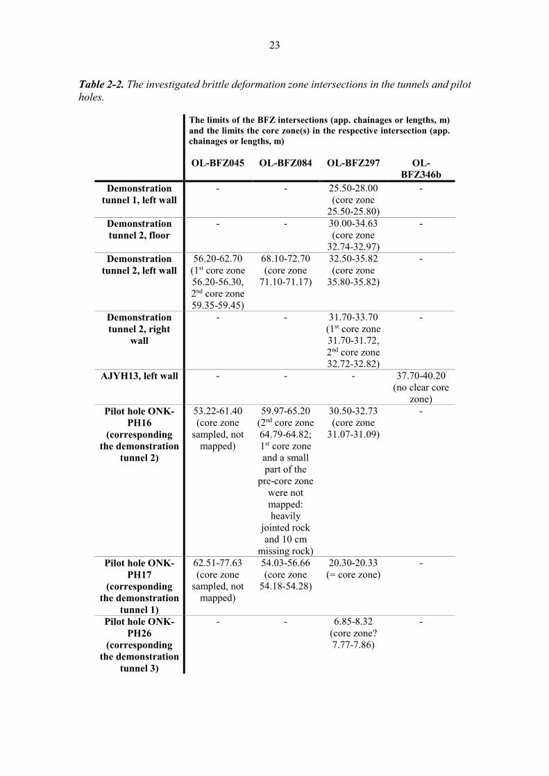
During the study, GSI values were directly mapped from several brittle deformation zone intersections of ONKALO. These intersections included one intersection in the demonstration tunnel 1, three intersections in the demonstration tunnel 2, one intersection in the vehicle connection tunnel AJYH13, and several intersections in the pilot holes (ONK-PH16, ONK-PH17, ONK-PH26) corresponding the demonstration tunnels 1-3. More detailed information about the locations of the mapped intersections is shown in Table 2-2 and in Chapters 2.1.1 - 2.1.4. The locations of the studied tunnel sections are illustrated in Figure 2-1.

These mapped GSI values are compared to the indirectly derived GSI values, which were calculated using three different conversion equations (see Chapter 3.4). These equations connect the GSI value to the Q´ value, to three of the Q´ parameters (RQD, Jr, Ja) or to two of the RMR89´ parameters (JCond89 and RQD). All parameters (RQD, Jn, Jr, Ja, JCond89) needed for these calculations were also mapped from the studied deformation zone intersections. In addition, other RMR89´ parameters were also mapped, including rock strength and spacing of the discontinuities.

For all mapped sections, RMR89´ values were obtained, instead of RMR89 values. In the case of the pilot hole sections, it was not possible to investigate the groundwater conditions. In the case of the tunnel sections, groundwater conditions were disturbed. The effect of the fracture orientations (tunnel drift) for the RMR89´ values of the tunnel sections was not investigated, because that was not important in the scope of this study.

The orientations (strike and dip) of the core zones of the brittle deformation zone intersections in the tunnel were also determined. Other fracture orientations in the deformation zone intersections were not systematically determined in this work.

Different parameters were determined separately for a pre-core zone (before the core zone), the core zone and the post-core zone (after the core zone). Sometimes were there two cores zones, which were mapped separately. In these cases, the zone between the cores was also mapped separately.

In the case of the pilot holes, some pre- or post-core zones were divided in several sections based on the rock type. All these were logged separately.

The total number of investigated sections was 45 of which the number of investigated core zones was 13. There were also three more core zones in the pilot holes, but they had been sampled and thus were not available for the investigations.

20

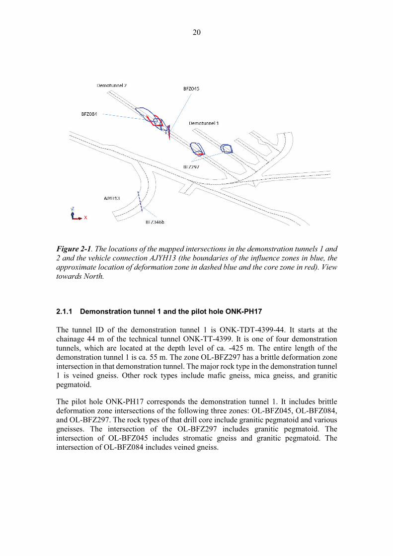
Figure 2-1. The locations of the mapped intersections in the demonstration tunnels 1 and 2 and the vehicle connection AJYH13 (the boundaries of the influence zones in blue, the approximate location of deformation zone in dashed blue and the core zone in red). View towards North.

2.1.1 Demonstration tunnel 1 and the pilot hole ONK-PH17

The tunnel ID of the demonstration tunnel 1 is ONK-TDT-4399-44. It starts at the chainage 44 m of the technical tunnel ONK-TT-4399. It is one of four demonstration tunnels, which are located at the depth level of ca. -425 m. The entire length of the demonstration tunnel 1 is ca. 55 m. The zone OL-BFZ297 has a brittle deformation zone intersection in that demonstration tunnel. The major rock type in the demonstration tunnel 1 is veined gneiss. Other rock types include mafic gneiss, mica gneiss, and granitic pegmatoid.

The pilot hole ONK-PH17 corresponds the demonstration tunnel 1. It includes brittle deformation zone intersections of the following three zones: OL-BFZ045, OL-BFZ084, and OL-BFZ297. The rock types of that drill core include granitic pegmatoid and various gneisses. The intersection of the OL-BFZ297 includes granitic pegmatoid. The intersection of OL-BFZ045 includes stromatic gneiss and granitic pegmatoid. The intersection of OL-BFZ084 includes veined gneiss.

21

2.1.2 Demonstration tunnel 2 and the pilot hole ONK-PH16

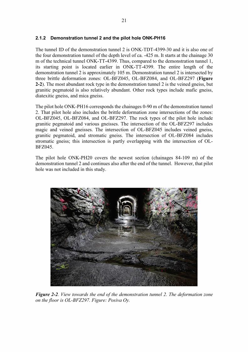
The tunnel ID of the demonstration tunnel 2 is ONK-TDT-4399-30 and it is also one of the four demonstration tunnel of the depth level of ca. -425 m. It starts at the chainage 30 m of the technical tunnel ONK-TT-4399. Thus, compared to the demonstration tunnel 1, its starting point is located earlier in ONK-TT-4399. The entire length of the demonstration tunnel 2 is approximately 105 m. Demonstration tunnel 2 is intersected by three brittle deformation zones: OL-BFZ045, OL-BFZ084, and OL-BFZ297 (Figure 2-2). The most abundant rock type in the demonstration tunnel 2 is the veined gneiss, but granitic pegmatoid is also relatively abundant. Other rock types include mafic gneiss, diatexitic gneiss, and mica gneiss.

The pilot hole ONK-PH16 corresponds the chainages 0-90 m of the demonstration tunnel 2. That pilot hole also includes the brittle deformation zone intersections of the zones: OL-BFZ045, OL-BFZ084, and OL-BFZ297. The rock types of the pilot hole include granitic pegmatoid and various gneisses. The intersection of the OL-BFZ297 includes magic and veined gneisses. The intersection of OL-BFZ045 includes veined gneiss, granitic pegmatoid, and stromatic gneiss. The intersection of OL-BFZ084 includes stromatic gneiss; this intersection is partly overlapping with the intersection of OL-BFZ045.

The pilot hole ONK-PH20 covers the newest section (chainages 84-109 m) of the demonstration tunnel 2 and continues also after the end of the tunnel. However, that pilot hole was not included in this study.

Figure 2-2. View towards the end of the demonstration tunnel 2. The deformation zone on the floor is OL-BFZ297. Figure: Posiva Oy.

22

2.1.3 The pilot hole ONK-PH26 (Demonstration tunnel 3)

One brittle deformation zone intersected by the pilot hole ONK-PH26 was also investigated within the study. This zone intersection represents an intersection of the zone OL-BFZ297. The rock type of that intersection is granitic pegmatoid; other rock types encountered in the core ONK-PH26 include diatexitic gneiss and veined gneiss.

The pilot hole ONK-PH26 corresponds the demonstration tunnel 3. There is also an intersection of OL-BFZ297 deformation zone in the demonstration tunnel 3, but it was not mapped during this study.

2.1.4 AJYH13

A brittle deformation zone intersection of the zone OL-BFZ346b in a vehicle access tunnel AJYH13 was also mapped in this study. The vehicle access tunnel AJYH13 is located near the demonstration tunnels (at ca. -425 m). The tunnel AJYH13 is a relatively short tunnel (“a dead end”) and its tunnel ID is ONK-TT-4366.

23

Table 2-2. The investigated brittle deformation zone intersections in the tunnels and pilot holes.

The limits of the BFZ intersections (app. chainages or lengths, m) and the limits the core zone(s) in the respective intersection (app. chainages or lengths, m)

OL-BFZ045 OL-BFZ084 OL-BFZ297 OL-

BFZ346b Demonstration

tunnel 1, left wall - - 25.50-28.00

(core zone 25.50-25.80)

-

Demonstration tunnel 2, floor

- - 30.00-34.63 (core zone

32.74-32.97)

-

Demonstration tunnel 2, left wall

56.20-62.70 (1st core zone 56.20-56.30, 2nd core zone 59.35-59.45)

68.10-72.70 (core zone

71.10-71.17)

32.50-35.82 (core zone

35.80-35.82)

-

Demonstration tunnel 2, right

wall

- - 31.70-33.70 (1st core zone 31.70-31.72, 2nd core zone 32.72-32.82)

-

AJYH13, left wall - - - 37.70-40.20 (no clear core

zone) Pilot hole ONK-

PH16 (corresponding

the demonstration tunnel 2)

53.22-61.40 (core zone

sampled, not mapped)

59.97-65.20 (2nd core zone 64.79-64.82; 1st core zone and a small part of the

pre-core zone were not mapped: heavily

jointed rock and 10 cm

missing rock)

30.50-32.73 (core zone

31.07-31.09)

-

Pilot hole ONK-PH17

(corresponding the demonstration

tunnel 1)

62.51-77.63 (core zone

sampled, not mapped)

54.03-56.66 (core zone

54.18-54.28)

20.30-20.33 (= core zone)

-

Pilot hole ONK-PH26

(corresponding the demonstration

tunnel 3)

- - 6.85-8.32 (core zone? 7.77-7.86)

-

24

2.2 JRC and JCS values

JRC (Joint Roughness Coefficient) and JCS (Joint wall Compressive Strength) values were also measured in this study to be able to investigate the applicability and the accuracy of the indirect ways to estimate these values from ONKALO mapping data (see Chapters 3.5.1 and 30). JRC and JCS values are used for characterizing individual discontinuities.

JRC and JCS values were estimated for six test fractures, outside of the brittle deformation zone intersections. The test fractures were located in the demonstration tunnel 1 (one fracture), the demonstration tunnel 2 (four fractures) and the shaft access tunnel ONK-KPE1-910 (one fracture). Finding suitable test fractures was not an easy task; for that reason, no more than six fractures were tested. The locations of the test fractures are listed in Table 2-3. JRC values were measured with a comb (a roughness profile tool) and the JCS values were derived based on the rebound values from Schmidt hammer measurements.

All necessary parameters for the indirect estimates of the JRC and JCS values were also mapped from these same test fractures. These parameters included Jr value of the fracture, the associated fracture (Jr) profile (see Appendix 1), the thickness of the mineral fill in the fracture and the rock type category (see Table 2-1) for the surrounding rock. JRC values can be estimated based on the Jr values and the associated fracture (Jr) profiles. JCS values can be calculated from the uniaxial compressive strength (UCS) of intact rock and an “alteration” value (a numerical value describing the alteration of the fracture). In this study, the applied intact rock UCS values were average intact rock UCS values for two rock type categories (see Chapter 3.6.1). The alteration value was defined based on the thickness of the mineral fill and the Jr profile, using the principles introduced by Salminen et al. (2018).

For informative and classification purposes, Ja values, fracture orientations (strike and dip) and approximate fracture lengths were also mapped.

Table 2-3. The test fractures measured for the JRC and JCS values. These fractures were also mapped for those properties, which were needed for the indirect ways to estimate JRC and JCS values.

Tunnel ID Location Demonstration tunnel 1 38.50 m (app. chainage) Demonstration tunnel 2 23.00 m (app. chainage) Demonstration tunnel 2 37.00 m (app. chainage) Demonstration tunnel 2 62.70 m (app. chainage) Demonstration tunnel 2 100.00 m (app. chainage) Shaft access tunnel ONK-KPE1-910 4.20 m (distance from the tunnel entrance)

25

3 THEORY AND FORMULATION BEHIND THE PARAMETERS

3.1 RQD (Rock Quality Designation) index

The Rock Quality Designation (RQD) index was defined by Deere (Deere 1963, Deere et al. 1967). It was developed to provide an estimate of rock mass quality from drill core logs. RQD is defined as the percentage of intact core pieces longer than 100 mm in the length of core being considered.

Five rock quality classes are defined according to the RQD value:

1. Very poor: 0-25 2. Poor: 25-50 3. Fair: 50-75 4. Good: 75-90 5. Excellent: 90-100

If no core is available but discontinuity traces are visible in surface exposures or exploration adits, the RQD values could be estimated with the equation of Palmström (2005). However, in this study, the RQD values of the tunnel sections were defined using artificial “scanlines” in the tunnel walls/floors.

3.2 The Rock Tunnelling Quality Index Q and the modified Tunnelling Quality Index Q´

The Rock Tunnelling Quality Index, Q, is defined by the following equation (e.g. Barton et al. 1974, Barton 2002, Grimstad & Barton 1993, NGI 2015):

𝑄𝑄 = 𝑅𝑅𝑅𝑅𝑅𝑅𝐽𝐽𝑛𝑛

× 𝐽𝐽𝑟𝑟𝐽𝐽𝑎𝑎

× 𝐽𝐽𝑤𝑤𝑆𝑆𝑅𝑅𝑆𝑆

Eq. 1

where

RQD = the Rock Quality Designation (see Chapter 3.1)

Jn = Joint set number

Jr = Joint roughness number

Ja = Joint alteration number

Jw = Joint water reduction number

SRF = Stress Reduction Factor

The Q value can range from 0.001 (exceptionally poor rock quality) to 1000 (exceptionally good rock quality).

26

The first quotient (RQD/Jn) of the Rock Tunnelling Quality index represents the structure of the rock mass (Barton et al. 1974). According to Barton et al. (1974), the first quotient is a crude measure of the block or particle size, with the two extreme values (100/0.5 and 10/20) differing by a factor of 400. Barton et al. (1974) write: “if the quotient is interpreted in units of centimetres, the extreme 'particle sizes' of 200 to 0.5 cm are seen to be crude but fairly realistic approximations. Probably the largest blocks will be several times this size and the smallest fragments less than half the size”. Theory of the RQD values is described in Chapter 3.1 and the Jn values are described in Appendix 1.

The second quotient (Jr/Ja) of the Rock Tunnelling Quality index is a measure of inter-block friction angle (Grimstad & Barton 1993). It represents the roughness and degree of alteration of the joint walls or filling materials (Barton et al. 1974). According to Barton et al. (1974), the following equation is a fair approximation of the actual shear strength:

𝑡𝑡𝑡𝑡𝑡𝑡−1(𝐽𝐽𝑟𝑟𝐽𝐽𝑎𝑎

) Eq. 2

The “friction angles” derived with Equation 2 are weighted in favour of rough unaltered fractures in direct contact. According to Barton et al. (1974): “it is to be expected that such surfaces will be close to peak strength, that they will tend to dilate strongly when sheared, and that they will therefore be especially favourable to tunnel stability”. These “friction angles” are similar to the total friction angles: combined cohesion and friction (Barton et al. 1974). Moreover, Equation 2 yields apparently dilatant (ϕ + i) friction angles for many joints and apparently contractile (ϕ – i) friction angles for many filled discontinuities (Barton 2002).

The strength of the fractures is significantly reduced, if they are even thin clay mineral coatings or fillings (Barton et al. 1974). However, rock wall contact after small shear displacements may be an important factor for preserving the excavation from ultimate failure. Where no rock wall contact exists, the conditions are extremely unfavourable to tunnel stability.

Further details about the Jr and Ja values are given in Appendix 1.

The third quotient (Jw/SRF) is a measure of the active stress (Grimstad & Barton 1993). It represents the relative effect of water, faulting, strength/stress ratio, squeezing or swelling (Barton 2002). This quotient consists of two stress parameters: Jw and SRF. According to Barton et al. (1974), “The parameter Jw is a measure of water pressure, which has an adverse effect on the shear strength of joints due to reduction in effective normal stress. Water may in addition cause softening and possible outwash in the case of clay filled joints. The parameter SRF is a measure of (1) loosening load in the case of excavation through shear zones and clay bearing rock, (2) rock stress in competent rock, (3) squeezing or swelling loads in plastic incompetent rock”.

Further details about the Jw and SRF values are given in Appendix 1. In this study, Jw and SRF values were not defined (see Chapter 4.1.2).

27

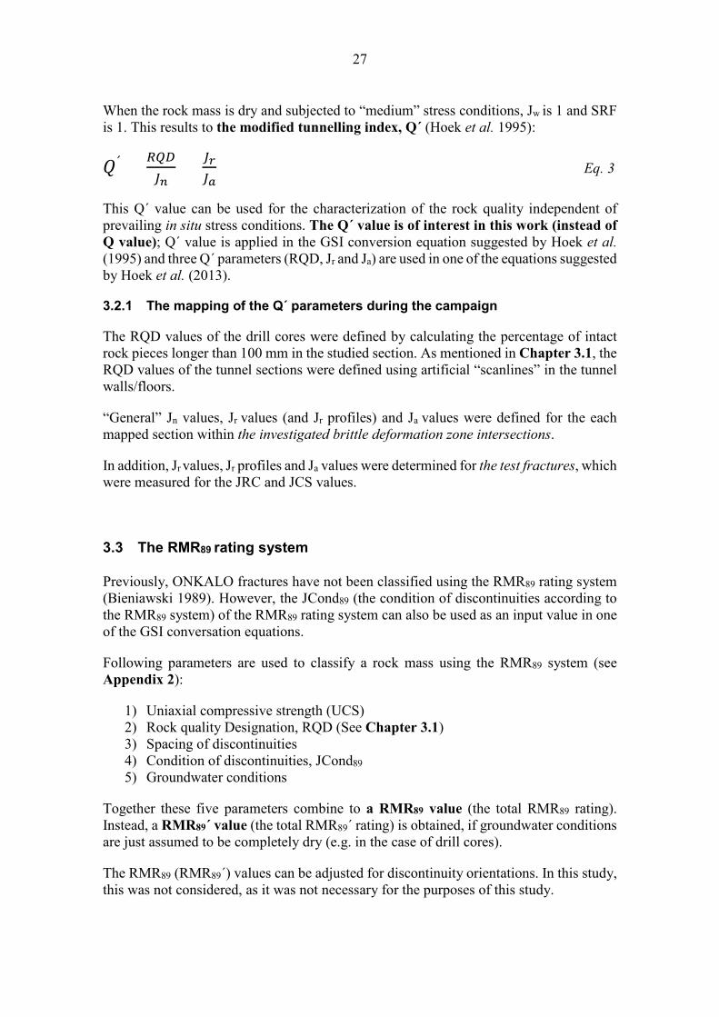
When the rock mass is dry and subjected to “medium” stress conditions, Jw is 1 and SRF is 1. This results to the modified tunnelling index, Q´ (Hoek et al. 1995):

𝑄𝑄´ = 𝑅𝑅𝑅𝑅𝑅𝑅𝐽𝐽𝑛𝑛

× 𝐽𝐽𝑟𝑟𝐽𝐽𝑎𝑎

Eq. 3

This Q´ value can be used for the characterization of the rock quality independent of prevailing in situ stress conditions. The Q´ value is of interest in this work (instead of Q value); Q´ value is applied in the GSI conversion equation suggested by Hoek et al. (1995) and three Q´ parameters (RQD, Jr and Ja) are used in one of the equations suggested by Hoek et al. (2013).

3.2.1 The mapping of the Q´ parameters during the campaign

The RQD values of the drill cores were defined by calculating the percentage of intact rock pieces longer than 100 mm in the studied section. As mentioned in Chapter 3.1, the RQD values of the tunnel sections were defined using artificial “scanlines” in the tunnel walls/floors.

“General” Jn values, Jr values (and Jr profiles) and Ja values were defined for the each mapped section within the investigated brittle deformation zone intersections.

In addition, Jr values, Jr profiles and Ja values were determined for the test fractures, which were measured for the JRC and JCS values.

3.3 The RMR89 rating system

Previously, ONKALO fractures have not been classified using the RMR89 rating system (Bieniawski 1989). However, the JCond89 (the condition of discontinuities according to the RMR89 system) of the RMR89 rating system can also be used as an input value in one of the GSI conversation equations.

Following parameters are used to classify a rock mass using the RMR89 system (see Appendix 2):

1) Uniaxial compressive strength (UCS) 2) Rock quality Designation, RQD (See Chapter 3.1) 3) Spacing of discontinuities 4) Condition of discontinuities, JCond89 5) Groundwater conditions

Together these five parameters combine to a RMR89 value (the total RMR89 rating). Instead, a RMR89´ value (the total RMR89´ rating) is obtained, if groundwater conditions are just assumed to be completely dry (e.g. in the case of drill cores).

The RMR89 (RMR89´) values can be adjusted for discontinuity orientations. In this study, this was not considered, as it was not necessary for the purposes of this study.

28

The uniaxial compressive strength (UCS) of the rock can be measured e.g. with a point load test or with a Schmidt hammer. In the field, rock strength can also be estimated using a knife and then evaluating the observations based on the ISRM index table (Brown 1981). In the mapping campaign, the rock strengths were also determined using a knife.

There are five classes for spacing of discontinuities in the RMR89 rating system. Condition of discontinuities, JCond89, is defined by multiple parameters (see Appendix 2). The total rating for JCond89 is the sum of the ratings of individual parameters.

In this study, a constant rating of 15 was used for the groundwater conditions (the parameter 5) in the case of all studied sections (see Chapter 4.1.3). So, we obtained RMR89´ values.

3.4 GSI conversion equations

GSI values are mapped by using a suitable GSI mapping chart (e.g. Hoek and Marinos, 2000); the only way to map GSI values is to use a mapping chart for the given rock mass conditions.

GSI values can also be calculated from other mapped parameters obtained by different mapping systems. In fact, there are multiple equations linking the GSI value to other mapping parameters. The classical conversion equation (Eq. 4) connecting the GSI value to the Q mapping system was presented by Hoek et al. (1995). New methodologies for the quantification of the GSI value have been presented in recent years (e.g. Cai et al. 2004, Hoek et al. 2013).

However, different conversation equations give different kind of results. Three conversation equations, applied in this study, are given below (Equations 4-6). The applicability of these equations for the conditions of the ONKALO facility was tested in this study. Hence, the mapped GSI values could provide more accurate information as they could be compared against indirectly derived GSI values. In addition, these mapped values can be used as “calibration values” when exploring the results of the different GSI conversation equations. When rock mass is mapped for the Q´ parameters, the RMR89´ parameters (JCond89 and RQD) and the GSI value, it could be possible to say which equation is applicable in ONKALO – if any.

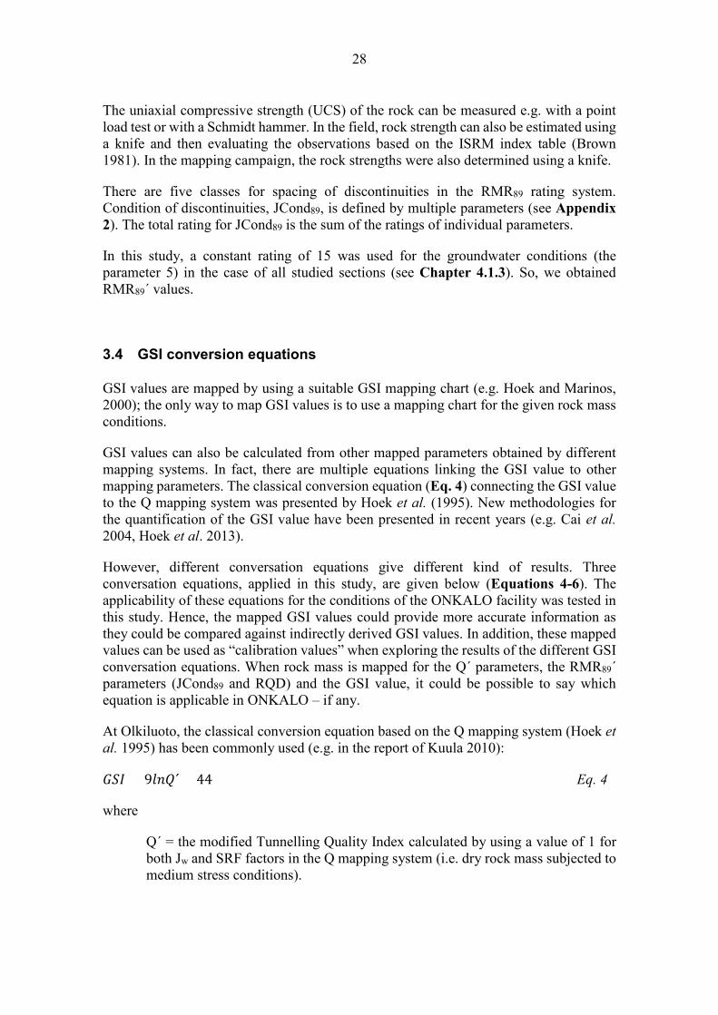
At Olkiluoto, the classical conversion equation based on the Q mapping system (Hoek et al. 1995) has been commonly used (e.g. in the report of Kuula 2010):

𝐺𝐺𝐺𝐺𝐺𝐺 = 9𝑙𝑙𝑡𝑡𝑄𝑄´ + 44 Eq. 4

where

Q´ = the modified Tunnelling Quality Index calculated by using a value of 1 for both Jw and SRF factors in the Q mapping system (i.e. dry rock mass subjected to medium stress conditions).

29

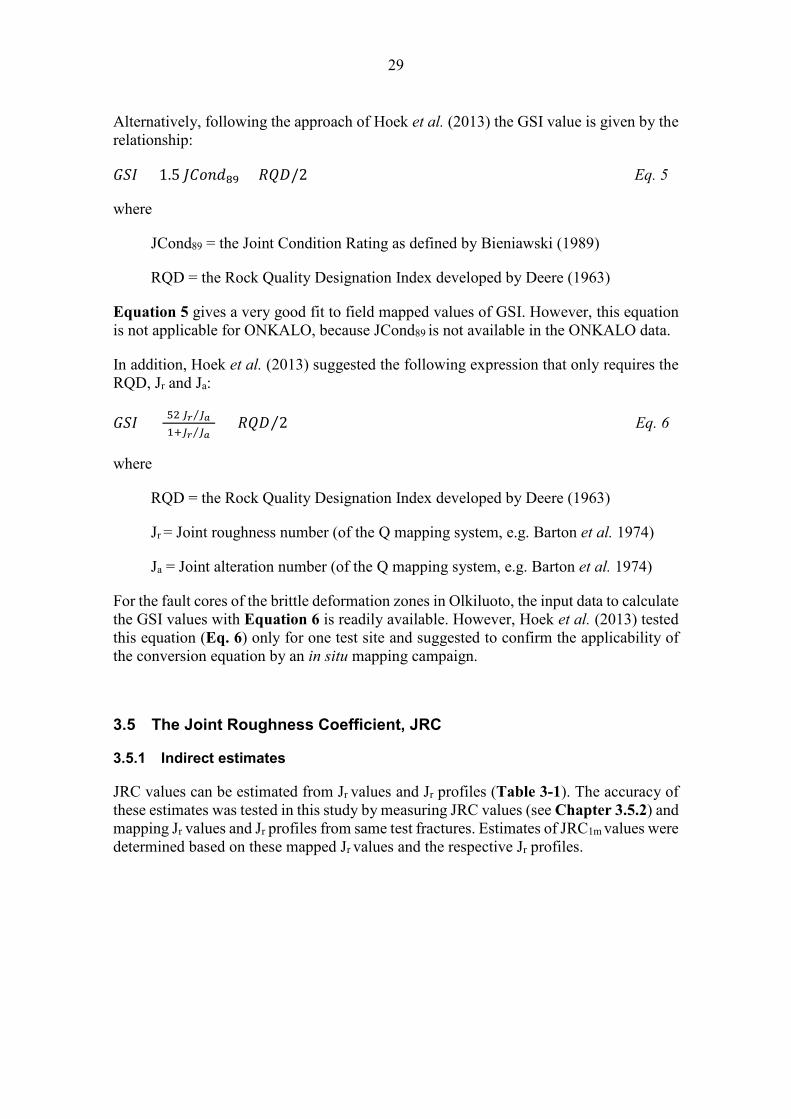
Alternatively, following the approach of Hoek et al. (2013) the GSI value is given by the relationship:

𝐺𝐺𝐺𝐺𝐺𝐺 = 1.5 𝐽𝐽𝐽𝐽𝐽𝐽𝑡𝑡𝐽𝐽89 + 𝑅𝑅𝑄𝑄𝑅𝑅/2 Eq. 5

where

JCond89 = the Joint Condition Rating as defined by Bieniawski (1989)

RQD = the Rock Quality Designation Index developed by Deere (1963)

Equation 5 gives a very good fit to field mapped values of GSI. However, this equation is not applicable for ONKALO, because JCond89 is not available in the ONKALO data.

In addition, Hoek et al. (2013) suggested the following expression that only requires the RQD, Jr and Ja:

𝐺𝐺𝐺𝐺𝐺𝐺 = 52 𝐽𝐽𝑟𝑟 𝐽𝐽𝑎𝑎⁄(1+𝐽𝐽𝑟𝑟 𝐽𝐽𝑎𝑎⁄ ) + 𝑅𝑅𝑄𝑄𝑅𝑅 2⁄ Eq. 6

where

RQD = the Rock Quality Designation Index developed by Deere (1963)

Jr = Joint roughness number (of the Q mapping system, e.g. Barton et al. 1974)

Ja = Joint alteration number (of the Q mapping system, e.g. Barton et al. 1974)

For the fault cores of the brittle deformation zones in Olkiluoto, the input data to calculate the GSI values with Equation 6 is readily available. However, Hoek et al. (2013) tested this equation (Eq. 6) only for one test site and suggested to confirm the applicability of the conversion equation by an in situ mapping campaign.

3.5 The Joint Roughness Coefficient, JRC

3.5.1 Indirect estimates

JRC values can be estimated from Jr values and Jr profiles (Table 3-1). The accuracy of these estimates was tested in this study by measuring JRC values (see Chapter 3.5.2) and mapping Jr values and Jr profiles from same test fractures. Estimates of JRC1m values were determined based on these mapped Jr values and the respective Jr profiles.

30

Table 3-1. Equivalence of the Jr value (the Q mapping system) and the JRC value. Table is obtained from the report of Salminen et al. (2018), after Barton (1987).

3.5.2 Measured JRC values

Before this mapping campaign, JRC measurements had not been performed in ONKALO. In this study, the JRC values were measured with a “comb” (a roughness profile tool; see Barton & Choubey 1977). For each measured surfaces, measurements were done separately in horizontal orientation and vertical orientation. Measurements were repeated 3 to 5 times for each orientation. After each measurement, the profile of the comb was compared to a classification scheme provided by Barton & Choubey (1977).

3.6 The Joint wall Compressive Strength, JCS

3.6.1 Indirect estimates

The JCS values can also be estimated from “the alteration value” of the fracture and the intact rock uniaxial compressive strength (UCS) of the host rock for the fracture, using the following equation (Barton 1973, Barton & Choubey 1977):

𝐽𝐽𝐽𝐽𝐺𝐺 = 𝑈𝑈𝑈𝑈𝑆𝑆𝑎𝑎𝑎𝑎𝑎𝑎𝑎𝑎𝑎𝑎𝑎𝑎𝑎𝑎𝑎𝑎𝑎𝑎𝑎𝑎

Eq. 7

31

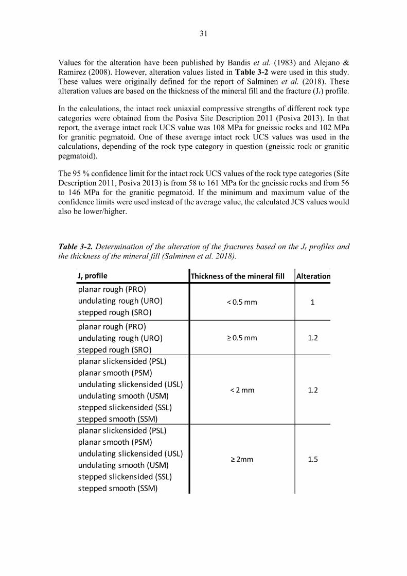
Values for the alteration have been published by Bandis et al. (1983) and Alejano & Ramirez (2008). However, alteration values listed in Table 3-2 were used in this study. These values were originally defined for the report of Salminen et al. (2018). These alteration values are based on the thickness of the mineral fill and the fracture (Jr) profile.

In the calculations, the intact rock uniaxial compressive strengths of different rock type categories were obtained from the Posiva Site Description 2011 (Posiva 2013). In that report, the average intact rock UCS value was 108 MPa for gneissic rocks and 102 MPa for granitic pegmatoid. One of these average intact rock UCS values was used in the calculations, depending of the rock type category in question (gneissic rock or granitic pegmatoid).

The 95 % confidence limit for the intact rock UCS values of the rock type categories (Site Description 2011, Posiva 2013) is from 58 to 161 MPa for the gneissic rocks and from 56 to 146 MPa for the granitic pegmatoid. If the minimum and maximum value of the confidence limits were used instead of the average value, the calculated JCS values would also be lower/higher.

Table 3-2. Determination of the alteration of the fractures based on the Jr profiles and the thickness of the mineral fill (Salminen et al. 2018).

Jr profile Thickness of the mineral fill Alteration

planar rough (PRO)undulating rough (URO)stepped rough (SRO)

< 0.5 mm 1

planar rough (PRO)undulating rough (URO)stepped rough (SRO)

≥ 0.5 mm 1.2

planar slickensided (PSL)planar smooth (PSM)undulating slickensided (USL)undulating smooth (USM)stepped slickensided (SSL)stepped smooth (SSM)

< 2 mm 1.2

planar slickensided (PSL)planar smooth (PSM)undulating slickensided (USL)undulating smooth (USM)stepped slickensided (SSL)stepped smooth (SSM)

≥ 2mm 1.5

32

3.6.2 JCS values from Schmidt hammer measurements

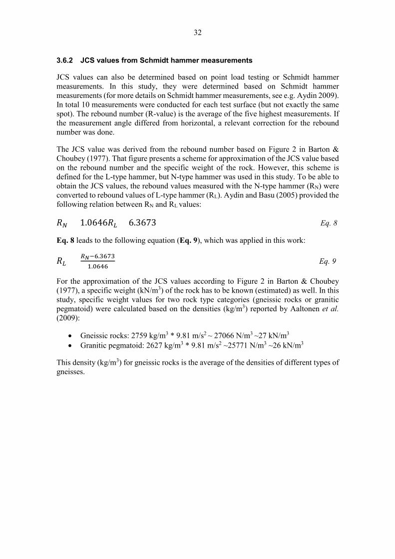
JCS values can also be determined based on point load testing or Schmidt hammer measurements. In this study, they were determined based on Schmidt hammer measurements (for more details on Schmidt hammer measurements, see e.g. Aydin 2009). In total 10 measurements were conducted for each test surface (but not exactly the same spot). The rebound number (R-value) is the average of the five highest measurements. If the measurement angle differed from horizontal, a relevant correction for the rebound number was done.

The JCS value was derived from the rebound number based on Figure 2 in Barton & Choubey (1977). That figure presents a scheme for approximation of the JCS value based on the rebound number and the specific weight of the rock. However, this scheme is defined for the L-type hammer, but N-type hammer was used in this study. To be able to obtain the JCS values, the rebound values measured with the N-type hammer (RN) were converted to rebound values of L-type hammer (RL). Aydin and Basu (2005) provided the following relation between RN and RL values:

𝑅𝑅𝑁𝑁 = 1.0646𝑅𝑅𝐿𝐿 + 6.3673 Eq. 8

Eq. 8 leads to the following equation (Eq. 9), which was applied in this work:

𝑅𝑅𝐿𝐿 = 𝑅𝑅𝑁𝑁−6.36731.0646

Eq. 9

For the approximation of the JCS values according to Figure 2 in Barton & Choubey (1977), a specific weight (kN/m3) of the rock has to be known (estimated) as well. In this study, specific weight values for two rock type categories (gneissic rocks or granitic pegmatoid) were calculated based on the densities (kg/m3) reported by Aaltonen et al. (2009):

• Gneissic rocks: 2759 kg/m3 * 9.81 m/s2 ~ 27066 N/m3 ~27 kN/m3 • Granitic pegmatoid: 2627 kg/m3 * 9.81 m/s2 ~25771 N/m3 ~26 kN/m3

This density (kg/m3) for gneissic rocks is the average of the densities of different types of gneisses.

33

4 RESULTS OF THE MAPPING CAMPAIGN

4.1 Brittle deformation zone intersections

The total number of investigated sections was 45 of which the number of investigated core zones was 13. There were also three more core zones in the pilot holes, but they had been sampled and thus were not available for the investigations.

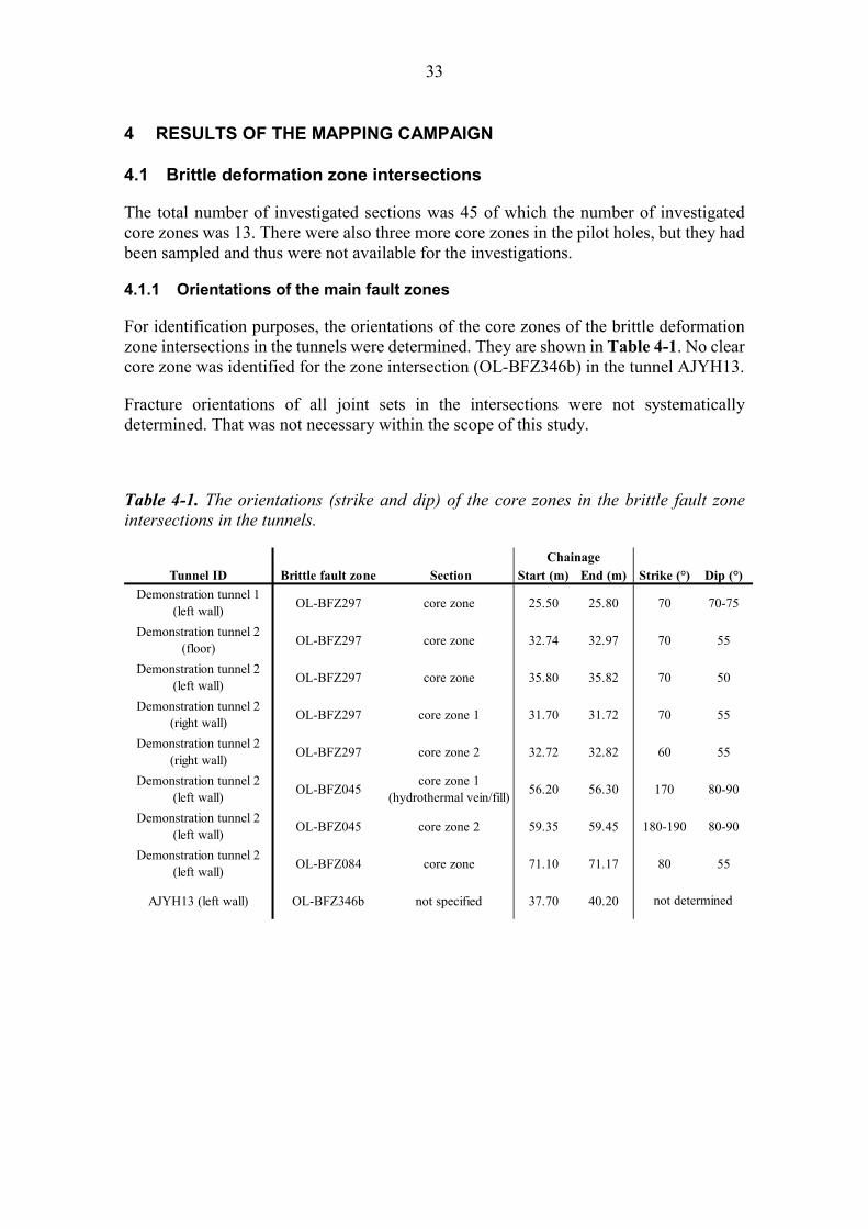
4.1.1 Orientations of the main fault zones

For identification purposes, the orientations of the core zones of the brittle deformation zone intersections in the tunnels were determined. They are shown in Table 4-1. No clear core zone was identified for the zone intersection (OL-BFZ346b) in the tunnel AJYH13.

Fracture orientations of all joint sets in the intersections were not systematically determined. That was not necessary within the scope of this study.

Table 4-1. The orientations (strike and dip) of the core zones in the brittle fault zone intersections in the tunnels.

Tunnel ID Brittle fault zone Section Start (m) End (m) Strike (°) Dip (°) Demonstration tunnel 1

(left wall) OL-BFZ297 core zone 25.50 25.80 70 70-75

Demonstration tunnel 2 (floor) OL-BFZ297 core zone 32.74 32.97 70 55

Demonstration tunnel 2 (left wall) OL-BFZ297 core zone 35.80 35.82 70 50

Demonstration tunnel 2 (right wall) OL-BFZ297 core zone 1 31.70 31.72 70 55

Demonstration tunnel 2 (right wall) OL-BFZ297 core zone 2 32.72 32.82 60 55

Demonstration tunnel 2 (left wall) OL-BFZ045

core zone 1 (hydrothermal vein/fill) 56.20 56.30 170 80-90

Demonstration tunnel 2 (left wall) OL-BFZ045 core zone 2 59.35 59.45 180-190 80-90

Demonstration tunnel 2 (left wall) OL-BFZ084 core zone 71.10 71.17 80 55

AJYH13 (left wall) OL-BFZ346b not specified 37.70 40.20 not determined

Chainage

34

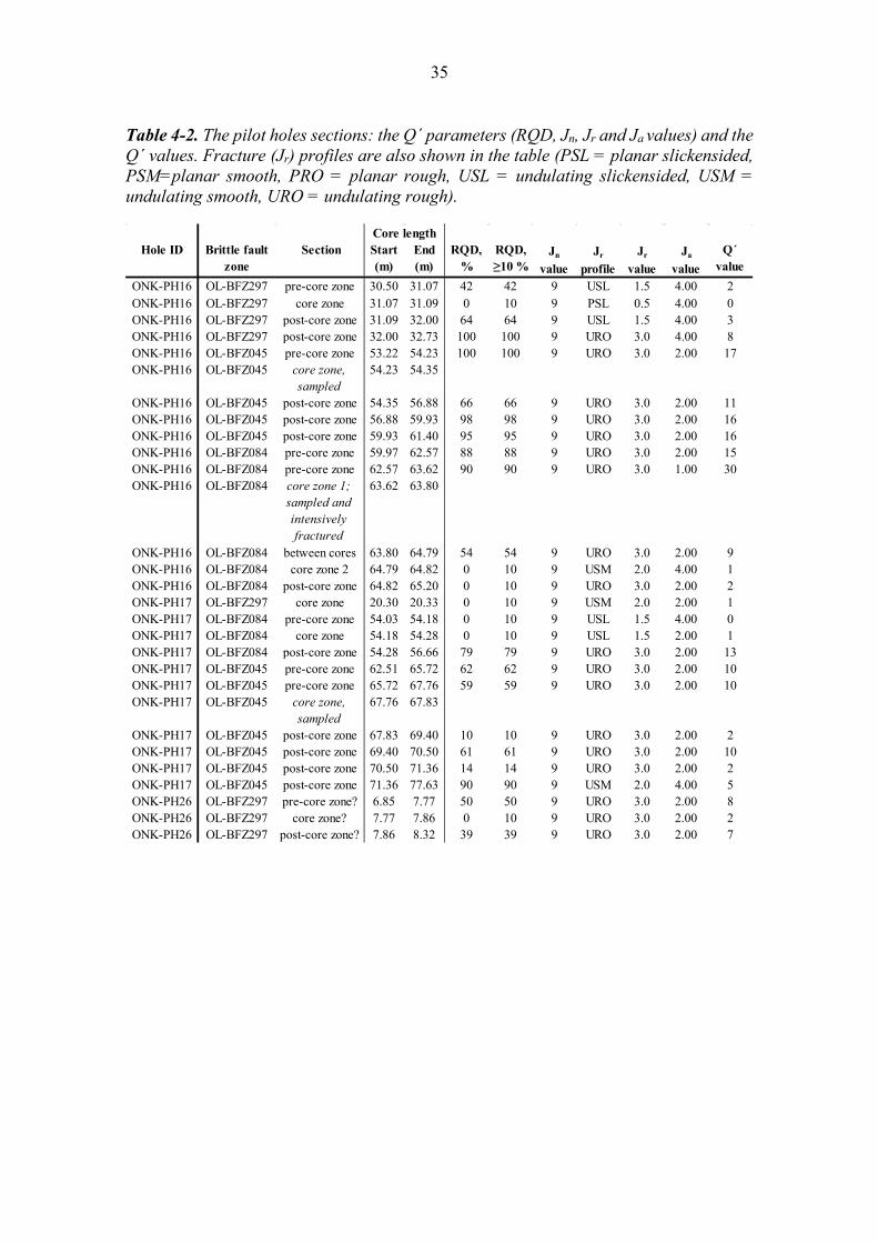
4.1.2 Q´ parameters

RQD, Jn, Jr and Ja values were determined for the studied sections within the brittle deformation zone intersections. These values are shown in Table 4-2 and Table 4-3.

For all mapped sections, Q´ values were obtained, instead of Q values. It is not even possible to determine SRF and Jw values for drill core sections. The SRF values were not either determined for all tunnel sections, as they were not necessary for the scope of this work. It would have not been possible to provide reliable estimates of Jw values for tunnel sections, as the groundwater conditions are disturbed. However, at the time of the mapping campaign, most the studied tunnel sections were dry. The fracture surfaces were damp in the core zone of the zone OL-BFZ084 in the demonstration tunnel 2, but it was uncertain where that water originated.

The logged RQD values vary from 0 to 100 %, but most of the RQD values of 0 % were obtained from the highly fractured core zones. The RQD values of the pre- and post-core zones, and the zones between cores, are commonly between 50 and 100 %. However, it is difficult to obtain reliable RQD values over a narrow rock section, especially in the case of 0-10 cm thick intersections.

A Jn value of 9 was applied for the studied pilot sections, as it was assumed that at least one joint set is not visible in drill cores. The logged Jn values of the tunnel sections are highly variable, from 1 to 12.

The mapped Jr values are commonly 2-3, but values of 0.5, 1.5 and 4 were also mapped in rare cases. The Jr value of 2 indicate smooth, undulating surface and the value of 3 indicate rough (irregular), undulating surface.

A majority of the mapped sections have a Ja value of 2, but values of 1 and 4 were also mapped. Thus, most of the mapped sections commonly have slightly altered joint walls.

35

Table 4-2. The pilot holes sections: the Q´ parameters (RQD, Jn, Jr and Ja values) and the Q´ values. Fracture (Jr) profiles are also shown in the table (PSL = planar slickensided, PSM=planar smooth, PRO = planar rough, USL = undulating slickensided, USM = undulating smooth, URO = undulating rough).

Hole ID Brittle fault zone

Section Start (m)

End (m)

RQD, %

RQD, ≥10 %

Jn

valueJr

profileJr

valueJa

valueQ´

valueONK-PH16 OL-BFZ297 pre-core zone 30.50 31.07 42 42 9 USL 1.5 4.00 2ONK-PH16 OL-BFZ297 core zone 31.07 31.09 0 10 9 PSL 0.5 4.00 0ONK-PH16 OL-BFZ297 post-core zone 31.09 32.00 64 64 9 USL 1.5 4.00 3ONK-PH16 OL-BFZ297 post-core zone 32.00 32.73 100 100 9 URO 3.0 4.00 8ONK-PH16 OL-BFZ045 pre-core zone 53.22 54.23 100 100 9 URO 3.0 2.00 17ONK-PH16 OL-BFZ045 core zone,

sampled54.23 54.35

ONK-PH16 OL-BFZ045 post-core zone 54.35 56.88 66 66 9 URO 3.0 2.00 11ONK-PH16 OL-BFZ045 post-core zone 56.88 59.93 98 98 9 URO 3.0 2.00 16ONK-PH16 OL-BFZ045 post-core zone 59.93 61.40 95 95 9 URO 3.0 2.00 16ONK-PH16 OL-BFZ084 pre-core zone 59.97 62.57 88 88 9 URO 3.0 2.00 15ONK-PH16 OL-BFZ084 pre-core zone 62.57 63.62 90 90 9 URO 3.0 1.00 30ONK-PH16 OL-BFZ084 core zone 1;

sampled and intensively fractured

63.62 63.80

ONK-PH16 OL-BFZ084 between cores 63.80 64.79 54 54 9 URO 3.0 2.00 9ONK-PH16 OL-BFZ084 core zone 2 64.79 64.82 0 10 9 USM 2.0 4.00 1ONK-PH16 OL-BFZ084 post-core zone 64.82 65.20 0 10 9 URO 3.0 2.00 2ONK-PH17 OL-BFZ297 core zone 20.30 20.33 0 10 9 USM 2.0 2.00 1ONK-PH17 OL-BFZ084 pre-core zone 54.03 54.18 0 10 9 USL 1.5 4.00 0ONK-PH17 OL-BFZ084 core zone 54.18 54.28 0 10 9 USL 1.5 2.00 1ONK-PH17 OL-BFZ084 post-core zone 54.28 56.66 79 79 9 URO 3.0 2.00 13ONK-PH17 OL-BFZ045 pre-core zone 62.51 65.72 62 62 9 URO 3.0 2.00 10ONK-PH17 OL-BFZ045 pre-core zone 65.72 67.76 59 59 9 URO 3.0 2.00 10ONK-PH17 OL-BFZ045 core zone,

sampled67.76 67.83

ONK-PH17 OL-BFZ045 post-core zone 67.83 69.40 10 10 9 URO 3.0 2.00 2ONK-PH17 OL-BFZ045 post-core zone 69.40 70.50 61 61 9 URO 3.0 2.00 10ONK-PH17 OL-BFZ045 post-core zone 70.50 71.36 14 14 9 URO 3.0 2.00 2ONK-PH17 OL-BFZ045 post-core zone 71.36 77.63 90 90 9 USM 2.0 4.00 5ONK-PH26 OL-BFZ297 pre-core zone? 6.85 7.77 50 50 9 URO 3.0 2.00 8ONK-PH26 OL-BFZ297 core zone? 7.77 7.86 0 10 9 URO 3.0 2.00 2ONK-PH26 OL-BFZ297 post-core zone? 7.86 8.32 39 39 9 URO 3.0 2.00 7

Core length

36

Table 4-3. The tunnel sections: the Q´ parameters (RQD, Jn, Jr and Ja values) and the Q´ values. Fracture (Jr) profiles are also show in the table (PSL = planar slickensided, PSM=planar smooth, PRO = planar rough, USL = undulating slickensided, USM = undulating smooth, URO = undulating rough, discont. = discontinuous).

Tunnel ID Brittle fault zone

Section Start (m)

End (m)

RQD, %

RQD, ≥10 %

Jn

valueJr

profileJr

valueJa

valueQ´

value

Demonstration tunnel 1 (left wall) OL-BFZ297 core zone 25.50 25.80 0 10 2 USM 2.0 4.00 3

Demonstration tunnel 1 (left wall) OL-BFZ297 post-core zone 25.80 28.00 78 78 6 USM 2.0 2.00 13

Demonstration tunnel 2 (floor) OL-BFZ297 pre-core zone 30.00 32.74 76 76 6 URO 3.0 2.00 19

Demonstration tunnel 2 (floor) OL-BFZ297 core zone 32.74 32.97 100 100 3 URO 3.0 2.00 50

Demonstration tunnel 2 (floor) OL-BFZ297 post-core zone 32.97 34.63 72 72 4 URO 3.0 2.00 27

Demonstration tunnel 2 (left wall) OL-BFZ297 pre-core zone 32.50 35.80 97 97 2 URO 3.0 1.00 145

Demonstration tunnel 2 (left wall) OL-BFZ297 core zone 35.80 35.82 0 10 2 USM 2.0 4.00 3

Demonstration tunnel 2 (right

wall)OL-BFZ297 core zone 1 31.70 31.72 0 10 2 USM 2.0 2.00 5

Demonstration tunnel 2 (right

wall)OL-BFZ297 between cores 31.72 32.72 100 100 1 discont. 4.0 1.00 400

Demonstration tunnel 2 (right

wall)OL-BFZ297 core zone 2 32.72 32.82 0 10 2 URO 3.0 4.00 4

Demonstration tunnel 2 (right

wall)OL-BFZ297 post-core zone 32.82 33.70 60 60 6 URO 3.0 2.00 15

Demonstration tunnel 2 (left wall) OL-BFZ045

core zone 1 (hydrothermal

vein/fill)56.20 56.30 100 100 1 URO 3.0 4.00 75

Demonstration tunnel 2 (left wall) OL-BFZ045 between cores 56.30 59.35 83 83 3 URO 3.0 2.00 42

Demonstration tunnel 2 (left wall) OL-BFZ045 core zone 2 59.35 59.45 0 10 2 USM 2.0 4.00 3

Demonstration tunnel 2 (left wall) OL-BFZ045 post-core zone 59.45 62.70 82 82 6 URO 3.0 2.00 21

Demonstration tunnel 2 (left wall) OL-BFZ084 pre-core zone 68.10 71.10 43 43 9 USM 2.0 4.00 2

Demonstration tunnel 2 (left wall) OL-BFZ084 core zone 71.10 71.17 0 10 2 USM 2.0 4.00 3

Demonstration tunnel 2 (left wall) OL-BFZ084 post-core zone 71.17 72.70 38 38 6 URO 3.0 2.00 9

AJYH13 (left wall) OL-BFZ346b not specified 37.70 40.20 86 86 12 URO 3.0 4.00 5

Chainage

37

4.1.3 RMR89´ ratings

The determined RMR89´ratings of the studied sections are given in Table 4-4 (the pilot hole sections) and Table 4-5 (the tunnel sections). In the case of the pilot holes, it was not possible to determine the groundwater conditions. The groundwater conditions in the tunnels were disturbed. So, a constant rating of 15 was applied for groundwater conditions in all cases.

In the case of the tunnel sections, the effect of fracture orientations (tunnel drift) on the RMR89´ ratings was not studied, because that was not necessary in the scope of this work. The effect of fracture orientations needs to be considered only when classifying the rock mass quality in order to get the right reinforcements etc.

As already mentioned in the case of the Q´ parameters (Chapter 4.1.2), most of the studied tunnel sections were dry at the time of the mapping campaign. The fracture surfaces were damp in the core zone of the zone OL-BFZ084 in the demonstration tunnel 2, but it was not sure where the water originated.

The variability of the RQD values was already presented in Chapter 4.1.2.

Rock strength ratings (estimated with a knife) vary from 2 to 15. Ratings of 7 and 12 are most commonly encountered in the mapping results. The rating of 7 corresponds to UCS values of 50-100 MPa and the rating of 12 corresponds to UCS values of 100-250 MPa. These estimates of the UCS values are of same magnitude as the UCS values of the intact rock of ONKALO (e.g. Posiva 2013). When compared to the laboratory testing statistics (Posiva 2013), the UCS values (5-50 MPa) corresponding the ratings 2-4 are probably too low and the UCS value (>250 MPa) corresponding the rating of 15 is likely too high.

The ratings for the spacing of discontinuities vary from 5 to 15. The rating of 5 means spacing <60 mm and the rating of 15 means spacing between 0.6 and 2 m.

The JCond89 values vary from 0 to 30, but in most cases JCond89 value is between 10 and 25.

38

Table 4-4. The RMR89´ ratings of the pilot hole sections: rock strength, RQD, spacing of discontinuities, condition of the discontinuities (JCond89) and the total RMR89´ rating.

Hole ID Brittle fault zone Section Start

(m)End (m)

1. Rock strength,

rating

2. RQD, rating

3. Spacing of discontinuities,

rating

4. Condition of the

discontinuities, rating (JCond89)

Total RMR89´ rating 1)

ONK-PH16 OL-BFZ297 pre-core zone 30.50 31.07 12 8 8 10 53ONK-PH16 OL-BFZ297 core zone 31.07 31.09 12 3 5 10 45ONK-PH16 OL-BFZ297 post-core zone 31.09 32.00 12 13 8 10 58ONK-PH16 OL-BFZ297 post-core zone 32.00 32.73 12 20 10 10 67ONK-PH16 OL-BFZ045 pre-core zone 53.22 54.23 7 20 10 25 77

ONK-PH16 OL-BFZ045 core zone, sampled 54.23 54.35 - - - - -

ONK-PH16 OL-BFZ045 post-core zone 54.35 56.88 7 13 8 25 68ONK-PH16 OL-BFZ045 post-core zone 56.88 59.93 12 20 10 25 82ONK-PH16 OL-BFZ045 post-core zone 59.93 61.40 7 20 8 23 73ONK-PH16 OL-BFZ084 pre-core zone 59.97 62.57 7 17 8 25 72ONK-PH16 OL-BFZ084 pre-core zone 62.57 63.62 12 20 10 25 82

ONK-PH16 OL-BFZ084

core zone 1; sampled and intensively fractured

63.62 63.80 - - - - -

ONK-PH16 OL-BFZ084 between cores 63.80 64.79 7 13 8 20 63ONK-PH16 OL-BFZ084 core zone 2 64.79 64.82 7 3 5 10 40ONK-PH16 OL-BFZ084 post-core zone 64.82 65.20 7 3 5 10 40ONK-PH17 OL-BFZ297 core zone 20.30 20.33 7 3 5 10 40ONK-PH17 OL-BFZ084 pre-core zone 54.03 54.18 12 3 5 15 50ONK-PH17 OL-BFZ084 core zone 54.18 54.28 7 3 5 10 40ONK-PH17 OL-BFZ084 post-core zone 54.28 56.66 12 17 8 23 75ONK-PH17 OL-BFZ045 pre-core zone 62.51 65.72 7 13 8 17 60ONK-PH17 OL-BFZ045 pre-core zone 65.72 67.76 12 13 8 20 68

ONK-PH17 OL-BFZ045 core zone, sampled 67.76 67.83 - - - - -

ONK-PH17 OL-BFZ045 post-core zone 67.83 69.40 12 3 8 23 61ONK-PH17 OL-BFZ045 post-core zone 69.40 70.50 12 13 8 23 71ONK-PH17 OL-BFZ045 post-core zone 70.50 71.36 12 3 5 23 58ONK-PH17 OL-BFZ045 post-core zone 71.36 77.63 12 20 8 15 70ONK-PH26 OL-BFZ297 pre-core zone? 6.85 7.77 15 8 8 27 73ONK-PH26 OL-BFZ297 core zone? 7.77 7.86 15 3 5 23 61ONK-PH26 OL-BFZ297 post-core zone ? 7.86 8.32 12 8 8 23 66

RMR89 ratings

1) A constant rating of 15 has been applied for the ground water conditions.

Core length

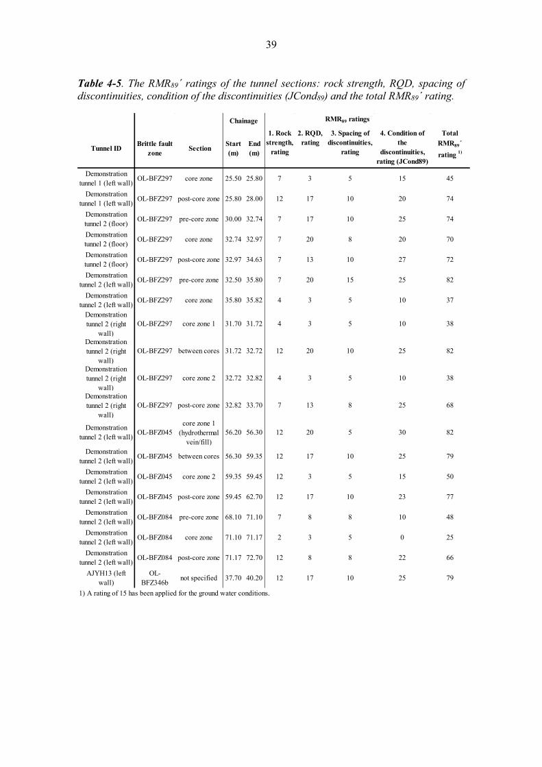
39

Table 4-5. The RMR89´ ratings of the tunnel sections: rock strength, RQD, spacing of discontinuities, condition of the discontinuities (JCond89) and the total RMR89´ rating.

Tunnel ID Brittle fault zone Section Start

(m)End (m)

1. Rock strength,

rating

2. RQD, rating

3. Spacing of discontinuities,

rating

4. Condition of the

discontinuities, rating (JCond89)

Total RMR89´ rating 1)

Demonstration tunnel 1 (left wall) OL-BFZ297 core zone 25.50 25.80 7 3 5 15 45

Demonstration tunnel 1 (left wall) OL-BFZ297 post-core zone 25.80 28.00 12 17 10 20 74

Demonstration tunnel 2 (floor) OL-BFZ297 pre-core zone 30.00 32.74 7 17 10 25 74

Demonstration tunnel 2 (floor) OL-BFZ297 core zone 32.74 32.97 7 20 8 20 70

Demonstration tunnel 2 (floor) OL-BFZ297 post-core zone 32.97 34.63 7 13 10 27 72

Demonstration tunnel 2 (left wall) OL-BFZ297 pre-core zone 32.50 35.80 7 20 15 25 82

Demonstration tunnel 2 (left wall) OL-BFZ297 core zone 35.80 35.82 4 3 5 10 37

Demonstration tunnel 2 (right

wall)OL-BFZ297 core zone 1 31.70 31.72 4 3 5 10 38

Demonstration tunnel 2 (right

wall)OL-BFZ297 between cores 31.72 32.72 12 20 10 25 82

Demonstration tunnel 2 (right

wall)OL-BFZ297 core zone 2 32.72 32.82 4 3 5 10 38

Demonstration tunnel 2 (right

wall)OL-BFZ297 post-core zone 32.82 33.70 7 13 8 25 68

Demonstration tunnel 2 (left wall) OL-BFZ045

core zone 1 (hydrothermal

vein/fill)56.20 56.30 12 20 5 30 82

Demonstration tunnel 2 (left wall) OL-BFZ045 between cores 56.30 59.35 12 17 10 25 79

Demonstration tunnel 2 (left wall) OL-BFZ045 core zone 2 59.35 59.45 12 3 5 15 50

Demonstration tunnel 2 (left wall) OL-BFZ045 post-core zone 59.45 62.70 12 17 10 23 77

Demonstration tunnel 2 (left wall) OL-BFZ084 pre-core zone 68.10 71.10 7 8 8 10 48

Demonstration tunnel 2 (left wall) OL-BFZ084 core zone 71.10 71.17 2 3 5 0 25

Demonstration tunnel 2 (left wall) OL-BFZ084 post-core zone 71.17 72.70 12 8 8 22 66

AJYH13 (left wall)

OL-BFZ346b not specified 37.70 40.20 12 17 10 25 79

1) A rating of 15 has been applied for the ground water conditions.

RMR89 ratingsChainage

40

4.1.4 GSI values

The mapped and calculated GSI values are given in Table 4-6 and Table 4-7.

It was not always so straightforward to determine the GSI values for the investigated pilot hole or tunnel sections. This was especially difficult in the case of the pilot holes and small deformation zone intersections (e.g. a couple of centimetres thick core zones). In fact, a range of the GSI values was given for the studied sections, instead of one single value. In the case of some tunnel sections, there were even two different options for these GSI ranges, depending on the observation scale.

The mapped GSI values of pilot hole sections are between 40 and 70. The mapped GSI values from the tunnel sections show variation from 10 to 85.

After the mapping of GSI ranges, the GSI values for same sections were calculated using three different equations:

• Equation 4, Hoek et al. 1995: “the conventional equation” (links the Q´ value to the GSI value).

• Equation 5, Hoek et al. 2013: links the JCond89 and RQD value to the GSI value. • Equation 6, Hoek et al. 2013: links the RQD, Jr and Jr values to the GSI value.

In this study, when using Eq. 6 (Hoek et al. 2013), the RQD values <10% were converted to values of 10 %.

For the tunnel intersections, Eq. 6 clearly most often gave GSI values closest to the mapped GSI values.

Also for the pilot hole intersections, Eq. 6 (Hoek et al. 2013) gave values close to the mapped ones, although the conventional equation (Eq. 4, Hoek et al. 1995) most often gave values closest to the mapped ones. For the logged core zones in the pilot holes, the conventional equation was better than Eq. 6.

Equation 5 (Hoek et al. 2013), linking the GSI values and the JCond89, less often gave the GSI values closest to the mapped ones – both in the case of the pilot holes and the tunnels.

For most of the studied sections (36 of 45 sections), a good match between the mapped and calculated GSI values was obtained with at least one of the three conversion equations. However, for three (3) of the sections, none of the equations provided equally good match; all these sections were pre- or post-core zones. For six (6) of the studied sections, GSI conversion equations did not provide good results at all; three of those sections were core zones.

41

Table 4-6. The pilot hole sections: the logged GSI values and the calculated GSI values.

Logged GSI

values

Hole ID Brittle fault zone Section Start

(m)End (m) Range

Hoek et al. 1995, from Q ́value (Eq. 4)

Hoek et al. 2013, from

JCond 89 and RQD (Eq. 5)

Hoek et al. 2013, from

RQD, J r and J a (Eq. 6) 1)

ONK-PH16 OL-BFZ297 pre-core zone 30.50 31.07 45-50 49 36 35ONK-PH16 OL-BFZ297 core zone 31.07 31.09 45-50 26 15 11ONK-PH16 OL-BFZ297 post-core zone 31.09 32.00 45-50 53 47 46ONK-PH16 OL-BFZ297 post-core zone 32.00 32.73 50-55 63 65 72ONK-PH16 OL-BFZ045 pre-core zone 53.22 54.23 55-65 69 88 81

ONK-PH16 OL-BFZ045 core zone, sampled 54.23 54.35 - - - -

ONK-PH16 OL-BFZ045 post-core zone 54.35 56.88 60-65 66 71 64ONK-PH16 OL-BFZ045 post-core zone 56.88 59.93 65-70 69 42 80ONK-PH16 OL-BFZ045 post-core zone 59.93 61.40 60-65 69 82 78ONK-PH16 OL-BFZ084 pre-core zone 59.97 62.57 60-65 68 82 75ONK-PH16 OL-BFZ084 pre-core zone 62.57 63.62 65-70 75 83 84

ONK-PH16 OL-BFZ084

core zone 1; sampled and intensively fractured

63.62 63.80 - - - -

ONK-PH16 OL-BFZ084 between cores 63.80 64.79 55-60 64 57 58ONK-PH16 OL-BFZ084 core zone 2 64.79 64.82 40-45 39 15 22ONK-PH16 OL-BFZ084 post-core zone 64.82 65.20 55-60 49 15 36ONK-PH17 OL-BFZ297 core zone 20.30 20.33 40-45 45 15 31ONK-PH17 OL-BFZ084 pre-core zone 54.03 54.18 65-70 36 23 19ONK-PH17 OL-BFZ084 core zone 54.18 54.28 40-45 42 15 27ONK-PH17 OL-BFZ084 post-core zone 54.28 56.66 65-70 67 74 71ONK-PH17 OL-BFZ045 pre-core zone 62.51 65.72 60-65 65 57 62ONK-PH17 OL-BFZ045 pre-core zone 65.72 67.76 55-60 65 60 61

ONK-PH17 OL-BFZ045 core zone, sampled 67.76 67.83 - - - -

ONK-PH17 OL-BFZ045 post-core zone 67.83 69.40 45-50 49 40 36ONK-PH17 OL-BFZ045 post-core zone 69.40 70.50 60-65 65 65 62ONK-PH17 OL-BFZ045 post-core zone 70.50 71.36 45-50 52 42 38ONK-PH17 OL-BFZ045 post-core zone 71.36 77.63 55-60 58 68 62ONK-PH26 OL-BFZ297 pre-core zone? 6.85 7.77 65-70 63 66 56ONK-PH26 OL-BFZ297 core zone? 7.77 7.86 50-55 49 35 36ONK-PH26 OL-BFZ297 post-core zone ? 7.86 8.32 50-60 61 54 51

1) RQD values <10 % were converted to values of 10 %.

Calculated GSI valuesCore length

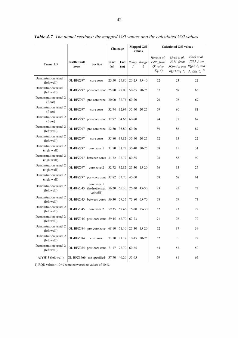
42

Table 4-7. The tunnel sections: the mapped GSI values and the calculated GSI values.

Tunnel ID Brittle fault zone Section Start

(m)End (m)

Range 1

Range 2

Hoek et al. 1995, from

Q ́value (Eq. 4)

Hoek et al. 2013, from

JCond 89 and RQD (Eq. 5)

Hoek et al. 2013, from

RQD, J r and J a (Eq. 6) 1)

Demonstration tunnel 1 (left wall) OL-BFZ297 core zone 25.50 25.80 20-25 35-40 52 23 22

Demonstration tunnel 1 (left wall) OL-BFZ297 post-core zone 25.80 28.00 50-55 70-75 67 69 65

Demonstration tunnel 2 (floor) OL-BFZ297 pre-core zone 30.00 32.74 60-70 70 76 69

Demonstration tunnel 2 (floor) OL-BFZ297 core zone 32.74 32.97 35-40 20-25 79 80 81

Demonstration tunnel 2 (floor) OL-BFZ297 post-core zone 32.97 34.63 60-70 74 77 67

Demonstration tunnel 2 (left wall) OL-BFZ297 pre-core zone 32.50 35.80 60-70 89 86 87

Demonstration tunnel 2 (left wall) OL-BFZ297 core zone 35.80 35.82 35-40 20-25 52 15 22

Demonstration tunnel 2 (right wall) OL-BFZ297 core zone 1 31.70 31.72 35-40 20-25 58 15 31

Demonstration tunnel 2 (right wall) OL-BFZ297 between cores 31.72 32.72 80-85 98 88 92

Demonstration tunnel 2 (right wall) OL-BFZ297 core zone 2 32.72 32.82 25-30 15-20 56 15 27

Demonstration tunnel 2 (right wall) OL-BFZ297 post-core zone 32.82 33.70 45-50 68 68 61

Demonstration tunnel 2 (left wall) OL-BFZ045

core zone 1 (hydrothermal

vein/fill)56.20 56.30 25-30 45-50 83 95 72

Demonstration tunnel 2 (left wall) OL-BFZ045 between cores 56.30 59.35 75-80 65-70 78 79 73

Demonstration tunnel 2 (left wall) OL-BFZ045 core zone 2 59.35 59.45 15-20 25-30 52 23 22

Demonstration tunnel 2 (left wall) OL-BFZ045 post-core zone 59.45 62.70 67-73 71 76 72

Demonstration tunnel 2 (left wall) OL-BFZ084 pre-core zone 68.10 71.10 25-30 15-20 52 37 39

Demonstration tunnel 2 (left wall) OL-BFZ084 core zone 71.10 71.17 10-15 20-25 52 0 22

Demonstration tunnel 2 (left wall) OL-BFZ084 post-core zone 71.17 72.70 60-65 64 52 50

AJYH13 (left wall) OL-BFZ346b not specified 37.70 40.20 55-65 59 81 65

Calculated GSI values

1) RQD values <10 % were converted to values of 10 %.

Mapped GSI values

Chainage

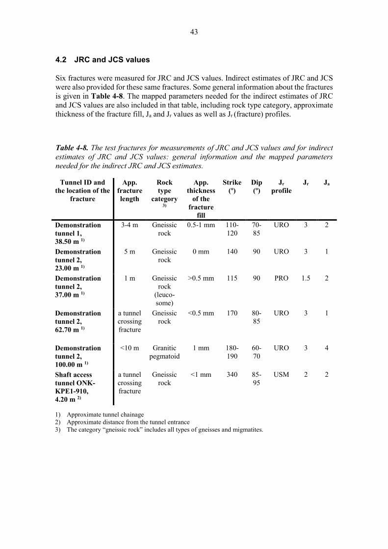
43

4.2 JRC and JCS values

Six fractures were measured for JRC and JCS values. Indirect estimates of JRC and JCS were also provided for these same fractures. Some general information about the fractures is given in Table 4-8. The mapped parameters needed for the indirect estimates of JRC and JCS values are also included in that table, including rock type category, approximate thickness of the fracture fill, Ja and Jr values as well as Jr (fracture) profiles.

Table 4-8. The test fractures for measurements of JRC and JCS values and for indirect estimates of JRC and JCS values: general information and the mapped parameters needed for the indirect JRC and JCS estimates.

Tunnel ID and the location of the

fracture

App. fracture length

Rock type

category 3)

App. thickness

of the fracture

fill

Strike (º)

Dip (º)

Jr

profile Jr Ja

Demonstration tunnel 1, 38.50 m 1)

3-4 m Gneissic rock

0.5-1 mm 110-120

70-85

URO 3 2

Demonstration tunnel 2, 23.00 m 1)

5 m Gneissic rock

0 mm 140 90 URO 3 1

Demonstration tunnel 2, 37.00 m 1)

1 m Gneissic rock

(leuco-some)

>0.5 mm 115 90 PRO 1.5 2

Demonstration tunnel 2, 62.70 m 1)

a tunnel crossing fracture

Gneissic rock

<0.5 mm 170 80-85

URO 3 1

Demonstration tunnel 2, 100.00 m 1)

<10 m Granitic pegmatoid

1 mm 180-190

60-70

URO 3 4

Shaft access tunnel ONK-KPE1-910, 4.20 m 2)

a tunnel crossing fracture

Gneissic rock

<1 mm 340 85-95

USM 2 2

1) Approximate tunnel chainage 2) Approximate distance from the tunnel entrance 3) The category “gneissic rock” includes all types of gneisses and migmatites.

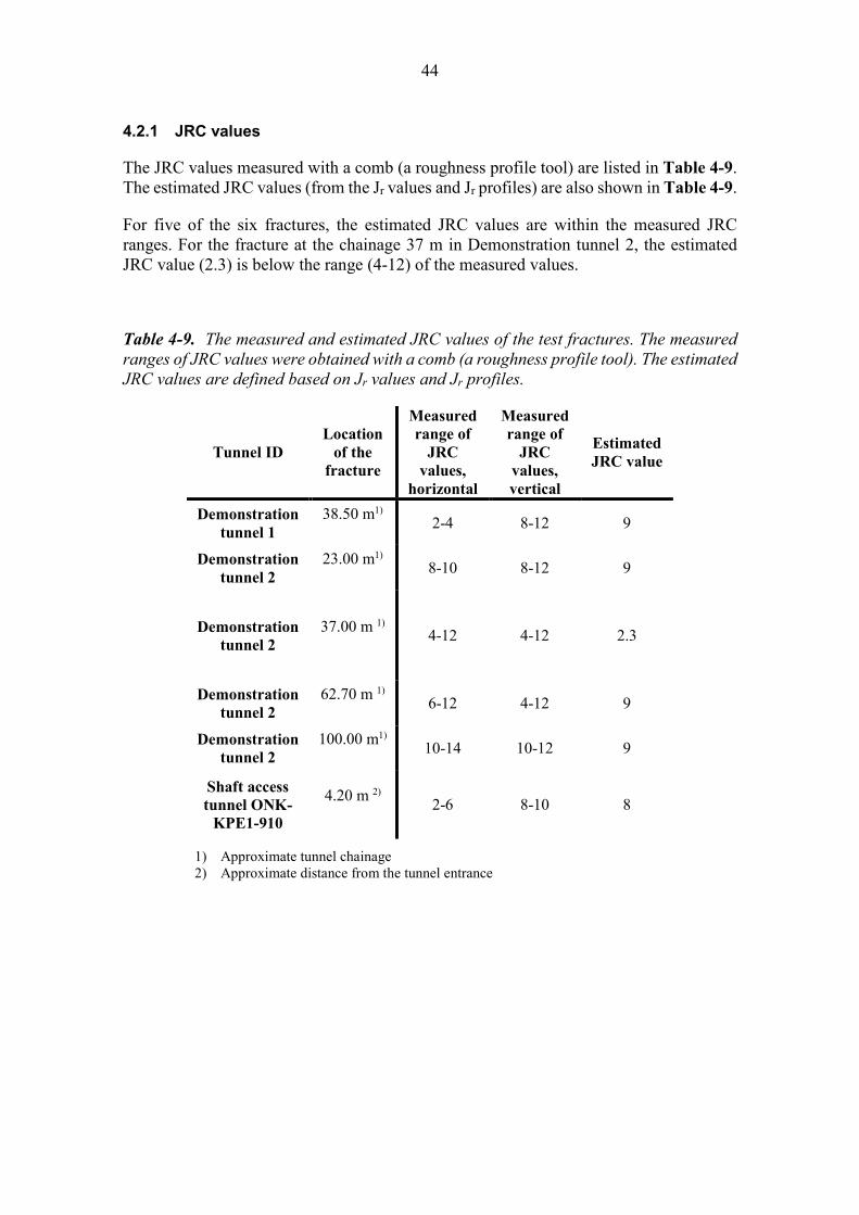
44

4.2.1 JRC values

The JRC values measured with a comb (a roughness profile tool) are listed in Table 4-9. The estimated JRC values (from the Jr values and Jr profiles) are also shown in Table 4-9.

For five of the six fractures, the estimated JRC values are within the measured JRC ranges. For the fracture at the chainage 37 m in Demonstration tunnel 2, the estimated JRC value (2.3) is below the range (4-12) of the measured values.

Table 4-9. The measured and estimated JRC values of the test fractures. The measured ranges of JRC values were obtained with a comb (a roughness profile tool). The estimated JRC values are defined based on Jr values and Jr profiles.

Tunnel ID Location

of the fracture

Measured range of

JRC values,

horizontal

Measured range of

JRC values, vertical

Estimated JRC value

Demonstration tunnel 1

38.50 m1) 2-4 8-12 9

Demonstration tunnel 2

23.00 m1) 8-10 8-12 9

Demonstration tunnel 2

37.00 m 1) 4-12 4-12 2.3

Demonstration tunnel 2

62.70 m 1) 6-12 4-12 9

Demonstration tunnel 2

100.00 m1) 10-14 10-12 9

Shaft access tunnel ONK-

KPE1-910

4.20 m 2) 2-6 8-10 8

1) Approximate tunnel chainage 2) Approximate distance from the tunnel entrance

45

4.2.2 JCS values

The rebound values from Schmidt hammer measurements and the corresponding JCS values are listed in Table 4-10. That table also includes the estimated JCS values, defined based on the thickness of the mineral fill, the fracture (Jr) profile and the average intact rock UCS value of the respective the rock type category (gneissic rock or granitic pegmatoid). The category “gneissic rocks” includes all types of gneisses and migmatites.

The measured JCS values are somewhat lower or higher than the estimated JCS values. However, these measured JCS values are not accurate values as their average dispersion is 20 to 100 MPa.

Table 4-10. The measured and estimated JCS values of the test fractures.

Tunnel ID Location

of the fracture

Rock type category

Measured JCS value

Estimated JCS value

4)

Schmidt hammer

rebound value (N-type

hammer)

Corresponding JCS value

(MPa) and its average

dispersion 3)

Demonstration tunnel 1 38.50 m1)

Gneissic rock 50 ~89 ± 20 108

Demonstration tunnel 2 23.00 m1)

Gneissic rock 51 ~92 ± 20 108

Demonstration tunnel 2 37.00 m 1)

Gneissic rock

(leucosome) 60 ~160 ± 60 90

Demonstration tunnel 2 62.70 m 1)

Gneissic rock 56 ~130 ± 80 108

Demonstration tunnel 2

100.00 m1)

Granitic pegmatoid 50 ~83 ± 20 85

Shaft access tunnel ONK-

KPE1-910 4.20 m 2)

Gneissic rock 61 ~170 ± 60 90-108

1) Approximate tunnel chainage 2) Approximate distance from the tunnel entrance 3) The rebound values obtained with the N-type hammer were converted to rebound values of

L-type hammer using Eq. 9 (derived from Eq. 8, after Aydin & Basu 2005). The JCS values were approximated from these calculated rebound values based on the Figure 2 in Barton & Choubey (1977). For more details, see Chapter 3.6.2.

4) Estimated JCS value is based on the average intact rock UCS value of the respective rock type category and the “alteration” value of the fracture (based on the thickness of the mineral fill and the fracture (Jr) profile)

46

47

5 DISCUSSION

5.1 Q´ values and RMR89´ values

Several rock sections within brittle deformation intersections were mapped for Q´ parameters and RMR89´ ratings. The total amount of studied rock sections was 45, including 26 sections in pilot holes and 19 tunnel sections.

The rock qualities were estimated based on the determined Q´ values and the RMR89´ values (the total RMR89´ ratings). However, Q´ and RMR89´ values can be used only for characterization of the rock mass, as the rock quality classifications are based on Q and RMR89 values (instead of the Q´ and RMR89´values). Thus, the rock qualities based on Q´ and RMR89´ values are just indicative estimates.

In the case of the pilot holes, the calculated Q´ values for the studied sections vary from 0 to 30. For 11/29 sections, the Q´ value is 0-4, indicating exceptionally poor to poor rock quality. Rest of the sections (15/29) are estimated to be of fair to good rock quality (Q´ value ≥5).

In the case of the tunnel sections, the calculated Q´ values vary from 2 to 400. For 6/19 sections, the Q´ value is between 2 and 4, indicating poor rock quality. For 8/19 sections, Q´ value is between 5 and 30, indicating fair to good rock quality. Rest (5/19) of the sections have a Q´ value of >30 and their estimated rock quality is very good to extremely good.

Based on the RMR89´ values, most of the studied pilot hole sections have fair to very good rock quality (RMR89´ values vary from 45 to 82). Three sections have a RMR89´ value of 40, which indicates poor rock quality.

Most of the tunnel sections have fair to good rock quality based on the RMR89´ values: RMR89´ values vary from 45 to 82. Four tunnel sections have RMR89´ values of 25-38, indicating poor rock quality.

When the rock qualities based on the Q´ and RMR89´ values are compared, they are commonly similar or in the next rock quality class (for example, the rock quality “fair” is “good” in the other classification system). In the case of some pilot sections, there is a difference of two rock quality classes (e.g. the rock quality “very poor” is “fair” in the other system) between the dedicated rock qualities. Tables showing the comparisons between the rock quality classes based on Q´ and RMR89´ values are included in Appendix 3.

5.2 GSI values

As mapping GSI values is more difficult for drill core sections than tunnel sections, it could be assumed that the mapped GSI values from the tunnel sections are more reliable. For the tunnel intersections, Equation 6 (Hoek et al. 2013, the equation linking the RQD, Jr and Ja values to the GSI values) most often gave the GSI values closest to the mapped

48

values. Based on that outcome, that equation (Eq. 6) could be recommended to be used in the case of ONKALO for further analyses.

Equation 6 also often gave values close to the mapped values in the case of pilot holes as well, although the conventional equation (Eq. 4, Hoek et al. 1995) was somewhat better for the pilot hole sections (especially for the core zones).

If the RQD values <10 % were used as they were (instead of converting them to values of 10 %) in Equation 6 (Hoek et al. 2013), the obtained GSI values were slightly lower and also less close to the mapped values. This difference was not significant, although it seems to be reasonable to convert these RQD values <10 % to values of 10 %. Some mapped RQD values <10 % have been afterwards noted to be typing errors or otherwise faulty values – thus, converting these values to a value of 10 % is justified.

The usage of the GSI values in the characterisation of the small rock sections, e.g. the core zones of the brittle deformation zones, is questionable. GSI mapping charts are not intended for the mapping of very small rock sections (perhaps only a few centimetres). In addition, GSI mapping of the drill cores is also challenging because of the “2D nature” of the drill core data – the true extents and continuations of the features (e.g. fractures) in the cores cannot be readily seen.

For six investigated sections, all calculated GSI values were far away from the mapped ones. Three of these six sections were core zones. Thus, the mapping or calculation of GSI values for small sections may indeed result in wrong outcomes. However, even for narrow core zones, some calculated values are close to the mapped ones.

5.3 JRC and JCS values

In the report of Salminen et al. (2018) (and its synthesis report provided by Salminen 2018), indirect JRC and JCS estimates are provided for fractures (outside of the brittle deformation zone intersections) in the area of the entire ONKALO facility. Those JRC and JCS estimates were further used in the calculations of stiffness parameters, instantaneous cohesion values, instantaneous friction angles, and peak dilation angles. So, this mapping campaign was needed to justify the usage of these indirect estimates in the report of Salminen et al. (2018).

5.3.1 JRC values

In most cases (5/6 fractures), the indirect estimates of the JRC values fit well in the measured ranges of JRC values. The usage of the indirect JRC estimates (from the Jr values and Jr profiles) seems to be acceptable – especially when taking in account the measured JRC values are not either accurate, single values. The mapping of JRC values provided ranges of JRC values, which were sometimes quite wide.

The outcome of the study would have been more reliable if the amount of tested fractured would have been greater. However, it was difficult to find suitable test fractures.

49

5.3.2 JCS values

The measured JCS values (based on the Schmidt hammer measurements) are somewhat lower or higher than the estimated JCS values (based on the average intact UCS value of the respective rock type category and the “alteration” value of the fracture surface). However, the measured JCS values are not very accurate values as their average dispersion is 20 to 100 MPa. In addition, the average intact rock UCS values were used in the calculations of the estimated JCS values. The estimated JCS values would have been different if the minimum or maximum values of the 95 % confidence limits for the intact rock UCS values had been used in the calculations instead of the average values. The resulting JCS values would have been up to 50 MPa lower if the minimum intact rock UCS values had been used and up to 53 MPa higher if the maximum intact rock UCS values had been applied. Thus, taken in account the inaccuracies of the both methods, the measured and estimated JCS values are not very far away from each other.

Anyhow, the highest ones of the measured JCS can be equal or even higher than the average intact rock UCS values for the respective rock type categories (see Chapter 3.6.1). The JCS value of an individual fracture surface cannot be higher than the (correct) UCS value of surrounding intact rock, although it can be close to that UCS value. This is the also the logics behind estimating of the JCS value of a certain fracture based on the intact rock UCS value of the surrounding rock matrix and the alteration value of that fracture. Thus, the fracture surfaces within the rock mass are inherently weaker than the intact rock matrix.

It must be also pointed out that the number of tested fractures was low (n = 6). In addition, the thickness of coating/fill in the tested fractures was small and the Schmidt hammer measurements were made on relatively fresh surfaces. It remains unsolved whether the results of this study are also applicable for fractures with thicker coatings /fills.

50

51

6 CONCLUSIONS

6.1 GSI values

GSI values were mapped from several pilot hole and tunnel sections within brittle deformation zone intersections. Simultaneously, other parameters were mapped from these same sections for the calculations of the GSI values using three different conversion equations. These parameters included RQD, Jn, Ja, Jr and JCond89 values. In addition, other RMR89´ parameters were also mapped. Orientations of the main fault zones in the tunnels were also determined. For the studied rock sections within the brittle deformation zone intersections, the rock qualities estimated based on the Q´ and the RMR89´ values were relatively similar.

GSI values were calculated based on other mapped parameters using three different conversion equations. The conventional equation (Eq. 4) of Hoek et al. (1995) links the Q´ value to the GSI value. One equation (Eq. 5) provided by Hoek et al. (2013) links the JCond89 and RQD values to the GSI value. Another equation (Eq. 6) of Hoek et al. (2013) links the RQD, Jr and Jr values to the GSI value.

In the case of the tunnel sections, the equation (Eq. 6) of Hoek et al. (2013) linking the RQD, Jr and Ja values to the GSI values, most often provided the best match between the calculated and mapped GSI values.

In the case of the pilot hole sections, the conventional equation (Eq. 4) of Hoek et al. (1995) most often provided the best fit between the mapped and calculated GSI values. However, Eq. 6 (Hoek et al. 2013) also provided generally good results. Moreover, GSI mapping of drill core intersections is not as reliable as the GSI mapping of the wider tunnel sections.

In this study, the RQD values <10 % were converted to values of 10 % when applying Eq. 6 of Hoek et al. (2013). Applying this principle, this equation gave the more precise GSI values compared to the mapped ones. However, even when using the RQD values as they were, this equation still usually provided GSI values close to the mapped ones.

In general, Equation 5 (Hoek et al. 2013) can be regarded less applicable for the conditions of ONKALO than the two other equations (Eq. 4 and Eq. 6).

For most of the studied sections (36 of 45 sections), a good match between the mapped and calculated GSI values was obtained with at least one of the three conversion equations. However, for three (3) of the sections none of the equations provided equally good match and for six (6) of the sections none of the GSI conversion equations provided good results at all.

So, for the conditions of ONKALO in general, Eq. 6 (Hoek et al. 2013) is recommended to be used when deriving GSI values from other mapped parameters. It is also advised to convert any RQD values <10 % to values of 10 % to obtain the best possible results with this equation.

52

6.2 JRC and JCS values

JRC and JCS values were measured for six test fractures, outside of the brittle deformation zone intersections. JRC and JCS values were also estimated for these same fractures based on other mapped parameters. So, the parameters needed for these indirect determinations were mapped from the fractures: Jr values, Jr profiles, thickness of the mineral fill, rock type category. Some more additional parameters were also determined (Ja values, fracture orientations, fracture trace lengths) from the fractures.

JRC values were measured with a “comb” (a roughness profile tool). A range of JRC values was obtained for each fracture. Some of these ranges were quite wide. The indirectly estimated JRC values were based on the Jr values and Jr profiles of the fractures. These estimated JRC values fitted within the measured JRC ranges in 5/6 study cases. Thus, the usage of the indirect JRC estimates seems to be acceptable – especially when taking account that the measured JRC values are not either accurate, single values. However, the results would have been more reliable if it had been possible to test more fractures.

The measured JCS values were derived based on the Schmidt hammer measurements. The estimated JCS values were based on the alteration value of the fracture and the intact rock UCS value for the respective rock type category. The measured JCS values turned out to be somewhat lower or higher than the indirectly estimated JCS values. However, there are inaccuracies in the determination of both types of JCS values. Taken in account these inaccuracies, the measured and estimated values are not far away from each other. So, it seems the methodology for indirectly estimating JCS values is applicable. However, only six fractures were tested and the thickness of coating/fill was small in all of these fractures.

53

7 REFERENCES

Aaltonen, I., Heikkinen, E., Paulamäki, S., Säävuori, H., Vuoriainen, S. & Öhman, I., 2009. Summary of Petrophysical Analysis of Olkiluoto Core Samples 1990-2008. Posiva Oy, Working Report 2009-11.

Aaltonen, I. (ed.), Engström, J., Front, K., Gehör, S., Kosunen, P., Kärki, A., Paananen, M., Paulamäki, S. & Mattila, J., 2016. Geology of Olkiluoto. Posiva Report 2016-16. Posiva Oy, Eurajoki.

Aaltonen, I. (ed.), Lahti, M., Engström, J., Mattila, J., Paananen, M., Paulamäki, S., Gehör, S., Kärki, A., Ahokas, T., Torvela, T. & Front, K., 2010. Geological Model of the Olkiluoto Site - version 2.0. Working Report 2010-70. Posiva Oy, Eurajoki. 580 p.

Alejano L. & Ramírez P., 2008. Mecánica de Rocas: Fundamentos e ingeniería de taludes. Ed Red DESIR. In Spanish.

Ask, D., 2011. Semi-integration analysis of overcoring stress data and review of rock stress data at the Olkiluoto site. Working Report 2011-16. Posiva Oy, Eurajoki.

Aydin, A., 2009. ISRM Suggested method for determination of the Schmidt hammer rebound hardness: Revised version. International Journal of Rock Mechanics & Mining Sciences 46, 627–634.

Aydin, A. & Basu, A., 2005. The Schmidt hammer in rock material characterization. Engineering Geology 81, 1-14.

Bandis, S.C., Lumsden, A.C. & Barton, N.R., 1983. Fundamentals of rock joint deformation. International Journal of Rock Mechanics and Mining Sciences & Geomechanics Abstracts 20, 249-268.

Barton, N., 1973. Review of a new shear-strength criterion for rock joints. Engineering Geology 7, 287-332.

Barton, N., 1987. Predicting the behaviour of underground openings in rock. In: “Manuel Rocha Memorial Lecture”. Lisbon. NGI, Oslo, Norway.

Barton, N., 2002. Some new Q-value correlations to assist in site characterisation and tunnel design. International Journal of Rock Mechanics and Mining Sciences 39, 185–216.

Barton, N. & Bandis, S., 1982. Effect of block size on the shear behaviour of jointed rock. Conference Proceedings “23rd U.S. Symposium on Rock Mechanics”, pp 739-760, Berkeley.

Barton, N. & Choubey, V., 1977. Thbandise shear strength of rock joints in theory and practice. Rock Mechanics 10, 1-54.

Barton, N., Lien, R. & Lunde, J., 1974. Engineering classification of rock masses for the design of tunnel support. Rock Mechanics 6, 198-236.

54

Bieniawski, Z.T., 1989. Engineering Rock Mass Classifications. A Complete Manual for Engineers and Geologists in Mining,Civil, and Petroleum Engineering. New York: Wiley Interscience.

Brown, E.T., 1981. Rock Characterization Testing and Monitoring. ISRM Suggested Methods.

Cai, M., Kaiser, P.K., Uno, H., Tasaka, Y. & Minami, M., 2004. Estimation of rock mass deformation modulus and strength of jointed hard rock masses using the GSI system. International Journal of Rock Mechanics & Mining Sciences 41, 3–19.

Chapman, N., Bath, A., Geier, J. & Stephansson, O., 2015. The disposal site and underground construction: Part I: The disposal site and the natural barrier : Part II: Preserving the favourable properties of the bedrock during construction. STUK Technical Report STUK-TR 17.

Deere, D.U., 1963. Technical description of rock cores for engineering purposes. Felsmechanik und Ingenieurgeologie (Rock Mechanics and Engineering Geology), 1, 16-22.

Deere, D.U., Hendron, A.J., Patton, F.D. & Cording, E.J., 1967. Design of surface and near surface construction in rock. Failure and breakage of rock: Proceedings of the 8th U.S. Symposium on Rock Mechanics (ed. C. Fairhurst), American Institute of Mining, Metallurgical & Petroleum Engineers, New York, pp. 237-302.Engström & Kemppainen 2008

Engström, J. & Kemppainen, K., 2008. Evaluation of the Geological and Geotechnical Mapping Procedures in use in the ONKALO Access Tunnel. Eurajoki, Finland: Posiva Oy. Working report 2008-77. Posiva Oy, Eurajoki.

Grimstad, E. & Barton, N., 1993. Updating of the Q-system for NMT. Proceedings of the International Symposium on Sprayed Concrete – Modern Use of Wet Mix Sprayed Concrete for Underground Support, Fagernes (eds. Kompen, Opsahl & Berg), Norwegian Concrete Association, Oslo.

Hakala, M., Hakala, V., Heine, J., Kemppainen, K., Savunen, J., Sireni, S., Siren, T., Ström, J., Valli, J., 2016. In Situ stress measurements in ONKALO with LVDT – Cell. Posiva 2016-20. Posiva Oy, Eurajoki, Finland.

Hakala, M., Siren, T., Kemppainen, K., Christiansson, R., Martin, D., 2014. In situ Stress Measurement with the New LVDT-Cell – Method Description and Verification. Posiva 2012-43. Posiva Oy, Eurajoki, Finland.

Hoek, E., Kaiser, P. K. & Bawden, W. F., 1995. Support of underground excavations in hard rocks. Rotterdam: A. A. Balkema.

Hoek, E., Carranza-Torres C. & Corkum, B., 2002. Hoek-Brown failure criterion. 2002 edition. Proceedings of the 5th North American Rock Mechanics Symposium and 17th Tunneling Association of Canada Conference: NARMS-TAC 2002, July 7-10, University of Toronto, pp. 267-271.

55

Hoek, E., Carter, T.G. & Diederichs, M.S., 2013. Quantification of the Geological Strength Index chart. Proceedings of the 47th US Rock Mechanics/Geomechanics Symposium, San Francisco, CA, USA, 23-26 June 2013. ARMA 13-672.

Hudson, J.A., Cosgrove, J. & Johansson, E., 2008. Estimating the mechanical properties of the brittle deformation zones at Olkiluoto. Working Report 2008–67. Posiva Oy, Eurajoki.

Korhonen, K-H., Gardemeister, R., Jääskeläinen, H., Niini, H. & Vähäsarja, P., 1974. Rakennusalan kallioluokitus. Valtion teknillinen tutkimuskeskus 12, Otaniemi, 78. (In Finnish.)

Kuula, H., 2010. Geometrical and Mechanical Properties of the Fractures and Brittle Deformation Zones based on ONKALO Tunnel Mapping, 0–2400 m Tunnel Chainages. Working Report 2010-64. Posiva Oy, Eurajoki.

Mattila, J., Aaltonen, I., Kemppainen, K. Wikström, L., Paananen, M., Paulamäki, S., Front, K. Gehör, S., Kärki, A. & Ahokas, T., 2008. Geological model of the Olkiluoto Site. Version 1.0. Working Report 2007-92. Posiva Oy, Eurajoki.

Mönkkönen, H., Rantanen, T. & Kuula, H., 2012. Geometrical and Mechanical Properties of the Fractures and Brittle Deformation Zones based on ONKALO Tunnel Mapping, 2400–4390 m Tunnel Chainages. Working Report 2010-64. Posiva Oy, Eurajoki.

NGI 2015. Using the Q-system. Handbook, NGI. Oslo, Norway.

Niinimäki, R., 2004. Core Drilling of Pilot Hole OL-PH1 at Olkiluoto in Eurajoki 2003-2004. Working Report 2005-06. Posiva Oy, Eurajoki.

Norokallio, J., 2015. Geological and Geotechnical Mapping Procedures in use in the ONKALO. Posiva 2015-01. Posiva Oy, Eurajoki.

Palmström, A., 2005. Measurements of and Correlations between Block Size and Rock Quality Designation (RQD). Tunnels and Underground Space Technology 20, 362-277.

Posiva 2013. Olkiluoto Site Description 2011. Posiva Report 2011-02. Posiva Oy, Eurajoki.

Salminen, P., 2018 (Expected in 2018). Rock Mechanics Parametrization of Fractures and Brittle Deformation Zones of ONKALO Based on the Mapping Data – Synthesis. Posiva Report.

56

Salminen, P., Mas Ivars, D., Mattila, J. and Nordbäck, N., 2018 (Expected in 2018). Rock Mechanics Parametrization of Fractures and Brittle Deformation Zones in ONKALO based on the Mapping Data. Posiva Working Report 2016-23, Posiva Oy, Eurajoki.

Salminen, P. & Simelius, C., 2016. Geometrical and Mechanical Properties of the Fractures and Brittle Deformation Zones Based on the ONKALO Tunnel Mapping, the Shafts and the Demonstration Tunnels. Working Report 2015-11. Posiva Oy, Eurajoki.

Simelius, C., 2014. Geometrical and Mechanical Properties of the Fractures and Brittle Deformation Zones Based on the ONKALO Tunnel Mapping, 4390–4990 m Tunnel Chainage and the Technical Rooms. Working Report 2013-32. Posiva Oy, Eurajoki.

Toropainen, V., 2008. Core Drilling of Deep Drillhole OL-KR47 at Olkiluoto in Eurajoki 20087-2008. Working Report 2008-13. Posiva Oy, Eurajoki.

Valli, J., Hakala, M., & Kuula, H., 2011 Modelling of the in-situ stress state at Olkiluoto. Working Report 2011-34. Posiva Oy, Eurajoki.

Valli, J., Hakala, M., Sirén, T., 2016. Stress-Geology Interaction Modelling At Olkiluoto. 7th International Symposium on In-Situ Rock Stress, May 10-12, 2016, Tampere, Finland. Symposium Proceedings. Johansson, E. & Raasakka, V. (eds). Suomen Rakennusinsinöörien Liitto RIL ry, 270-279.

57

8 APPENDICES

APPENDIX 1. Q parameters (NGI 2015)

Rock quality designation, RQD

RQD values are described in Chapter 3.1 but are also tabulated in Table A1 - 1.

Table A1 - 1. Rock quality designation, RQD.

Rock quality designation RQD A Very poor 0-25 B Poor 25-50 C Fair 50-75 D Good 75-90 E Excellent 90-100

Joint set number, Jn

The joint set number, Jn describes the number of mapped fracture sets. One set is defined as sub-parallel fractures occurring systematically with a characteristic spacing (mean value). ‘Random’ fractures are fractures that do not occur in this systematic manner. The Jn classification is presented in Table A1 - 2.

Table A1 - 2 . Joint set number (Jn) of the Q system.

Joint set number Jn A Massive, no or few joints 0.5-1 B One joint set 2 C One joint set plus random joints 3 D Two joint sets 4 E Two joint sets plus random joints 6 F Three joint sets 9 G Three joint sets plus random joints 12 H Four or more joint sets, random, heavily jointed, sugar-cube., etc. 15 J Crushed rock, earthlike 20 Notes:

i. For tunnel intersections, use (3.0 × Jn ).ii. For portals use (2.0 × Jn ).

58

Joint roughness number, Jr

The joint roughness number, Jr, describes the roughness of the fracture surface. The joint (fracture) roughness number, Jr, can have values between 0.5 and 4. The lowest values are for planar slickensided fractures and the highest for discontinuous or rough and undulating fractures. The entire Jr classification is presented in Table A1 - 3.

Table A1 - 3. Joint roughness number (Jr) of the Q system.

Joint roughness number Jr a) Rock-wall contact, and b) Rock-wall contact before 10 cm shear movementA Discontinuous joints 4 B Rough or irregular, undulating 3 C Smooth, undulating 2 D Slickensided, undulating 1.5 E Rough or irregular, planar 1.5 F Smooth, planar 1 G Slickensided, planar 0.5 Notes:

i. Descriptions refer to small-scale features and intermediate scale features, in that orderb) No rock-wall contact when shearedH Zone containing clay minerals thick enough to prevent rock-wall contact 1 Notes:

ii. Add 1 if the mean spacing of the relevant joint set is greater than 3 m (dependent on the size ofthe underground opening).

iii. Jr = 0.5 can be used for planar, slickensided joints having lineations, provided the lineations areoriented in the estimated sliding rotation.

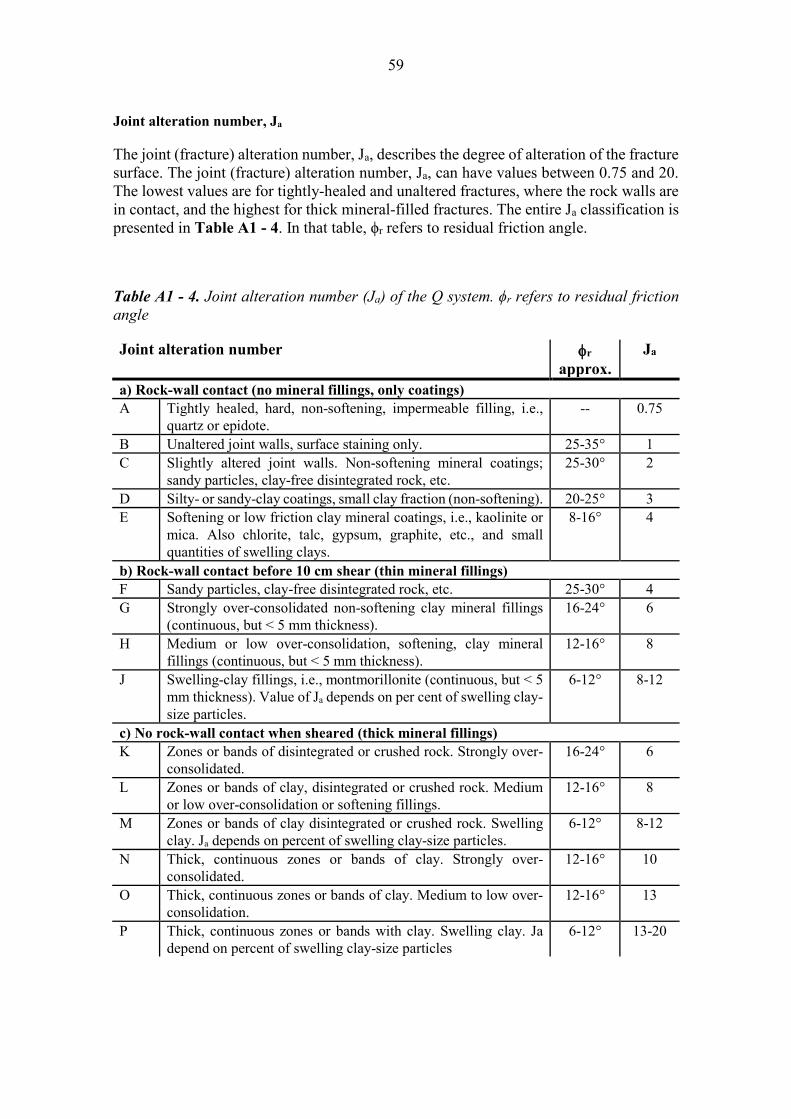
59

Joint alteration number, Ja

The joint (fracture) alteration number, Ja, describes the degree of alteration of the fracture surface. The joint (fracture) alteration number, Ja, can have values between 0.75 and 20. The lowest values are for tightly-healed and unaltered fractures, where the rock walls are in contact, and the highest for thick mineral-filled fractures. The entire Ja classification is presented in Table A1 - 4. In that table, ϕr refers to residual friction angle.

Table A1 - 4. Joint alteration number (Ja) of the Q system. ϕr refers to residual friction angle

Joint alteration number φr approx.

Ja

a) Rock-wall contact (no mineral fillings, only coatings)A Tightly healed, hard, non-softening, impermeable filling, i.e.,

quartz or epidote. -- 0.75

B Unaltered joint walls, surface staining only. 25-35° 1 C Slightly altered joint walls. Non-softening mineral coatings;

sandy particles, clay-free disintegrated rock, etc. 25-30° 2

D Silty- or sandy-clay coatings, small clay fraction (non-softening). 20-25° 3 E Softening or low friction clay mineral coatings, i.e., kaolinite or

mica. Also chlorite, talc, gypsum, graphite, etc., and small quantities of swelling clays.

8-16° 4

b) Rock-wall contact before 10 cm shear (thin mineral fillings)F Sandy particles, clay-free disintegrated rock, etc. 25-30° 4 G Strongly over-consolidated non-softening clay mineral fillings

(continuous, but < 5 mm thickness). 16-24° 6

H Medium or low over-consolidation, softening, clay mineral fillings (continuous, but < 5 mm thickness).

12-16° 8

J Swelling-clay fillings, i.e., montmorillonite (continuous, but < 5 mm thickness). Value of Ja depends on per cent of swelling clay-size particles.

6-12° 8-12

c) No rock-wall contact when sheared (thick mineral fillings)K Zones or bands of disintegrated or crushed rock. Strongly over-

consolidated. 16-24° 6

L Zones or bands of clay, disintegrated or crushed rock. Medium or low over-consolidation or softening fillings.

12-16° 8

M Zones or bands of clay disintegrated or crushed rock. Swelling clay. Ja depends on percent of swelling clay-size particles.

6-12° 8-12

N Thick, continuous zones or bands of clay. Strongly over-consolidated.

12-16° 10

O Thick, continuous zones or bands of clay. Medium to low over-consolidation.

12-16° 13

P Thick, continuous zones or bands with clay. Swelling clay. Ja depend on percent of swelling clay-size particles

6-12° 13-20

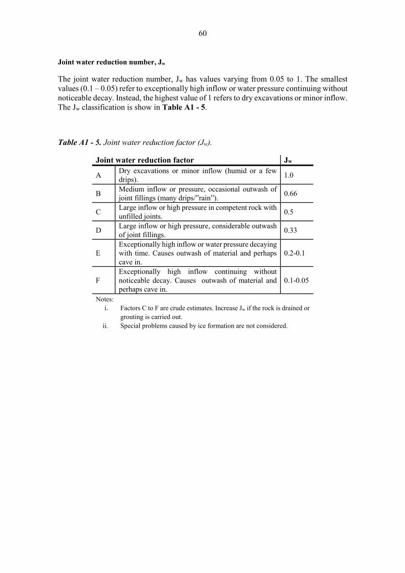
60

Joint water reduction number, Jw

The joint water reduction number, Jw has values varying from 0.05 to 1. The smallest values (0.1 – 0.05) refer to exceptionally high inflow or water pressure continuing without noticeable decay. Instead, the highest value of 1 refers to dry excavations or minor inflow. The Jw classification is show in Table A1 - 5.

Table A1 - 5. Joint water reduction factor (Jw).

Joint water reduction factor Jw

A Dry excavations or minor inflow (humid or a few drips). 1.0

B Medium inflow or pressure, occasional outwash of joint fillings (many drips/”rain”). 0.66

C Large inflow or high pressure in competent rock with unfilled joints. 0.5

D Large inflow or high pressure, considerable outwash of joint fillings. 0.33

E Exceptionally high inflow or water pressure decaying with time. Causes outwash of material and perhaps cave in.

0.2-0.1

F Exceptionally high inflow continuing without noticeable decay. Causes outwash of material and perhaps cave in.

0.1-0.05

Notes: i. Factors C to F are crude estimates. Increase Jw if the rock is drained or

grouting is carried out.ii. Special problems caused by ice formation are not considered.

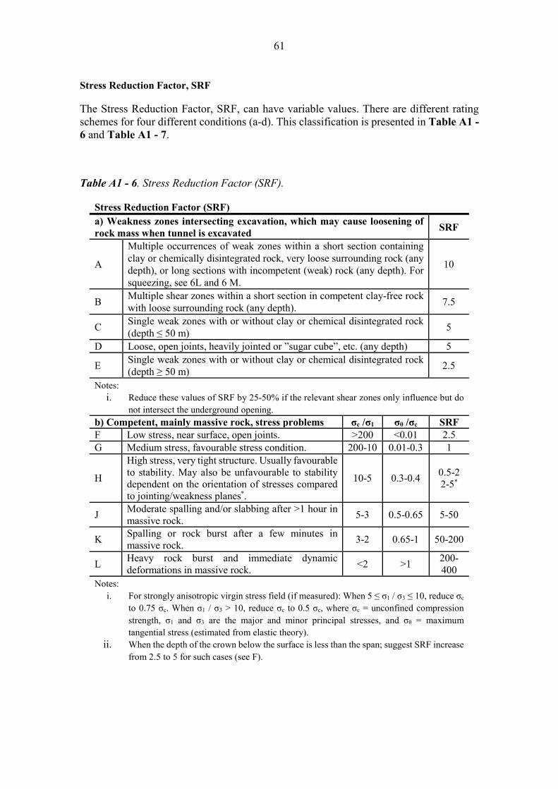
61

Stress Reduction Factor, SRF

The Stress Reduction Factor, SRF, can have variable values. There are different rating schemes for four different conditions (a-d). This classification is presented in Table A1 - 6 and Table A1 - 7.

Table A1 - 6. Stress Reduction Factor (SRF).

Stress Reduction Factor (SRF) a) Weakness zones intersecting excavation, which may cause loosening ofrock mass when tunnel is excavated SRF

A

Multiple occurrences of weak zones within a short section containing clay or chemically disintegrated rock, very loose surrounding rock (any depth), or long sections with incompetent (weak) rock (any depth). For squeezing, see 6L and 6 M.

10

B Multiple shear zones within a short section in competent clay-free rock with loose surrounding rock (any depth). 7.5

C Single weak zones with or without clay or chemical disintegrated rock (depth ≤ 50 m) 5

D Loose, open joints, heavily jointed or ”sugar cube”, etc. (any depth) 5

E Single weak zones with or without clay or chemical disintegrated rock (depth ≥ 50 m) 2.5

Notes: i. Reduce these values of SRF by 25-50% if the relevant shear zones only influence but do

not intersect the underground opening.b) Competent, mainly massive rock, stress problems σc /σ1 σθ /σc SRF F Low stress, near surface, open joints. >200 <0.01 2.5 G Medium stress, favourable stress condition. 200-10 0.01-0.3 1

H

High stress, very tight structure. Usually favourable to stability. May also be unfavourable to stability dependent on the orientation of stresses compared to jointing/weakness planes*.

10-5 0.3-0.4 0.5-2 2-5*

J Moderate spalling and/or slabbing after >1 hour in massive rock. 5-3 0.5-0.65 5-50

K Spalling or rock burst after a few minutes in massive rock. 3-2 0.65-1 50-200

L Heavy rock burst and immediate dynamic deformations in massive rock. <2 >1 200-

400 Notes:

i. For strongly anisotropic virgin stress field (if measured): When 5 ≤ σ1 / σ3 ≤ 10, reduce σc

to 0.75 σc. When σ1 / σ3 > 10, reduce σc to 0.5 σc, where σc = unconfined compressionstrength, σ1 and σ3 are the major and minor principal stresses, and σθ = maximumtangential stress (estimated from elastic theory).

ii. When the depth of the crown below the surface is less than the span; suggest SRF increasefrom 2.5 to 5 for such cases (see F).

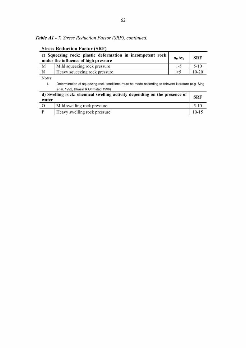
62

Table A1 - 7. Stress Reduction Factor (SRF), continued.

Stress Reduction Factor (SRF) c) Squeezing rock: plastic deformation in incompetent rockunder the influence of high pressure σθ /σc SRF

M Mild squeezing rock pressure 1-5 5-10 N Heavy squeezing rock pressure >5 10-20 Notes:

i. Determination of squeezing rock conditions must be made according to relevant literature (e.g. Singet al, 1992, Bhasin & Grimstad 1996)

d) Swelling rock: chemical swelling activity depending on the presence ofwater SRF

O Mild swelling rock pressure 5-10 P Heavy swelling rock pressure 10-15

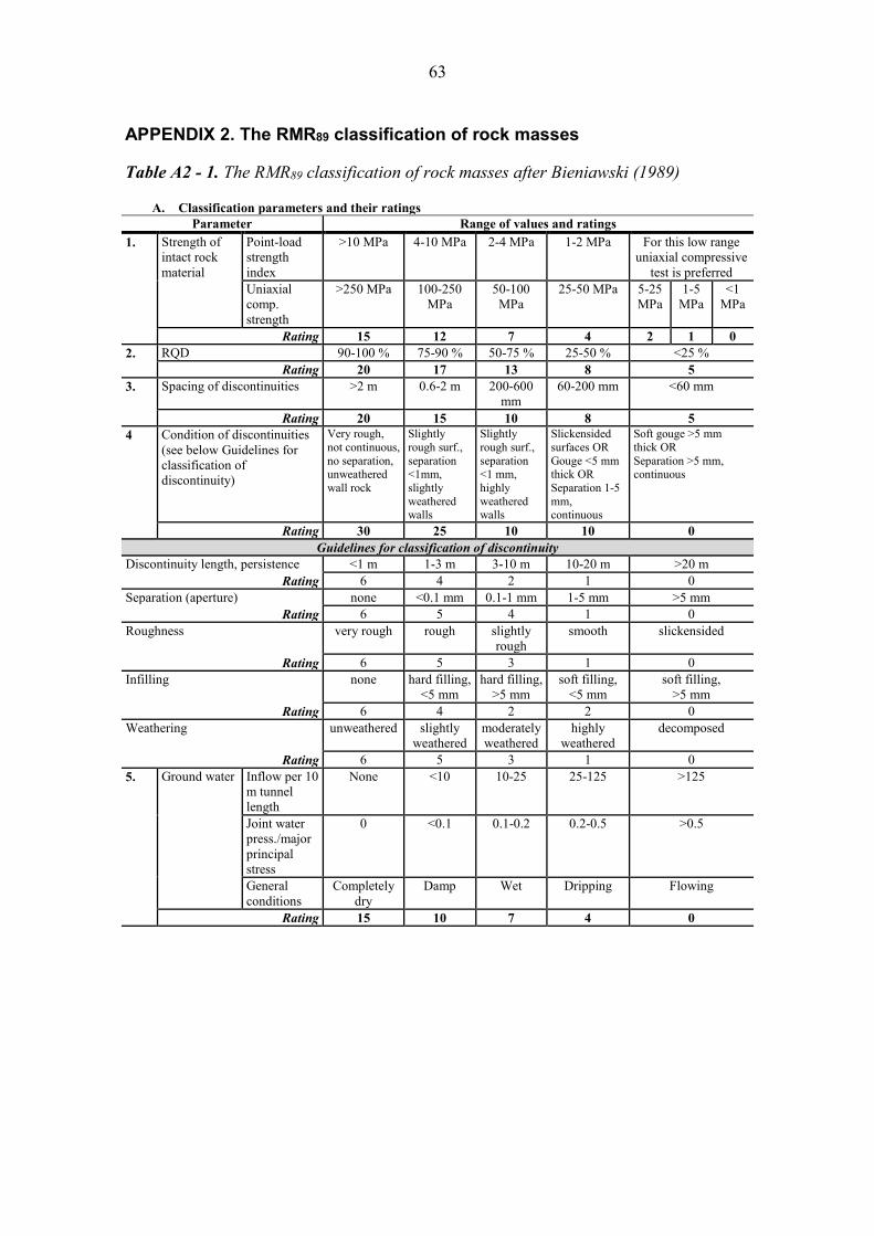
63

APPENDIX 2. The RMR89 classification of rock masses

Table A2 - 1. The RMR89 classification of rock masses after Bieniawski (1989)

A. Classification parameters and their ratingsParameter Range of values and ratings

1. Strength ofintact rockmaterial

Point-load strength index

>10 MPa 4-10 MPa 2-4 MPa 1-2 MPa For this low range uniaxial compressive

test is preferred Uniaxial comp. strength

>250 MPa 100-250MPa

50-100MPa

25-50 MPa 5-25MPa

1-5MPa

<1 MPa

Rating 15 12 7 4 2 1 0 2. RQD 90-100 % 75-90 % 50-75 % 25-50 % <25 %

Rating 20 17 13 8 5 3. Spacing of discontinuities >2 m 0.6-2 m 200-600

mm60-200 mm <60 mm

Rating 20 15 10 8 5 4 Condition of discontinuities

(see below Guidelines for classification of discontinuity)

Very rough, not continuous, no separation, unweathered wall rock

Slightly rough surf., separation <1mm, slightly weathered walls

Slightly rough surf., separation <1 mm, highly weathered walls

Slickensided surfaces OR Gouge <5 mm thick OR Separation 1-5 mm, continuous

Soft gouge >5 mm thick OR Separation >5 mm, continuous

Rating 30 25 10 10 0 Guidelines for classification of discontinuity

Discontinuity length, persistence <1 m 1-3 m 3-10 m 10-20 m >20 mRating 6 4 2 1 0

Separation (aperture) none <0.1 mm 0.1-1 mm 1-5 mm >5 mmRating 6 5 4 1 0

Roughness very rough rough slightly rough

smooth slickensided

Rating 6 5 3 1 0 Infilling none hard filling,

<5 mm hard filling,

>5 mmsoft filling,

<5 mm soft filling,

>5 mmRating 6 4 2 2 0

Weathering unweathered slightly weathered

moderately weathered

highly weathered

decomposed

Rating 6 5 3 1 0 5. Ground water Inflow per 10

m tunnel length

None <10 10-25 25-125 >125

Joint water press./major principal stress

0 <0.1 0.1-0.2 0.2-0.5 >0.5

General conditions

Completely dry

Damp Wet Dripping Flowing

Rating 15 10 7 4 0

64

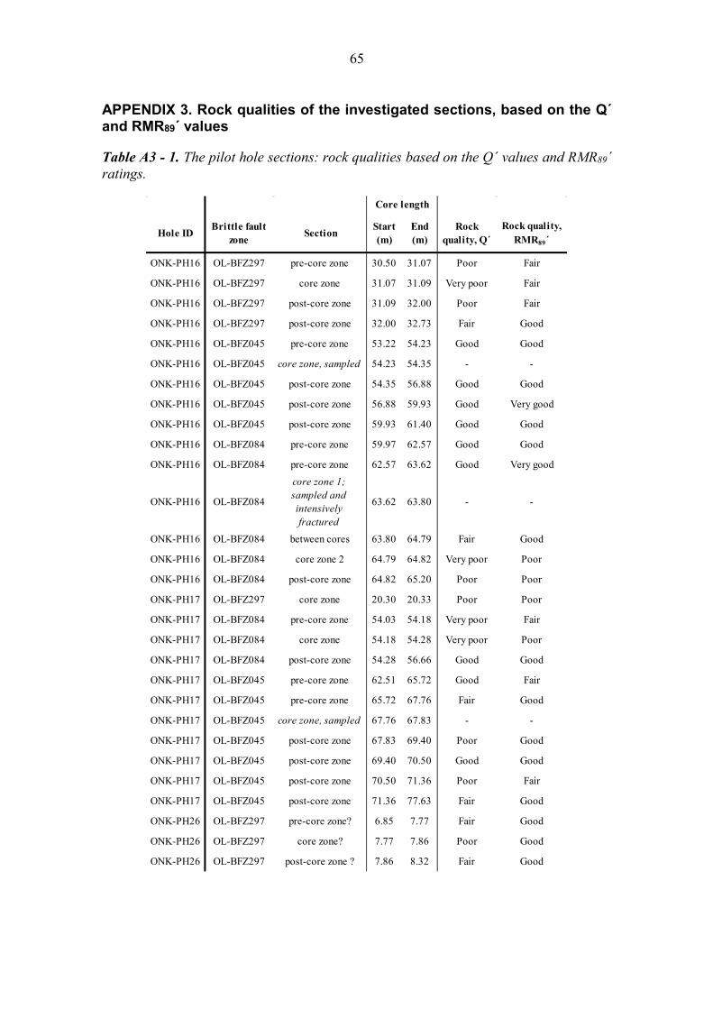
65

APPENDIX 3. Rock qualities of the investigated sections, based on the Q´ and RMR89´ values

Table A3 - 1. The pilot hole sections: rock qualities based on the Q´ values and RMR89´ ratings.

Hole ID Brittle fault zone Section Start

(m)End (m)

Rock quality, Q´

Rock quality, RMR89´

ONK-PH16 OL-BFZ297 pre-core zone 30.50 31.07 Poor Fair

ONK-PH16 OL-BFZ297 core zone 31.07 31.09 Very poor Fair

ONK-PH16 OL-BFZ297 post-core zone 31.09 32.00 Poor Fair

ONK-PH16 OL-BFZ297 post-core zone 32.00 32.73 Fair Good

ONK-PH16 OL-BFZ045 pre-core zone 53.22 54.23 Good Good

ONK-PH16 OL-BFZ045 core zone, sampled 54.23 54.35 - -

ONK-PH16 OL-BFZ045 post-core zone 54.35 56.88 Good Good

ONK-PH16 OL-BFZ045 post-core zone 56.88 59.93 Good Very good

ONK-PH16 OL-BFZ045 post-core zone 59.93 61.40 Good Good

ONK-PH16 OL-BFZ084 pre-core zone 59.97 62.57 Good Good

ONK-PH16 OL-BFZ084 pre-core zone 62.57 63.62 Good Very good

ONK-PH16 OL-BFZ084

core zone 1; sampled and intensively fractured

63.62 63.80 - -

ONK-PH16 OL-BFZ084 between cores 63.80 64.79 Fair Good

ONK-PH16 OL-BFZ084 core zone 2 64.79 64.82 Very poor Poor

ONK-PH16 OL-BFZ084 post-core zone 64.82 65.20 Poor Poor

ONK-PH17 OL-BFZ297 core zone 20.30 20.33 Poor Poor

ONK-PH17 OL-BFZ084 pre-core zone 54.03 54.18 Very poor Fair

ONK-PH17 OL-BFZ084 core zone 54.18 54.28 Very poor Poor

ONK-PH17 OL-BFZ084 post-core zone 54.28 56.66 Good Good

ONK-PH17 OL-BFZ045 pre-core zone 62.51 65.72 Good Fair

ONK-PH17 OL-BFZ045 pre-core zone 65.72 67.76 Fair Good

ONK-PH17 OL-BFZ045 core zone, sampled 67.76 67.83 - -

ONK-PH17 OL-BFZ045 post-core zone 67.83 69.40 Poor Good

ONK-PH17 OL-BFZ045 post-core zone 69.40 70.50 Good Good

ONK-PH17 OL-BFZ045 post-core zone 70.50 71.36 Poor Fair

ONK-PH17 OL-BFZ045 post-core zone 71.36 77.63 Fair Good

ONK-PH26 OL-BFZ297 pre-core zone? 6.85 7.77 Fair Good

ONK-PH26 OL-BFZ297 core zone? 7.77 7.86 Poor Good

ONK-PH26 OL-BFZ297 post-core zone ? 7.86 8.32 Fair Good

Core length

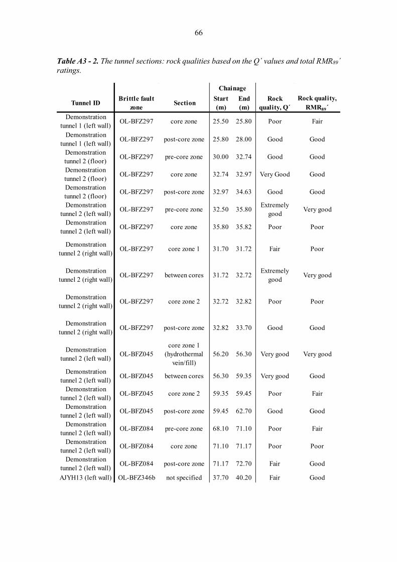
66

Table A3 - 2. The tunnel sections: rock qualities based on the Q´ values and total RMR89´ ratings.

Tunnel ID Brittle fault zone Section Start

(m)End (m)

Rock quality, Q´

Rock quality, RMR89´

Demonstration tunnel 1 (left wall) OL-BFZ297 core zone 25.50 25.80 Poor Fair

Demonstration tunnel 1 (left wall) OL-BFZ297 post-core zone 25.80 28.00 Good Good

Demonstration tunnel 2 (floor) OL-BFZ297 pre-core zone 30.00 32.74 Good Good

Demonstration tunnel 2 (floor) OL-BFZ297 core zone 32.74 32.97 Very Good Good

Demonstration tunnel 2 (floor) OL-BFZ297 post-core zone 32.97 34.63 Good Good

Demonstration tunnel 2 (left wall) OL-BFZ297 pre-core zone 32.50 35.80 Extremely

good Very good

Demonstration tunnel 2 (left wall) OL-BFZ297 core zone 35.80 35.82 Poor Poor

Demonstration tunnel 2 (right wall) OL-BFZ297 core zone 1 31.70 31.72 Fair Poor

Demonstration tunnel 2 (right wall) OL-BFZ297 between cores 31.72 32.72 Extremely

good Very good

Demonstration tunnel 2 (right wall) OL-BFZ297 core zone 2 32.72 32.82 Poor Poor

Demonstration tunnel 2 (right wall) OL-BFZ297 post-core zone 32.82 33.70 Good Good

Demonstration tunnel 2 (left wall) OL-BFZ045

core zone 1 (hydrothermal

vein/fill)56.20 56.30 Very good Very good

Demonstration tunnel 2 (left wall) OL-BFZ045 between cores 56.30 59.35 Very good Good

Demonstration tunnel 2 (left wall) OL-BFZ045 core zone 2 59.35 59.45 Poor Fair

Demonstration tunnel 2 (left wall) OL-BFZ045 post-core zone 59.45 62.70 Good Good

Demonstration tunnel 2 (left wall) OL-BFZ084 pre-core zone 68.10 71.10 Poor Fair

Demonstration tunnel 2 (left wall) OL-BFZ084 core zone 71.10 71.17 Poor Poor

Demonstration tunnel 2 (left wall) OL-BFZ084 post-core zone 71.17 72.70 Fair Good

AJYH13 (left wall) OL-BFZ346b not specified 37.70 40.20 Fair Good

Chainage

Wo

rk

ing

Re

po

rt 2

01

4-4

4 •

Re

su

lts o

f Mo

nito

ring

at O

lkilu

oto

in 2

01

3 - H

yd

rog

eo

ch

em

istry