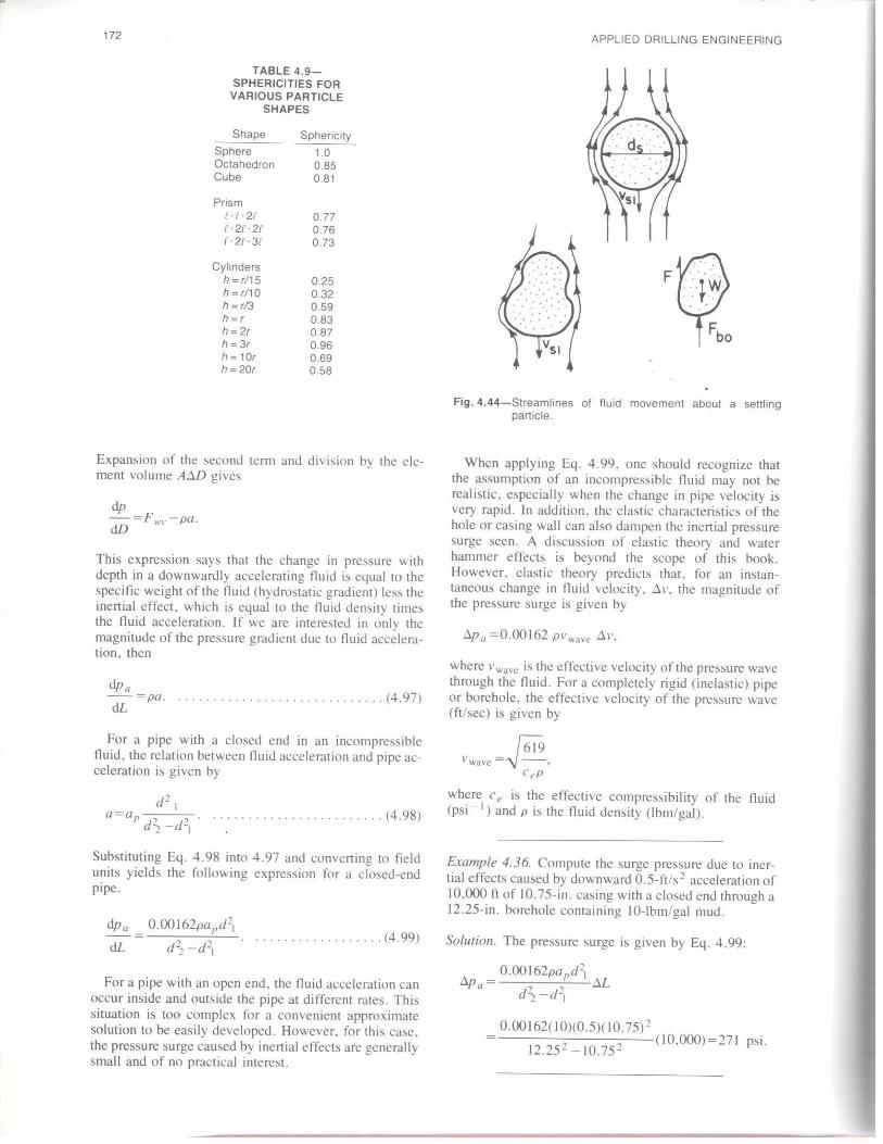
0.00162( 10)(0.5)( 1 O. 75) 2 ~ 2 (10,000)=271 psi.

12.25~­10.75

Solution. The pressure surge is given by Eq. 4.99:

Example 4.36. Compute the surge pressure dueto iner­ tial effects caused by downward 0.5­ft/s 2 acceleration of 10,000 ft of 10.75­in. casing with a closed end through a 12.25­in. borehole containing 10­lbm/gal mud.

where Vwavc is the effective velocity ofthe pressure wave through the tluid. For a completcly rigid (inelastic) pipe or boreholc, the effective velocity of thc prcssure wave (ft/sec) is given by

l'wave=fe, CeP

where e e is the effective compressibility of the fluid (psi ­ I) and p is the fluid density (lbm/gal) .

Sp¿ =0.00162 PVwa,c 111',

When applying Eq. 4. 99. one should recognize that the assumption of an incompressible fluid may not be realistic. especially when the change in pipe velocity is very rapid. In addition, the elastic characteristics of the hole or casing wall can also dampen the inertial pressure surge seen. A discussion of elastic theory and water hammer effects is beyond the scope of this book. However, elastic theory predicts that, for an instan­ taneous change in fluid velocity, /11•, the magnitude of the pressure surge is given by

Fig. 4.44-Streamlines of fluid movement about a settling particle.

F

APPLIED DRILLING ENGINEERING

For a pipe with an open end , the fluid acceleration can occur inside and outside the pipe at different rates. This situation is too complex for a convenient approximate solution to be easily developed. However, for this case, the pressure surge caused by inertial effects are generally small and of no practica! intcrcst.

0.00162paPd21 ----'--. . ( 4. 99)

d22 -d21

Substituting Eq. 4.98 into 4.97 and converting to field units yields the following expression for a closed­cnd pipe.

. . . . . . . . . . . . . . . . . . . . . . . . (4.98)

For a pipe with a closed end in an incompressible fluid, the relation betwcen fluid acceleration and pipe ac­ celeration is given by

dpa -=pa (4.97) dL

This expression says that thc change in pressure with depth in a downwardly accelerating fluid is equal to the specific weight of the fluid (hydrostatic gradient) lcss thc inertial effect, which is cqual to the fluid density times the fluid acceleration. lf we are interested in only the magnitude of the pressure gradient due to fluid accelera­ tion, then

dp -=Fw .. -pa. d.D

Expansion of the second tenn and division by the ele­ ment volume A!iD gives

0.25 0.32 0.59 0.83 0.87 0.96 0.69 0.58

Cylinders h = r/15 h=r/10 h=r/3 h =r h=2r h=3r h= 10, h=20r

0.77 0.76 0.73

Prism f · f · 2f t'· 2f · 2f f · 2f · 31'

Sphere Octahedron Cube

Sphericity 1.0 0.85 0.81

Shape

TABLE 4.9- SPHERICITIES FOR

VARIOUS PARTICLE SHAPES

172

24 !=- (4.105) NRe

The proof of this relation is left as an exercise .

This equation can be extended to Reynolds numbers below 0.1 if the friction factor at low Reynolds number is defined by

~ d5 (Pi -p¡) 04d ,,, ~1.89 .! ~ (4.1 )

f=3.57 d,2 (Ps -p¡). . (4.104c) Vsl PJ

Solving this equation for the particle slip velocity yields

4 d, P., =o¡ f=-g--- (4.104b) 3 v.,12 PJ

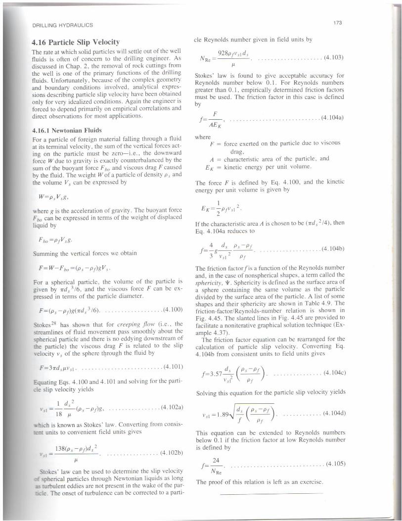
The friction factor f is a function of the Reynolds number and, in the case of nonspherical shapes, a tenn called the sphericity, '1r. Sphericity is defined as the surface area of a sphere containing the same volume as the particle divided by the surface area of the particle. A list of sorne shapes and their sphericity are shown in Table 4.9. The friction­factor/Reynolds­number relation is shown in Fig. 4.45. The slanted lines in Fig. 4.45 are provided to facilitate a noniterative graphical solution technique (Ex­ ample 4.37) .

The friction factor equation can be rearranged for the calculation of particle slip velocity. Converting Eq. 4.104b from consisten! units to field units gives

1 ~ E K = - P ¡v s 1 - ·

2 If the characteristic area A is chosen to be ( 1rd/ !4), then Eq. 4.104a reduces to

The force F is defined by Eq. 4.100, and the kinetic energy per unit volume is given by

where F = force exerted on the particle due to viscous

drag, A = characteristic area of the particle, and

E K = kinetic energy per unit volume.

F !=-, (4.104a) AEK

928p¡Vs1d1 NRe = (4.103)

µ,

Stokes' law is found to give acceptable accuracy for Reynolds number below 0.1. For Reynolds numbers greater than O. 1, empirically detennined friction factors must be used. The friction factor in this case is defined by

ele Reynolds number given in field units by

173

................ (4.102b) 138(p5 -p¡)d/

'•• = µ,

Str-kes law can be used to determine the slip velocity pherical particles through Newtonian liquids as long

.zs rarbulent eddies are not present in the wake of the par­ e. The onset of turbulence can be corrected to a partí­

l d 2 =IB¿(p5-p¡)g, (4.102a)

ich is known as Stokes' law. Converting from consis­ tmt units to convenient field units gives

Equating Eqs. 4. 100 and 4.101 and solving for the parti­ de slip velocity yields

F=37íd5µ,v51 ••••••••••••..•••••••••••• (4.101)

Smkes28 has shown that for creeping flow (i.e., the sireamlines of fluid movement pass smoothly about the .pherical particle and there is no eddying downstream of

tne particle) the viscous drag F is related to the slip veíociry v s of the sphere through the fluid by

F=(p s -p ¡)g( -n d s 3 /6). . (4. 100)

For a spherical particle, the volume of the particle is grven by ttd¿ 3 /6, and the viscous force F can be ex­ pressed in tenns of the particle diameter.

F= W-Fbo =t», -p¡)gV,.

Summing the vertical forces we obtain

where gis the acceleration of gravity. The buoyant force F bo can be expressed in tenns of the weight of displaced liquid by

4.16.1 Newtonian Fluids For a particle of foreign material falling through a fluid at its terminal velocity, the sum of the vertical forces act­ mg on the particle must be zero­i .e., the downward force W due to gravity is exactly counterbalanced by the sum of the buoyant force F bo and viscous drag F caused by the fluid. The weight W of a particle of density p s and the volume V, can be expressed by

4.16 Particle Slip Velocity The rate at which sol id particles will settle out of the well fluids is often of concem to the drilling engineer. As discussed in Chap. 2, the removal of rock cuttings from the well is one of the primary functions of the drilling fluids. Unfortunately, because of the complex gcometry and boundary conditions involved , analytical expres­ sions describing particle slip velocity have been obtained only for very idealized conditions. Again the engineer is forced to depend primarily on cmpirical correlations and direct observations for most applications.

DRILLING HYDRAULICS

Fig. 4.45-Friction factors for compunnq particle-slip velocity: (a) crushed sohds and spheres and (b) particles of difieren! sphencttíes.

cr o .... u ~

z o ..... u cr LL

10,000 ~ " " " " " " \ )ffl~~+~~_:,:_:i~_,H\,__\­­~­:\~;_..,­+­_~\:­\~_:,:­~~~\,_\­­­+­+'_,l:+'t­t,+­+­t­­+­,~\~~\~~~~~~~~~;:~;:~;!~~~~~~!::!

1000~=t:Eí52E'"~ii=l=\E:l~Eí=\EEEl!i=E\=il~E\=ilIDat=EEE=E=EEEÉ=E=EE 600 1­\. ' ' ' ' , , 400r'-\t-~,H+~'d-+-~~~N11o~'*+~',--~'H+~'ltl-+'+t-1r-v-'-H't-tt-~'.i--+-+tt-+-+-++r-+--+-H 200~\+--i-+-\c'-+- \ 'f0lM~._...H+--+\~~~~\--I--H'.+-~\.....+--+~~4\~-14~~~+--+---+-+-1

100 \ \ '~ ~ ~~ \ \ \ , \ 60~t--1rt-H+-\+'---tr+H~'rt-~~--~~.....,...+++~"+--ft-t-++-'''r+---ft-H+-~'---tr+++--+-+-+++--t--~ \ \ \ \ '\: ,lo ~ ... \ \ \ \ \ \ 4 o t­­­,r­­­­,Pll­i­+­'1.t­Pr++­­\t­­+\l"i+"'\J"­~lil'"+.c=­'l­­+*+r­­\f­­4~~~+lt­++­~ , , . = o. 1 2 e _,_,_ 20 \ ' \ ~, ~;;:: - ~ \ w 1

10 ~ \ \ ~ "~1"~ ~~""' \ \ tµ=0.220 __ ,_ 6 \. \.. ' '\. """'­­ ' '\ ' 1 --i---

4 t­­­,!­­­1H­t+­\t­ '­­+''~­'\t­­­+l\­\1­+t­­\t­'~'.i­­~Pk­­',~+""­~1­~~­~ ... , i­++­~',.._..,..;'~"' = o. 600- - .- 2 ' " , ' '~... ~ ........ """' ' ' -lJ!=0.806 _

\ \ ' \ \r­.. \ \ 1\l 111 1 1 ~=1S=ll:=Ea*·=EE~"~=tma"=1*~·*l=~,s;i:l:at~·'.1"' = 1.000=== 0.4~~1-=+l+=+=~"Jíl~'~4'~~~',+==~"¡¡¡3\~~,~~'\J=~~~~~,;¡::~"~~::::t~"~~I::¡::~ g~ ::=::::=:::::=:\=::":=~\=:~:\=~1:\:~:~~11.~\~~ ....... \'\I- ...... +--~l.\-\~~:'~=:\~~:':=:-:::-

0. 001 0.01 0.1 1 2 4 10 100 1000 10,000 105 106 PARTICLE REYNOLDS NUMBER,

BASE O ON DI A METER OF EQUIVALENT SPHERE (b)

LL

~ cr ~ u ~

z o .... u a: LL

0.01 0.1 1 2 4 10 100 1000 10,000 105 106 REYNOLDS NUMBER. BASED ON AVERAGE SCREEN SI ZE

(a)

1000

288 200 100

~8 20 10 ~ 2

1 0.6 0.4 0.2 0.1

0.001 PARTICLE

LL

'. ... ' ' ' ' \ ' ' ' ' ' ' "'I \ ' \ ' ' \ \ \ \ \ ~ ~I\ \ \ ~ 1\ ~ ' \ ~" ~ " Crushed Si lica ~ \ \

' ,... ­... ' • ' • ' ' ' ... ' a ' " ' ' ' \ , \ ~ ~ \ \1 \1 \ ' \ \ \ S >heres~ ~ -crushed Galena

, ' ' ' ' \ \ N ~ \ 11 \ \ \ \ \ '­ \ \ \ \

\ \ \ \ ,¡ \ \ \ \ \ \ \ 1\ 1\ ' t- ' \ ' ~ ~ ' \

\ \ ' ... \'r­.. \ \ \ ' ' ' ' ' \ ' \ ' \ ,. \ ......... \ ' ' \ \ \

' - , l

, \ ' \ \ 11. \ ~ ...... ~ ......

\ \ ~ \ \ ...... "" \ \ \ ' \ \ \ \ ­ \ \

\ \ \ \ \ \ \ \ , \ \ \

' ' \ 11. l \ ~ \ \ \

\ \ \ \ \ \ ­ \

10,000

APPLIED DRILLING ENGINEERING 174

=0.038 in.

10.4(2.6(8.33)­9.0]

5 T d = g s

10.4(p5 -p¡)

Solution. The maximum diameter of a spherical sand grain is given by Eq. 4.106c:

Example 4.38. Compute the rnaximum­diarneter sand particle having a specific gravity of 2.6 that can be suspended by a mud that has a density of 9 lbm/gal anda gel strength of 5 lbm/ 100 sq ft.

to settle through a fluid having gel strength r 8. Particles having a diameter slightly greater than that

given by Eq. 4.106c will settle slowly such that the flow pattem around the sphere corresponds to creeping flow. An analytical solution for creeping flow has not been developed for non­Newtonian fluids.

T d , = g ..•.........••...•... (4.106c)

10.4(p s -p ¡)

or, conversely, the particle diameter must exceed

r8=10.4d5(ps-PJ), (4.106b)

Converting this equation from consistent units to field units gives

ds r8=-(p5-p¡), (4.106a)

6

Thus, the gel strength r 8 needed to suspend a particle of diameter d, is given by

4.16.2 Non-Newtonian Fluids Particles will not settle through a static non­Newtonian fluid unless the net force on the particle due to gravity and buoyancy is sufficient to overcome the gel strength of the fluid. For a sphere, the surface area is 1rd5

2, and the force required to break the gel is equal to nd s 2 t e: Equating this force to the net force given by Eq. 4.100 gives

303 (O. O I ) = 5 ft. (1­0.4)

porosity of 0.40, the fill on bottom is approximately

175

of the bottom portion of the hole. If the sand packs with a

30(10.1)=303 ft

If circulation is stopped for 30 minutes. the sand will set­ tle from approximately

=0.17 ft/s or 10. l ft/min.

/ 0.025 12.6(8.33)­(8.33)J =l.89....J­­­­­­­­

5 8.33

V5¡ = 1.89~ ds (P, -p¡) f P¡

Entering Fig. 4.45a at the point (f=0.108, NRe =222) and moving parallel to the slant lines to the curve for '1'=0.81 yields an intersection point (!=5, NRc=40). Thus, the slip velocity is given by

=222.

928p ¡V si d s 928(8.33)( l. J 5)(0.025) N Re = ----'---

µ

and

=0.108,

3 .57[2.6(8. 33)­8.33)0.025

8.33(1.15)2

3.57(p5-p¡)d, J=------'-- 2 PJVs¡

This slip velocity corresponds to a friction factor and Reynolds number given by

= 1.15 ft/s.

µ

138(2.6(8.33)­8.33](0.025) 2

138(p5 -p¡)ds 2

v a=

Solution. A slip velocity first must be assumed to establish a point on the friction factor plot shown in Fig. 4.45. Assuming Stokes' law is applicable,

Example 4.37. How much sand having a mean diameter of0.025 anda sphericity of0.81 will settle to the bottom of the hole if circulation is stopped for 30 minutes. The drilling fluid is 8.33­lbm/gal water having a viscosity of 1 cp and containing about l % sand by volume. The specific gravity of the sand is 2.6.

DRILLING HYDRAULICS

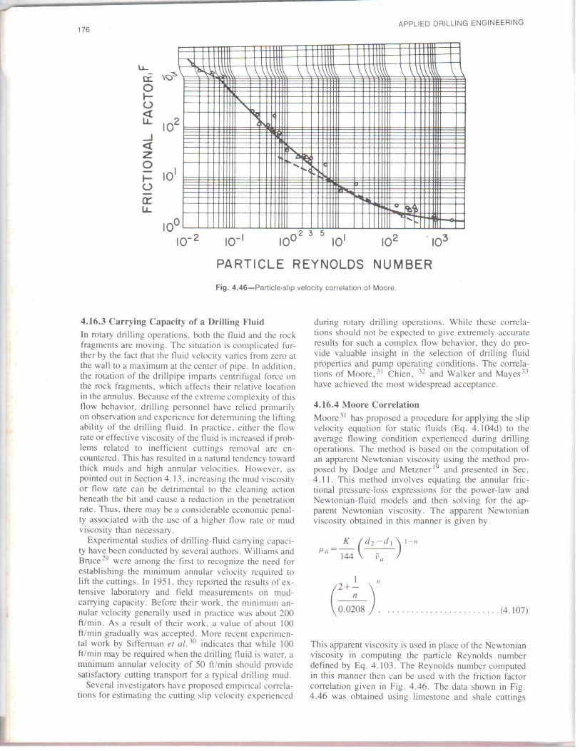
This apparent viscosity is used in place of the Newtonian viscosity in computing the particle Reynolds number defined by Eq. 4.103. The Reynolds number computed in this manner then can be used with the friction factor correlation given in Fig. 4.46. The data shown in Fig. 4.46 was obtained using limestone and shale cuttings

........................ (4.107) (2+~ )"

o.o:os .

_ K (d2­d1) 1­11 P..a --- -

144 l'a

4.16.4 Moore Correlation Moore31 has proposcd a procedure for applying the slip velocity equation for static fluids (Eq. 4.104d) to the average flowing condition experienced during drilling operations. The method is based on the computation of an apparent Newtonian viscosity using the method pro­ posed by Dodge and Metzner19 and presented in Sec. 4. 11. This method involves equating the annular frie­ tional pressure­loss expressions for the power­law and Newtonian­fluid models and then solving for the ap­ parent Newtonian viscosity. The apparent Newtonian viscosity obtained in this manner is given by

during rotary drilling operations. While these correla­ tions should not be expected to give extremely accurate results for such a complex flow behavior, they do pro­ vide valuable insight in the selection of drilling fluid properties and pump operating conditions. The correla­ tions of Moore, 31 Chien, 32 and Walkcr and Maycs33 have achicvcd the most widespread acceptance.

4.16.3 Carrying Capacity of a Drilling Fluid In rotary drilling operations, both the fluid and the rock fragments are moving. The situation is complicated fur­ ther by the fact that the fluid velocity varíes from zero at the wall to a maximum at the center of pipe. In addition, the rotation of the drillpipe imparts centrifuga! force on the rock fragrnents, which affects their relative location in the annulus. Beca use of the extreme complexity of this flow behavior, drilling personnel have relied primarily on observation and experience for detennining the lifting ability of the drilling fluid. In practice. either the flow rate or effective viscosity of the fluid is increased if prob­ lems related to inefficient cuttings removal are en­ countered. This has resulted in a natural tendency toward thick muds and high annular velocities. However, as pointed out in Section 4.13. increasing the mud viscosity or flow rate can be detrimental to the cleaning action beneath the bit and cause a reduction in the penetration rate. Thus , there may be a considerable economic penal­ ty associated with the use of a higher flow rate or mud viscosity than necessary.

Experimental studies of drilling­fluid carrying capaci­ ty have been conducted by severa! authors. Williams and Bruce29 wcre among the first to recognize the need for establishing the minimum annular velocity required to lift the cuttings. In 1951. they reported the results of ex­ tensive laboratory and field measurements on mud­ carrying capacity. Before their work , the minimum an­ nular velocity gcnerally used in practice was about 200 ft/min. As a result of their work , a value of about 100 ft/min gradually was accepted. More recent experimen­ tal work by Siffennan et al. 30 indicates that while 100 ft/min may be required when the drilling fluid is water, a minimum annular velocity of 50 ft/min should provide satisfactory cutting transport for a typical drilling mud.

Severa! investigators have proposed empirical correla­ tions for estimating the cutting slip vclocity experienced

Fig. 4.46-Particle-slip velocity correlation of Moore.

PARTICLE REYNOLDS NUMBER

\\ \ \

1 1 1

\

1 "1 1 11111 \.L.

a: o ..... u ~ _J <{ z o ..... u a:: u,

1 1 1 11 1TT

.\\\\\\ 1 1 1 11111 11111 11111

\ \

111 111 ill

APPLIED ORILLING ENGINEERING 176

~J36,800d~ (Ps-Pf)+I -l] ( ...!!:!!._) p f

p¡ds

.......................... (4.110)

v si =0.0075 ( ...!!:!!._) P¡ds

However, for suspensions of bentonite in water, rt is recommended that the plastic viscosity be used for the apparent viscosity. For particle Reynolds numbers above 100, Chien recommends the use of 1.72 for the friction factor. This is only slightly higher than the value of 1.5 recommended by Moore. For Jower particle Reynolds numbers, the following correlation was presented:

Ty d, µa =µp +5­_­. . (4.109)

Va

4.16.5 Chien Correlation The Chien correlation 32 is similar to the Moore correla­ tion in that it involves the computation of an apparent Newtonian viscosity for use in the particle Reynolds number determination. For polymer­type drilling fluids, Chien recommends computing the apparent viscosity using

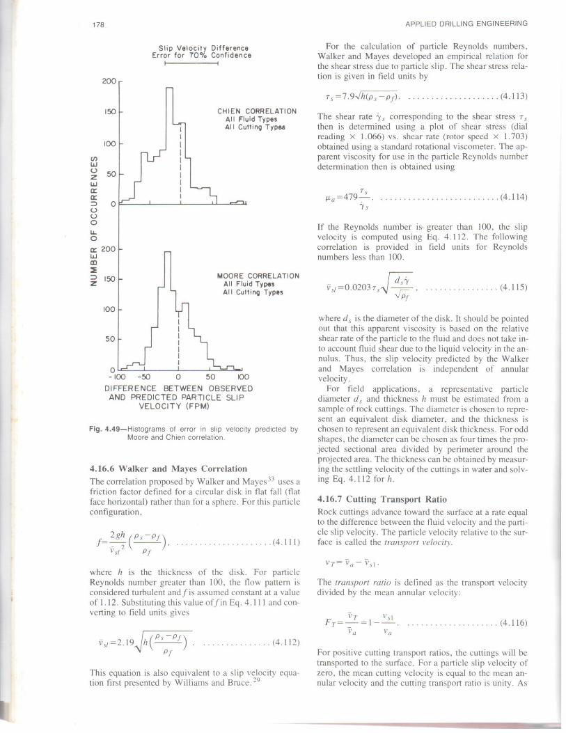
Fig. 4.48-Histograms of error in cuttings-transport ratio predictions by various methods.

­200 ­150 ­100 ­50 O 50 100 150 200 250

PERCENT ERROR IN PREDICTEO CUTTING TRANSPORT RATIO

WALKER ANO MAYES CORRELATION

MOORE CORRELATION

CHIEN CORRELATION

NEW TECHNIQUE

Non-Newton,an Flu1ds

40 30

20

10

11) o w 40 (.) z w 30 Q: Q: 20 :::> (.) 10 o o o u. o 40 Q: 30 w a:,

20 :,¿ :::> 10 z

o 40

30

20

10

o ­250

Tronsport Rot,o Prediction Percent Error For 70% Conl1dence ,..._._.., 10.0

177

............. (4.108c)

For this relation, the slip velocity equation reduces to

22 !=-- .¡¡;¡;;: .

For intermediate Reynolds numbers, the dashed line ap­ proximation shown in Fig. 4.46 is given by

d 2 V5¡ =82.87­5­(p5 -p¡). . (4.108b)

J.La

For this condition, the slip velocity equation reduces to

40 !=-.

NRe

For particle Reynolds numbers of 3 or less, the flow pat­ tem is considered to be laminar and the friction factor plots as a staight line such that

This corresponds to a transitional flow pattem between laminar flow and fully developed turbulent flow.

~ p =»¡ V5¡=1.54d5-5-- •..•••....•...... (4.108a) Pf

from field drilling operations. For Reynolds numbers greater than 300, the flow around the particle is fully tur­ bulent and the friction factor becomes essentially con­ stan! at a value of about 1.5. For this condition, the slip velocity (Eq. 4.104d) reduces to

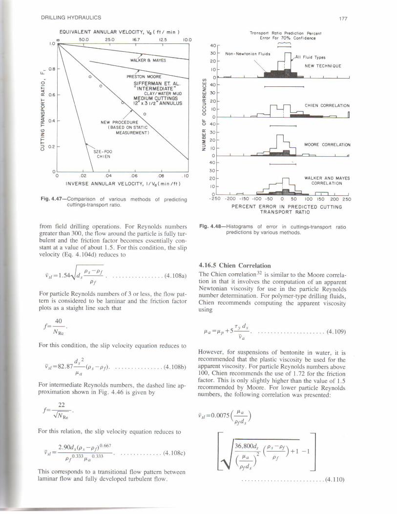
Fig. 4.47-Comparison of various methods of predicting cuttings-transport ratio.

O O .02 .04 .06 .08 . 10

INVERSE ANNULAR VELOCITY, I/V0( min /ft)

SZE-FOO CHIEN

NEW PROCEOURE ( 8ASEO ON STATIC

MEASUREMENT)

o

PRESTON MOORE

SIFFERMAN ET. AL. "INTERMEOIATE"

CLAY / WATER MUO MEDIUM CUTTINGS 12" x 3 112" ANNULUS

o

_ 0.8 u.

­ o ¡::: et Q: 0.6 1­ Q:

~ 11) z ~ 0.4 1­ (!) z 1­ 1­ :::> 0.2 o

12.5 16.7 25.0 50.0 EOUIVALENT ANNULAR VELOCITY, Va ( ft I min )

DAILLING HYDAAULICS

For positive cutting transport ratios. the cuttings will be transported to the surface. For a particle slip velocity of zero, the mean cutting velocity is equal to the mean an­ nular velocity and the cutting transport ratio is unity. As

vT v_,1 F7=­=­­=I­­ (4.116)

Va v"

The transport ratio is defined as the transport velocity divided by the mean annular velocity:

1'7= 1'a ­ v.d ·

4.16.7 Cutting Transport Ratio Rock cuttings advance toward the surface at a rate equal to the difference between the fluid velocity and the parti­ cle slip velocity. The particle velocity relative to the sur­ face is called the transport velocity.

where d, is the diameter of the disk. It should be pointed out that this apparent viscosity is based on the relative shear rate of the particle to the fluid and does not take in­ to account fluid shear dueto the liquid velocity in the an­ nulus. Thus, the slip velocity predicted by the Walker and Mayes correlation is independent of annular velocity.

For field applications, a representative particle diameter d , and thickness h must be estimated from a sample of rock cuttings. The diameter is chosen to repre­ sent an equivalen! disk diarneter, and the thickness is chosen to representan equivalen! disk thickness. For odd shapes, the diameter can be chosen as four times the pro­ jected sectional area divided by perimeter around the projected area. The thickness can be obtained by measur­ ing the settling velocity of the cuttings in water and solv­ ing Eq. 4.112 for h.

v51=0.0203r.,~, (4.115) "PJ

lf the Reynolds number is greater than 100, the slip velocity is computed using Eq. 4.112. The following correlation is provided in field units for Reynolds numbers less than 100.

Ts µ0 =479­. . (4.114)

'Y s

The shear rate ~ s corresponding to the shear stress r s then is deterrnined using a plot of shear stress (dial reading X 1.066) vs. shear rate (rotor speed x 1. 703) obtained using a standard rotational viscometer. The ap­ parent viscosity for use in the particle Reynolds number deterrnination then is obtained using

r5=7.9)h(p5-p¡) (4.113)

For the calculation of particle Reynolds nurnbers, Walker and Mayes developed an empirical relation for the shear stress dueto particle slip. The shear stress rela­ tion is given in field units by

APPLIED DRILLING ENGINEERING

This equation is also equivalen! to a slip velocity equa­ tion first presented by Williams and Bruce. 29

where h is the thickness of the disk. For particle Reynolds number greater than 100. the flow pattem is considered turbulent andf is assumed constant ata value of 1.12. Substituting this value off in Eq. 4.111 and con­ verting to field units gives

!= 2-g~ (P, -p¡), , (4.111) v»: Pf

4.16.6 Walker and Mayes Correlation The correlation proposed by Walker and Mayes33 uses a friction factor defined for a circular disk in tlat fall (flat face horizontal) rather than for a sphere. For this particle configuration,

Fig. 4.49-Histograms of error in slip velocity predicted by Moore and Chien correlation.

o '-=-.....L----Ji----L--==-...!oal

- 100 -50 O 50 IOO OIFFERENCE BETWEEN OBSERVEO ANO PREOICTED PARTICLE SLIP

VELOCITY (FPM)

MOORE CORRELATION AII Fluid Types AII Cuttino Types

CHIEN CORRELATION AII Fluld Types Al I Cuttino Typea

200

150

100

(/) w u 50 z UJ cr: cr: :::> o u u o LL o cr: 200 w (X)

~ ::> 150 z

100

50

Slip Velocity Difference Error for 70% Confidence

178

transport ratio could be obtained. This procedure was ap­ plied using data obtained in full­scale experiments by Sifferman et al., and the results are shown in Fig. 4.47. The correlations of Moore, Chien, and Walker and Mayes also were applied, and the results are plotted in Fig. 4.47 for comparison. Note that the method of Sam­ ple and Bourgoyne gave the best results for this example. Note also that the experimental data as well as the com­ puted results obtained with the various correlations gave essentially a straight­line plot.

Sample and Bourgoyne compiled a computer data file containing all the available published experimental data on cuttings slip velocity in flowing fluids. The data file consists of measurements obtained for different fluid types (water, polymer, and clay muds) using a variety of particle types and sizes (spheres, disks, rectangular prisms, and actual rock cuttings). The data file was used to evaluate the accuracy of the various methods for predicting cuttings transport ratio. The error histograms are shown in Fig. 4.48. The most accurate approach was found to be the use of an experimental slip velocity

16.2 150

16.3

16.4 => o w w .....J o ~ ~ g ..... o CD

(!) 16.8 a.. a..

> ..... en

16.7 2 w o (!) 2

16.6 ~ .....J => o a:: (.)

16.5 .,_ 2 w .....J ~

179

the slip velocity increases, the transport ratio decreases and the concentration of cuttings in the annulus en route to the surface increases. Cutting transport ratio is, thus, an excellent measure of the carrying capacity of a par­ ticular drilling fluid.

In recent work by Sample and Bourgoyne, 34 a plot of transport ratio vs. the reciproca! of the annular velocity was found to be an extremely convenient graphical tech­ nique. As can be seen from Eq. 4.116, if slip velocity is independent of annular velocity, a straight­line plot should result. The slope of the line is numerically equal to the particle slip velocity, and the x intercept is equal to the reciproca! of the particle slip velocity. The y in­ tercept, which corresponds to an infinite annular veloci­ ty, must be equal to a transport ratio of one. Sample and Bourgoyne found that for annular velocities below about 120 ft/min, the slip velocity was essentially independent of annular velocity. Thus, by making an experimental determination of slip velocity in a static column and then drawing a line from the y intercept of 1.0 to the x intercept of l!v s » an approximate representation of cutting

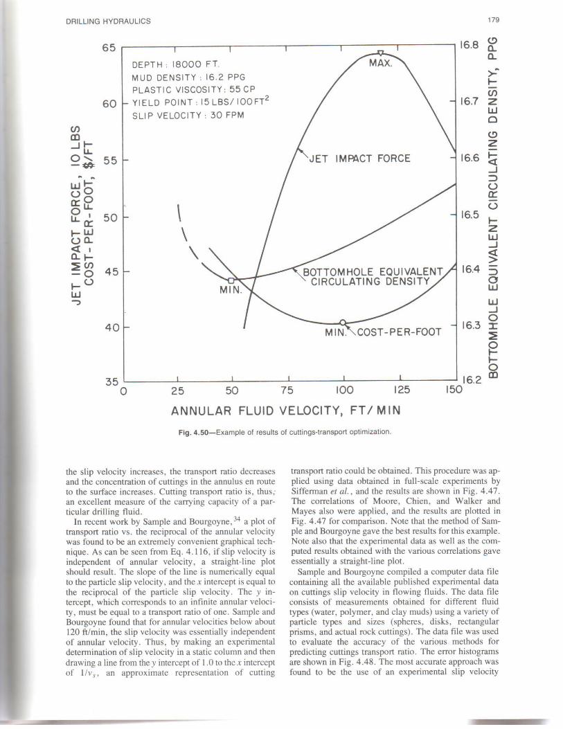
Fig. 4.50-Example of results of cuttings-transport optimization.

ANNULAR FLUID VELOCITY, FT I M IN

100 125 75 35 L-~~___J'---~~___J'---~~~.1...-~~~.l...-~~~...L.-~~----J

o 50 25

JET IMPACT FORCE

40

45

50

55

DEPTH: 18000 FT. MUD DENSITY: 16.2 PPG PLASTIC VISCOSITY: 55 CP YIELD POINT: 15 LBS/ IOOFT2

SLIP VELOCITY: 30 FPM

\ \ \

60

DRILLING HYDRAULICS

where A b is the area cut by the bit. This equation assurnes that the cuttings do not disintegrate to the size of individual grains. Otherwise, a factor of ( 1-</>) rnust be

dD q,=Abdt (4.117)

For low values of cuttings transport ratio, the concen­ tration of cuttings in the annulus is high, causing a high effective rnud density. This in turn causes a high cir­ culating bottornhole pressure and a low penetration rate.

The volurne fraction of cuttings in the rnud can be deterrnined by considering the feed rate , q .1, of cuttings at the bit, and the cuttings transport ratio, F T· For a given bit penetration rate , (dD/dt), the feed rate of cut­ tings is

rneasurerncnt rnadc in a rccently stirred static sarnple of thc drilling fluid. Thc rnost accuratc crnpirical corrcla­ tion was found to be that of Moore. 31 A slip velocity er­ ror histograrn for the Moore correlation is shown in Fig. 4.49.

Sarnple and Bourgoyne34 also developed a cornputcr rnodel for estirnating the optima] cuttings transport ratio for a given set of field conditions. The cornputer rnodel predicts the cost per foot usi ng Eq. 1 . 16 presented in Sec. 1. 1 O of Chap. 1. The penetration rate was predicted using the drilling rnodel defined by Eq. 5.28 presented in Sec. 5.7 of Chap. 5. Thc penetration rate equation assurnes an exponential decline in penetration rate with increasing bottomhole pressure. It also assurnes that penetration rate increases proportionally to the jet irnpact force raised to the 0.3 power.

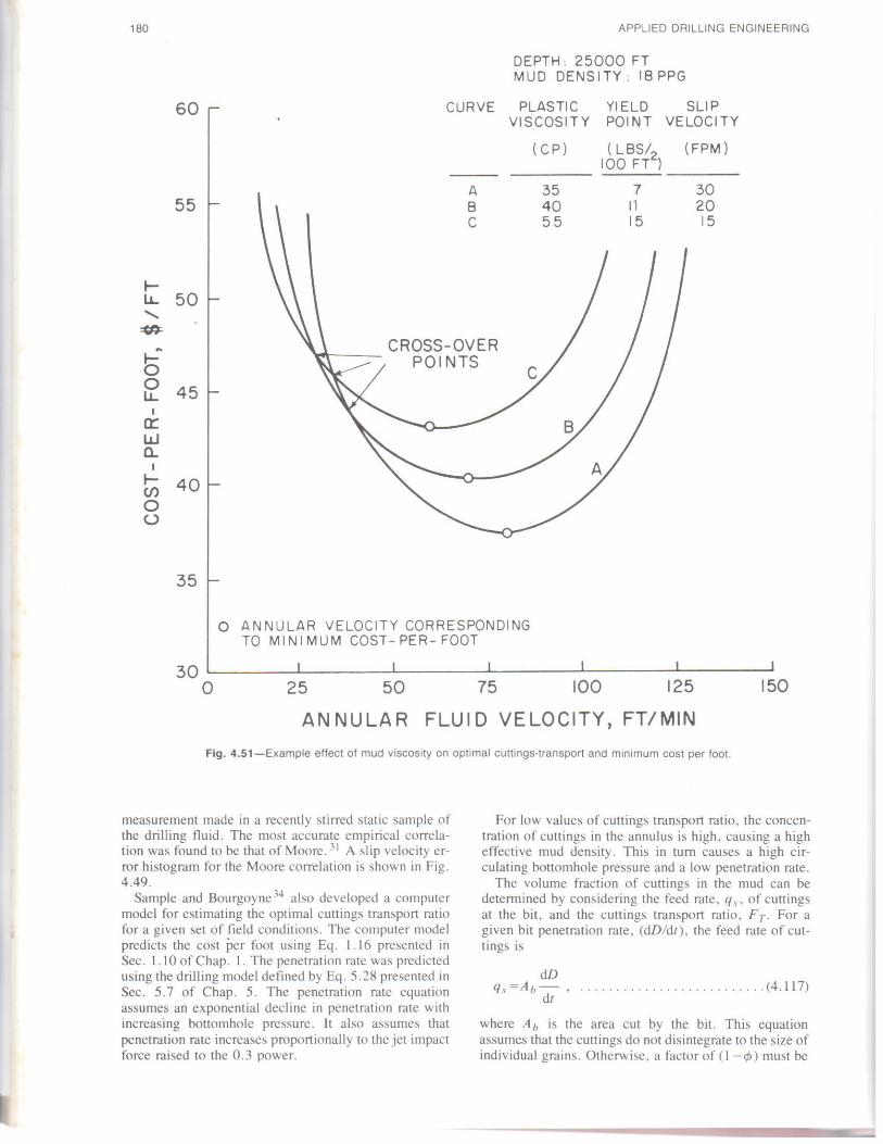
Fig. 4.51-Example effect of mud viscosity on optima! cuttings-transport and mínimum cost per foot.

ANNULAR FLUID VELOCITY, FT/MIN

30 L.-~~~L._~~~..,L._~~~--1....-~~~-'--~~~-'-~~~---' O 25 50 75 100 125 150

O ANNULAR VELOCITY CORRESPONDING TO MINI MU M COST - PE R- FOOT

35

1- LL 50 <,

~

~

CROSS-OVER POINTS

o 45 LL 1

a:: w a..

1 1- 40 en o (..)

180 APPLIED DRILLING ENGINEERING

DEPTH: 25000 FT MUO DENSITY: 18 PPG

60 CURVE PLASTIC YIELD SLIP VISCOSITY POINT VELOCITY

( C P) ( LBS/ (FPM) 100 FT2)

A 35 7 30 55 8 40 11 20

e 55 15 15

=58 cp.

= 152 ( 10­s)o.26(2+110.74)º·74 144 2 0.0208

The apparent Newtonian viscosity at an annular velocity of 120 ft/min (2 ft/s) is given by Eq. 4.107

510 (30) K= 074 =152 eq cp.

511 ·

n=3.32 log(:~) =0.74.

Solution. Moore Correlation The consistency index K and flow behavior index n based on the 300­ and 600­rpm reading normally are used with the Moore correlation.

Assume both the diameter and thickness of the cuttings are approximately 0.25 in.

2.0 3.3

13 22 30 50

3 6

100 200 300 600

Dial Reading (degree)

Rotor Speed (rpm)

Example 4.39. Compute the transport ratio of a 0.25­in. cutting having a specific gravity of 2.6 (21.6 lbm/gal) in a 9.0­lbm/gal clay/water mud being pumped at an an­ nular velocity of 120 ft/min (2.0 ft/s) in a 10x5 in. an­ nulus. Apply the correlations of Moore, Chien, and Walker and Mayes. The following data were obtained for the drilling fluid using a rotational viscometer.

Exceptions to this rule are seen primarily for shallow, large­diameter boreholes, where the theoretical minimum cost per foot occurs to the left of the crossover region shown in Fig. 4.51. Of course, the drilling fluid must serve many other functions not considered in the cost per foot formula, and the drilling fluid viscosity used is often a result of many considerations. For exarn- ple, it may be impossible to achieve a low­viscosity drill­ ing fluid and simultaneously maintain a high fluid densi­ ty which may be required to prevent a blowout.

181

where p s is the average density of the cuttings. The average density of the mud in the annulus can be

decreased by increasing the mud flow rate and thus in­ creasing the transport ratio. However, as the mud flow rate is increased, a point is reached at which bottomhole pressure begins increasing with increasing flow rate due to excessive frictional pressure losses in the annulus. Also the jet impact force available at the bit begins to decrease with increasing flow rate due to the excessive frictional pressure losses in the drillstring. Thus , there exists an optima! flow rate which results in a minimum theoretical cost per foot.

Typical results obtained using the computer model of Sample and Bourgoyne are shown in Fig. 4.50 for a 16.2­lbm/gal mud having a plastic viscosity of 40 cp, a yield point of 15, anda cuttings slip velocity of 30 ft/min while drilling an 8.5­in. hole at 18.000 ft. Note that the mínimum theoretical cost per foot occurred atan annular velocity of 100 ft/min. The maximum impact force oc­ curred at an annular velocity of 120 ft/min and the mínimum equivalen! circulating density occurred at an annular velocity of 50 ft/min. For most drilling condi­ tions studied, the maximum impact force criteria tended to yield only slightly higher costs per foot than the true optimum.

Cuttings transport ratio can be increased by increasing the annular fluid velocity or by adjusting the fluid prop­ erties such as viscosity or density. In most cases, a lower theoretical cost per foot could be achieved through the use of low­viscosity fluids. Example results computed for muds of varying viscosity are shown in Fig. 4.51.

p=pm( 1­f.v) +p sÍv , · · · · (4. 119)

Once the volume fraction of cuttings is known, the effec­ tive annular mud density , p, can be computed using

....................... (4.118) f - q, s-

q,\ +Frqm

Solving this expression for the volume fraction gives

qm

q,

Aafv Fr=-----

where f, is the volume fraction of cuttings in the mud and q,,, is the flow rate of the mud.

Since the transpon ratio. F r- is defined as 1·r/1·0•

then

Aa(l -f,) q/11

applied, where cj) is the rock porosity. The transport velocity of the cuttings, vr- and fluid, v O. in a borehole annulus of area A0 is given by

DRILLING HYDRAULICS

928(9)(1.07)(0.25) NRc= =57.

39

/ o.25c,. 103)( 1 oo> =0.0203(14)­­J J9 = 1.07 ft/s.

The particle Reynolds number for this slip velocity is given by

rr: v.1 =0.0203 T s--.,J Fp

Assuming a transitional tlow pattern, the slip velocity is given by Eq. 4.115.

14 µ0 =479 =39 cp.

( l. 703)( 100)

This, in tum, corresponds roughly to a rotor specd of 100 rpm for the data given. The shear rate at the bob in the Fann viscometer is l. 703 times the rotor specd. Thus, we have

14 ­­=13.1. 1.065

A shear stress of 14 lbm/100 sq ft corresponds to a Fann dial reading given by

= 14.0 lbm/100 sq ft.

Ti =7.9Jh(ps-Pf)

=7. 9J0.25(2 l.6­9.0)

Walker and Mayes Correlation The shear stress of the particle falling in a static liquid is estimated using Eq. 4.113.

2.0­0.79 F T= =0.605 or 60.5%.

2.0

Since this Reynolds number is less than 100, the use of Eq. 4.110 is justified. The transpon ratio is given by

= 928(9)(0.25) = 82 5 NRe 20 ..

The particlc Reynolds number for this slip velocity is given by

=0.79 ft/s.

36,800(0.25) (21.6­9) J +I-1 (8.89)2 9

v1¡ =0.0075(8.89)

thcn

APPLIED DRILLING ENGINEERING

µ ?O (Pf;s) = 9(;.25) =8.89'

Sin ce

i\¡=0.0075( ~) p¡d\

Assuming a transitional flow pattern, the slip velocity is given by Eq. 4.110:

µP =50­30=20 cp.

Chien Correlation For clay/water muds. Chien recommends thc use of thc plastic viscosity as the apparent viscosity. Using the 300­ and 600­rpm rcadings on thc Fann gives

2.0­0.49 FT= =0.755or75.5%.

2.0

928p¡ \.\¡d, 928(9)(0.49)(0.25) NRc = = = 18.

µll 58

Since this Reynolds number is between 3 and 300. the use of Eq. 4.108c is justified. The transpon ratio for an annular velocity of 2.0 ft/s anda cutting slip vclocity of 0.49 ft/s is given by

The particle Reynolds number is given by

2. 9(0.25)(21.6­9 .O)º 667 ­­­­­­­­­=0.49 ft s. 90 333580.331

Assuming an intermediare particle Reynolds number (transitional tlow pattem). the slip velocity i\ given by Eq. 4.108c:

2. 90d\ (p 1 -p¡)º 667

v a= P O 333µ 0.333 f ll

Fig. 4.52-Example fluid columns for Exerc,se 4.1.

(o) ( e ) ( b)

Grovel Sp Gr •2 61 Poros,ty•0.3

IOpp9

10'10 10,000'

182

4.10 A well is being drilled ata vertical depth of 12,200 ft while circulating a 12­lbm/gal mud ata rate of 9 bbl/min when the well begins to flow. Fifteen bar­ reis of mud are gained in the pit over a 5­minute period before the pump is stopped and the blowout preventers are closed. After the pressures stabil­ ized, an initial drillpipe pressure of 400 psia and an initial casing pressure of 550 psia were recorded. The annular capacity opposite the 5­in .. 19 .5­lbf/ft drillpipe is 0.0775 bbl/ft. The annular capacity op­ posite the 600 ft of 3­in. ID drill collars is 0.035 bbl/ft. Assume M= 16 and T=600ºR.

a. Compute the density of the kick material assuming the kick entered as a slug. Answer: 5.28 lbrn/gal.

b. Compute the density of the kick material assuming the kick mixed with the mud pumped during the detection time. Answer: 1.54 lbm/gal.

c. Do you think that the kick is a liquid ora gas? d. Compute the pressure that will be observed at

4.9 A massive gas sand at 10,000 ft having a porosity of 0.30 and a water saturation of 0.35 is being drilled at a rate of 80 ft/hr using a 9.875­in. bit. The drilling mud has a density of 12 lbm/gal and is being circulated at a rate of 400 gal/min. The an­ nular capacity is 2.8 gal/ft. The mean temperature of the well is 600ºR. Ignore the slip velocity of the gas bubbles and rock cuttings.

a. After steady­state conditions are reached, what is the effective bottomhole pressure? Assume that the gas is pure methane and behaves as an ideal gas. Answer: 6,205 psia.

b. What is the equivalent mud weight in the an­ nulus? Answer: 11.9 lbm/gal.

c. What is the mud density of the mud leaving the annulus at the surface at atmospheric pressure? Answer: 5.8 lbm/gal.

d. Make a plot of the density of the drilling fluid in the annulus vs. depth.

e. Can the gas­cut mud at the surface be eliminated completely by increasing the mud densi­ ty? Answer: no.

4.8 The penetration ratc of the rotary drilling process can be increased greatly by lowering the hydrostatic pressure exerted against the hole bot­ tom. In areas where formation pressures are con­ trolled easily, the effective hydrostatic pressure sometimes is reduced by injecting gas with the well fluids. Calculate the volume of methane gas per volume of water (standard cubic feet per gallon) that rnust be injected at 5,000 ft to lower the effec­ tive hydrostatic gradient of fresh water to 6.5 lbm/gal. Assume ideal gas behavior andan average gas temperature of 174 ºF. Neglect the slip velocity of the gas relative to the water velocity. Answer: O. 764 scf/gal.

d. If formation brine of specific gravity 1.1 enters the annulus up to a depth of 11,000 ft before the blowout preventers are closed, what will be the surface annular pressure after the well is shut in? Answer: 231 psig.

183

4.7 A well is being drilled at 12,000 ft using an 11­lbm/gal mud when a permeable formation hav­ ing a fluid pressure of 7 ,000 psig is cut by the bit.

a. If fluid circulation is stopped, what hydrostatic pressure will be exerted by the mud against the permeable formation? Answer: 6,864 psig.

b. Will the well flow if the blowout preventers are left open? Answer: yes.

c. Calculate the surface drillpipe pressure if the blowout preventers are closed. Answer: 136 psig.

4.6 A casing string is to be cemented in place ata depth of 10,000 ft. The well contains 10­lbm/gal mud when the casing string is placed on bottom. The cementing operation is designed so that the 10­lbm/gal mud will be displaced from the annulus by (1) 500 ft of 8.5­lbm/gal mud flush, (2) 2,000 ft of 12.7­lbm/gal filler cement, and (3) 1,500 ft of 16.7­lbm/gal high­strength cement. The high­ strength cement will be displaced from the casing by 9­lbm/gal brine. Calculate the mínimum pump pressure required to completely displace the casing. Assume no shoe joints are used. Answer: 1,284 psig.

4.5 A well contains methane gas occupying the upper 6,000 ft of annulus. The mean gas temperature is 170ºF and the surface pressure is 4,000 psia.

a. Estímate the pressure exerted against a sand below the bottom of the surface casing at a depth of 5,500 ft. Assume ideal gas behavior. Answer: 4,378 psia.

b. Calculate the equivalent density at a depth of 5,500 ft. Answer: 15.3 lbm/gal.

4.4 The mud density of a well is being increased from 10 to 12 lbm/gal. If the pump is stopped when the interface between the two muds is at depth of 8,000 ft in the drillstring, what pressure must be held at the surface by the annular blowout preventers to stop the well from flowing? What is the equivalent density in annulus at 4,000 ft after the blowout pre­ venters are closed? Answer: 832 psig, 14 lbm/gal.

4.3 An ideal gas has an average molecular weight of 20. What is the density of the gas al 2,000 psia and 600ºR? Answer: 0.8 lbm/gal.

4.2 Calculate the mud density required to fracture a stratum at 5,000 ft if the fracture pressure is 3,800 psig. Answer: 14.6 lbm/gal.

Exercises 4. l Calculate the hydrostatic pressure at the bottom of

the fluid column for each case shown in Fig. 4.52. Answer: 5,200 psig for Case A.

Since this Reynolds number is less than 100, the use of Eq. 4.115 is justified. The transport ratio is given by

2.0­1.07 F7= =0.465 or 46.5%.

2.0

DAILLING HYDAAULICS