Embed Size (px)
Citation preview

Growth, Specialisation, and Economic Integration in Europe
by
Mercedes Vera-Martin, London School of Economics
Submitted to the University of London in partial fulfillment of the requirements for the degree of
PhD. in Economics
at the
UNIVERSITY OF LONDON
September 2003
© University of London 2003
Signature of A uthor...............................................................................................University of London
September 2003
Accepted by

UMI Number: U185752
All rights reserved
INFORMATION TO ALL USERS The quality of this reproduction is dependent upon the quality of the copy submitted.
In the unlikely event that the author did not send a complete manuscript and there are missing pages, these will be noted. Also, if material had to be removed,
a note will indicate the deletion.
Disscrrlation Publishing
UMI U185752Published by ProQuest LLC 2014. Copyright in the Dissertation held by the Author.
Microform Edition © ProQuest LLC.All rights reserved. This work is protected against
unauthorized copying under Title 17, United States Code.
ProQuest LLC 789 East Eisenhower Parkway
P.O. Box 1346 Ann Arbor, Ml 48106-1346

I 5
r

G row th , S p ecia lisa tion , and E conom ic In tegra tion in E urope
byMercedes Vera-Martin, London School of Economics
Submitted to the University of London on September 2003, in partial fulfillment of the
requirements for the degree of PhD. in Economics
A b stra ct
This thesis contributes to the understanding of the economic effects of European integration, on both the pattern of industrial specialisation in European regions and openness and income for countries of the European Economic Conununity (EEC).
Chapter 2 provides a descriptive analysis of the evolution of the patterns of specialisation across European regions during 1975-1995. We find that regions are more specialised than countries. Over time, countries and regions have increased specialisation, although at a slow pace. When analysing specialisation dynamics, mobility within the pattern of specialisation changes notably at the regional level. We also find significant cross-country and within- country differences in specialisation.
Chapter 3 studies production patterns in 45 European regions since 1975. We estimate a structural equation derived directly from the Heckscher-Ohlin theory, which relates an industry ’s share of a region’s GDP to factor endowments and relative prices. Factor endowments are found to play a significant and quantitatively important role. The explanation is most successful for aggregate industries, and works less well for disaggregated industries within the manufacturing sector. We find no evidence that increasing European integration has weakened or stengthened the relation between factor endowments and production patterns.
Chapter 4 adds economic geography considerations into the analysis of patterns of specialisation in manufacturing industries across regions in seven European countries since 1985. We estimate an equation that relates an industry’s share of GDP to factor endowments, industry characteristics, and economic geography variables. Both factor endowments and economic geography are found to be significant in explaining specialisation. Among economic geography variables, cost linkages are more important than demand linkages. There is no evidence that increasing integration has weakened or stengthened the relationship between factor endowments, economic geography, and production patterns within countries.
Chapter 5 explores how European economic integration has affected openness and income. We test for permanent effects of EEC membership on openness, income, and income convergence at the time of accession. Results indicate EEC membership improves permanently openness within the EEC and income, but has neither an effect on income growth nor on convergence. Second, we investigate the differential effect of EEC membership by applying a differences in differences specification which controls for common time series shock. Openness, income, and convergence among the EEC countries were improved significantly.
Chapter 1 presents an overview of the thesis with a summary of conclusions and contributions. Chapter 6 summarises the main findings of the thesis.

Contents
1 A n Overview o f the Thesis 13
1.1 In troduction .................................................................................................................. 13
1.2 Historical Background: Steps towards European Integration ........................... 14
1.3 Economic Integration and the Location of I n d u s t r y ........................................... 16
1.4 Description of T h e s is .................................................................................................. 19
1.5 Results and C o n trib u tio n s ........................................................................................ 21
2 Industrial Specialisation in European Regions 26
2.1 In troduction .................................................................................................................. 26
2.2 Related Literature ..................................................................................................... 30
2.3 A Measure of Specialisation from the Neoclassical T heory ................................. 33
2.4 Empirical Modelling of Specialisation Dynamics . ........................................... 35
2.5 Data D esc rip tio n ........................................................................................................ 37
2.6 Localisation and Specialisation in Europe: Some Summary S tatistics.............. 39
2.6.1 Industry Localisation in E u ro p e ................................................................. 40
2.6.2 Specialisation across E u ro p e ....................................................................... 41
2.7 Changes in Specialisation at the Country Level: A D ecom position................. 45
2.8 Dynamics of Patterns of S pecia lisa tion .................................................................. 47
2.9 C onclusions.................................................................................................................. 52
2.10 Appendix 2A ............................................................................................................... 88
3 Factor Endowm ents and Production in European Regions 90
3.1 In tro d u c tio n ^ ............................................................................................................... 90
As certified at the beginning of the thesis, this chapter is based on a co-joint research with my supervisor, Dr. Stephen Redding from the London School of Economics.
3

3.2 Related Literature .................................................................................................... 94
3.3 Theoretical Fram ew ork.............................................................................................. 96
3.4 Data D esc rip tio n ....................................................................................................... 102
3.5 Econometric S pecifica tion ....................................................................................... 104
3.6 Empirical R e su lts ....................................................................................................... 106
3.7 C onclusions................................................................................................................. 113
3.8 Appendix 3A .............................................................................................................. 127
3.9 Appendix 3 B .............................................................................................................. 128
3.9.1 B l. Regional-level Data on Production and E ndow m ents..................... 128
3.10 Appendix 3 C .............................................................................................................. 130
4 Factor Endowm ents, Econom ic Geography, and Specialisation in European
Regions 132
4.1 In troduction ................................................................................................................. 132
4.2 Related Literature .................................................................................................... 134
4.3 The m o d e l.................................................................................................................... 137
4.4 Data D esc rip tio n ....................................................................................................... 140
4.4.1 Regional C h arac teristics .............................................................................. 140
4.4.2 Industry C h arac te ris tics .............................................................................. 142
4.4.3 Region-Industry In teractions........................................................................ 143
4.5 Empirical R e su lts ....................................................................................................... 145
4.5.1 Estimation R e s u l ts ........................................................................................ 145
4.5.2 Prediction E r r o r s ........................................................................................... 148
4.6 C onclusions................................................................................................................. 150
4.7 Appendix A ................................................................................................................. 158
4.8 Appendix B ................................................................................................................. 159
4.8.1 B l. Regional-level Data on Production and E ndow m ents......................... 159
4.8.2 B2. Industry Characteristics........................................................................ 159
5 M em bership in European Econom ic Community, O penness, and Growth 161
5.1 In troduction ................................................................................................................. 161
5.2 Steps to European Integration: Some Historical B ack g ro u n d ......................... 164

5.3 Related Literature ................................................................................................. 166
5.4 The m o d e l.................................................................................................................... 170
5.5 Permanent Effects of EEC M em bership.................................................................. 172
5.6 Differential Effects of EEC M embership.................................................................. 176
5.7 C onclusions................................................................................................................ 179
6 C onclusions 187

List of Tables
2.1 Shares of Agriculture, Manufacturing, and Services in GDP (percent) . . . . 55
2.2 Shares of the Disaggregated Manufacturing Industries in GDP in France and
Spain (p e rc e n t) ........................................................................................................... 57
2.3 Evolution of the Goefficient of Variation for the One-Digit Sectors, at the
Gountry and Regional Levels.................................................................................... 59
2.4 Evolution of the Goefficient of Variation for the Manufacturing Industries, at
the Country and Regional Levels ........................................................................... 60
2.5 (cont) Evolution of the Coefficient of Variation for the Manufacturing Indus
tries, at the Gountry and Regional Levels.............................................................. 61
2.6 Matrix of Correlation of the Pattern of Specilisation across Countries, Manu
facturing In d u strie s ..................................................................................................... 62
2.7 Correlation Matrices of the Pattern of Specialisation for the Regions within
the same G oun try ........................................................................................................ 63
2.8 Correlation Matrices of the Pattern of Specialisation for the Belgian and Span
ish Regions .................................................................................................................. 69
2.9 Krugman Indices for the Aggregated Industries, 1980-95 70
2.10 Krugman Indices for the Disaggregated Manufacturing Industries ............... 71
2.11 Annual Averages for Total Change, and. Actual Within- and Between-Region
Changes in Specialisation for the Aggregated Industries, 1975-94 (in percentage) 72
2.12 Total Change (in percentage), and Proportional Within- and Between-Region
Changes for the Disaggregated Manufacturing Industries, 1980-1995 ............. 73
2.13 (cont.) Total Change (in percentage) and Proportional Within and Between-
Region Changes for the Manufacturing Industries, 1980-1995 .......................... 73
2.14 Transition Probabilities Matrices for Belgium, Shares of GDP 5-year transitions 74

2.15 Transition Probabilities Matrices for Spain, Shares of GDP 5-year transitions 75
2.16 Transition Probabilities Matrices for France, Shares of GDP 5-year transitions 76
2.17 Transition Probabilities Matrices for Italy, Shares of GDP 5-year transitions 77
2.18 Transition Probabilities Matrices for Luxembourg and Netherlands, Shares of
GDP 5-year tran sitio n s ..................................................................................... 79
2.19 Transition Probabilities Matrices for United Kingdom, Shares of GDP 5-year
tran sitio n s ........................................................................................................... 80
2.20 Transition Probabilities, Relative Shares of GDP 5-year transitions, Gountry
Level A nalysis..................................................................................................... 82
2.21 Regional Mobility Indices Relative to Corresponding Gountry Indices, 5-year
tran sitio n s ........................................................................................................... 83
2.22 Gross-country Differences in Specialisation Dynamics, 5-year transitions . . . 84
2.23 Within-country Differences in Specialisation Dynamics, 5-year transitions . . 85
2.24 Sample C o m p o sitio n ........................................................................................ 88
2.25 Industry Composition........................................................................................ 88
2.26 Regions Included in the S a m p le ..................................................................... 89
3.1 Factor Endowments in 1975, 1985, and 1995^“^ ........................................... 115
3.2 Educational Attainment by Region in 1985 and 1995 (percentage of total
p o p u la tio n ) ........................................................................................................ 117
3.3 Factor Endowments and Specialisation in A g ricu ltu re ....................................... 118
3.4 Factor Endowments and Specialisation in M anufac tu ring ................................ 119
3.5 Factor Endowments and Specialisation in Serv ices............................................. 120
3.6 Factor Endowments and Specialisation at the Aggregate L e v e l ........................ 121
3.7 Factor Endowments and Specialisation at the Aggregate Level (Long Differ
ences) 122
3.8 Average Shares of Sectors in GDP and Within-sample Average Absolute Pre
diction E r r o r s 123
3.9 Within-sample Average Absolute Prediction Errors over T i m e ................124
3.10 Within-sample Average Absolute Prediction Errors (PE (ALT2)) in the Dis
aggregated Manufacturing Industries over T i m e 125

3.11 Within-sample Average Absolute Prediction Errors (PE (ALT2)) in the Dis
aggregated Manufacturing Industries over T i m e ................................................. 126
3.12 Sample C o m p o sitio n ................................................................................................ 127
3.13 Industry Composition................................................................................................ 127
3.14 Factor Endowments and Specialisation at the Disaggregate Level.................. 130
3.15 Factor Endowments and Specialisation at the Disaggregate Level.................. 131
4.1 OLS Regression Results, pooled observations, all manuf. industries .............. 151
4.2 (cont) OLS Regression Results, pooled observations, all manuf. industries . . 152
4.3 Robustness Analysis with Industry Dummies, All Manuf. In d u strie s ............ 153
4.4 Robustness Analysis by Clustering Observations, All Manuf. Industries . . . 154
4.5 Average Within-sample Prediction Errors Over Time, all Manuf. Industries . 155
4.6 Average Within-sample Prediction Errors Over Time, by In d u s try ............... 156
4.7 Average Within-sample Prediction Errors Over Time, by In d u s try ............... 157
4.8 Sample C o m p o sitio n ................................................................................................ 158
4.9 Industry Composition..................................................................................... 158
4.10 Industry C h a rac te ris tic s ............................................................................... 160
4.11 Industry Characteristics ( c o n t . ) .................................................................. 160
4.12 Industry Characteristics ( c o n t . ) .................................................................. 160
5.1 EEC M em bership...................................................................................................... 181
5.2 Change in the Intercept in the Series of Overall O penness................................ 182
5.3 Change in the Intercept in the Series of EEC O p en n ess................................... 182
5.4 Change in the Intercept in the Series of GDP (log) .......................................... 183
5.5 Change in the Intercept in the Series of Per-Capita GDP ( lo g ) ...................... 183
5.6 Change in the Intercept in the Series of GDP Growth R a t e s ......................... 184
5.7 Change in the Intercept in the Series of Relative G D P ...................................... 184
5.8 Differences in Differences Analysis; EEG G o u n tr ie s .......................................... 185
5.9 Differences in Differences Analysis: EEG 12 Gountries except those joining in
1973 (Denmark, Ireland and U K ) .......................................................................... 185
List o f Figures
2-1 Specialisation at a Point in T i m e .......................................................................... 86
2-2 Specialisation Dynamics 1, Increased S pecia lisa tion ........................................... 87
2-3 Specialisation Dynamics 2, Decreased Specialisation........................................... 87
5-1 Structural Break with no Scale E ffe c t..................................................................... 186
5-2 Structural Break with Scale E f fe c ts ........................................................................ 186

Certification of Co-joint WorkChapter 3 “Factor Endowments and Production in European Regions” is based on a
co-joint endeavor with my supervisor, Dr. Stephen Redding from the London School of Eco
nomics. In this regard, I was involved as a full co-author in the paper on which this chapter
is based, including the formulation of theoretical hypotheses to be tested, the development
of the empirical strategy, the construction of the dataset, the econometric estimation, and
the interpretation of the empirical results. The joint research is published as a Centre for
Economic Policy and Research discussion paper, no. 3755 (January 2003), London.
10

AcknowledgmentsW ithout the unstinting support of many friends and colleagues, I would not have been
able to complete this thesis. I am particularly grateful to my supervisors, Professor Danny
Quah and Dr. Stephen Redding for their many hours in supervising and guiding me through
this project. Special appreciation must be extended to Dr. Redding not only for his excellent
supervision, but for his unfailing encouragement and enduring accessibility, always offering
interesting and insightful conunents which often prompted long discussions. Financial sup
port from the Central Bank of Spain is gratefully acknowlegded.
During the Ph.D. program, I was associated with two excellent institutions—the London
School of Economics and the Centre for Economic Performance at the University of Lon
don, where I was able to work with excellent researchers in the areas of international trade
and geography. Among those deserving special attention were Henry Overman, Anthony
Venables, and Alan Winters. Others at the Centre who I especially would thank are partic
ipants to the weekly International Trade workshop organised by the Globalisation Group. I
am also very grateful to my colleagues, Sandra Bulli, Tushar Poddar, Lupin Rahman, and
Merxe Tudela. In addition, I extend my appreciation to participants at the 2003 Summer
Meeting of the Econometric Society in Northwestern University of Chicago for conunents to
my research in the area of economic geography in European regions. I am also grateful to
Professor Ben-David for providing support with the test formulation used in Chapter 5.
During the many years of work on this thesis, many friends were instrumental in providing
support and encouragement, often at great distance, helping me keep a wise perspective
on the work at hand. Arno, Brian, Clara, Jesper, and M arta will always be especially
remembered. I am also most grateful to Johannes for his patience and unconditional support.
Finally, in these critical years, my college professors. Dr. Enrique Martin Quilis and Dr. Juan
Aguirre played a vital role in their interest in my progress, and I want to express my great
thanks to them.
Finally, this thesis would not have been completed without the encouragement of Carlos
Medeiros, the Division Chief of the International Monetary Fund’s Capital Financing group.
In the end, I send my most special thanks to my parents, my most significant backers,
whose understanding and continued support carried me through a very demanding period
in my life. Responsibility for any results lies with the author alone.
11

A mis padres, Juan y Mercedes
12

Chapter 1
An Overview of the Thesis
1.1 Introduction
The global economy has integrated rapidly, driven by widespread general deregulation, the
dismantling of barriers to trade and capital flows, vastly improved global communications. In
some regions, integration has advanced at an even more rapid path; with Europe’s economic
and monetary union being perhaps the most impressive example.
Economic integration in Europe was institutionalized in 1957 with the creation of the
European Economic Community (EEC). One of the critical elements on the process of in
tegration was the creation of an internal market within the Community, aiming at the free
movements of goods, labour, and capital. The creation of the internal free and competitive
market had important implications for the location of economic activity in Europe. Regions
have been able to realise beneflts from comparative advantage, and industries have been able
to locate to their beneflts, exploiting economies of scale and benefiting from the decline in
transport costs.
This thesis attempts to analyse developments and determinants of these production pat
terns in European regions. Moreover, it aims at examining macroeconomic effects of eco
nomic integration on trade and income. In so doing, the thesis contributes not only to a
better understanding of the impact of economic integration in Europe, but also to draw
lessons that could be useful for understanding and fostering similar processes of economic
integration, both in developed and developing countries.
13

1.2 Historical Background: Steps towards Europecoi
Integration
Post-war European economic integration started with the formation of the International
Committee of the Movements for European Integration in 1947. Several delegates from 16
countries initiated a debate and supported the creation of an European assembly and an
European court. The idea of some form of common market gathered strength by the mid-
1950s. It culminated with the treaty of Rome in 1957, which envisaged the creation of the
European Economic Community (EEC). The treaty was ratified by six European countries
(Belgium, France, Luxembourg, Italy, Netherlands, and West Germany) in March 1958. The
Treaty of Rome outlined the objectives of the new Community as follows, “6y establishing a
Common Market and progressively approximating the economic policies of Member States, ”
the EEC will '"''promote throughout the Community a harmonious development of economic
activities, a continuous and balanced expansion, and increase in stability, and accelerated
raising of the standard of living, and closer relations between the States belonging to if^ . The
new organisation aimed to end economic restrictions such as price fixing, limiting production,
dumping, and all elements of protective government aid (subsidies) so as to ensure free and
fair competition. The EEC was also expected to coordinate economic and monetary policies
and to help harmonise fiscal and social policies.
Broadly speaking, transformation into a common market was to evolve over 12 and 15
years. Movements towards a conunon market were somewhat limited until the 1992 program.
Tariffs and trade restrictions were to be reduced only gradually, so as to allow the EEC to
agree with the world organisation. General Agreement on Tariffs and Trade (GATT), the
predecessor to the World Trade Organisation (WTO). During the first years of operation,
there was good progress towards some of the economic goals. By 1961, internal tariff barriers
had been substantially reduced, and quota restrictions on industrial products had been
largely eliminated. Trade within the EEC expanded at a rate double that of trade with
non-members, and the EEC became the world’s largest trading power (Crafts abd Toniolo,
1996). A customs unions was declared operational in 1968, with a single external customs
duty and the abolition of all internal tariffs. The common external tariff was based on an
average of the existing duties levied by the member states at their national borders, though
14

with some downward adjustment. The common agricultural pohcy (CAP) also started in
1968.
It was clear from the onset that the EEC was not a limited club, and other European
countries soon expressed interest in EEC membership. Greece enjoyed associate status from
July 1961 and became full member in 1981. The association helped to provide for a sequence
of transitional adjustments of Greek tariffs to bring them into line with EEC standards, with
the promise of full membership within 22 years. 1961 saw Ireland, Denmark, and the United
Kingdom formally applying for EEC membership, followed by negotiations with Norway.^
During the 1960s, France vetoed UK’s application until 1969, when a summit agreed on the
principles for enlargement. Discussions then re-opened with these countries and Norway.
Treaties were signed in 1972, and after Norway rejected membership in a referendum, the
other three countries joined in 1973.
Until 1969, the Community’s development benefited from monetary stability as a pretext
for pohcy coordination. However, turbulences in the international monetary system led to
readjustments in some European currencies, forcing the EEC to introduce, among other
things, the notion of green currencies in order to maintain a common price structure for the
CAP. The project of economic and monetary union (EMU) corresponded with the desire to
extend the customs union and was considered central to European development. Monetary
union was the most fundamental policy required for a true economic community. In early
1971, three decisions were taken towards EMU: to increase the coordination of short-term
policies, to improve coordination between central banks, and to develop a means of providing
medium-term financial aid. But the plans were severely affected by the international climate,
particularly the fall of the Bretton Woods system in 1973. Within the EEC, the first post
enlargement period culminated with the decision in 1978 to establish a European Monetary
System with three major elements: the exchange rate mechanism (ERM), the European
Currency Union (ECU), and the European Monetary Compensation Fund.
In the 1980s, the EEC approved the accession of three southern European countries.
Greece signed the Treaty of Accession in May 1979 and entered in January 1981. Greece
These countries, together with Austria, Portugal, Sweden, and Switzerland, were members of the European Free Trade Association (EFTA, 1960). EFTA’s immediate economic aim was to work for the reduction and eventual elimination of tariffs on most industrial goods among its members. EFTA established an industrial free trade area in 1970. With the defection of three of its member countries, the remaining EFTA countries reconsidered their positions, and asked for special associate arrangements with the EEC.
15

would be granted a five-year transitional period, with two additional years for the elimination
of tariffs on some agricultural products and for the full implementation of the free movement
of labour. Spain and Portugal formally became members in January 1986 with similar
transitional periods as Greece. Finally, Sweden, Austria, and Finland joined in January
1995, completing the EEC of the 15 countries that still exists nowadays.
Progress on monetary and economic union led to the Single European Act of 1987 aimed
at eliminating all remaining barriers to trade within Europe and to establish a genuinely
efficient and competitive single market by the end of 1992. The Maastricht Treaty (1992)
laid down convergence conditions, established a European Monetary Institute in 1994 to
precede the European Central Bank, and targeted 1999 as the start date for EMU. The new
currency was called the euro, and was first used for interbank and other wholesale purposes
with notes and coins following in January 2002. The objective of EMU was to secure a range
of benefits, such as price transparency leading to more competition, a logical completion
towards a single competitive market, savings in foreign currency transactions, and fostering
more efficient capital markets.
Waiting to join the European Union (EU) in 2004, and some time later EMU, are 10 East
ern European countries: the Czech Repubhc, Cyprus, Estonia, Hungary, Latvia, Lithuania,
Malta, Poland, Slovakia, and Slovenia.
1.3 Economic Integration and the Location of Industry
The European Union has chosen deeper economic integration as the path for an ever-closer
union. This thesis studies the location of industry in Europe, investigates the roles of factor
endowments and economic geography variables in determining the location of industry, and
analyses the locational effects of integration economic, mainly whether further European
integration will increase the incentives for regional specialisation of economic activity. The
discussion in this section is based on Midelfart-Knarvik and Overman (2002).
Two relevant sources of potential gains from deeper EU integration in the location of
industry can be identified. First, economic integration may lead to a more efficient allocation
of resources. Integration may also promote the buildup of further resources (Baldwin, 1994).
In order to analyse these first effects, determining industrial location, and how economic
integration would have an effect on location, need to be taking into consideration. Two
16

forces operate in defining the location of industry: (i) agglomeration (centripetal) forces,
encouraging firms to concentrate geographically as firms exploit localized external economies
of scale; and (ii) dispersion (centrifugal) forces, encouraging economic activity to spread out
because of natural resources and other immobile factors of production. Both, agglomeration
and dispersion forces may work within a certain industry and across industries.
Agglomeration and dispersion forces interact to determine the location of industry, and
their strength will depend on the mobility of goods and factors of production. If factors are
inunobile, and there are barriers preventing trade, then production occurs locally, regard
less of factor prices differentials or potential gains from agglomeration. Production will be
located according to the spatial distribution of factors. On the other hand, if goods and/or
factors of production are somewhat mobile, forces for dispersion and agglomeration come
into play having both an effect on the location of industry. Furthermore, absolute mobility
is important, particularly for agglomeration, but relative mobility may be more important.
If labour and other factors of production are less mobile than goods and services, the initial
geographical distribution of factors will serve as an anchor effectively preventing geographic
concentration. Trade will induce geographic specialisation, possibly in the form of specialised
industrial agglomerations, but no more. If, however, factors of production are more mobile
than goods and services, overall geographic concentration cannot be ruled out.
Economic integration will affect the location of production through changes in good and
factor mobility, changes in trade costs, and changes in market structures. However, these
forces are not exogenous to the integration process, and their absolute and relative strength
will be affected by integration. For example, if integration has a larger effect on trade costs
than on mobility, the geographical distribution of factors will work as a force of dispersion (see
Norman and Venables, 1995), providing a limitation to the extent of geographical industrial
concentration that integration may promote. The incentives to agglomerate or disperse are
probably also hmited by the degree of market competition. Relocation of production may
be more likely to occur only under high market competition. Competition and mobihty in
Europe has increased dramatically as the process of economic integration has progressed, for
example, as the result of deregulation, hberalisation of capital movements, and integration of
European markets. In this regard, integration of European product markets and deregulation
of national markets break up traditional market structures. As national monopolies are
dismantled, restriction are lifted, and trading opportunities arise, firm and market structures
17

change rapidly through international networking and cross-border mergers and acquisitions
which may transform national industries into European ones.
Following Norman (2000), various outcomes of closer integration can be established with
respect to the location of economic activity as a function of the gains from agglomeration
and improved factor mobility. The degrees of factor mobility may be classified as low factor
mobility; low labour mobility but high firm and capital mobility; and finally, high mobility
for all factors. Benefits from agglomeration can be defined according to its intensity in
small; large but restricted to the industry level; and finally, large and across industries. As
mentioned above, economic integration will have an effect on both the agglomeration forces
and on factor mobility. Our discussion of how the different forces interact suggests three
different scenarios for the future economic geography of Europe, depending on the mobility
of factors of production, and on the strength of latent agglomeration forces.
• If factor endowments are immobile, economic integration would lead to industrial spe
cialisation, and economic location will be defined by comparative advantage, irrespec
tive of whether or not there are gains from agglomeration. There can be no reallocation
of production under any circumstances.
• If all factors are mobile, then the extent of agglomeration would refiect the nature of
linkages. When gains from agglomeration are small, we might still get speciahsation.
However, if hnkages are strong within sectors, but weak between sectors, then concen
tration of specific industries would arise. If linkages are strong across sectors then we
would expect one large agglomeration in the core region.
• When firms and capital are mobile but labour is relatively immobile, if there are
modest gains from agglomeration, and these are stronger within industries than be
tween industries, European integration will lead to increased competition and greater
specialisation- both at the level of firms and industries. This will induce relocation
of companies and to the formation of industrial agglomeration, but it will not lead to
greater overall geographic concentration. By exploiting local comparative advantage
and developing specialised industrial agglomerations, the regions of Europe will con
verge in terms of factor price equalisation, making geographic diversity robust. With
strong linkages within sectors and large gains from agglomeration, we expect the same
18
tendency towards industrial concentration as with mobile labour. However, some coun
tries may see larger gains if particular industry concentration deliver greater returns
than others. We would expect high-productivity industries to agglomerate, and be
cause critical factors of production are mobile, there will be few counteracting forces
preventing overall geographic concentration.. If firm linkages are strong across sectors,
it is possible to observe overall geographical agglomeration of industrial activity.
1.4 Description o f Thesis
This thesis aims at contributing to the understanding of the economic impact of European in
tegration, with respect to both (i) the pattern of industrial specialisation in European regions
and (ii) openness and income for member countries of the European Economic Community
(EEC).
The second chapter analyses the evolution of economic activity in 45 European regions
for the period 1975-95, comparing the pattern of specialisation at the country and regional
levels. First, we assemble a series of summary statistics that give an overview of the patterns
of specialisation at the country and regional levels. We study the dispersion in the patterns
of specialisation by computing coefficients of variation at the industry level. Then, we
explore the similarity of the patterns of specialisation across the manufacturing industries by
computing pairwise correlations and bilateral differences with respect to the rest of Europe.
Second, we investigate the nature of a country’s changes in the degree of specialisation at
the industry level. Through an accounting decomposition, we explore whether changes in
specialisation at the country level are due to changes in regional specialisation or to changes
in the relative importance of regions in the country’s GDP. Third, the dynamics of the
entire distribution of the pattern of specialisation is estimated using a statistical model of
distribution dynamics. This enables us to explore the observed changes in the external shape
of the distribution as well as mobility and persistence in the pattern of specialisation. We
also test for cross-country and within-country differences in specialisation dynamics.
In the third chapter, we study patterns of production across 14 industries in 45 re
gions from seven European countries since 1975. This chapter examines the ability of the
Heckscher-Ohlin (HO) model to explain production patterns at the regional level in Europe,
using a newly constructed panel dataset on output in 14 industries and endowments of five
19

factors of production for 45 NUTS-1 regions from seven European countries since 1975.^ The
use of regional data enables us to abstract from many of the reasons advanced for the poor
performance of the HO model at the country-level. For example, both measurement error
and technology differences are hkely to be smaller across regions within Europe than for a
cross-section of developed and developing countries. The ongoing process of economic inte
gration within the European Union provides an interesting context within which to explore
the relationship between production and factor endowments. We control for exogenous vari
ation in relative prices induced by European integration and examine whether this process
of integration has strengthened or weakened the relationship between production and factor
endowments across regions within countries.
Chapter 4 then analyses the role of economic geography and factor endowments in ex
plaining the patterns of specialisation for eight manufacturing industries from 1985-95. The
analysis builds on a theoretical model that integrates both factor endowments and economic
geography considerations. We consider a measure of speciahsation derived from theory and
consistent with the measure used in the previous chapter, the GDP share of industry j in
region z. The model establishes a relationship between the share of an industry’s value
added in GDP, factor endowments and economic geography variables. The model estimated
in Chapter 4 is broader than the one used in Chapter 3, as we explicitly analyse factor
endowments, industry intensities, and economic geography factors in the location of pro
duction in European regions. We also control for exogenous variation induced by European
integration and examine whether this process of integration has strengthened or weakened
the relationship between production, factor endowments, and economic geography across
regions.
Chapter 5 takes a more macroeconomic approach to investigate the impact of economic
integration in Europe. The chapter analyses the impact of trade on income and income
growth based on the predictions from endogenous growth models. Openness could have
an effect on innovation and growth through improved knowledge spillovers, international
competition, or enlargement of markets. We first explore whether economic integration,
defined as membership to the EEC, has a permanent effect on openness, income, and income
growth at the country level. Our analysis tries to link entry into the EEC to permanent
^NUTS stands for Nomenclature of Statistical Territorial Units. NUTS-1 regions are the first-tier of subnational geographical units for which Eurostat collects data on the EU member countries.
20

changes in the time series of these variables. We define a time interval related to the accession
date and perform a sequential structural break test that endogenously defines the time of
the break. While informative, a problem with the tests for structural breaks with univariate
time-series is that there may be other time-series shocks which affect countries at the same
time as their entry into the EEC. To help address this concern, we use EEC membership as
an experiment to shed further light on its effect on openness, income, and income convergence
in Europe by considering a differences-in-differences specification which controls for common
time series shocks affecting both EEC members and non-members. In our specification,
we use the timing of membership (pre- and post-accession) to identify the effects of trade
liberalisation. We therefore explore for differential time-series cross-section effects as a result
of EEC membership.
1.5 Results and Contributions
The primary motivation of this thesis is to understand the economic effects of European
integration, with respect to both the pattern of industrial specialisation in European regions,
and openness and income.
The descriptive analysis in the second chapter provides a panoramic view of patterns of
specialisation at the country and regional levels. The chapter contributes to the existing
literature in the following ways. The analysis suggests, first, that regional GDP shares
vary markedly. Variation is higher across regions than across countries, indicating that
regions are more specialised than countries. Second, there is evidence of some variation
across regions, but no evidence of major changes in the industrial structure of countries and
regions over the sample period. Pairwise correlations indicate that, in general, country’s
patterns of specialisation are becoming more dissimilar over time, with more heterogeneity
in the degree of similarity of the patterns of specialisation at the regional level. Analysing
specialisation relative to Europe, countries and regions show slight increasing specialisation
in manufacturing industries.
An accounting decomposition indicates that changes in specialisation at the country level
are mainly due to changes in specialisation at the regional level. There is no evidence of
significant between-region changes, and the relative importance of regions seems to remain
fairly constant over the sample period. The results show that within-region changes in
21

specialisation are more important in accounting for changes in specialisation at the country
level than changes in the shares of regions in a country’s overall economic activity. Regions
are changing their pattern of specialisation more than countries, as the within-region change
is typically higher in value than the total change. Changes in regional shares of GDP do play
a small role in explaining changes in specialisation at the country level for the disaggregated
manufacturing industries.
Finally, there is no evidence of an increase in the overall degree of specialisation over
time, but of significant mobility. Mobility suggests significant changes in the patterns of
specialisation. In general, regions display higher mobility in their patterns of speciahsation.
Comparing the initial and the ergodic distribution, there is a general pattern of polarisation
toward the three lowest quintiles of the distribution at the country and regional levels. We
find evidence of within-country differences in the evolution of the patterns of speciahsation.
Out of 45 of the regions, 31 follow a dynamic process that is statistically significantly different
from the one at the country level.
Chapters 3 and 4 analyse the determinants of speciahsation. Chapter 3 considers solely
the role of factor endowments in explaining the patterns of specialisation at the regional level
in Europe. Our main empirical findings are as follows:
• First, the HO model provides an incomplete explanation of patterns of production
across European regions and is rejected against more general neoclassical alternatives.
• Second, although the HO model is rejected, factor endowments remain statistically
significant and quantitatively important in explaining production structure within dif
ferent neoclassical alternatives. Individual factor endowments are highly statistically
significant and including information on factor endowments reduces the model’s within-
sample average absolute prediction error by a factor of around three in Manufacturing.
• Third, the pattern of estimated coefficients on factor endowments across industries
is generally consistent with economic priors regarding factor intensity. For example,
physical capital endowments are positively correlated with the share of Manufacturing
in GDP and negatively correlated with the shares of Agriculture and Services.
• Fourth, factor endowments are more successful in explaining patterns of production
at the aggregate level in Agriculture, Manufacturing and Services (where we have
22

three industries and either three or five factor endowments) than in disaggregated
manufacturing industries (where we have 11 industries and either three or five factor
endowments). Within-sample average absolute prediction errors are typically far larger
in the disaggregated manufacturing industries, and this is exactly as theory would
predict. In the HO model with identical prices and technology and with no joint
production, patterns of production are only determinate if there are at least as many
factors of production as goods.
• Finally, we find no evidence that the process of increasing economic integration in
Europe has weakened or strengthened the relationship between patterns of production
and factor endowments across regions within countries.
As factor endowments alone were not very successful in explaining patterns of special
isation for the disaggregated manufacturing industries. Chapter 4 incorporates economic
geography into the analysis of the determinants of specialisation in the manufacturing sector
across European regions. The empirical findings yield the following conclusions.
• First, both factor endowments and economic geography are statistically significant in
explaining specialisation patterns in manufacturing industries in European regions.
• Second, the estimation results are in line with economic priors. Other things being
equal, regions with high education endowments would be more specialised in skill
intensive industries. Among the economic geography variables, the interaction of ac
cess to suppliers and intermediate intensity is statistically significant in explaining
specialisation at the one percent level. Regions with good access to intermediate goods
attract industries that are more intensive in intermediate goods. Cost linkages are
more important than demand linkages.
• Third, our model performs well in explaining patterns of specialisation across European
regions. The model’s average prediction error across all disaggregated manufacturing
industries, regions, and time is 13 percent, and ranges from 8 percent to 20 percent
in individual manufacturing industries. Average prediction errors compare positively
with those reported in Chapter 3, where the average prediction error for the same eight
manufacturing industries was 58 percent from 1985-95.
23

• Finally, prediction errors remain stable over time, not only within countries, but also
across industries in our sample.
Having found that economic integration has not changed the relationship between pat
terns of specialisation and its determinants over time. Chapter 5 uses a more macroeconomic
approach to analyse the effects of EEC membership. The analysis is divided in two sections.
First, we investigate permanent effects of EEC membership. A sequential structural break
analysis indicates that EEC membership improves openness within the EEC permanently.
As there is no evidence of permanent effects on overall openness, it appears that EEC
membership has a smaller effect on trade flows, and these effects could be obscured by
changes in other variables, which is consistent with some trade diversion. The empirical
evidence supports the existence of level effects on income, but not of scale effects on income
growth nor of effects on income convergence as a result of economic integration. While
informative, a problem with the tests for structural breaks with univariate time-series is
that there may be other time-series shocks which affect countries at the same time as their
entry into the EEC. To help address this concern, we use EEC membership as an experiment
to shed further light on its effect on openness, income, and income convergence in Europe by
considering a differences in differences specification which controls for common time series
shocks affecting both EEC members and non-members.
In the second section of the chapter, we explore the differential effects of EEC membership
with a difference-in-difference analysis. In contrast with the structural break analysis, the
differences-in-differences analysis controls for common time-series shocks affecting members
and non-members. When differencing out the common time-series effects and focusing on the
differential effects of EEC membership across countries relative to non-members, openness
among the EEC countries improved significantly as a result of new countries entering the
EEC, in line with the results from the structural breaks. We also find level effects on income
as a result of countries joining the EEC. GDP and per-capita GDP also improve significantly
as countries joined the EEC. Finally, results also support the idea that joining the EEC
improves the convergence process. The coefficient estimate associated to relative income
reports the expected (negative) sign indicating a decrease in income dispersion relative to
Germany, the leading economy, and it is statistically significant.
On the whole, this thesis makes a contribution to our understanding of the determinants
24

of specialisation patterns at the regional level in Europe, as well as of the impact of economic
integration on openness, income, and income growth. It also offers some ideas for future
research.
25

Chapter 2
Industrial Specialisation in European
Regions
2.1 Introduction
Interest in the location of production and economic activity has been revived, both in aca
demic circles and among policymakers, especially since international trade theory has been
combined with insights from industrial economics and economic geography. Contributing to
this interest, a number of empirical studies on the location of economic activity have been
developed in recent years.
Moreover, because of continued economic integration, trade theories predict increasing
concentration of economic activity and higher industrial specialisation in countries/ regions
at least for a certain range of trade costs (Krugman and Venables, 1995). This integration
has over time involved the removal of trade barriers, the reduction of non-tariff barriers
through harmonising product standards, and the simplification of government formalities.
Higher industrial specialisation may be the result of regions, either exploiting more efficiently
their comparative advantage, their economies of scale in production, or taking advantage of
commercial linkages. In the neoclassical model, factor endowments and factor intensities
determine the structure of international trade, as countries/ regions specialise according to
their relative comparative advantage. This is due to the assumption of immobility of factors
across countries. New trade theories show that each country/region would produce less
product varieties within an industry so as to take advantage of increasing returns to scale
26

(Krugman, 1981 and Ethier, 1984).^ Regional specialisation would also arise as firms take
advantage of increasing returns to scale (Krugman, 1991b).
In models of economic geography, industrial concentration arises from backward and
forward linkages. These linkages stem from a combination of increasing returns to scale,
trade costs and the fact that industries are linked via their input-output structures (see Fujita
et al., 1999). Under a certain range of trade costs, economic linkages among industries yield
to a non-monotonous relationship between the location of economic activity and trade costs
(Krugman and Venables, 1990 and Venables, 1996). Forslid et al. (2002) simulate the effects
of gradual economic integration on the location of industrial production. Industries with
large-scale elasticities display a non-monotonous relationship between trade liberahsation
and concentration, with maximum concentration of industries for intermediate trade costs.
Industries driven by comparative advantage become monotonously more concentrated as
trade costs fall. On the aggregate level, their results reveal an (inverted) U-shaped relation
between trade costs and concentration.
However, counteracting forces for the dispersion of economic activity are also present,
such as factor immobility, congestion externalities, and the intrinsic diversity of demand
preferences. Demand considerations could result in firms being located somehow in propor
tion to demand, working against the agglomeration of economic activity.^ Factor-market
competition may well lead to a higher relative price of factors if industries located in one
country/region, an element which works also against agglomeration. Moreover, changes
in specialisation may not necessarily be observed if economic integration encourages intra
industry trade rather than inter-industry trade. In general, increase in industrial specialisa
tion would depend on whether, as trade costs fall, forces of agglomeration would increase or
decrease relative to forces for dispersion.^
This chapter analyses the evolution of specialisation in Europe at the country and regional
^The impact of an increase in specialisation in this case might not be observable at high levels of aggregation of data. As explained later, this paper considers two levels of aggregation, the sectoral level and individual manufacturing industries.
^Models of economic geography however exhibit a “home-market effect” or “magnification effect” where increases in demand lead to more than proportionate increases in production, and therefore more concentration of economic activity in locations with higher demand.
^Measurement issues may also hinder the analysis on changes in specialisation and agglomeration. In this sense, the definition of locational units (regions) and of industrial aggregation may not necessarily capture the change in specialisation predicted by trade theories. Recent literature has analysed the location of production using microgeographic data (see next section for a description of these studies).
27

level. The study has implications regarding the likelihood of asymmetric shocks in Europe,
especially within the framework of a monetary union. The effect of shocks depends on
the nature of the shock, how different the shock is across country/region, the production
structure in each country/region, and the degree of similarity of the pattern of speciahsation
across regions. Higher specialisation will increase the vulnerability of countries/ regions to
asymmetric shocks. Midelfart-Knarvik et al. (2003) finds evidence of modest increases in
specialisation across European Union countries, as the results of increasing product market
integration. This may somehow explain results from other studies^ showing that, although
convergence is occurring at the country level in Europe, regional incomes are diverging over
time. Analysing patterns of specialisation at the regional level may help to understand
this divergence. The monetary union is likely to lead to further increases in trade volumes
among the EU members and hence in specialisation as firms take advantage of comparative
advantage and clustering. There may also be major implications for regional policies, as new
mechanisms may need to be put in place to lessen the impact of these shocks.
W ith all these ideas as motivation, this chapter reveals the key facts related to patterns
of specialisation in seven European countries and regions over the 20-year period from 1975-
95, combining the rich variation existing at the country and regional levels. The choice
of countries is dictated by availability of the data. We use a theory-consistent measure of
specialisation derived from the Neoclassical theory of trade —the GDP share of an industry
in a country/region at a point in time. Trade theory yields implications for the distribution
of GDP shares across industries (localisation) and regions (specialisation). In this chapter,
both dimensions are examined, and therefore we will make statements about specialisation of
a particular geographical unit (region), as well as about localisation of a particular economic
activity (industry).^ In particular, the following questions will be addressed: Are regions
more (less) specialised than countries? Is regional specialisation evolving as a reflection of
the country-level specialisation? How are specialisation patterns evolving over time at the
country and regional levels? How concentrated are industries in regions relative to countries?
By itself, the analysis does not lead to policy implications, as no analysis on the economic
determinants behind the patterns of specialisation (or of market failures) are considered in
^See, for example, Rodriguez-Pose (1999), Magrini (1999), Puga (2001), and Giannetti (2002).^For a more detailed discussion about specialisation versus localisation, see Haaland et al. (1999) and
Overman et al. (2001).
28

this chapter.
Thus, the chapter focuses on three major issues. First, we describe the degree of regional
specialisation in Europe using our measure of specialisation derived from the neoclassical
model. We analyse whether regions are becoming more similar over time by using a series
of summary statistics and taking into account the cross-section variation and the evolution
over time of the pattern of speciahsation. The analysis also addresses the localisation of
industries, as the degree of concentration of economic activity at the industry level is also
studied. Second, we discern how much of these changes in specialisation at the country level
can be explained by changes in the regional pattern of specialisation (within-region effect)
and by changes in the relative importance of regions within each country (hetween-region
effect).
Finally, we analyse the dynamics of the pattern of specialisation in EU regions within
manufacturing industries. In contrast with the summary statistics analysis, using distribu
tion dynamics has the advantage of evaluating the evolution of the entire distribution of GDP
shares in a country/region across industries. As countries or regions increasingly specialise
in one set of industries and reduce specialisation in others, an increase in specialisation over
time will be reflected in a polarization of the distribution of GDP towards extreme values. In
the extreme, a bimodal distribution will emerge, and countries/ regions will display increasing
specialisation over time. Furthermore, the analysis also addresses issues of intra-distribution
dynamics, such as the mobility and persistence in the pattern of specialisation.
The analysis is undertaken at two different levels of activity. First, we consider the aggre
gate sectors of the economy (Agriculture, Manufacturing and Services). We then concentrate
the analysis to the evolution of specialisation within the manufacturing sector for which we
have eleven industries.
The rest of the chapter is structured as follows. In Section 2, we place the study within the
existing literature. In Section 3, we derive our theory-consistent measure of specialisation,
which is the GDP share of industry j . Section 4 briefly describes the statistical model of
distribution dynamics. Section 5 describes the data and the sample. Section 6 presents the
summary statistics analysis with respect to the degree of specialisation across industries at
the country and regional levels. Section 7 studies the nature of the changes in specialisation
at the country level using an accounting decomposition. Section 8 presents the analysis of the
distribution dynamics and the degree of mobility and persistence in specialisation dynamics.
29

Finally, Section 9 concludes the analysis.
2.2 Related Literature
This chapter relates closely to a number of descriptive studies on the evolution of special
isation and localisation in Europe. Combes and Overman (2003) review extensively this
literature. Some stylised facts are listed in their study: (i) despite increasing disparities,
they can identify a group of countries with similar production structures; (ii) European re
gions show a much more diverse pattern than countries with small changes in specialisation;
and (iii) the extent of industrial concentration varies widely by industry.
Most studies conclude that countries have become increasingly specialised since the mid-
1980s as economic integration proceeded, although on average, these increases are small.®
Molle (1997) computes differences in production structure with Krugman indices for 96
European regions from 1950 to 1990, and identifies 3 groups of regions. The majority of
regions report decreasing specialisation; a smaller group reports a small rise at the beginning
of the sample, with decreasing specialisation thereafter. Finally, one group of regions reports
no change in specialisation. Briilhart (1998), computing rank correlations between Gini
indices of spatial concentration, finds evidence of increased localisation in E.U. industry
in the 1980s. Amiti (1999) computes Gini indices of both employment and production to
find increasing geographical concentration for 65 manufacturing industries in five European
countries between 1976 and 1989. Haaland et al. (1999) find significant differences across
industries regarding the extent to which they are geographically concentrated during the
period 1985-92 in Europe, although most industries have become increasingly concentrated.
Hallet (2000) finds that, between 1980 and 1995, only 34 out of 119 regions in Europe
became more specialised, while the rest became less specialised. Midelfart-Knarvik et al.
(2000a), using data on gross production for country members of the EU, also find increasing
specialisation at the country level from the mid-1980s onwards, although the changes are
not particularly large. Computing bilateral differences by using Krugman indices, Midelfart-
Knarvik et al. (2000a) show that countries are also becoming more dissimilar to one another
in their production structures. Industrial localisation experiences are diverse with some
Tor studies on the U.S., see Kim (1995).
30

industries localising and others dispersing. Midelfart-Knarvik and Overman (2002) find a
more mixed picture at the regional level, with 53 percent of the regions becoming more
specialised.
A number of these papers extend these descriptive exercises further by constructing
measures of industry characteristics and running regressions of localisation coefficients on
these characteristics. The studies find support for the new trade theories and economic
geography models. Briilhart (1998) finds that industries characterised by strong internal
scale economies are locahsed at the E.U. core, while labour-intensive industries are found
to be dispersed. Amiti (1999) finds evidence that increasing geographical concentration is
linked to industries characterised by high-scale economies and large levels of intermediate
goods in production. Haaland et al. (1999) shows that concentration on the demand side is
the most important factor for relative and absolute concentration of activity.
These empirical exercises, while informative, are only loosely linked to theory. A vast the
oretical literature emphasises the important role of factor accumulation as a determinant of
the evolution of specialisation (see, for example, Findlay, 1970, Deardoff, 1974, Eaton 1987,
and Davis and Reeve, 1997). An extensive empirical literature investigates the economic
forces driving specialisation and the location of economic activity. At the international level,
David and Weinstein (1999, 2001) identify home market effects in manufacturing indus
tries for OECD countries. Middlefart-Knarvik et al. (2000b) estimate a model showing that
economic geography and comparative advantage are joint determinants for the location of in
dustry in Europe at the country level. At the regional level. Redding and Vera-Martin (2003)
analyse the role of factor endowments in the pattern of production in Europe, finding a sta
tistically significant relationship between factor endowments and specialisation. Chapter 3
builds on this joint work and analyses the role of factor endowments in explaining the pattern
of specialisation in European regions. Although factor endowments explain a sizable pro
portion of the variation in patterns of specialisation, there remains substantial unexplained
variation, especially for the disaggregated industries within manufacturing, suggesting a role
for other considerations such as those emphasised in the new economic geography literature.
Chapter 4 of this thesis extends the analysis of Chapter 3 by incorporating considerations of
economic geography, alongside those of factor endowments and factor intensities to explain
the pattern of speciahsation within manufacturing industries in European regions.
Over time, countries may reverse or reinforce their specialisation patterns, depending on
31

how they accumulate factor endowments. On a theoretical level, Grossman and Helpman
(1991a) show that both international knowledge spillovers and cross-country differences in
the productivity of R&D or rates of learning by doing provide reasons why initial patterns of
specialisation may be reversed over time. In the absence of international knowledge spillover
effects, models of endogenous investments in R&D predict that initial patterns of specialisa
tion will become locked-in over time (Grossman and Helpman, 1991a, chapter 7, Krugman,
1987). Redding (2002) estimates specialisation dynamics for seven OEGD countries since
1970. The analysis finds no evidence of increasing specialisation at the country level, but of
substantial mobility within the patterns of specialisation. Over five-year periods, mobility
can be explained by common forces across countries; while changes in factor endowments
become more important for longer horizon periods.
Finally, a recent hterature on the location of production has used micro-geographic data.
Ellison and Glaeser (1997) define a measure of localisation relative to the industry activity
as a whole and relative to a random location of the industry’s plants. When computing
this index for 459 industries across all 50 U.S. states in 1987, 446 out of the 459 indus
tries are more localised compared to a random allocation of activity, although many are
only slightly localised. They also find evidence of concentration across different industries
(co-agglomeration) within both 3 and two digits. Go-agglomeration is more intensive in in
dustries with strong forward and backward linkages. Following a similar approach, Dereveux
et al. (1999) and Maurel and Sedillot (1999) analyse the geographic distribution of produc
tion activity in the United Kingdom and in France, respectively. The studies find a significant
degree of geographic concentration in some industries, with evidence of interdependence of
firm’s location choice and of highly localised industries. Goncentration is explained by fac
tor proximity, persistence in the location of activity, or knowledge spillovers. Duranton and
Overman (2002) extend Ellison and Glaeser’s study by defining distance-based tests of indus
trial localisation. Their approach permits assessing the statistical significance of departures
from randomness. Using data for four-digit industries for the U.K., localisation occurs in 51
percent industries at the 5 percent confidence interval, mostly at scales below 50 kilometres
with a very skewed distribution.
This chapter analyses the evolution of specialisation in Europe. It informs the subsequent
analysis of econometric determinants of regional specialisation in Ghapters 3 and 4. The
chapter contributes to the existing literature in the following main ways. First, it combines
32
country and regional-level data to provide a detailed analysis of the evolution of patterns of
specialisation in European countries. We analyse the extent to which regions within a country
are similar to one another and similar to the country’s overall pattern of specialisation,
using the rich regional variation underlying observed country-level patterns of specialisation.
Second, in contrast with many existing studies, we use a theory-consistent measure derived
directly from the neoclassical trade theory. Third, an important feature of the analysis is that
the country/ region’s pattern of specialisation is thought of as a distribution across different
sectors. In addition to some summary statistics, the dynamics of the entire distribution of
the pattern of specialisation is estimated using a statistical model of distribution dynamics.
This enables us to explore the observed changes in the external shape of the distribution as
well as mobility and persistence in the degree of specialisation.
2.3 A Measure of Specialisation from the Neoclassical
Theory
We consider the neoclassical model as expounded by Dixit and Norman (1980) and Wood
land (1982). Regions are indexed by z € {1,...,Z}, goods by j G {1,..., TV} and factors of
production by z G {1,..., M} . Time is indexed by t. Denote the vector of factors of produc
tion in region z at time t by Vzt- Production of each good occurs under conditions of perfect
competition and constant returns to scale. The neoclassical model allows for regional differ
ences in factor endowments as well as region-industry differences in technology and relative
prices.
General equilibrium in production may be represented using the revenue function fzf),
where Pzt denotes a region’s vector of relative prices and Vzt is its vector of factor endowments.
Under the assumption that the revenue function is twice continuously differentiable, we ob
tain determinate predictions for a region’s vector of profit-maximizing net outputs Vzipzt, ^zt)
which equals the gradient of {pzt^'^zt) with respect to Pzt- The revenue function will be
twice continuously differentiable if there are at least as many factors as goods (M > N ) .
In the HO model where relative prices and technology are identical, production levels may
still be determinant when N > M \i there is joint production. More generally, differences
33

in technology and relative prices may also yield defined production patterns when N > M J
We allow for Hicks-neutral region-industry-time technology differences so tha t the produc
tion technology takes the form y^jt = OzjtFj{vzjt), where 6zjt parameterizes technology or
productivity in industry j of region z at time In this case, the revenue function takes the
form Tz {Pzi.Vzt) = 'f'z i^ztPzuVzt), where 9zt is an N x N diagonal matrix of the technology
parameters Ozjt- Changes in technology in industry j of region z have analogous effects on
revenue to changes in industry j prices.
We follow Harrigan (1997) and Kohli (1991) in assuming a translog revenue function.
This flexible functional form provides an arbitrarily close local approximation to the true
underlying revenue function:
In T {9ztPzt^ '^zt) Poo T Poj 9z j t Pz j t T 2 P jk z j t Pz j t ) i ^ iP zk t P z k p
+ Oi In '^zit Yh ^ih In Vzit In Vzht (2-1)
T Yjj Y i Kji i^{9zjtPzjt} ln(uzi(),
where j, k G {1,.., N } index goods and i, h G {1,.., M} index factors. Under symmetry of
the cross effects, the following equalities apply:
Pjk = Pkj and 6ih = Shi Vj, fc, 2, h. (2.2)
Linear homogeneity of degree 1 in -u and p requires,
= 1, '^^O i = 1, = 0, = 0, = 0- (2.3)
^Chapter 3 of this thesis addresses the potential for production indeterminancy in the neoclassical model in more detail.
®The technology differences may vary across industries but are Hicks-neutral in the sense that they raise the productivity of all factors of production in industry j of region z by the same proportion. It is also possible to examine factor augmenting technology differences, as discussed further in Dixit and Norman (1980).
®See Dixit and Norman (1980), pages 137-9.
34

Differentiating the revenue function with respect to the price of good j , we obtain,
Szjt = ^ Inp fct + ^ In Vzit: (2-4)' f'KPzt^yzt) k i
Thus, a sector’s share of a region’s GDP, Szjt, provides a natural and theory-consistent
measure of specialisation in a particular industry. Equation (2.4) constitutes a general equi
librium relationship between the share of a sector in GDP, relative prices, and factor endow
ments that must hold under the assumptions of the neoclassical model.
This is the measure of specialisation used in our analysis, which is divided into three
sections. First, we analyse the degree of specialisation across countries and regions within
industries, and across industries within countries and regions using a series of summary
statistics. Second, we investigate the nature of a country’s changes in the degree of spe
cialisation at the industry level. Through an accounting decomposition, we explore whether
changes in specialisation at the country level are due to changes in regional speciahsation or
to changes in the relative importance of regions in the country’s GDP. Finally, we analyse
specialisation dynamics by considering the entire distribution of GDP shares across manu
facturing industries. Results are reported through Section 1.5 and Section 1.7. We outline
the empirical model of specialisation dynamics in the next section.
2.4 Empirical M odelling of Specialisation Dynamics
This section introduces the model of distribution dynamics. We employ a statistical model
of distribution dynamics that has been widely used in the cross-country growth literature
(Quah, 1993, 1996a, 1996b). Proudman and Redding (1998, 2000) and Redding (2002) em
ploy distribution dynamics to analyse the evolution of international patterns of specialisation
at the country level.
Gonceptually, a region’s pattern of specialisation corresponds to a distribution across
sectors of GDP shares (our measure of specialisation). On the basis of this distribution, we
can define a probability measure A.*, describing the probability density function for the GDP
shares across industries j in region r at time t. In Figure 2.1, we show this density function
for a region in which most GDP shares concentrate at intermediate values and there are few
industries with very small/high values.
35
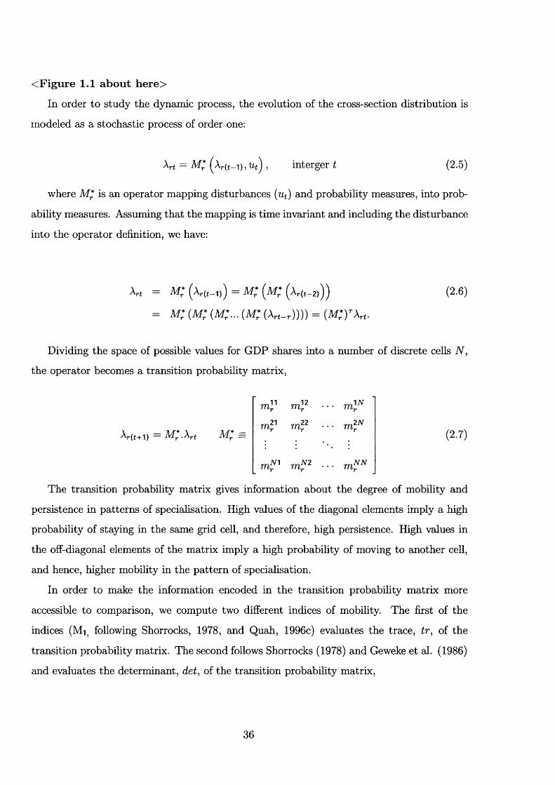
< Figure 1.1 about here>
In order to study the dynamic process, the evolution of the cross-section distribution is
modeled as a stochastic process of order one:
\rt ^ M* Uf) , interger t (2.5)
where M* is an operator mapping disturbances {ut) and probability measures, into prob
ability measures. Assuming that the mapping is time invariant and including the disturbance
into the operator definition, we have:
Art = m ; (a,(,_„) = m ; (m ; (a,(*_2)))
= m ; (m ; (m ;... (m ; (Art_r)))) =
(2 .6)
Dividing the space of possible values for GDP shares into a number of discrete cells N ,
the operator becomes a transition probability matrix.
Ar(( + 1) — M*.Xrt M* =
m.11 m 12 m,IV
m.21 m 22 m:2 N
m:N N
(2.7)
The transition probability matrix gives information about the degree of mobility and
persistence in patterns of speciahsation. High values of the diagonal elements imply a high
probability of staying in the same grid cell, and therefore, high persistence. High values in
the off-diagonal elements of the matrix imply a high probability of moving to another cell,
and hence, higher mobility in the pattern of specialisation.
In order to make the information encoded in the transition probability matrix more
accessible to comparison, we compute two different indices of mobility. The first of the
indices (Mi following Shorrocks, 1978, and Quah, 1996c) evaluates the trace, tr, of the
transition probability matrix. The second follows Shorrocks (1978) and Geweke et al. (1986)
and evaluates the determinant, det, of the transition probability matrix.
36

Ml = M2 = 1 - |det(M ;)| (2.8)
In addition, we also study the ergodic or stationary distribution by taking the limit
T 0 0 The ergodic distribution is the limiting distribution to which the dynamic process
evolves. It gives information about the external shape of the distribution of the GDP shares.
By computation, it is the eigenvector associated with the highest eigenvalue of the transition
probability matrix. Two different scenarios could arise: Figure 2.2 shows the case in which
th e distribution evolves towards a distribution with increasing specialisation, since there is
a bimodal concentration of the values of the GDP shares. In Figure 2.3, we observe higher
concentration of GDP shares in the centre of the distribution over time, and therefore, a
decrease in the degree of specialisation.
< Figures 2.2-2.3 about here>
Finally, using results from Anderson and Goodman (1957), we perform hypothesis testing
on the estimated transition probabilities. The null hypothesis is where refers
to the estimated transition probabilities, and are the probabilities of transition under the
(known) null. The transition probabilities for each state n have an asymptotic distribution
N ( jynl _ Q n l \ 2 T - 1
E I " J r = Y . r ( t ) (2 .9)l= 9 t=o
where 7^ (t) denotes the number of industries in cell n at time t. This test statistic holds
for each state n = 1, ....A". Since the transition probabilities are independently distributed
across states, we may sum over states, and the resulting test statistic is asymptotically
distributed [N {N — 1)).
2.5 D ata Description
The main source of data is the Regio dataset compiled by the European Statistics Office
(Eurostat). We analyse patterns of production across 14 industries in 45 NUTS-1 regions
^^Our analysis here is robust to the arguments presented in Kremer, et al. (2001) about estimation of transition probability matrices and ergodic distributions. We estimate transition probabilities over five-year intervals rather than annual intervals, and compare the ergodic distribution with those implied by the initial distribution.
37

from seven European countries since 1975.^ The choice of countries reflects the availability
of data, and includes Belgium, France, Italy, Luxembourg, Netherlands, Spain, and the
United K i n g d o m . T h i s chapter, therefore, characterises patterns of specialisation across
regions of the seven countries since 1975. As it will be shown below, this is a group of
countries among which there is substantial heterogeneity in patterns of production. The
sample includes several countries close to the “core” of Europe (e.g. Belgium and France)
and others located further towards the “periphery” (e.g. Italy and Spain).
The number and size of NUTS-1 regions varies across European countries. In some
European countries, such as Italy, the NUTS-1 regions correspond to the main regional
political units. In the U.K., they comprise geographical areas such as the North, Southeast,
and Southwest. A full list of NUTS-1 regions in each country is given in Appendix 2.A. We
show below that there is also substantial variation in specialisation across NUTS-1 regions
within a country, for example, from the North of Italy to Sicily.
Patterns of production are analysed at two alternative levels of aggregation. First, we con
sider the three aggregate (one-digit) industries; Agriculture, Manufacturing, and Services.
Second, we exploit more disaggregated information on individual industries within Manufac
turing. These are mainly two-digit industries, and include, for example. Textiles/Clothing
and Chemicals. Again, full details are given in Appendix 2.A.
The Regio dataset provides information on industry value-added and GDP by region,
from which we compute the share of each sector in GDP. The length of the time-series avail
able varies with the level of industrial aggregation. In order to exploit all of the information
available, we consider two samples. First, at the level of the three aggregate industries, we
have an unbalanced panel of approximately 811 observations per industry on the 45 regions
during the period 1975-95 (Sample A). Second, for the disaggregated manufacturing indus
tries, we have an unbalanced panel per industry from approximately 1980 onwards (Sample
B). Full details of the composition of each sample are given in Appendix 2.A.
^^NUTS stands for Nomenclature of Statistical Territorial Units. NUTS-1 regions are the first-tier of subnational geographical units for which Eurostat collects data on the E.U. member countries. See Appendix2. A for more details concerning the data used.
^^Data for other European countries are very incomplete. Where information is available, it is for a very short time period. Data constraints are not such an issue when estimating the neoclassical model in Chapter3. However, it becomes more relevant when introducing issues of economic geography in the analysis (as in Chapter 4). We incorporate additional information from the rest of Europe which is available at the aggregate (regional) level in the econometric estimation of Chapter 4.
38

Table 2.1 presents information on the share of the 3 aggregate industries in each region’s
GDP in 1975, 1985, and 1995. We find substantial variation in patterns of production across
regions at any one point in time, even at the level of the 3 aggregate industries. For example,
the share of Agriculture in GDP in 1985 varies from 0.03 percent in Bel (Brussels) to 11.86
percent in Esp4 (Centre), while the share of Services in GDP in 1985 varies from 81.61
percent in Bel (Brussels) to 49.57 percent in Esp2 (North East). There are also marked
changes in patterns of specialisation over time. The share of Agriculture in GDP in Esp4
(Centre) falls from 14.72 percent in 1980 to 5.39 percent in 1995, while the share of Services
in GDP in Pra3 (Nord-Pas-de-Calais) rises from 46.68 percent in 1975 to 67.00 percent in
1995.
< Table 2.1 about here>
Table 2.2 displays the evolution of the shares of the disaggregated manufacturing indus
tries in GDP. For brevity, only the data for France and Spain are reported. Again, we observe
substantial variation in patterns of production across regions at any one point in time. This
is true both within and between countries. For example, the share of Metal Products and
Machinery (Machine) in GDP in Fra7 (Centre-East) in 1985 is almost three times larger
than that in Fra8 (Mediterranean) and almost six times larger than that in Esp6 (South).
There are also changes in production patterns over time. The share of Chemicals in GDP in
Esp6 (South) falls by 45 percent between 1980 and 1994, while the share of Paper in Fra3
(Nord-Pas-de-Calais) rises by 24 percent over the same period.
< Table 2.2 about here>
2.6 Localisation and Specialisation in Europe: Some
Summary Statistics
We analyse first localisation in Europe by studying the distribution of GDP shares across
countries/ regions for each industry. The analysis is done at two levels; for the sectoral level
(Agriculture, Manufacturing, and Services) and for eleven manufacturing industries. Then,
the pattern of specialisation of countries/ regions is considered by analyzing the distribution
of the GDP shares across industries for each of the geographical unit. In both cases, we do
so by computing a number of summary statistics used in the literature. We first examine the
39

variation in GDP shares across regions for each industry. The higher the variation is, the
more the industry would differ in its location distribution, and the more localised it will be.
We then explore the similarity in specialisation of geographical units by computing pairwise
correlations of GDP shares across all manufacturing industries at different points in time.
An increase in the correlation over time would imply that countries/ regions are becoming
more similar to one another in their production structure. We also evaluate differences in
production structures by computing the Krugman indices across countries/regions. The
index compares the specialisation of a country/region to a defined benchmark. An increase
in the index would imply that countries/ regions are becoming more specialised.
2 .6 .1 In d u stry L oca lisa tion in E u rop e
We analyse the variation in GDP shares for a particular industry across countries, across re
gions, and across regions within a country. Specialisation would be reflected in high variation.
An increase in variation over time would imply that regions or countries are becoming more
dissimilar in their production mix. Countries and regions would then be more vulnerable to
the occurrence of asymmetric shocks.
We compute the coefficient of variation for four different years (1980, 1985, 1990, and
1995) across countries, across all regions, and across regions within a country. The coefficient
of variation is a measure of dispersion, where the standard variation is normalised by the
mean to take account for different means of the GDP shares by industry. We also compute
the relative coefficient of variation, defined as the ratio of the coefficient of variation for
an individual industry to its average value across sectors/ industries at a point in time.
The relative coefficient of variation yields information about the degree of dispersion in an
industry across the different geographical units relative to the average dispersion across all
industries.
Industries are more localised at the regional level. The coefficient of variation reports
higher dispersion at the regional level than at the country level (Table 2.3). At the sectoral
level, manufacturing is becoming more localised (higher variation) while Agriculture and
Services show decreasing variation both at the country and regional levels. Variation in
this part of the analysis, we drop the United Kingdom from our sample and begin in 1980 so that we have a balanced panel of observations across regions and over time. We do not report tables for the relative coefficient of variation for brevity.
40

manufacturing is increasing in all regions within each country, except for the Dutch regions.
Production structures across regions in a country are becoming more distinct.
< Table 2.3 about here>
W ithin the manufacturing industries, industries are more localised at the regional level
(Tables 2.4-2.6). The coefficient of variation is higher at the regional level than at the coun
try level for each of the manufacturing industries. Within countries, we observe differences
across industries. In the categories of Machine and Other, the industry is more localised
across regions within a country than across countries. For other industries, variation differs
depending on the country and the industry considered. There are also marked differences in
localisation when considering regions within a country. For example. Food is more localised
across regions in France than across countries; while it is less localised across Spanish, Dutch
or Belgian regions. Over time, industries show different paths in the evolution of dispersion.
The Transport industry shows increasing localisation at the country and regional levels in
general, but it is becoming less localised in regions within Belgium, Italy, and the Nether
lands.
< Table 2.4-2.6 about here>
The analysis of the relative coefficient of variation yields similar conclusions. Industries
are more localised at the regional level than at the country level, with marked differences
in localisation across regions within a country. Manufacturing is becoming more localised,
although at a slow pace. Services is the least concentrated sector relative to the overall
dispersion across industries, and its variation is decreasing over time. Across manufacturing
industries. Fuel, Metal, Transports, and Textile are the more localised industries both at the
country and regional levels.
2.6 .2 S p ecia lisa tion across E urope
In this section, we analyse the similarities of the pattern of specialisation in manufacturing
industries across countries and regions in Europe, by computing first the correlation of the
whole cross-section distribution of shares across two countries/ regions at a point in time.
Then, we compute the Krugman index, that compares the pattern of specialisation of a
country/region with respect to a benchmark. Our results show evidence of higher diversity
in specialisation at the regional level, as the correlations across regions are lower than across
41
countries. The Krugman indices indicate increasing specialisation over time in manufacturing
industries.
Correlations in the Patterns of Specialisation
We examine pairwise correlations of the GDP shares across the manufacturing industries
among countries/ regions. At the country level, Belgium, Spain, France and Italy have be
come more dissimilar pairwise over time, while Luxembourg, Netherlands and the U.K.
report increasing correlation (Table 2.7). Luxembourg displays a pattern of specialisation
in the manufacturing industries that is extremely diverse with respect to the rest of the
European countries, although becoming more similar over time to the rest of the countries.
Despite Belgium and Spain being the most similar countries in 1980 and in 1995, countries
have changed their degree of similarity over time. '^
< Table 2.7 about here>
At the regional level. Tables 2.8A-F display the correlation of the pattern of specialisation
at the regional level within each country, and that of each region with its country’s patterns
of specialisation. The correlations indicate higher heterogeneity in the degree of similarity in
specialisation. Within a country, pairwise correlations across regions differ significantly. For
example, in Italy, the correlation between regions ital (Northwest) and it2 (Lombardia) is
0.86 in 1980 while between regions itl (Northwest) and ita (Sicily) it is only 0.16, pointing
to substantial north-south differences in specialisation. Over time, there are also significant
changes in the degree of correlation. In Belgium, correlations in 1995 are all lower than
in 1980, indicating that regions are somewhat diverging in their specialisation pattern. In
Spain, we can however observe that all regions have increased their correlation coefficients,
specifically after its EU membership (1986). For instance, the correlation doubled between
regions espl (Northwest) and esp5 (East) in the period 1985-90. In other countries, the
evolution of the correlation is not so homogenous across regions. In France, the correlation
'^The high correlation between Belgium and Spain in their manufacturing structures is contradictory with other results in the literature. However, similar results were found when we sequentially excluded each industry from the sample and when we considered different years to the ones reported here. Further analysis leads to the following conclusions: (i) that the countries have very similar average GDP share for the manufacturing sector as a whole, over the sample period (0.32 for Belgium and 0.35 for Spain), (ii) that the countries display very similar pattern of specialisation across the two-digit industries, (iii) that the GDP shares of Fuel (FP), Chemicals (CHE), Transport (TRP), and Building (BUI) do not display significant correlation over time, while the rest of the industries display very high and significant correlation, (iv) that the evolution of the GDP shares at the two-digit industries is very similar at the country and regional levels.
42

between frai (Ile-de-France) and fraS (Mediterranean) has been increasing during the sample
period as the result of a transition away from industrialisation and towards Services. These
regions report significant increases in Services over the sample period, and they are the
most specialised regions in Services in France. Regions fraS (North-Pas-de-Calais) and fra f
(East) display decreasing correlations: fra3 is becoming less specialised (a more flat profile
of GDP shares in manufacturing industries), while fra f is more specialised in Machine and
Transports. The country showing the largest cross-region differences is Italy. R3 (Northeast)
is the region with a production structure most similar to other Italian regions, while it5
(Centre) is a very distinct region, sharing significant similarities only with one other region
{itl, Northwest).
Correlations in specialisation between a country and its regions are very high for most
of the regions (ranging from 60 to 98 percent when statistically significant). However, we
observe substantial differences in their evolution over time. In France, for example, fra3 cor
relation with the country’s pattern drops from 84 percent to 67 percent, while fraS increases
it from 75 percent to 82 percent. Only 7 out of 45 regions show statistically significant
differences in the pattern of specialisation: esp2 (Northeast) in Spain (1980), ita (Sicily)
and itb (Sardinia) in Italy in all years, ndlf (South) in Netherlands (1980, 1985), and ukb
(Northern Ireland) in 1980, and ukf (East Anglia), uk6 (Southwest), uk7 (West Midlands),
and ukb (Northern Ireland) in 1985.
< Table 2.8A -F about here>
Finally, given that Spain and Belgium were found to be the countries with the most
similar industrial structures. Table 2.9 displays the correlation matrices of the pattern of
specialisation for the Belgian and Spanish regions. We investigate now whether that simi
larity translates into high correlations across all regions in those countries, or whether it is
only due to high correlation between some regions in those c o u n t r i e s . W e observe lower
correlations as regions are more diverse in their production structure. Over time, regions
evolve in different ways: esp7 (Canary Islands) evolves more unlike Belgian regions while
esp2 (Northeast) becomes more similar to Belgian regions over the sample period.
< Table 2.9 about here>
15 We do not report other correlation matrices across other different regions for reasons of brevity.
43

K rugm an Specialisation Indices
In the section above, we analysed pairwise similarities in the pattern of specialisation across
countries and regions within a country. Here, we compare the industrial structure of a
country/region relative to a defined benchmark that exploits information from the whole
sample. For each country/region, the benchmark is defined as the average GDP share
in industry j in the rest of the s a m p l e . F o r each country/region, denote 8jt the share
of the same sector or industry in the production of the rest of the sample at the coun
try/regional levels respectively. We then measure the difference between the industrial struc
ture of country/region i and all other countries/ regions in our sample by taking the absolute
values of the difference between our measure of specialisation {sijt) and summed over all
sectors or industries. Formally, the Krugman index is defined as follows:
K i t = { s i j t — 8 j t ) (2 . 10)j
where i refers to country/region, and j is the industry index.
The Krugman index takes any value between zero and two. If zero, the count ry/region
has an industrial structure that is identical to that of the benchmark, i.e., the rest of the
countries/ regions. If it takes the value of two, the country/region has no industries in
common with the rest of the E.U. Given the level of industry aggregation in the sample, this
is not going to be the case in our sample since all regions and countries produce in all the
sectors and industries specified.
Table 2.10 displays five-year averages of Krugman indices computed for the three sectors
at the country, regional, and within-country levels. The Krugman indices take values close
to zero at this level of aggregation, indicating that countries and regions in Europe are not
really specialised. Krugman indices, however, usually double in value when computed at
the regional level, supporting our previous conclusion that regions are more specialised than
countries. Over time, we observe a decrease in the Krugman indices across countries, across
regions, and across regions within a country. Countries and regions are becoming more
similar over time to the average, in line with our previous results of increasing correlations
this part of the analysis, we again drop United Kingdom from our sample and start in 1980 so that we have a balanced panel of observations across regions and over time. This makes the indices comparable over time.
44

over time. The secular trend of countries and regions decreasing their share of Agriculture
and Manufacturing, while increasing specialisation in Services may underlie these results.
< Table 2.10 about here>
Table 2.11 reports the results for the disaggregated manufacturing industries. At this
more disaggregated level, we observe more variation. At the country level, we find an increase
in specialisation over the sample period in line with Amiti (1999) and Midelfart-Knarvik et
al. (2000a). Luxembourg is the only country reporting a decrease in specialisation, although
it is the most specialised country in the sample. At the regional level, we also find increasing
specialisation, although evolving at a slow pace. Over the entire sample, Krugman indices
display only a 5 percent growth for regions, although higher than at the country level (3
percent).
< Table 2.11 about here>
2.7 Changes in Specialisation at the Country Level: A
Decom position
In the next step, we investigate the nature of changes in the evolution of the pattern of
specialisation at the country level. We discern whether the country-level changes in GDP
shares are mainly due to changes in the GDP shares at the regional level (within-region)
or to changes in the regional shares of GDP (hetween-region). In the first case, changes
in specialisation at the country level will be related to regional changes in specialisation.
Regions will be changing their pattern of specialisation in line with some of the trade the
ories mentioned in the first section. Regions would take advantage of either comparative
advantage, economies of scale, or commercial finkages. In the second case, changes in the
country’s pattern of specialisation would be due to changes in the relative importance of the
region in its country. Ghanges in the latter could possibly be due to, for example, mobility of
factors or region-specific productivity growth. In this regard, comparative advantage would
typically lead over time to between region reallocations of industrial activity, if factors of
production are mobile. If the analysis indicates that changes in specialisation at the country
level are related to within-region changes, then the analysis of specialisation at the regional
is, in itself, meaningful. Otherwise, the analysis will indicate that the interest would need
45

to shift to the relative importance of regions within a country, and the underlinning forces
directing changes in the relative relevance of regions.
Using our measure of specialisation, and performing simple computations, we can express
the country’s GDP share of industry j as a weighted sum of the regional GDP shares of
industry j:
^cjt — ^2 ^rt)rEc
where Scjt is the country’s GDP share of industry j; Srjt is the regional GDP share of industry
j in region r; and uJrt is the ratio of region r ’s GDP to its country’s total GDP. Considering
differences in the expression over time, we arrive at the following expression:
^ ^ c j t ^ "P ^ X ^ r j t ^ ^ r t ) (2.11)rEc rEc
where the first term of the sununation is the within-region effect and the second term is the
between-region effect. Equation 2.11 expresses changes in GDP shares at the country level
as the sum of changes in GDP shares at the regional level (within-region) and changes in
the relative importance of each region in the country (between-region). As an accounting
decomposition, the analysis does not in itself yield to any conclusions regarding causality or
economic determinants for specialisation at the country level.
Table 2.12 reports annualised averages of the total, the within-region, and the between-
region changes in GDP shares for the one-digit sectors. Total changes confirm that all
countries are reducing specialisation in Agriculture and Manufacturing while increasing spe
cialisation in Services. This is as expected due to the secular decline in Agriculture and
Manufacturing in Europe over the sample period. European countries are decreasing their
Manufacturing shares between 0.3 and 0.6 percent every year, while increasing their shares
in Services at an average rate of around 0.5 percent per year. Within-region changes are
driving the changes in the pattern of specialisation at the country level. The magnitude of
the country’s changes are usually smaller than that of within-region changes. Between-region
changes are very small and generally of the opposite direction.
< Table 2.12 about here>
Changes in GDP shares within manufacturing at the country level are also mainly due
46

to changes in GDP shares at the regional level. Tables 2.13-2.14 report the decomposition
for the each of the disaggregated manufacturing industries, with the percentage contribution
of the within- and between-region changes. The Netherlands, for instance, has reduced its
Electronics share in total GDP by 0.07 percent every year, of which 113 percent would
be explained by changes in GDP shares at the regional level, and minus 13 percent by the
relative weight of the regions in total output. However, in contrast to the results for aggregate
industries, some of the between-region changes are of the same direction as the within-region
change. For example, in Ghemicals, the United Kingdom is decreasing its share by 0.01
percent every year, of which 75 percent can be explained by changes in specialisation at the
regional level, and 25 percent by changes in the regional shares of GDP.
< Tables 2.13-2.14 about here>
These results show that within-region changes in specialisation are more important in
accounting for changes in specialisation at the country level than changes in the shares
of regions in a country’s overall economic activity. Regions are changing their pattern of
specialisation more than countries, as the within-region change is typically higher in value
than the total change. Ghanges in regional shares of GDP do play a small role in explaining
changes in specialisation at the country level.
2.8 Dynamics o f Patterns o f Specialisation
In the sections above, we condensed information about specialisation in a number of sum
mary statistics (coefficient of variation, correlations, Krugman indices), and we accounted
for changes in specialisation at the country level. In this section, we explore how the en
tire pattern of specialisation evolves over time. We analyse specialisation dynamics across
manufacturing industries over time, addressing issues related to intra-distribution dynamics
(mobility and persistence) as well as to the evolution of the external shape of the distribu
tion of GDP s h a r e s . B y computing transition probability matrices, we are able to compare
the external shape of the distribution for countries/ regions. We also study whether regions
display higher (lower) mobility in specialisation.
For each geographical unit, we divide the space of possible values of GDP shares into
do not undertake the analysis for the aggregate industries (Agriculture, Manufacturing, and Services) because of the high level of aggregation and small number of observations involved.
47

five discrete cells and estimate the transition probability matrix over five-year periods. The
upper-point of each cell is computed such that industry-year observations are divided roughly
equally between the cells. Each cell corresponds to approximately one quintile of the distri
bution of GDP shares across industries and time.
Tables 2.15-2.20 report the estimated transition probability matrix for each country and
their corresponding r e g i o n s . T h e interpretation of the transition probability matrix goes as
follows. The first column describes the number of industry-time observations placed in each
cell across all time periods. The first numerical row describes the upper-point of each grid
cell. Thereafter, each row describes the probability of passing from one state into another.
Estimated probabilities in the diagonal give information about the degree of persistence in
the pattern of specialisation. Off-diagonal elements inform about the probability of passing to
another state and, therefore, about mobility. The final two rows give the initial distribution
of industry-time observations across grid cells and the ergodic distribution implied by the
estimated transition probability matrix.
< Tables 2.15-2.20 about here>
We find evidence of substantial mobility in patterns of specialisation at the country and
regional levels, suggesting that there are interesting changes in patterns of specialisation in
Europe. In general, the estimated probability of moving out of a quintile of the distribution
after a five-year period ranges from 0.04 to 0.65 at the country level. At the regional level,
the same probabihty increases from 0.04 to 0.79. In general, regions display higher mobility
in their patterns of specialisation, although differences can be found depending on the regions
and countries considered. Mobility is higher in the middle quintiles, with higher persistence
in the extreme quintiles. Comparing the initial and the ergodic distribution, there is a
general pattern of polarisation towards the three lowest quintiles of the distribution at the
country and regional levels. This may reflect two different issues: First, the general decline
in the size of manufacturing industries in Europe over the sample period, and second, the
relative changes in the position of industries with respect to each other, due to different rates
of growth and decline— resulting in changes in the relative position within the distribution
of GDP shares.
^^The entire estimation is undertaken using Professor Danny Quah’s TSRF econometrics package, which is available at http://econ.lse.ac.uk/stajj/dquah/tsrf/html. Responsibility for any results and errors is the author’s alone.
48

In order to ensure that the mobility found in the patterns of specialisation is not due
just to the general decline of manufacturing, we undertake the following robustness test. We
compute the relative GDP share in an individual industry at time t [rsijt) by normalising
the GDP share by the average share of all manufacturing industries in the country/region’s
GDP at time t. The normalisation completely removes the country/region specific decline
in the average GDP shares of manufacturing industries. The analysis now captures spe
cialisation within manufacturing. Transition probability matrices are then estimated with
the relative GDP shares. The estimated transition probabilities capture the changes in the
relative position of industries within the distribution of GDP shares. Table 2.21 reports
the estimation results at the country l e v e l . W e find evidence of mobility of the relative
position of industries within the distribution. The probability of moving out of a quintile of
the distribution ranges from 0.04 to 0.62 (in line with those reported for the GDP shares).
< Table 2.21 about here>
Having concluded that the mobility in the patterns of specialisation is due to the changes
in the relative size of individual industries in Manufacturing, we proceed now to compare
country and regional patterns of specialisation using the GDP shares (sijt). Regions do not
always display higher mobility/persistence in the pattern of specialisation. For instance,
while all Belgian and French regions display higher mobihty with respect to the pattern
of specialisation than the country, Dutch regions display lower mobility. For Belgium, the
average probability of moving out of a quintile of the distribution is 0.19 while for the regions
it ranges from 0.29 to 0.33. For France, the average probability of moving out of a quintile
of the distribution is 0.21, while for the regions it ranges from 0.22 to 0.47. On average,
the probability of moving out of a quintile of the distribution is 0.40 for Netherlands while
it varies from 0.19 to 0.35 at the regional level. In Spain, most of the regions display lower
mobility in their pattern of specialisation than the country.
Mobility indices yield similar conclusions. Table 2.22 uses indices of mobility at the
regional level relative to the corresponding country level, to evaluate the overall degree of
mobility in patterns of specialisation at the regional level. A value above one implies that the
region displays higher mobility than the country. Overall, regions display higher mobility:
in 27 out of the 45 regions, relative mobility indices were higher than one.
Similar results were reported at the regional level, but they are not shown here for reasons of brevity. Results are available in an appendix upon request from the author.
49

< Table 2.22 about here>
Analysing the ergodic distribution, we can study the external shape which the distribution
is evolving to. There is no evidence of the emergence of a bimodal distribution. A comparison
of the initial and ergodic distributions provides evidence of the general decline in the size of
the manufacturing industries during the sample period. The trend is towards a decrease in
mass in the upper quartiles and an increase in mass in the lower quintiles, with evidence of
polarisation of GDP shares towards the bottom quintiles of the distribution. Exceptions are
Luxembourg and ital, which report an increase in mass in the upper quintiles.
There are cases of complete polarisation. For example, at the country level, Belgium
displays an ergodic distribution leading to complete polarisation to the lower quintile of
the distribution. In Spain, the results indicate complete polarisation for four of the regions
{espl, esp3, esp4, and esp6). Furthermore, there are significant differences between coun
try and regional data. For example, Italy’s ergodic distribution is characterised by partial
polarisation towards the lower quintiles of the distribution. At the regional level, however,
regions show a very diverse pattern of specialisation. While ital reports polarisation towards
the upper quintiles of the distribution, ita7 evolves towards convergence on the degree of
specialisation for the industries under consideration (most of the mass is concentrating in
the central quintiles of the distribution), and itaa, and itab evolve towards complete po
larisation (all the distribution concentrates in the lowest quintile). Finally, there are cases,
although exceptional, in which two ergodic distribution were reported (/ra7, it6), signalling
that the dynamic process is not fully determined. Given the regional differences regarding
intra-distribution dynamics and the ergodic distribution, the results seem to suggest that
analysing specialisation dynamics at the regional level can bring further insights about how
specialisation evolves over time.
Next, we explore the cross-country and within-country differences in the dynamic process.
Table 2.23 examines the statistical significance of the cross-country differences. The null
hypothesis is that the Data Generating Process (DGF) is equal to the transition probability
matrix that was estimated for France. France is the largest country in our sample, and by
location, it is at the core of our sample. We test whether the estimated transition probability
matrix for each of the other countries is statistically significantly different from this known
null. The null hypothesis is rejected at the 1 percent level for Belgium, Luxembourg and
Netherlands (the small countries), but it is not rejected for Italy, Spain and United Kingdom.
50

Results are somehow surprising as we might expect that Belgium and Netherlands display
a similar dynamic process according to which the industrial structures evolves to that of
France, as they are commonly thought as being at the core of Europe and distinct from the
periphery.
< Table 2.23 about here>
Table 2.24 reports the statistics on the within-country differences with respect to the
dynamic process. The null hypothesis is that a region’s Data Generating Process (DGF)
equals the transition probability matrix estimated for the corresponding country. Overall, we
find evidence of within-country differences in the evolution of the patterns of specialisation.
We are unable to reject the null hypothesis in only 14 out of 45 regions. However, conclusions
differ depending on the country considered. In Belgium and Italy, none of the regions show
statistically significant differences in the evolution of the patterns of specialisation to the
null hypothesis. For France, Spain and United Kingdom, most of the regions rejected the
null hypothesis, reflecting statistically significant differences in the evolution of the patterns
of specialisation at the regional level.
These results suggest that specialisation dynamics at the regional level should be taken
into account in addition to specialisation dynamics at the country level. Regions show
more mobility in the degree of specialisation and significant differences to countries in the
dynamic process. These results complement the analysis of the patterns of specialisation
across manufacturing industries presented above, regarding the evolution of the pairwise
correlation. The summary statistics analysis relate to the external shape rather than to the
intra-distribution dynamics, and therefore, some information is lost from not considering the
evolution of the entire distribution. The estimation of the transition probability matrices
gives additional insights about the dynamic process. Substantial within-country differences
are revealed through the transition probability matrices, that we were unable to uncover
with the use of summary statistics.
< Table 2.24 about here>
Finally, we perform a series of independent robustness tests. The analysis above made
a series of assumptions, all of them testable by using eq.2.9. We have assumed that the
operator M* was time invariant. We test this assumption as well as whether there exist
significant differences when we consider other lengths of the transition period or a different
number of grid cells.
51

Our results are robust to each of these tests. First, in the estimation above, we assume
the stationarity of the dynamic process for the estimation of the transition probability ma
trices. We then test for this assumption by eliminating the last five years of each sample,
and reestimating the transition probability matrices. We test for the null hypothesis that
the data generating processes are the same under the two samples. The null hypothesis can
not be rejected for any country or region except for Bel (Brussels). Second, when estimat
ing transition probabilities matrices, boundaries between grid cells were chosen such that
observations were allocated roughly equally across cells. We are therefore always concerned
with movements of industries between quintiles of the GDP shares distribution. Now, we
consider the space of GDP share values to be divided in four grid cells instead of five and
transition probability matrices were reestimated over five-year periods. We again find evi
dence of mobility in the patterns of specialisation at the country and regional levels, with
similar mobility indices reported. Finally, we estimate the transition probability matrices
by choosing three-year transitions instead of five-year transitions. The estimated transition
probability matrices yield very similar results at the country and regional levels.
2.9 Conclusions
This chapter has analysed the evolution of specialisation in European countries and regions,
combining the rich variation existing at the country and regional levels over the period 1975-
95. We use a theory-consistent measure of specialisation, the GDP share of an industry at
a point in time, which is derived from the neoclassical theory of trade. The analysis concen
trates on uncovering the key facts concerning the evolution of patterns of specialisation in
European countries. Subsequent chapters analyse the econometric determinants of evolving
patterns of specialisation at the regional level.
The analysis above suggests the following conclusions. In the first part of the analysis,
we use summary statistics to study the patterns of specialisation at the country and regional
levels. Regional GDP shares vary markedly. Variation is higher across regions than across
countries, indicating that regions are more specialised than countries. There are notable
changes over time, and regions within countries show different patterns in the evolution of
variation over time. Pairwise correlations indicate that, in general, countries’ patterns of
specialisation are becoming more dissimilar over time. When comparing a region’s pattern
52

of specialisation with that of its country, we find high heterogeneity in the degree of similarity
in specialisation. When analysing specialisation relative to Europe, countries and regions
also show increasing specialisation in the manufacturing industries, although at a slow pace.
When studying the nature of the changes in specialisation at the country level, an account
ing decomposition indicates that changes in specialisation at the country level are mainly
due to changes in specialisation at the regional level. There is no evidence of significant
between-region changes in terms of shares of a coimtry’s GDP, and the relative importance
of regions seem to remain fairly constant over the sample period.
Because the summary statistics condensed information about specialisation, we also ex
plore how the entire pattern of specialisation evolves over time. We analyse specialisa
tion dynamics across manufacturing industries over time, addressing issues related to intra
distribution dynamics (mobility and persistence) as well as to the evolution of the external
shape of the distribution of GDP shares. By computing transition probability matrices, we
are able to compare the external shape of the distribution for countries/regions. We also
study whether regions display higher (lower) mobility in specialisation. The analysis of the
evolution of the entire distribution of GDP shares reveals that no evidence of an increase in
the overall degree of specialisation over time, but of significant mobility. The sample period
is characterised by a decline in the average share of manufacturing in GDP. This is reflected
in a polarisation of the distribution of GDP shares towards the bottom two quintiles of
the distribution for most of the countries and regions under analysis. We find evidence of
substantial mobility in patterns of specialisation at the country and regional levels. This
mobility suggests that there are significant changes in the patterns of specialisation. In gen
eral, regions display higher mobility in their patterns of specialisation, although differences
can be found depending on the regions and countries considered. Also, there is evidence of
higher mobility in the middle quintiles and higher persistence in the extreme quintiles at the
regional level. Comparing the initial and the ergodic distribution, there is a general pattern
of polarisation toward the three lowest quintiles of the distribution at the country and re
gional levels. We find evidence of within-country differences in the evolution of the patterns
of specialisation: 31 out of 45 of the regions follow a dynamic process that is statistically
significantly different to that of their country.
Having found significant variation in specialisation at the regional level, the two following
chapters will investigate the role of factor endowments and economic geography in explain
53

ing the variation in the patterns of specialisation at the regional level in Europe. Chapter 3
analyses the role of factor endowments. Although factor endowments explain a sizable pro
portion of the variation in patterns of specialisation, there remains substantial unexplained
variation, especially for the disaggregated industries within manufacturing, suggesting a role
for other considerations such as those emphasised in the new economic geography literature.
Chapter 4 of this thesis extends further the analysis of the determinants of specialisation by
incorporating considerations of economic geography alongside those of factor endowments
and factor intensities to explain the pattern of specialisation within manufacturing industries
in European regions.
54

Table 2.1: Shares of Agriculture, Manufacturing, and Services in GDP (percent)
Region Year Agric Manuf Serv Region Year Agric Manuf ServBel 1975 0.01 28.58 71.42 Pra7 1975 4.30 46.46 49.24
1985 0.03 18.35 81.61 1985 3.11 36.85 60.041995 0.02 15.75 1995 2.43 32.17 65.40
Be2 1975 3.64 42.45 53.92 Pra8 1975 5.98 32.96 61.061985 2.64 37.39 59.96 1985 4.27 25.21 70.521995 1.52 34.27 64.21 1995 3.24 20.26 76.51
Be3 1975 3.91 39.93 56.16 Itl 1975 4.46 48.20 47.341985 3.00 32.24 64.76 1985 3.12 41.17 55.711995 1.76 27.36 70.88 1995 2.42 36.87 60.71
Espl 1980 9.35 39.22 51.43 It2 1975 2.87 55.18 41.951985 8.07 39.29 52.64 1985 2.05 45.49 52.451995 4.82 34.45 60.73 1995 1.56 41.21 57.23
Esp2 1980 5.93 48.12 45.95 It3 1975 6.03 45.82 48.151985 4.59 45.84 49.57 1985 4.38 40.96 54.661995 2.25 42.12 55.63 1995 3.13 36.71 60.17
Esp3 1980 0.55 30.58 68.86 It4 1975 8.72 47.13 44.151985 0.32 28.61 71.08 1985 5.75 40.87 53.381995 0.17 25.26 74.57 1995 3.70 36.94 59.36
Esp4 1980 14.72 34.61 50.67 It5 1975 5.32 45.34 49.341985 11.86 36.10 52.04 1985 3.36 41.09 55.551995 5.39 34.50 60.11 1995 2.64 34.62 62.75
Esp5 1980 4.24 42.19 53.56 It6 1975 4.40 26.02 69.571985 3.00 39.44 57.56 1985 2.59 25.09 72.321995 1.57 34.55 63.87 1995 1.62 21.24 77.14
Esp6 1980 10.91 33.13 55.97 It7 1975 10.70 39.19 50.111985 10.84 29.25 59.91 1985 6.72 34.32 58.951995 6.15 27.91 65.95 1995 4.53 32.04 63.43
Esp7 1980 8.25 21.38 70.37 Xt8 1975 10.26 31.29 58.451985 4.80 18.41 76.79 1985 5.38 27.71 66.911995 2.06 18.56 79.38 1995 3.33 24.30 72.36
Pral 1975 0.68 34.87 64.45 It9 1975 14.17 31.02 54.811985 0.40 29.50 70.10 1985 9.42 27.81 62.771995 0.18 22.54 77.28 1995 6.49 24.49 69.02
Era2 1975 8J3 43.58 47.69 Ita 1975 12.56 29.54 57.901985 7.41 36.07 56.52 1985 9.36 28.33 62.321995 4.27 32.69 63.04 1995 5.73 21.47 72.80
Fra3 1975 4.04 49.28 46.68 Itab 1975 9.09 36.40 54.511985 2.62 35.80 61.58 1985 5.96 33.64 60.391995 1.35 31.66 67.00 1995 4.11 27.37 68.52
Fra4 1975 4.45 47.50 48.05 Lux 1975 3.24 39.18 57.571985 3.71 37.48 58.81 1985 2.36 34.04 63.601995 2.60 34.66 62.74 1995 1.21 31.61 67.19
Pra5 1975 11.38 37.48 51.14 Nidi 1975 7.55 36.91 55.541985 7.98 29.24 62.78 1985 4.33 35.08 60.581995 5.24 27.08 67.69 1995 4.45 38.53 57.02
Pra6 1975 8.57 37.15 54.28 Nld2 1975 7.24 35.21 57.551985 6.67 30.56 62.77 1985 6.12 29.77 64.111995 4.41 24.37 71.22 1995 4.19 27.24 68.58
55

Table 2.1 (cont): Shares of Agriculture, Manufacturing, and Services in GDP (percent)
Region Year Agric Manuf Serv Region Year Agric Manuf ServNld3 1975 3.73 32.48 63.80 Uk6 1975 3.27 36.86 59.87
1985 3.29 28.23 68.48 1980 3.23 35.60 61.171995 2.71 23.64 73.65 1985 2.16 34.36 63.48
NId4 1975 4.70 43.21 52.09 Uk7 1975 1.51 48.94 49.551985 5.48 37.25 57.27 1980 1.71 46.34 51.941995 3.55 32.62 63.83 1985 1.23 43.64 55.13
Ukl 1975 2.04 50.04 47.93 Uk8 1975 0.87 45.53 53.601980 1.58 47.29 51.12 1980 0.70 45.46 53.841985 1.37 41.37 57.25 1985 0.53 44.32 55.15
Uk2 1975 2.31 46.46 51.23 Uk9 1975 2.81 45.57 51.611980 1.92 44.88 53.21 1980 2 j# 45.14 51.981985 1.43 41.40 57.17 1985 2.48 45.93 51.59
Uk3 1975 2.76 48.36 48.88 Uka 1975 2.98 43.73 53.281980 2.76 46.45 50.79 1980 2.39 42.17 55.441985 1.59 44.29 54.11 1985 1.69 38.82 59.49
Uk4 1975 6.56 36.12 57.32 Ukb 1975 3.40 43.37 53.231980 5.78 35.93 58.29 1980 3.30 37.21 59.491985 3.07 36.02 60.91 1985 2.89 36.00 61.11
Uk5 197519801985
0.820.850.48
32.1432.5129.46
67.0366.6570.06
Notes: Figures may not sum to exactly 100 due to rounding.
56

Table 2.2: Shares of the Disaggregated Manufacturing Industries in GDP in France andSpain (percent)
Region Year Fuel Metal Mineral Chem Machine TranspEspl 1980 7.47 5.61 2.13 1.34 3.49 2.82
1985 9.56 4.98 2.18 1.69 2.901994 7.84 2.63 1.92 0.79 2.34 2.19
Esp2 1980 4.52 5.14 2.12 1.96 12.65 3.011985 5.77 4.29 1.72 1.98 10.15 3.351994 7.00 2.11 1.69 1.10 8^0
Esp3 1980 1.14 0.60 1.21 2.71 7.27 2.541985 2.27 0.24 0.89 2.76 6.00 2.091994 2.41 0.16 0.77 1.75 4j& 1.76
Esp4 1980 6.16 0.41 2.06 1.41 2.30 3.741985 0.33 1.87 1.67 1.97 2.781994 9.50 0.17 1.80 1.10 1.88 2.11
Esp5 1980 3.41 0.61 2.37 3.41 6.09 2.721985 4.83 0.42 2.22 3.47 5.58 2.051994 4.80 0.21 1.86 2.67 4.53 1.75
Esp6 1980 5.69 1.14 2.61 1.39 1.89 1.711985 4.80 1.41 1.38 2.24 1.68 1.451994 6.04 0.61 1.14 0.77 1.34 1.09
Esp7 1980 3.36 0.00 1.08 0.38 0.53 0.181985 4.18 0.01 0.86 0.24 0.63 0.311994 5.12 0.03 0.79 0.13 0.42 0.29
Pral 1980 4.48 0.87 0.64 2.52 7.88 4.471985 5.56 0.70 0.55 2.52 7.11 2.491994 5.06 0.28 0.49 2.01 4.78 1.87
Fra2 1980 3.89 1.42 1.57 2.81 9.96 3.931985 5.47 1.09 1.18 2.26 8.07 2.201994 4.57 0.88 1.14 2.46 7.62 2.68
Fra3 1980 5.47 4.00 2.36 2.80 7.38 3.771985 4.69 2.59 1.99 1.73 5.47 2.351994 3.06 2.55 1.65 2.49 4.41 2.29
Fra4 1980 3.65 3.86 1.77 2.52 9.27 5.481985 3.34 2.41 1.55 1.98 8^8 4.261994 2.71 1.39 1.18 1.65 7.81 5.24
Fra5 1980 3.22 Oj& 1.31 .75 6.34 4.171985 2.85 0.34 0.95 0.73 5.40 2.501994 2.46 0.20 0.95 0.68 5.34 2.57
Pra6 1980 6.99 0.63 1.50 2.36 4.61 2.931985 6.94 0.56 1.09 1.30 4.16 2.331994 3.74 0.21 1.02 1.15 4.05 2.47
Pra7 1980 3.57 1.55 1.29 2.64 12.06 2.961985 4.18 1.09 1.05 2.39 9.83 1.611994 4.02 1.00 .87 2.16 8^G 1.43
FraS 1980 4.41 1.85 1.41 1.90 3jG 1.591985 5.42 1.51 1.14 1.31 3.53 1.281994 4.22 0.86 .89 1.55 2.80 0.99
See Appendix l.A for industry definitions.
57

Table 2.2 (cont): Shares of the Disaggregated Manufacturing Industries in GDP in Franceand Spain (percent)
Food Textile Paper Other ConstrEspl 1980
19851994
4.204^74.53
0.740.880.69
0.540.750.51
1.691.341.08
9.197.539.06
Esp2 1980 5.00 1.55 2.01 4.11 6.051985 5.64 1.64 1.97 3.63 5.701994 4.59 0.95 1.45 2.52 6^a
Esp3 1980 2.67 1.32 1.32 1.66 7.721985 3.08 1.54 2.11 1.57 6.061994 2.09 0.78 2.01 1.04 8.14
Esp4 1980 5.11 1.57 0.58 2.29 8.981985 5.65 1.80 0.74 1.92 7.501994 4.76 1.21 0.52 1.54 9.85
Esp5 1980 4.35 6.49 1.50 3.24 8.011985 4.99 5.54 1.52 2.88 5.941994 3.97 3.39 1.38 2.34 6.94
Esp6 1980 5.94 1.32 0.56 1.07 9.811985 6.65 1.33 0.62 Oj# 6.801994 5.07 0.79 0.46 0.73 8.67
Esp7 1980 4.63 0.09 0.72 0.53 9.891985 3.05 0.31 0.59 0.70 7.531994 3.10 0.17 0.49 0.40 7.36
Fral 1980 2.26 1.08 1.80 1.16 5.611985 1.63 0.95 2.21 1.03 4.731994 1.41 0.70 2.36 0.72 4.04
Pra2 1980 6.08 2.05 1.31 2^2 6.731985 4.68 1.79 1.46 2.51 5.351994 3.59 1.16 1.46 2.62 4.99
Fra3 1980 5.43 5.34 1.46 1.31 6.821985 4.10 4.71 1.67 1.231994 4.23 2.54 1.81 1.48 4.58
Pra4 1980 4.71 2.66 1.49 2.45 6.621985 4.03 2.44 1.67 2.48 5.041994 3.78 1.35 1.76 2.58 4.98
Fra5 1980 6.73 2.25 1.09 2.42 8.711985 4.99 1.94 1.22 2.46 5.851994 5.04 1.19 1.30 2.49 5.34
Pra6 1980 4.09 2.39 1.31 1.85 7.521985 3.27 1.98 1.35 1.64 5.931994 3.35 0.99 1.24 1.76 5.16
Era? 1980 3.60 2.96 1.44 4.00 7.431985 2.94 2.46 1.37 3.69 6.221994 2.69 1.83 1.27 3.27 5.41
FraS 1980 3.70 0.82 0.68 0.92 9.121985 2.36 0.59 0.78 0^& 6.421994 2.17 0.37 0.75 0.83 5.35
(a) See Appendix l.A for industry definitions.
58

Table 2.3: Evolution of the Coefficient of Variation for the One-Digit Sectors, at the Countryand Regional Levels
Years Agriculture Manufacture ServicesAcross Countries 1980 0.427 0.061 0.062
1985 0.338 0.058 0.0471990 0.344 0.063 0.0351995 0.373 0.076 0.036
Across all EU 1980 0.618 0.212 0.145regions 1985 0.596 0.239 0.141
1990 0.575 0.205 0.1111995 0.559 0.224 0.104
Across all regions Bel 1980 0.860 0.261 0.156within a country 1985 0.857 0.336 0.165
1990 0.872 0.321 0.1461995 0.861 0.363 0.139
Esp 1980 0.601 0.243 0.1651985 0.678 0.269 0.1721990 0.667 0.201 0.1271995 0.699 0.249 0.128
Fra 1980 0.550 0.153 0.1161985 0.581 0.139 0.0801990 0.592 0.165 0.0841995 0.567 0.190 0.082
It 1980 0.466 0.219 0.1281985 0.477 0.202 0.1031990 0.383 0.231 0.1101995 0.440 0.232 0.099
Ndl 1980 0.226 0.309 0.2161985 0.261 0.384 0.2641990 0.244 0.222 0.2221995 0.208 0.213 0.108
Note: The table reports the coefficient of variation, a measure of dispersion, computed as the standard variation at the industry level normalised by the mean.
59
Table 2.4: Evolution of the Coefficient of Variation for the Manufacturing Industries, at theCountry and Regional Levels
Years Fuel Metal Mineral Chem MachineAcross Countries 1980 0.559 1.389 0.313 0.344 0.341
1985 0.631 1.421 0.299 0.408 0.2861990 0.386 1.276 0.474 0.470 0.2011995 0.350 0.902 0.509 0.525 0.223
Across all EU 1980 1.134 1.362 0.501 0.452 0.579regions 1985 1.052 1.440 0.468 0.510 0.554
1990 0.812 1.249 0.475 0.538 0.5531995 0.655 1.010 0.512 0.548 0.564
Across all regions Bel 1980 0.144 1.053 0.952 0.507 0.327within a country 1985 0.358 0.992 1.019 0.667 0.283
1990 0.407 0.933 0.891 0.842 0.3121995 0.363 0.977 0.987 0.736 0.341
Esp 1980 0.465 1.272 0.296 0.556 0.8511985 0.478 1.250 0.355 0.501 0.8171990 0.380 1.252 0.348 0.585 0.8431995 0.377 1.303 0.354 0.689 0.849
Fra 1980 0.278 0.764 0.328 0.300 0.3761985 0.278 0.648 0.357 0.352 0.3381990 0.268 0.720 0.356 0.319 0.3411995 0.227 1.014 0.319 0.389 0.390
It 1980 0.506 0.688 0.459 0.486 0.6421985 0.554 0.653 0.437 0.494 0.6141990 0.474 0.649 0.384 0.436 0.6371995 0.471 0.730 0.434 0.492 0.612
Ndl 1980 1.333 0.847 0.518 0.437 0.4901985 1.353 0.604 0.406 0.383 0.4511990 1.222 0.572 0.479 0.323 0.4831995 1.006 0.588 0.524 0.246 0.452
Note: The table reports the coefficient of variation, a measure of dispersion, computed as the standard variation at the industry level normalised by the mean.
60

Table 2.5: (cont) Evolution of the Coefficient of Variation for the Manufacturing Industries,at the Country and Regional Levels
Transp Food Textile Paper Other ConstrAcross Countries 1980 0.603 0.227 0.714 0.274 0.333 0.067
1985 0.544 0.283 0.767 0.274 0.422 0.1481990 0.538 0.250 0.721 0.272 0.417 0.2071995 0.626 0.283 0.805 0.233 0.328 0.338
Across Regions 1980 0.671 0.351 0.940 0.425 0.572 0.2541985 0.635 0.381 0.982 0.461 0.559 0.2771990 0.681 0.381 0.940 0.488 0.568 0.2701995 0.709 0.436 1.029 0.483 0.577 0.299
Across Regions Be 1980 0.668 0.225 0.741 0.232 0.953 0.228within a country 1985 0.304 0.216 0.827 0.115 0.948 0.237
1990 0.346 0.189 0.695 0.181 0.820 0.1901995 0.367 0.291 0.819 0.144 0.877 0.236
Esp 1980 0.480 0.222 1.128 0.604 0.597 0.1611985 0.480 0.278 0.913 0.561 0.577 0.1221990 0.430 0.248 0.924 0.629 0.606 0.1781995 0.529 0.274 0.928 0.613 0.598 0.136
Fra 1980 0.320 0.320 0.566 0.247 0.484 0.1571985 0.369 0.331 0.589 0.281 0.483 0.1061990 0.527 0.345 0.524 0.274 0.450 0.0881995 0.610 0.360 0.555 0.320 0.467 0.103
Italy 1980 0.872 0.337 0.764 0.506 0.571 0.3141985 0.883 0.402 0.828 0.597 0.572 0.2901990 0.864 0.407 0.748 0.633 0.562 0.1941995 0.621 0.397 0.752 0.623 0.547 0.173
Ndl 1980 0.311 0.151 0.814 0.144 0.466 0.1461985 0.353 0.174 0.871 0.105 0.413 0.0601990 0.389 0.316 0.761 0.179 0.242 0.1181995 0.265 0.368 0.761 0.142 0.348 0.116
Note: The table reports the coefficient of variation, a measure of dispersion, computed as the standard variation at the industry level normalised by the mean.
61

Table 2.6: Matrix of Correlation of the Pattern of Specilisation across Countries, Manufacturing Industries
Year=1980 Be Esp Fra It Lux NdlEsp 0.97* 1.00Fra 0.89* 0.90* 1.00It 0.73* 0.78* 0.82* 1.00
Lux 0.27 0.19 0.08 0.11 1.00Ndl 0.86* 0.77* 0.72* 0.44 0.07 1.00UK 0.76* 0.68* 0.77* 0.45 -0.06 0.93*
Year=1985 Be Esp Fra Ita Lux NdlEsp 0.93* 1.00Fra 0.90* 0.87* 1.00It 0.67* 0.68* 0.83* 1.00
Lux 0.09 -0.03 -0.02 -0.02 1.00Ndl 0.78* 0.76* 0.74* 0.36 -0.05 1.00UK 0.84* 0.84* 0.85* 0.49 -0.10 0.97*
Year=1990 Be Esp Fra Ita Lux NdlEsp 0.90* 1.00Fra 0.91* 0.80* 1.00It 0.76* 0.72* 0.86* 1.00
Lux 0.38 0.34 0.27 0.32 1.00Ndl OjW* 0.80* 0.83* 0.59 0.13 1.00
Year=1995 Be Esp Fra Ita Lux NdlEsp 0.91* 1.00Fra Oj#* 0.78* 1.00It 0.68* 0.66* 0.80* 1.00
Lux 0.63* 0.74* 0.54 0.64* 1.00Ndl 0.90* 0.83* 0.83* 0.57 0.48 1.0000
Notes: The table reports the pairwise correlations of the GDP shares across the manufacturing industries between geographical units. Bold figures refer to the highest pairwise correlation in the year under analysis.* refers to the correlation being statistically significant different from zero at the 5 percent significance level.
62

Table 2.7: Correlation Matrices of the Pattern of Specialisation for the Regions within the same Country
Table 2 .8 .A: Belgium
Year =1980 Be Lux Bel Be2Lux 0.27 1.00Bel 0.91* 0.02 1.00Be2 0.97* 0.14 0.88* 1.00Be3 0.89* 0.52 0.71* 0.75*
Year=1985 Be Lux Bel Be2Lux 0.09Bel 0.83* -0.14 1.00Be2 0.96* -0.02 0.75* 1.00Be3 0.81* 0.44 0.61* 0.64*
Year=1990 Be Lux Bel Be2Lux 0.38Bel 0.84* 0.19 1.00Be2 0.96* 0.23 0.77* 1.00Be3 0.81* 0.68* 0.62* 0.65*
Year =1995 Be Lux Bel Be2Lux 0.63*Bel 0.86* 0.59 1.00Be2 0.97* 0.47 0.80* 1.00Be3 0.81* 0.86* 0.65* 0.66*
Notes: The table reports the pairwise correlations of the GDP shares across the manufacturing industries between geographical units. Bold figures refer to the highest pairwise correlation in the year under analysis.* refers to the correlation being statistically significant different from zero at the 5 percent significance level.
63

Table 2.8.B: Netherlands
Year=1980 Ndl Ndll Ndl2 Ndl3Ndll 0.83* 1.00Ndl2 0.73* 0.26 1.00Ndl3 0.88* 0.56 0.77* 1.00Ndl4 0.59 0.12 0.87* 0.68*
Year =1985 Ndl Ndll Ndl2 Ndl3Ndll 0.94* 1.00Ndl2 0.60* 0.33 1.00Ndl3 0.79* 0.59 0.73* 1.00Ndl4 0.37 0.08 0.83* 0.60
Year =1990 Ndl Ndll Ndl2 Ndl3Ndll 0.72* 1.00Ndl2 0.79* 0.18 1.00Ndl3 0.97* 0.69* 0.74* 1.00Ndl4 0.67* 0.04 0.90* 0.59
Year=1995 Ndl Ndll Ndl2 Ndl3Ndll 0.84* 1.00Ndl2 0.80* 0.34 1.00Ndl3 0.97* 0.92* 0.64* 1.00Ndl4 0.64* 0.16 0.93* 0.42
Notes: The table reports the pairwise correlations of the GDP shares across the manufacturing industries between geographical units. Bold figures refer to the highest pairwise correlation in the year under analysis.* refers to the correlation being statistically significant different from zero at the 5 percent significance level.
64
Table 2 .8 .C: Spain
Year =1980 Es Esl Es2 Es3 Es4 Es5 Es6Esl 0.74* 1.00Es2 0.60 0.41 1.00Es3 0.83* 0.39 0.70* 1.00Es4 0.85* 0.79* 0.23 0.52 1.00Es5 & 83* 0.32 0.39 0.74* 0.59 1.00Es6 0.86* 0.83* 0.23 0.51 0.95* 0.58 1.00Es7 0.84* 0.77* 0.20 0.57 0.91* 0.59 0.97*
Year =1985 Es Esl Es2 Es3 Es4 Es5 Es6Esl 0.75* 1.00Es2 0.69* 0.47 1.00Es3 0.76* 0.27 0.71* 1.00Es4 0.86* 0.87* 0.38 0.40 1.00Es5 0.83* 0.32 0.49 0.72* 0.60 1.00Es6 0.87* 0.76* 0.40 0.52 0.84* 0.61* 1.00Es7 0.85* 0.78* 0.35 0.58 0.86* 0.58 0.88*
Year=1990 Es Esl Es2 Es3 Es4 Es5 Es6Esl 0.89* 1.00Es2 0.71* 0.55 1.00Es3 0.88* 0.65* 0.74* 1.00Es4 0.92* 0.94* 0.53 0.65* 1.00Es5 0.92* 0.68* 0.65* 0.85* 0.79* 1.00Es6 0.93* 0.93* 0.46 0.75* 0.91* 0.80* 1.00Es7 0.93* 0.94* 0.46 0.74* 0.94* 0.79* 0.99*
Year=1995 Es Esl Es2 Es3 Es4 Es5 Es6Esl 0.92* 1.00Es2 0.81* 0.72* 1.00Es3 0.88* 0.72* 0.71* 1.00Es4 0.95* 0.96* 0.69* 0.73* 1.00Es5 0.94* 0.75* 0.75* 0.86* 0.83* 1.00Es6 0.96* 0.96* 0.66* 0.78* 0.97* 0.84* 1.00Es7 0.95* 0.96* 0.63* 0.79* 0.97* 0.82* 0.99*
Notes: The table reports the pairwise correlations of the GDP shares across the manufacturing industries between geographical units. Bold figures refer to the highest pairwise correlation in the year under analysis.* refers to the correlation being statistically significant different from zero at the 5 percent significance level.
65
Table 2.8.D: France
Year=1980 Fra Fral Fra2 FraS Fra4 FraS Fra6 Fra7Pral 0.93* 1.00Pra2 0.96* 0.87* 1.00FraS 0.84* 0.72* 0.78* 1.00Fra4 0.93* 0.88* 0.92* 0.81* 1.00Pra5 0.89* 0.71* O^Kf 0.75* 0.78* 1.00Pra6 0.81* 0.73* 0.68* 0.74* 0.58 0.78* 1.00Pra7 0.91* 0.86* 0.93* 0.72* 0.89* . 0.72* 0.58 1.00Fra8 0.7S* 0.60 0.61* 0.69* 0.57 0.79* 0.87* 0.52
Year=1985 Fra Fral Fra2 FraS Fra4 FraS Fra6 Fra7Fral 0.94* 1.00Fra2 0.98* 0.89* 1.00FraS 0.80* 0.66* 0.77* 1.00Fra4 0.87* 0.79* 0.88* 0.70* 1.00Fra5 0.8S* 0.6S* 0.86* 0.74* 0.82* 1.00Fra6 0.86* 0.80* 0.80* 0.76* 0.57 0.73* 1.00Fra7 0.92* 0.8S* 0.92* 0.70* 0.89* 0.79* 0.64* 1.00Fra8 0.84* 0.77* 0.75* 0.72* 0.55 0.70* 0.93* 0.64*
Year=1990 Fra Fral FVa2 FraS Fra4 FraS Fra6 FVa7Fral 0.93* 1.00Fra2 0.97* 0.86* 1.00FraS 0.88* 0.73* 0.84* 1.00Fra4 0.84* 0.70* 0.86* 0.75* 1.00FraS 0.86* 0.64* 0.88* 0.82* 0.78* 1.00Fra6 0.93* 0.85* 0.86* 0.83* 0.72* 0.89* 1.00Fra7 0.94* 0.85* 0.96* 0.83* 0.81* 0.78* 0.78* 1.00Fra8 0.80* 0.76* 0.70* 0.76* 0.45 0.69* 0.88* 0.65*
Yeax=1995 Fra Fral Fra2 FraS Fra4 FraS Fra6 Fra7Fral 0.90* 1.00Fra2 0.98* 0.8S* 1.00FraS 0.67* 0.49 0.62* 1.00Fra4 0.82* 0.62* 0.85* 0.53 1.00FraS 0.8S* 0.59 0.82* 0.67* 0.81* 1.00Fra6 0.92* 0.80* 0.84* 0.65* 0.70* 0.90* 1.00Fra7 0.90* 0.73* 0.93* 0.57 0.76* 0.77* 0.72* 1.00Fra8 0.82* 0.82* 0.72* 0.68* 0.45 0.66* 0.90* 0.61*
Notes: The table reports the pairwise correlations of the GDP shares across the manufacturing industries between geographical units. Bold figures refer to the highest pairwise correlation in the year under analysis.* refers to the correlation being statistically significant different from zero at the 5 percent significance level.
66

Table 2.8.E: Italy
Year=1980 It Itl It2 Its It4 Its Itfi It? Its It9 ItaItl 0.82* 1.00It2 0.89* 0.86* 1.00Its 0.95* o.?o* 0.82* 1.00It4 0.90* 0.?fi* 0.8S* 0.84* 1.00Its O.fiS* 0.S5 0.49 o.?o* 0.46 1.00Itfi 0.85* 0.54 0.64* 0.80* 0.?fi 0.41 1.00It7 0.fi9* O.SO O.Sl 0.64* 0.5? 0.48 0.8?* 1.00Its 0.92* 0.69* O.fi?* 0.84* 0.81 O.fiO* 0.89* 0.8?* 1.00It9 0.69* 0.S2 0.S2 0.64* 0.56 0.44 0.86* 0.95* 0.88* 1.00Ita 0.54 O.lfi 0.19 0.48 0.42 O.Sl 0.80* 0.96* 0.75* 0.90* 1.00Itb 0.58 0.19 0.21 0.54 0.46 O.SS 0.84* 0.96* 0.80* 0.97* 0.95*
Year=1985 It Itl It2 Its It4 Its Itfi It? Its It9 ItaItl 0.?9* 1.00It2 0.89* 0.81* 1.00Its 0.94* O.fifi* 0.8S* 1.00It4 0.8?* 0.?fi* 0.8?* 0.82* 1.00Its 0.62* O.SO 0.49 0.?1* 0.44 1.00Itfi 0.84* 0.55 0.64* 0.?5* 0.65* 0.29 1.00It? 0.??* 0.46 0.4S 0.65* 0.54 0.41 0.89* 1.00Its 0.83* 0.5? 0.54 0.?4* 0.59 0.40 0.91* 0.9S* 1.00It9 O.fifi* 0.29 O.SO O.fiO 0.40 O.SS 0.81* 0.91* 0.94* 1.00Ita o.ss 0.22 0.20 0.S9 0.2? 0.19 0.?8* 0.91* 0.78* O.SS* 1.00Itb 0.52 O.lfi 0.19 0.S9 0.2S 0.15 0.?9* 0.89* 0.82* 0.89* 0.97*
Year=1990 It Itl It2 Its It4 Its Itfi It? Its It9 ItaItl 0.?9* 1.00It2 0.90* 0.?9* 1.00Its 0.94* 0.64* 0.85* 1.00It4 0.90* 0.?8* 0.90* 0.85* 1.00Its O.fifi* 0.2? 0.55 0.78* 0.51 1.00Itfi 0.??* 0.5S 0.5? O.fiO* 0.58 0.26 1.00It? 0.85* 0.5? 0.55 0.?4* 0.65* 0.52 0.89* 1.00Its 0.?9* 0.58 0.4? O.fi?* 0.56 0.46 0.86* 0.97* 1.00It9 0.?2* 0.S5 0.S8 O.fifi* 0.51 0.52 0.80* 0.94* 0.94* 1.00Ita 0.55 0.28 0.20 0.40 O.SO 0.2? 0.81* 0.86* 0.84* OjW* 1.00Itb 0.50 0.1? 0.18 0.S5 0.25 0.2S 0.81* 0.79* 0.79* 0.87* 0.96*
Year=199S It Itl It2 Its It4 Its Itfi It? Its It9 ItaItl 0.89* 1.00It2 0.91* 0.84* 1.00Its 0.93* 0.?5* 0.86* 1.00It4 0.88* 0.84* 0.85* 0.82* 1.00Its o.?s* 0.4? O.fi?* 0.8S* 0.54 1.00Itfi o.?s* O.fil* 0.55 0.56 0.56 0.25 1.00It? 0.81* O.fifi* 0.55 O.fifi* 0.58 0.58 0.82* 1.00Its 0.85* 0.?5* 0.58 o.?s* O.fi?* 0.54 0.81* 0.90* 1.00It9 o.?s* O.fil* 0.44 0.62* 0.48 0.48 0.?4* 0.86* 0.92* 1.00Ita 0.48 0.S8 0.1? 0.2? 0.22 0.21 0.?5* 0.85* 0.72* 0.80* 1.00Itb 0.46 0.29 0.1? 0.28 0.19 0.20 0.?9* 0.??* 0.72* 0.82* 0.94*
Notes: The table reports the pairwise correlations of the GDP shares across the manufacturing industries between geographical units. Bold figures refer to the highest pairwise correlation in the year under analysis.* refers to the correlation being statistically significant different from zero at the 5 percent significance level.
67
Table 2.8.F: United Kingdom
Year=1980 uk ukl uk2 uk3 uk4 uk5 uk6 uk7 uk8 uk9 ukaukl 0.93* 1.00uk2 0.95* 0.88* 1.00uk3 0.88* 0.83* 0.91* 1.00uk4 0.65* 0.73* 0.53 0.66* 1.00uk5 0.87* 0.87* 0.77* 0.80* 0.84* 1.00uk6 0.71* 0.74* 0.59 0.70* 0.97* 0.82* 1.00uk7 0.61* 0.61* 0.57 0.66* 0.68* 0.78* 0.69* 1.00uk8 0.90* 0.93* 0.81* 0.87* 0.80* 0.88* 0.84* 0.67* 1.00uk9 0.89* 0.76* 0.89* 0.68* 0.27 0.62* 0.37 0.32 0.64* 1.00uka 0.79* 0.82* 0.71* 0.75* 0.87* 0.74* 0.91* 0.47 0.86* 0.54 1.00ukb 0.48 0.50 0.41 0.49 0.66* 0.35 0.73* 0.09 0.59 0.29 0.88*
year=1985 uk ukl uk2 uk3 uk4 uk5 uk6 uk7 uk8 uk9 ukaukl 0.78* 1.00uk2 0.97* 0.75* 1.00uk3 0.66* 0.59 0.69* 1.00uk4 0.51 0.67* 0.47 0.76* 1.00uk5 0.77* 0.79* 0.67* 0.64* 0.80* 1.00uk6 0.58 0.58 0.52 0.79* 0.93* 0.80* 1.00uk7 0.54 0.64* 0.43 0.59 0.66* 0.80* 0.72* 1.00uk8 0.85* 0.75* 0.81* 0.81* 0.73* 0.69* 0.77* 0.49 1.00uk9 0.88* 0.56 0.89* 0.32 0.09 0.43 0.18 0.22 0.60 1.00uka 0.72* 0.69* 0.72* 0.89* 0.90* 0.77* 0.93* 0.62* 0.89* 0.39 1.00ukb 0.33 0.23 0.39 0.70* 0.66* 0.25 0.70* 0.10 0.70* 0.11 0.78*
Notes: The table reports the pairwise correlations of the GDP shares across the manufacturing industries between geographical units. Bold figures refer to the highest pairwise correlation in the year under analysis.* refers to the correlation being statistically significant different from zero at the 5 percent significance level.
68

Table 2.8: Correlation Matrices of the Pattern of Specialisation for the Belgian and SpanishRegions
Year=1980 Bel Be2 Be3Espl 0.73* 0.74* 0.77*Esp2 0.50 0.55 0.71*Esp3 0.70* 0.76* 0.77*Esp4 0.85* 0.85* 0.58Esp5 0.61* 0.77* 0.55Esp6 0.84* 0.81* 0.67*Esp7 0.82* 0.78* 0.68*
Yeax=1985 Bel Be2 Be3Espl 0.56 0.59 0.85*
Esp2 0.70* 0.72* 0.63*Esp 3 0.83* 0.76* 0.57Esp4 0.69* 0.67* 0.65*Esp5 0.69* 0.76* 0.36Esp6 0.81* 0.65* 0.67*Esp7 0.73* 0.59 0.76*
Year=1990 Bel Be2 Be3Espl 0.66* 0.62* 0.93*
Esp2 0.77* 0.80* 0.65*Esp3 0.87* 0.80* 0.73*Esp4 0.67* 0.66* 0.80*Esp5 0.81* 0.79* 0.64*Esp6 0.74* 0.60 0.84*Esp7 0.69* 0.59 0.85*
Year=1995 Bel Be2 Be3Espl 0.77* 0.69* 0.87*
Esp2 0.84* 0.81* 0.69*Esp3 0.83* 0.73* 0.81*Esp4 0.78* 0.74* 0.79*Esp5 0.84* 0.84* 0.69*Esp6 0.84* 0.71* 0.81*Esp7 0.80* 0.68* 0.82*
Notes: The table reports the pairwise correlations of the GDP shares across the manufacturing industries between geographical units. Bold figures refer to the highest pairwise correlation in the year under analysis.* refers to the correlation being statistically significant different from zero at the 5 percent significance level.
69

Table 2.9; Krugman Indices for the Aggregated Industries, 1980-95
Country Period Country Level Regional Level Within Country(T)Belgium 1980-85 0.098 0.176 0.195
1985-90 0.070 0.180 0.2201990-95 0.053 0.170 0.216
Spain 1980-85 0.052 0.187 0.2001985-90 0.071 0.174 0.1781990-95 0.052 0.152 0.159
France 1980-85 0.073 0.110 0.1291985-90 0.084 0.109 0.1221990-95 0.074 0.106 0.121
Italy 1980-85 0.099 0.146 0.1541985-90 0.083 0.143 0.1551990-95 0.071 0.133 0.140
Luxembourg 1980-85 0.080 0.081 .(2)
1985-90 0.048 0.048 (2)1990-95 0.038 0.036 (2)
Netherlands 1980-85 0.047 0.204 0.2671985-90 0.044 0.160 0.2101990-95 0.043 0.131 0.171
Whole Sample 1980-85 0.075 0.154 0.1701985-90 0.067 0.144 0.1601990-95 0.055 0.131 0.146
Notes: Krugman indices are defined as the K\x. = X j (^ijt — ^jt), where syt refers to the GDP share of industry j in country/region i at time t\ and refers to the average GDP share of industry j at time t computed among all geographical units, excluding country/region i. In this case, the Krugman indices are computed among the regions that are part of the country. Luxembourg is formed by only one region and we can therefore not differentiate between within and between effects in the changes of specialisation.
70
Table 2.10: Krugman Indices for the Disaggregated Manufacturing Industries
Country Period Country Level Regional Level Within Country(1)Belgium 1 9 8 0 - 8 5 0 . 6 6 3 0 . 6 9 2 0 . 6 9 7
1 9 8 5 - 9 0 0 . 6 8 0 0 . 7 1 9 0 . 7 1 9
1 9 9 0 - 9 5 0 . 6 9 9 0 . 7 3 6 0 . 7 3 5
Spain 1 9 8 0 - 8 5 0 . 6 3 3 0 . 6 5 9 0 . 6 6 9
1 9 8 5 - 9 0 0 . 6 4 8 0 . 6 6 5 0 . 6 7 3
1 9 9 0 - 9 5 0 . 6 7 3 0 . 6 8 4 0 . 6 9 1
Prance 1 9 8 0 - 8 5 0 . 6 5 8 0 . 6 4 5 0 . 6 4 6
1 9 8 5 - 9 0 0 . 6 9 0 0 . 6 8 2 0 . 6 8 2
1 9 9 0 - 9 5 0 . 7 1 2 0 . 7 0 2 0 . 7 0 2
Italy 1 9 8 0 - 8 5 0 . 6 0 9 0 . 6 4 2 0 . 6 4 1
1 9 8 5 - 9 0 0 . 6 3 8 0 . 6 6 7 0 . 6 6 6
1 9 9 0 - 9 5 0 . 6 6 6 0 . 6 8 9 0 . 6 8 7
Luxembourg 1 9 8 0 - 8 5 0 . 8 2 7 0 . 8 2 4 (2 )
1 9 8 5 - 9 0 0 . 7 9 5 0 . 8 0 1 (2)1 9 9 0 - 9 5 0 . 7 4 2 0 . 7 4 9 (2)
Netherlands 1 9 8 0 - 8 5 0 . 6 5 7 0 . 7 3 4 0 . 7 2 3
1 9 8 5 - 9 0 0 . 6 8 2 0 . 7 2 1 0 . 7 2 0
1 9 9 0 - 9 5 0 . 7 0 8 0 . 7 2 5 0 . 7 1 5
Whole Sample 1 9 8 0 - 8 5 0 . 6 7 4 0 . 6 6 7 0 . 6 4 4
1 9 8 5 - 9 0 0 . 6 8 9 0 . 6 8 5 0 . 6 6 3
1 9 9 0 - 9 5 0 . 7 0 0 0 . 7 0 1 0 . 6 7 9
Notes: Krugman indices are defined as the K\i = ^ abs (syt — ^jt), where syt refers to the GDP share of industry j in country/region i at time t; and ^jt refers to the average GDP share of industry j at time t computed among all geographical units, excluding country/region i. In this case, the Krugman indices are computed among the regions that are part of the country. Luxembourg is formed by only one region and we can therefore not differentiate between within and between effects in the changes of specialisation.
71
Table 2.11: Annual Averages for Total Change, and, Actual Within- and Between-Region Changes in Specialisation for the Aggregated Industries, 1975-94 (in percentage)
Notes: The table reports annual average changes in the GDP share at the country level, which are decomposed as Asqjt = ^rt) + Zlrec(^dt Awrt),where the first term of the summation is thewithin-region effect and the second term is the between-region effect. The table reports actual within and between contributions. Spain computations are for the period 1980-94. Luxembourg is formed by only one region and we can therefore not differentiate between within and between effects in the changes of specialisation. ^^^U.K. computations are for the period 1975-86.
Agriculture Manufacturing ServicesBe Total Change
Within Between
-0.091-0.079-0.012
-0.516-0.5260.010
0.5950.605-0.010
Esp(b Total Change -0.229 -0.353 0.777Within -0.232 -0.403 0.635
Between 0.003 0.050 0.142Fra Total Change -0.135 -0.594 0.732
Within -0.139 -0.598 0.737Between 0.004 0.004 -0.005
It Total Change -0.172 -0.492 0.672Within -0.180 -0.500 0.680
Between 0.008 0.008 -0.008Lux ^ Total Change -0.096 -0 .377 0.472Ndl Total Change -0.114 -0.475 0.546
Within -0.073 -0.495 0.568Between -0.041 0.020 -0.022
Total Change -0.039 -0.336 0.380Within -0.042 -0.359 0.402
Between 0.003 0.023 -0.022
72

Table 2.12; Total Change (in percentage), and Proportional Within- and Between-RegionChanges for the Disaggregated Manufacturing Industries, 1980-1995 (1)
Fuel Metal Mineral Chem MachineBe Total Change
Within Between
- 0.077104.364-4.364
- 0.060102.683-2.683
- 0.01798.3001.700
0.01565.58434.416
- 0.134101.677-1.677
Esp(^^ Total Change Within
Between
0.127101.656-1.656
- 0.07796.9743.026
- 0.026107.970-7.970
- 0.038114.176-14.176
- 0.108109.481-9.481
Fra Total Change Within
Between
- 0.036111.387-11.387
- 0.05695.5304.470
- 0.02993.1526.848
- 0.043101.384-1.384
- 0.14297.3042.696
It Total Change Within
Between
0.046100.882-0.882
- 0.05094.9915.009
- 0.055102.291-2.291
- 0.02895.9154.085
- 0.21095.3994.611
Ndl Total Change Within
Between
- 0.11472.69827.302
- 0.023100.088-0.088
- 0.011111.491-11.491
- 0.009162.506-62.506
- 0.068113.079-13.079
UK(^) Total Change Within
Between
- 0.15397.5712.429
- 0.04693.4096.591
- 0.04198.3491.651
- 0.00875.08124.919
- 0.26197.4352.565
Table 2.13: (cont.) Total Change (in percentage) and Proportional W ithin and Between-Region Changes for the Manufacturing Industries, 1980-1995 (1)
Transp Food Textile Paper Other ConstrBe Total Change 0.023 - 0.047 - 0.039 - 0.010 - 0.027 - 0.131
Within 86.931 101.586 107.088 101.955 113.553 100.804Between 13.069 -1.586 -7.088 -1.955 -13.553 -0.804
Esp(^) Total Change - 0.052 - 0.014 - 0.096 - 0.004 - 0.056 - 0.062Within 104.483 143.643 105.943 196.087 106.197 125.927
Between -4.483 -43.643 -5.943 -96.087 -6.197 -25.927Era Total Change - 0.103 - 0.087 - 0.072 0.015 - 0.016 - 0.146
Within 98.474 93.581 95.358 91.181 82.350 99.186Between 1.526 6.419 4.642 8.819 17.650 0.814
It Total Change - 0.063 - 0.041 - 0.103 - 0.027 - 0.059 - 0.144Within 8&228 102.185 98.348 100.174 101.604 103.689
Between 11.772 -2.185 1.652 -0.174 -1.604 -3.689Ndl Total Change - 0.039 0.020 - 0.027 - 0.001 - 0.032 - 0.140
Within 101.797 77.911 107.609 144.198 100.455 101.582Between -1.797 22.089 -7.609 -44.198 -0.455 -1.582
Total Change - 0.106 - 0.043 - 0.108 - 0.008 - 0.061 0.041Within 96.709 107.446 99.902 106.557 98.924 94.196
Between 3.291 -7.446 0.098 -6.557 1.076 5.804
Notes: The table reports annual average changes in the GDP share at the country level, which are decomposed as Asqjt = X)r6c(^^rjt ^rt) + ^rec(^rjt Awpt),where the first term of the summation is the within-region eflfect and the second term is the between-region effect. The table reports within and between contributions in percentage. Spain computations are for the period 1980-94. Luxembourg is formed by only one region and we can therefore not differentiate between within and between effects in the changes of specialisation. (^)U.K. computations are for the period 1975-86.

Table 2.14: Transition Probabilities Matrices for Belgium, Shares of GDP 5-year transitions
B elgium B e lS c j t Upper Endpoint (% GDP) Sr jt Upper Endpoint (% GDP)
Number (1.5) (2.0) (3.0) (4.5) (8.0) Number (0.3) (0.9) (1.6) (3.5) (5.8)(21) 1.00 0.00 0.00 0.00 0.00 (23) 0.87 0.13 0.00 0.00 0.00(27) 0.15 0.63 0.22 0.00 0.00 (24) 0.33 0.62 0.04 0.00 0.00(24) 0.08 0.17 0.62 0.12 0.00 (26) 0.00 0.19 0.73 0.08 0.00(22) 0.00 0.00 0.27 0.73 0.00 (21) 0.00 0.00 0.19 0.76 0.05(27) 0.00 0.00 0.00 0.37 0.63 (27) 0.00 0.00 0.00 0.44 0.56
Initial 0.17 0.22 0.20 0.18 0.22 Initial 0.19 0.20 0.21 0.17 0.22Ergodic 1.00 0.00 0.00 0.00 0.00 Ergodic 0.66 0.26 0.06 0.02 0.00
B e2 B e3Sfjt Upper Endpoint (% GDP) Srjt Upper Endpoint (% GDP)
Number (1.6) (2.7) (3.7) (5.1) (8.0) Number (1.2) (2.1) (2.7) (4.2) (9.3)(21) 0.95 0.05 0.00 0.00 0.00 (0.21) 0.60 0.40 0.00 0.00 0.00(25) 0.24 0.72 0.04 0.00 0.00 (0.18) 0.27 0.59 0.14 0.00 0.00(27) 0.00 0.26 0.56 0.19 0.00 (0.21) 0.00 0.24 0.76 0.00 0.00(23) 0.00 0.00 0.26 0.52 0.22 (0.18) 0.00 0.00 0.27 0.64 0.09(25) 0.00 0.00 0.00 0.36 0.64 (0.2^ 0.00 0.00 0.04 0.41 0.56
Initial 0.17 0.21 0.22 0.19 0.21 Initial 0.21 0.18 0.21 0.18 0.22Ergodic 0.79 0.16 0.02 0.02 0.01 Ergodic 0.30 0.44 0.25 0.00 0.00
Notes: initial is the distribution of industries across grid cells in 1975. Ergodic is the stationary distribution implied by the estimated transition probability matrix.
74

Table 2.15: Transition Probabilities Matrices for Spain, Shares of GDP 5-year transitions
Spain EsplS c j t Upper Endpoint (% GDP) S r j t Upper Endpoint (% GDP)
Number ( 1 . 6 ) (2.0) (3.3) ( 4 . 8 ) ( 8 . 0 ) Number ( 0 . 9 ) (2.1) ( 2 . 7 ) (5.1) (10.2)(15) 1.00 0.00 0.00 0.00 0.00 ( 1 8 ) 1.00 0.00 0.00 0.00 0.00(12) 0.50 0.50 0.00 0.00 0.00 (21) 0.14 0.71 0.14 0.00 0.00(31) 0.10 0.55 0.35 0.23 0.00 (16) 0.00 0.19 0 . 8 1 0.00 0.00(21) 0.00 0.00 0.10 0.76 0.05 ( 2 4 ) 0.00 0.00 0 . 4 6 0.54 0.00(20) 0.00 0.00 0.00 0.15 0.85 ( 2 0 ) 0.00 0.00 0.00 0.10 0.90
Initial 0.15 0.12 0.31 0.21 0.20 Initial 0.18 0.21 0.16 0.24 0.20Ergodic 1.00 0.00 0.00 0.00 0.00 Ergodic 1.00 0.00 0.00 0.00 0.00
Esp2 Esp3S r j t Upper Endpoint (% GDP) S r j t Upper Endpoint (% GDP)
Number ( 1 . 8 ) (2 7) ( T 2 ) ( 6 0 ) ( 1 2 . 9 ) Number (1.0) ( 1 . 8 ) (2.3) (3.1) ( 8 . 9 )
( 1 3 ) 0.85 0.15 0.00 0.00 0.00 (16) 1.00 0.00 0.00 0.00 0.00(23) 0.61 0.39 0.00 0.00 0.00 ( 1 1 ) 0.36 0.55 0.00 0.09 0.00( 2 1 ) 0.00 0.29 0.71 0.00 0.00 ( 1 7 ) 0.00 0.12 0.47 0.41 0.00(26) 0 . 0 0 0.00 0.27 0.38 0.35 ( 2 4 ) 0.00 0.08 0.54 0.38 0.00( 1 6 ) 0.00 0.00 0.00 0.19 0.81 (20) 0.00 0.00 0.00 0.10 0.90
Initial 0.13 0.23 0.21 0.26 0.16 Initial 0.18 0.13 0.19 0.27 0.23Ergodic 0.80 0.20 0.00 0.00 0.00 Ergodic 1.00 0.00 0.00 0.00 0.00
Esp4 Esp5S f j t Upper Endpoint (% GDP) S r j t Upper Endpoint (% GDP)
Number (1.1) ( 1 8 ) ( 2 . 2 ) (5.5) (10.4) Number (1.7) ( 2 . 7 ) (4.1) (5.1) ( 8 . 2 )
(18) 1.00 0.00 0.00 0.00 0.00 (20) 0.90 0.10 0.00 0.00 0.00(18) 0.17 0.83 0.00 0.00 0.00 ( 1 5 ) 0.20 0.80 0.00 0.00 0.00(20) 0.00 0.30 0.50 0.20 0.00 (20) 0.00 0.40 0.55 0.05 0.00(23) 0.00 0.00 0.48 0.48 0.04 (20) 0.00 0.00 0.30 0.70 0.00(20) 0.00 0.00 0.00 0.10 0.90 (24) 0.00 0.00 0.08 0.29 0.62
Initial 0.18 0.18 0.20 0.23 0.20 Initial 0.20 0.15 0.20 0.20 0.24Ergodic 1.00 0.00 0.00 0.00 0.00 Ergodic 0.67 0.33 0.00 0.00 0.00
Esp6 EspTS r j t Upper Endpoint (% GDP) S r j t Upper Endpoint (% GDP)
Number ( 0 . 8 ) (12) (1.6) (5^0 (12.0) Number (0.2) ( 0 . 4 ) ( 0 . 8 ) (&5) (11.4)(10) 1.00 0.00 0.00 0.00 0.00 (18) 0.50 0.44 0.06 0.00 0.00(21) 0.52 0.48 0.00 0.00 0.00 (19) 0.42 0.37 0.21 0.00 0.00(22) 0.14 0.36 0.32 0.18 0.00 (21) 0.00 0.29 0.71 0.00 0.00(25) 0.08 0.08 0.48 0.24 0.12 (21) 0.00 0.05 0.14 0.62 0.19(21) 0.00 0.00 0.00 0.29 0.71 (20) 0.00 0.00 0.00 0.20 0.80
Initial 0.10 0.21 0.22 0.25 0.21 Initial 0.18 0.19 0.21 0.21 0.20Ergodic 1.00 0.00 0.00 0.00 0.00 Ergodic 0.31 0.36 0.33 0.00 0.00
Notes: initial is the distribution of industries across grid cells in 1980. Ergodic is the stationary distributionimplied by the estimated transition probability matrix.
75

Table 2.16: Transition Probabilities Matrices for France, Shares of GDP 5-year transitions
France F ralS c j t Upper Endpoint (% GDP) S r j t Upper Endpoint (% GDP)
Number ( 1 . 4 ) ( 1 . 9 ) (2.7) (4.8) (8.1) Number (0.8) ( 1 . 5 ) (2.4) (4.9) (8.3)( 2 4 ) 0 . 9 2 0 . 0 8 0 . 0 0 0 . 0 0 0 . 0 0 ( 2 3 ) 1 . 0 0 0 . 0 0 0 . 0 0 0 . 0 0 0 . 0 0
( 2 6 ) 0 . 2 7 0 . 6 2 0 . 1 2 0 . 0 0 0 . 0 0 ( 2 8 ) 0 . 2 1 0 . 7 9 0 . 0 0 0 . 0 0 0 . 0 0
( 2 9 ) 0 . 0 0 0 . 3 4 0 . 6 6 0 . 0 0 0 . 0 0 ( 2 4 ) 0 . 0 0 0 . 2 1 0 . 7 1 0 . 0 8 0 . 0 0
( 2 8 ) 0 . 0 0 0 . 0 0 0 . 1 4 0 . 8 2 0 . 0 4 ( 3 0 ) 0 . 0 0 0 . 0 0 0 . 3 0 0 . 5 7 0 . 1 3
(25) 0 . 0 0 0 . 0 0 0 . 0 0 0 . 0 4 0 . 9 6 (27) 0 . 0 0 0 . 0 0 0 . 0 0 0 . 3 0 0 . 7 0
Initial 0 . 1 8 0 . 2 0 0 . 2 2 0 . 2 1 0 . 1 9 Initial 0 . 1 7 0 . 2 1 0 . 1 8 0 . 2 3 0 . 2 0
Ergodic 0 . 7 1 0 . 2 2 0 . 0 7 0 . 0 0 0 . 0 0 Ergodic 1 . 0 0 0 . 0 0 0 . 0 0 0 . 0 0 0 . 0 0
Fra2 Fra3S r j t Upper Endpoint (% GDP) S r j t Upper Endpoint (% GDP)
Number ( 1 . 4 ) (2.4) (2.9) ( 5 J 0 ( 1 0 . 4 ) Number ( 1 . 8 ) (2.4) (4.0) (5.3) (7.7)(24) 0 . 7 9 0 . 2 1 0 . 0 0 0 . 0 0 0 . 0 0 (27) 0 . 6 7 0 . 3 3 0 . 0 0 0 . 0 0 0 . 0 0
( 3 0 ) 0 . 4 0 0 . 4 7 0 . 1 3 0 . 0 0 0 . 0 0 (22) 0 . 2 7 0 . 5 5 0 . 1 8 0 . 0 0 0 . 0 0
( 2 6 ) 0 . 0 0 0 . 1 5 0 . 8 1 0 . 0 4 0 . 0 0 ( 2 3 ) 0 . 1 3 0 . 4 3 0 . 3 9 0 . 0 4 0 . 0 0
(25) 0 . 0 0 0 . 0 4 0 . 1 2 0 . 8 0 0 . 0 4 ( 3 0 ) 0 . 0 0 0 . 0 7 0 . 5 0 0 . 4 0 0 . 0 3
(27) 0 . 0 0 0 . 0 0 0 . 0 0 0 . 2 6 0 . 7 4 ( 3 0 ) 0 . 0 0 0 . 0 0 0 . 0 3 0 . 5 0 0 . 4 7
Initial 0 . 1 8 0 . 2 3 0 . 2 0 0 . 1 9 0 . 2 0 Initial 0 . 2 0 0 . 1 7 0 . 1 7 0 . 2 3 0 . 2 3
Ergodic 0 . 4 8 0 . 2 5 0 . 2 1 0 . 0 5 0 . 0 1 Ergodic 0 . 4 1 0 . 4 4 0 . 1 4 0 . 0 1 0 . 0 0
Fra4 Fra5S f j t Upper Endpoint (% GDP) S r j t Upper Endpoint (% GDP)
Number ( 1 . 7 ) (2.5) (3.5) (5.3) (9.6) Number ( 1 . 0 ) (1.8) (2.7) (5.3) (9.0)(22) 0 . 8 2 0 . 1 8 0 . 0 0 0 . 0 0 0 . 0 0 (25) 0 . 9 6 0 . 0 4 0 . 0 0 0 . 0 0 0 . 0 0
(27) 0 . 4 4 0 . 4 1 0 . 1 5 0 . 0 0 0 . 0 0 (26) 0 . 1 5 0 . 8 5 0 . 0 0 0 . 0 0 0 . 0 0
(29) 0 . 0 3 0 . 3 8 0 . 5 9 0 . 0 0 0 . 0 0 (25) 0 . 0 0 0 . 2 0 0 . 6 8 0 . 1 2 0 . 0 0
( 2 8 ) 0 . 0 0 0 . 0 7 0 . 1 8 0 . 5 7 0 . 1 8 ( 3 0 ) 0 . 0 0 0 . 0 0 0 . 3 7 0 . 5 3 0 . 1 0
( 2 6 ) 0 . 0 0 0 . 0 0 0 . 0 0 0 . 3 8 0 . 6 2 ( 2 6 ) 0 . 0 0 0 . 0 0 0 . 0 0 0 . 3 1 0 . 6 9
Initial 0 . 1 7 0 . 2 0 0 . 2 2 0 . 2 1 0 . 2 0 Initial 0 . 1 9 0 . 2 0 0 . 1 9 0 . 2 3 0 . 2 0
Ergodic 0 . 6 5 0 . 2 6 0 . 0 9 0 . 0 0 0 . 0 0 Ergodic 0 . 7 9 0 . 2 1 0 . 0 0 0 . 0 0 0 . 0 0
Fra6 Fra7
S r j t Upper Endpoint ( % GDP)Number (1.3) ( 1 . 7 ) (2.8) (4.4) ( 9 . 0 )
( 1 9 ) 1 . 0 0 0 . 0 0 0 . 0 0 0 . 0 0 0 . 0 0
( 3 2 ) 0 . 3 8 0 . 4 7 0 . 1 6 0 . 0 0 0 . 0 0
( 2 9 ) 0 . 0 7 0 . 4 1 0 . 4 8 0 . 0 3 0 . 0 0
( 2 4 ) 0 . 0 0 0 . 0 0 0 . 1 2 0 . 7 9 0 . 0 8
( 2 9 ) 0 . 0 0 0 . 0 0 0 . 0 0 0 . 3 2 0 . 6 8
Initial 0 . 1 4 0 . 2 4 0 . 2 2 0 . 1 8 0 . 2 1
Ergodic 1 . 0 0 0 . 0 0 0 . 0 0 0 . 0 0 0 . 0 0
S r j t Upper Endpoint ( % GDP)Number ( 1 . 4 ) (2.3) (3.2) ( 4 . 8 ) (12.2)
( 2 4 ) 0 . 9 2 0 . 0 8 0 . 0 0 0 . 0 0 0 . 0 0
( 2 3 ) 0 . 3 5 0 . 6 5 0 . 0 0 0 . 0 0 0 . 0 0
( 3 2 ) 0 . 0 0 0 . 4 1 0 . 5 6 0 . 0 3 0 . 0 0
( 2 9 ) 0 . 0 0 0 . 0 0 0 . 2 1 0 . 7 6 0 . 0 3
( 2 4 ) 0 . 0 0 0 . 0 0 0 . 0 0 0 . 0 0 1 . 0 0
Initial 0 . 1 8 0 . 1 7 0 . 2 4 0 . 2 2 0 . 1 8
Ergodic 0 . 8 1 0 . 1 9 0 . 0 0 0 . 0 0 0 . 0 0
Ergodic 0 . 0 0 0 . 0 0 0 . 0 0 0 . 0 0 1 . 0 0
Fra8S r j t Upper Endpoint ( % GDP)
Number (0.9) ( 1 . 2 ) (1.9) (3.7) (9.2)( 2 4 ) 0 . 9 2 0 . 0 8 0 . 0 0 0 . 0 0 0 . 0 0
( 2 3 ) 0 . 2 2 0 . 7 4 0 . 0 4 0 . 0 0 0 . 0 0
( 3 2 ) 0 . 0 6 0 . 3 8 0 . 4 7 0 . 0 0 0 . 0 0
( 2 8 ) 0 . 0 0 0 . 0 0 0 . 2 5 0 . 7 1 0 . 0 4
( 2 5 ) 0 . 0 0 0 . 0 0 0 . 0 0 0 . 0 8 0 . 9 2
Initial 0 . 1 8 0 . 1 7 0 . 2 4 0 . 2 1 0 . 1 9
Ergodic 0 . 7 0 0 . 2 6 0 . 0 3 0 . 0 1 0 . 0 0
Notes: initial is the distribution of industries across grid cells in 1975. Ergodic is the stationary distribution implied by the estimated transition probability matrix.
76
Table 2.17: Transition Probabilities Matrices for Italy, Shares of GDP 5-year transitions
Italy I t lS c j t Upper Endpoint (% GDP) S r j t Upper Endpoint (% GDP)
Number (1.6) (2.2) (2 8) (4.7) (9.3) Number (1.7) (2.2) (3.2) (5.5) (12.5)(18) 0.89 0.11 0.00 0.00 0.00 (23) 0.78 0.17 0.04 0.00 0.00(22) 0.27 0.45 0.23 0.05 0.00 (21) 0.05 0.67 0.29 0.00 0.00(24) 0.04 0.42 0.42 0.12 0.00 (23) 0.00 0.22 0.61 0.17 0.00(23) 0.00 0.00 0.35 0.65 0.00 (19) 0.00 0.00 0.11 0.63 0.26(23) 0.00 0.00 0.00 0.13 0.87 (24) 0.00 0.00 0.00 0.38 0.62
Initial 0.16 0.20 0.22 0.21 0.21 Initial 0.21 0.19 0.21 0.17 0.22Ergodic 0.58 0.22 0.13 0.07 0.00 Ergodic 0.03 0.16 0.21 0.35 0.25
It2 ItsS r j t Upper Endpoint (% GDP) S r j t Upper Endpoint (% GDP)
Number (18) (2.5) (3.6) (5.8) (15.2) Number (1.4) (1.9) (2.9) (6.0) (9.4)(19) 0.89 0.11 0.00 0.00 0.00 (21) 0.95 0.05 0.00 0.00 0.00( 2 7 ) 0.33 0.37 0.30 0.00 0.00 (19) 0.05 0.63 0.32 0.00 0.00(18) 0.00 0.22 0.72 0.06 0.00 (24) 0.04 0.42 0.54 0.00 0.00(21) 0.00 0.00 0.24 0.67 0.10 (23) 0.00 0.00 0.17 0.74 0.09(25) 0.00 0.00 0.00 0.36 0.64 (23) 0.00 0.00 0.00 0.13 0.87
Initial 0.17 0.25 0.16 0.19 0.23 Initial 0.19 0.17 0.22 0.21 0.21Ergodic 0.54 0.17 0.23 0.05 0.01 Ergodic 0.50 0.29 0.20 0.00 0.00
It4 ItsS r j t Upper Endpoint (% GDP) S r j t Upper Endpoint (% GDP)
Number (13) (2.2) (3.4) (5J0 (12.6) Number (1.5) (2.0) (3.4) (5.3) (12.1)(18) 0.83 0.17 0.00 0.00 0.00 (18) 0.78 0.22 0.00 0.00 0.00(25) 0.32 0.60 0.08 0.00 0.00 (23) 0.48 0.26 0.26 0.00 0.00(20) 0.00 0.20 0.80 0.00 0.00 (23) 0.00 0.48 0.43 0.09 0.00(24) 0.00 0.00 0.25 0.67 0.08 (23) 0.00 0.00 0.22 0.78 0.00(23) 0.00 0.00 0.00 0.13 0.87 (23) 0.00 0.00 0.00 0.13 0.87
Initial 0.16 0.23 0.18 0.22 0.21 Initial 0.16 0.21 0.21 0.21 0.21Ergodic 0.58 0.30 0.12 0.00 0.00 Ergodic 0.55 0.26 0.14 0.06 0.00
It6 It7S r j t Upper Endpoint (% GDP)
S r j t Upper Endpoint (% GDP)Number
(16)(21)(32)(21)(20)
(1.1)0.880.430.090.000.00
(1.4)0.120.570.410.000.00
(2.1)0.000.000.220.1
0.00
(3.1)0.000.000.280.760.00
(6.8)0.000.000.000.141.00
Number(25)(16)(22)(27)(20)
(1.5)0.640.190.000.000.00
(L ^0.320.560.360.000.00
(2.9)0.040.250.450.330.00
(4.3)0.000.000.180.370.35
(12.1)0.000.000.000.300.65
Initial 0.15 0.19 0.29 0.19 0.18 InitialErgodic
0.230.17
0.150.33
0.200.25
0.250.14
0.180.11Ergodic
Ergodic0.000.77
0.000.23
0.000.00
0.000.00
1.000.00
Its It9S r j t Upper Endpoint (% GDP) S r j t Upper Endpoint (% GDP)
Number (1.1) (1.7) (2.0) (2.9) (10.3) Number (1.0) (1.5) (2.0) (2.9) (12.8)(23) 0.78 0.17 0.00 0.04 0.00 (21) 0.76 0.24 0.00 0.00 0.00(20) 0.25 0.50 0.25 0.00 0.00 (19) 0.32 0.32 0.32 0.05 0.00(24) 0.00 0.29 0.46 0.25 0.00 (24) 0.00 0.42 0.46 0.12 0.00(20) 0.00 0.00 0.35 0.60 0.05 (28) 0.00 0.04 0.25 0.43 0.29(23) 0.00 0.00 0.04 0.09 0.87 (18) 0.00 0.00 0.00 0.17 0.83
Initial 0.21 0.18 0.22 0.18 0.21 Initial 0.19 0.17 0.22 0.25 0.16Ergodic 0.27 0.23 0.24 0.19 0.07 Ergodic 0.28 0.22 0.18 0.12 0.20
Notes: initial is the distribution of industries across grid cells in 1975. Ergodic is the stationary distribution implied by the estimated transition probability matrix.
77

Table 2.18 (cont.): Transition Probabilities Matrices for Italy, Shares of GDP 5-year transitions
Ita ItbSrjt Upper Endpoint (% GDP) Srjt Upper Endpoint (% GDP)
Number (0.7) (1.1) (1.4) (2 3) (11.2) Number (0.5) (1.3) (2.2) (3.4) (15.2)(20) 1.00 0.00 0.00 0.00 0.00 (15) 1.00 0.00 0.00 0.00 0.00(14) 0.14 0.79 0.07 0.00 0.00 (26) 0.50 0.42 0.08 0.00 0.00(30) 0.00 0.53 0.30 0.17 0.00 (24) 0.00 0.33 0.33 0.29 0.04(23) 0.04 0.09 0.22 0.65 0.00 (22) 0.00 0.00 0.55 0.36 0.09(23) 0.00 0.00 0.00 0.13 0.87 (23) 0.00 0.00 0.00 0.13 0.87
Initial 0.18 0.13 0.27 0.21 0.21 Initial 0.14 0.24 0.22 0.20 0.21Ergodic 1.00 0.00 0.00 0.00 0.00 Ergodic 1.00 0.00 0.00 0.00 0.00
Notes: initial is the distribution of industries across grid cells in 1975. Ergodic is the stationary distribution implied by the estimated transition probability matrix.
78

Table 2.18: Transition Probabilities Matrices for Luxembourg and Netherlands, Shares ofGDP 5-year transitions
Luxembourg NetherlandsS c j t Upper Endpoint (% GDP) S c j t Upper Endpoint (% GDP)
Number (0^3 (18) (2.7) ( 5 . 1 ) (15.3) Number (0.9) ( 1 . 1 ) (2.8) (5.3) ( 1 2 . 1 )
( 2 8 ) 0 . 6 8 0 . 3 2 0 . 0 0 0 . 0 0 0 . 0 0 ( 2 3 ) 0 . 7 0 0 . 3 0 0 . 0 0 0 . 0 0 0 . 0 0
( 2 5 ) 0 . 2 4 0 . 6 0 0 . 0 8 0 . 0 8 0 . 0 0 ( 3 2 ) 0 . 5 0 0 . 5 0 0 . 0 0 0 . 0 0 0 . 0 0
( 2 9 ) 0 . 0 0 0 . 1 4 0 . 7 6 0 . 1 0 0 . 0 0 ( 3 3 ) 0 . 0 0 0 . 2 1 0 . 5 8 0 . 2 1 0 . 0 0
( 2 7 ) 0 . 0 0 0 . 0 0 0 . 0 7 0 . 6 3 0 . 3 ( 2 4 ) 0 . 0 0 0 . 0 0 0 . 1 7 0 . 6 7 0 . 1 7
( 2 3 ) 0 . 0 0 0 . 0 0 0 . 0 0 0 . 2 6 0 . 7 4 ( 3 1 ) 0 . 0 0 0 . 0 0 0 . 0 0 0 . 2 9 0 . 7 1
Initial 0 . 2 1 0 . 1 9 0 . 2 2 0 . 2 0 0 . 1 7 Initial 0 . 1 6 0 . 2 2 0 . 2 3 0 . 1 7 0 . 2 2
Ergodic 0 . 0 9 0 . 1 2 0 . 1 3 0 . 3 1 0 . 3 5 Ergodic 0 . 6 2 0 . 3 8 0 . 0 0 0 . 0 0 0 . 0 0
N d ll N dl2S r j t Upper Endpoint (% GDP)
S r j t Upper Endpoint (% GDP) Number( 2 6 )
(29)(31)(31)( 2 6 )
( 1 . 1 )
1 . 0 0
0 . 1 4
0 . 0 0
0 . 0 0
0 . 0 0
( 1 . 6 )
0 . 0 0
0 . 6 6
0 . 3 9
0 . 0 0
0 . 0 0
(2.8)0 . 0 0
0 . 0 7
0 . 3 2
0 . 4 2
0 . 0 0
(3.8)0 . 0 0
0 . 1 4
0 . 2 9
0 . 5 2
0 . 0 0
(8.8)0 . 0 0
0 . 0 0
0 . 0 0
0 . 0 6
1 . 0 0
Number( 2 8 )
( 2 9 )
( 2 8 )
( 2 7 )
(31)
(0^00 . 9 3
0 . 1 0
0 . 0 0
0 . 0 0
0 . 0 0
( 1 . 3 )
0 . 0 7
0 . 7 6
0 . 2 1
0 . 0 0
0 . 0 0
(2.4)0 . 0 0
0 . 1 4
0 . 5 4
0 . 3 0
0 . 0 0
(4.7)0 . 0 0
0 . 0 0
0 . 2 5
0 . 5 9
0 . 2 6
( 3 5 . 8 )
0 . 0 0
0 . 0 0
0 . 0 0
0 . 1 1
0 . 7 4 InitialErgodic
0 . 1 8
1 . 0 0
0 . 2 0
0 . 0 0
0 . 2 2
0 . 0 0
0 . 2 2
0 . 0 0
0 . 1 8
0 . 0 0Initial
Ergodic0 . 2 0
0 . 3 7
0 . 2 0
0 . 2 6
0 . 2 0
0 . 1 7
0 . 1 9
0 . 1 4
0 . 2 1
0 . 0 60 . 0 0 0 . 0 0 0 . 0 0 0 . 0 0 1 . 0 0
N dlS N dl4S r j t Upper Endpoint (% GDP) S r j t Upper Endpoint (% GDP)
Number (0.6) ( 1 . 2 ) (2 7) (4.3) (6.9) Number ( 1 . 4 ) (18) (2.6) (5.5) ( 1 1 . 6 )
( 2 6 ) 1 . 0 0 0 . 0 0 0 . 0 0 0 . 0 0 0 . 0 0 ( 2 2 ) 0 . 8 6 0 . 1 4 0 . 0 0 0 . 0 0 0 . 0 0
( 2 9 ) 0 . 1 4 0 . 7 9 0 . 0 7 0 . 0 0 0 . 0 0 ( 3 0 ) 0 . 3 0 0 . 5 3 0 . 1 7 0 . 0 0 0 . 0 0
( 2 7 ) 0 . 0 0 0 . 3 7 0 . 6 3 0 . 0 0 0 . 0 0 ( 3 3 ) 0 . 1 2 0 . 3 6 0 . 4 5 0 . 0 6 0 . 0 0
( 3 3 ) 0 . 0 0 0 . 0 0 0 . 1 8 0 . 7 6 0 . 0 6 ( 3 2 ) 0 . 0 0 0 . 0 6 0 . 0 9 0 . 6 2 0 . 2 2
( 2 8 ) 0 . 0 0 0 . 0 0 0 . 0 7 0 . 0 0 0 . 9 3 ( 2 6 ) 0 . 0 0 0 . 0 0 0 . 0 0 0 . 1 9 0 . 8 1
Initial 0 . 1 8 0 . 2 0 0 . 1 9 0 . 2 3 0 . 2 0 Initial 0 . 1 5 0 . 2 1 0 . 2 3 0 . 2 2 0 . 1 8
Ergodic 1 . 0 0 0 . 0 0 0 . 0 0 0 . 0 0 0 . 0 0 Ergodic 0 . 6 1 0 . 2 5 0 . 0 8 0 . 0 3 0 . 0 4
Notes: initial is the distribution of industries across grid cells in 1975. Ergodic is the stationary distribution implied by the estimated transition probability matrix.
79

Table 2.19: Transition Probabilities Matrices for United Kingdom, Shares of GDP 5-yeartransitions
U n ited K ingdom U k lS c j t Upper Endpoint (% GDP) S r j t Upper Endpoint {% GDP)
Number (16) ( 2 . 1 ) (3.2) (6.9) ( 1 1 . 9 ) Number ( 1 . 7 ) (2.1) (5.4) (7.4) ( 1 1 . 9 )
( 1 1 ) 0 . 9 1 0 . 0 9 0 . 0 0 0 . 0 0 0 . 0 0 ( 1 3 ) 0 . 6 2 0 . 3 1 0 . 0 8 0 . 0 0 0 . 0 0
( 1 5 ) 0 . 4 0 0 . 4 0 0 . 2 0 0 . 0 0 0 . 0 0 ( 1 4 ) 0 . 2 9 0 . 5 0 . 2 1 0 . 0 0 0 . 0 0
( 1 4 ) 0 . 0 7 0 . 3 6 0 . 5 7 0 . 0 0 0 . 0 0 ( 1 2 ) 0 . 2 5 0 . 0 8 0 . 5 0 0 . 1 7 0 . 0 0
( 1 4 ) 0 . 0 0 0 . 0 0 0 . 1 4 0 . 8 6 0 . 0 0 (13) 0 . 0 0 0 . 0 0 0 . 4 6 0 . 5 4 0 . 0 0
(12) 0 . 0 0 0 . 0 0 0 . 0 0 0 . 0 8 0 . 9 2 (14) 0 . 0 0 0 . 0 0 0 . 0 0 0 . 3 6 0 . 6 4
Initial 0 . 1 7 0 . 2 3 0 . 2 1 0 . 2 1 0 . 1 8 Initial 0 . 2 0 0 . 2 1 0 . 1 8 0 . 2 0 0 . 2 1
Ergodic 0 . 7 7 0 . 1 6 0 . 0 7 0 . 0 0 0 . 0 0 Ergodic 0 . 3 7 0 . 2 7 0 . 2 6 0 . 1 0 0 . 0 0
Uk2 U k3S r j t Upper Endpoint (% GDP) S r j t Upper Endpoint (% GDP)
Number ( 1 . 7 ) (2 3) (4.2) (6.2) (12.6) Number (19) (2.1) (5.5) (7.5) ( 1 0 . 7 )
( 1 5 ) 0 . 6 0 0 . 3 3 0 . 0 7 0 . 0 0 0 . 0 0 ( 1 4 ) 0 . 5 7 0 . 4 3 0 . 0 0 0 . 0 0 0 . 0 0
(12) 0 . 3 3 0 . 5 0 0 . 1 7 0 . 0 0 0 . 0 0 ( 1 3 ) 0 . 3 1 0 . 3 8 0 . 3 1 0 . 0 0 0 . 0 0
( 1 3 ) 0 . 0 0 0 . 2 3 0 . 7 7 0 . 0 0 0 . 0 0 ( 1 3 ) 0 . 2 3 0 . 2 3 0 . 3 1 0 . 1 5 0 . 0 8
( 1 3 ) 0 . 0 0 0 . 0 8 0 . 0 0 0 . 8 5 0 . 0 8 ( 1 5 ) 0 . 0 0 0 . 0 0 0 . 3 3 0 . 5 3 0 . 1 3
(13) 0 . 0 0 0 . 0 0 0 . 0 8 0 . 2 3 0 . 6 9 ( 1 1 ) 0 . 0 0 0 . 0 0 0 . 0 9 0 . 0 9 0 . 8 2
Initial 0 . 2 3 0 . 1 8 0 . 2 0 0 . 2 0 0 . 2 0 Initial 0 . 2 1 0 . 2 0 0 . 2 0 0 . 2 3 0 . 1 7
Ergodic 0 . 3 0 0 . 3 6 0 . 3 4 0 . 0 0 0 . 0 0 Ergodic 0 . 3 0 0 . 2 8 0 . 1 9 0 . 0 9 0 . 1 4
U k4 Uk5S r j t Upper Endpoint (% GDP) S r j t Upper Endpoint (% GDP)
Number ( 1 . 1 ) (2.1) (2.8) ( 7 . 1 ) (9.8) Number (0.7) (1.9) (3.0) ( 5 . 5 ) (7.9)( 1 4 ) 0 . 6 4 0 . 3 6 0 . 0 0 0 . 0 0 0 . 0 0 (12) 0 . 9 2 0 . 0 8 0 . 0 0 0 . 0 0 0 . 0 0
( 1 5 ) 0 . 2 7 0 . 3 3 0 . 1 3 0 . 2 7 0 . 0 0 ( 1 5 ) 0 . 3 3 0 . 5 3 0 . 1 3 0 . 0 0 0 . 0 0
( 1 3 ) 0 . 0 0 0 . 1 5 0 . 6 9 0 . 1 5 0 . 0 0 ( 1 2 ) 0 . 0 0 0 . 2 5 0 . 5 8 0 . 1 7 0 . 0 0
( 1 1 ) 0 . 0 0 0 . 0 9 0 . 1 8 0 . 6 4 0 . 0 9 (16) 0 . 0 0 0 . 0 0 0 . 3 8 0 . 4 4 0 . 1 9
(13) 0 . 0 0 0 . 0 0 0 . 0 0 0 . 3 1 0 . 6 9 ( 1 1 ) 0 . 0 0 0 . 0 0 0 . 0 0 0 . 0 9 0 . 9 1
Initial 0 . 2 1 0 . 2 3 0 . 2 0 0 . 1 7 0 . 2 0 Initial 0 . 1 8 0 . 2 3 0 . 1 8 0 . 2 4 0 . 1 7
Ergodic 0 . 1 3 0 . 1 8 0 . 2 7 0 . 3 2 0 . 1 0 Ergodic 0 . 6 4 0 . 1 6 0 . 0 9 0 . 0 4 0 . 0 8
Uk6 U k7S r j t Upper Endpoint (% GDP) S r j t Upper Endpoint (% GDP)
Number ( 1 . 1 ) ( 1 . 9 ) (3.3) (6.6) (7.8) Number ( 1 . 3 ) (2.5) (3.9) ( 5 . 7 ) ( 1 6 . 3 )
(13) 0 . 5 4 0 . 4 6 0 . 0 0 0 . 0 0 0 . 0 0 (16) 0 . 6 9 0 . 3 1 0 . 0 0 0 . 0 0 0 . 0 0
(12) 0 . 5 0 . 4 2 0 . 0 8 0 . 0 0 0 . 0 0 (9) 0 . 0 0 1 . 0 0 0 . 0 0 0 . 0 0 0 . 0 0
(16) 0 . 0 0 0 . 3 1 0 . 5 0 0 . 1 9 0 . 0 0 ( 1 5 ) 0 . 0 0 0 . 1 3 0 . 7 3 0 . 1 3 0 . 0 0
( 1 2 ) 0 . 0 0 0 . 0 0 0 . 2 5 0 . 5 0 . 2 5 (13) 0 . 0 0 0 . 1 5 0 . 0 8 0 . 6 9 0 . 0 8
( 1 3 ) 0 . 0 0 0 . 0 0 0 . 0 0 0 . 5 4 0 . 4 6 (13) 0 . 0 0 0 . 0 8 0 . 0 0 0 . 3 1 0 . 6 2
Initial 0 . 2 0 0 . 1 8 0 . 2 4 0 . 1 8 0 . 2 0 Initial 0 . 2 4 0 . 1 4 0 . 2 3 0 . 2 0 0 . 2 0
Ergodic 0 . 4 1 0 . 3 8 0 . 1 0 0 . 0 8 0 . 0 4 Ergodic 0 . 0 0 1 . 0 0 0 . 0 0 0 . 0 0 0 . 0 0
Notes: initial is the distribution of industries across grid cells in 1975. Ergodic is the stationary distributionimplied by the estimated transition probability matrix.
80

Table 2.20(cont.): Transition Probabilities Matrices for United Kingdom, Shares of GDP5-year transitions
Uk8 Uk9Srjt Upper Endpoint (% GDP) Srjt Upper Endpoint (% GDP)
Number (1.9) (2.7) (4.5) (7.1) (9.4) Number (1.3) (2.1) (3.3) (6.0) (21.1)(12) 1.00 0.00 0.00 0.00 0.00 (12) 0.92 0.08 0.00 0.00 0.00(13) 0.23 0.77 0.00 0.00 0.00 (13) 0.31 0.46 0.23 0.00 0.00(15) 0.00 0.33 0.67 0.00 0.00 (19) 0.00 0.42 0.21 0.37 0.00(15) 0.00 0.00 0.13 0.47 0.40 (7) 0.00 0.00 0.29 0.71 0.00(11) 0.00 0.00 0.00 0.36 0.64 (15) 0.00 0.00 0.00 0.53 0.47
Initial 0.18 0.20 0.23 0.23 0.17 Initial 0.18 0.20 0.29 0.11 0.23Ergodic 1.00 0.00 0.00 0.00 0.00 Ergodic 0.62 0.17 0.09 0.12 0.00
Uka U kbSrjt Upper Endpoint (% GDP) Srjt Upper Endpoint (% GDP)
Number (1.1) (18) (2.5) (7.3) (11.7) Number (0.9) (1.5) (2.8) (5.9) (15.1)(12) 1.00 0.00 0.00 0.00 0.00 (15) 0.53 0.40 0.07 0.00 0.00(14) 0.21 0.71 0.07 0.00 0.00 (10) 0.20 0.50 0.30 0.00 0.00(14) 0.00 0.14 0.86 0.00 0.00 (12) 0.25 0.42 0.33 0.00 0.00(13) 0.00 0.15 0.00 0.69 0.15 (16) 0.00 0.00 0.44 0.56 0.00(13) 0.00 0.00 0.00 0.46 0.54 (13) 0.00 0.00 0.08 0.15 0.77
Initial 0.18 0.21 0.21 0.20 0.20 Initial 0.23 0.15 0.18 0.24 0.20Ergodic 1.00 0.00 0.00 0.00 0.00 Ergodic 0.31 0.45 0.23 0.00 0.00
Notes: initial is the distribution of industries across grid cells in 1975. Ergodic is the stationary distribution implied by the estimated transition probability matrix.
81

Table 2.20: Transition Probabilities, Relative Shares of GDP 5-year transitions, Country Level Analysis
Belgium Spainrsiit Upper Endpoint (% GDP) rsiit Upper Endpoint (% GDP)
Number (0.54) (0.72) (1.12) (1.56) (2.45) Number (0.53) (0.63) (0.77) (1.54) (2.99)(23) 0.96 0.04 0.00 0.00 0.00 (17) 1.00 0.00 0.00 0.00 0.00(27) 0.11 0.56 0.33 0.00 0.00 (12) 0.25 0.67 0.08 0.00 0.00(24) 0.04 0.12 0.58 0.25 0.00 (29) 0.07 0.52 0.34 0.07 0.00(24) 0.00 0.00 0.17 0.62 0.21 (21) 0.00 0.14 0.10 0.71 0.05(23) 0.00 0.00 0.00 0.35 0.65 (20) 0.00 0.00 0.00 0.15 0.85
Initial 0.19 0.22 0.20 0.20 0.19 Initial 0.17 0.12 0.29 0.21 0.20Ergodic 0.37 0.08 0.16 0.24 0.15 Ergodic 1.00 0.00 0.00 0.00 0.00
France Ita lyS c j t Upper Endpoint (% GDP) S c j t Upper Endpoint (% GDP)
Number (0.44) (0.65) (0.94) (1.69) (2.44) Number (0.52) (0.67) (0.86) (1.36) (2.54)(27) 0.85 0.15 0.00 0.00 0.00 (21) 0.95 0.05 0.00 0.00 0.00(29) 0.07 0.72 0.21 0.00 0.00 (25) 0.08 0.68 0.20 0.04 0.00(23) 0.00 0.00 0.96 0.04 0.00 (23) 0.00 0.00 0.74 0.26 0.00(28) 0.00 0.00 0.18 0.79 0.04 (18) 0.00 0.00 0.06 0.83 0.11(25) 0.00 0.00 0.00 0.04 0.96 (23) 0.00 0.00 0.00 0.13 0.87
Initial 0.20 0.22 0.17 0.21 0.19 Initial 0.19 0.23 0.21 0.16 0.21Ergodic 0.00 0.00 0.69 0.16 0.15 Ergodic 0.00 0.00 0.10 0.48 0.42
Luxem bourg N etherlandsrsijt Upper Endpoint (% GDP) rsijt Upper Endpoint (% GDP)
Number (0.22) (0.59) (0.91) (1.80) (4.47) Number (0.29) (0.38) (1.04) (1.89) (3.79)(28) 0.71 0.29 0.00 0.00 0.00 (28) 0.68 0.32 0.00 0.00 0.00(25) 0.20 0.68 0.04 0.08 0.00 (29) 0.31 0.62 0.07 0.00 0.00(29) 0.00 0.10 0.76 0.14 0.00 (33) 0.03 0.12 0.58 0.27 0.00(29) 0.00 0.00 0.00 0.62 Oj# (27) 0.00 0.00 0.15 0.59 0.26(21) 0.00 0.00 0.00 0.19 0.81 (26) 0.00 0.00 0.00 0.19 0.81
Initial 0.21 0.19 0.22 0.22 0.16 Initial 0.20 0.20 0.23 0.19 0.18Ergodic 0.08 0.12 0.14 0.27 0.39 Ergodic 0.23 0.22 0.10 0.19 0.25
U n ited K ingdomrSi i t Upper Endpoint (% GDP)
Number (0.43) (0.55) (0.84) (1.87) (3.21)(11) 0.91 0.09 0.00 0.00 0.00(16) 0.38 0.38 0.25 0.00 0.00(13) 0.08 0.31 0.62 0.00 0.00(14) 0.00 0.00 0.14 0.86 0.00(12) 0.00 0.00 0.00 0.08 0.92
Initial 0.17 0.24 0.20 0.21 0.18Ergodic 0.74 0.16 0.10 0.00 0.00
Notes: initial is the distribution of industries across grid cells in the 1975 (1980 for Spain). Ergodic is thestationary distribution implied by the estimated transition probability matrix.
82

Table 2.21: Regional Mobility Indices Relative to Corresponding Country Indices, 5-yeartransitions
Region Ml M2 Region Ml M2
Bel 1.05 1.01 It6 0.91 0.97Be2 1.16 1.09 It7 1.35 1.03Be3 1.33 1.11 It8 1.04 1.01Espl 0.68 0.83 It9 1.28 1.02Esp2 1.21 1.08 Ita 0.81 0.94Esp3 1.10 1.10 Itb 1.17 1.01Esp4 0.84 1.01 Lux(T) 1.14 1.07Esp5 0.93 0.95 Nidi 0.78 0.94Esp6 1.46 1.12 Nld2 0.82 1.01Esp7 1.30 1.11 Nld3 0.48 0.70Fral 1.21 1.09 Nld4 0.94 0.98Pra2 1.36 1.17 Ukl 1.20 1.02Fra3 2.47 1.33 Uk2 0.86 0.97Fra4 1.95 1.30 Uk3 1.30 1.04Fra5 1.26 1.13 Uk4 1.09 1.02Fra6 1.55 1.23 Uk5 0.88 0.98Era? 1.09 1.02 Uk6 1.40 1.05Eras 1.22 1.10 Uk7 0.69 0.84Itl 0.98 0.96 Uk8 0.79 0.96It2 0.99 0.97 Uk9 1.21 1.02It3 0.74 0.91 Uka 0.65 0.86It4 0.72 0.83 Ukb 1.26 1.04Its 1.09 0.99
Note: This table reports the ratio of region’s mobility indices to its corresponding country’s index.Mtevaluates the trace, tr, of the transition probability matrix (Mi = ' ) M2 evaluates the deter-_ n - t r [ M * ] '
~ N - 1minant, det, of the transition probability matrix, M2 = 1 — |det(M *)|. Relative to the mobility index of Belgium (country-level).
83

Table 2.22: Cross-country Differences in Specialisation Dynamics, 5-year transitions
Country XBelgium 87.94***
(Reject)Spain 20.60
(Accept)Italy 19.84
(Accept)Luxembourg 102.95***
(Reject)Netherlands 89.35***
(Reject)United Kingdom 4.20
(Accept)
Note: Null Hypothesis is that the Data Generating Process equals the matrix of transition probabilities estimated for France. We test whether the matrices estimated for the other countries are statistically significantly different from this null. Test statistic is distributed (20). The *** indicates significance level at 1 percent.
84
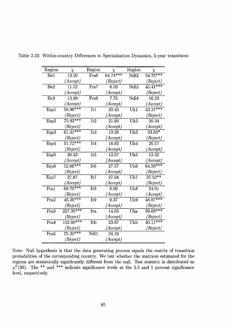
Table 2.23: Within-country Differences in Specialisation Dynamics, 5-year transitions
Region % Region X Region XBel 13.20
(Accept)Fra6 64.74***
(Reject)Ndl2 54.75***
(Reject)Be2 11.52
(Accept)Fra7 6.50
(Accept)Ndl3 45.41***
(Reject)BeS 13FW
(Accept)Fra8 7.75
(Accept)Ndl4 16.23
(Accept)Espl 58.96***
(Reject)I t l 30.43
(Accept)Ukl 43.21***
(Reject)Esp2 75.92***
(Reject)It2 21.93
(Accept)Uk2 20.34
(Accept)Esp3 61.31***
(Reject)It3 13.28
(Accept)Uk3 33.63*
(Reject)Esp4 51.72***
(Reject)It4 18.92
(Accept)Uk4 26.57
(Accept)Esp5 26.43
(Accept)It5 12.07
(Accept)Uk5 12.32
(Accept)Esp6 52.66***
(Reject)It6 27.57
(Accept)Uk6 64.50***
(Reject)Esp7 27.87
(Accept)Xt7 27.04
(Accept)Uk7 37.52**
(Reject)Fral 69.70***
(Reject)Its 8.00
(Accept)Uk8 24.91
(Accept)Pra2 46.26***
(Reject)It9 9.37
(Accept)Uk9 48.87***
(Reject)Fra3 227.35***
(Reject)Ita 14.03
(Accept)Uka 39.69***
(Reject)Pra4 102.80***
(Reject)Itb 23.87
(Accept)Ukb 40.11***
(Reject)Fra5 75.20***
(Reject)Ndll 24.19
(Accept)
Note: Null hypothesis is that the data generating process equals the matrix of transition probabilities of the corresponding country. We test whether the matrices estimated for the regions are statistically significantly different from the null. Test statistic is distributed as X^(20). The ** and *** indicate significance levels at the 2.5 and 1 percent significance level, respectively.
85
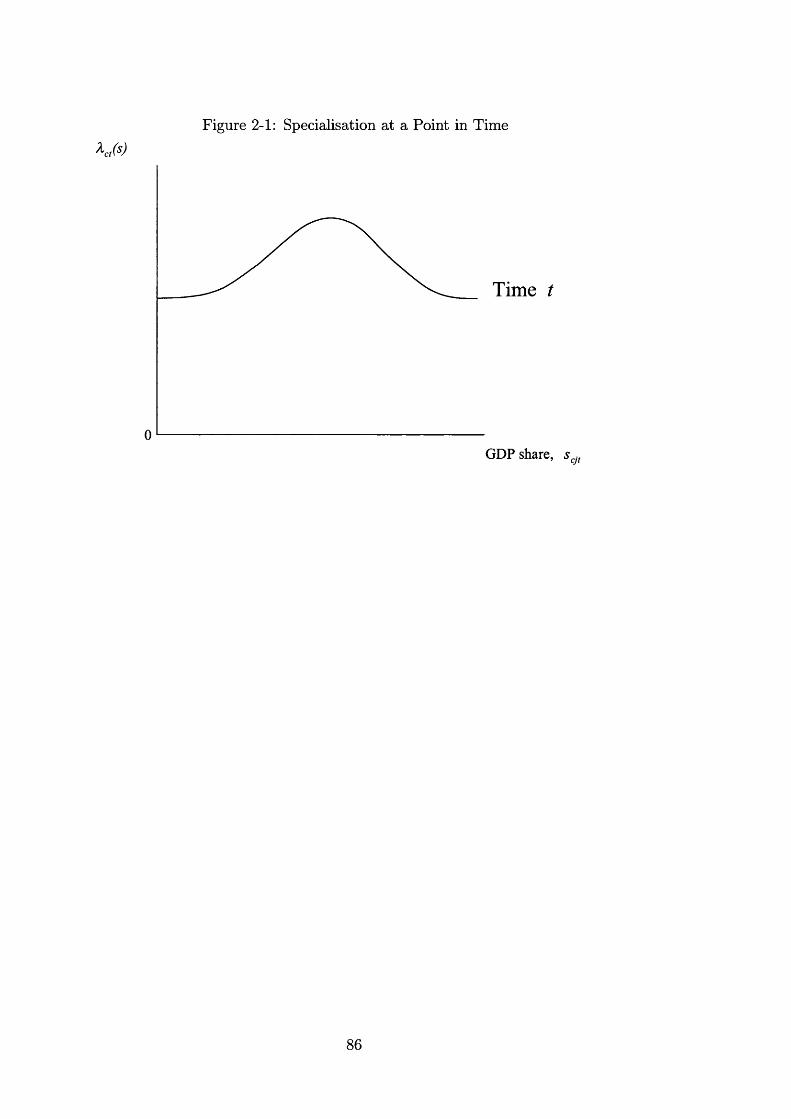
Figure 2-1: Specialisation at a Point in Time
Time t
0GDP share,
86

Figure 2-2: Specialisation Dynamics 1, Increased Specialisation
Time t+x
GDP share,
Time t
0 GDP share,
Figure 2-3: Specialisation Dynamics 2, Decreased Specialisation
Time /+T
GDP share, s.
Time t
0 GDP share,
87

2 . 1 0 A ppendix 2A
Table 2.24: Sample CompositionC oun try Sam ple A Sam ple B N um ber of N U TS-1 regionsBelgium 1975-95 1979-95 3 (bel-be3)Spain 1980-95 1980-94 7 (espl- esp7)France 1975-95 1977-94 8 (fral-fra8 )Italy 1975-95 1980-95 11 (ital-ita9, itaa/b)Luxembourg 1975-95 1979-90 1 (lux)Netherlands 1975-95 1977-95 4 (ndll-ndl4)United Kingdom 1975-86 1975-86 11 (ukl-uk9, uka/b)
Table 2.25: Industry Composition
C ode In d u s try D escrip tionA ggregate In d ustries1 Agricultural Sector: Food, Forestry and Fishery Products (Agric)2 Manufacturing Sector (M anuf)3 Services Sector: Market Services (Serv)D isaggregated M anufacturing In dustries4 Fuel And Power Products (Fuel)5 Ferrous And Non-Ferrous Ores And Metals, Other Than Radioactive (M etal)6 Non-Metallic Minerals And Mineral Products (M ineral)7 Chemical Products (C hem )8 Metal Products, Machinery, Equipment And Electrical Goods (M achine)9 Transport Equipment (Transp)11 Food, Beverages And Tobacco (Food)12 Textiles And Clothing, Leather And Footwear (Textile)13 Paper And Printing Products (P aper)14 Products Of Various Industries (O ther)15 Building And Construction (C onstr)

Table 2.26: Regions Included in the Sample
Code Description Code DescriptionBelgium LuxembourgBel Brussels Lux Luxembourg (Crand-Duche)Be2 Vlaams GewestBe3 Region Wallonne N etherlandsSpain Nidi North-NetherlandEspl Northwest (E) Nld2 East-NetherlandEsp2 Northeast (E) Nld3 West-NetherlandEsp3 Madrid Nld4 South-NetherlandEsp4 Centre (E) U nited KingdomEsp5 East (E) UKl North (UK)Esp6 South (E) UK2 Yorkshire And HumbersideEsp7 Canaries UK3 East MidlandsFrance UK4 East AngliaFral lle-De-France UK5 Southeast (UK)Pra2 Bassin Parisien UK6 Southwest (UK)Fra3 Nord-Pas-de-Calais UK7 West MidlandsPra4 East (F) UK8 Northwest (UK)Fra5 West (F) UK9 WalesFra6 Southwest (F) UKA ScotlandFra7 Centre-East (F) UKB Northern IrelandFraS MediterraneanItalyItal Northwest (1)lta2 Lombardialta3 Nordeast (1)lta4 Emilia-Romagnalta5 Centre (1)lta6 Laziolta7 Abruzzo-MoliseItaSlta9
Campania South (1)
Itaa SicilyItab Sardinia
89
C hapter 3
Factor Endowm ents and Production
in European Regions
3.1 Introduction^
“One of the best ways to understand how the international economy works is to
start looking at what happens inside nations... The data will be better and pose
fewer problems of compatibility, and the underlying economic forces will be less
distorted by government policies.”^
One of the most influential conceptual frameworks for theoretical and empirical work
in international trade is the Heckscher-Ohlin (HO) model. A key attraction is the model’s
ability to yield precisely formulated theoretical predictions which are amenable to direct
empirical testing. However, a number of cross-country studies have called into question
its empirical validity. For example, using data on cross-country trade in factor services,
Bowen et al. (1987), Trefler (1995) and Davis and Weinstein (2001) reject the HO model’s
assumptions of identical and homothetic preferences, identical technologies, and no barriers
to trade against a variety of more general alternatives.^ Similarly, when examining the cross
country relationship between industry-level production and factor endowments, Haxrigan
(1995) finds large within-sample prediction errors, while Harrigan (1997) provides evidence
As certified at the beginning of the thesis, this chapter is based on a co-joint research with my supervisor, Dr. Stephen Redding from the London School of Economics.
^Paul Krugman (1991b, page 3), cited in Bernstein and Weinstein (2002).^These more general alternatives allow, among other things, for cross-country differences in technology,
non-factor price equalization, trade costs and measurement error. See also Davis et al. (1997) and Gabaix (1997).
90

that non-neutral technology differences play an important role in explaining cross-country
variation in production structure.
This chapter examines the ability of the HO model to explain production patterns at the
regional level in Europe using a newly constructed panel dataset on output in 14 industries
and endowments of five factors of production for 45 NUTS-1 regions from 7 European coun
tries since 1975.' The use of regional data enables us to abstract from many of the reasons
advanced for the poor performance of the HO model at the country-level. For example, both
measurement error and technology differences are likely to be much smaller across regions
within Europe than for a cross-section of developed and developing countries. The ongoing
process of economic integration within the European Union means that it is an interesting
context within which to explore the relationship between production and factor endowments.
We control for exogenous variation in relative prices induced by European integration and
examine whether this process of international integration has strengthened or weakened the
relationship between production and factor endowments across regions within countries.
Much existing empirical work on the international location of production has, for reasons
of data availability, been concerned with the manufacturing sector. This paper explicitly
considers both manufacturing and non-manufacturing, where the latter accounts for more
than 70 percent of GDP in many NUTS-1 regions. We analyze production structure at two
alternative levels of industrial aggregation. First, we consider the three aggregate industries
of Agriculture, Manufacturing and Services. Second, we break out Manufacturing into 11
more disaggregated industries. We consider endowments of five factors of production: high-
education, medium-education, and low education individuals, physical capital, and land
area. The analysis focuses on patterns of production rather than trade, because the central
predictions of the HO model are for producer equilibrium and, in so doing, we abstract from
any violations of the model’s assumptions concerning consumer behaviour.^
The paper derives a general equilibrium relationship between production structure and
factor endowments that holds under the null hypothesis of the HO model with its assumptions
of identical prices and technologies. We compare this with the relationship that holds under
the more general alternative hypothesis of the neoclassical model of trade which allows for
regional variation in both relative prices and technology. We are able to explicitly test for
^NUTS stands for Nomenclature of Statistical Territorial Units. NUTS-1 regions are the first-tier of sub-national geographical units for which Eurostat collects data on the EU member countries. See Appendix A for more details concerning the data used.
^Three of the HO model’s four key theorems - the Rybczynski, Stolper-Samuelson, and Factor Price Equalization Theorems - require no assumptions about consumer preferences.
91

European regions whether the HO null is rejected against neoclassical alternatives, and use
our framework to examine the quantitative importance of factor endowments relative to
other considerations in explaining regional variation in production patterns.
While the use of regional data has many advantages, it means that the standard trade
assumption that endowments of factors of production are exogenous and perfectly immobile
across locations is less likely to apply. We show that the general equilibrium relationship
between production structure and factor endowments under the null hypothesis and the
corresponding relationship under the alternative hypothesis hold irrespective of whether
factors of production are perfectly immobile or perfectly mobile across locations ®
Factor mobihty does, however, change the interpretation of these relationships. If factor
endowments are exogenous and perfectly immobile across locations, the general equilibrium
relationship between production structure and factor endowments has a supply-side inter
pretation. Changes in factor endowments cause changes in production structure (production
moves in response to factor endowments). If factor endowments are mobile across locations,
they become potentially endogenous to production structure. In addition to the supply-side
interpretation given above, there is also a demand-side interpretation whereby changes in
production structure cause factor endowments to move across regions (factor endowments
move in response to production structure). Irrespective of whether the relationships we
estimate are demand-side, supply-side or a combination of both, we are able to test the
HO model’s predictions for the relationship between production and endowments against
those of the more general neoclassical model. Similarly, irrespective of which interpretation
applies, we can take the more general neoclassical model and examine the respective contri
butions of factor endowments and other considerations in statistically explaining variation
in production structure across European regions.
Our main empirical findings are as follows. First, the HO model provides an incomplete
explanation of patterns of production across European regions and is rejected against more
general neoclassical alternatives. Second, although the HO model is rejected, factor endow
ments remain statistically significant and quantitatively important in explaining production
structure within these neoclassical alternatives. Individual factor endowments are highly
statistically significant and including information on factor endowments reduces the model’s
within-sample average absolute prediction error by a factor of around three in Manufacturing.
®In practice, a wide range of evidence suggests that factor mobility across European regions is relatively low. This is particularly true across countries, where language and cultural differences act as barriers to labour mobility. However even within European countries, there is evidence that labour mobility is relatively low: see for example McCormick (1997) and Cameron and Muellbauer (1999) for evidence on the U.K.
92

Third, the pattern of estimated coefficients on factor endowments across industries is
generally consistent with economic priors regarding factor intensity. For example, physi
cal capital endowments are positively correlated with the share of Manufacturing in GDP
and negatively correlated with the shares of Agriculture and Services. Higher numbers of
medium education individuals relative to low education individuals are associated with a
lower share of Agriculture in GDP and a higher share of Manufacturing. Higher numbers of
high education individuals relative to medium education individuals are associated with a
lower share of Manufacturing in GDP and a higher share of Services.
Fourth, factor endowments are more successful in explaining patterns of production at the
aggregate level in Agriculture, Manufacturing and Services (where we have three industries
and either three or 5 factor endowments) than in disaggregated manufacturing industries
(where we have 11 industries and either three or 5 factor endowments). Within-sample av
erage absolute prediction errors are typically far larger in the disaggregated manufacturing
industries, and this is exactly as theory would predict. In the HO model with identical prices
and technology and with no joint production, patterns of production are only determinate if
there are at least as many factors of production as goods. Therefore, production indetermi
nacy provides one explanation for larger average absolute prediction errors in disaggregated
manufacturing industries. Another explanation, again consistent with the theory, is that
regional price and technology differences not controlled for in the right-hand side variables
are particularly large in individual manufacturing industries.
Fifth, we find no evidence that the process of increasing economic integration in Europe
has weakened or stengthened the relationship between patterns of production and factor
endowments across regions within countries. Our baseline econometric specification includes
country-year dununies so that the coefficients on factor endowments’ are identified solely
from variation across regions within countries. Examining within-sample prediction errors
for this specification reveals no systematic trend over time for either the three aggregate
industries or the 1 1 disaggregated industries within manufacturing.
The remainder of the chapter is organized as follows. Section 2 relates the chapter to the
existing literature. Section 3 introduces the theoretical framework and derives predictions for
production patterns under the HO null and the neoclassical alternative. Section 4 describes
the European regional production and factor endowments data. Section 5 discusses the
econometric specification. Section 6 presents the estimation results. Section 7 concludes.
93
3.2 Related Literature
A number of papers, including Leamer (1984), Bowen et al. (1987), Trefler (1995), Davis et
al. (1997), Gabaix (1997), and Davis and Weinstein (2001); have considered the relationship
between factor endowments and international trade in factor services at the country-level.
As discussed above, this literature typically finds that the HO model is rejected against more
general alternatives. Davis and Weinstein (2001) argue that, with a few plausible amend
ments, including cross-country differences in technology and a more flexible specification of
preferences, the HO model is consistent with international data on trade in factor services.
Although, the model is no longer Heckscher-Ohlin as traditionally conceived or strictly in
terpreted. The first paper to examine the empirical predictions of the HO model for the
location of production was Harrigan (1995), which used data on 10 manufacturing industries
in 20 OECD countries during 1970-85. Factor endowments were found to account for much
of the variation in output, although average prediction errors, expressed as a percentage of
actual production were around 40 percent. Physical capital was found to be an important
determinant of manufacturing output, although the effects of endowments of skilled and un
skilled labour were more ambiguous. Harrigan (1997) and Harrigan and Zakrajsek (2000)
use country-level data to estimate the neoclassical model of trade, which generalizes the HO
model to allow cross-country differences in technology and preferences. Harrigan (1997) finds
that both relative technology levels and factor endowments are important determinants of
patterns of production. Redding (2002) uses the neoclassical model to analyze the dynam
ics of countries’ production patterns, while Nickell et al. (2001) use a newly constructed
and disaggregated dataset on educational attainment in the OECD at the country level to
analyze the relationship between changing levels of educational attainment and production
patterns.
An emerging empirical literature has recently begun to examine the predictions of the
HO model using regional-data. Davis et al. (1997) analyze trade in factor services using
both country-level and Japanese regional data. The data on production in Japanese regions
are found to be consistent with factor price equalization. When the model is applied to data
on regional rather than country-level data on trade in factor services, the empirical results
are much more favourable. Bernstein and Weinstein (2002) use more disaggregated Japanese
regional data to examine the relationship between factor endowments and the location of
production. The data are again consistent with factor price equalization. However, there are
substantial within-sample prediction errors, which Bernstein and Weinstein (2002) interpret
as evidence of production indeterminacy. Hanson and Slaughter (2002) use data on immi
94

gration in US States to test a generalization of the Rybczynski Theorem, which predicts that
regions will accommodate immigrant inflows by changes in output mix rather than changes
in relative factor prices/ Changes in state output mix are found to broadly match changes
in state endowments. Moreover, the variation in factor intensities across US States is found
to be consistent with relative factor price equalization. Assuming that each US State is
small, the latter is a sufficient condition for changes in endowments to be accommodated by
changes in output mix.
A body of empirical work has sought to characterize the nature and evolution over time of
specialisation in Europe using country-level data: see, for example, Amiti (1999), Brülhart
(2000), Midelfart-Knarvik, Overman, Redding, and Venables (2000) and Proudman and
Redding (1998, 2000). Amiti (1999) finds evidence of increasing specialisation in Europe
using production and employment data, while Brülhart (2000) finds that specialisation has
increased in employment terms but remained roughly unchanged in export terms. Using
export data and statistical techniques for modelling the evolution of entire distributions,
Proudman and Redding (1998, 2000) find evidence of substantial changes in patterns of
specialisation over time. In contrast to all of these papers, which employ country-level data.
Chapter 2 characterizes specialisation at the regional-level in Europe for the same sample
considered here. We refer to chapter 2 for related work on specialisation at the regional level
in Europe (see Combes and Overman, 2003, for an extensive review).
Finally, the chapter relates to a recent empirical literature on economic geography (see
Overman et al. 2002, for a survey on this literature). Davis and Weinstein (1999, 2003) use
data on Japanese regions and on a cross-section of countries, respectively, to test for a ‘home
market’ or ‘magnification’ effect. That is, in models of economic geography, the presence of
increasing returns to scale and transport costs means that an increase in expenditure on a
good has a more than proportionate effect on domestic production of the good. The same is
not true in the constant returns to scale world of HO, and this provides the basis for an iden
tifying restriction. Using country-level data on OECD manufacturing industries, Davis and
Weinstein (2003) investigate the existence of home market effects from idiosyncratic demand
on the pattern of production with a framework that nests a conventional Heckscher-Ohlin
model (based on comparative advantage) with a model of economic geography. They find
evidence suggesting that home market effects are important for a broad segment of OECD
manufacturing. The analysis of regional-level data on Japanese manufacturing industries in
Davis and Weinstein (1999) also reveals evidence of economic geography effects in eight out
^See Gandal, Hanson, and Slaughter (2002) for a related analysis of immigration in Israel.
95
of 19 industries, and these effects are shown to be quantitatively important. Brülhart and
Torstensson (1996) consider the effects of increasing integration on the location of increasing
returns to scale industries and the pattern of international trade. Data on 11 European coun
tries provide some empirical support for the predictions of an economic geography model:
employment in increasing returns to scale industries tends to be concentrated at the centre
of the EU and intra-industry trade is relatively low in these industries. Midelfart-Knarvik,
Overman, and Venables (2000b) employ European country-level data to analyze the deter
minants of specialisation in manufacturing industries during 1970-97. A role is found for
both the considerations of traditional trade theory (e.g., factor endowments and factor in
tensities) and those emphasized by the economic geography literature (e.g., geographical
proximity and forward/backward linkages).
3.3 Theoretical Framework
The theoretical framework is provided by the neoclassical theory of trade and production
(see, in particular, the exposition in Dixit and Norman, 1980). Regions are indexed by
z G {1,..., %}; goods by j G {1,..., A}; factors of production by z G {1,...,M }; and time
by t. Production is assumed to occur under conditions of perfect competition and constant
returns to scale.^ The neoclassical model allows for regional differences in factor endowments
as well as region-industry differences in technology and relative prices. The HO model
corresponds to a special case where all regions have identical relative prices and technology,
and is therefore nested by the neoclassical model.
General equilibrium in production may be represented using the revenue function {pzt, Vzt),
where Pzt denotes a region’s vector of relative prices and Vzt is its vector of factor endowments.
Under the assumption that the revenue function is twice continuously differentiable, we ob
tain determinate predictions for a region’s vector of profit-maximizing net outputs VziPzt: ^zt)
which equals the gradient of {Pzu^zt) with respect to Pzt-^ We allow for Hicks-neutral
® While analysis of the neclassical model typically focuses on the perfectly competitive case, it is also possible to analyze imperfect competition as discussed in Helpman (1984).
sufficient condition for the revenue function to be twice continuously differentiable and production patterns to be determinate is that there are at least as many factors as goods: M > N. In the HO model where relative prices and technology are identical, production levels may still be determinant when N > M 1Î there is joint production. More generally in the neoclassical model, differences in technology and relative prices may render production determinant when N > M. The potential existence of production indeterminacy is really an empirical issue which we investigate below for alternative numbers of goods and factors. If production indeterminacy exists, the equation that we derive under the null linking production and factor endowments will be relatively unsuccessful in explaining regions’ production patterns, in terms of having statistically insignificant right-hand side variables, low explanatory power and large within-sample
96
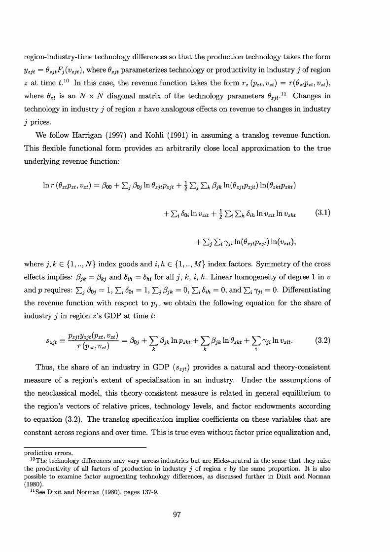
region-industry-time technology differences so that the production technology takes the form
Vzjt = OzjtFj{vzjt), where 9zjt parameterizes technology or productivity in industry j of region
z at time In this case, the revenue function takes the form [pzt.Vzt) = f'{0ztPzt,Vzt),
where is an AT x diagonal matrix of the technology parameters 9zjt-^ Changes in
technology in industry j of region z have analogous effects on revenue to changes in industry
j prices.
We follow Harrigan (1997) and Kohli (1991) in assuming a translog revenue function.
This flexible functional form provides an arbitrarily close local approximation to the true
underlying revenue function:
In r (OztPzt, Vzt) = /?oo + E j A j In dzjtPzjt + \ E j E& Pjk ^-^{OzjtVzjt) ^^{OzktPzkt)
+ Ez In Vzit + Ez E/z ^ih fn Vzit In Vzht (3 1)
"b Eji Ez 'yji ^^{PzjtPzjt) fn(u2z(),
where j , k G {1,.., N } index goods and z, A G {1,.., M } index factors. Symmetry of the cross
effects implies: l3jk = Pkj and 6ih = Shi for all j , k, z, h. Linear homogeneity of degree 1 in z;
and p requires: E j 1, Ez <0z = 1, E j ftfc = 0, Ez Sih = 0, and Ez Iji = 0- Differentiating the revenue function with respect to we obtain the following equation for the share of
industry j in region z ’s GDP at time t\
Szjt = ^ Inpzkt + ^n Ozkt + Tz* (3.2)V [Pzt, Vzt) k k i
Thus, the share of an industry in GDP {Szjt) provides a natural and theory-consistent
measure of a region’s extent of specialisation in an industry. Under the assumptions of
the neoclassical model, this theory-consistent measure is related in general equilibrium to
the region’s vectors of relative prices, technology levels, and factor endowments according
to equation (3.2). The translog specification implies coefficients on these variables that are
constant across regions and over time. This is true even without factor price equaflzation and.
prediction errors.^°The technology differences may vary across industries but are Hicks-neutral in the sense that they raise
the productivity of all factors of production in industry j of region z by the same proportion. It is also possible to examine factor augmenting technology differences, as discussed further in Dixit and Norman (1980).
^^See Dixit and Norman (1980), pages 137-9.
97
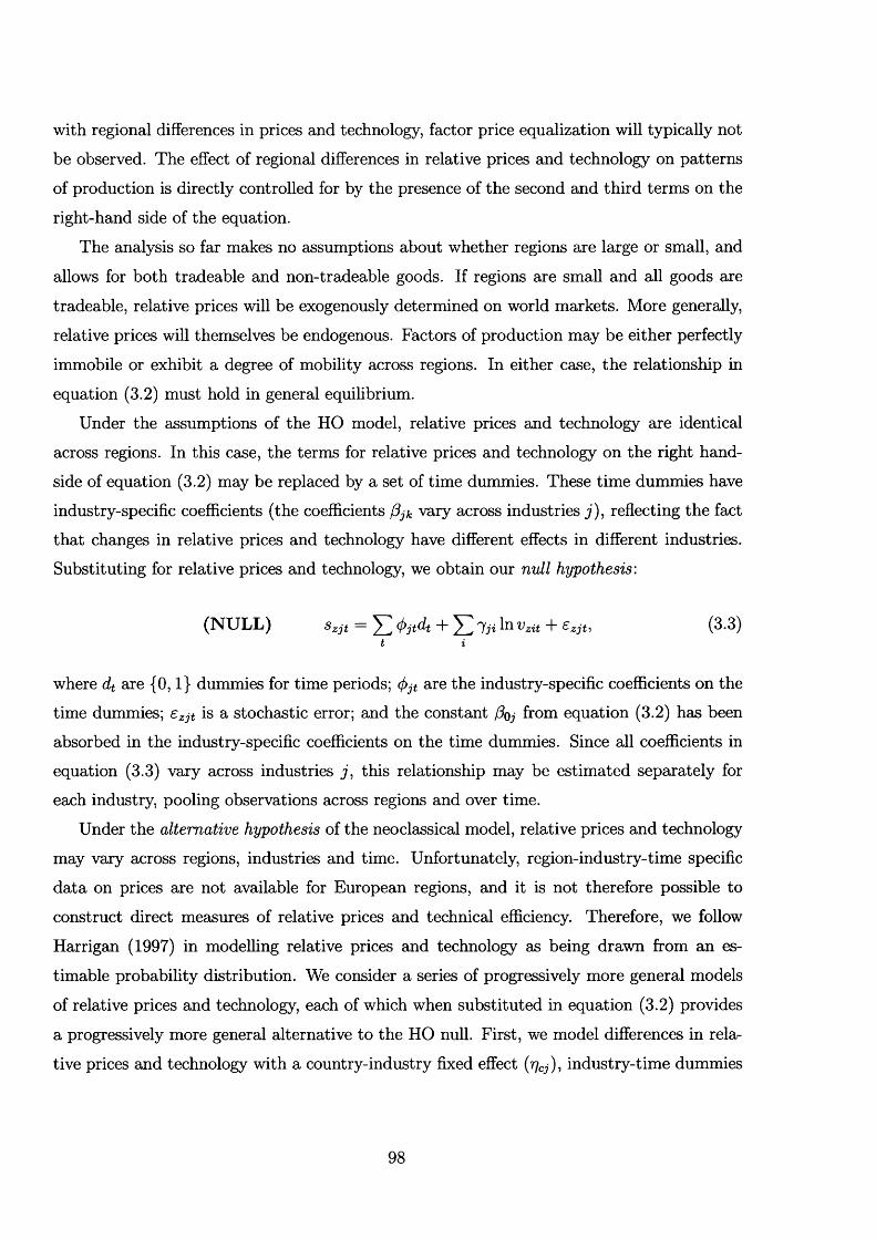
with regional differences in prices and technology, factor price equalization will typically not
be observed. The effect of regional differences in relative prices and technology on patterns
of production is directly controlled for by the presence of the second and third terms on the
right-hand side of the equation.
The analysis so far makes no assumptions about whether regions are large or small, and
allows for both tradeable and non-tradeable goods. If regions are small and all goods are
tradeable, relative prices will be exogenously determined on world markets. More generally,
relative prices will themselves be endogenous. Factors of production may be either perfectly
immobile or exhibit a degree of mobility across regions. In either case, the relationship in
equation (3.2) must hold in general equilibrium.
Under the assumptions of the HO model, relative prices and technology are identical
across regions. In this case, the terms for relative prices and technology on the right hand-
side of equation (3.2) may be replaced by a set of time dununies. These time dummies have
industry-specific coefficients (the coefficients (3jk vary across industries j) , refiecting the fact
that changes in relative prices and technology have different effects in different industries.
Substituting for relative prices and technology, we obtain our null hypothesis:
(N U L L ) ^ z j t ~ ^ y T ^ ^ z i t T ^ z j t t (^•^)t i
where dt are {0 , 1 } dummies for time periods; (f)jt are the industry-specific coefficients on the
time dummies; Szjt is a stochastic error; and the constant /Sqj from equation (3.2) has been
absorbed in the industry-specific coefficients on the time dummies. Since all coefficients in
equation (3.3) vary across industries j , this relationship may be estimated separately for
each industry, pooling observations across regions and over time.
Under the alternative hypothesis of the neoclassical model, relative prices and technology
may vary across regions, industries and time. Unfortunately, region-industry-time specific
data on prices are not available for European regions, and it is not therefore possible to
construct direct measures of relative prices and technical efficiency. Therefore, we follow
Harrigan (1997) in modelling relative prices and technology as being drawn from an es
timable probabihty distribution. We consider a series of progressively more general models
of relative prices and technology, each of which when substituted in equation (3.2) provides
a progressively more general alternative to the HO null. First, we model differences in rela
tive prices and technology with a country-industry fixed effect {rjcj), industry-time dummies
98
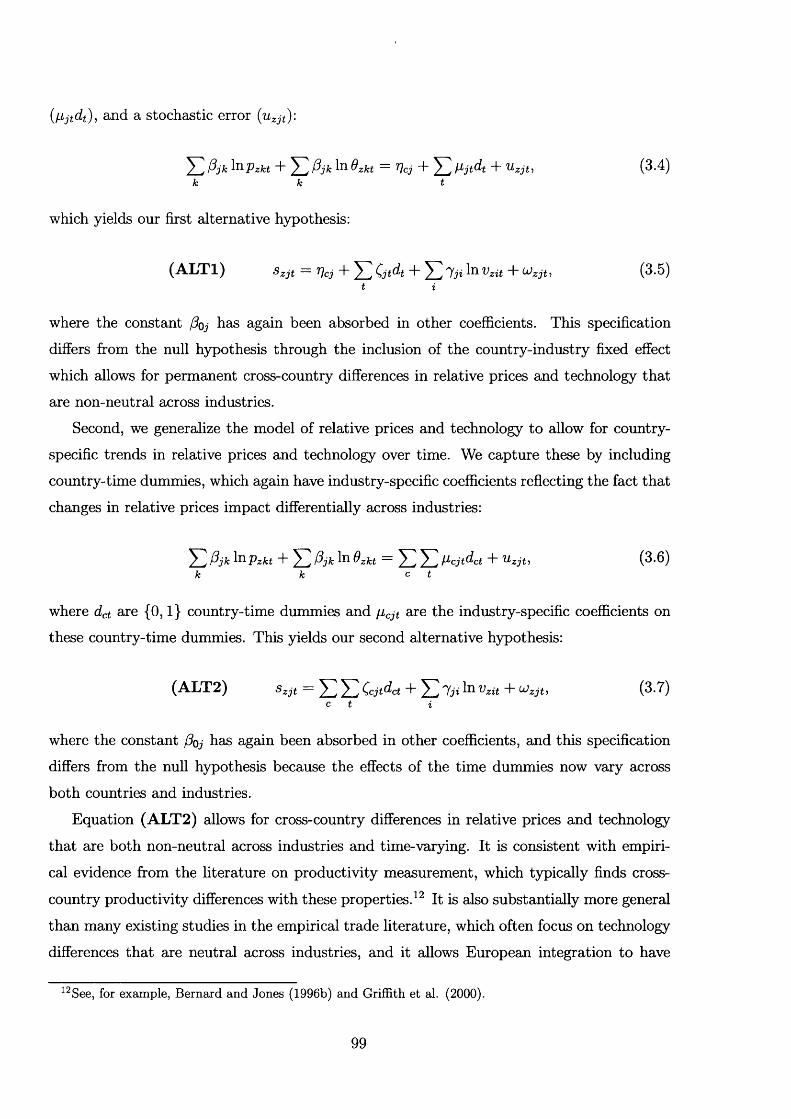
( l i j t d t ) , and a stochastic error (uz j t ) :
^ V Pik 111Pzkt "h ^ ] Pjk ^zkt Vcj “t“ ^ y l^jjdt Uzj t i ( 3 - 4 )k k t
which yields our first alternative hypothesis;
(A L T l) Szjt = T]cj + ^ Cjtdt + ^ 7 ji In Vzu + ujzjt, (3.5)t i
where the constant poj has again been absorbed in other coefficients. This specification
differs from the null hypothesis through the inclusion of the country-industry fixed effect
which allows for permanent cross-country differences in relative prices and technology that
are non-neutral across industries.
Second, we generalize the model of relative prices and technology to allow for country-
specific trends in relative prices and technology over time. We capture these by including
country-time dummies, which again have industry-specific coefficients reflecting the fact that
changes in relative prices impact differentially across industries:
^ V Pjk ^^Pzkt "b ^ Pjk ^zkt ^ ^ ] P'cjtdct T '^zjti (3.6)k k c t
where dct are {0 , 1 } country-time dummies and ficjt are the industry-specific coefficients on
these country-time dummies. This yields our second alternative hypothesis:
(ALX2 ) Szjt — ^ ^ V Ccjtdct T ^ ] 'ïji ill ' zit T ^zjti (3.7)c t i
where the constant Poj has again been absorbed in other coefficients, and this specification
differs from the null hypothesis because the effects of the time dummies now vary across
both countries and industries.
Equation (ALT2) allows for cross-country differences in relative prices and technology
that are both non-neutral across industries and time-varying. It is consistent with empiri
cal evidence from the literature on productivity measurement, which typically finds cross
country productivity differences with these properties. It is also substantially more general
than many existing studies in the empirical trade literature, which often focus on technology
differences that are neutral across industries, and it allows European integration to have
^^See, for example, Bernard and Jones (1996b) and Griffith et al. (2000).
99
different effects on relative prices across countries.
Third, we extend the model of relative prices and technology further to allow for per
manent region-industry specific differences in relative prices and technology country-
specific trends in relative prices and technology over time {dct) and a stochastic error {uzjt):
^ Pjk ^^Pzkt "h ^ In 9zkt Pzj ^ ^ ] P'cjtdct '^zjti (3-8)k k c t
which yields our third alternative hypothesis:
(■^LX3) zjt Vzj Ccjtdct Tn Vzit ^zjti (3-9)c t i
where the constant Pqj has again been absorbed in other coefficients. This specification
differs from the null hypothesis, because of both coefficients on the time dununies that vary
across countries and industries, and because of the inclusion of a region-industry fixed effect.
The null hypothesis is derived directly from the HO model with its assumption of identical
relative prices and technology. Similarly, each of the alternative hypotheses is derived directly
from the neoclassical model and involves making progressively more general assumptions
about relative prices and technology. Both variable choice and functional form are shaped
by the underlying theory. Hence, under the assumptions of the null hypothesis or a particular
alternative hypothesis, the relevant relationship may be given an economic interpretation.
In particular, under the assumptions of the null hypothesis^ the coefficients on factor
endowments (7 ^ ) in (N U LL) are directly related to the Rybczynksi derivatives of HO theory
- the general equilibrium relationship between production and factor endowments holding
constant relative prices and tech n o lo g y .A s discussed above, if factor endowments exhibit a
degree of mobility across regions, the Rybczynski derivatives capture a relationship between
output and factor endowments that must hold in general equilibrium, but that may be given
either a demand-side or supply-side interpretation. In relating the coefficients 7 % to the
Rybczynksi derivatives, we are not asserting the existence of a causal relationship between
exogenous changes in factor endowments and endogenous changes in production, but are
instead examining a relationship that holds in equilibrium (examining the equilibrium value
of the derivatives).
The factor intensities of industries are directly captured in our analysis by the estimated
Formally, the Rybczynski derivatives are dyj{p,v)/dv\ = d^r{p,v)/dpjdv\ = d^r{p,v)/dv\dpj for all i. Differentiating with respect to v\ in equation (N U LL) and rearranging, d^ln{r{p,v))/dpjdv\ = 7ji/(pjVi) so that the Rybczynski derivatives take the same sign as the 7 j j.
100

coefficients (7 ^ ) on factor endowments. With large numbers of factors (M) and goods (N),
many conventional definitions of factor intensity (such as the ratio of use of one factor
of production to another) are problematic. Nevertheless, the fact that in our approach the
estimated coefficients on factor endowments are directly linked to the Rybczynski derivatives
of HO theory means that they can be related to natural measures of factor intensity.
For example, with M = N, a, positive value of a Rybczynski derivative for factor i and
good j imphes that, if the price of factor i increases by one unit and all other factor prices
are adjusted to keep other goods’ unit costs unchanged, the unit costs of production for
good j must rise. In this sense, good j is intensive in the use of factor i relative to the
economy as a whole when d^r{p,v)/dpjdvi and hence j j i is positive . W ith M > N, there
will generally be more than one set of values for other factor prices that leave other goods’
unit costs unchanged. Nonetheless, a natural measure of factor intensity still exists based on
the Rybczynski derivatives themselves, whereby good j is said to be relatively more intensive
in factor i than the average if d^r{p,v)/dpjdvi and hence j j i is positive.
Intuitively, we do not try to construct conventional measures of factor intensity which
are often problematic with large numbers of factors and goods, but instead directly estimate
the relationship between production and factor endowments. Under the HO null, factor
intensities are captured in the estimated coefficients on factor endowments. The fact that
natural measures of factor intensity are defined relative to the whole structure of general
equilibrium when there are large numbers of factors (M) and goods (N) is directly related
to the way in which the theorems of the 2x2x2 HO model now hold in a weakened form as
averages and correlations.^^
Note that the estimated coefficients on factor endowments {'jji) in (N U LL) only cor
respond to Rybczynski derivatives if the assumptions of the HO null are satisfied. Under
the alternative hypothesis of the more general neoclassical model, (N U LL) is mis-specified
because it omits terms capturing regional variation in relative prices and technology. In
general, these terms will be correlated with factor endowments and their omission will give
rise to omitted variables bias and inconsistent estimates of the jji. Only by including these
additional terms, as for example in (A LT 2 ), can consistent estimates of the j j i be obtained.
We investigate the importance of regional variation in relative prices and technology by
comparing the results of estimating (N ULL) to those from estimating the three alternative
specifications (A LT1)-(A LT3). We compare the specifications along four main dimensions.
' See Dixit and Norman (1980), pages 53-9.^^See, for example, Dixit and Norman (1980), Chapter 4 of this thesis, and Ethier (1984), Sections 6 & 7.
101
First, since the null is nested by each of the alternatives, a test of the statistical significance
of the additional terms capturing regional variation in relative prices and technology provides
a formal test of the null against each of the more general alternatives. Second, we investigate
the importance of the omitted variables bias by considering how the estimated coefficients
on factor endowments change as we move to progressively more general models of relative
prices and technology. Third, we examine the quantitative importance of factor endowments
relative to other considerations in explaining regional variation in production structure.
Fourth, we evaluate the empirical performance of the null and alternative hypotheses using
a number of model specification tests.
Finally, it is worth noting that factor mobility does, however, change the interpretation
of these relationships. If factor endowments are exogenous and perfectly immobile across
locations, the general equilibrium relationship between production structure and factor en
dowments has a supply-side interpretation. Changes in factor endowments cause changes in
production structure (production moves in response to factor endowments). If factor endow
ments are mobile across locations, they become potentially endogenous to production struc
ture. In addition to the supply-side interpretation given above, there is also a demand-side
interpretation whereby changes in production structure cause factor endowments to move
across regions (factor endowments move in response to production structure). Irrespective
of whether the relationships we estimate are demand-side, supply-side or a combination of
both, we are able to test the HO model’s predictions for the relationship between production
and endowments against those of the more general neoclassical model. Similarly, irrespective
of which interpretation applies, we can take the more general neoclassical model and examine
the respective contributions of factor endowments and other considerations in statistically
explaining variation in production structure across European regions.
3.4 D ata Description
As discussed in Chapter 2, the main source of data is the Regio dataset compiled by the
European Statistics Office (Eurostat). We analyze patterns of production across 14 industries
in 45 NUTS-1 regions from 7 European countries since 1975. The number and size of NUTS-
1 regions varies across European countries. This is perfectly consistent with our model, and
the variation in size will be exploited in tests of the linear homogeneity restrictions implied
by theory.
Patterns of production are analyzed at two alternative levels of aggregation. First, we
102
consider three aggregate (one-digit) industries: Agriculture, Manufacturing and Services.
Second, we exploit more disaggregated information on individual industries within Manufac
turing. These are mainly two-digit industries and include, for example. Textiles Sz Clothing
and Chemicals. Again, full details are given in Appendix 3A.
The Regio dataset provides information on industry value-added and GDP by region,
from which we compute the share of each sector in GDP. It also provides information on
three broad factor endowments: total population, physical capital and land area.^® These
data are merged with information on educational attainment at the regional level from
individual country labour force surveys. This enables us to disaggregate the population
endowment into low, medium and high education. The definitions we employ are standard
in the labour market literature (see, for example, Nickell and Bell, 1996, and Machin and
Van Reenen, 1998). ‘Low education’ corresponds to no or primary qualifications, ‘medium
education’ denotes secondary and/or vocational qualifications, and ‘high education’ is college
degree or equivalent.
The length of the time-series available varies with the level of industrial aggregation,
whether or not we use the information on educational attainment, and with the country
considered. In order to exploit all of the information available, we consider two estima
tion samples. First, at the level of the three aggregate industries and for the three factor
endowments (population, physical capital and land area), we have an unbalanced panel of
811 observations per industry on the 45 regions during approximately 1975-95 (Sample A).
Second, for the disaggregated manufacturing industries and for the 5 factor endowments
(low education, medium education, high education, physical capital and land area), we have
an unbalanced panel of 696 observations per industry from approximately 1980 onwards
(Sample B). Full details of the composition of each sample are given in Appendix A.
Table 3.1 examines variation in the three broad factor endowments (Population, Capital
and Land) across regions at a point in time and within regions over time. The sample
includes both UK5 (with a population of more than 16 million in 1985) and Luxembourg
(with a population of just over 350,000 in 1985). Land area varies from around 16,000
hectares in Bel (Brussels) to 21 million hectares in Es4 (Centre). While population declined
in some regions, such as UKl (North), it rose in others, such as UK6 (South-West). All
regions exhibit an increase in the real stock of physical capital over time, although the rate
of increase varies across regions.
also experiment with using data on arable land area to control for variation in land quality. ^^See Appendix 3A for further information concerning the data used.
103

< T able 3.1 a b o u t h ere>
In Table 3.2 we report regional educational attainment as a percentage of the population
for the years 1985 and 1995. It is well known from the labour market literature that the
sample period was one of rising educational attainment in European countries (see, for
example, Nickell and Bell 1996 and Machin and Van Reenen 1998). W ith the exception of
Bel (Brussels), all regions in Table 3.2 experience a rise in the share of the population with
high education. However the rate of increase varies substantially, even across regions even
within a country. For example, in Esp2 (North-East) the high education share rises by over
70 percent, while in the neighbouring region of Espl (North-West) the proportional rate of
increase is approximately 40 percent. Multiplying the percentage shares in Table 3.2 by the
population levels reported in Table 3.1, we obtain regions’ endowments of low, medium and
high education individuals.
< T able 3.2 a b o u t h ere>
3.5 Econometric Specification
Our null and alternative specifications are derived directly from the structure of the theo
retical model, as explained above, and are reproduced below:
S z j t ^ > 4^ jtd t T ^ ] ' y g In T ^ z j t it i
S z j t ~ Vcj "b ^ ] C j t^ t T ^ ] H ji '^zit ^ z j t i t i
S z j t — ^ 2 C c jtd c t d" y ] 'Jji In V zit T ^ z j t ic t i
Szj t ~ Vzj T y ] y y Ccjtdct "b y ' j j i i n Vzu "b (jJzjt'
(N U LL) Szjt
(A L T l) Szjt
(ALT2) Szj t
(ALT3) Szj tc t
Since all coefficients vary across industries, specifications are estimated separately for each
industry, pooling observations across regions and over time.
As we move from the null to each of the alternative specifications, we change the source
of variation in the data used to identify the coefficients on factor endowments (jji). For
example, in (N U LL), the inclusion of time dummies in each industry regression means
that we abstract from any common trend in factor endowments over time across all regions,
and the ^ji are identified from variation across regions at a point in time and differential
variation within regions over time. In (ALT2), the inclusion of country-time dununies means
104

that we abstract from any common trend in factor endowments across all regions within a
country, and the 7 ^ are identified from variation across regions within a country at a point
in time and differential variation within regions over time. If the assumptions of the HO
model are satisfied, the additional terms included in specifications (A LT1)-(A LT3) should
be statistically insignificant, and the estimated 7 , should remain unchanged, as we move
to progressively more general models of relative prices and technology and exploit different
sources of variation in the data.
However, as we move from (ALT2) to (ALT3), the within groups transformation due to
the inclusion of the regional fixed effect {rjzj) can greatly exacerbate any attenuation bias from
measurement error in the independent variables (see, in particular, Griliches and Hausman
1986). Intuitively, the extent of ‘within’ or time-series variation in factor endowments due
to true variation in the independent variables may be small relative to the variation due
to measurement error. This is likely to be a particular problem in the present application
because the extent of time-series variation in some of our factor endowments (in particular
land area and, to a lesser extent, population) is limited.
We address this problem in two ways. First, we exploit disaggregated data on the ed
ucational attainment of the population and on arable land area. The resulting measures
of factor endowments control for variation in levels of skills and land quality, and exhibit
greater differential variation over time within regions. Second, following Griliches and Haus
man (1986), we consider the use of first-difference estimators. The longer the interval of
time over which we difference the data, the greater the amount of true variation in factor
endowments relative to that due to measurement error. Hence, the attenuation bias due to
measurement error should be smaller using longer differences, and we analyze the results of
10-year difference estimators. We thus obtain a fourth alternative specification:
(ALT4) A-\oSzjt = ^ Cjtdt + ^ 7 ji'^io In Vzu + 4’zjt,t i
where differencing eliminates the regional fixed effect {rjzj)- In taking long differences, we
substantially reduce the sample size and, therefore, we concentrate on a specification with
only industry-specific coefficients on the time dummies.
In comparing the results of estimating the null and alternative specifications, we also make
use of two model specification tests. The first of these focuses on the time-series properties
of the model. By construction, the share of sector j in GDP (szjt) is bounded between 0 and
100 per cent, and is therefore 1(0). However, in any finite sample, GDP shares may be 1(1).
105

This is particularly true of our sample period (1975-95) which, in general, is characterized
by a secular decline in the GDP shares of Agriculture and Manufacturing combined with a
secular rise in the share of Services. Similarly, a region’s population and physical capital
endowments may be 1(1). In this case, the static levels regressions (N U LL )-(A LT 3) should
be interpreted as cointegrating relationships between a sector’s share of GDP and factor
endowments. Under this interpretation, the residuals should be 1(0) if the assumptions
underlying a particular specification are satisfied. Therefore, we make use of the panel data
unit root test of Maddala and Wu (1999) to test for the stationarity of the residuals.
Second, neoclassical trade theory assumes that the production technology is constant
returns to scale and hence that the revenue function in equation (3.1) is homogeneous of
degree one in factor endowments. Therefore, a test of the null hypothesis that the sum
of the estimated coefficients on factor endowments is equal to zero provides another model
specification test {Ylilji = 0 ).
3.6 Empirical Results
We begin in Colunm (1 ) of Tables 3.3-3.5 by reporting the results of estimating the HO
specification (N U LL) for the aggregate industries (Agriculture, Manufacturing and Services)
using our three broad measures of factor endowments (population, physical capital and land
area). We find a statistically significant relationship between regional patterns of production
and factor endowments and, from the regression R^, the HO specification explains some
30-45 percent of the variation in production patterns across European regions. We also
find statistically significant effects of the year dummies, consistent with an important role
for common changes in relative prices and technology.
< Tables 3.3-3.5 about here>
In Column (2) of Tables 3.3-3.5, we relax the assumption of identical relative prices and
technology in the first alternative specification (A L T l). The country fixed effects are highly
statistically significant, as shown in the first of the F-statistics reported in Colunm (2). The
of the regression rises substantially, and by more than one third in both Agriculture and
^®The Maddala and Wu or Fisher test statistic is based on the sum of the p-values from conventional Augmented Dickey Fuller (ADF) tests on the residuals for each cross-section unit z € Z. It can be shown that —2 111 fz has a distribution with 2Z degrees of freedom. This test statistic has a direct intuitiveinterpretation, is valid for unbalanced panels and has attractive small sample properties (Maddala and Wu 1999). Other analyses of unit roots and cointegration in a panel data context include Im et al. (2003), Levin and Lin (1992), Pedroni (1999), Pesaran et al. (1998) and Quah (1994).
Except where otherwise indicated, statements about statistical significance refer to the 5% level.
106

Manufacturing. The pattern of estimated coefficients on factor endowments also changes
and moves more in line with economic priors concerning factor intensity. For example, in
Agriculture the coefficient on physical capital switches from being positive and statistically
significant to negative and statistically significant, while in Manufacturing the coefficients
on physical capital and population increase by an order of magnitude. The statistical signif
icance of the country fixed effects rejects the null hypothesis of the HO model; the rise in
suggests that the additional terms capturing variation in relative prices and technology are
quantitatively important; and the change in the estimated pattern of coefficients suggests
the importance of including these controls in identifying the relationship between production
patterns and factor endowments.
In Column (3) of Tables 3.3-3.5, we generalize the model of relative prices and technology
further and consider specification (A LT 2 ) which allows for different cross-country trends in
relative prices and technology over time. In the HO specification (N U LL), each industry
regression includes a set of time dummies. In moving from (N U LL) to (A LT2), we retain
these time dummies (which will capture effects for the omitted country) and augment the
regression specification with country-time dummies for all countries except one. The first
of the F-statistics in this column of the tables reports the results of a test whether the
coefficients on the additional country-year dummies are statistically significantly different
from zero. In all industries, the country-year dummies are highly statistically significant,
and the HO specification (N U LL) is again rejected against the more general alternative.
Comparing Columns (2 ) and (3), the pattern of estimated coefficients on factor endow
ments remains stable between specifications (A L T l) and (ALT2). This suggests that con
trolling for different cross-country trends in relative prices and technology does not substan
tially alter the relationship between factor endowments and regional production patterns,
and that it is far more important to control for permanent cross-country differences in relative
prices and technology (the move from (N U LL) to (A L T l)).
The values of the estimated coefficients on factor endowments in (ALT2) are gener
ally consistent with economic priors. Population endowments are positively correlated with
specialisation in Services and negatively correlated with specialisation in Manufacturing.
Greater endowments of physical capital are associated with a higher share of Manufacturing
in GDP and a lower share of Agriculture and Services. Land area is positively related to
specialisation in Agriculture and Manufacturing and negatively related to specialisation in
Services. W ith the exception of the coefficient on population in the regression for Agriculture,
all estimated coefficients are statistically significant at the 5 percent level.
107

Column (4) of Tables 3.3-3.5 reports the results of extending the model of relative prices
and technology further to include a region-industry fixed effect in specification (ALT3).
Here, the pattern of estimated coefficients changes substantially and no longer has a plausi
ble economic interpretation. For example, land area is negatively correlated with the share
of Agriculture in GDP, while endowments of physical capital are positively and statistically
significantly correlated with specialisation in Agriculture. Since there is almost no time-
series variation in land area (see Table 3.2), it is unclear how appropriate or meaningful
this econometric specification is. The parameters of interest are being identified from devi
ations from time means for individual regions, which in all cases are extremely small and
in many cases are literally zero. It is plausible that the change in the estimated coeffi
cients between (A LT 2 ) and (ALT3) is largely driven by measurement error (Griliches and
Hausman 1986). We investigate this possibihty further below, where we disaggregate factor
endowments (thereby introducing more time-series variation) and explore the results of long
differences estimation.
Tables 3.3-3.5 also report the sum of the estimated coefficients on factor endowments in
each industry and the results of a test whether the revenue function is linearly homogenous
of degree one in factor endowments (a test of the null hypothesis that JZi Iji = 0). Although
the sum of the estimated coefficients is close to zero (in several cases, the order of magni
tude is 1 0 “^), the null hypothesis is frequently rejected at conventional levels of statistical
significance. There is some evidence of increasing returns to scale in Manufacturing, where
the sum of the estimated coefficients is strictly greater than zero in all specifications.
Our other model specification test examines the stationarity of the residuals using the unit
root tests of Maddala and Wu (1999). In Agriculture we are able to reject the null hypothesis
of a unit root in the residuals in all specifications, while in Services and Manufacturing we are
unable to reject the null hypothesis in half the specifications. Taken together, these results
provide some evidence of model mis-specification. Two possible explanations for the non-
stationarity of the residuals are the omission of information on relevant factor endowments
or time-varying regional price and technology differences that have not been controlled for
(both of which will be included in the error term).
Table 3.6 investigates the first of these possibilities by introducing information on edu
cational attainment and land quality. The availability of the educational attainment data
reduces the sample size to 696 observations per industry (Sample B).^° In the interests of
* The model in Tables 3.3-3.5 was re-estimated for the reduced sample; this yields very similar results to those reported in the paper.
108

brevity, we only report the results for specifications (ALT2) and (A LT3). In both cases,
as shown in the first F-statistic reported in the table, we reject the HO null against the
more general neoclassical alternative, and we begin by considering the estimation results for
specification (ALT2).
< T able 3.6 a b o u t h ere>
The estimated coefficients on physical capital are very similar to before, while the arable
land coefficients closely resemble those on total land area. In addition, we find highly sta
tistically significant effects of education endowments. Greater endowments of low-education
labour are positively and statistically significantly correlated with specialisation in Agricul
ture, while endowments of medium-education labour are negatively and statistically signifi
cantly correlated with the share of Agriculture in GDP. There is a positive and statistically
significant relationship between endowments of medium-education labour and Manufactur
ing’s share of GDP, while the relationship with endowments of high-education labour is
negative and statistically significant. Endowments of high-education labour are positively
and statistically significantly linked with specialisation in Services, while endowments of
medium-education labour are negatively and statistically significantly linked with the share
of Services in GDP. This pattern of results is consistent with the idea that Services is skilled-
labour intensive relative to Agriculture and Manufacturing.
The introduction of more disaggregated measures of factor endowments increases the
regression R^, which in Manufacturing rises from 0.42 in Column (3) of Table 3.4 to 0.50 in
Column (2) of Table 3.6. Furthermore, we are now able to reject the null hypothesis of a unit
root in the residuals at the 5 percent level in all three industries. This is consistent with the
idea that the non-stationarity of the residuals in the specification with population, physical
capital and land area was due to the omission of information on relevant factor endowments.
The sum of the estimated coefficients on factor endowments in all three industries is again
close to zero, although the null hypothesis that the revenue function is linearly homogenous of
degree one is typically rejected at the 5 percent level. The sum of the estimated coefficients in
Manufacturing remains strictly greater than zero, again providing some evidence of increasing
returns to scale.
The introduction of the region-industry fixed effects in (ALT3) again leads to a change
in the estimated pattern of coefficients which often no longer have a plausible economic
interpretation. For example, increases in arable land area are negatively (though not statis
tically significantly) related to specialisation in Agriculture. Again, it is plausible that these
results are driven by measurement error - the extent of true time-series variation in factor
109
endowments within regions still remains small relative to that due to measurement error,
and this is particularly the case for arable land area.^^
Table 3.7 investigates this possibility further using the results of long differences esti
mation over a 10-year time period (ALT4). The long differences estimator enables us to
control for unobserved heterogeneity at the regional level, while reducing the magnitude of
any attenuation bias induced by measurement error. The pattern of estimated coefficients
in Table 3.8 is similar to that reported for (ALT2) in Table 3.5. For example, arable land
area is positively and statistically significantly correlated with the share of Agriculture in
GDP and negatively and statistically significantly correlated with the share of Services. The
main exception is for the low education endowment where one of the estimated coefficients
changes sign.
< Table 3.7 about here>
The constancy of the estimated parameters as one moves from (A L T l) to (ALT2) in
Tables 3.3-3.5, the fact that (ALT2) is explicitly concerned with variation across regions
within countries, and the support provided by the long differences estimation lead us to
select (ALT2) as our preferred specification. Throughout the remainder on the paper, we
concentrate on the results using the more disaggregated data on factor endowments that
control for educational attainment and land quality.
The analysis so far has established that the HO model’s assumptions of identical relative
prices and technology are rejected against more general alternatives consistent with the
neoclassical model of trade. The additional terms capturing regional variation in relative
prices and technology are not only highly statistically significant but also quantitatively
important. In Manufacturing the regression rises from 0.29 in (N U LL) to 0.42 in our
preferred alternative specification (A LT 2 ), while in Services the rises from 0.45 to 0.55.
Taken together, the results provide evidence that HO is an incomplete model of patterns of
production across European regions.
Nonetheless, factor endowments remain highly statistically significant within each of the
alternative specifications, and Table 3.8 examines their quantitative importance in explaining
patterns of production within our preferred alternative specification. The first row of each
panel of the table reports the average share of a sector in GDP for the whole sample and for
individual countries. The remaining rows of each panel report within sample average absolute
prediction errors. These are defined in proportional terms as \szjt — Szjt \ /szjt, where a hat
21 The time-series variation in arable land area, though larger than that in total land area, remains small.
110

above a variable indicates a predicted v a l u e . T h e prediction errors reported in the table
differ in terms of how predicted shares of GDP are calculated. The first and simplest measure
uses the fitted values from (ALT2), and provides an overall indication of the model’s within-
sample predictive ability. The second measure takes the parameter estimates from (ALT2)
but only uses the country-year dummies to predict shares of sectors in GDP. Comparing
the second and first measures reveals the contribution of factor endowments to reducing the
model’s within-sample prediction error. The third measure takes the parameter estimates
from (A LT 2 ) but only uses the 5 factor endowments to predict shares of sectors in GDP.
Comparing the third and first measures reveals the contribution of the terms capturing
relative prices and technology to reducing the model’s within-sample prediction error.
< T able 3.8 a b o u t h e re>
The model’s overall average prediction error across regions and years in Manufacturing is
13 percent, which compares favorably with the average prediction error across disaggregated
manufacturing industries in Harrigan (1995) using country-level data (38 percent) and the
average prediction errors reported using regional data in Bernstein and Weinstein (2002).
For individual countries, the average prediction error within Manufacturing varies from 6
percent in Belgium to 18 percent in the Netherlands. Looking across industries, the model is
most successful at explaining European regional production patterns in Services and Man
ufacturing. For the whole sample and all countries except the Netherlands, we find the
same ranking of industries in terms of (increasing) average prediction errors: from Services,
through Manufacturing, to Agriculture.
Factor endowments are quantitatively important in explaining variation in production
patterns across European regions over time. The model’s average prediction error rises by
a factor of more than three in Manufacturing and more than doubles in Services if infor
mation on factor endowments is excluded. In Agriculture and Manufacturing, excluding the
country-year dummies has a roughly similar effect to excluding factor endowments, suggest
ing that these two sets of considerations make roughly equal contributions towards explaining
variation in specialisation patterns. In Services, the country-year dummies are much more
important. In general equilibrium, variation in relative prices affects the share of all sectors
in GDP (the country-year dummies are important in all sectors), but the finding of the
largest effects in Services is consistent with this sector being the least tradeable.
One of the features that makes our sample period interesting is that it is characterized
^^The model’s predictions for output levels can be obtained by multiplying predicted GDP shares by actual GDP. Proportional prediction errors for output are therefore exactly the same as for shares of sectors in GDP (one is multiplying both the numerator and denominator of the formula in the text by actual GDP).
I l l
by increasing European integration. In Table 3.9, we examine the model’s average absolute
prediction errors over time. Has the process of closer integration weakened the relationship
between regions’ patterns of production and their factor endowments, so that we observe
an increase in average prediction errors over time? Since the country-year dununies in
(ALT2) control for any country-specific changes in patterns of production over time, we
are explicitly concerned here with how increasing integration has affected the relationship
between production and endowments across regions within countries. From Table 3.10,
we find no systematic increase or decrease in average prediction errors over time. Across all
regions and years, the average prediction error falls in Services and remains broadly constant
in Manufacturing and Agriculture.
< T able 3.9 a b o u t h e re>
Finally, it is frequently asserted that factor endowments explain specialisation and trade
at the aggregate level in industries such as Agriculture, Manufacturing and Services, while
other considerations, including imperfect competition and increasing returns to scale, are
more important for specialisation and trade within these aggregate industries. This hypoth
esis is implicit in the construction of theoretical models of inter and intra-industry trade,
such as Helpman and Krugman (1985). The same assumption is made in empirical work
by Davis and Weinstein (1999), (2002). The present dataset and empirical framework may
be used to shed light on whether this hypothesis holds for European regions. In addition
to the aggregate industries considered above, we also estimate the model for disaggregated
industries within the manufacturing sector, and the results are reported in Tables 3.14 and
3.15 of Appendix 3C.
Factor endowments are again found to play a statistically significant role in explain
ing production structure in European regions. For example, physical capital is positively
and statistically significantly related to the share of Chemicals, Machinery and Transport
Equipment in a region’s GDP. Medium education is positively and statistically significantly
correlated with specialisation in Metals, Machinery and Transport Equipment. However, in
all industries, the HO specification (N U LL) is rejected against the more general neoclassical
alternative (ALT2) at the 5 percent level of statistical significance
Tables 3.10-3.11 examines average absolute prediction errors at the disaggregated level.
In 10 of the 11 manufacturing industries and for every 5-year period considered, average
prediction errors across regions and time are higher than those reported for manufacturing
as a whole in Table 3.10 (the exception is the Construction industry). Considering all 11
disaggregated industries together, the average prediction error across regions during 1985-
112
90 was 47 percent, compared with an average prediction error across the three aggregated
industries in Tables 3.10-3.11 of 31 percent during the same period. This provides evidence
that factor endowments are indeed more successful at explaining patterns production at the
aggregate level (Agriculture, Manufacturing and Services) than in disaggregated industries
within the manufacturing sector.
< Tables 3.10- 3.11 about here>
These findings concerning the model’s predictive ability are consistent with our theoretical
approach. At the aggregate level, there are at least as many factors of production as the
number of goods (M > N), which we noted earlier is a condition for the revenue function
to be twice continuously differentiable. Whereas for the 11 disaggregated manufacturing
industries, there are more goods than factors of production {N > M). One theory-consistent
explanation for the larger disaggregated prediction errors is, therefore, tha t there is a degree
of indeterminacy in the production of individual manufacturing industries at the regional
level. Another theory-consistent explanation is that there are larger price and technology
differences across regions within individual disaggregated manufacturing industries that are
not being captured in the right-hand side variables.
At the disaggregated level, we also find no systematic trend in the average absolute
prediction errors over time, so that there is again no evidence that increasing European
integration has weakened or stregthened the relationship between factor endowments and
production across regions within countries.
3.7 Conclusions
This paper has analyzed the relationship between production patterns and factor endow
ments using data on a panel of 14 industries in 45 regions from 7 European countries since
1975. Under the assumptions of the Heckscher-Ohlin (HO) model of identical relative prices
and technology, we derived a general equilibrium relationship between the share of a sec
tor in GDP and factor endowments. The HO model is a special case of the more general
neoclassical model of trade, which allows for regional variation in relative prices and technol
ogy. We compared the empirical performance of the HO null against a series of alternative
specifications derived from the neoclassical model and including progressively more general
models of relative prices and technology.
The use of European regional data enables us to abstract from many of the considera
tions that have been proposed as explanations for the disappointing empirical performance
113

of HO theory at the country-level. For example, both measurement error and technology
differences are likely to be much smaller across regions within Europe than for a cross-section
of developed and developing countries. If factor endowments are mobile across regions, the
general equilibrium relationships that we estimate have both a demand-side and a supply-
side interpretation. Irrespective of whether the relationships are demand-side, supply-side
or a combination of both, we are able to test between the null and alternative specifications,
and we are able to examine the respective contributions of factor endowments and other
considerations to explaining patterns of production.
For both aggregate industries (Agriculture, Manufacturing and Services) and disaggre
gated manufacturing industries, the HO null is rejected against more general neoclassical
alternatives that allow for regional variation in relative prices and technology. Nevertheless,
within each of the alternative specifications considered, factor endowments remain highly
statistically significant and make an important contribution to explaining patterns of pro
duction. Excluding information on factor endowments in our preferred alternative specifi
cation increases within-sample prediction errors for Manufacturing by a factor of more than
three. The pattern of estimated coefficients across industries accords with economic pri
ors. For example, endowments of physical capital are positively correlated with the share of
Manufacturing in GDP and negatively correlated with the share of Agriculture and Services.
Factor endowments are more successful at explaining production structure at the aggre
gate level (Agriculture, Manufacturing and Services) than in disaggregated industries within
manufacturing, a finding that is consistent with the predictions of theory. The large number
of disaggregated manufacturing industries relative to the number of factor endowments sug
gests the possibihty of production indeterminacy, and regional differences in relative prices
and technology may be particularly large in individual manufacturing industries. At both
the aggregate and disaggregate level, we find no evidence that the process of increasing Euro
pean integration has weakened or strengthened the relationship between factor endowments
and production across regions within countries.
114

Table 3.1: Factor Endowments in 1975, 1985, and 1995^“
Region Year Pop Cap Land Region Year Pop Cap LandBel 1975 967.38 6721.539 16.2 Pra7 1975 5884.79 87949.34 7113.6
1985 961.1 7945.636 16.1 1985 6388.3 131157.8 7113.61995 944.9 9068.479 16.1 1995 6765.8 154844.7 7113.6
Be2 1975 5400.21 11579.08 1351.1 Pra8 1975 5240.18 57037.51 6828.21985 5646.7 21646.15 1351.2 1985 5627.4 96296.46 6828.21995 5852 37943.63 1351.2 1995 6775.3 124957.2 6828.2
BeS 1975 3160.45 6758.029 1684.8 Ital 1975 6431.26 65155.07 3407.61985 3197.8 9619.443 1684.4 1985 6199 101068 3407.71995 3307.9 14563.69 1684.4 1995 5978.6 131306.6 3407.9
Espl 1975 4210.96 27446.6 4528.8 Ita2 1975 8665.99 94042.59 2385.031985 4443 39729.87 4532.8 1985 8752.7 154774.1 2385.71995 4298 54444.34 4536.2 1995 8786.7 202913.6 2387.3
Esp2 1975 3855.28 34242.75 7037.4 Ita3 1975 6229.93 67239.92 3982.471985 4088.35 44469.33 7038.6 1985 6344.9 109107.3 3983.11995 3993.6 63817.2 7034.3 1995 6407.3 147813.5 3982.7
Esp3 1975 4345.41 31732.97 799.5 Ita4 1975 3864.12 38671.77 2212.31985 4824.05 39215.81 799.5 1985 3893.2 65189.58 2212.31995 5040.40 65441.33 802.8 1995 3866.7 82760.49 2212.3
Esp4 1975 4947.70 33809.81 21492.3 Ita5 1975 5642.75 53216.01 4114.131985 5217.08 54417.75 21483.5 1985 5750.3 88498.08 4114.21995 5170.5 74640.4 21483.6 1995 5714 105956 4114.2
Esp5 1975 9490.14 83441.64 6020.5 Ita6 1975 4823.32 37194.79 1720.31985 10169.84 108768.1 6013.4 1985 5008.7 70660.65 1720.31995 10594.5 169036.2 6014.8 1995 5099.1 115990.2 1720.3
Esp6 1975 6667.77 38905.89 9858.5 Ita7 1975 1494.95 16654.18 1523.21985 7449.77 59331.64 9858.7 1985 1555.7 26232.84 1523.21995 8197.3 93269.52 9867.6 1995 1579.2 30796.81 1523.2
Esp7 1975 1229.36 7540.541 746.6 Ita8 1975 5147.29 31031.16 1359.51985 1389.59 11781.26 750 1985 5557.1 59298.32 1359.51995 1521.4 20202.67 748 1995 5687.1 74722.96 1359.5
Fral 1975 9899.95 177317.3 1196.5 Ita9 1975 6255.12 44407.48 44421985 10345.2 272393.2 1196.5 1985 6620.9 75853.26 44421995 10703.7 396078.6 1196.5 1995 6654.6 91471.69 4442
Pra2 1975 8877.92 147434.4 14659.9 Itaa 1975 4739.18 28564.2 2570.81985 9452.4 206561.2 14659.9 1985 4973 54135.88 2570.81995 9888.5 231949.6 14659.9 1995 5000.3 67786.23 2570.9
FraS 1975 3854.59 40983.74 1245.1 Itab 1975 1504.68 14526.73 24091985 3910.9 61957.58 1245.1 1985 1607.2 24124.79 24091995 3821.9 73979.1 1245.1 1995 1639.9 30440.95 2409
Pra4 1975 4694.08 77341.84 4830.9 Lux 1975 351.73 5928.26 258.61985 4670.8 108023.8 4830.9 1985 355.9 8309.376 258.61995 4858.4 123198 4830.9 1995 402.5 13997.32 256.8
Pra5 1975 6465.02 83522.45 8585.6 Nidi 1975 1465.86 18254.55 904.51985 6927.4 124273 8585.6 1985 1553.87 29099.54 10701995 7589.1 148911.2 8585.6 1995 1593.9 37060.6 1138.8
Pra6 1975 5014.20 75540.89 10449 Nld2 1975 2579.9 26835.04 1021.11985 5607.2 108094.2 10449 1985 2877.51 45296.34 1020.11995 5932.9 120266 10449 1995 3129.4 61913.82 1097.6
See Appendix 3A for further details concerning the factor endowments used.
115
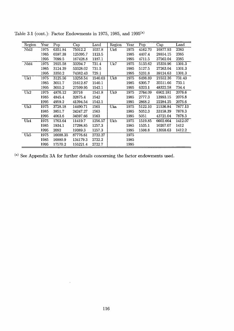
Table 3.1 (cont.): Factor Endowments in 1975, 1985, and 1995 )
Region Year Pop Cap Land Region Year Pop Cap LandNldS 1975 6351.84 75012.2 1037.8 Uk6 1975 4162.70 16877.93 2383
1985 6597.38 125395.7 1123.5 1985 4407.4 28854.15 23851995 7099.5 167428.8 1187.1 1995 4711.5 37562.04 2385
Nld4 1975 2925.58 33294.7 731.4 Uk7 1975 5133.62 15359.96 1301.31985 3124.39 53328.02 731.5 1985 5127.5 27263.04 1301.31995 3350.2 74382.43 729.1 1995 5231.8 39124.63 1301.3
Ukl 1975 3125.56 13258.54 1540.03 Uk8 1975 6498.89 21552.36 731.431985 3051.7 21612.87 1540.1 1985 6305.7 35511.66 733.11995 3055.2 27599.95 1542.1 1995 6323.1 48322.58 734.4
Uk2 1975 4876.12 20716 1541.8 Uk9 1975 2764.09 6902.181 2076.61985 4845.4 32875.4 1542 1985 2777.3 13993.15 2076.81995 4959.2 41394.54 1542.1 1995 2868.2 22284.25 2076.6
UkS 1975 3728.18 14490.71 1561 Uka 1975 5122.10 21536.84 7877.131985 3851.7 24247.27 1563 1985 5052.3 33158.39 7878.31995 4063.6 34597.66 1563 1995 5051 43721.04 7878.3
Uk4 1975 1763.64 11419.7 1256.57 Ukb 1975 1519.85 6602.664 1412.071985 1934.1 17298.85 1257.3 1985 1535.1 10267.07 14121995 2092 19389.3 1257.3 1995 1598.8 13058.63 1412.2
Uk5 1975 16688.35 87776.61 2722.27 19751985 16880.9 134179.3 2722.2 19851995 17570.2 155221.4 2722.7 1995
See Appendix 3A for further details concerning the factor endowments used.
116

Table 3.2: Educational Attainment by Region in 1985 and 1995 (percentage of total population)(a)
Region Year Low Med High Region Year Low Med HighBel 1985 5S.S5 41.55 5.10 Ita6 1985 60.43 29.38 9.41
1995 S5.97 59.68 4.35 1995 46.34 39.99 13.67Be2 1985 50.97 45.S5 3.67 Ita? 1985 71.65 21.99 6.30
1995 41.90 52.51 5.59 1995 56.26 34.15 9.59BeS 1985 51.07 45.27 3.66 ItaS 1985 73.40 19.98 6.71
1995 S7.49 57.20 5.31 1995 57.98 31.73 10.29Espl 1985 65.S1 28.52 6.18 Ita9 1985 73.91 20.45 5.72
1995 44.46 46.94 8.60 1995 60.67 29.67 9.67Esp2 1985 59.8S S2.45 7.72 Itaa 1985 70.94 21.73 7.26
1995 S8.S5 48.S0 13.34 1995 59.83 30.07 10.10EspS 1985 47.22 40.70 12.08 Itab 1985 77.40 17.16 5.79
1995 SS.51 50.17 16.32 1995 65.70 27.35 6.96Esp4 1985 67.42 26.44 6.14 Lux 1985 51.07 45.27 3.66
1995 48.11 42.4S 9.46 1990 37.49 57.20 5.31Esp5 1985 67.42 S0.49 6.13 Nidi 1985 29.75 62.33 9.03
1995 S9.S6 50.94 9.71 1995 14.86 68.53 16.79Esp6 1985 70.07 24.5S 5.39 Nld2 1985 27.76 62.77 9.33
1995 49.28 4S.28 7.45 1995 14.53 68.48 16.95Esp7 1985 65.S9 28.19 6.42 NldS 1985 28.33 58.68 12.02
1995 4S.66 46.2S 10.11 1995 14.80 62.88 22.12Fral 1985 46.1S S4.18 19.44 Nld4 1985 29.06 61.16 9.47
1994 S6.50 40.50 23.00 1995 15.08 67.58 17.08Fra2 1985 61.95 35.98 9.36 Ukl 1985 40.48 44.32 3.18
1994 40.00 38.50 21.50 1994 25.51 68.37 5.80FraS 1985 65.91 35.08 7.92 Uk2 1985 38.39 46.85 3.56
1994 49.00 38.50 12.50 1994 24.42 68.10 7.14Fra4 1985 55.S6 38.68 10.80 UkS 1985 34.89 47.15 4.43
1994 40.50 44.00 15.50 1994 24.81 67.38 7.60Fra5 1985 55.S6 38.68 10.08 Uk4 1985 36.31 48.60 4.66
1994 40.00 45.00 15.00 1994 21.79 70.63 7.49Fra6 1985 48.77 40.48 12.96 Uk5 1985 27.98 53.17 7.41
1994 S5.50 46.00 18.50 1994 19.44 68.50 11.71Fra? 1985 50.09 39.58 13.68 Uk6 1985 41.86 40.71 4.06
1994 S6.S2 44.28 19.40 1994 20.90 70.24 8.63FraS 1985 56.68 36.88 12.24 Uk7 1985 34.77 47.92 4.14
1994 41.79 41.29 16.92 1994 27.67 64.79 7.07Ital 1985 7S.54 21.43 5.06 UkS 1985 37.25 47.46 4.26
1995 56.55 34.64 8.81 1994 25.09 66.89 7.77Ita2 1985 74.0S 20.84 5.21 Uk9 1985 43.44 43.44 5.10
1995 54.46 35.32 10.22 1994 26.15 66.20 7.54ItaS 1985 77.29 18.46 4.54 Uka 1985 55.00 39.80 3.81
1995 56.92 35.54 7.54 1994 20.30 70.60 8.86Ita4 1985 71.98 22.00 5.97 Ukb 1985 55.62 39.18 3.97
1995 54.89 35.79 9.33 1994 35.40 56.13 8.05Ita5 1985
19957S.1956.84
21.3634.02
5.479.14
Notes: Figures may not sum to exactly 100 due to rounding. See Appendix 3A for further detailsconcerning the data used.
117
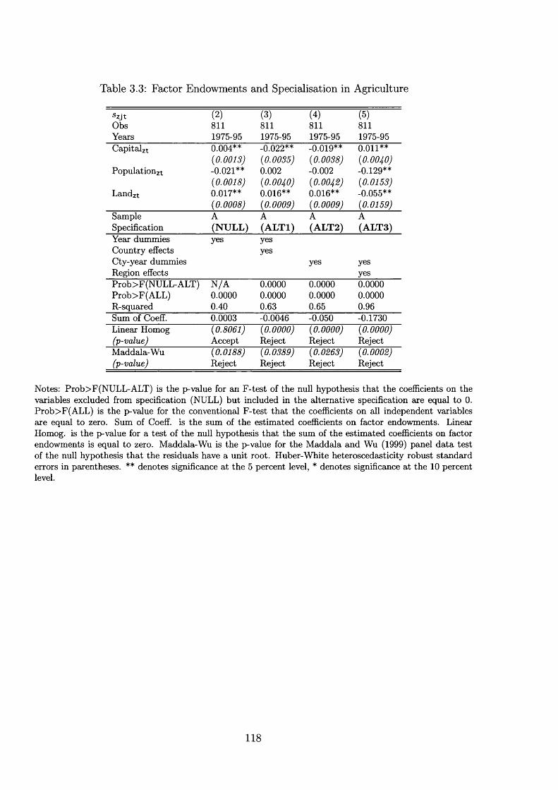
Table 3.3: Factor Endowments and Specialisation in Agriculture
5zjt (2) (3) (4) (5)Obs 811 811 811 811Years 1975-95 1975-95 1975-95 1975-95CapitaJzt 0.004** -0.022** -0.019** 0.011**
(0.001^; (0.000^; (o.oo^o;Populationzt -0.021** 0 . 0 0 2 -0.002 -0.129**
( 0 .0 0 1 ,9; (o.oo.^o;Landzt 0.017** 0.016** 0.016** -0.055**
{0.0008} (o.oooo; {0.0009} {0.0159}Sample A A A ASpecification (NU LL) (A L T l) (ALT2) (ALT3)Year dummies yes yesCountry effects yesCty-year dummies yes yesRegion effects yesProb>F(NULL-ALT) N /A 0.0000 0.0000 0.0000Prob>F(ALL) 0.0000 0.0000 0.0000 0.0000R-squared 0.40 0.63 0.65 0.96Sum of Coeff. 0.0003 -0.0046 -0.050 -0.1730Linear Homog {0.8061} {0.0000} {0.0000} {0.0000}(p-value) Accept Reject Reject RejectMaddala-Wu {0.0188} (o.o^gp; {0.0002}(p-value) Reject Reject Reject Reject
Notes: Prob>F(NULL-ALT) is the p-value for an F-test of the null hypothesis that the coefficients on the variables excluded from specification (NULL) but included in the alternative specification are equal to 0. Prob>F(ALL) is the p-value for the conventional F-test that the coefficients on all independent variables are equal to zero. Sum of Coeff. is the sum of the estimated coefficients on factor endowments. Linear Homog. is the p-value for a test of the null hypothesis that the sum of the estimated coefficients on factor endowments is equal to zero. Maddala-Wu is the p-value for the Maddala and Wu (1999) panel data test of the null hypothesis that the residuals have a unit root. Huber-White heteroscedasticity robust standard errors in parentheses. ** denotes significance at the 5 percent level, * denotes significance at the 10 percent level.
118

Table 3.4: Factor Endowments and Specialisation in Manufacturing
Szjt (2) (3) (4) (5)Obs 811 811 811 811Years 1975-95 1975-95 1975-95 1975-95Capitalzt -0.005 0.071** 0.073** 0.043**
(0.0116) (o.oloo; (o.ooog;Populationzt -0.008 -0.079** -0.082** 0.205**
(o.oojg; (o.oi.^o; (o.oo^g;Landzt 0.021** 0.032** 0.033** -0.130*
(0.00^^; (0.00^7) (o.oogo; (o.o7^p;Sample A A A ASpecification (N U LL) (A L T l) (ALT2) (ALT3)Year dummies yes yesCountry effects yesCty-year dummies yes yesRegion effects yesProb>F(NULL-ALT) N /A 0.0000 0.0000 0.0000Prob>F(ALL) 0.0000 0.0000 0.0000 0.0000R-squared 0.29 0.40 0.42 0.97Sum of Coeff. 0.0082 0.0239 0.0240 0.1180Linear Homog (0.0000) (0.0000)(p-value) Reject Reject Reject AcceptMaddala-Wu (o.oo^o; (0.00:90; (O.lOv O; (0.177P/(p-value) Reject Reject Accept Accept
Notes: Prob>F(NULL-ALT) is the p-value for an F-test of the null hypothesis that the coefficients on the variables excluded from specification (NULL) but included in the alternative specification are equal to 0. Prob>F(ALL) is the p-value for the conventional F-test that the coefficients on all independent variables are equal to zero. Sum of Coeff. is the sum of the estimated coefficients on factor endowments. Linear Homog. is the p-value for a test of the null hypothesis that the sum of the estimated coefficients on factor endowments is equal to zero. Maddala-Wu is the p-value for the Maddala and Wu (1999) panel data test of the null hypothesis that the residuals have a unit root. Huber-White heteroscedasticity robust standard errors in parentheses. ** denotes significance at the 5% level, * denotes significance at the 10% level.
119

Table 3.5; Factor Endowments and Specialisation in Services
■Szjt (2) (3) (4) (5)Obs 811 811 811 811Years 1975-95 1975-95 1975-95 1975-95Capitalzt 0.0006 -0.049** -0.054** -0.054**
(o.oo^p; (o.oR?o; (o .ou^ ;Populationzt 0.029** 0.078** 0.083** -0.076**
(0.00J7) {0.0106) {0.0119) (o.oggg;Landzt -0.038** -0.048** -0.048** 0.185**
(o.oogi; (0.00^5/ (O.OOgT) (o.og^g;Sample A A A ASpecification (N U LL) (A L T l) (ALT2) (ALT3)Year dummies yes yesCountry effects yesCty-year dummies yes yesRegion effects yesProb>F(NULL-ALT) N /A 0.0000 0.0000 0.0000Prob>F(ALL) 0.0000 0.0000 0.0000 0.0000R-squared 0.45 0.53 0.55 0.98Sum of Coeff. -0.0085 -0.0192 -0.019 0.055Linear Homog {0.0091) {0.0001) {0.0002)(p-value) Reject Reject Reject AcceptMaddala-Wu {0.1705) {0.4115)(p-value) Accept Accept Reject Accept
Notes: Prob>F(NULL-ALT) is the p-value for an F-test of the null hypothesis that the coefficients on the variables excluded from specification (NULL) but included in the alternative specification are equal to 0. Prob>F(ALL) is the p-value for the conventional F-test that the coefficients on all independent variables are equal to zero. Sum of Coeff. is the sum of the estimated coefficients on factor endowments. Linear Homog. is the p-value for a test of the null hypothesis that the sum of the estimated coefficients on factor endowments is equal to zero. Maddala-Wu is the p-value for the Maddala and Wu (1999) panel data test of the null hypothesis that the residuals have a unit root. Huber-White heteroscedasticity robust standard errors in parentheses. ** denotes significance at the 5% level, * denotes significance at the 10% level.
120
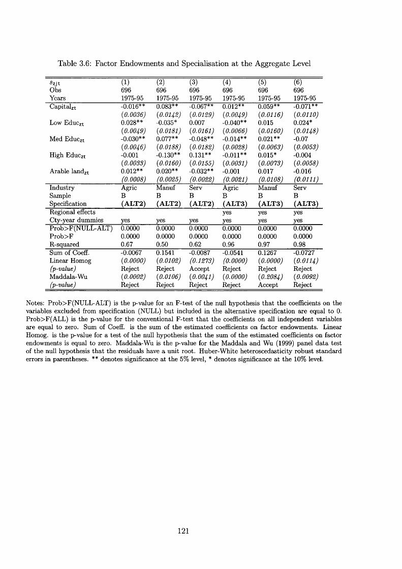
Table 3.6: Factor Endowments and Specialisation at the Aggregate Level
Szjt (1) (2) (3) (4) (5) (6)Obs 696 696 696 696 696 696Years 1975-95 1975-95 1975-95 1975-95 1975-95 1975-95Capitalzt -0.016** 0.083** -0.067** 0.012** 0.059** -0.071**
(o.oogg; (o.oigg; (o.oo.^p; (0.0116) (0.0110)Low Educzt 0.028** -0.035* 0.007 -0.040** 0.015 0.024*
(o.oo.^g; (o .o fg i; (0.0161) (o.oogg; (0.0160)Med EduCzt -0.030** 0.077** -0.048** -0.014** 0.021** -0.07
(0.0063) (0.0053)High Educzt -0.001 -0.130** 0.131** -0.011** 0.015* -0.004
(0.0033) (0.0160) (0.0155) (0.0031) (0.0073) (0.0058)Arable landzt 0.012** 0.020** -0.032** -0.001 0.017 -0.016
(0.0008) (0.0021) (0.0108) (0.0111)Industry Agric Manuf Serv Agric Manuf ServSample B B B B B BSpecification (ALT2) (ALT2) (ALT2) (ALT3) (ALT3) (ALT3)Regional effects yes yes yesCty-year dummies yes yes yes yes yes yesProb>F(NULL-ALT) 0.0000 0.0000 0.0000 0.0000 0.0000 0.0000Prob>F 0.0000 0.0000 0.0000 0.0000 0.0000 0.0000R-squared 0.67 0.50 0.62 0.96 0.97 0.98Sum of Coeff. -0.0067 0.1541 -0.0087 -0.0541 0.1267 -0.0727Linear Homog (0.0000) (0.0102) (0.0000) (0.0000) (0.0114)(p-value) Reject Reject Accept Reject Reject RejectMaddala-Wu (o.ooog; (0.0106) (0.0041) (0.0000) (o.gog^; (0.0092)(p-value) Reject Reject Reject Reject Accept Reject
Notes: Prob>F(NULL-ALT) is the p-value for an F-test of the null hypothesis that the coefficients on the variables excluded from specification (NULL) but included in the alternative specification are equal to 0. Prob>F(ALL) is the p-value for the conventional F-test that the coefficients on all independent variables are equal to zero. Sum of Coeff. is the sum of the estimated coefficients on factor endowments. Linear Homog. is the p-value for a test of the null hypothesis that the sum of the estimated coefficients on factor endowments is equal to zero. Maddala-Wu is the p-value for the Maddala and Wu (1999) panel data test of the null hypothesis that the residuals have a unit root. Huber-White heteroscedasticity robust standard errors in parentheses. ** denotes significance at the 5% level, * denotes significance at the 10% level.
121

Table 3.7: Factor Endowments and Specialisation at the Aggregate Level (Long Differences)
Aszjt (1) (2) (3)Obs 341 341 341
Years 1975-95 1975-95 1975-95A Capitalzt -0.006 0.062** -0.057**
ALow Educzt -0.035** -0.009 0.044**
AMed EduCzt -0.031** 0.023** 0.008{0.0081}
AHigh EduCzt -0.010** -0.002 0.012**{0.0017}
A Arable Landzt 0.013** 0.018* -0.031**{0.0108} (o.oigjg;
Industry Agric Manuf ServSample B B B
Specification (ALT4) (ALT4) (ALT4)Year dummies yes yes yes
Difference period 10 years 10 years 10 yearsProb>F 0.0000 0.0000 0.0000
R-squared 0.46 0.21 0.19Sum of Coeff. -0.0685 0.0915 -0.0229Linear Homog {0.0000} {0.0016}
(p-value) Reject Reject Accept
Notes: Sum of Coeff. is the sum of the estimated coefficients on factor endowments. Linear Homog. is the p-value for a test of the null hypothesis that the sum of the estimated coefficients on factor endowments is equal to zero. Huber-White heteroscedasticity robust standard errors in parentheses. ** denotes significance at the 5% level, * denotes significance at the 10% level.
122

Table 3.8: Average Shares of Sectors in GDP and Within-sample Average Absolute Prediction Errors
(1) (2) (3)Agric Manuf Serv
All countries^ GDP share 0.042 0.354 0.604Prediction Error 1 ALT2) 0.582 0.133 0.068Prediction Error 2 ALT2 on ly cty-yr) 6.316 0.499 0.159Prediction Error 3 ALT2 on ly endow .) 6.985 0.501 1.099
Belgium(^) GDP shaxe 0.026 0.337 0.637Prediction Error 1 ALT2) 0.519 0.056 0.038Prediction Error 2 ALT2 on ly cty-yr) 5.151 0.572 0.107Prediction Error 3 ALT2 on ly endow .) 5.632 0.476 1.099
Spain GDP share 0.057 0.334 0.609Prediction Error 1 ALT2) 1.529 0.170 0.072Prediction Error 2 ALT2 on ly cty-yr) 10.603 0.439 0.159Prediction Error 3 ALT2 on ly endow .) 10.277 0.524 1.095
Prance GDP share 0.043 0.337 0.620Prediction Error 1 ALT2) 0.677 0.118 0.046Prediction Error 2 ALT2 on ly cty-yr) 8.700 0.526 0.124Prediction Error 3 ALT2 on ly endow .) 9.267 0.461 1.104
Italy GDP share 0.048 0.339 0.613Prediction Error 1 ALT2) 0.280 0.121 0.053Prediction Error 2 ALT2 on ly cty-yr) 2.940 0.502 0.151Prediction Error 3 ALT2 on ly endow .) 3.822 0.471 1.133
Luxembourg GDP share 0.024 0.342 0.634Prediction Error 1 ALT2) 0(c) 0(c) 0(c)Prediction Error 2 ALT2 only cty-yr) 5.003 0.897 0.301Prediction Error 3 ALT2 on ly endow .) 6.003 0.104 1.301
Netherlands GDP share 0.047 0.353 0.600Prediction Error 1 ALT2) 0.125 0.177 0.114Prediction Error 2 ALT2 on ly cty-yr) 3.875 0.526 0.156Prediction Error 3 ALT2 on ly endow .) 4.858 0.426 1.058
UK GDP share 0.025 0.415 0.561Prediction Error 1 ALT2) 0.462 0.145 0.098Prediction Error 2 ALT2 on ly cty-yr) 6.634 0.444 0.213Prediction Error 3 ALT2 on ly endow .) 7.755 0.650 1.057Sample B B B
Notes: Table reports mean values for the whole sample and individual countries. Absolute proportional prediction errors are calculated as |s - s(P)| / s, where a capital P indicates a predicted value. Prediction error (ALT2) is based on the fitted values from specification (ALT2) using the disaggregated data on 5 factor endowments, and parameter estimates for this specification are reported in Table 3.5; Prediction error (ALT2, only cty-year) indicates that predicted values use the parameter estimates from specification (ALT2) but only the country-year dummies are used to construct predicted shares of GDP. Prediction error (ALT2, only endowments) indicates that predicted values use the parameter estimates from specification (ALT2) but only the 5 factor endowments are used to construct predicted shares of GDP.
Reported prediction errors exclude region B el (Brussels). Brussels is a capital city, and the share of Agriculture in this region is a clear outlier. As a robustness test, we re-estimated the model excluding this region; this produced very similar estimated coefficients to those reported earlier, (b) Luxembourg has only one NUTS-1 region. The fitted values for shares of sectors in GDP in the specification with country-year dummies are therefore exactly equal to the actual values (we estimate as many country-year coefficients as there are observations for Luxembourg). We experimented with treating Luxembourg as a region of Belgium; again this yielded very similar estimated coefficients to those reported earlier.
123

Table 3.9: Within-sample Average Absolute Prediction Errors over Time
Period (1) (2) (3)All countries(^) Prediction Error (ALT2) 1980-85 0.568 0.132 0.070
Prediction Error (ALT2) 1985-90 0.735 0.130 0.062Prediction Error (ALT2) 1990-95 0.566 0.131 0.054
Belgium(^) Prediction Error (ALT2) 1980-85 0.403 0.031 0.029Prediction Error (ALT2) 1985-90 0.421 0.064 0.040Prediction Error (ALT2) 1990-95 0.708 0.078 0.048
Spain Prediction Error (ALT2) 1980-85 1.195 0.191 0.083Prediction Error (ALT2) 1985-90 1.983 0.157 0.068Prediction Error (ALT2) 1990-95 1.513 0.164 0.064
France Prediction Error (ALT2) 1980-85 0.724 0.111 0.042Prediction Error (ALT2) 1985-90 0.721 0.126 0.043Prediction Error (ALT2) 1990-94 0.565 0.117 0.043
Italy Prediction Error (ALT2) 1980-85 0.340 0.107 0.047Prediction Error (ALT2) 1985-90 0.283 0.126 0.059Prediction Error (ALT2) 1990-95 0.213 0.129 0.053
Luxembourg Prediction Error (ALT2) 1980-85 0(b) 0(b) 0(b)Prediction Error (ALT2) 1985-90 0(b) 0(b) 0(b)
Netherlands Prediction Error (ALT2) 1980-85 0.174 0.224 0.170Prediction Error (ALT2) 1985-90 0.114 0.172 0.103Prediction Error (ALT2) 1990-95 0.083 0.141 0.065
UK Prediction Error (ALT2) 1975-80 0.328 0.165 0.117Prediction Error (ALT2) 1980-85 0.501 0.129 0.082Sample B B B
Notes: Table reports mean values for the whole sample and individual countries. Absolute proportional prediction errors are calculated as |s - s(P)| / s, where a capital P indicates a predicted value. Prediction error (ALT2) is based on the fitted values from specification (ALT2) using the disaggregated data on 5 factor endowments, and parameter estimates for this specification are reported in Table 3.6. (a) Reported prediction errors exclude region Bel (Brussels). Brussels is a capital city, and the share of Agriculture in this region is a clear outlier. As a robustness test, we re-estimated the model excluding this region; this produced very similar estimated coefficients to those reported earlier, (b) Luxembourg has only one NUTS-1 region. The fitted values for shares of sectors in GDP in the specification with country-year dummies are therefore exactly equal to the actual values (we estimate as many country-year coefficients as there are observations for Luxembourg). We experimented with treating Luxembourg as a region of Belgium; again this yielded very similar estimated coefficients to those reported earlier.
124

Table 3.10: Within-sample Average Absolute Prediction Errors (PE (ALT2)) in the Disaggregated Manufacturing Industries over Time
(1) (2) (3) (4) (5) (6)C ountry P eriod Fuel Ferrous M inerals Chem ical M achine TransportAll countries(^)'(^) 1980-85 0.579 2.467 0.286 0.457 0.486 0.575
1985-90 0.542 1.455 0.279 0.350 0.496 0.5121990-95 0.536 1.246 0.286 0.389 0.551 0.550
Belgium(^^ 1980-85 0.402 0.357 0.583 0.252 0.266 1.0111985-90 0.271 0.246 0.542 0.213 0.167 0.1561990-95 0.123 0.320 0.480 0.209 0.193 0.136
Spain(b) 1980-85 0.569 1.953 0.211 0.741 1.235 1.2171985-90 0.378 2.289 0.259 0.497 1.155 0.6491990-94 0.339 1.958 0.274 0.548 1.247 0.833
Prance 1980-85 0.325 0.886 0.216 0.318 0.283 0.2881985-90 0.341 0.922 0.209 0.339 0.259 0.3711990-94 0.421 1.146 0.175 0.342 0.274 0.371
Italy 1980-85 0.396 1.263 0.289 0.330 0.488 0.6051985-90 0.399 1.218 0.271 0.307 0.415 0.7141990-95 0.378 1.215 0.282 0.435 0.483 0.634
Luxembourg 1980-85 0(U 0(U 0(c) 0(c) 0(c) 0(c)1985-90 0(U 0 (c) 0 (c) 0 (c) 0(c) 0 (c)
Netherlands 1980-85 1.442 0.473 0.363 0.330 0.439 0.3661985-90 1.561 0.420 0.392 0.213 0.415 0.4281990-95 1.578 0.789 0.414 0.198 0.388 0.436
UK 1975-80 0.654 3.720 0.529 0.548 0.319 0.4921980-85 0.722 6.731 0.324 0.579 0.257 0.395Sample B B B B B B
Notes: Table reports mean values for the whole sample and individual countries. For full industry names, see Appendix A. Absolute proportional prediction errors are calculated as |s - s(P)| / s, where a capital P indicates a predicted value. Prediction error (ALT2) is based on the fitted values from specification (ALT2) using the disaggregated data on 5 factor endowments, and parameter estimates for this specification are reported in Table 3.6. (a) The reported prediction errors exclude region Bel (Brussels). Brussels is a capital city, and the shares of some disaggregated manufacturing industries in this region are clear outliers. As a robustness test, we re-estimated the model excluding this region; this produced very similar estimated coefficients to those reported earlier.
125

Table 3.11: Within-sample Average Absolute Prediction Errors (PE (ALT2)) in the Disaggregated Manufacturing Industries over Time
(1) (2) (3) (4) (5)C ountry P eriod Food T extile P aper O ther C onstructionAll countries 1980-85 0.239 0.784 0.296 0.334 0.127
1985-90 0.240 0.730 0.395 0.351 0.1251990-95 0.242 0.813 0.469 0.390 0.093
Belgium(^) 1980-85 0.288 0.189 0.331 0.374 0.0641985-90 0.245 0.249 0.256 0.217 0.0751990-95 0.324 0.174 0.292 0.171 0.022
Spain(b) 1980-85 0.198 1.050 0.402 0.454 0.1341985-90 0.185 0.756 0.490 0.539 0.1331990-95 0.152 0.916 0.552 0.586 0.112
France 1980-85 0.146 0.476 0.195 0.314 0.0891985-90 0.115 0.499 0.196 0.346 0.0681990-94 0.142 0.489 0.229 0.403 0.063
Italy 1980-85 0.252 0.628 0.481 0.328 0.1991985-90 0.283 0.801 0.698 0.294 0.1791990-95 0.345 1.065 0.723 0.341 0.104
Luxembourg 1980-85 0(c) 0(c) 0(c) 0(c) 0(c)1985-90 0(c) 0(c) 0(c) 0 (c) 0 (c)
Netherlands 1980-85 0.213 1.691 0.147 0.427 0.1091985-90 0.324 1.279 0.153 0.370 0.1381990-95 0.225 0.862 0.157 0.340 0.126
UK 1975-80 0.418 1.111 0.282 0.264 0.0831980-85 0.345 0.845 0.191 0.269 0.110Sample B B B B B
Notes: Table reports mean values for the whole sample and individual countries. For full industry names, see Appendix 3A. Absolute proportional prediction errors are calculated as |s - s(P)| / s, where a capital P indicates a predicted value. Prediction error (ALT2) is based on the fitted values from specification (ALT2) using the disaggregated data on 5 factor endowments, and parameter estimates for this specification are reported in Table 3.6. (a) The reported prediction errors exclude region Bel (Brussels). Brussels is a capital city, and the shares of some disaggregated manufacturing industries in this region are clear outliers. As a robustness test, we re-estimated the model excluding this region; this produced very similar estimated coefficients to those reported earlier.
126
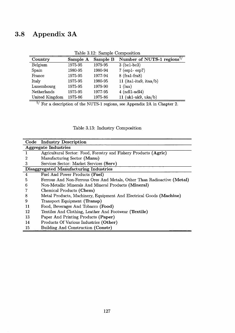
3.8 Appendix SA
Table 3.12: Sample CompositionCountry Sample A Scunple B N um ber of NUTS-1 regions^/Belgium 1975-95 1979-95 3 (bel-be3)Spain 1980-95 1980-94 7 (espl- esp7)France 1975-95 1977-94 8 (fral-fra8)Italy 1975-95 1980-95 11 (ital-ita9, itaa/b)Luxembourg 1975-95 1979-90 1 (lux)Netherlands 1975-95 1977-95 4 (ndll-ndl4)United Kingdom 1975-86 1975-86 11 (ukl-uk9, uka/b)
For a description of the NUTS-1 regions, see Appendix 2A in Chapter 2.
Table 3.13: Industry Composition
Code Industry DescriptionAggregate Industries1 Agricultural Sector: Food, Forestry and Fishery Products (Agric)2 Manufacturing Sector (Manu)3 Services Sector: Market Services (Serv)Disaggregated M anufacturing Industries4 Fuel And Power Products (Fuel)5 Ferrous And Non-Ferrous Ores And Metals, Other Than Radioactive (M etal)6 Non-Metallic Minerals And Mineral Products (Mineral)7 Chemical Products (Chem)8 Metal Products, Machinery, Equipment And Electrical Goods (Machine)9 Transport Equipment (Transp)11 Food, Beverages And Tobacco (Food)12 Textiles And Clothing, Leather And Footwear (Textile)13 Paper And Printing Products (Paper)14 Products Of Various Industries (O ther)15 Building And Construction (Constr)
127

3.9 Appendix 3B
3.9 .1 B l . R eg ion a l-leve l D a ta on P ro d u ctio n and E n d ow m en ts
1. Value Added: current price value-added, millions of ECUs, from Regio dataset, Eurostat.
2. GDP: current price, millions of ECUs, from Regio dataset, Eurostat.
3. Population: total population, thousands of people, from Regio dataset, Eurostat.
4. Land: total land area, thousands of hectares, from Regio dataset, Eurostat.
5. Arable Land: total arable land area, thousands of hectares, from Regio dataset, Eurostat.
6. Capital Stock: constructed by the perpetual inventory method (see, for example, Barro
and Sala-i-Martin, 1995) using regional-level investment data (Gross Fixed Capital Formation),
constant 1990 prices, millions of ECUs. The main source for the investment data is the Regio
dataset, Eurostat. Current price investment was converted into constant prices using price deflators
from the Penn World Tables, 5.6. For some countries, regional current price investment data were
extended backwards in time using country-level information from the IMF International Financial
Statistics.
B 2. Sum m ary o f E d u cation a l A tta in m en t D a ta S ources
Following the labour market literature (see, for example, Nickell and Bell, 1996, and Machin and
Van Reenen, 1998), educational attainment is grouped into three categories: low, medium and high.
‘Low education’ is no or primary education, while ‘high education’ is College degree or equivalent.
‘Medium education’ corresponds to all intermediate levels of educational attainment, including
secondary school and vocational qualifications. Using individual country labour force surveys,
we compute the percentage of the population with each level of educational attainment. The
endowment variables included in the regressions are these percentages multiplied by the population
data from Regio, Eurostat.
1. Belgium: regional data on educational attainment from Annuaire de Statistiques Régionales.
Years available are 1970, 1977, 1981 and 1991. Linear interpolation of the data.
2. Spain: educational attainment data from Spanish Labour Force, Institute Nacional de Estadis-
tica. Years available are 1977, 1979, 1981, and 1983-94. Linear interpolation of the data when
required.
3. Italy: educational attainment data from 1986-97 is from Forze di Lavoro and Rilevazione delle
foTze di Lavore, ISTAT. For years prior to 1986, the regional data is extended backwards in time
128

using country-level information from Nickell et al. (2000).
4. France: educational attainment data from Key data on Education, DG for Education and
Culture, European Commission. Years available are 1993 and 1995. Linear interpolation of the
data for 1994. The regional data are extended backwards in time country-level information from
Nickell et al. (2000).
5. N etherlands: Data from National Statistical Office, years 1992-98. The regional data are
extended backwards in time using country-level information from Nickell et al. (2000).
6. Luxembourg: Data are from Belgian region closest to Luxembourg (beS, Region Wallone).
7. U nited Kingdom: Data from the Labour Force Survey, years 1977, 1979, 1981, and 1983-94.
Linear interpolation of the data when required. Bibliographic citation: Office for National Statistics
Labour Market Statistics Croup, Department of Finance and Personnel (Northern Ireland), Central
Survey Unit, Quarterly Labour Force Survey. Data distributed by the Data Archive, Colchester,
Essex. Data disclaimer: although all efforts are made to ensure the quality of the materials, neither
the copyright holder, the original data producer, the relevant funding agency. The Data Archive,
bear any responsibility for the accuracy or comprehensiveness of these materials.
129

3.10 Appendix 3C
Table 3.14: Factor Endowments and Specialisation at the Disaggregate LevelGDP share (1) (2) (3) (4) (5) (6)Obs 696 689 689 696 696 693Years 1975-95 1975-95 1975-95 1975-95 1975-95 1975-95Capital 0.006 -0.008** -0.001 0.007** 0.036** 0.001
("o.oogp; (0.0017) ("g.gggg; ("g.007. ; ("g.gg. 7) ("g.gggg;Low Educ -0.035** 0.009** 0.002** -0.001 -0.017** 0.004**
(0.0015) ("g.ggg?; (0.0030) (0.0011)Med Educ 0.001 0.004 -0.002** 0.005** 0.038** 0.010***
(0.0056) ("g.gggg; (0.0008) (0.0019) (0.0056) (0.0021)High Educ -0.001 -0.004** -0.003** -0.004** -0.040** -0.008**
(0.0050) (0.0017) ("g.gggg; (0.0018) (0.0020)Arable Land 0.010** 0.001** 0.003** -0.001 -0.001 -0.001**
(0.0016) (0.0004) (0.0004) (0.0007) (0.0003)Industry Fuel Metal Mineral Chem Machine TranspSample B B B B B BSpecification (ALT2) (ALT2) (ALT2) (ALT2) (ALT2) (ALT2)Cty-year dummies yes yes yes yes yes yesProb>F(NULL-ALT2) XXX XXX XXX XXX XXX XXXProb>F(ALL) 0.0000 0.0000 0.0000 0.0000 0.0000 0.0000R-squared 0.25 0.64 0.47 0.31 0.35 0.34Sum of Coeff. 0.0710 0.0020 -0.0010 0.0060 0.0160 0.0060Linear Homog (0.0000) (0.0016) ("g.gjgg; (0.0000) (0.0000) (0.0000)(p-value) Accept Accept Accept Accept Accept AcceptMaddala-Wu(p-value)
Notes; for full industry names, see Appendix A. Prob>F(NULL-ALT) is the p-value for an F-test of the null hypothesis that the coefficients on the variables excluded from specification (NULL) but included in the alternative specification are equal to 0. Prob>F(ALL) is the p-value for the conventional F-test that the coefficients on all independent variables are equal to zero. Sum of Coeff. is the sum of the estimated coefficients on factor endowments. Linear Homog. is the p-value for a test of the null hypothesis that the sum of the estimated coefficients on factor endowments is equal to zero. Maddala-Wu is the p-value for the Maddala and Wu (1999) panel data test of the null hypothesis that the residuals have a unit root. Huber-White heteroscedasticity robust standard errors in parentheses. ** denotes significance at the 5% level, * denotes significance at the 10% level.
130

Table 3.15: Factor Endowments and Specialisation at the Disaggregate Level
GDP share (1) (2) (3) (4) (5)Obs 696 696 696 696 696Years 1975-95 1975-95 1975-95 1975-95 1975-95Capital 0.013*** 0.021*** 0.008*** 0.014*** -0.010***
("0.00.01; ("0.000 ; ("0.000, ; ("o.oof. ; (0.0017)Low Educ -0.003* 0.008*** -0.008*** 0.003*** 0.005***
("o.oof?; (0.0015) (0.0005) ("o.oooo; ("0.0010;Med Educ 0.001 0.008*** 0.009*** 0.005*** -0.021***
("o.oooo; ("0.000?; ("o.oofo; ("O.OO0 O;High Educ -0.022*** -0.029*** -0.005*** -0.017*** 0.013***
("O.OO;0O; ("O.OO0 O; (0.0008) (0.0014) (0.0019)Arable Land 0.004*** 0.001*** -0.001*** 0.002*** 0.005***
(0.0005) (0.0004) ("0.0000; (0.0002) (0.0004)Industry Food Textile Paper Other ConstructionSample B B B B BSpecification (ALT2) (ALT2) (ALT2) (ALT2) (ALT2)Cty-year dummies yes yes yes yes yesProb>F(NULL-ALT2) XXX XXX XXX XXX XXXProb>F(ALL) 0.0000 0.0000 0.0000 0.0000 0.0000R-squared 0.54 0.42 0.56 0.47 0.64Sum of Coeff. -0.0070 0.0090 0.0030 0.0070 -0.0080Linear Homog (0.0001) (0.0000) (0.0000) (0.0000) (0.0000)(p-value) Accept Accept Accept Accept AcceptMaddala-Wu(p-value)
Notes: for full industry names, see Appendix A. Prob>F(NULL-ALT) is the p-value for an F-test of the null hypothesis that the coefficients on the variables excluded from specification (NULL) but included in the alternative specification are equal to 0. Prob>F(ALL) is the p-value for the conventional F-test that the coefficients on all independent variables are equal to zero. Sum of Coeff. is the sum of the estimated coefficients on factor endowments. Linear Homog. is the p-value for a test of the null hypothesis that the sum of the estimated coefficients on factor endowments is equal to zero. Maddala-Wu is the p-value for the Maddala and Wu (1999) panel data test of the null hypothesis that the residuals have a unit root. Huber-White heteroscedasticity robust standard errors in parentheses. ** denotes significance at the 5% level, * denotes significance at the 10% level.
131

Chapter 4
Factor Endowm ents, Econom ic
Geography, and Specialisation in
European Regions
4.1 Introduction
In the two previous chapters, we analysed the evolution of specialisation in European regions and
countries, and the role of factor endowments in determining the pattern of production in European
regions. In particular, Chapter 3 considered the neoclassical model of trade of which the Heckscher-
Ohlin model is a special case. Under the assumptions of the Heckscher-Ohlin model, we derived
an equation relating specialisation (measured as the share of an industry’s value-added in GDP) to
relative prices and factor endowments. Across a wide range of econometric specifications, there is a
statistically significant and quantitatively important relationship between factor endowments and
patterns of production. Factor endowments are most successful in explaining production patterns
at the aggregate level. In particular, among the 3 aggregate industries considered, factor endow
ments are most successful at explaining regional specialisation in Services and Manufacturing. We
found no evidence that the process of increasing economic integration in Europe has weakened the
relationship between patterns of production and factor endowments within countries over time.
While the Neoclassical model was reasonably successful in explaining patterns of production at
the aggregate level, the econometric specifications were less successful in explaining specialisation
within manufacturing industries. In this case, the average prediction error across regions from
1985-90 was 47 percent, compared with an average prediction error across the three aggregated
132

industries of 31 percent during the same period. As set forth in the last chapter, one theory-
consistent explanation for the larger prediction errors for disaggregated industries is indeterminacy
in the production of individual manufacturing industries at the regional level. Another explanation
is that the analysis in Chapter 3 neglected economic geography considerations. A large theoretical
literature has emphasised the role of transport costs and increasing returns to scale in determining
the location of production. Given the size of the prediction errors, we could expect that economic
geography effects operate most strongly in disaggregated manufacturing industries. Intuitively,
increasing returns to scale imply that firms would like to concentrate in a single location, while
the existence of transport costs implies that, other things equal, this concentration will occur close
to large markets and sources of supply. Other things being equal, industries will locate in regions
with good market access and sources of supply of intermediate goods.
Economic geography models incorporate the role of location of agents relative to one another
in physical space into the analysis. The model may have multiple equilibria, some unstable, and
other with agglomeration (see for example, Krugman, 1991a and 1991b). If trade is perfectly
free (no transport cost), comparative advantage (as driven by technology and factor endowments)
determines the structure of production in each region. However, if transport costs are also present
in the analysis, then both supply and demand matters for the location of economic activity, and
industries would want to be relatively close to suppliers and consumers (benefiting from backward
and forward linkages). These linkages are important in creating and sustaining spatial concentration
of economic activity, as firms exploit their economies of scale. If transport costs depend on distance,
then geographical factors play a role determining the location of production in each region. In
practice, both factor endowments and economic geography are important. Moreover, given the
process of integration that has taken place in Europe since the Second World War, there are reasons
for thinking that economic geography may have a particularly important role to play in Europe.
This chapter reviews a general theoretical model that incorporates both sets of considerations before
presenting empirical evidence on the relative importance of each using European regional data.
The analysis is the first of its kind using European regional data. We extend the analysis of the
previous chapter by incorporating considerations of economic geography alongside those of factor
endowments and factor intensities to explain specialisation at the regional level in Europe, in line
with the approach developed by Midelfart-Knarvik et al. (2000b). We derive an equation relating an
industry’s value-added share in GDP to factor endowments and the location of supply and demand,
factors determining the location of production in conjunction with industry characteristics, such as
factor intensities and transport costs. We focus on the manufacturing industries, els the analysis in
the previous chapter found the largest prediction errors in disaggregated manufacturing.
133
We find that both factor endowments and economic geography are relevant forces in explaining
specialisation in the manufacturing sector across European regions. Parameter estimates are sta
tistically significant and constant across different specifications that account for different sources of
unobserved heterogeneity in the data. Other things being equal, regions with high skill endowments
would be more specialised in skill-intensive industries. Among the economic geography variables,
the interaction term of access to suppliers and intermediate demand intensity is always statisti
cally significant in explaining specialisation at the one percent level. Regions with good access
to intermediate goods attract industries using intermediate goods more intensively, and become
more specialised in those industries over time. Location with respect to supply is more relevant for
specialisation than the location of demand.
Our model performs well in explaining patterns of specialisation across European regions. The
model’s average prediction error across all disaggregated manufacturing industries, regions, and
time is 13 percent, and ranges from 8 percent to 20 percent in individual manufacturing industries.
Hence, average prediction errors compare positively with those reported in Chapter 3. The average
prediction error for the eight manufacturing industries was 58 percent during 1985-95 when con
sidering only the role of factor endowments. Furthermore, when using the estimated coefficients to
evaluate predicted shares of GDP excluding information on factor endowments, economic geogra
phy and industry characteristics; the average prediction error in manufacturing industries across
all countries, industries, and years rises to 120 percent. Over time, prediction errors remain stable,
not only across countries, but also across industries in our sample.
4.2 Related Literature
Although this chapter relates to the empirical literature on both the role of factor endowments and
the role of economic geography in determining the location of production, this section focuses on
the existing empirical work in economic geography.^ A large theoretical literature has emphasised
the role of transport costs and increasing returns to scale in determining the location of production
(see Fujita, Krugman, and Venables, 1999). Increasing returns to scale imply that firms would
like to concentrate production in a single location, while the existence of transport costs implies
that, other things equal, this concentration will occur close to large markets and sources of supply.
The geographical structure of trade costs mean that some locations will be attractive to industry
because of good market access and also because of good intermediate supplier access.
^For a review of the recent empirical literature on the role of factor endowments, see Section 3.2 on related literature in Chapter 3.
134

Based on this theoretical literature, a number of studies have described how specialisation and
concentration have evolved, as reviewed in Chapter 2. A smaller number of studies have analysed
the underlying economic determinants of the location of activity. The studies find support for
the new trade theories and economic geography models. In general, two related dimensions are
considered in these studies; how localised a certain economic activity is, and how specialised a
certain geographical unit is. A series of studies find evidence of increasing localisation and special
isation within countries or a group of countries. Kim (1995) found evidence of a non-monotonic
evolution of specialisation and localisation across the states within the United States during the
period 1860-1987. States became more specialised until 1930, when the process was reversed —
specialisation is lower today that it was in 1860. In the European Union, these kind of studies have
found increasing specialisation and localisation as European integration proceeds. Amiti (1999)
and Midelfart-Knarvik et al. (2000a) both found increasing specialisation across European coun
tries from the mid-1980 onwards, the first study using data on employment and production and the
second, using data on gross output. However, although these studies describe well the evolution
of specialisation and localisation, they devote relatively little attention to determining the under
lying forces of the process. Evidence of increasing specialisation and localisation by itself does not
discriminate between comparative advantage and economic geography.
Consequently, a number of studies in the literature have tried to identify the underlying forces
shaping specialisation and localisation. Two different approaches have been adopted at the inter
national level. One approach has tried to identify home market effects, or an increase in demand
for a good reflects in a more than proportionate increase in production of the good. Davis and
Weinstein (1998, 2003) use this home market effect for testing between models of imperfect com
petition/increasing returns to scale and perfect competition/ constant return to scale. Davis and
Weinstein (1998) consider a nested specification where factor endowments are assumed to determine
production at the three-digit industry level, while economic geography effects operate in disaggre
gated industries. Using data for 13 OECD countries, they first construct measures of idiosyncratic
demand for each four-digit industry based on demand in the country and its trading partners.
Estimating the impact of this demand variable on production in a pooled sample across countries
and all four-digit industries, they find evidence of a strong home market effect. Disaggregating and
running separate regressions for each three-digit industry with a sample of countries and four-digit
sub-industries, they also find evidence of a home market effect in a majority of industries. Head and
Ries (2001) find a weak home market effect when looking at the United States and Canada trade at
the three-digit level during the period 1990-95. Feenstra, Markusen and Rose (2001) identify a home
market effect in estimating a gravity model separately for differentiated products, reference-priced
135

exports, and homogeneous goods. Another approach tries to combine comparative advantage and
economic geography to investigate the relative contribution of the forces underlying localisation
and specialisation. Midelfart-Knarvik et al. (2000b) develop a model where both elements explain
the location of production in Europe. They find endowments of skilled and scientific labour as
well as forward and backward linkages to be important determinants of industrial structure over
the sample period 1980-92 at the country level. Also, economic geography effects are becoming
econometrically more relevant over time, which could be attributable to the process of economic
integration.
At the subnational level, the empirical literature addresses issues such as of the existence and
determination of clustering. Hanson (1998) examines the spatial distribution of economic activity
within the United States, and finds significant demand linkages across regions. Estimating the
structural parameters of the Krugman (1991a) model of economic geography, he finds small but
significant scale economies. Geographic concentration is found to be a stable feature of the spatial
distribution of economic activity. Demand linkages are strong across regions and are growing
over time, although limited in geographic scope. Davis and Weinstein (1999), in a specification
similar to the study mentioned above, find significant home market effects when considering 29
sectors and 47 Japanese perfectures in 1985. These effects are quantitatively important: for the
eight sectors with statistically significant home market effects, a one standard deviation movement
in idiosyncratic demand is found to move production by half a standard deviation on average.
Ellison and Glaeser (1999) consider the extent at which localisation can be explained by natural
advantage, studying the shares of U.S. states in different industries as a function of the interaction
between industry and state characteristics. Their results suggest that between 50 percent and 80
percent of localisation at the state level is left unexplained by natural advantage. Different lines of
research have tried to explain this residual excess localisation, either by assessing the importance of
localisation versus urbanisation economies (see Henderson, 1999 for a discussion of these issues), or
by analysing the effect of the scale or density of economic activity on productivity levels (Ciccone
and Hall, 1996, and Davis and Weinstein, 2001). However, these subnational studies have focused
on determining either the role of comparative advantage or of economic geography in the pattern
of localisation/ specialisation independently.^ None of the studies are done at the subnational
European level, which represents an interesting context given the process of economic integration
during the post-war period.
This chapter analyses how economic geography and factor endowments jointly determine the
^Duranton and Overman (2001) looks within the U.K. using microgeographic data.
136
pattern of specialisation in European regions. The analysis builds on a theoretical background
that integrates both factor endowments and economic geography considerations. The study is the
first of its kind using regional data in Europe. We consider a measure of specialisation derived
from theory and consistent with the measure used in the previous chapter—the GDP share of
industry j in region z. In describing the model, we are able to establish a relationship between the
share of an industry’s value added in GDP, factor endowunents, and economic geography variables.
We concentrate on industries within the manufacturing sector across 45 European regions. The
model estimated here is broader than the one used in the previous chapter, as we explicitly analyse
both factor endowments/ industry intensities and economic geography factors in the location of
production in European regions.
The rest of the chapter is structured as follows. Section 3 outlines the model and the equation
relating our measure of specialisation to factor endowments and economic geography variables. Sec
tion 4 describes the data. Section 5 discusses the econometric estimation, and Section 6 concludes.
4.3 The model
In this section, we outline a canonical model relating economic geography factors to the structure
of production. We follow Midelfart-Knarvik et al. (2000b) and Overman, Redding and Venables
(2001). The model considers a number of regions (locations) despicted by the subscript z and a
number of industries, indexed by j. Denote jzjt as the level of production in region z of industry
j at time The demand side of the model takes a CES form, with the price index for each of the
industries given by:
Paj — '^zj {Pzj tzaj )1-cr, (4.1)
where Uzj is the number of varieties of industry j products produced in region z, pzj refers to its
fob prices, and tzaj refers to the iceberg cost {tzaj — 1) incurred on trading industry j products
from region z to region a. aj is the elasticity of substitution between varieties, assumed from now
to be equal for all industries {cfj = a).
Define Eaj as the total expenditure on industry j products in region a. Then, sales of a single
industry j variety produced in region z and sold in a in given by
y.ai = (Pz,)"" ( w ) ' " Eaj {Pajr-' , (4.2)
^To simplify notation, we suppress the time sub-script except where important.
137

derived using Shepard’s lemma on the price index. Summing over all markets and over all varieties
of industry j produced in region a, the total value of industry j output produced in region z, Xzj,
is defined as
Xzj — '^zjPzjVzj — '^zj (Pzj) ^2 i^aj) , (4-3)a
where
Uzj = Vzaj, (4-4)a
Prices are set proportional to marginal costs on the production side,
Pzj — {wziGz), (4.5)
where = 1 in perfectly competitive industries, and greater than one if firms mark up price over
marginal costs (in imperfectly competitive industries), cj (wz,Gz) refers to marginal cost, being a
function of primary factor prices in location z (w^), and prices of intermediates {Gz) •
Consider our measure of specialisation to be the GDP share of industry j in total regional
production, defined as
«z; = ÿ f f - (4.6)2^j ^zj
Equation 4.3 can be rewritten as follows
= (cj K . G .))’ - ’ E a j (4.7)a
where we assume all industries are perfectly competitive and that the number of varieties in each
industry is exogenously determined and proportional to the size of the region, = Ylj^zj- This
assumption departs from the one in Midelfart-Knarvik et al. (2000b) in which the number of
varieties in each industry is assumed to be proportional to the size of the industry and to the size
of the region. Under our assumption, the number of varieties within each region-industry depends
solely on the size of the region. The assumption here allows us to focus on specialisation, measured
by the GDP share of industry j. This is exactly the measure of specialisation used in previous
chapters. By doing so, the analysis here is directly comparable with the analysis in Chapter 3.
With perfect competition, the production technology must have either constant returns to scale
or external increasing returns to scale (Euler’s Theorem). If the industry was monopolistically
competitive, the scale of output of each variety would be fixed by the zero profit condition, and the
138
value of Hz would be determined endogenously by the free entry condition.
The term in the summation of equation 4.3 refers to demand linkages or market potential for
industry j in region z. Denote
m (Tj : z) = ^ (TL;)"-'', (4.8)a
where Tj refers to the industry characteristics that interact with the spatial distribution of demand.
Equation 4.7 then becomes:
Szj = (cj { w z , G z ) Ÿ ~ ' ' m { T j : z ) e x p ( e z j ) : (4.9)
where €zj is a stochastic error. The equation indicates that both cost and demand factors determine
specialisation. Input price variation is captured in the unit cost function, while demand variation
is captured by the market potential of industry j in region z. On the cost side, input prices include
factor prices and a price of the composite intermediate good. For primary factors, we consider fantor
endowments as factor prices are endogenous. Geography enters the model through trade costs,
which vary systematically with distance and other geographical forces, and across industries. The
geographical structure of trade costs mean that some locations will be attractive to industry because
of good market access, and also because of good intermediate supplier access. In equilibrium, this
will show up through the spatial variation in the prices of immobile factors, which will be bid up in
regions with good market and supplier access. Another manifestation will be through the location
of activity, as some types of industry will be particularly drawn to these locations.
Linearization of the model around a reference value' gives a sum of interactions between regional
characteristics and industry characteristics. The estimating equation takes the following form:
In (sz j ) = /j, + Y^Ph{(p^ [h] -<p[h]) {Cj [h] - C M) + £zj , (4.10)h
where tpz [h] refers to regional characteristics while Cj [h] refers to industry characteristics, cp [h]
and C [h] refer to the reference values. Index h runs across the set of interactions. The equation
shows how regional characteristics (such as factor endowments and location of supply and demand)
interact with industry features (factor intensities or transport cost) to determine the production
structure. Specialisation in each region is a function of both economic geography and comparative
advantage. For example, the first inner product gives regions’ input prices times industries’ input
shares. The second gives, for example, industries’ characteristics times elasticities of countries’
“For more details on this point, see Midelfart et al. (2000b).
139

market potential with respect to those characteristics. The interpretation of the equation could
be seen by thinking about the interaction, for example, of land endowment and agricultural inten
sity. Countries whose land abundance exceeds some reference level [h] > ^[h]) will have high
production in industries with agricultural intensity (above a reference level {Q [h] > C[ ]))> and
vice-versa, which describes a Rybzcynski effect.
This model makes specific assumptions about demand (Dixit-Stiglitz preferences) and produc
tion (Dixit-Stiglitz intermediate inputs). This enables the derivation of an equation that, although
different in form from the previous chapter, incorporates the role of both factor endowments and
economic geography considerations. Thus, making more specific assumptions about demand and
production enables one to derive a more general specification that encompasses both sets of consid
erations. We use five interactions in our econometric specification, which are specified in the next
section.
4.4 Data Description
In this chapter, we analyse patterns of production across eight manufacturing industries in 45
NUTS-1 regions from seven European countries between 1985 and 1995. The sample period is
smaller compared to the previous chapter due to data availability. The number of industries con
sidered is also restricted by the availability of data on industry characteristics (see Appendix 3A
for more details). We consider the same countries as in Chapter 3: Belgium, Prance, Italy, Nether
lands, Luxembourg, Spain, and the United Kingdom. We build on the data used in Chapter 3, as
the main source of data is the Regio dataset compiled by the European Statistics Office (Eurostat).
4 .4 .1 R eg ion a l C haracteristics
Factor endowments were described in the previous chapter. For the analysis in this chapter, we
use the following factor endowment variables. First, we consider arable land as our measure of
agricultural endowment. Second, we consider population endowment, classified in three levels
according to educational attainment (low, medium and high).^ See Appendix 3B for information
on data sources.
We extend the dataset by two economic geography variables, which are supply access and the
elasticity of market potential with respect to transport cost. Market potential is computed at
^We do not consider capital endowments in the analysis on the grounds that is internationally mobile and has the same price throughout the European Union.
140

the NUTS2 level of disaggregation in order to exploit more disaggregated information.® First, we
compute market potential for each of the NUTS2 regions in Europe.^ As discussed in the Overman
et al (2203) survey, the standard measure of market potential is defined as a weighted sum of the
purchasing power of all other regions a with the weights being a declining function of distance
(dist). Market potential is therefore defined as follows;
where p represents the elasticity of market potential with respect to transport cost, and distza is
the circular distance between the two major centres in NUTS2 regions z and a. Major centres
are defined as the main town/city in the region, distaa is assumed to be equal to one indicating
that access to the demand within the region is perfect.® The elasticity of market potential with
respect to the elasticity of transport costs is computed by analysing the relative variation of market
potential with respect to relative variation in p. We evaluate market potential for two values of p.
Pi = 0.7 and p2 = 1.6. Therefore, the elasticity of market potential with respect to transport cost
for region z is defined as:
f mkpz2—mkpz^ \. (4.12)
where mkpz^ and mkpzz refer to market potential evaluated at pi and p2 , respectively. Once the
elasticity of market potential is computed at the NUTS2 level, we compute the elasticity of market
potential for the NUTS-1 regions in our sample as a weighted average of the elasticity of market
potential of the NUTS2 regions within the same NUTS-1 region. As there are no theoretical priors
on the weights to use, we consider three different alternatives (population share, production share,
and output share).^
®NUTS2 refers to the second tier of subnational units for which Eurostat collects data on the EU member countries. By computing market potential at the NUTS2 level, we are able to exploit more dissaggregated information, enabling us to compute a more accurate measure of market potential.
^Market potential is computed by considering access to all other regions in Europe (not just the regions from the countries considered in our empirical analysis). The computational analysis here includes NUTS2 regions in REGIO (a total of 179 regions, including all EU15 countries except for Austria, Finland, and Sweden, for which data in Regio is available). For practical reasons, we restrict the attention to European regions rather than all regions in the world as a good approximation of the market and supplier access of a region.
®As the inclusion of the own region in the right hand side variable could generate endogeneity in the empirical analysis, we re-estimate the model with a measure of market potential that excludes the region itself. The estimation results did not change our conclusions.
^In the econometric estimation, we report the results with respect to the production share (GDP weighted). Results do not change significantly when considering other measures.
141

Supply access gives an indication on how well positioned a region is with respect to intermediate
demand. Upstream industries will locate in countries in which the market potential from interme
diate sales is high relative to the market potential from final sales. We compute supply access as a
market potential measure based on intermediate expenditures,
where tj is the intermediate share of costs for industry j, Xaj is the level of production in industry
j of region a ; and distza is the circular distance between the two major economic centres in regions
z and a, assuming the internal distance to be equal to one. ® Tj is computed as the share of sales to
aggregate manufacturing industry as share of gross output for each industry, and is computed with
information from the input-output matrix at the country l ev e l .L ack of input-output tables at
the regional level for the regions in our sample hinders the analysis at the regional level, although
we get some regional variation from the expression in the brackets. Implicitly, we assume that
the share of sales to aggregate manufacturing as a share of gross output is the same across regions
within a country (see next subsection for further discussion on industry characteristics). The term in
brackets gives, for each region and industry, a distance weighted measure of proximity to production
in the industry. The tj weighted average of these gives each region’s proximity to suppliers of the
production that goes into the composite intermediate, which is an overall measure of the supplier
access of a region. Contrary to market potential, supply access is computed only at the NUTS-1
level and within the 45 regions in our sample. This reflects data availability. Data on value added
for manufacturing is very incomplete at the regional level.
The specification of market potential and supply access follows Midelfart-Knarvik et al. (2000b)
in order to make our results comparable to those reported in their study, which covers Europe
although at the country level.
4 .4 .2 In d u stry C haracteristics
The industry characteristics used in the analysis are agricultural intensity, skill intensities, transport
costs, and intermediate intensity. Agricultural intensity is computed as the share of agricultural
assume the elasticity with respect to distance to be equal to -1, in line with estimates from gravity models of trade.
^^Data from Midelfart-Knarvik et al. (2000b). See Appendix 3B for further details.Parallel to market potential, the inclusion of the own region in the right hand side variable could create
endogeneity problems. We re-estimate the model with a measure of supply access that excludes the region itself. The estimation results did not change significantly our conclusions.
142

inputs (including fishery and forestry) in the gross value of output. Skill intensities are computed
as the product of the share of (low/medium/high)-skilled employment in total employment times
the ratio of the wage bill to total costs. Transport cost intensity are defined as the share of
transport costs in fob priced sales within the European Union. Intermediate intensity is the share
of intermediate use in the gross value of output. Most industry variables are taken from Midelfart-
Knarvik et al. (2000b), with the OECD as the main source. See Appendix 3B for a description of
the data at the industry level.
Lack of comparable data on input-output tables at the regional level hinders the computation
of industry characteristics at the regional level. Therefore, industry characteristics are defined at
the country level, which implicitly assumes that regions within the same country face the same
technology. If technologies are identical and factor price equalisation occurs within countries, this
implies factor intensities will be the same for the regions within the country. Empirical evidence
from Bernstein and Weinstein (2002) and Davis et al. (1997) provides support for the assumptions
made here. In the former study, the authors confirm that Japanese regions employ the same
production techniques. Davis et al. (1997) find evidence that countries with similar per capita
income produce within the same cone of diversification (identical technology), and the results
are much stronger for regional than international data. Therefore, the underlying assumption of
identical techniques across regions within a country is supported by previous empirical evidence.
4 .4 .3 R eg io n -in d u stry In teraction s
With the data compiled, we are able to specify six different interactions in our econometric analysis
as illustrated below. The first four interactions are related to the notion of comparative advantage,
while the last two are to economic geography.
^^Data on skill level at the industry level are from Machin and Van Reenen (1998). Data are available only for France and the United Kingdom in our sample, from which we compute the average for each of the industries. A more accurate measure could be computed with the wage bill by educational attaintment, but data are not available at the industry level.
“ See Appendix 3B in this chapter for an explanation of data sources and construction of the variables. Industry characteristics are constant over time and are taken from Table A1 in Appendix A5 in Midelfart- Knarvik et al. (2000b). Although they reported a higher level of disaggregation, we are able to consolidate their information for eight of the two-digit manufacturing industries in REGIO.
However, we are aware that this relationship could fail to hold up as a result of increasing returns to scale, industry-region technical differences, fewer goods than factors, or any other reason that would cause factor price equalisation to fail. Empirical evidence of technological differences at the regional level is in Europe is left for future research. In the empirical analysis, we account for technical differences at the regional level by controlling for further variation in the data.
143

Regional Characteristic Industry Characteristic
Factor Endowments Interactions
h = 1 Agricultural endowment (log) Agricultural intensity (elast)
h = 2 Low Skill endowment (log) Skilli intensity (elast)
h = 3 Medium Skill endowment (log) SkillM intensity (elast)
h = ^ High Skill endowment (log) Skilln intensity (elast)
Economic Geography Interactions
h = 5 Elasticity of market potential
wrt elasticity of transport cost (elast) Transport cost (log)
h = 6 Supply access (log) Intermediate intensity (elast)
We would expect a positive estim ated coefficient on each of these interaction terms. The
first four interactions represent a linear approximation to the way in which factor intensities and
factor endowments interact to determine production. We would expect factor-abundant regions
to have high production in industries in which the share of this particular factor is large, and low
production in industries where it is low. The fifth interaction incorporates demand considerations in
our equation through the interaction between industry characteristics and the elasticity of market
potential to transport cost. The last interaction takes into account the role of forward linkages into
the analysis. If transport costs exist, then the prices of intermediate goods vary across regions.
The model assumes a single com posite intermediate good where variation in the price o f this good
interacts w ith the cross-industry variation in interm ediate input shares to determ ine output. We
would expect that industries w ith high intermediate shares are driven into locations w ith good
access to supply of intermediates, and vice versa.
It is worth mentioning that the estim ation approach w ith respect to factor endowments differs
from that in the previous chapter. In Chapter 3, we estim ated Rybczinski derivatives directly
by running industry-level regressions of output on factor endowments and obtaining an industry-
specific estim ated coefficient of the general equilibrium effect of factor endowments on production
of a particular good. W ith equal numbers of goods and factors, these Rybczinski derivatives have
an interpretation in terms of factor intensities. In this chapter, however, we consider interaction
terms between factor intensities and factor endowments. The interaction places restrictions on
how the coefficient on factor endowments varies across industries. W ith the approach here, we
are parameterizing the relationship between endowments and production using observed factor
144

intensities.
4.5 Empirical Results
4.5 .1 E stim a tio n R esu lts
Our main econometric equation is directly derived from the model in Section 3, and it takes the
form,
In ( s z j t ) = 11+ ((Pzt [h] -(p[h]) (Cj [h] - C M ) + £ z j t , (4.14)h
Equation 4.14 is first estim ated by ordinary least squares assuming that the error is indepen
dently and identically distributed across regions, industries, and years. We relax this assumption
below by considering a more general error com ponents structure. The equation is first estim ated by
pooling observations across regions, industries, and years. Results are reported in the first column
of Table 4.1, w ith robust standard errors in parentheses.
In the error term, we consider year dummies (dt) to control for common trends in G D P shares of
regions over time, and also for common macroeconomic shocks across regions and across industries
that may have occurred at the European level.
In addition to common macroeconomic shocks across regions, one might want to allow for a
common error com ponent across regions and tim e within a country or across tim e w ithin individual
regions. We expand the error component structure of the residual in different specifications in which
we introduce country dummies and regional dummies. These control for unobserved heterogeneity
in the determinants of patterns of specialisation across countries and regions.
Finally, we generalise the approach by also allowing for country-tim e dummies in equation 4.14.
The country-tim e dummies control for a country-specific level and trend in relative prices and other
variables over time. This specification allows us to abstract from cross-country variation and focus
on the ability of the model to explain regional variation in patterns of production w ithin countries.
The analysis allows European integration to have different effects on relative prices in individual
®This approach differs from Midelfart-Knarvik et al. (2000b), where the model was estimated separately for different cross-sections. We did replicate the approach by running three different cross sections. As our sample expands over the period 1985-95, we considered a division of the sample in three periods (1985- 88, 1989-92, and 1992-95). We averaged variables within each period in order to remove business cycle variability. Parameter estimates were reasonably constant over time, and the significance of the variables remained unchanged over the different cross sections. The constancy of the parameters supports our approach of pooling the data across time. Results are not reported in the interests of brevity.
145

countries. The parameters of interest are now identified from variation in factor endowments and
economic geography variables across regions and industries w ithin a country. This includes both
cross-section variation (across regions within a country at a point in tim e) and differential time-
series variation (in individual regions within a country over tim e).
Factor m obility does, however, change the interpretation of these relationships. If factor endow
ments are exogenous and perfectly immobile across locations, the general equilibrium relationship
between production structure and factor endowments has a supply-side interpretation. Changes in
factor endowments cause changes in production structure (production moves in response to factor
endowments). If factor endowments are mobile across locations, they becom e potentially endoge
nous to production structure. In addition to the supply-side interpretation given above, there is also
a demand-side interpretation whereby changes in production structure cause factor endowments to
move across regions (factor endowments move in response to production structure). Irrespective of
whether the relationships we estim ate are demand-side, supply-side or a com bination of both, we
are able to test the m odel’s predictions for the relationship between production, factor endowments
and economic geography.
It is worth mentioning that the source of variation that identifies the relationship between
specialisation and factor endowments and economic geography varies as we move between the
different specifications. For example, in the first specification, parameter estim ates are com puted
from variation in factor endowment and economic geography variables across countries, regions,
industries and time. In the specification w ith regional dummies, the parameter estim ates are
identified from variation over tim e within individual regions and industries.
Finally, we report standardised coefficients by conditioning on the standard deviation of the
underlying variables in order to compare coefficients across explanatory variables. The parame
ter estim ates therefore indicate the elasticity of G D P shares w ith respect to a region (industry)
characteristic for an industry (region) with a corresponding industry (region) characteristic one
standard deviation above its average value. Our parameters of interest are those associated with
the interaction variables. Theory predicts a positive significant relationship between specialisation
and these interactions.
Results are summarised in Tables 4.1-4.2. Estim ation results show that both factor endow
ments and economic geography variables are relevant in explaining the pattern of specialisation in
the manufacturing sector across European regions. Parameter estim ates are reasonably constant
across different specifications, maintaining also the level of significance. W hen considering estim a
tion results w ith country and regional dummies, industry characteristics’ estim ates remain fairly
constant, w ith significance levels being unchanged, providing some support for our assumption that
146

regions within a country share the same technology. If this was not the case, we would expect to
observe changes in how the industry characteristics relate to specialisation when moving across
these two specifications. W ith respect to factor endowments, all variables are statistically signifi
cant and show the expected sign across most specifications. The coefficient estim ate is highest for
unskilled education endowment (followed by high-skilled education endowment) — changes in the
factor are associated with larger changes in production shares. N ote that once regional dummies
are included, the agricultural endowment becomes insignificant for explaining specialisation across
European regions, probably due to the little time-series variation in the arable land series within
regions.
<Tables 4.1-4.2 about here>
Considering the economic geography variables, the interaction associated w ith supplier access
has the expected sign and is statistically significant at the one percent level in explaining speciali
sation across European regions. The interaction associated w ith the location of demand shows the
wrong sign, and it is not significant. This outcom e is difficult to interpret, although the magnitude
of the parameter estim ate indicates that it is not very important. The parameter estim ate associ
ated with supply access is much higher than any of the ones associated w ith factor endowments,
indicating that the former is highly relevant in explaining production patterns across European
regions within the manufacturing industries. Hence, cost linkages are stronger than demand link
ages. The results are consistent w ith those reported by Midelfart-Knarvik et al. (2000b), where
market potential also had the wrong sign and was not significant, although the m agnitude of the
parameter estim ate associated w ith supply access in our results is larger than the one reported by
Midelfart-Knarvik et al. (2000b).
Before proceeding w ith the analysis of the prediction errors of the model, we analyse the ro
bustness of the empirical results by considering two approaches: first, we control for measurement
error in the industry characteristics, and then, we report the estim ation results accounting for the
clustering of observations across groups, since some of the explanatory variables are defined at a
more aggregated level than the dependent variable.
First, we analyse the robustness of our specification to mismeasurement of the industry charac
teristics. If the latter were the case, the measurement errors would translate into fixed effects for the
industry concerned. We include a set of industry dummies and re-estim ate equation 4.14 dropping
the industry level variables. The results of the interaction variables are reported in Table 4.3. The
first column reports the parameter estim ates when performing OLS regression, while the second
colunm shows the fixed-effect panel data results. Our results on the interaction terms are robust
to the inclusion of industry fixed effects. The explanatory power of the estim ation is increased,
147

as would be expected, with the R-squared rising from 0.47 to 0.52 when considering pooled OLS
estim ation results, while the changes in the parameter estim ates on the interactions are negligible.
< T a b le 4 .3 a b o u t h e r e >
Second, our explanatory variable data in the regressions are drawn from a population w ith
a grouped structure. In this case, it may be the case that regression errors are correlated within
groups (M oulton, 1986). Therefore, as a further robustnests test, we report standard errors adjusted
for the clustering of standard errors on groups. The fact that some of the explanatory variables are
defined at a more aggregated level (country) than the region-industry-time units may indicate that
the conventional, although robust, standard errors are too small. This is especially the case when
the regressors include a variable w ith repeated values within groups, which is the situation here w ith
respect to the industry characteristics. In such cases, the downward bias in OLS standard errors
can be large. We experiment w ith clustering the standard errors in different ways (industry, region,
and industry-region). Table 4.4 reports the OLS results for the specification in which we allow all
the region-industry-time variation in the data (Column 1, no dum mies), and the specification in
which we consider country-year dummies, clustering observations within industry-regions.^ Most
parameter estim ates remain significant when clustering observations within industry-region. Only
agricultural and medium skill endowments lose their significance.
< T a b le 4 .4 a b o u t h e r e >
4 .5 .2 P red ic tio n Errors
In line with the analysis presented in Chapter 3, we evaluate the model in terms of the magnitude
of the prediction errors. Table 4.5 reports mean proportional prediction errors across regions,
industries, and tim e for each country. T he mean prediction errors correspond to the mean across
regions, industries and tim e for the absolute value of actual minus predicted shares of sectors in
GDP, divided by the actual share (| Szjt — Szjt | /s z jt) • Predicted shares are com puted in two ways.
First, we evaluate the fitted values from the regression reported in Column (1) of Table 4.2; these
are indicated by the superscript 1 in Table 4.5.^^ Second, we com pute predicted shares from the
remaining terms after excluding factor endowment and economic geography variables (i.e. from the
country-year dum mies). These are indicated as superscript 2.
Results regarding significance of the parameter estimates did not change when clustering observations across countries, regions, or industries.
*The constancy of the estimated parameters as we move across different specifications in Tables 4.1-4.2, and the fact that when introducing country-year dummies, we are concerned with the variation in factor endowments and economic geography across regions within a country make this our preferred specification.
148

<Table 4.5 about here>
Considering all manufacturing industries together, the first column in Table 4.5 reports aver
age prediction errors for the entire sample period. The m odel’s average prediction error in the
manufacturing industries across all countries, industries, and tim e is 13 percent, and varies from 8
percent in Prance to 27 percent in Luxembourg. Factor endowments and economic geography make
a substantial contribution to explaining patterns of specialisation across regions within countries.
If we use the estim ated coefficients to evaluate predicted shares of G DP excluding information
on factor endowments and economic geography, the average prediction error in the manufacturing
industries across all countries, industries, and years rises to 120 percent. T he average prediction
error across all countries, disaggregated manufacturing industries, and tim e compares favorably
with the average prediction errors using the approach based on considerations of traditional trade
theory only. Following this last approach, Harrigan (1995) reported prediction errors of 38 percent
using OECD country-level data. Prediction errors also compare positively w ith those reported in
Chapter 3, where only the role of factor endowments was considered as determinant of the location
of economic activity in European regions. The average prediction error for the eight manufacturing
industries was 58 percent during 1985-95 when considering only the role of factor endowments and
using regional data (see Tables 3.11 and 3.12). The results confirm our prior belief that economic
geography helps to explain the location of economic activity at a more disaggregated level, in line
with findings in Davis and W einstein (1999).
As mentioned in the previous chapter, our sample period is characterised by increasing European
integration. In Table 4.5, columns (2) and (3) report prediction errors for two sub-samples so that
we can evaluate how the model performs over time. Since the country-year dummies control for any
country-specific changes in patterns of production over tim e, the analysis is explicitly concerned with
how increasing integration affects the relationship between specialisation and factor endowments
and economic geography within countries. Prediction errors remain fairly constant over tim e across
countries and industries. We do not find any system atic increase or decrease in average prediction
errors over time. The results are in line with those for the manufacturing industries in the previous
chapter (Tables 3.11 and 3.12), where the relation between factor endowments and specialisation
does not show any specific trend over tim e with increasing economic integration.
Finally, we investigate prediction errors for each of the industries in our sample and over tim e
(Tables 4.6 and 4.7). Average within-sample prediction errors are similar across all industries
in general and constant over time. Our specification performs best in explaining specialisation
in Minerals (9 percent average prediction error), and worst in explaining M etals (with average
prediction errors of 20 percent). T he within-sample prediction errors exhibit no system atic trend
149
and are relatively constant over time. In each individual manufacturing industry, we find no
evidence that the process of increasing European integration has weakened or strengthened the
relationship between factor endowments, economic geography, and patterns of production within
countries.
<Tables 4.6-4.7 about here>
4.6 Conclusions
This chapter investigated the roles o f comparative advantage and economic geography in determin
ing the pattern of specialisation at the regional level in Europe. We derive an equation relating
an industry’s share of G DP to factor endowments, the locations of supply and of demand, and
industry characteristics such as transport costs.
The estim ation yields the following conclusions. B oth factor endowments and economic geogra
phy are relevant in explaining specialisation in the manufacturing sector across European regions.
Parameter estim ates are statistically significant and constant over different specifications that ac
count for different sources of unobserved heterogeneity in the data. Other things being equal,
regions with high skill endowments will tend to be more specialised in skill-intensive industries.
Am ong the economic geography variables, access to suppliers is always statistically significant in
explaining specialisation at the one percent level. Location of demand is not significant in ex
plaining specialisation patterns for European regions. Hence, cost linkages are more relevant than
demand linkages.
Our model performs well in explaining patterns of specialisation across European regions. The
m odel’s average prediction error in Manufacturing across all countries, industries, and tim e is 13
percent, and ranges from 8 percent to 20 percent for specific industries. If we use the estim ated coef
ficients to evaluate predicted shares of G DP excluding information on factor endowments, industry
characteristics, and economic geography, the average prediction error in manufacturing industries
across all countries, industries, and years rises to 120 percent. Average prediction errors compare
positively with those reported in Chapter 3. The average prediction error for the eight manufactur
ing industries was 58 percent during 1985-95 when considering only the role of factor endowments.
Over time, prediction errors remain relatively stable, not only across regions and industries for each
country but also across industries.
150

Table 4.1: OLS Regression Results, pooled observations, all manuf. industries
Dependent Variable : Ismpzjt Regional Characteristics {—Py y[h])
1985-95 1985-95 1985-95
Agricultural Endowment 0.1943*** 0.1979*** 0.1489***
Low Education Endow. -0.8116*** -0.8503*** -0.9258***
Medium Education Endow. -0.0432 -0.0496 -0.1117(0.0616)
High Education Endow. -0.4734*** -0.4437*** -0.3953***(0.0717)
Supplier Access -1.2965*** -1.2859*** -1.2087***
Market Potential Elasticity -0.0583 -0.0569 -0.0945(0.0666) (0.0671)
Industry Characteristics {—Pux[h])Agricultural Intensity 2.7846*** 2.7849*** 2.7848***
(0.1397) (0.1377) (0.1340)Skilli_ intensity -1.1063*** -1.1088*** -1.1039***
("0. 705"; (0.2603)SkillM intensity 0.1582 0.1508 0.1592
Skill\-\ intensity -0.3538* -0.3513* -0.3547*
Intermediate Intensity -8.8680*** -8.8848*** -8.8682***(1.0615)
Transport costs -6.5445*** -6.5749*** -6.5452***(1.5613) (1.5674) (1.5456)
Share of output to industry 1.7619*** 1.7631*** 1.7619***(0.1087) (0.1073) (0.1050)
Interactions (/3n)Agric Endow*Agric inputs 0.1359* 0.1367* 0.1359*
("o.oypg ; ("0.07gp; (0.0799)Low Educ Endow* Skilli_ 2.5627*** 2.5655*** 2.5604***
("o.gypp; ("o.ggoj";Med Educ Endow* SHUm 0.6206** 0.6285** 0.6196**
High Educ Endow* Skill\-\ 1.0377*** 1.0350*** 1.0386***(0.2060) (0.2011)
Supplier access* Intermed, int 8.2799*** 8.2959*** 8.2804***(1.0610)
Market pot. elasticity * Transport c. -0.0460 -0.0472 -0.0461(0.0741) (0.0739)
Year dummies yes yesCountry dummies yesNumber of observations 3930 3930 3930F-statistic 273.14 182.40 174.61Prob>F 0.0000 0.0000 0.0000R-sqed 0.52 0.52 0.53
N otes: Robust standard errors in parenthesis. The ***, percent levels, respectively.
and * denotes significance at the 1 ,5 , and 10
151
Table 4.2: (cont) OLS Regression Results, pooled observations, all manuf. industries
Dependent Variable : Ismpzjt Regional Characteristics
1985-95 1985-95 1985-95
Agricultural Endowment 0.1526*** -0.2215 0.1531
Low Education Endow. -0.7713*** -0.9453*** -0.8199***
Medium Education Endow. -0.1845* -0.3767*** -0.1712(0 .1 0 4 0 )
High Education Endow. -0.4724*** -0.1075 -0.0768(0.1113) (0.1189)
Supplier Access -1.1904*** -1.8733*** -1.7765***
Market Potential Elasticity -0.0653 -0.2357 0.3237(0.1710)
Industry CharacteristicsAgricultural Intensity 2.7819*** 2.7791*** 2.7782***
(0.1318)Skill\_ intensity -1.0910*** -1.0824*** -1.0769***
SkillM intensity 0.1772 0.2217 0.2287
Skill\-\ intensity -0.3578* -0.3768** -0.3775**(0.1979) (0.1980)
Intermediate Intensity -8.8128*** -8.6791*** -8.6585***
Transport costs -6.4310*** -6.1222*** -6.0830***(1.5958) (1.5969)
Share of output to industry 1.7564*** 1.7438*** 1.7422***(0.1041) ("o.opgg;
InteractionsAgric Endow* Agric inputs 0.1335*** 0.1264 0.1256
(0.0791) ("o.oggg;Low Educ Endow* Skill\_ 2.5458*** 2.5337*** 2.5277***
(0.2511)Med Educ Endow* SHUm 0.6002** 0.5503 ** 0.5431**
("0.^77i;High Educ Endow* Skilly 1.0422*** 1.0630*** 1.0638***
(0.1941) (0.1940)Supplier access* Intermed, int 8.2288*** 8.1018*** 8.0827***
(1.0658)Market pot. elasticity * transport c. -0.0416 -0.0281 -0.0266
(0.0755) (0.0760) (0.0761)Country-year dummies yes yesRegional Dummies yes yesNo. of Observations 3930 3930 3930F statistic 65.07 114.82 55.39Prob>F 0.0000 0.0000 0.0000R-sqred 0.55 0.58 0.58
Notes: Robust standard errors in parenthesis. The ***, percent levels, respectively.
** and * denotes significance at the 1, 5, and 10
152

Table 4.3: Robustness Analysis with Industry Dummies, All Manuf. Industries
Dependent Variable : lsmpz\t 1985-95 1985-95(OL3) (FE)
Interactions (/5h)Agric Endow*Agric intensity 0.1367* 0.1264**
("o.oygp; (0.0530)Low Educ Endow*5"H/ZL 2.5655*** 2.5337***
MedEduc Endow*5A:z//M 0.6285** 0.5503**
High Educ Endow*Skilly 1.0350*** 1.0630***(0.1505)
Supplier Access*Intermed. int. 8.2959*** 8.1018***
Mkt potential elasticity* tc -0.0472 -0.0281(0.0741) ("o.oggg;
Industry dummies yes yesCountry-year dummies yes yesNo. of Observations 3930 3930F-statistic 182.40 181.29Prob>F 0.0000 0.0000R-sqed 0.52 0.47
Notes: Robust standard errors in parenthesis. The ***, percent levels, respectively.
and * denotes significance at the 1, 5, and 10
153

Table 4.4: Robustness Analysis by Clustering Observations, All Manuf. Industries
Dependent Variable : lsmpz]t 1985-95 1985-95
Interactions (/?h)(1) (2)
Agric Endow*Agric intensity 0.1359 0.1335
Low Educ Endow*Skill\_ 2.5627*** 2.5458***(0.8556)
MedEduc Endow*SkillM 0.6206 0.6002("O.gggg;
High Educ Endow*Skill}^ 1.0377* 1.0422*("o.gggy;
Supplier Access*Intermed. int. 8.2799*** 8.2288***
Mkt potential elasticity*tc -0.0460 -0.0416
Country-year dummies yesNo. of Observations 3930 3930F-statistic 57.96 27.57Prob>F 0.0000 0.0000R-sqed 0.52 0.55
N otes: Robust standard errors in parenthesis. The ***, **, and * denotes significance at the 1, 5, and 10 percent levels, respectively.
154

Table 4.5: Average Within-sample Prediction Errors Over Time, all Manuf. Industries
1985-95 1985-90 1985-90All countries GDP Share
Prediction Error 1 Prediction Error 2 (only cty-year)
0.0260.12581.2192
0.0260.12251.2294
0.0260.12891.2050
Belgium GDP Share 0.021 0.022 0.020Prediction Error 1 0.1285 0.1302 0.1259Prediction Error 2 (only cty-year) 1.1215 1.1563 1.0891
Spain GDP Share 0.021 0.023 0.019Prediction Error 1 0.1358 0.13671 0.1350Prediction Error 2 (only cty-year) 1.2158 1.2477 1.1809
France GDP Share 0.024 0.025 0.023Prediction Error 1 0.0765 0.0785 0.0746Prediction Error 2 (only cty-year) 1.2072 1.2236 1.1907
Italy GDP Share 0.024 0.026 0.023Prediction Error 1 0.1197 0.1200 0.1193Prediction Error 2 (only cty-year) 1.2175 1.2545 1.1774
Luxembourg GDP Share 0.026 0.027 0.024Prediction Error 1 0.2760 0.2877 0.2647Prediction Error 2 (only cty-year) 1.0416 1.0450 1.0313
Netherlands GDP Share 0.023 0.024 0.022Prediction Error 1 0.1143 0.1152 0.1125Prediction Error 2 (only cty-year) 1.2165 1.2315 1.1757
United Kingdom GDP Share 0.036 0.033 0.030Prediction Error 1 0.1522 0.13349 0.1707Prediction Error 2 (only cty-year) 1.2776 1.2330 1.3230
Country-year dummies yes yes yes
Notes: table reports mean values for the whole sample and individual countries. For full industry names, see Appendix A. Absolute proportional prediction errors are calculated as |s — s (P ) |/s , where a capital P indicates a predicted value and s is the GDP share (in natural log), our dependent variable. Prediction error is based on the fitted values from specification reported in Column 1 of Table 2 using the disaggregated data on regional factor endowments, country characteristics, and country-year dummies. Parameter estimates for this specification are reported in Table 2. Prediction error 2 (only cty-year) indicates that predicted values use the parameter estimates from the same specification but only the country-year dummies are used to construct predicted shares of GDP.
155
Table 4.6: Average Within-sample Prediction Errors Over Time, by Industry
(1) (2) (3) (4)Metal Mineral Chemical Machine
All countries Prediction Error 1 Prediction Error 1 Prediction Error 1
1985-951985-901990-95
0.20520.20690.2030
0.09060.08420.0979
0.10880.10270.1145
0.11740.11830.1159
Belgium Prediction Error 1 1985-95 0.3304 0.1523 0.1234 0.0717Prediction Error 1 1985-90 0.3313 0.1588 0.1192 0.0748Prediction Error 1 1990-95 0.3293 0.1445 0.1262 0.0709
Spain Prediction Error 1 1985-95 0.2285 0.0713 0.1023 0.1787Prediction Error 1 1985-90 0.2510 0.0635 0.0881 0.1870Prediction Error 1 1990-95 0.2065 0.0828 0.1167 0.1711
France Prediction Error 1 1985-95 0.1317 0.0453 0.0709 0.0779Prediction Error 1 1985-90 0.1341 0.0508 0.0738 0.0811Prediction Error 1 1990-95 0.1287 0.0402 0.0675 0.0738
Italy Prediction Error 1 1985-95 0.1108 0.1134 0.1021 0.1091Prediction Error 1 1985-90 0.1218 0.1067 0.1025 0.1107Prediction Error 1 1990-95 0.0977 0.1213 0.1013 0.1076
Luxembourg Prediction Error 1 1985-95 0.9270 0.2333 0.1989 0.2332Prediction Error 1 1985-90 1.1198 0.1859 0.1442 0.2079Prediction Error 1 1990-95 0.7350 0.2846 0.2523 0.2584
Netherlands Prediction Error 1 1985-95 0.1101 0.0749 0.1560 0.1339Prediction Error 1 1985-90 0.0993 0.0741 0.1768 0.1374Prediction Error 1 1990-95 0.1218 0.0760 0.1349 0.1279
United Kingdom Prediction Error 1 1985-95 0.2767 0.0890 0.1180 0.1113Prediction Error 1 1985-90 0.2394 0.0733 0.0980 0.1059Prediction Error 1 1990-95 0.3171 0.1045 0.1374 0.1147
Country-year dummies yes yes yes yes
Notes: Table reports mean values for the whole sample and individual countries. For full industry names, see Appendix A. Absolute proportional prediction errors are calculated as |s — s(P ) |/s , where a capital P indicates a predicted value and s is the GDP share (in natural log), our dependent variable. Prediction error is based on the fitted values from specification reported in Column 1 of Table 2 using the disaggregated data on regional factor endowments, country characteristics, and country-year dummies. Parameter estimates for this specification are reported in Table 2.
156

Table 4.7: Average Within-sample Prediction Errors Over Time, by Industry
(1) (2) (3) (4)Transport Food Textile Paper
All countries Prediction Error 1 Prediction Error 1 Prediction Error 1
1985-951985-901990-95
0.11160.11030.1132
0.14050.13460.1452
0.13330.13010.1354
0.10040.09330.1073
Belgium Prediction Error 1 1985-95 0.1279 0.0776 0.0771 0.0674Prediction Error 1 1985-90 0.1122 0.0858 0.0869 0.0723Prediction Error 1 1990-95 0.1429 0.0689 0.0647 0.0601
Spain Prediction Error 1 1985-95 0.0949 0.2076 0.0951 0.1082Prediction Error 1 1985-90 0.0916 0.2058 0.1013 0.1054Prediction Error 1 1990-95 0.0957 0.2079 0.0891 0.1103
France Prediction Error 1 1985-95 0.0937 0.0545 0.0887 0.0496Prediction Error 1 1985-90 0.0912 0.0516 0.0964 0.0493Prediction Error 1 1990-95 0.0984 0.0588 0.0801 0.0494
Italy Prediction Error 1 1985-95 0.1363 0.1060 0.1677 0.1121Prediction Error 1 1985-90 0.1472 0.1076 0.1536 0.1101Prediction Error 1 1990-95 0.1276 0.1050 0.1795 0.1145
Luxembourg Prediction Error 1 1985-95 0.2035 0.3172 0.0513 0.0437Prediction Error 1 1985-90 0.2148 0.3068 0.0784 0.0434Prediction Error 1 1990-95 0.1922 0.3325 0.0208 0.0420
Netherlands Prediction Error 1 1985-95 0.0697 0.0672 0.1303 0.1725Prediction Error 1 1985-90 0.0654 0.0747 0.1378 0.1563Prediction Error 1 1990-95 0.0720 0.0566 0.1224 0.1880
United Kingdom Prediction Error 1 1985-95 0.1130 0.2276 0.1818 0.1085Prediction Error 1 1985-90 0.1055 0.1980 0.1635 0.0880Prediction Error 1 1990-95 0.1218 0.2543 0.2016 0.1296
Country-year dummies yes yes yes yes
Notes: table reports mean values for the whole sample and individual countries. For full industry names, see Appendix A. Absolute proportional prediction errors are calculated as |s — s(P )l/s , where a capital P indicates a predicted value and s is the GDP share (in natural log), our dependent variable. Prediction error is based on the fitted values from specification reported in Column 1 of Table 2 using the disaggregated data on regional factor endowments, country characteristics, and country-year dummies. Parameter estimates for this specification are reported in Table 2.
157

4.7 Appendix A
Table 4.8: Sample Composition
C o u n tr y S a m p le N u m b e r o f N U T S -1 reg ion s^ /Belgium 1985-95 3 (bel-be3)Spain 1985-95 7 (esp l- esp7)France 1985-95 8 (fral-fra8)Italy 1985-95 11 (ita l-ita9 , itaa /b )Luxembourg 1985-95 1 (lux)Netherlands 1985-95 4 (ndll-ndl4)United Kingdom 1985-95 11 (ukl-uk9, uka, ukb)
For a description of the NUTS-1 regions, see Appendix 2A in Chapter 2.
Table 4.9: Industry Composition
C o d e I n d u s tr y D e sc r ip tio n : D is a g g r e g a te d M a n u fa c tu r in g I n d u s tr ie s5 Ferrous And Non-Ferrous Ores And M etals, Other Than Radioactive (M e ta l)6 Non-M etallic Minerals And Mineral Products (M in e r a l)7 Chemical Products (C h e m )8 Metal Products, Machinery, Equipment And Electrical Goods (M a ch in e )9 Transport Equipment (T ra n sp )11 Food, Beverages And Tobacco (F o o d )12 Textiles And Clothing, Leather And Footwear (T e x t ile )13 Paper And Printing Products (P a p e r )
158

4.8 Appendix B
4 .8 .1 B l . R eg ion a l-leve l D a ta on P ro d u ctio n and E n d ow m en ts
1. Value Added: current price value-added, millions of ECUs, from Regio dataset, Eurostat.
2. GDP: current price, millions of ECUs, from Regio dataset, Eurostat.
3. Arable Land: total arable land area, thousands of hectares, from Regio dataset, Eurostat.
4 . Population: total population, thousands of people, from Regio dataset, Eurostat.
5. Education At taint ment: Educational attainm ent is grouped into 3 categories: low, medium
and high. ‘Low education’ is no or primary education, while ‘high education’ is College degree or
equivalent. ‘M edium education’ corresponds to all intermediate levels of educational attainm ent,
including secondary school and vocational qualifications. Using individual country labour force sur
veys, we com pute the percentage of the population with each level of educational attainm ent. The
endowment variables included in the regressions are these percentages multiplied by the population
data from Regio, Eurostat. See Appendix 3B in Chapter 3 for further details.
4 .8 .2 B 2 . In d u stry C haracteristics
1. Labour compensation: Defined as a share of total costs, from Midelfart-Knarvik et al.
(2000b), Table A1 in Appendix A5.
2. Skill intensities: D ata on education attaintm ent at the industry level is from Machin and Van
Reenen (1998). D ata is only available for France and the United Kingdom. We com pute simple
averages at the industry level. Skill intensity for industry j is com puted as follows
employment with skill ij wage bilLSkill intensityij = — ^ ------ :------------- • —— , _ ,total employment j Total Costj
where i = low, medium, high, and wage bill refers to labour com pensation. D ata constraints
hinder the com putation of a more accurate measure of skill intensity in which wage bill would be
broken down by the level of education of employment.
3. Agricultural input share: Use of agricultural inputs (including fishery and forestry) as a
share of gross value of output, from Midelfart-Knarvik et al. (2000b), Table A1 in Appendix A5.
4 . Transport costs intensity: Transport costs as share of fob price sales within the EU, from
M idelfart-Knarvik et al. (2000b), Table A1 in Appendix A5.
5. Use of intermediate: Total use of intermediates as a share of gross value of output, from
M idelfart-Knarvik et al. (2000b), Table A1 in Appendix A5.
159

Table 4.10; Industry Characteristics
IndustriesShare of low education workers in work force
Share of medium education workers in work-force
Metals 0.56 0.39Mineral 0.45 0.45
Chemical 0.46 0.38Machine 0.44 0.41
Transport 0.45 0.46Food 0.62 0.34
Textile 0.71 0.26Paper 0.50 0.40
Table 4.11: Industry Characteristics (cont.)
IndustriesShare of high education workers in work-force
Labour compensation (share of costs)
Metals 0.06 0.185Mineral 0.09 0.285
Chemical 0.16 0.242Machine 0.15 0.301
Transport 0.08 0.336Food 0.04 0.123
Textile 0.03 0.248Paper 0.10 0.262
Table 4.12: Industry Characteristics (cont.)
IndustriesInput of agriculture
(share of costs)Transport costs
(share of fob shipped)Use of intermediate
(share of costs)Metals 0.0001 0.540 0.746Mineral 0.003 0.114 0.567
Chemical 0.005 0.068 0.639Machine 0.0001 0.040 0.606
Transport 0.0001 0.033 0.636Food 0.266 0.042 0.708
Textile 0.158 0.053 0.643Paper 0.005 0.043 0.614
160

Chapter 5
M em bership in European Econom ic
Com m unity, O penness, and Growth
5.1 Introduction
In previous chapters, we analysed the evolution of industrial specialisation and investigated the
determinants of specialisation in European regions. In Chapter 2, we found that regions are more
specialised than countries; that specialisation has increased since the 1980s, although at a slow
pace; and that regions have higher m obility in the patterns of specialisation than countries, w ith
the m ajority of them showing a dynam ic process that is statistically significant from that of the
corresponding country. Chapter 3 estim ated an equation derived from the Heckscher-Ohlin theory
that relates an industry’s share of a region’s G D P to factor endowments and relative prices. Factor
endowments were found to have a statistically significant and quantitatively important role in
explaining production patterns. The explanation was most successful for aggregate industries,
and works less well for disaggregated industries within manufacturing. Next, Chapter 4 analysed
patterns of specialisation across eight manufacturing industries from seven European countries
since 1985 incorporating economic geography considerations together w ith factor endowments as
determinants of specialisation. B oth factor endowments and economic geography were found to
be significant in explaining specialisation in the manufacturing sector. However, in both chapters
on the determinants of specialisation, we found no evidence that increasing European integration
has weakened the relationship between factor endowments, economic geography, and production
patterns within countries.
This chapter takes a more macroeconomic approach to investigate the impact of economic
161

integration in Europe. We explore whether economic integration, defined as joining the European
Economic Community (EEC), has a permanent effect on openness, income, and income growth at
the country level. We also evaluate whether economic integration changes openness and convergence
in the onset of EEC membership for country members of the EEC. We begin by presenting results
that exploit only time-series variation (compare an individual country’s performance before and
after the data of EEC entry). We then present results that exploit both time-series and cross-
section w ariation in a differences in differences specification (the first difference is before and after
date of accession, the second difference is between EEC members and non-members). In this second
specification, the effects of EEC membership are identified from differential changes in performance
pre- and post-dates of EEC entry for members and non-members.
The notion that openness is an important determinant for growth has becom e increasingly
accepted by policymakers. Casual observation seems to suggest that outward oriented economies
have performed better than inward-oriented, protectionist economies w ith high tariffs to interna
tional trade and capital controls. As regards the EEC, it also appears that growth prospects for
countries joining the EEC were enhanced by a freer trade regime. Ben-David (1993), for example,
provides evidence of a strong link between the tim ing of trade reform (freer trade among European
countries) and income convergence among countries. Furthermore, income convergence is achieved
by raising the income of poor countries rather than by lowering that of rich countries.
Nonetheless, the question of whether openness enhances growth remains controversial in trade
economics. Economists have offered the following argument: other things equal, countries that
liberalise their external sector and reduce impediments to international trade should outperform
those that failed to do so. First, trade liberalisation tends to increase exports and imports (and
thus, G DP) via changes in specialisation and realisation of gains from trade. Second, the interaction
with international markets enhances the flows of ideas, such that total factor productivity improves
(and hence the country’s income). The increase in market size, increased com petition, and increased
specialisation should have an impact on a country’s income. A number of authors have expressed
skepticism, however, about the theoretical and empirical validity of this proposition.^ It has also
been argued that the theoretical validity of a link between openness and income are weak. W hile
static gains from trade are uncontroversial, the existence of dynam ic gains for growth remains the
subject of a lively debate.
The more recent debate on the relationship between trade and income has been enriched by
See, for example, Grossman and Helpman (1991a), Edwards (1998), Prichett (1996), Rodriguez and Rodrik (1999), and Harrison and Hanson (1999). A more detailed analysis of these studies is presented in the next section.
162

the endogenous growth theory. Grossman and Helpman (1991a) present a m odel with international
trade in goods and services, foreign direct investment (FDI), and international exchange of infor
m ation and dissemination of knowledge. A country’s productivity level depends on its own R&D as
well as on the R&D of trade partners. Countries become more productive as they take advantage of
technological advances in the rest of the world. Based on these theoretical underpinnings, Coe and
Helpman (1995) provide empirical evidence that a country’s total factor productivity depends not
only on domestic R&D but also on foreign R&D. Foreign R&D has beneficial effects on domestic
productivity, and the effect is increasing with the openness of the economy. Lichtenberg and van
Pottelsberghe de la Potterie (2001) investigate the role of foreign direct investment on technology
transfers across borders. Their results confirm that more open economies are more likely to benefit
from foreign outward R&D. New growth theories do not predict that trade would unambiguously
raise economic growth. Increased com petition could discourage innovation by lowering firms’ ex
pected returns. Keller (1997) questions the role of international trade in driving R&D international
spillovers as suggested by Coe and Helpman (1995). Using randomly created trade partners, he
finds international R&D spillover estim ates that are often larger and explain more of the variation
in productivity across countries than those found when considering real trading partners.
This chapter contributes to the debate by investigating long-run effects on trade and income
as a result of economic integration. It does so using the exam ple of the European countries joining
the EEC after its foundation in 1957. The EEC provides the scenario of a controlled experiment
where the process of economic integration can be established in a tim ely manner. The analysis
uses a policy-based measure of economic integration (entrance date into the EEC), and explores its
link to openness (ratio of exports and imports to C D P ), and on income and income growth. Thus,
this approach exploits a natural experiment to investigate the relationship between openness and
growth. First, we search for permanent changes in the tim e series of openness during a tim e interval
that is related to EEC membership. We then explore whether there is a corresponding permanent
change in the tim e series of income and income growth. W hile informative, a problem with the
tests for structural breaks w ith univariate time-series is that there m ay be other time-series shocks
which affect countries at the same tim e as their entry into the EEC. To help address this concern,
the empirical analysis considers a differences-in-differences specification which controls for common
tim e series shocks affecting both EEC members and non-members. We take also advantage of the
cross-section dimension so as to account for the differential effect on trade and income as the result
of these countries joining the EEC. We study the differential effect of EEC membership among
member and non-member countries on openness, income, and income convergence.
The empirical analysis takes into account two definitions of openness. First, we consider overall
163
openness, defined as the ratio of exports and imports to GDP, and we refer to this concept as
overall openness in the chapter. Then, we also consider EEC openness, defined as the GDP share
of exports and imports within the twelve European countries members of the EEC by 1986. We
also refer to this concept as EEC-trade.
The empirical analysis comes to the following conclusions. First, from the analysis of individual
time-series, EEC membership improves openness within the EEC permanently, but not overall
openness for the countries joining the EEC after the first (1973) and second (1986) enlargements.
Trade flows seem to increase within the EEC, however, there is less evidence of an increase in
overall trade. This may reflect trade diversion or offsetting changes in other variables affecting
non-EEC trade. The effect on openness is not reflected in permanent changes on income levels or
income growth. The results do not support the existence of scale effects on growth nor of improved
convergence as a result of economic integration. Second, analysing the differential effect of EEC
membership for members and non-members pre- and post-entry, we get similar conclusions with
respect to openness. Openness w ith EEC countries improves significantly following entry into the
EEC. We also find evidence of improved income levels for EEC country members as countries
joined the EEC. Contrary to the analysis of individual time-series, the empirical results here also
give support to the idea that joining the EEC improves income convergence, reflected in a decrease
in income dispersion. This may reflect the ability of the differences in differences analysis to control
for time-series shocks coincident with dates of entry to the EEC that are common to members and
non-members.
The structure of the chapter is as follows. In the next section, we briefly describe the steps
towards economic integration in Europe. In section 3, we overview the related empirical literature.
Section 4 presents a theoretical model illustrating the relationship between trade and income.
Section 5 presents the econometric modelling structure using structural break tests on individual
time-series, and discusses the results of this analysis. Sections 6 discusses the difference in difference
analysis. Section 7 concludes.
5 . 2 Steps to European Integration: Some Historical
Background
The European Economic Community (EEC) was established by the Rome Treaties, signed first by
six member states in 1957.^ The EEC Treaty’s immediate objectives were the establishm ent of a
'Belgium, France, Italy, Luxembourg, Netherlands, and West Germany.
164

custom s union with free movement of goods between Member States, the dism antling of quotas and
barriers to trade, and the free movement of persons, services, and capital. All these customs duties
were to be abolished gradually according to a tim etable outlined in the EEC Treaty. As regards
trade with the rest of the world, a common external custom s tariff was gradually established. The
first cut in custom s duties in trade between the Member States was on 1 January 1959.
Other European countries soon showed interest in joining the Community. In July 1961, the
EEC and Greece signed an association agreement to promote economic cooperation between Greece
and the Community, with a view to subsequent accession. In July and August 1961, Ireland,
Denmark and the United Kingdom subm itted applications for membership. In 1962, Spain and
Portugal asked for negotiations for Community association. That year the Council also decided to
accelerate the reduction of custom s duties within the common market.
In 1964, the GATT multilateral trade negotiations resulted in a substantial cut in international
custom s duties. The Com m unity’s external tariff was reduced by between 35 percent and 40 percent,
depending on the product (and excluding agricultural products). In 1979, the European Council
endorsed the results of subsequent GATT trade negotiations, and a further cut in custom s duties
(by about one-third) took place in 1980.
The negotiations for the accession of Denmark, Ireland, Norway and the United Kingdom
began in 1970. In 1972 the treaties of accession were signed and rapidly ratified by the Member
States, (except for Norway, where a narrow majority in a referendum rejected accession). The
new Community of Nine started on 1 January 1973. In 1975, Greece subm itted its application
for accession to the Community. Portugal and Spain followed in 1977. Greece signed the Treaty
of Accession in May 1979, becoming a full member from January 1981. Greek accession would
take place over a five-year transitional period during which the Greek economy was supposed to
gradually converge to the higher economic levels of the Community.
In 1982, the EEC presented 80 proposals for measures to remove barriers to trade so that the
business world could take full advantage of the European dimension. The Community also began
work on devising a new strategy to modernise European industry. Two years later, the Community
proposed a program for consolidating the internal market covering the abolition of custom s barriers,
harmonisation of business law, the free movement of capital and people, and freedom to provide
services, as well as the liberalisation of agricultural, taxation, and transport policies.
In July 1985, the Treaty of Accession of Portugal and Spain was signed, and these countries
becam e member states on January 1986. Spain was characterised by a relatively low degree of
openness in its economy. On the eve of EEC membership, Spain still had a low degree of openness
when compared with other European economies, and even w ith new or recent entrants like Portugal
165

and Greece. W hile imports plus exports were only 33 percent of G DP in Spain, they were 61 percent
in the EG12 countries, 44 percent in Greece, and 64 percent in Portugal.
A ll the three Mediterranean countries (Greece, Portugal, and Spain) reduced external protection
significantly after accession w ith a gradual tariff rate reduction process going to zero for the other
EEC countries, and to the lower Common External Tariff rate (approximately at 4-5 percent). The
process lasted for eight years w ith an average tariff reduction of 12.5 percent per year. Q uantitative
restrictions were eliminated by 1990 for Portugal and Spain.
Progress on monetary and economic union led to the Single European Act of 1987 aimed at
elim inating all remaining barriers to trade within Europe and to establish a genuinely efficient and
com petitive single market by the end of 1992. The Maastricht Treaty (1992) laid down convergence
conditions, established a European M onetary Institute in 1994 to precede the European Central
Bank, and targeted 1999 as the start date for EMU. The new currency was called the euro, and
was first used for interbank and other wholesale purposes with notes and coins following in January
2002. The objective of EM U was to secure a range of benefits, such as price transparency leading
to more com petition, a logical com pletion towards a single com petitive market, savings in foreign
currency transactions, and fostering more efficient capital markets.
5.3 Related Literature
The chapter relates to an extensive empirical literature that addresses the relationship between
openness and income (see Edwards, 1998, Harrison, 1996, and Rodriguez and Rodrik, 1999, for
surveys). The analysis has struggled with several lim itations, the most im portant being the difficulty
to construct a satisfactory and convincing measure of openness. Am ong the most frequently used
measures are the trade ratios (imports and/or exports over G D P) and the elaborate indicators of
Dollar (1992) and of Sachs and Warner (1995). Dollar (1992) constructs a measure o f the degree of
outward orientation of an economy and finds a positive relationship between openness and growth.
This measure is based on the level of protection, measured by real exchange rate distortion and the
degree of variability in the real exchange rate. Rodriguez and Rodrik (1999) show that the empirical
relationship found in Dollar (1992) is not robust to the inclusion of standard control variables, the
use of more recent data, and other changes in the sample period. Also, the relation between
Dollar’s measure of openness and trade protection holds only under very restrictive conditions that
are unlikely to apply in practice. Sachs and Warner (1995) construct a com posite indicator that
166

combines five different criteria of a quantitative and qualitative nature.^ They also find a positive
relationship between openness and growth. However, the relationship between this indicator and
the degree of openness has been questioned in several studies. Harrison and Hanson (1999) show
that Sachs and Warner’s measure of openness fails to establish a robust link between more open
trade policies and long-run growth because the measure captures many other aspects of openness
than pure trade policy. B y decomposing the measure into its five com ponents, only one element
(market structure of the economy) is reported to have a significant impact on growth. Moreover,
Rodrik and Rodriguez (1999) show that the two variables the most closely related to trade policy
(tariffs and non-tariff barriers) play an insignificant role. Sachs and Warner’s indicator seems to
serve as a proxy for a wide range of policy and institutional differences, yielding to an overestimation
of the effects of trade restrictions on growth.
As the issue on the appropriateness of an openness measure has not been resolved, the empirical
literature has focused on analysing the robustness of different openness indicators. Pritchett (1996)
questions the ability to capture trade policy of different openness indicators used in the literature.
Pairwise correlations between these indicators are low. Ranking analysis yields entirely different
country orderings that are actively different to one another w ith respect to the degree of openness.
Moreover, the analysis does not yield any preferred openness indicator. Harrison (1996) gathers
many openness measures available for a cross-section of less developed countries over time, and
tests whether these measures yield the same conclusions about the relationship between trade and
growth. Using panel data techniques, the results suggest that the choice of the tim e period is
critical for whether a positive significant impact is found. W hereas only one of the measures yields
a positive effect on growth in the cross section, six are statistically significant when exploiting the
tim e dimension. Edwards (1998) performs a cross-country analysis using nine openness indicators
previously suggested in the literature. Analysing the effect of openness on total factor productivity
(T F P ), the study shows that only five out of nine indicators are statistically significant and yield
the expected sign.
The cross-country regression results have also been questioned because they suffer from en
dogeneity in the regressors. Some authors have followed an instrumental variable approach to
overcome endogeneity. Frankel and Romer (1999) instrument trade shares using predictions for
bilateral trade derived from a gravity equation. They argue that geography variables, describ-
They define an economy as closed if it satisfies at least one of the following conditions: (i) tariffs in the mid-1970s were 40 percent or more; (ii) quotas in the mid-1980s were 40 percent or more; (iii) the black market premium was 20 percent or higher either in the 1970s or 1980s; (iv) the economy has a state economy on main exports; and finally, (v) the country has a socialist economic system.
167
ing a country’s size and its proximity to other countries, are valid instrum ents for trade shares,
since geography variables would unlikely affect average income other than through their influence
on international trade. The results confirm a positive relationship between openness and growth.
Brunner (2003) extends Frankel and Romer’s analysis to a panel data setting and finds that open
ness has a permanent effect on income, but it does not have such an effect on income growth.
Brunner allows for tim e varying coefficients on geography variables to capture a changing impact
on trade over time. The only time-varying instrument is population, which may just capture de
mand factors. Furthermore, the instruments only capture that part of trade policy that is related to
geography. Irwin and Tervio (2000) show that once a country’s distance to the equator is included
as a regressor, trade has no effect on average labour productivity.
Rodriguez and Rodrik (1999) critically review the empirical literature on the link between
trade policy and growth in great detail. After pointing out various m ethodological problems in
the empirical analysis, they argue that some of the openness indicators used are poor measures of
trade barriers, or have little explanatory power as they are highly correlated w ith other sources
of economic performance. The link between trade and growth established in theoretical models
does not stand up to the empirical investigation: empirical results are often neither robust to the
sample definition, to the sample period, nor to the m ethodology applied. In this regard, Alcalâ
and Ciccone (2001) develop a model where productivity gains from international trade arise due
to increasing return to specialisation. The study argues that standard measures of openness may
not capture the effect of trade on productivity growth, and the authors suggest a measure of real
openness (imports and exports in exchange rate U.S. dollars relative to gross dom estic product in
purchasing power parity (P P P ) U.S. dollars). Real openness is capable to explain a greater amount
of variation in cross-country productivity than nominal openness. Their analysis is robust to the
inclusion of institutional quality, expropriation risk, and geography controls.
As the empirical studies on the relationship between trade and economic performance have not
been conclusive, another part of the literature has investigated whether openness relates to income
convergence among countries, w ith mixed conclusions. Ben-David (1993) analyses the effect of trade
policies on income by asking whether trade liberalisation leads to a reduction in the dispersion of
income levels among liberalising countries. Considering the EEC as a controlled experim ent, Ben-
David shows that (i) a decrease in the dispersion of income among European countries coincides w ith
econom ic integration, and (ii) convergence among EEC countries is achieved by raising the income
of the poorer countries and is the result of trade liberalisation. Ben-David (1996) compares two
groups of countries (trading partners and random partners) and finds significant per capita income
convergence among trading partners, relative to the convergence patterns of randomly grouped
168

countries. Bernard and Jones (1996b) show that cross-country productivity levels for individual
manufacturing industries since 1970 have either not converged or even diverged. They conclude
that international trade may be causing the divergence. Slaughter (2001) undertakes a difference-
in-difference analysis to compare convergence patterns among liberalising countries before and after
liberalisation, using randomly chosen control countries before and after liberalisation. In contrast
w ith Ben-David (1996), Slaughter (2001) takes also into account the convergence pattern during
earlier periods, i.e. periods in which the countries do not trade extensively. The results indicate that
trade liberalisation does not accelerate the convergence process. The analysis here also considers a
difference-in-differences approach but focuses on the EEC as a natural experiment.
As regards its methodology, the chapter also relates to the empirical literature on structural
breaks in tim e series. Ben-David and Papell (1995) use sequential trend break tests to identify the
primary structural break in 120-year long growth paths of OECD countries since 1870. They find
that most countries exhibit fairly steady growth for a period lasting several decades, term inated by
a significant drop in G DP levels. After the break, per capita output continues to grow at roughly
double their pre-break rates, and even after original growth paths were surpassed. Ben-David et al.
(2003) extend the analysis to a two-break unit root test. W hile half the countries exhibit slowdowns
in growth following postwar breaks, the majority of them exhibit faster growth after their second
break. Ben-David and Papell (1997) study structural breaks in the paths of export-G DP and
im port-GDP ratios for 48 countries since the Second World War. Performing the structural break
test from Vogelsang (1997), structural breaks exist in the tim e paths of trade ratios for most of the
economies. The structural breaks are associated w ith an increase in trade, with none of the shifts
occurring prior to the implementation of the Kennedy Round of the GATT.
Searching for scale effects, Ben-David and Papell (1998) perform structural break tests on the
economic growth series for a large sample of countries at different states of development. The
majority of countries report significant structural breaks in their postwar growth rates, which is
usually followed by a growth slowdown. The slowdown is associated w ith the first oil crisis in 1973
for developed countries and with the debt crisis of the 1980s for developing countries. Testing for
endogenous growth effects, Jones (1995), in contrast, finds little evidence of permanent changes in
growth despite reporting permanent changes in investment rates and in R&D rates for the OECD
countries. Permanent changes in certain policy variables do not seem to be reflected in permanent
changes on the rate of economic growth.
The chapter contributes to the literature in the following ways. First, we exploit the exogenous
variation created by the natural experiment of European integration, to search for permanent
changes in openness and in income. We analyse whether any system atic pattern exists between
169

the tim ing of the breaks (where they exist) and the tim ing of EEC entry. We perform a sequential
structural break test (Vogelsang, 1997) that endogenously searches for permanent shifts in the tim e
series. The tim ing of the break is determined endogenously but is restricted to be w ithin a 10 year
interval related to the accession date to the EEC. The m ethodology explores univariate time-series
properties and compares the tim ing of any breaks w ith the known tim ing of policy-based integration.
Second, we use a differences in differences m ethodology to identify the differential im pact on trade
and on income convergence of accession to the EEC for members relative to non-members, after
the first and second enlargements (1973 and 1986, respectively).
5.4 The model
The model presented in this section should be considered as an illustration, aiming at sketching the
impact of trade on income and income growth. In this regard, the model constitutes an example of a
wider set of models in which total factor productivity growth benefits from technological transfers
resulting from trade. In these models, trade has an effect on innovation and growth through
improved knowledge spillovers, international com petition, or enlargement of markets (Grossman
and Helpman, 1991a).
We consider the growth model described in Bernard and Jones (1996a) and extended by
Cameron, Proudman and Redding (1998, 2003) to include the role of international openness on
growth. Consider two economies i = {B, F ) , each producing any of a fixed number o f manufactur
ing products j = 1 ,2 , ...n. Each of the manufacturing goods is produced according to the following
production function:
Yij = A ijF j (L ij, K i j ) , (5.1)
where A, L, K refer to the level of total factor productivity, labour, and capital respectively.
Economy F is defined to be the frontier economy (with the highest level of TFP)^ while economy B
is behind the technology frontier, and benefits from technological transfer. Following Bernard and
Jones (1996a), we assume that total factor productivity in economy B for each sector may grow as
a result of dom estic innovation and of technological transfer from the frontier economy:
In — 'Yij "k (5.2)
where i = B , F and 7 i, A > 0 € (0 ,1 ). 'yij is the country-specific innovation growth rate.
' For simplicity, we assume F is the frontier in all industries,. We could allow one country to be the frontier in one industry, and country B to be the frontier in the other industry.
170

Xj denotes the rate at which the technology transfer occurs in industry j , and ujij is the fraction
of technology in the frontier economy that may potentially be transferred to economy B . Since
econom y F is in possession of the latest technology, there is no potential for technology transfers
we assume no technology transfers ( w f = 1, and In — 0, i f i = . The fact that
technology transfer exists implies that productivity growth in economy B is a function of the
technological gap. Combining equation 5.2 for both economies, the evolution of relative T F P is:
InA Bj{t)
— [ i B j — i F j ) + ^3 Inwgj + (1 — Aj) InA
(5.3)
We can solve for the steady-state level of relative T F P in each industry j:
InA B j
iFj
_ ( i B j - i F j )A. + InwBj, (5.4)
where a sufficient condition for the initially backward economy to remain so in steady state rate, is
i F j > i B j - In steady state, the non-frontier country iis an equilibrium distance behind the frontier
such that the model implies that T F P in both economies will grow at the same rate 'ypj in sector
j-
We can think of several channels through which openness could have an effect on the rate of
productivity growth in the economy below the technological frontier. First, an increase in trade
m ay improve the amount of technological knowledge in the frontier economy that can be transferred
to its less advanced counterpart {ojbj)- Second, an increase in trade may change the rate at which
knowledge may be transferred to economy B {Xj ) . Through each of these channels, increases in
openness might raise T F P growth in country B . In this model, trade has a permanent effect on
income levels, but growth is only affected during the transition. Over the long term, openness has
no effect on the steady-state growth rate if the rate of innovation in the frontier {'ypj) remains
unchanged.
However, openness could affect long-run growth if it raises the rate of innovation in the frontier
economy. Countries that trade in world markets invariably learn a great deal about innovative
products and about m ethods that are being used to produce goods. Therefore, cross-country
knowledge flows could promote faster growth. If economy F could benefit from trade (through,
for example, R&D spillovers), then both economies could grow perm anently at a higher growth
rate over the long run. By assumption, country F is the frontier. However, openness might affect
growth in the frontier through for example specialisation, market size, or com petition effects. In
this case, trade would exert a scale effect on growth. In the basic form of the model, however.
171
econom ic integration improves openness and income, but not income growth, which is only affected
during the transition (Figure 5.1). If there is a permanent effect on income growth, one would also
find scale effects (Figure 5.2).^
< Figures 5.1 and 5.2 about here>
In the next section, we proceed to the empirical analysis of these effects.
5.5 Permanent Effects of EEC Membership
In this section, we investigate the existence of permanent effects in the series of openness, income
and income growth as the result of economic integration. We perform the sequential structural
break test as described by Vogelsang (1997), which has the advantage of endogenously determining
the tim e of the structural break.
Although the tim e of the break is defined endogenously, we restrict the structural break to be
w ithin a 10-year interval of the date in which a country entered the EEC. For exam ple, the interval
in which we search for structural breaks in the case of Spain is 1981-91, since the country joined
in 1986. However, w ithin this interval, the breakpoint is endogenously determined. The restriction
allows us to relate the breakpoint to the date of EEC accession. The 10-year interval aims at
taking into account how expectations could have an effect on the countries before/after joining the
EEC. The negotiations toward accession took several years. The removal of internal trade barriers
was defined to take another five to seven years. The benefits o f economic integration could start
either as soon as positive expectations of entering the EEC took hold, or, alternatively, after the
full removal of the trade barriers.
Our sample is based on the EEC members in 1986. The member countries in 1986 were Belgium,
Denmark, France, Germany, Greece, Italy, Ireland, Luxembourg, Netherlands, Portugal, Spain, and
United Kingdom. We refer to this group of countries as EU12 in our discussion. For the structural
break analysis, we consider those countries that entered the EEC after its foundation (Denmark,
Ireland and the U.K. in 1973, Greece in 1981, and Spain and Portugal in 1986).^ Two measures
of openness are analysed; overall openness and EEC openness. Overall openness is measured as
the ratio of exports plus imports to GDP, and w ith data from the IM F’s International Financial
See Jones (1999) for a detailed discussion on the existence of scale effects in endogenous growth theory.® We do not consider the initial members of the EEC owing to data restrictions. The analysis of structural
breaks requires a certain degree of sample trimming. The power of structural break tests is low when breaks are at the extremes of the sample period. Given that the EEC was constituted in 1957, the power of the test would be low, as the data generally starts in 1950. By the same way of reasoning, we do not take into account countries that joined the EEC after 1986.
172
Statistics (IFS). The sample period extends from 1950-2000, except for Spain (1954-2000) due
to data availability. EEC openness is measured as the ratio of exports and imports to the 12
country members that were part of the EEC in 1986. EEC exports and imports were constructed
from bilateral trade flows as reported in the Direction of Trade dataset (also from the IMF), for
1954-2000. As measures of income, we use GDP level, per capita GDP, and relative GDP per
capita. Relative GDP per capita is defined as income relative to Germany, the leading economy in
Europe. Income growth rates are defined in terms of GDP levels. Table 5.1 summarises the data
and variables.
< Table 5.1 about here>
Although the specification of the Vogelsang test is independent of the integration properties of
the time series, the critical values depend on whether the series is stationary or contains a unit
root. Therefore, our first step is to analyse the stationary properties of the time series for each of
the variables considered. We perform the Zivot and Andrews (1992) test on the null hypothesis of
a unit root, under the alternative hypothesis of a structural break at an unknown date. This test
is an extension to the Perron (1989) test, with the improvement that the unit root test endogenises
the date of the break. Specifically, the null hypothesis is a unit root process with a drift and no
structural break:
Ho : yt = yt-^ + et- (5.5)
Under the alternative hypothesis, we allow for a structural change in the intercept,
k: yt = f i 0DUt{X) p t + ocyt-^ + 2 ^t, (5.6)
where DUt{\) = 1 if t > AT, 0 otherwise.
The test statistic of the Zivot and Andrews test depends on the degree of autocorrelation in the
error term. In this regard, there is considerable evidence suggesting that data dependent methods
are superior to making an a priori choice of a fixed degree of autoregression. We follow Campbell
and Perron (1991), and Ng and Perron (1995) by setting an upper bound of /cmax on k and apply
a general-to-specihc recursive procedure, /cmax is set at 8. If the last lag is significant at the 10
percent level, the choice of k is fcmaxi if that is not the case, k is reduced by one. Ultimately, k
could shrink to zero.
After establishing the stationarity properties of the series under analysis, we search for breaks in
the time series by performing the Vogelsang (1997) test. The test has the advantage of endogenously
173

defining the breakpoint. Vogelsang defines statistics for detecting a break at an unknown date in
the trend function of a dynamic univariate time series/ allowing for serial correlation in the error
term. The trend function is modeled as a polynomial in time, with a time trend. As we search for
changes in the intercept, our equation of interest is:
k2/t = M + ODUt + pt ayt-^ + ^2 jVt-j + (5-7)
j = i
where yt refers to the variable under consideration. Tg is the year at which the break in the trend
occurs. The variable related to the break in the intercept is defined as DUt = 1 if t > Tg, 0
otherwise.
The method to select the time of the break, Tg, is endogenous. The test computes Wald
Statistics for a break in the intercept over a range of possible break dates and takes the supremum
of the statistics. Following Zivot and Andrews (1992), Banerjee, Lumsdaine and Stock (1992) and
Perron (1990, 1997), we consider the procedure by which Tg is selected as the value, over all possible
break points, which minimizes the t-statistic for testing a = 1 in the appropriate autoregression.
The length of the autoregressive process is selected as described above. SupFt is the maximum of
the standard F-statistic for testing 0 = 0. As mentioned above, Vogelsang tabulates critical values
for both stationary and unit root series, which we evaluate in line with the results of the Zivot
& Andrews test. We compare the value of the supremum statistic to the tabulated critical values
reported by Vogelsang (1997).^
There is evidence of structural breaks in the series of EEC openness but not in the series of
overall openness (Tables 5.2 and 5.3). Although most of the structural breaks in the series of
overall openness report the expected sign, only the United Kingdom has a significant permanent
change. The breaks in EEC openness occur at a date close to membership. Countries joining the
EEC in its first enlargement (1973) and Greece (1981) report a shift in the intercept at the year
when their Accession Treaties were signed, in 1972 and 1979 respectively. Spain has the shift at
the date of EEC membership, in 1986. EEC permanently improves EEC openness in four out of
the six countries, Greece, Ireland, Spain and the U.K. Denmark has a positive shift at the date
of its Accession Treaty, but it is not statistically significant. Portugal, in contrast, displays a
^Recent research has sought to test for structural breaks in a multivariate setting. This remains an active area of research: see, for example, Hendry and Mizon (1998) and Hendry (1999).
®We also compare the value of the supremum statistics to the critical values reported for a 15 percent of sample trimming (A = 0.15). By trimming, we drop 15 percent of the observations at the tails of the period. The power of the test is greater to detect breaks near the middle of the sample. Although the trimming in our sample period could be different from 15 percent, critical values of the supremum statistic do not depend heavily on the amount of trimming (see Volgesang, 1997 for further details on this point).
174

negative impact at a date after entry. It is difficult to interpret this result, but it may relate to the
fact that Portugal entered the EEC while in recession. The lack of significance in the breaks for
overall openness may refiect some trade diversion or off-setting changes in third variables affecting
non-EEC trade.
< Tables 5.2-5.3 about here>
Some evidence is found of effects on income (Tables 5.4-5.5). Only 3 out of the six countries have
a statistically significant structural break on income levels. Ireland and the United Kingdom display
positive effects in GDP levels at a date of the signature of the accession treaties in 1972. Portugal
has a negative break in GDP at the entry date, in line with the fall in trade flows. Furthermore,
there is no evidence of structural breaks in per capita income.
< Tables 5.4-5.5 about here>
Finally, there is no evidence of scale effects. Only two countries have permanent changes in the
growth rate (Spain and Portugal), although not with the expected sign (Table 5.6). Furthermore,
the results show no evidence of convergence (Table 5.7). When analysing the results from relative
GDP, we would expect a negative sign associated with the parameter estimate of the structural
break dummy (DUt), indicative of a decrease in income dispersion. Only two countries (Ireland
and Portugal) show a significant change in the intercept, but have structural breaks with an un
expected sign. For example, the structural break for Ireland shows a positive sign (divergence),
while reporting positive structural breaks for the series of EEC openness and GDP. The structural
break reported for Portugal also goes against prior beliefs: the structural break for income growth
is negative (indicative of convergence), and the country reported negative breaks for the series for
EEC openness and GDP.
<Tables 5.6-5.7 about here>
To summarise, the sequential structural break analysis indicates that EEC membership improves
openness to other EEC countries permanently. Although overall openness reports breaks with the
right sign, they are not significant. There is some evidence of permanent effects in the series of
income, with three out of six countries reporting a significant permanent change in the series of
GDP in line with those in the openness series. However, the empirical results do not support
permanent changes in per-capita income. Permanent changes in openness however are not reflected
on permanent changes in income growth.
This could be the result of other elements affecting income in the opposite direction from
openness (for example, if it was the case of weak productivity growth at the time of the break).
Three of the countries analysed joined the EEC at the time of the first oil crisis in the first half
of the 1970s that severely hit Western Europe. The empirical evidence does neither point to scale
175

effects on income growth nor on income convergence as a result of economic integration. While
informative, a problem with the tests for structural breaks with univariate time-series is that there
may be other time-series shocks which affect countries at the same time as their entry into the EEC.
To help address this concern, the next section considers a differences in differences specification
which controls for common time series shocks affecting both EEC members and non-members.
5.6 Differential Effects of EEC Membership
The strategy in this section is to use EEC membership as an experiment to shed further light on
its effect on openness, income and income convergence in Europe. In our specification, we use the
timing of membership (pre- and post-accession) to identify the effects of trade liberalisation, by
employing the differences in differences approach.^ We include all countries in the EEC by the
time Portugal and Spain joined the community in 1986 (i.e., EU12). The difference-in-difference
analysis allows us to identify the differential effect of joining the EEC on openness and income.
Therefore, our econometric specification takes the following form:
= Oi-\- Oi dt + oc2dc + (3DEU^ -t- 6^, (5.8)
where refers to an economic outcome of interest (e.g. openness or income convergence), dt and
dc are vectors of year- and country-dummies respectively. DEU^ is a dummy equal to 1 if the
country is an EEC member at time t] 0 otherwise. The inclusion of the country fixed-effect dc
allows for unobserved heterogeneity in the determinants of economic performance that is specific
to individual countries and that may be correlated with the right-hand side variables. The year
dummies dt control for changes in economic performance over time. They, therefore, capture the
overall effect of EEC membership across countries, as well as controlling for common macroeconomic
shocks. Equation 5.8 is therefore a “difference-in-difference” specification because we difference out
both the common trend over time for countries (captured in the year dummies) and the time-mean
for individual countries (the country fixed effect).
The effect of EEC membership is measured by /?, our parameter of interest. In this specification,
(3 is identified from differential changes in the outcome of interest pre and post dates of EEC
entry for members and non-members. The presence of country fixed effects and time dummies
®As mentioned in the previous section, the member countries in 1986 were Belgium, Denmark, France, Germany, Greece, Italy, Ireland, Luxembourg, Netherlands, Portugal, Spain, and United Kingdom. We refer to this group of countries as EU12 in our discussion.
®To ensure comparability with the univariate time-series analysis earlier, we restrict the sample to the
176

means that this coefficient captures the differential change in economic performance across countries
between the pre- and post-accession periods. The theoretical model predicts that (3 should be
positive (negative) and statistically significant when considering openness and income levels (income
dispersion), implying that openness (income dispersion) increases (decreases) by more in the post
accession period in countries that went through the trade liberalisation.
In this context, we impose the time of the effect to come into place at the time of accession. This
is consistent with the evidence found in the previous section, as permanent changes in EEC openness
occurred at the time of the signature of Accession Treaty. In the previous section, we argued that
EEC membership marked a dramatic change in the environment in which countries operated and
provided evidence that openness display clear and large changes at the time of accession. However,
there remains the econometric concern that there are other unobserved variables that change at the
same time as accession and that influence economic outcomes. The difference-in-dffierence analysis
specification used in this section means that these unobserved must not only change over time and
influence economic outcomes, but must also be correlated in a particular way with pre-accession to
openness, income, and income dispersion.
We first analyse the effect of EEC membership on overall openness and EU 12 openness. We
would expect the sign associated with EEC openness to be positive as countries entering into EEC
would have liberalised trade within the other countries in the union (removal of internal trade
barriers). A positive sign of (3 when considering overall openness would indicate trade creation
(with the impact on EEC trade flows being transferred to overall trade flows), we then analyse
whether EEC membership has an effect on income of the member countries. In line with the previous
section, our economic outcome of interest would be GDP and per-capita GDP levies (in log terms).
We would expect a positive parameter estimate indicating that EEC membership improves income
levels for all countries within the EEC. Finally, we consider the effect of EEC membership on the
convergence process. Following the previous section, our measure of relative income is defined as
the difference (in absolute terms) of each country’s per-capita income level and that of Germany,
where income levels are in natural log terms. (3 would then identify the differential effect in the
convergence (divergence) process after those countries joined the EEC, i.e. it is negative (positive)
to the extent the process of convergence accelerated (decelerated) as a result of countries joining the
EEC. In this analysis of convergence, we focus on the catch-up effect of other member countries to
Germany, without taking into account any income level effect on the leading economy (i.e. relative
12 countries who became EEC members by 1986. Identification, therefore, comes from those countries that transit from being non-members to members in the period leading up to this date. It would be interesting to expand the sample to a wider group of control countries.
177

income for Germany is always zero).
Openness among the EEC countries was improved significantly as a result of new countries
entering the EEC (Table 5.8). Both openness measures report the expected sign, although only
openness within the EEC countries is statistically significant. Openness among the EEC country
members increases with the onset of membership, in line with our previous result from the structural
break analysis. EEC membership also improves income levels for the country members. CDP and
per-capita CDP report the expected (positive) sign although the estimate is statistically significant
only for per-capita CDP. Finally, results also support the idea that joining the EEC improves the
convergence process. The coefficient estimate associated with relative income reports the expected
(negative) sign and it is statistically significant.^^
< Table 5.8 about here>
Finally, we also report the difference-in-difference analysis when excluding the countries that
joined the EEC in 1973 (Denmark, Ireland, and United Kingdom) for robustness purposes. These
countries joined the EEC in a period of worldwide recession, and although we control for country
and year effects, it may be the case that these countries were affected especially severely by the
recess io n .T h e results (Table 5.9) support the idea that trade flows within the EEC members
were improved strongly, that income levels were increased for all country members, and that joining
the EEC after 1973 (Greece, Portugal, Spain) is associated with income convergence. Our results
support the idea that trade liberalisation associated with economic integration displays the expected
effect on overall openness, although not statistically significant. The (3 coefficient associated with
EU openness is again positive and statistically significant. Furthermore, we find stronger evidence
of improved income levels, and of convergence, as the (3 coefficient estimates associated with the
corresponding measures report a higher magnitude.
< Table 5.9 about here>
The results on income convergence differ from those in the previous section: there, we did not
find evidence of convergence, here we do. This may be due to the different structures of the emprical
models. In the structural break analysis, the timing of the break is endogenously determined, but
we are unable to control for common and/or country-specific shocks. In some cases, this may
introduce “spurious” breaks, i.e., breaks that are related to global macroeconomic shocks such as
^^For robustness purposes, we analysed convergence when considering relative income with respect to the average income in the sample (again, relative income is defined as the difference in absolute values of a country’s per-capita income with respect to the average income). Evidence of convergence was also found in this case.
We believe these countries were especially affected by the external economic situation. Britain, Denmark, and Ireland left the monetary snake almost at the moment when it began to operate, and decided to float their currencies without any EEC restrictions.
178

the oil crisis rather than EEC accession. In contrast, in the difference-in-difference analysis, we
are able to account for common shocks. We pay for the greater richness in model specification,
however, by having to give up some of the flexibility that the nonparametric structural break
analysis permits: we need to pre-specify the timing of the break in the series for the variable of
interest (the year of EEC accession), rather than having it endogenously determined by the data.^^
5.7 Conclusions
This chapter examined the impact of economic integration at a more macroeconomic level. It has
investigated the existence of a permanent effect of EEC membership on openness, income, and
income growth in Europe. This analysis could draw important lessons for countries joining the
European Union in the future, els well as for other emerging economies seeking further economic
integration with the formation of regional blocks.
First, the chapter analysed whether countries entering the EEC after its foundation permanently
increased openness as the result of the economic integration process. Then, we investigated whether
the impact was reflected in a permanent change in income and income growth. In the empirical
analysis, we first applied a sequential structural break analysis to investigate whether these economic
variables display permanent breaks at a time related to the country’s date of entry into the EEC.
Thus, the analysis allows us to exploit a controlled experiment of the effects of economic integration
at specific times.
The sequential structural break analysis indicated that EEC membership improved openness
within the EEC countries permanently. Although structural breaks in the series of overall openness
are reported and showed the right sign, they are not statistically significant. The lack of significance
may reflect some trade diversion or off-setting changes in third variables affecting non-EEC trade.
There is some evidence of permanent effects in the series of income, with three out of six countries
reporting a significant permanent change in the series of GDP in line with those in the openness
series. However, the empirical results do not support permanent changes in per-capita income.
Permanent changes in openness however are not reflected on permanent changes in income growth.
This could be the result of other elements affecting income in the opposite direction from openness
(for example, if it was the case of weak productivity growth at the time of the break). Three of
the countries analysed joined the EEC at the time of the first oil crisis in the first half of the 1970s
Further empirical analysis in the direction of searching for structural breaks endogenously and at the same time imposing some structure to control for common shocks would be welcome, but lies beyond the scope of this chapter.
179
that severely hit Western Europe. The empirical evidence does neither point to scale effects on
income growth nor on income convergence as a result of economic integration. While informative,
a problem with the tests for structural breaks with univariate time-series is that there may be
other time-series shocks which affect countries at the same time as their entry into the EEC. To
help address this concern, the next section considers a differences in differences specification which
controls for common time series shocks affecting both EEC members and non-members.
Next, we investigated the differential effect of EEC membership on openness, income, and
convergence for all countries within the EEC. In contrast with the structural break analysis, the
differences in differences analysis controls for common time-series shocks affecting members and
non-members. The difference-in-difference analysis yields similar conclusions with respect to open
ness. Openness among the EEC countries was improved significantly as a result of new countries
entering the EEC. Both openness measures showed the expected sign, although only openness
within the EEC countries was statistically significant. Openness among the EEC country mem
bers was increased with onset of membership, in line with the structural breaks results. We then
study the effect of EEC membership on income levels. We find evidence of improved income for
EEC countries as countries joined the EEC. Finally, we analyse whether EEC membership has an
effect on the convergence process. The empirical analysis supports the idea that joining the EEC
improves the convergence process, as there is a decrease in dispersion in income. Convergence to
Germany, the leading economy, accelerated as a result of countries joining the EEC. The coefficient
estimates associated with relative income reports the expected (negative) sign and it is statistically
significant.
180
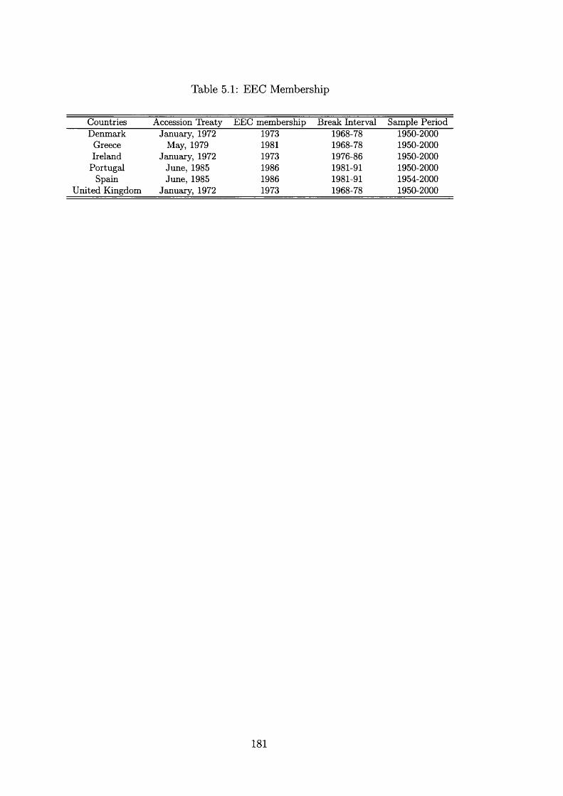
Table 5.1: EEC Membership
Countries Accession Treaty EEC membership Break Interval Sample PeriodDenmark January, 1972 1973 1968-78 1950-2000
Greece May, 1979 1981 1968-78 1950-2000Ireland January, 1972 1973 1976-86 1950-2000
Portugal June, 1985 1986 1981-91 1950-2000Spain June, 1985 1986 1981-91 1954-2000
United Kingdom January, 1972 1973 1968-78 1950-2000
181

Table 5.2: Change in the Intercept in the Series of Overall Openness
Country Z&A test^ T b SupFt k DUtDenmark {t — stat)
-3.582 1972 2.352 3 1.118
Greece {t — stat)
-5.227** 1975 2.046 1 2.309
Ireland {t — stat)
-4.083 1972 6.374 1 9.194
Portugal {t — stat)
-4.289 1984 5.493 5 -6.478
Spain {t — stat)
-2.541 1987 1.940 2 1.254
United Kingdom {t — stat)
-4.893** 1972 16.205*** 1 4.630
Note: Overall Openness is defined as the ratio of total imports and exports to GDP. The ***, **, and * indicate significance levels at the 1, 5, or 10 percent respectively, t-statistics are reported in parenthesis. Tb, k, and SupFt refer to the year of the break, the degree of autocorrelation, and the Wald statistics for the sequential structural break test (Vogelsang, 1997). DUt is the variable related to the break in the intercept, defined as DUt = 1 if t > Tb, 0 otherwise. ^Zivot and Andrews (1992) statistic for the unit root test versus the alternative hypothesis that the series is stationary with a structural break.
Table 5.3: Change in the Intercept in the Series of EEC Openness
Country Z&A te st^ T b SupFt k DUtDenmark {t — stat)
-3.237 1972 6.156 5 1.699
Greece {t — stat)
-4.580* 1979 7.335* 1 2.392
Ireland {t — stat)
-3.273 1972 19.728* 3 11.204
Portugal{t — stat)
-4.932** 1990 15.522*** 7 -5.921
Spain {t — stat)
-4.935** 1986 8.841* 8 1.784
United Kingdom {t - stat)
-4.712* 1972 10.899** 6 2.881
Note: EEC Openness is defined as the ratio of imports and exports to the twelve countries that were members of the EEC by 1986. The ***, **, and * indicate significance levels at the 1, 5, or 10 percent respectively, t-statistics are reported in parenthesis. T b , k, and SupFt refer to the year of the break, the degree of autocorrelation, and the Wald statistics for the sequential structural break test (Vogelsang, 1997). DUt is the variable related to the break in the intercept, defined as DUt = 1 if t > Tb, 0 otherwise. ^Zivot and Andrews (1992) statistic for the unit root test versus the alternative hypothesis that the series is stationary with a structural break.
182

Table 5.4: Change in the Intercept in the Series of GDP (log)
Country Z&A test^ T b SupFt k DUtDenmark -2.192 1976 3.218 4 -0.026
Greece -3.143 1975 3.609 3 0.070(1.9001)
Ireland -4.825** 1967 8.621* 2 0.069
Portugal -4.025 1986 23.893*** 4 -0.127
Spain -2.854 1987 5.250 3 -0.045
United Kingdom -4.768* 1969 13.348*** 7 0.056
Note: The ***, **, and * indicate significance levels at the 1, 5, or 10 percent respectively, t-statistics are reported in parenthesis. Tb, /c, and SupFi refer to the year of the break, the degree of autocorrelation, and the Wald statistics for the sequential structural break test (Vogelsang, 1997). DUt is the variable related to the break in the intercept, defined as DUt = 1 if t > Tg, 0 otherwise. ^Zivot and Andrews (1992) statistic for the unit root test versus the alternative hypothesis that the series is stationary with a structural break.
Table 5.5: Change in the Intercept in the Series of Per-Capita GDP (log)
Country Z&A test^ T b SupFt k DUtDenmark -2.274 1976 3.021 4 -0.025
Greece -3.393 1975 3.362 3. 0.067
Ireland -4.540 1967 9.811 2. 0.070
Portugal -4.738* 1986 18.011** 4 -0.125
Spain -1.792 1987 5.135 3 -0.044
United Kingdom -3.654 1969 13.144 7 0.057
Note: The ***, **, and * indicate significance levels at the 1, 5, or 10 percent respectively, t-statistics are reported in parenthesis. T b , k, and SupFt refer to the year of the break, the degree of autocorrelation, and the Wald statistics for the sequential structural break test (Vogelsang, 1997). DUt is the variable related to the break in the intercept, defined as DUt = 1 if t > T b , 0 otherwise. ^Zivot and Andrews (1992) statisticfor the unit root test versus the alternative hypothesis that the series is stationary with a structural break.
183

Table 5.6: Change in the Intercept in the Series of GDP Growth Rates
Country Z&A test^ Tb SupFt k DUtDenmark -5.649*** 1976 6.649 3 -1.912
Greece -5.571*** 1985 0.536 3 -1.481
Ireland -6.229*** 1967 4.619 1 3.524
Portugal -4.835** 1986 9.873** 3 -5.173
Spain -4.794* 1983. 9.889** 8 -4.466
United Kingdom -4.755* 1975 2.740 6 -1.614(-1.6553)
Note: The ***, **, and * indicate significance levels at the 1, 5, or 10 percent respectively, t-statistics are reported in parenthesis. Tb, k, and SupFt refer to the year of the break, the degree of autocorrelation, and the Wald statistics for the sequential structural break test (Vogelsang, 1997). DUt is the variable related to the break in the intercept, defined as DUt = 1 if t > Tb, 0 otherwise. ^Zivot and Andrews (1992) statistic for the unit root test versus the alternative hypothesis that the series is stationary with a structural break.
Table 5.7: Change in the Intercept in the Series of Relative GDP
Country Z&A test^ Tb SupFt k DUtDenmark -5.372*** 1974 3.347 1 0.026
Greece -5.586*** 1985 2.851 2 -0.041(-1.6880)
Ireland -1.515 1976 11.576** 7 0.1060
Portugal -6.281*** 1987 10.176** 2 -0.151(-3.1899)
Spain -10.627*** 1991 5.986 7 -0.104
United Kingdom -4.314 1967 3.386 2 0.048(1.8401)
Notes: The ***, **, and * indicate significance levels at the 1, 5, or 10 percent respectively, t-statistics are reported in parenthesis. Tb, k, and SupFt refer to the year of the break, the degree of autocorrelation, and the Wald statistics for the sequential structural break test (Vogelsang, 1997). DUt is the variable related to the break in the intercept, defined as DUt = 1 if > Tb, 0 otherwise. ^Zivot and Andrews (1992) statistic for the unit root test versus the alternative hypothesis that the series is stationary with a structural break.
184
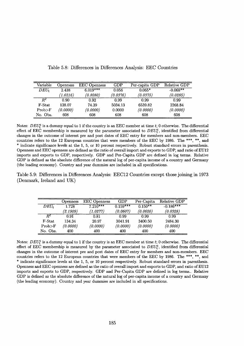
Table 5.8: Differences in Differences Analysis: EEC Countries
Variable Openness EEC Openness GDP Per-capita GDP Relative GDPDEUt 2.438 6.019*** 0.056 0.065* -0.068**
0.90 0.92 0.99 0.99 0.99F-Stat 138.07 74.39 5034.13 6539.82 2268.84
Prob>F (0.0000) (0.0000) 0.0000 (0.0000) (0.0000)No. Obs. 608 608 608 608 608
Notes: DEU^ is a dummy equal to 1 if the country is an EEC member at time t; 0 otherwise. The differential effect of EEC membership is measured by the parameter associated to DEU^, identified from differential changes in the outcome of interest pre and post dates of EEC entry for members and non-members. EEC countries refers to the 12 European countries that were members of the EEC by 1986. The ***, **, and * indicate significance levels at the 1, 5, or 10 percent respectively. Robust standard errors in parenthesis. Openness and EEC openness are defined as the ratio of overall import and exports to GDP, and ratio of EU12 imports and exports to GDP, respectively. GDP and Per-Capita GDP are defined in log terms. Relative GDP is defined as the absolute difference of the natural log of per-capita income of a country and Germany (the leading economy). Country and year dummies are included in all specifications.
Table 5.9: Differences in Differences Analysis: EEC12 Countries except those joining in 1973 (Denmark, Ireland and UK)
Openness EEC Openness GDP Per-Capita Relative GDPDEUt 1.728
(2.1909)7.210*** 0.159***
fO. 0(^07)0.150**fo.ogjgo;
-0.186***
0.91 0.81 0.99 0.99 0.99F-Stat 134.34 20.97 3041.91 3400.50 2484.30
Prob>F (0.0000) (0.0000) (0.0000) (0.0000) (0.0000)No. Obs. 400 400 400 400 400
Notes: DEU^ is a dummy equal to 1 if the country is an EEC member at time t\ 0 otherwise. The differential effect of EEC membership is measured by the parameter associated to DEU^, identified from differential changes in the outcome of interest pre and post dates of EEC entry for members and non-members. EEC countries refers to the 12 European countries that were members of the EEC by 1986. The ***, **, and * indicate significance levels at the 1, 5, or 10 percent respectively. Robust standard errors in parenthesis. Openness and EEC openness are defined as the ratio of overall import and exports to GDP, and ratio of EU12 imports and exports to GDP, respectively. GDP and Per-Capita GDP are defined in log terms.. Relative GDP is defined as the absolute difference of the natural log of per-capita income of a country and Germany (the leading economy). Country and year dummies are included in all specifications.
185
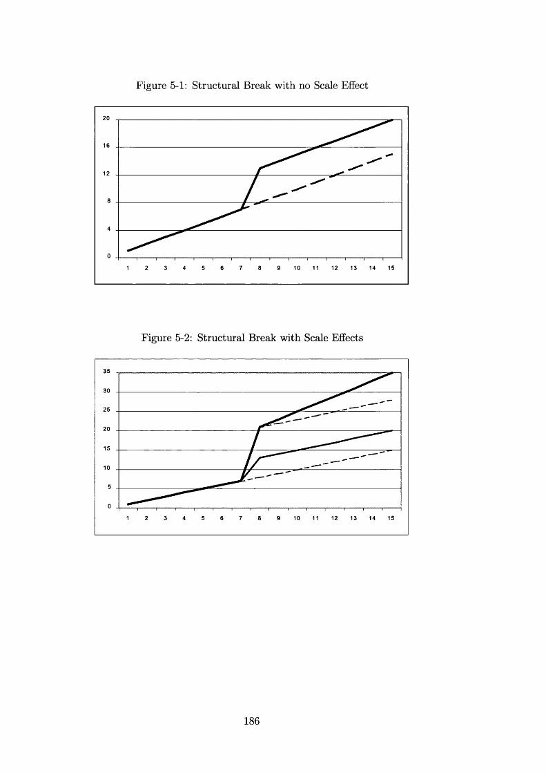
Figure 5-1: Structural Break with no Scale Effect
20
14
Figure 5-2: Structural Break with Scale Effects
35
30
25
20
186

Chapter 6
Conclusions
The primary motivation of this thesis is to understand the economic effects of European integration,
with respect to both the pattern of industrial specialisation in European regions, and openness and
income.
The descriptive analysis in the second chapter provides a panoramic view of patterns of spe
cialisation at the country and regional levels. The chapter contributes to the existing literature in
the following ways. First, it combines country and regional-level data to provide a detailed analysis
of the evolution of patterns of specialisation in European countries. Second, in contrast to the
majority of the existing literature, it uses a theory-consistent measure derived directly from the
neoclassical trade theory as the basis of the analysis. Third, the dynamics of the entire distribution
of the pattern of specialisation is estimated using a statistical model of distribution dynamics.
The analysis suggests, first, that regional GDP shares vary markedly. Variation is higher
across regions than across countries, indicating that regions are more specialised than countries.
Second, there is evidence of some variation across regions, but no evidence of major changes in
the industrial structure of countries and regions over the sample period. Pairwise correlations
indicate that, in general, country’s patterns of specialisation are becoming more dissimilar over
time, with substantial heterogeneity in the degree of similarity in specialisation at the regional level.
Analysing specialisation relative to Europe, countries and regions show increasing specialisation in
manufacturing industries, although specialisation patterns progress at a slow pace.
An accounting decomposition indicates that changes in specialisation at the country level are
mainly due to changes in specialisation at the regional level. There is no evidence of significant
between-region changes, and the relative importance of regions seems to remain fairly constant
over the sample period. The results show that within-region changes in specialisation are more
important in accounting for changes in specialisation at the country level than changes in the
187

shares of regions in a country’s overall economic activity. Regions are changing their pattern of
specialisation more than countries, as the within-region change is typically higher in value than
the total change. Changes in regional shares of GDP do play a small role in explaining changes in
specialisation at the country level for the disaggregated manufacturing industries.
Finally, there is no evidence of an increase in the overall degree of specialisation over time, but
of significant mobility. The analysis of the distribution dynamics indicate certain polarisation of
the distribution of GDP shares towards the bottom two quintiles for most of the countries and
regions under analysis. We find evidence of substantial mobility in patterns of specialisation at the
country and regional levels. Mobility suggests significant changes in the patterns of specialisation.
In general, regions display higher mobility in their patterns of specialisation, although differences
can be found, depending on the regions and countries considered. Also, there is evidence of higher
mobility in the middle quintiles and higher persistence in the extreme quintiles of the distribution
at the regional level. Comparing the initial and the ergodic distribution, there is a general pattern
of polarisation toward the three lowest quintiles of the distribution at the country and regional
levels. Additionally, we find evidence of within-country differences in the evolution of the patterns of
specialisation. Out of 45 of the regions, 31 follow a dynamic process that is statistically significantly
different from the one at the country level.
Chapters 3 and 4 analyse the determinants of specialisation. Chapter 3 considers solely the role
of factor endowments in explaining the patterns of specialisation at the regional level in Europe.
Our main empirical findings are as follows. First, the HO model provides an incomplete explanation
of patterns of production across European regions and is rejected against more general neoclassical
alternatives. Second, although the HO model is rejected, factor endowments remain statistically
significant and quantitatively important in explaining production structure within different neoclas
sical alternatives. Individual factor endowments are highly statistically significant and including
information on factor endowments reduces the model’s within-sample average absolute prediction
error by a factor of around three in Manufacturing.
Third, the pattern of estimated coefficients on factor endowments across industries is generally
consistent with economic priors regarding factor intensity. For example, physical capital endow
ments are positively correlated with the share of Manufacturing in GDP and negatively correlated
with the shares of Agriculture and Services. Higher numbers of medium education individuals
relative to low education individuals are associated with a lower share of Agriculture in GDP and
a higher share of Manufacturing. Higher numbers of high education individuals relative to medium
education individuals are associated with a lower share of Manufacturing in GDP and a higher
share of Services.
188
Fourth, factor endowments are more successful in explaining patterns of production at the
aggregate level in Agriculture, Manufacturing and Services (where we have three industries and
either three or five factor endowments) than in disaggregated manufacturing industries (where we
have 11 industries and either three or five factor endowments). Within-sample average absolute
prediction errors are typically far larger in the disaggregated manufacturing industries, and this
is exactly as theory would predict. In the HO model with identical prices and technology and
with no joint production, patterns of production are only determinate if there are at least as many
factors of production as goods. Therefore, production indeterminacy provides one explanation
for larger average absolute prediction errors in disaggregated manufacturing industries. Another
explanation, again consistent with the theory, could be that regional price and technology differences
not controlled for in the right-hand side variables are particularly large in individual manufacturing
industries. Also, economic geography considerations are not controlled for in the analysis.
Finally, we find no evidence that the process of increasing economic integration in Europe has
weakened the relationship between patterns of production and factor endowments across regions
within countries. Examining within-sample prediction errors for this specification reveals no sys
tematic trend over time for either the three aggregate industries or the 11 disaggregated industries
within manufacturing.
As factor endowments alone were not very successful in explaining patterns of specialisation
for the disaggregated manufacturing industries. Chapter 4 incorporates economic geography into
the analysis of the determinants of specialisation in the manufacturing sector across European re
gions. The empirical findings yield the following conclusions. First, both factor endowments and
economic geography are statistically significant in explaining specialisation patterns in manufac
turing industries in European regions. Parameter estimates are relatively constant across different
specifications that take into account different sources of unobserved heterogeneity. Second, the
estimation results are in line with economic priors. Other things being equal, regions with high
education endowments would be more specialised in skill-intensive industries. Among the economic
geography variables, the interaction of access to suppliers and intermediate intensity is statistically
significant in explaining specialisation at the one percent level. Regions with good access to inter
mediate goods attract industries that are more intensive in intermediate goods. Cost linkages are
more important than demand linkages. Third, our model performs well in explaining patterns of
specialisation across European regions. The model’s average prediction error across all disaggre
gated manufacturing industries, regions, and time is 13 percent, and ranges from 8 percent to 20
percent in individual manufacturing industries. Average prediction errors compare positively with
those reported in Chapter 3, where the average prediction error for the same eight manufacturing
189

industries was 58 percent from 1985-95. Furthermore, when using the estimated coefficients to
evaluate predicted shares of GDP excluding information on factor endowments, economic geogra
phy, and industry characteristics; the average prediction error in manufacturing industries rises to
120 percent. Finally, prediction errors remain stable over time, not only within countries, but also
across industries in our sample.
Having found that economic integration has not changed the relationship between patterns of
specialisation and its determinants over time. Chapter 5 uses a more macroeconomic approach to
analyse the effects of EEC membership. The analysis is divided in two sections. First, we investigate
permanent effects of EEC membership. A sequential structural break analysis indicates that EEC
membership improves openness within the EEC permanently. As there is no evidence of permanent
effects on overall openness, it appears that EEC membership has a smaller effect on trade flows, and
these effects could be obscured by changes in other variables, which is consistent with some trade
diversion. There is some evidence of permanent effects on income, with three out of six countries
showing a significant permanent change in the series of CDP in line with openness. Permanent
changes in openness are, however, not reflected in permanent changes in income growth. This could
be the result of other elements affecting income in the opposite direction from openness, e.g., if weak
productivity growth were the case at the time of the break. Three of the countries analysed joined
the EEC at the time of the first oil crisis, which severely affected Western Europe in the first half of
the 1970s. The empirical evidence supports the existence of level effects on income, but not of scale
effects on income growth nor of effects on income convergence as a result of economic integration.
While informative, a problem with the tests for structural breaks with univariate time-series is
that there may be other time-series shocks which affect countries at the same time as their entry
into the EEC. To help address this concern, we use EEC membership as an experiment to shed
further light on its effect on openness, income, and income convergence in Europe by considering a
differences in differences specification which controls for common time series shocks affecting both
EEC members and non-members. Therefore, in the second section, we explore the differential effects
of EEC membership with a difference-in-difference analysis. In contrast with the structural break
analysis, the differences in differences analysis is controlling for common time-series shocks affecting
members and non-members. When differencing out the common time-series effects and focusing
on the differential effects of EEC membership across countries relative to non-members, openness
among the EEC countries improved significantly as a result of new countries entering the EEC, in
line with the results from the structural breaks. We also find level effects on income as a result
of countries joining the EEC. CDP and per-capita CDP improve significantly as countries joined
the EEC. Finally, results also support the idea that joining the EEC improves the convergence
190

process. The coefficient estimate associated to relative income reports the expected (negative) sign
indicating a decrease in income dispersion relative to Germany, the leading economy, and it is
statistically significant.
On the whole, we believe that this thesis makes a contribution to our understanding of the
determinants of specialisation patterns at the regional level in Europe, as well as of the impact of
economic integration on openness, income, and income growth. It also offers some ideas for future
research.
191
ReferencesAghion, P and Howitt, P (1992) “Fundamental Stocks of Knowledge and Productivity Growth” Journal of Political Economy^ 98.
Alcala, F and Ciccone, A (2001) “Trade and Productivity”, CEPR Discussion Paper, no. 3095. London, Centre for Economic Policy Research, London.
Amiti, M (1998) “New Trade Theories and Industrial Location in the EU: A Survey of Evidence”, Oxford Review of Economic Policy, 14(2), 45-53.
Amiti, M (1999) “Specialisation Patterns in Europe”, Weltwirtschaftliches Archiv, 135(4), 573-93.
Anderson, T and Goodman, L (1957) “Statistical Inference About Markov Chains”, Annuals of Mathematical Statistics, 28, 89-110.
Baldwin, R (1994) Towards an Integrated Europe, Centre for Economic Policy Research, London.
Banerjee, A, Lumsdaine, R and Stock, J (1992) “Recursive and Sequential Tests of the Unit Root and Trend Break Hypothesis: Theory and International Evidence” Journal of Business and Economic Statistics, 10.
Barro, R and Sala-i-Martin, X (1995) Economic Growth, McGraw-Hill.
Ben-David, D (1993) “Equalising Exchange: Trade Liberalisation and Income Convergence” Quarterly Journal of Economics, 108, 653-79.
Ben-David, D and Papell, D (1995) “The Great Wars, The Great Crash, and The Unit Root Hypothesis: Some New Evidence about an Old Stylised Fact”, Journal of Monetary Economics, 36 (3), 453-75.
Ben-David, D (1996) “Trade and Convergence among Countries” Journal of International Economics, 40, 279-98.
Ben-David, D and Papell, D (1997) “International Trade and Structural Change” Journal of International Economics, 43, 513-23.
Ben-David, D and Papell, D (1998) “Slowdowns and Meltdowns: Post-war Growth Evidence from 74 Countries” Review of Economics and Statistics, 80, 561-71.
Ben-David, D, Lumsdaine,R and Papell, D (2003) “Unit Roots, Postwar Slowdowns and Long-Run Growth: Evidence from Two Structural Breaks”, Empirical Economics, 303-319.
Bernard, A and Jones, C (1996a) “Productivity across Industries and Countries: Time Series Theory and Evidence” Review of Economics and Statistics, 78(1), 135-46.
Bernard, A and Jones, C (1996b) ‘Comparing Apples to Oranges: Productivity Convergence and Measurement across Industries and Countries’, American Economic Review, December, 1216-38.
Bernstein, J and Weinstein, D (2002) ‘Do Endowments Determine the Location of Production? Evidence from National and International Data’, Journal of International Economics, 56(1), 55-76.
Bowen, H, Leamer, E, and Sveikauskas, L (1987) “Multicountry, Multifactor Tests of the Factor Abundance Theory”, American Economic Review, 77, 791-809.
192
Brülhart, M and Torstesson, J (1996) “Regional Integration, Scale Economies and Industry Location in the European Union”, CEPR Discussion Paper, no. 1435. Centre for Economic Policy Research, London.
Brülhart, M (1998) “Trading Places: Industrial Specialisation in the European Union”, Journal of Common Market Studies, 36(3), 319-44.
Brülhart, M (2001) “Evolving Geographical Specialisation of European Manufacturing Industries”, Weltwirtschaftliches Archiv, 137(2), 215-43.
Brunner, A (2003) “ The Long-Run Effects of Trade on Income and Income Growth” IMF Working Paper no. 37. International Monetary Fund, Washington DC.
Cameron, G and Muellbauer, J (1998) “The Housing Market and Regional Commuting and Migration Costs”, Scottish Journal of Political Economy, 45(4), 420-46.
Cameron, G, Proudman, J and Redding, S (1998) “Productivity Convergence and International Openness” in Openness and Growth, Chapter 6, Bank of England.
Cameron, G, Proudman, J and Redding, S (2003) “Technological Convergence, R&D, Trade and Productivity Growth”, European Economic Review, forthcoming.
Campbell, J and Perron, P “Pitfalls and Opportunities: What Macroeconomists Should Know About Unit Roots”, NBER Macroeconomics Annual, 6 (1991), National Bureau of Economic Research, Cambridge.
Crafts, N and Toniolo, G (1996) Economic Growth in Europe since 1945, Cambridge University Press.
Ciccone, A and Hall, R (1996) “Productivity and the Density of Economic Activity”, American Economic Review, 86(1), 54-70.
Coe, D and Helpman, E (1995) “International R&D Spillovers”, European Economic Review, 39(5), 859-87.
Combes, P and Overman, H (2003) “The Spatial Distribution of Economic Activities in the EU”, CEPR Discussion Paper, no. 3999. Centre for Economic Policy Research, London. Paper prepared for the Handbook of Urban and Regional Economics, Volume 4 edited by J. Vernon Henderson and Jacques Thisse.
Davis, D and Reeve, T (1997) “Human Capital, Unemployment, and Relative Wages in a Global Economy”, NBER Working Paper, no. 6133. National Bureau of Economic Research, Cambridge.
Davis, D, Weinstein, D, Bradford, S, and Shimpo, K (1997) “Using International and Japanese Regional Data to Determine When the Factor Abundance Theory of Trade Works”, American Economic Review, 87(3), 421-46.
Davis, D and Weinstein, D (1996) “Does Economic Geography Matter for International Specialization?” , NBER Working Paper, no. 5706. National Bureau of Economic Research, Cambridge.
Davis, D and Weinstein, D (1999) “Economic Geography and Regional Production Structure: An Empirical Investigation”, European Economic Review, 43, 379-407.
Davis, D and Weinstein, D (2001) “An Account of Global Factor Trade”, American Economic
193
Review, 91(5), 1423-53.
Davis, D and Weinstein, D (2003) “Market Access, Economic Geography, and Comparative Advantage: An Empirical Assessment”, Journal of International Economics, 59(1), 1-23.
Deardoff, A (1974) “Factor Proportions and Comparative Advantage in the Long-Run: Comment”, Journal of Political Economy, 82(4), 829-33.
Devereux, M, Griffith, R, and Simpson, H (1999) “The Geographic Distribution of Productive Activity in the UK”, Institute for Fiscal Studies Working Papers no. 26.
Dixit, A and Norman, V (1980) The Theory of International Trade, Cambridge University Press, Cambridge.
Dollar, D (1992) “ Outward-Oriented Developing Economies Really Do Crow More Rapidly: Evidence from 95 LDCs, 1976-1985”, Economic Development and Cultural Change, 523-44.
Duranton, C and Overman, H (2002) “Testing for Localization Using Micro-Geographic Data”, CEPR Discussion Paper no. 3379. Centre for Economic Policy Research, London.
Eaton, J (1987) “A Dynamic Specific-Factor Model of International Trade”, Review of Economic Studies, 325-38.
Edwards, S (1998) “Openness, Productivity and Growth: What Do We Really Know?”, Economic Journal, 108.
Edwards, S (1992) “Trade Orientation, Distortions and Growth in Developing Countries”, Journal of Development Economics, 39.
Ethier, W (1984) ‘Higher Dimensional Issues in Trade Theory’, Chapter 3 in (eds) Jones, R and Kenen, P, Handbook of International Economics, I, 131-84.
Ellison, C, and Claeser, E (1997) “Geographic Concentration in US Manufacturing Industries: A Dartboard Approach”, Journal of Political Economy, 105(5), 889-927.
Ellison, C, and Claeser, E (1999) “The Geographic Concentration of Industry: Does Natural Advantage Explain Agglomeration?”, American Economic Review, 89(2), Papers and Proceedings, 311-16.
Feenstra, R, Markusen, J, and Rose, A (2001) “Using the Gravity Model to Differentiate Among Alternative Theories of Trade”, Canadian Journal of Economics, 34(2), 430-47.
Findlay, R (1970) “Factor Proportions and Comparative Advantage in the Long Run”, Journal of Political Economy, 78(1), 27-34.
Forlisd, R, Haaland, J, and Midelfart-Knarvik, K (2002) “A U-Shaped Europe? A Simulation Study of Industrial Location”, Journal of International Economics, 57, 273-97.
Frankel, J and Romer, D (1999) “ Does Trade Cause Growth?”, American Economic Review, 89(3), 379-399.
Fujita, M, Krugman, P, and Venables, A (1999) The Spatial Economy: Cities, Regions, and International Trade, MIT Press.
Cabaix, X (1997) “The Factor Content of Trade: A Rejection of the Heckscher-Ohlin-Leontief
194

Hypothesis”, mimeograph, Harvard University.
Gandal, N, Hanson, G, and Slaughter, M (2002) “Technology, Trade, and Adjustment to Immigration in Israel”, European Economic Review forthcoming.
Geweke, J, Marshall, R, and Zarkin, G (1986) “Mobility Indices in Continuous Time Markov Chains”, Econometrica, 54, 1407-23.
Giannetti, M “The Effects of Integration on Regional Disparities: Convergence, Divergence, or Both?”, mimeograph, Stockholm School of Economics.
Griffith, R, Redding, S, and Van Reenen, J (2000) ‘Mapping the Two Faces of R&D: Productivity Growth in a Panel of OECD Manufacturing Industries’, CEPR Discussion Paper no. 2457, Centre for Economic Policy and Research, London.
Griliches, Z and Hausman, J (1986) “Errors in Variables in Panel Data”, Journal of Econometrics, 31, 93-118.
Grossman, G and Helpman, E (1991a) Innovation and Growth in the Global Economy, MIT Press, Cambridge MA.
Grossman, G and Helpman, E (1991b) “Quality Ladders and Product Cycles” Quarterly Journal of Economics, 106.
Haaland, J, Kind, H, Midelfart-Knarvik, K, and Torstensson, J (1999) “What Determines the Economic Geography of Europe?”, CEPR Discussion Paper, no. 2072. Centre for Economic Policy Research, London.
Hallet, M (2000), “Regional Specialisation and Concentration in the EU”, Economic Papers no. 141. Directorate-General for Economic and Financial Affairs of the European Commission.
Hanson, G (1998) “North American Economic Integration and Industry Location”, Oxford Review of Economic Policy, 14(2), 30-44.
Hanson, H and Slaughter, M (2002) “Labor Market Adjustment in Open Economies: Evidence from US States”, Journal of International Economics, forthcoming.
Harrigan, J (1995) “Factor Endowments and the International Location of Production: Econometric Evidence for the OECD, 1970-85”, Journal of International Economics, 39, 123-41.
Harrigan, J (1997) “Technology, Factor Supplies, and International Specialisation: Estimating the Neoclassical Model”, American Economic Review, 87(4), 475-94.
Harrigan, J and Zakrajsek, E (2000) “Factor Supplies and Specialisation in the World Economy”, NBER Working Paper no. 7848. National Bureau of Economic Research, Cambridge.
Harrison, A (1996) “Openness and Growth: a Time-Series, Cross-Country Analysis for Developing Countries”, Journal of Development Economics, 48, 419-447.
Harrison, A and Hanson, G (1999) “Who Gains from Trade Reform? Some Remaining Puzzles?” Journal of Development Economics, 59, 125-154.
Head, K and Ries, J (2001) “Increasing Returns versus National Product Differentiation as an Explanation for the Pattern of US-Canada trade”, American Economic Review, 91(4), 858-76.
195

Helpman, E (1981) “International Trade in the Presence of Product Differentiation, Economies of Scale, and Monopolistic Competition: A Chamberlin-Heckscher-Ohlin Approach”, Journal of International Economics, 11(3), 305-40.
Helpman, E (1984) “Increasing Returns, Imperfect Markets, and Trade Theory”, Chapter 7 in (eds) Jones, R and Kenen, P, Handbook of International Economics, I, 325-65.
Helpman, E and Krugman, P (1985) Market Structure and Foreign Trade, MIT Press.
Henderson, J (1999) “Marshall’s Scale Economies” NBER Working Paper no. 7345. National Bureau of Economic Research, Cambridge.
Hendry, D and Mizon, G (1998) “Exogeneity, Causality, and Co-Breaking in Economic POlicy Analysis of a Samll Econometric Model of Money in the UK”, Empirical Economics, 23, 267-95.
Hendry, D (1999) “A Theory of Co-breaking”, in Forecasting Non-stationary Economic Times Series, MIT Press, with M.P. Clements.
Im, K, Pesaran, M, and Shin, Y (2003) “Testing for Unit Roots in Heterogeneous Panels”, Journal of Econometrics, 115, 53-74.
Irwin, D and Tervio, M (2000) “Does Trade Raise Income? Evidence from the Twentieth Century”, NBER Working Paper no. 7745. National Bureau of Economic Research, Cambridge.
Jones, C (1995) “Time Series Test of Endogenous Growth Models” Quarterly Journal of Economics, 110, 495-525.
Jones, C (1999) “Growth: With or Without Scale Effects?” American Economy Review Papers and Proceedings, 89, 134-144.
Keller, W (1997) “Are International R&D Spillovers Trade-related? Analyzing Spillovers among Randomly Matched Trade Partners”, European Economic Review, 42, 1469-81.
Kremer, M, Onatski, A, and Stock, J (2001) “Searching for Prosperity”, National Bureau of Economic Research Working Paper no. 8250.
Kim, S (1995) “Expansion of Markets and the Geographic Distribution of Economic Activities: The Trends in U.S. Regional Manufacturing Structure, 1860-1987”, Quarterly Journal of Economics, 110(4), 881-908.
Kohli, U (1991) Technology, Duality and Foreign Trade, Ann Arbor: University of Michigan Press.
Krugman, P (1981) “Intra-industry Specialization and the Gains from Trade”, Journal of Political Economy, 89(5), 959-74.
Krugman, P (1987) “The Narrow Moving Band, the Dutch Disease and the Competitive Consequences of Mrs. Thatcher: Notes on trade in the Presence of Scale Economies”, Journal of Development Economics, 27, 41-55.
Krugman, P (1991a) “Increasing Returns and Economic Geography”, Journal of Political Economy, 99(3), 483-99.
Krugman, P (1991b) Geography and Trade, MIT Press, Gambridge.
Krugman, P, and Venables, A (1990) “Integration and the Competitiveness of the Peripheral In-
196
dustry”, in C. Bliss and J. Braga de Macedo,(eds), Unity with Diversity in the European Economy: The Community’s Southern Frontier, Cambridge University Press, Cambridge.
Krugman, P, and Venables, A (1995) “Globalization and the Inequality of Nations”, Quarterly Journal of Economics, 857-80.
Leamer, E (1980) “The Leontief Paradox Reconsidered”, Journal of Political Economy, 88(3), 495- 503.
Leamer, E (1984) Sources of Comparative Advantage: Theories and Evidence, MIT Press.
Leontief, W (1953) “Domestic Production and Foreign Trade: The American Capital Position Re-examined”, Proceedings of the American Philosophical Society, 97, 332-49.
Levin, A and Lin, C (1992) “Unit Root Tests in Panel Data: Asymptotic and Finite-sample Properties” , University of California, San Diego, Discussion Paper no. 23.
Lichtenberg, F and van Pottelsberghe de la Potterie, B (2001) “Does Foreign Direct Investment Transfer Technology across Borders”, Review of Economics and Statistics, 83(3), 490-7.
Machin, S and Van Reenen, J (1998) “Technology and Changes in Skill Structure: Evidence from Seven OECD Countries”, Quarterly Journal of Economics, November, 1215-44.
Maddala, G and Wu, S (1999) “A Comparative Study of Unit Root Tests with Panel Data and a New Simple Test”, Oxford Bulletin of Economics and Statistics, Special Issue, 631-52.
Magrini, S (1999) “ The Evolution of Income Disparities among the Regions in the European Union”, Regional Science and Urban Economics, 29, 257-81.
Maurel, F and Sedillot, B (1999) “ A Measure of the Geographic Goncentration in French Manufacturing Industries”, Regional Science and Urban Economies, 29(5), 575-604.
McCormick, B (1997) “Regional Unemployment and Labour Mobility in the United Kingdom”, European Economic Review, 41(3-5), 581-89.
Midelfart-Knarvik, K, Overman, H, Redding, S, and Venables, A (2000a) “The Location of European Industry”, report prepared for the Directorate General for Economic and Financial Affairs, European Commission, Economic Papers no. 142, April 2000. European Commission, Brussels.
Midelfart-Knarvik, K, Overman, H and Venables, A (2000b) “Comparative Advantage and Economic Geography: Estimating the Location of Production in the EU”, CEPR Discussion Paper, no. 2618. Centre for Economic Policy Research, London.
Midelfart-Knarvik, K, and Overman, H (2002) “Delocation and European Integration: Is Structural Spending Justified?”, Economic Policy 35, 323-59.
Midelfart-Knarvik, K, Overman, H, and Venables, A (2003) “Monetary Union and the Economic Geography of Europe”, mimeograph, London School of Economics.
Molle, K (1997) “The Regional Economic Structure of the European Union: An Analysis of the Long-Term Developments”, in K. Peschel, ed.. Regional Growth and Regional Policy Within the Framework of European Integration (Physica-Verlag, Heidelberg), 66-86.
Moulton, B (1986) “Random Group Effects and the Precision of Regression Estimates”, Journal of
197
Econometrics, 32, 385-97.
Ng, S and Perron, P (1995) “Unit Root Test in ARMA Models with Data Dependent Methods for the Selection of the Truncation Lag”, Journal of the American Statistical Association, 90.
Nickell, S and Bell, B (1996) “Changes in the Distribution of Wages and Unemployment in OECD Countries”, American Economic Review, 86(2), 302-8.
Nickell, S, Redding, S, and Swaffield, J (2001) “Labour Market Institutions and the Structure of Production”, CEPR Discussion Paper no. 3068. Centre for Economic Policy Research, London.
Norman, V (2000) Unpublished Notes on Trade and Location, Nowergian School of Economic and Business Administration.
Norman, V and Venables, A (1995) “International Trade, Factor Mobility, and Trade Costs”, Economic Journal, 105.
Overman, H, Redding, S, and Venables, A (2001) “The Economic Geography of Trade, Production, and Income; A Survey of Empirics”, forthcoming in Harrigan, J. (Ed.), Handbook of International Trade, Basil Blackwell, Oxford. Also CEPR Discussion Paper no. 2978. Centre for Economic Policy Research, London.
Pedroni, P (1999) “Critical Values for Cointegration Tests in Heterogeneous Panels with Multiple Regressors”, Oxford Bulletin of Economics and Statistics, Special Issue, 653-70.
Pesaran, M, Shin, Y, and Smith, R (1999) “Pooled Mean Group Estimation of Dynamic Heterogeneous Panels”, Journal of the American Statistical Association, 94, 621-34.
Perron, P (1997) “Further Evidence on Breaking Trend Functions in Macroeconomic Variables”, Journal of Econometrics, 80.
Perron, P (1989) “Testing for a Unit Root in a Time Series with a Changing Mean”, Journal of Business & Economic Statistics, 8(2).
Perron, P (1990) “The Great Crash, the Oil Price Shock and the Unit Root Hypothesis”, Econometrica, 57.
Prichett, L (1996) “Measuring Outward Orientation in LDCs: Can It Be Done?”, Journal of Development Economics, 49(2), 307-35.
Proudman, J and Redding, S (1998) “Persistence and Mobility in International Trade”, Chapter 2 in (eds) Proudman, J and Redding, S, Openness and Growth, Bank of England.
Proudman, J and Redding, S (2000) “Evolving Patterns of International Trade”, Review of International Economics, August, 8(3), pages 373-96.
Puga, D (2001) “ European Regional Policies in light of Recent Location Theories”, CEPR Discussion Paper, no. 2767. Centre for Economic Policy Research, London.
Quah, D (1993) “Empirical Cross-Section Dynamics in Economic Growth”, European Economic Review, 37, 426-34.
Quah, D (1994) “Exploiting Cross-section Variation for Unit Root Inference in Dynamic Data”, Economics Letters, 44, 9-19.
198

Quah, D (1996a) “Twin Peaks: Growth and Convergence in Models of Distribution Dynamics”, Economic Journal, 106, 1045-55.
Quah, D (1996b) “Convergence Empirics Across Economies with (some) Capital Mobility”, Journal of Economic Growth, 1, 95-124.
Quah, D (1996c) “Aggregate and Regional Disaggregate Fluctuations”, Empirical Economics, 21, 137-59.
Redding, S (2002) “Specialisation Dynamics”, Journal of International Economics, 58(2), 299-334.
Redding, S and Vera-Martin, M (2003) “Factor Endowments and Production in European Regions”, CEPR Discussion Paper, no. 3755. Centre for Economic Policy Research, London.
Renelt, D and Ross, L (1992) “A Sensitivity Analysis of Cross-Country Growth Regressions” American Economic Review, 82(4), 942-63.
Rodriguez-Pose, A (1999) “Convergence or Divergence? Types of Regional Responses to Socio- Economic Change in Western Europe?”, Tijdchrift voor Economische en Sociale Geografie, 90-4, 363-378.
Rodriguez, F and Rodrik, D (1999) “Trade Policy and Economic Growth: A Skeptic’s Guide to the Cross-National Evidence”, NBER Working Paper no. 7081. National Bureau of Economic Research, Cambridge.
Romer, P (1990) “Endogenous Technological Change” Journal of Political Economy, 94.
Sachs, J and Warner, A (1995) “ Economic Reform and the Process of Global Integration”, Brookings Papers on Economic Activity, 1995(1), 1-118.
Slaughter, M (1998) “ International Trade and Per-capita Income Convergence: A Difference-in- Differences Analysis”, Journal of International Economics, 55(1), 203-28.
Shorrocks, A (1978) “The Measurement of Mobility”, Econometrica, 46, 1013-24.
Trefler, D (1995) “The Case of the Missing Trade and Other Mysteries”, American Economic Review, 85(5), 1029-46.
Urwin, D (1995) The Community of Europe: A History of European Integration since 1945, Longman Croup UK, 2nd edition.
Venables, A (1996) “Equilibrium Locations of Vertically Linked Industries”, International Economic Review, 37, 341-59.
Vogelsang, T (1997) “Wald-Type Tests for Detecting Breaks in the Trend Function of a Dynamic Time Series” Econometric Theory 13.
Woodland, A (1982) International Trade and Resource Allocation, North Holland: Amsterdam.
Zivot, E and Andrews, W (1992) “Further Evidence on the Great Crash, the Oil-Price Shock, and the Unit-Root Hypothesis” Journal of Business and Economic Statistics, 10(3).
199