MSc Modern Applications of Mathematics

Growth of Value in Social Networks

Author:Ruth Jenkins

Supervisors:Professor Chris Budd

Shail Patel

September 2008

Declaration: I certify that all work contained within this document is myown, unless otherwise referenced.

Ruth Jenkins

Abstract

Metcalfe’s Law states that the value of a communications network grows withthe square of the size of the network. Metcalfe, however, could well havebeen misquoted. The validity, or not, of Metcalfe’s Law is critical in a timewhen companies are valuing themselves, using this rough rule of thumb as ajustification. Does Metcalfe’s Law actually hold for online social networks?

This project seeks to review current social network models and look intomethods of valuing them. We will explain the basis of Metcalfe’s Law, aswell as other theoretical value models and examine empirical data to test thevalidity of both the network models and the value metrics.

Finally we present a dynamic model of an online social network and measureits value growth. In fact, it turns out that Metcalfe is a long way off themark.

Contents

1 Introduction 3

2 Social Network Structure 4

2.1 Observed Characteristics of a Social Network . . . . . . . . . . 5

2.1.1 Definitions . . . . . . . . . . . . . . . . . . . . . . . . . 5

2.1.2 Characteristic Values . . . . . . . . . . . . . . . . . . . 7

2.2 Historical and Current Social Network Models . . . . . . . . . 9

2.2.1 The Erdos and Renyi Random Network . . . . . . . . . 9

2.2.2 The Watts and Strogatz Small World Model . . . . . . 10

2.2.3 The Barabasi-Albert Model of Preferential Attachment 11

2.2.4 The Davidsen Model of Introduction . . . . . . . . . . 13

3 Calculating Value Growth 16

3.1 Theoretical Approaches to Value Growth . . . . . . . . . . . . 16

3.1.1 Linear growth . . . . . . . . . . . . . . . . . . . . . . . 16

3.1.2 Metcalfe’s Law . . . . . . . . . . . . . . . . . . . . . . 17

3.1.3 Reed’s Law . . . . . . . . . . . . . . . . . . . . . . . . 18

3.1.4 Zipf functions and Value as a Harmonic Series . . . . . 18

1

3.2 Empirical Research of Value Growth in a Social Network . . . 20

3.2.1 Dunbar’s Chistmas Card Questionnaire . . . . . . . . . 20

3.2.2 Value Growth of an Online Social Network . . . . . . . 20

3.2.3 Primary Data From ’Facebook’: Investigating Valueper User . . . . . . . . . . . . . . . . . . . . . . . . . . 22

3.3 From Value to the Individual to Value of the Network . . . . . 32

4 Developing A Model 34

4.1 Verifying Existing Results . . . . . . . . . . . . . . . . . . . . 35

4.2 Model Requirements . . . . . . . . . . . . . . . . . . . . . . . 35

4.3 Final Model . . . . . . . . . . . . . . . . . . . . . . . . . . . . 40

5 Conclusions 43

5.1 Results of the Model . . . . . . . . . . . . . . . . . . . . . . . 43

5.2 Review of the Model and Suggestions for Further Work . . . . 46

A Derivation of n ln(n) Value Growth 52

B Finite Sum of the Harmonic Series 53

C Matlab Code 54

2

Chapter 1

Introduction

The dot-com bubble of the late nineteen-nineties was due, in large part,to the market’s belief in Metcalfe’s Law. Metcalfe’s Law states that thevalue of a communications network grows proportionally to the square of itssize. The dot-com entrepreneurs chased market share, not profits, since itwas believed that once the size of the business was big enough Metcalfe’sLaw would kick in and provide profits on a quadratic scale. Unfortunatelyfor these small businesses they had misinterpreted Metcalfe - the bubbleburst. Between March 2002 and October 2002 five trillion dollars in marketvalue was lost from technology companies, triggering a mini recession in theWestern economies.

We are now entering a new era of online provision. The web is moving awayfrom information dissemination and toward networking; with interactionsbetween groups. These social networking applications, for example Facebook,Secondlife, Myspace and Flickr, are currently seeing the same unrealisticallyhigh valuations being placed on them as was placed upon their nineteen-nineties counterparts [19]. What is the relationship between growth andvalue? Does Metcalfe’s Law now apply?

This report aims to investigate various existing models of social networksand explore several value forming processes. This report will then look atempirical data to determine which models best reflect reality. Finally we willdevelop a model of online social network value growth.

3

Chapter 2

Social Network Structure

Mathematicians seriously began to involve themselves in social network anal-ysis about half a century ago. Network analysis had been around as a branchof pure mathematics for some time before this, but Pool and Kochen [31]were the first to apply a mathematical model to the social sciences. Pool andKochen investigated chain lengths connecting people and the probability oftwo people knowing each other. This early work used the random networkas a model. We will see below that a random network models a few, but notmany, of the features of a social network. More accurate and refined modelshave now been produced.

The first question is naturally then, how do we know what an accurate modellooks like? This chapter begins with a section addressing that question. Wewill look at empirical data from real world networks and define measures thatwill be important to retain in the models.

This chapter will then examine several different models and consider theirstrengths and weaknesses as candidates for a social network. The models tobe reviewed are:

• The random network

• The Watts-Strogatz ’small world’ network

• The Barabasi-Albert model of preferential attachment

• The Davidsen model of introduction

4

2.1 Observed Characteristics of a Social Net-

work

Real networks are complicated objects. We need to extract their key fea-tures, whilst retaining a manageable model. We consider the three featuresconsidered most important [26]:

• average path length, how many intermediary acquaintances exist be-tween two randomly chosen people?

• clustering coefficient, how much more likely are you to know someoneif you have a mutual friend?

• degree distribution, are we all equally popular or do some people havemore friends than others?

Some real world analysis [23, 26, 28] informs us that social networks arecharacterised by:

• high clustering, people tend to form friendship groups

• short average path length, the famous, and perhaps surprising fact,realised in Milgram’s ’six degrees of separation’ experiment [23]

• a power law degree distribution, we like to make friends with popularpeople

We will firstly define these measures more precisely and then go on to lookat some actual empirical data.

2.1.1 Definitions

Average Path Length

The path length, l(i, j), is the fewest number of edges between nodes i andj, with the average path length, L, being the average taken over all pairs ofnodes with finite path length.

5

Clustering

Clustering feels intuitively straightforward; groups of friends will form withina larger network. It is however, fairly difficult to measure and has beendefined in different ways by different people. Watts and Strogatz [35] defineit as follows:

If node i has ki neighbours, then the maximum number of connections be-tween these neighbours is 1

2ki(ki − 1). Let Ci denote the fraction of these

connections that actually exist. Then the clustering coefficient across thenetwork is the sum of these, i.e.

C =1

n

n∑i=1

Ci

The problem with this definition is that a person with very few friends isgiven the same weighting as a person with many friends (and hence a fewsmall, tightly knit cliques will outweigh larger, more loosely connected sub-networks). This can be seen to erode the value of C for networks with a largevariance across the degree distribution [28]. Newman et al [27] redefined theclustering coefficient to take account of this. They proposed the following:

Cnew =3× number of triangles

number of connected triples

where a connected triple is node connected to two other nodes, and a triangledemands that these two other nodes are also connected to each other.

The intuition of this definition is similar, what percentage of a person’sfriends are themselves friends? Whilst it is better suited to networks withlarge variance at degree, it is more difficult to calculate. We will use theWatts-Strogatz definition unless otherwise stated as it is the more commonlyunderstood definition in literature [8].

Degree Distribution

Thinking qualitatively about social networks is does not seem reasonable thatall nodes should have equal degree, it is just a fact of life that some peopleare more popular than others. The degree distribution tells us how manynodes have a given degree.

6

Analysis of real networks tells us that popular people haven’t just got a lotof friends, they are also good at making new friends, whilst those with fewerfriends are not: the situation becomes self-perpetuating. This phenomenais refered to as ’preferential attachment’ by Barabasi and Albert [5], andmore casually as ’the rich get richer’. Since we are considering online socialnetworks, this effect will also be impacted upon by the type of user. A heavyuser of an social networking site is likely to have more online friendships,and since they have more connections to maintain they will spend moretime online, this is again, self-perpetuating. It tends to be the case thatearly adopters of new technology are the heavy users, and there is a largedifference between the amount of time spent online between the heavy andlight users [14].

Degree distribution is a complicated measure, real networks actually tend toshow different distributions at different points [8]. Consequently there is no’correct’ distribution for us to use, but a power law is the best estimationavailable to us [1, 5, 10].

Power law degree distributions have been well studied, see for example [1, 5,27]. This type of network is such that

P (k) = k−γ

where P (k) is the probability that a node has degree k. The other parameter,γ depends on the network, and we will need to find the correct value for onlinesocial networks.

Networks that follow the power law model tend to be ’scale free’ and manyuse the terms interchangeably 1.

2.1.2 Characteristic Values

There has been a fair bit of analysis of systems that can, loosely, be describedas social networks. Data on friendship connections is difficult to come by,therefore the network of film actors (who has acted with whom) and collab-oration networks (which academics have written a paper with which others)are used as pseudo social networks in most research. A summary of thefindings from these is found in table 2.1.2.

1It is the degree distribution that is scale free, since k−aγ = bk−γ

7

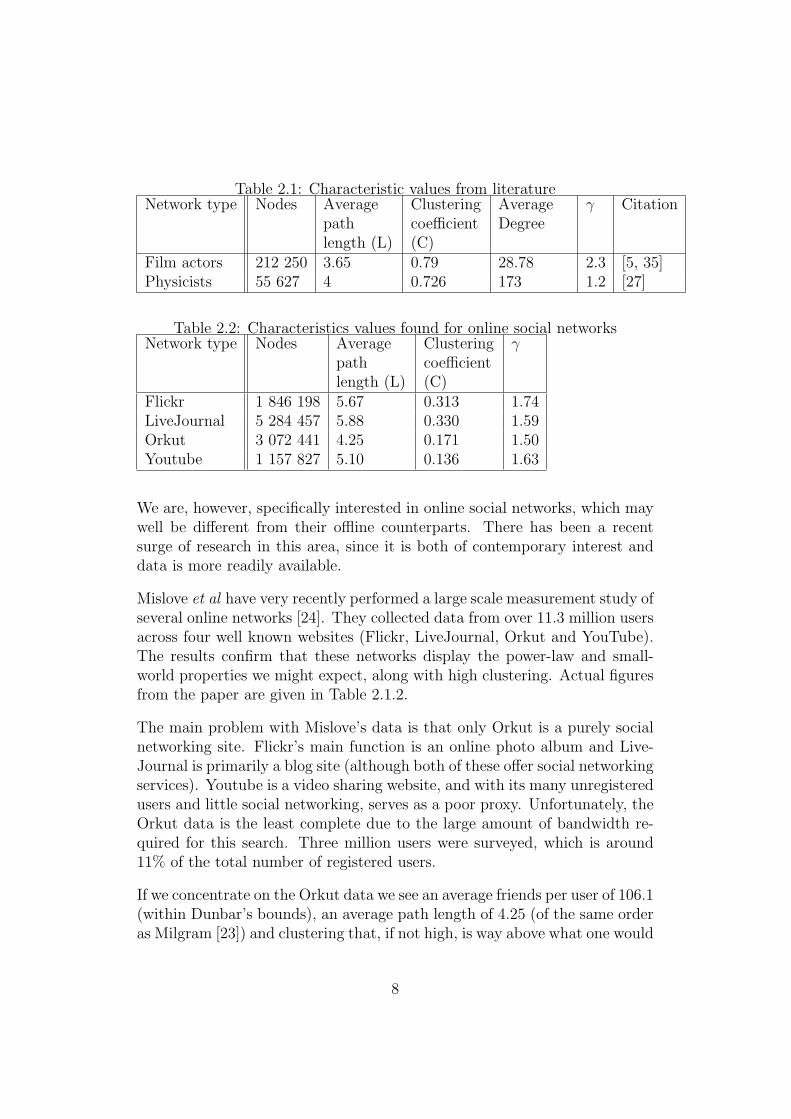
Table 2.1: Characteristic values from literatureNetwork type Nodes Average

pathlength (L)

Clusteringcoefficient(C)

AverageDegree

γ Citation

Film actors 212 250 3.65 0.79 28.78 2.3 [5, 35]Physicists 55 627 4 0.726 173 1.2 [27]

Table 2.2: Characteristics values found for online social networksNetwork type Nodes Average

pathlength (L)

Clusteringcoefficient(C)

γ

Flickr 1 846 198 5.67 0.313 1.74LiveJournal 5 284 457 5.88 0.330 1.59Orkut 3 072 441 4.25 0.171 1.50Youtube 1 157 827 5.10 0.136 1.63

We are, however, specifically interested in online social networks, which maywell be different from their offline counterparts. There has been a recentsurge of research in this area, since it is both of contemporary interest anddata is more readily available.

Mislove et al have very recently performed a large scale measurement study ofseveral online networks [24]. They collected data from over 11.3 million usersacross four well known websites (Flickr, LiveJournal, Orkut and YouTube).The results confirm that these networks display the power-law and small-world properties we might expect, along with high clustering. Actual figuresfrom the paper are given in Table 2.1.2.

The main problem with Mislove’s data is that only Orkut is a purely socialnetworking site. Flickr’s main function is an online photo album and Live-Journal is primarily a blog site (although both of these offer social networkingservices). Youtube is a video sharing website, and with its many unregisteredusers and little social networking, serves as a poor proxy. Unfortunately, theOrkut data is the least complete due to the large amount of bandwidth re-quired for this search. Three million users were surveyed, which is around11% of the total number of registered users.

If we concentrate on the Orkut data we see an average friends per user of 106.1(within Dunbar’s bounds), an average path length of 4.25 (of the same orderas Milgram [23]) and clustering that, if not high, is way above what one would

8

expect for a random graph. It also has a power law degree distribution, withγ ≈ 1.5, possibly indicating an underlying system of preferential attachment(see section 2.2.3).

2.2 Historical and Current Social Network Mod-

els

2.2.1 The Erdos and Renyi Random Network

Random graphs were initially developed within the bounds of pure math-ematics, with seminal work in the field coming from Erdos and Renyi [25].Despite this, it was the random network that first acted as a model of a socialnetwork for Pool and Kochen. We do not expect the random network to bea very realistic model, but it is a starting point.

A random network has two parameters: number of nodes, n, and probabilityof two nodes being connected, r. The type of social networks we are consid-ering will have large n and small r. If we know n and our required averagedegree, k, then r is simply

r =k

n

The average path length in a random network is small. It is by introducingsome randomness into a regular network that Watts and Strogatz were able toinduce the small world effect. The average path length in a random networkcan be calculated using

L =log n

log nr

[8]. Using characteristic values of n = 1000000, and r = 0.0001, we calculateL = 4, which is very low, and a bit lower than the eponymous six degrees ofseparation.

There is no clustering as such, since the probability that B and C are friendswith each other is, by definition of a random graph, independent from thefact that they both know A. In fact if we use the clustering coefficient asdefined in the previous section, it is simply equal to r for a truly randomnetwork. We are working with n = O(1000000) and k = O(100), which leadsto C = r ≈ 0.0001, this is of orders of magnitude less than the values intables 2.1.2 and 2.1.2.

9

All nodes in a random network have the same expected degree, therefore thedegree distribution certainly does not follow a power law. In fact

P (k) =

(n− 1k

)rk(1− r)n−1−k

which can be derived by considering the number of other nodes that are,(k),and are not, (n− 1− k), connected to our initial node. This is the binomialdistribution.

2.2.2 The Watts and Strogatz Small World Model

Watts and Strogatz set up their model by starting with a regular 1D ringnetwork with a given number of nodes, n, and degree of each node, k. Theythen introduced a third parameter, 0 ≤ q ≤ 1, where q is the probability thatan edge is ’rewired’ from its neighbour to another random node. Thereforeq = 0 is the original, regular network and q = 1 gives the fully rewirednetwork 2.

Watts and Strogatz observed that since small q affects only a very low per-centage of the nodes, the clustering coefficient remains largely unaffected.In contrast, average path length is significantly affected by the introductionof just a few ’shortcuts’, since these shortcuts have an impact, not only onthe path length between the newly connected nodes, but also between theirneighbours, and their neighours’ neighbours. It seems then, that a smallamount of rewiring has created the network we were looking for: low averagepath length and high clustering, in fact as n→∞, then infinitesimally smallq is sufficient to induce small world average path lengths [6].

Random rewiring does nothing to affect degree distribution, and consequentlythe Watts-Strogatz model still displays a binomial degree distribution.

2It should be noted that, because only one end of an edge is rewired with probabilityq, even q = 1 does not give a fully random network [6]. This has made analysis of thesystem difficult, and is one of the reasons that others have suggested modifications.

10

2.2.3 The Barabasi-Albert Model of Preferential At-tachment

In [5] Albert and Barabasi set out to examine the degree distribution ofa network modelled on preferential attachment. There network evolved asfollows.

The model takes n0 initial nodes and at each time step an action is performed:

• With probability 0 ≤ padd < 1, m ≤ m0 new edges are added. For eachnew link one node is chosen at random and connected to a second nodeselected with a probability

P (ki) =ki + 1∑j kj + 1

• With probability 0 ≤ prewire < 1− padd, m edges are ’rewired’. An edgeis selected at random and one of its ends moved to a new node, selectedpreferentially with probability P (ki) as above. This is done for each ofthe m edges.

• With probability 1−padd−prewire a new node is added, this node is givenm edges connected to existing nodes with the above defined probability,P (ki).

Since the aim of the model was to produce a power law degree distributionwe check this has been achieved.

Let ki be the degree of node i, then the probability that a new node willconnect to ki is

P (ki) =ki∑j kj

and therefore ki increases at a rate proportional to ki. In fact the rate ofgrowth is given by

dkidt

= mP (ki) =mki∑j kj

=ki2t

(2.1)

where m is the number of edges of the newly added node, and t is the timestep. If a node is added at each time step, the the total number of edges ismt, and hence ∑

j

kj = 2mt

11

since summing over all nodes counts each end of an edge. Therefore (2.1)becomes

dkidt

=ki2t

which can be solved to give

ki(t) = m(t

ti

) 12

(2.2)

where ti is the time at which node i was added. Therefore, if we wish tocalculate the probability that a node i has fewer connections that a set valuek, we may use (2.2), and rearrange

P (ki < k) = P

(m(t

ti

) 12

< k

)= P

(ti >

m2t

k2

)

which for equal time steps becomes

P

(ti >

m2t

k2

)= 1− P

(ti ≤

m2t

k2

)= 1− m2t

k2(t+m0)

The probability density function can be found via

pk =d(P (ki < k)

dk

which via (2.2.3) is

pk =2m2t

k3(t+m0)→ 2m2

k3for large t

We therefore see that modelling a network based on preferential attachmentproduces a power law degree distribution. This reflects real life as seen intables 2.1.2 and 2.1.2.

This model was setup with the intention of modelling the degree distributionand did not have the aim of modelling high clustering or short path-length.The authors do not mention these characteristics within their paper. Duringour matlab simulations the clustering coefficient can be calculated and wecan see how well this model represents this phenomenon.

12

2.2.4 The Davidsen Model of Introduction

This model is based around a simple premise: we often meet new friendsthrough our old friends. This basic assumption, along with the fact thatpeople join and leave a network, is enough to formulate the model.

All of the other models reviewed here are static models with fixed nodes andedges, whilst this makes them easier to study it is clearly an oversimplifica-tion. Dynamical models are at the forefront of current network research [28]but this model will be the only one consider within this report. In the nextsection we will look at value within a social network. It seems likely that thenetwork might grow in such a way as to optimise it’s value and therefore anetwork that grows organically as its value grows, seems to provide a betterbasis.

Taking a fixed number of nodes, n, with an initial number of edges betweenthem, we impose the following dynamics onto the system:

• A person is selected at random and two of their randomly selectedfriends are introduced, creating a new edge in the network if there wasnot already one in place. If the original person does not have enoughfriends to create an introduction, then they introduce themselves to astranger chosen at random.

• A person is chosen at random and, with probability q, they are removedfrom the network and all their edges are removed. A new person isintroduced to the network and given one, random, acquaintance.

The probability, q, gives us a time scale. In general, for a real social network,people are far less likely to die, or move away, than they are to meet newpeople, therefore a value of q � 1 will be considered. As this is our mainparameter (initial number of nodes and edges playing a less significant rolein a dynamic network that has reached steady state) it has an impact on thedegree distribution.

The preferential attachment built into this system comes from the fact thata person with many acquaintances has a increased probability of being se-lected to be introduced to a new person. The shape of the degree distributionchanges as we vary q, with a power law distribution for small p; the expo-nent being inversely related to q, (where the preferential linking dominates)through to an exponential degree distribution for large p. We would like

13

a model with a degree distribution that follows a power law, and we havediscussed above that small p is the more intuitive for social networks. Forq = 0.0025 we have

pk = k−1.35

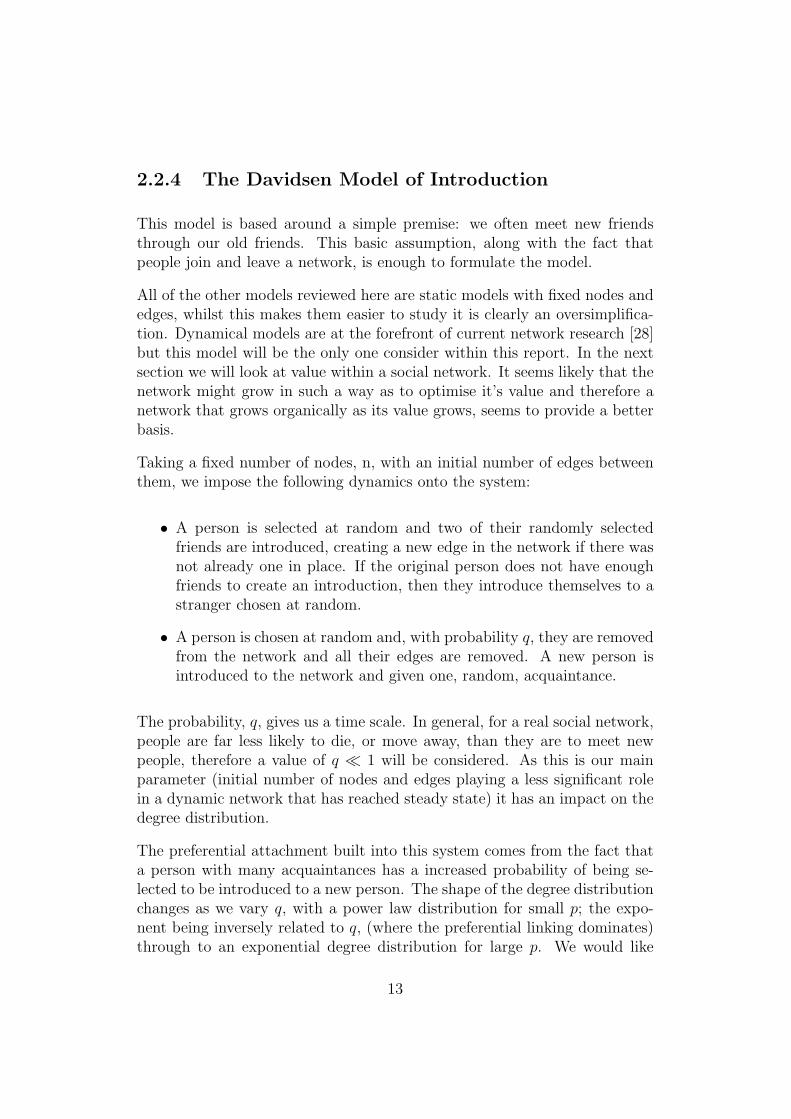
which fits in well with the values we see in table 2.1.2. There is a cutoff forlarge k due to the fact that the nodes have a limited lifetime and consequentlytheir number of acquaintances cannot grow without bound. This means ourdistribution is only a power-law up to a point; it does not have the long-tailthat we would otherwise expect. Figure 2.1 is the original graph from [9]showing both the power law regime and cutoff for large k.

Figure 2.1: The degree distribution pk of the model in statistically steadystate. For this graph n = 7000, although this does not have much affect.Original graph from [9].

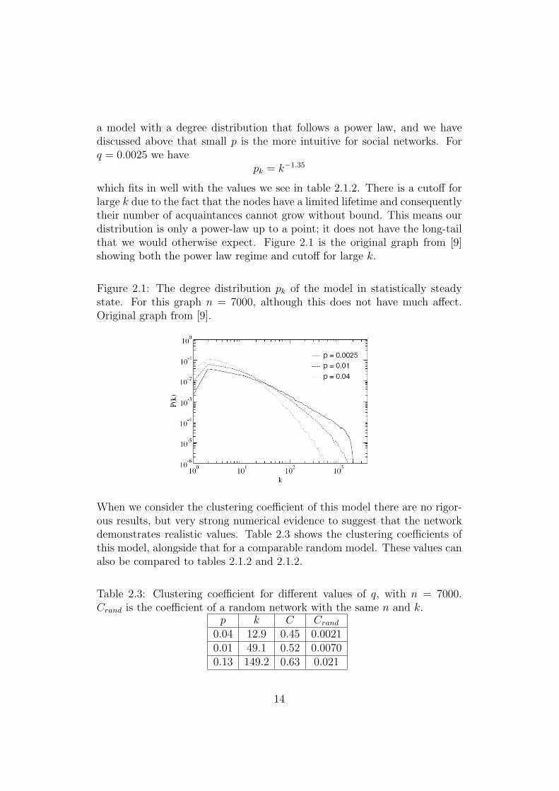
When we consider the clustering coefficient of this model there are no rigor-ous results, but very strong numerical evidence to suggest that the networkdemonstrates realistic values. Table 2.3 shows the clustering coefficients ofthis model, alongside that for a comparable random model. These values canalso be compared to tables 2.1.2 and 2.1.2.

Table 2.3: Clustering coefficient for different values of q, with n = 7000.Crand is the coefficient of a random network with the same n and k.

p k C Crand0.04 12.9 0.45 0.00210.01 49.1 0.52 0.00700.13 149.2 0.63 0.021

14

Average path length, L, can also be calculated for the network and is foundto be consistent with logarithmic behaviour, as required. For q = 0.0025 andn = 7000 we find that L = 2.38. This is higher than we would expect foran entirely random graph where Lrand = 1.77, and in fact a little lower thanwould be ideal.

15

Chapter 3

Calculating Value Growth

3.1 Theoretical Approaches to Value Growth

Not many people have looked at network value from an empirical researchperspective, but there are plenty of theoretical models in current circulation.Here we will review them.

3.1.1 Linear growth

Sarnoff’s Law

The value of a broadcast network grows linearly with the number of users.[32, 29]. This is a taken as fact for pure broadcast networks (e.g. televisionand radio) and we assume it is also true for broadcast websites (for examplenews based).

Linear growth in a communication network

There is some empirical evidence that linear growth might hold for commu-nication networks [30], despite the fact that it is counter-intuitive.

The two main theoretical arguments in support of this are based on conver-gent value distributions and consumption limits [37]. We have so far assumed

16

that each node derives equal value from each other node (many do [32, 33]),but this, of course, could be far from true. If the distribution value were tobe convergent, for example, if you valued connection with each node half asmuch as you did the last node, then the total value to any node would be

1 +1

2+

1

4+

1

8+ . . . =

∞∑x=1

1

2n→ 2

Therefore when we sum over all nodes we see a total value of 2n, i.e. O(n).We may now accept this or disregard it, but let us now cap the number ofconnections that are possible for each user (there are only so many hoursin the day), lets call this number C. Whilst the size of the network is stillgrowing below C then we will see quadratic growth (or some other typedependent on our value distribution), but once the cap is reached then eachnew user will instantly connect to the maximum number of people they wishto and network value will be, at most, nC, which is again O(n) since C isfixed.

3.1.2 Metcalfe’s Law

As mentioned briefly in the introduction, Metcalfe’s Law states that the valueof a communication network grows in proportion to the square of the numberof users [15]. The theory behind this is sound; the value of a communicationnetwork depends on communications, that is, interactions between users.The number of possible pairwise interactions in a network of n users is thenth triangle number, i.e. n(n−1)

2, which is clearly quadratic.

The devil is in the detail. Metcalfe’s original presentation was to try andencourage companies to install LANs with at least three machines [29, 33], hedid not say ’users’ he said ’compatibly communicating devices’. The problemcame when, during the dot-com boom, companies where keen to value theirnetworking businesses as highly as possible. They applied Metcalfe’s Lawwhere it did not belong. In a large network, not all the users are going tocommunicate with all the others - it is simply impossible in a network withmillions of users (which is the order we are talking about with online socialnetworks).

Another arguement against Metcalfe’s Law is put forward by Briscoe, Odlyzkoand Tilly [7, 29]. Their case is a logical one. If there is exist two networks,the first of size m and the second, n, then the values will be m2 and n2

respectively. If the two networks were to combine then the total value would

17

now be m2 + n2 + 2mn, and value has been gained ’for free’: it would beillogical for them not to merge. An important factor in this arguement is thevalue gained by each network is equal (mn); if one network were to profitmore than other from the deal, then this may cause a stale-mate, since thisis not the case then a merger must surely occur.

3.1.3 Reed’s Law

Any user of a social networking site will realise that they are not just aboutcommunicating with other people, but about communicating with groups ofother people. Despite Metcalfe’s Law seeming a bit ambitious, Reed arguesthan growth in some networks is even faster, in fact, it is exponential [32].

If a network supports the forming of groups then we consider how manygroups exist. The number of non-trivial subsets that can be formed in anetwork of size n is 2n − n− 1, which is clearly O(2n).

A key argument in Reed’s paper is that value can be derived from potentialconnectivity, rather than actual connectivity. This is a critical assumptionthat validates not only his findings, but Metcalfe’s Law too. Reed assumesthat each potential connection is worth as much as any other, which is simplynot borne out in real life since we have not seen exponential value growth inany network.

Reed’s Law is intuitively crazy. It does not seem at all feasible that a networkwith 101 people is worth double a network of 100 people, or the even moreextreme case that the birth of one child doubles the value of the world. Weuse the merger arguement again here [7]; if network value really did growexponentially then two separate networks would almost be forced to join up.

3.1.4 Zipf functions and Value as a Harmonic Series

A key assumption for Sarnoff, Metcalfe and Reed is that all connections areequally valuable. This simply isn’t true. In a large network most potentialconnections are never utilised [7], and this becomes obvious when one con-siders the network of the World Wide Web, where not everyone speaks thesame language.

Studies have shown that the number of interactions between two populations

18

is inversely proportional to the distance [29]. This is often called a ’gravitylaw’ since it is the same pattern as that of the gravitational attraction be-tween two masses. Specifically, if there are two populations, A and B ata distance d apart, then traffic is proportional to AB

dα , where α is a situa-tion dependent constant, usually between 1 and 2. If α = 2 (and that is acommon value for it to take in many real-life situations [37]) then the totalvalue is proportional to n log(n), for the details of this derivation please seeAppendix A.

Since we do not know what the distances are in an online network, indeed’distance’ may be defined in many ways, we try to derive the n log n valuevia alternative means.

We argued above that if the value distribution were convergent then overallgrowth would be linear. If the value is constant across all nodes we seeMetcalfe’s quadratic growth. We require something in between. Zipf’s Lawsays that if we order a large collection by popularity, the second on the listwill be worth about half of the first (in terms of whatever we are measuring)and the third on the list is worth one third the first, i.e. that the harmonicseries is generated [37]. In this case we do not have a convergent valuedistribution, rather a slowly diverging one,

1 +1

2+

1

3+

1

4+ . . . =

∞∑x=1

1

x

It is clear that this series diverges when we consider the integral test forconvergence. Since f(x) = 1

xis a non-negative monotone decreasing function

then the sum∑∞x=1

1x

converges if and only if the integral,∫∞x=1

1xdx is finite.

Since ∫ n

x=1

1

xdx = lnx|n1 = lnn− ln 1→∞as n→∞

then the integral is not finite and hence the sum diverges. It is a standardresult that the sum is bounded:

n∑1

1

k≤ lnn+ 1

please see Appendix B for a proof of this. This is the value for each of the nnodes, and hence the total value will be of order n log(n).

19

3.2 Empirical Research of Value Growth in a

Social Network

3.2.1 Dunbar’s Chistmas Card Questionnaire

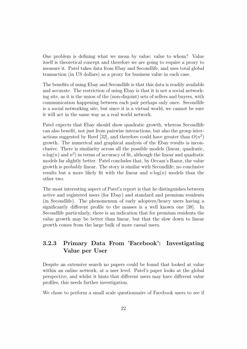
Data for actual social networks (as opposed to the proxies of citation andactor networks) is difficult to come by, especially when we become interestedin valuing these networks. The main reason being that it is difficult to collectthe data. Even if people are willing to sit down and tell you who all of theirfriends are, it is likely that they will forget some. It is even more likely thatnot all of those friends will be prepared to participate and hence the networkwill be largely incomplete. Recent approaches for estimating these networksizes have used smaller sub-populations to generate reliable figures, but areunable to provide information on value [22]. Psychologists Hill and Dunbarconducted a recent experiment to investigate this issue [11]. This paper usesthe exchange of Christmas cards and subjective questionnaire responses tovalue relationships. A graph from this paper, showing the distribution ofnetwork size across respondents, is reproduced in Figure 3.1. The meannetwork size is 153.5 (±84.5). This resonates well with previous work byDunbar [12], which uses human neocortex size to estimate a social group sizeof 150.

This paper also found further evidence to back Dunbar’s previous observa-tions that social networks are hierarchically different [11]. That is that onehas a core of very close friends and larger numbers of increasingly less intenserelationships. The previously published figures show clusterings of five (sup-port cliques), 12-15 (sympathy groups), 35 (bands) and 500 (mega bands).These figures have been verified by many others (for a list of references seethe bibliography for [11]).

3.2.2 Value Growth of an Online Social Network

The impetus for this project was the research paper by Shail Patel of Unilever[30]. Patel was interested to discover whether Metcalfe’s Law did indeedhold for a social network, and if it did not then what did hold. In his paperhis summarises the theoretical arguements and looks to empirical data forsupport. The use of empirical data to aid the understanding of network valuegrowth does not appear to have been tackled by others as of yet.

20

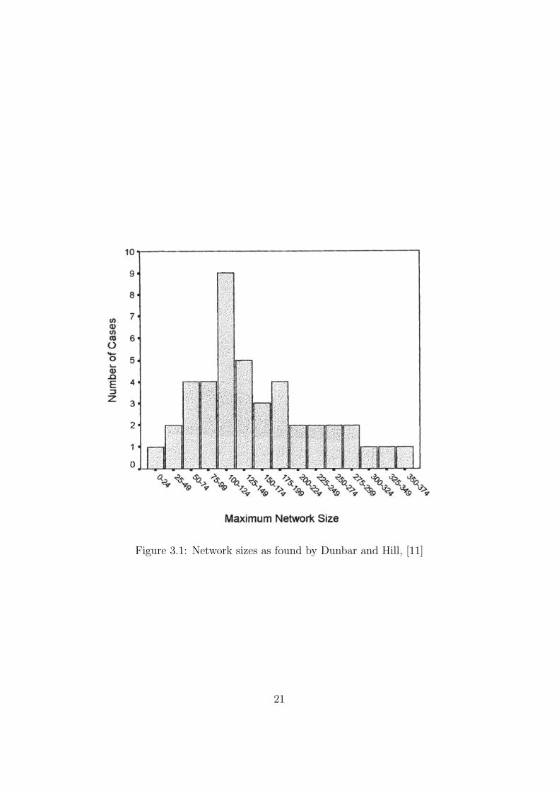
Figure 3.1: Network sizes as found by Dunbar and Hill, [11]

21

One problem is defining what we mean by value; value to whom? Valueitself is theoretical concept and therefore we are going to require a proxy tomeasure it. Patel takes data from Ebay and Secondlife, and uses total globaltransaction (in US dollars) as a proxy for business value in each case.

The benefits of using Ebay and Secondlife is that this data is readily availableand accurate. The restriction of using Ebay is that it is not a social network-ing site, as it is the union of the (non-disjoint) sets of sellers and buyers, withcommunication happening between each pair perhaps only once. Secondlifeis a social networking site, but since it is a virtual world, we cannot be sureit will act in the same way as a real world network.

Patel expects that Ebay should show quadratic growth, whereas Secondlifecan also benefit, not just from pairwise interactions, but also the group inter-actions suggested by Reed [32], and therefore could have greater than O(n2)growth. The numerical and graphical analysis of the Ebay results is incon-clusive. There is similarity across all the possible models (linear, quadratic,n log(n) and n2) in terms of accuracy of fit, although the linear and quadraticmodels far slightly better. Patel concludes that, by Occam’s Razor, the valuegrowth is probably linear. The story is similar with Secondlife; no conclusiveresults but a more likely fit with the linear and n log(n) models than theother two.

The most interesting aspect of Patel’s report is that he distinguishes betweenactive and registered users (for Ebay) and standard and premium residents(in Secondlife). The phenomenum of early adopters/heavy users having asignificantly different profile to the masses is a well known one [38]. InSecondlife particularly, there is an indication that for premium residents thevalue growth may be better than linear, but that the slow down to lineargrowth comes from the large bulk of more casual users.

3.2.3 Primary Data From ’Facebook’: InvestigatingValue per User

Despite an extensive search no papers could be found that looked at valuewithin an online network, at a user level. Patel’s paper looks at the globalperspective, and whilst it hints that different users may have different valueprofiles, this needs further investigation.

We chose to perform a small scale questionnaire of Facebook users to see if

22

we could learn anything from data on a user level.

This time the proxy for value to a user is the amount of time they spendonline. It is value to a user in the sense that that is the value they place onthe network. It can be translated into value to the network (or at least valueto the business) as a user with more hours online will provide more eyeballs interms of advertising - there are standard techniques used in market researchto convert social value into a financial amount [37].

The main critic

There are clearly huge drawbacks with the data. The three main factorsbeing sample size, sample selection and self-reporting errors. The samplesize is very, very small, only 45 data points are used, whereas Facebook hasa network size of over 90 million active users. Whilst many would arguethat this is a pointlessly small sample, these are only initial findings andwe would encourage others to follow this up. The sample is not random, inthat all the invited people are this author’s Facebook friends 1. This clearlynarrows the field to a small demographic, although in terms of age and sexthe sample is broadly representative of Facebook as a whole [13]. Since thequestionnaire is a voluntary one, perhaps the sample is biased because of thepeople who chose to partake. Finally we have the problem of self-reporting.The number of friends a user has is a factual statistic, whereas number ofhours spent online is volunteered information. We expected under-reportingof this value, as people tend to be embarrassed at high usage levels. We triedto minimize this by making the questionnaire as anonymous as possible. Inthe end most people chose to share their data publically and under-reportingdoes not appear to be a problem as the figures are, if anything, higher thanexpected.

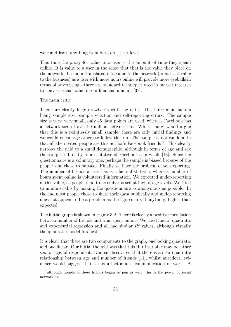
The initial graph is shown in Figure 3.2. There is clearly a positive correlationbetween number of friends and time spent online. We tried linear, quadraticand exponential regression and all had similar R2 values, although visuallythe quadratic model fits best.

It is clear, that there are two components to the graph, one looking quadraticand one linear. Our initial thought was that this third variable may be eithersex, or age, of respondent. Dunbar discovered that there is a near quadraticrelationship between age and number of friends [11], whilst anecdotal evi-dence would suggest that sex is a factor in a communication network. A

1although friends of these friends began to join as well: this is the power of socialnetworking!

23

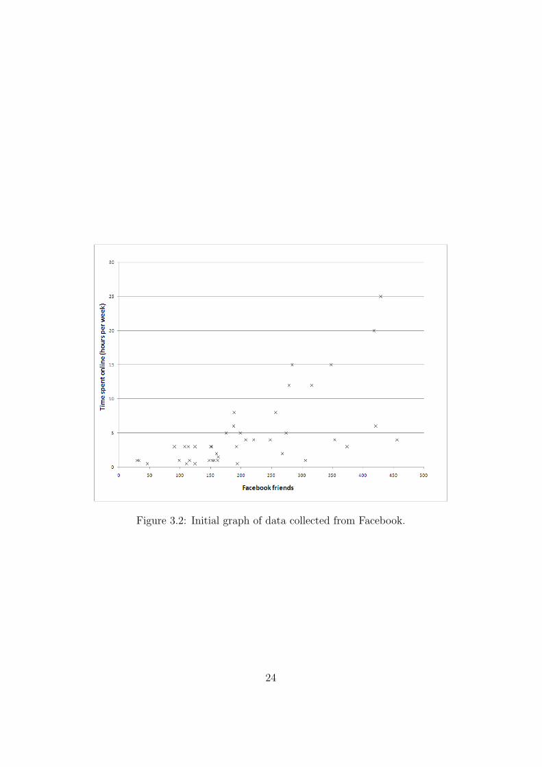
Figure 3.2: Initial graph of data collected from Facebook.

24

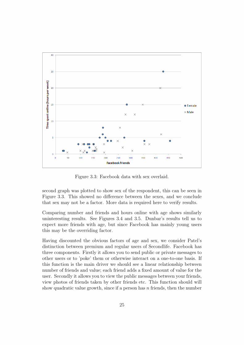
Figure 3.3: Facebook data with sex overlaid.

second graph was plotted to show sex of the respondent, this can be seen inFigure 3.3. This showed no difference between the sexes, and we concludethat sex may not be a factor. More data is required here to verify results.

Comparing number and friends and hours online with age shows similarlyuninteresting results. See Figures 3.4 and 3.5. Dunbar’s results tell us toexpect more friends with age, but since Facebook has mainly young usersthis may be the overriding factor.

Having discounted the obvious factors of age and sex, we consider Patel’sdistinction between premium and regular users of Secondlife. Facebook hasthree components. Firstly it allows you to send public or private messages toother users or to ’poke’ them or otherwise interact on a one-to-one basis. Ifthis function is the main driver we should see a linear relationship betweennumber of friends and value; each friend adds a fixed amount of value for theuser. Secondly it allows you to view the public messages between your friends,view photos of friends taken by other friends etc. This function should willshow quadratic value growth, since if a person has n friends, then the number

25

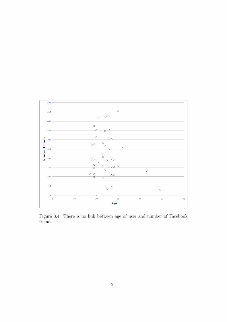
Figure 3.4: There is no link between age of user and number of Facebookfriends.

26

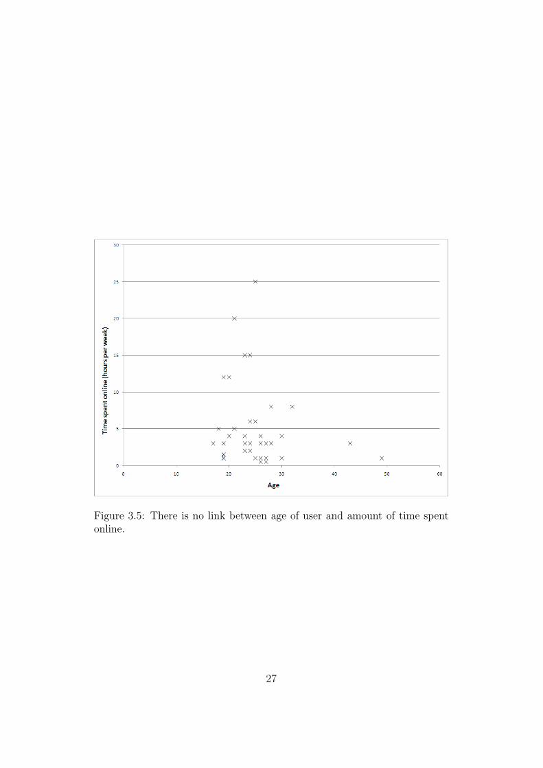
Figure 3.5: There is no link between age of user and amount of time spentonline.

27

of ’interconnections’ they may view will be O(12n(n− 1)) and hence as they

add friends to their list, value of the service will grow quadratically. Thirdlyit allows you to create and join groups, and communicate with the membersof that group, it is possible that where we will see exponential growth assuggested by Reed [32].

It is important to note here that this linear/quadratic/exponential growth isnot in relation to the size of the entire network, only in relation to the size ofan individual’s personal network. The implications of this will be discussedfurther in Section 3.3.

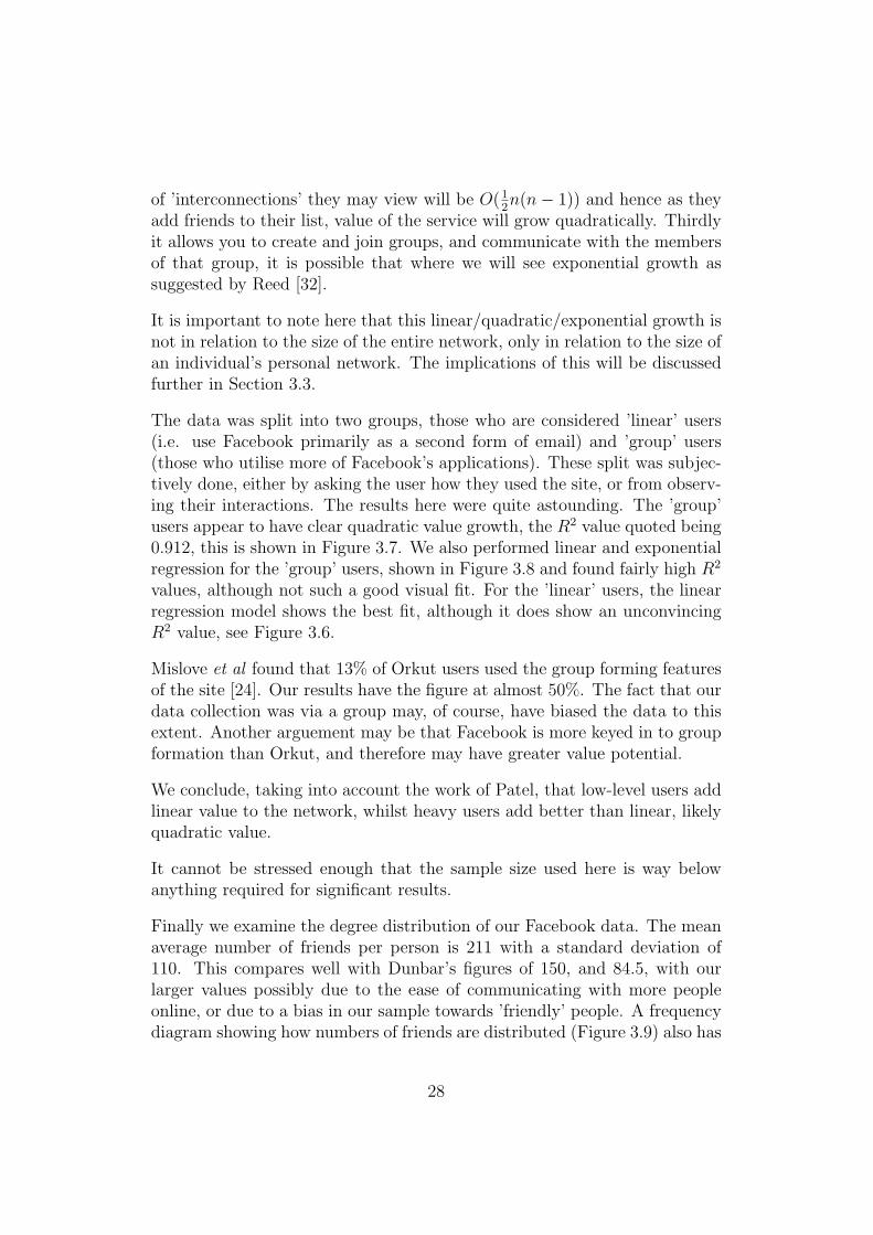
The data was split into two groups, those who are considered ’linear’ users(i.e. use Facebook primarily as a second form of email) and ’group’ users(those who utilise more of Facebook’s applications). These split was subjec-tively done, either by asking the user how they used the site, or from observ-ing their interactions. The results here were quite astounding. The ’group’users appear to have clear quadratic value growth, the R2 value quoted being0.912, this is shown in Figure 3.7. We also performed linear and exponentialregression for the ’group’ users, shown in Figure 3.8 and found fairly high R2

values, although not such a good visual fit. For the ’linear’ users, the linearregression model shows the best fit, although it does show an unconvincingR2 value, see Figure 3.6.

Mislove et al found that 13% of Orkut users used the group forming featuresof the site [24]. Our results have the figure at almost 50%. The fact that ourdata collection was via a group may, of course, have biased the data to thisextent. Another arguement may be that Facebook is more keyed in to groupformation than Orkut, and therefore may have greater value potential.

We conclude, taking into account the work of Patel, that low-level users addlinear value to the network, whilst heavy users add better than linear, likelyquadratic value.

It cannot be stressed enough that the sample size used here is way belowanything required for significant results.

Finally we examine the degree distribution of our Facebook data. The meanaverage number of friends per person is 211 with a standard deviation of110. This compares well with Dunbar’s figures of 150, and 84.5, with ourlarger values possibly due to the ease of communicating with more peopleonline, or due to a bias in our sample towards ’friendly’ people. A frequencydiagram showing how numbers of friends are distributed (Figure 3.9) also has

28

Figure 3.6: ’Linear users’ show linear friends/value relationship

29

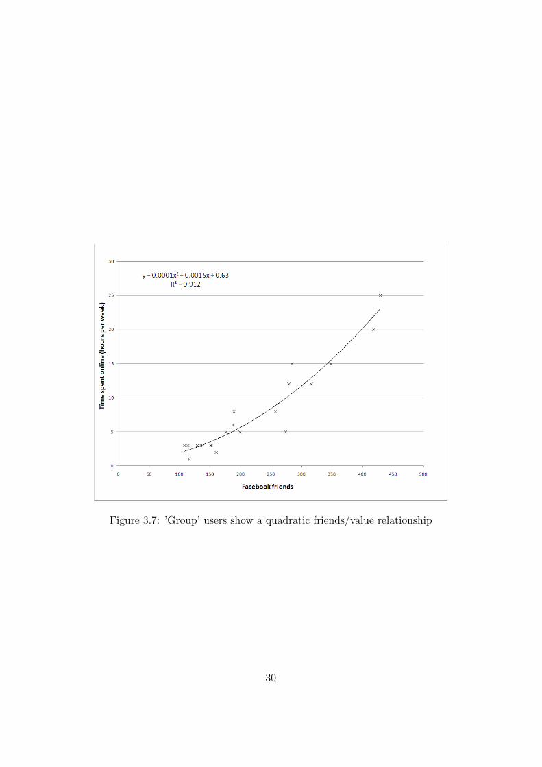
Figure 3.7: ’Group’ users show a quadratic friends/value relationship

30

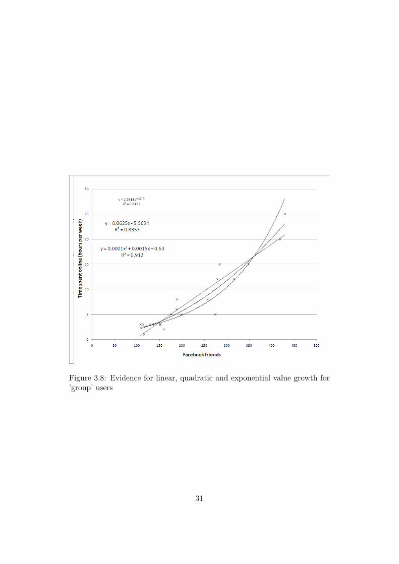
Figure 3.8: Evidence for linear, quadratic and exponential value growth for’group’ users

31

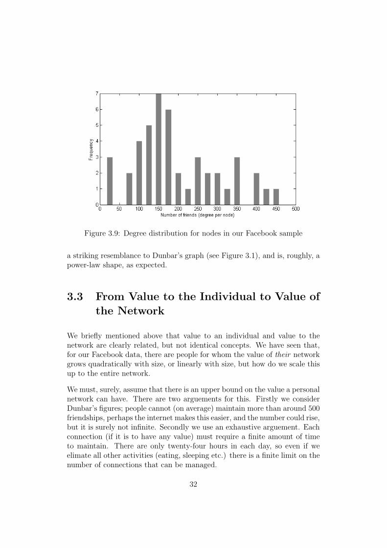
Figure 3.9: Degree distribution for nodes in our Facebook sample

a striking resemblance to Dunbar’s graph (see Figure 3.1), and is, roughly, apower-law shape, as expected.

3.3 From Value to the Individual to Value of

the Network

We briefly mentioned above that value to an individual and value to thenetwork are clearly related, but not identical concepts. We have seen that,for our Facebook data, there are people for whom the value of their networkgrows quadratically with size, or linearly with size, but how do we scale thisup to the entire network.

We must, surely, assume that there is an upper bound on the value a personalnetwork can have. There are two arguements for this. Firstly we considerDunbar’s figures; people cannot (on average) maintain more than around 500friendships, perhaps the internet makes this easier, and the number could rise,but it is surely not infinite. Secondly we use an exhaustive arguement. Eachconnection (if it is to have any value) must require a finite amount of timeto maintain. There are only twenty-four hours in each day, so even if weelimate all other activities (eating, sleeping etc.) there is a finite limit on thenumber of connections that can be managed.

32

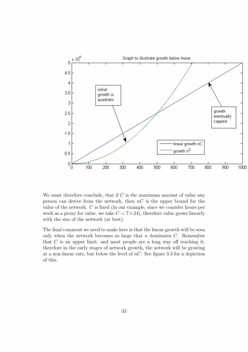
We must therefore conclude, that if C is the maximum amount of value anyperson can derive from the network, then nC is the upper bound for thevalue of the network. C is fixed (in our example, since we consider hours perweek as a proxy for value, we take C = 7×24), therefore value grows linearlywith the size of the network (at best).

The final comment we need to make here is that the linear growth will be seenonly when the network becomes so large that n dominates C. Rememberthat C is an upper limit, and most people are a long way off reaching it,therefore in the early stages of network growth, the network will be growingat a non-linear rate, but below the level of nC. See figure 3.3 for a depictionof this.

33

Chapter 4

Developing A Model

In order to measure value growth within a social network it was importantto both build a model of the network and create a means of valuing. Webegan by developing Matlab models of each of the four models discussed inSection 2.2. The coding for each of these can be found in Appendix C.

Each model consists of A, an n× n matrix, with friendship between nodes iand j being created by a non-zero value in A(i, j). The precise value of A(i, j)is indicative of the value that i places upon j, and as such is not necessarilyreciprocal (in fact it rarely is and in some cases A(i, j) 6= 0, A(j, i) = 0).The maximum value any node can place on any other is 1, with others beinga fraction of this. To calculate the total network value we sum across allindividual node values. The impact of this is that a model with equal valueacross all nodes will always have greater value than one with, for example,a Zipf value profile. Since we are only interested in the shape of the growthhowever, this is unimportant to us.

To value these networks we developed four value profiles which could be usedwith each of the four networks. The four value profiles are

• Equal value weighting each connection is valued at 1

• Truncated assuming there is a limit to the number of friendships thatcan be maintained, a certain number of connections are valued at 1 andafter this no more connections can be made

• Zipf value the first connection a node makes is valued at 1, the secondat 1

2, the nth at 1

n

34

• Truncated Zipf value as for Zipf, but assuming there is a limit to thenumber of friendships

• Dunbar value following on from Dunbar’s work, different groups aregiven different values, with value decreasing as group size increases

4.1 Verifying Existing Results

We realised early on that the Small World model has identical value proper-ties to the random model since average path length does not affect the valuewithin the network. Whilst it was felt that, in fact, connecting to a nodethat created short path lengths would be a potentially beneficial move foranother node, and hence one that could be highly valued, there are two issuesto consider. Firstly there is no data to support this hypothesis. Secondly,the calculation of average path length within Matlab was far too calculationheavy and could not even be implemented once, never mind at each iterationto facilitate connection choices. For this reason the Small Word network doesnot feature in any analysis.

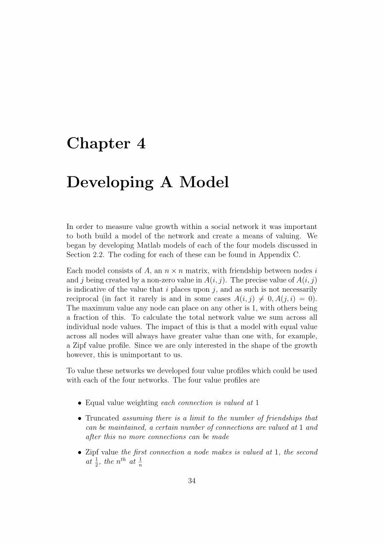
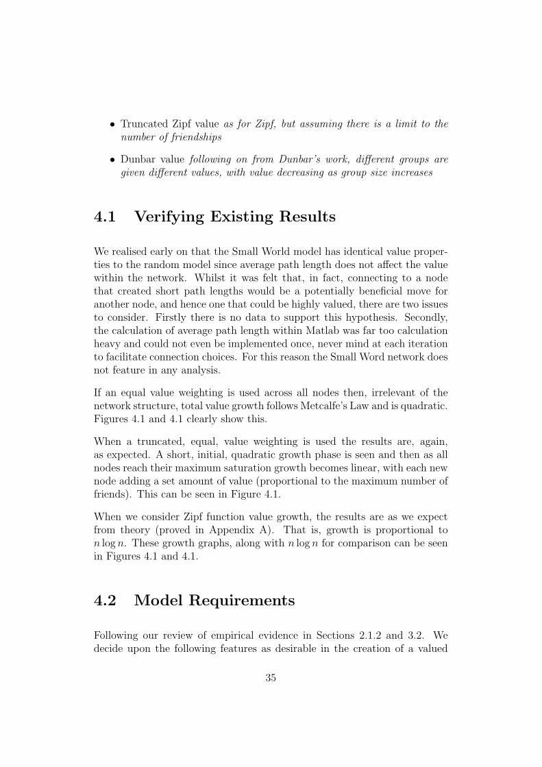
If an equal value weighting is used across all nodes then, irrelevant of thenetwork structure, total value growth follows Metcalfe’s Law and is quadratic.Figures 4.1 and 4.1 clearly show this.

When a truncated, equal, value weighting is used the results are, again,as expected. A short, initial, quadratic growth phase is seen and then as allnodes reach their maximum saturation growth becomes linear, with each newnode adding a set amount of value (proportional to the maximum number offriends). This can be seen in Figure 4.1.

When we consider Zipf function value growth, the results are as we expectfrom theory (proved in Appendix A). That is, growth is proportional ton log n. These growth graphs, along with n log n for comparison can be seenin Figures 4.1 and 4.1.

4.2 Model Requirements

Following our review of empirical evidence in Sections 2.1.2 and 3.2. Wedecide upon the following features as desirable in the creation of a valued

35

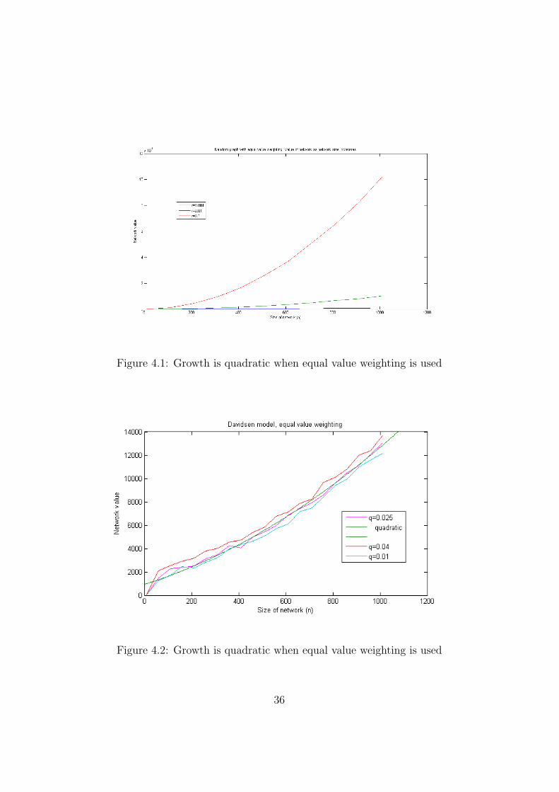
Figure 4.1: Growth is quadratic when equal value weighting is used

Figure 4.2: Growth is quadratic when equal value weighting is used

36

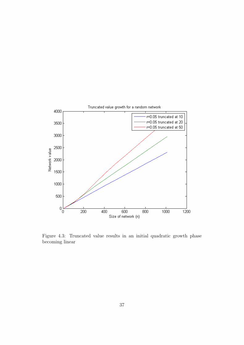
Figure 4.3: Truncated value results in an initial quadratic growth phasebecoming linear

37

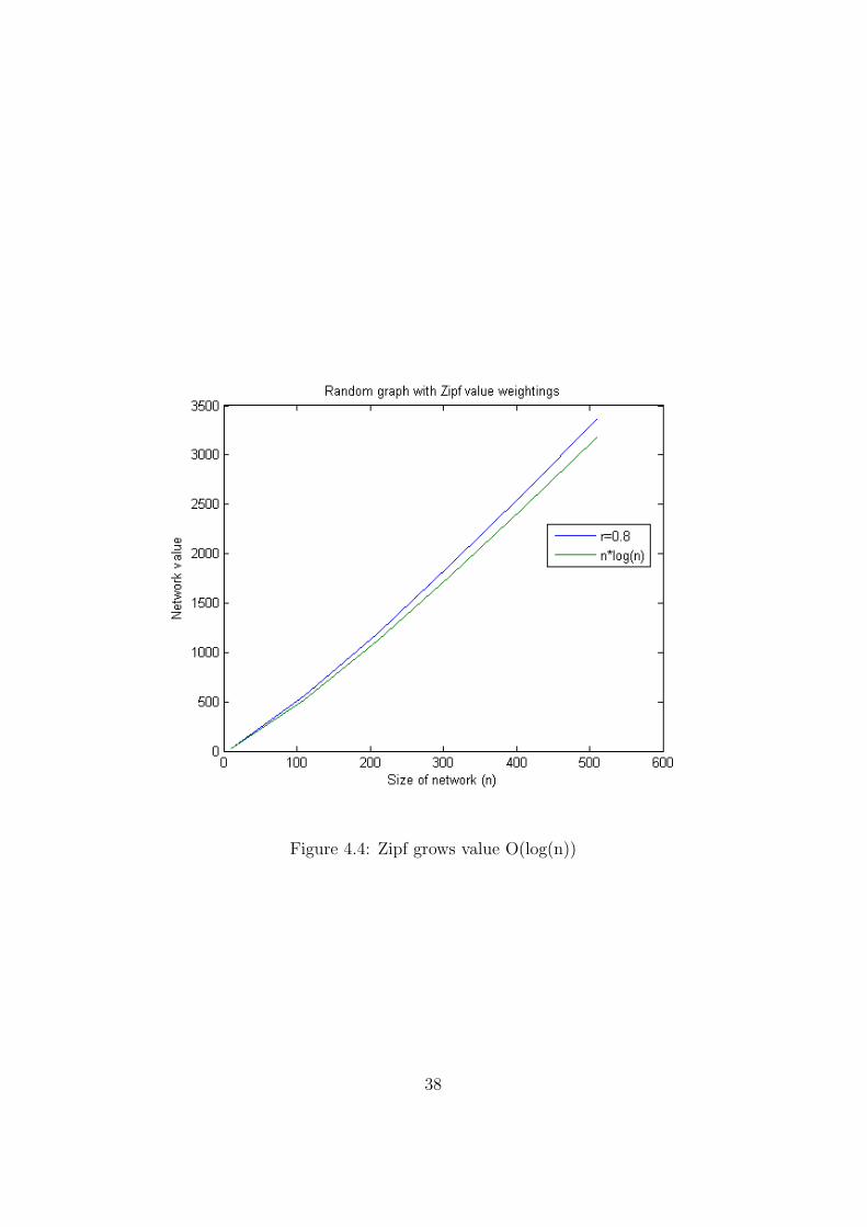
Figure 4.4: Zipf grows value O(log(n))

38

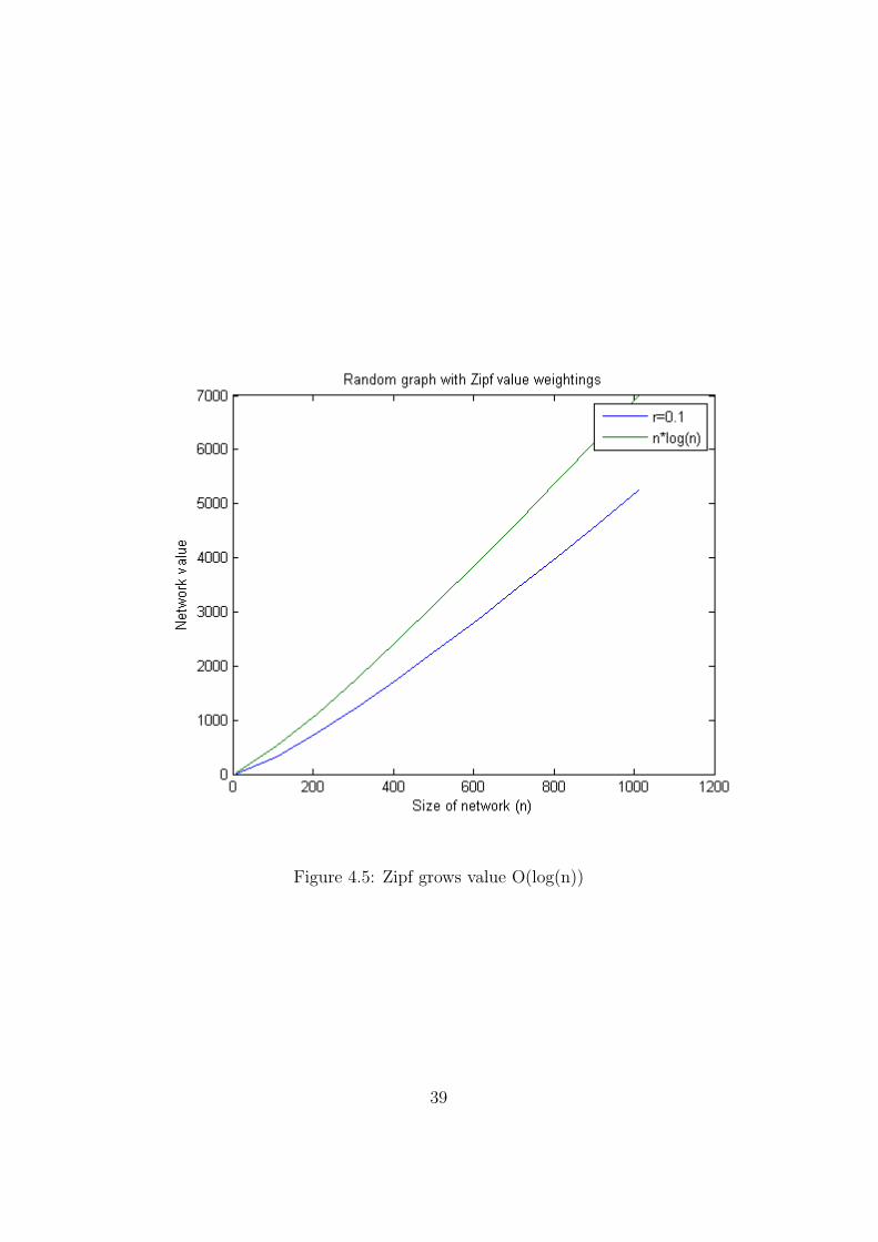
Figure 4.5: Zipf grows value O(log(n))

39

social network model.

• A large number of nodes (ideally O(106), although this will be impos-sible on Matlab)

• An average number of friends of between,approximately, 100 and 150

• A power law degree distribution with an exponent of around γ = 1.5.

• A clustering coefficient of approximately 0.3, and certainly higher thanthat expected at random

• Short average path-lengths of around 5

• A value profile that distinguishes between different levels of friendship(from Dunbar’s groupings), truncated at 500 connections per user

• A value profile that distinguishes between two types of users, witharound one half deriving value from direct connections only and theother half also finding value in connections between friends

4.3 Final Model

For the final model we elected to use Davidsen’s model. This was chosen forseveral reasons.

Firstly it is a dynamic model. Since we are measuring value growth, thisis considered an important factor. To measure the growth of all the staticmodels, many different sized models were created and valued. Whilst thisgives a good indication of how value varies with size it isn’t quite the sameas an actual ’growing’ network.

Secondly it offers us a power law degree distribution. The final model usesq = 0.0025, which results in γ ≈ 1.35, which is close to the required 1.5.

It also, for q = 0.0025, offers us an average degree of 149.2 [9], which fitsperfectly with our requirements.

Thirdly it provides high clustering. The clustering coefficient for q = 0.0025and N = 7000 is quoted in [9] as 0.63.

40

Fourthly, average path lengths are too expensive to calculate on Matlab, butDavidsen quotes a value of l = 2.38, which, whilst shorter than observed,is still of a similar order, and does, at least, demonstrate the ’small world’nature we would like to see.

It is the high clustering and low path lengths that made the Davidsen ourmodel of choice above the Barabasi-Albert model (which is dynamic and hasa power law degree distribution).

Our Davidsen model requires four inputs, n, q, r and maxtime. The matrixdimension, n determines the maximum number of people within the network,although since the network is growing dynamically not all of these are ’live’.We calculate the actual size of the network at any given time by findingthe number of nodes of non-zero degree. The probability q gives our modela time scale, it is the probability that, at each timestep, a node will bedeleted. This was the main parameter that needed adjusting as it affectedthe degree distribution of the model. In the final model we found that theinput value r (used as the probability of connection in the initial setup ofa random network) had little effect, except when r >> 0 in which case therandom graph dominated the preferential attachment model. For this reasonwe set r = 0. Therefore at timestep one the matrix is empty and there are noconnections, and the network grows from here. Finally we consider maxtime.This is the number of iterations through which the model will run.

Initially we attempted to use the value distribution based directly on Dun-bar’s observed group sizes, but there were two main drawbacks. Firstly itproved difficult to decide on precise values for each group level (Dunbar givesus none). Secondly because we were unable to attain large enough networksizes (due to restrictions in computing power), average numbers of friendsare stuck at around 30. Dunbar’s figures require many more friends than thisand it was unclear how to scale down the group sized accordingly. It wasconcluded that a Zipf function showed many similarities to Dunbar’s figuresand that, in fact, Dunbar’s empirical figures are quite likely an approxima-tion of a underlying Zipf distribution. We therefore grow value in accordancewith Zipf.

To distinguish between the two types of user we split the network into two.This was implemented in two separate ways. Initially we set all even num-bered nodes to be of the linear/email user type and odd nodes to be groupusers. After some thought we realised that, as suggested by Patel [30], it ismost likely the early adopters who will have higher usage levels. We thereforeadapted the model so that the first fifty percent of users are of the group use

41

type, and the second half are the more casual email users.

When calculating the value of the network to a ’linear’ user, i, we simplysummed along the ith row, where the values A(i, j) indicate the value thati places upon j. Since the valuations were made using a Zipf function thisapproximates to log n. For the ’quadratic users’ we initially sum the indi-vidual valuations as we did for linear users. To calculate the value to i oftwo friends communicating with each other we firstly need to know if thesetwo friends of i are indeed friends with each other. This proved too calcu-lation heavy, and we decided to approx the situation by assuming that allfriends were mutual. Whilst this is far from being true, with such a highclustering coefficient, it is not too far fetched either. To calculate the thirdparty connection we calculated A(i, j) × A(i, k) to find the value to i of jand k communicating with each other. This values connections between twovalued friends more highly than connections between those less important,which fits with qualitative opinions of Facebook’s users on this matter.

Despite the fact that a large network was at the top of our list of criteria,N = O(106) was never going to be achieved with our matrix setup on Matlab.We found that N = O(103) was achievable, which in fact, is all that Davidsenet al worked with in [9]. It appears that modelling large enough networks isa universal problem.

42

Chapter 5

Conclusions

5.1 Results of the Model

The amount of calculation and memory required to handle the matriceswithin Matlab, even utilising the sparse matrix setup, has restricted us tonetworks with N = 600 and 10000 iterations of the growth cycle. This hadhuge implications for us regarding the upper limit on the number of friends,which was set, from Dunbar’s figures, at 500. The average number of friendsper user remained at around 3, and hence the cap was useless. Figure 5.1shows the degree distribution for this case. This meant that with the cap inplace we were seeing greater than quadratic growth. See Figure 5.1 to seethis.

Enlarging the network was not possible, and therefore, in an attempt to seemore realistic results, we reduced the cap. Unfortuanately, due to the size ofthe required networks, we could not get any results worth printing. With acap of one in place, growth is linear, but this result is trivial, since if eachperson in a network can have only one friend, of course growth will growlinearly (no interactions are possible between mutuall friends either). Evenwith a cap of just two, we could not grow a large enough network.

Whilst it is very disappointing that no graphical or numeric results couldbe produced, we still believe that this research suggests that networks gothrough an initial phase of fast value growth, better than quadratic, beforeall users become saturated and then growth continues linearly. This is in factthe opposite of Metcalfe’s Law (which implied that growth may start slowly

43

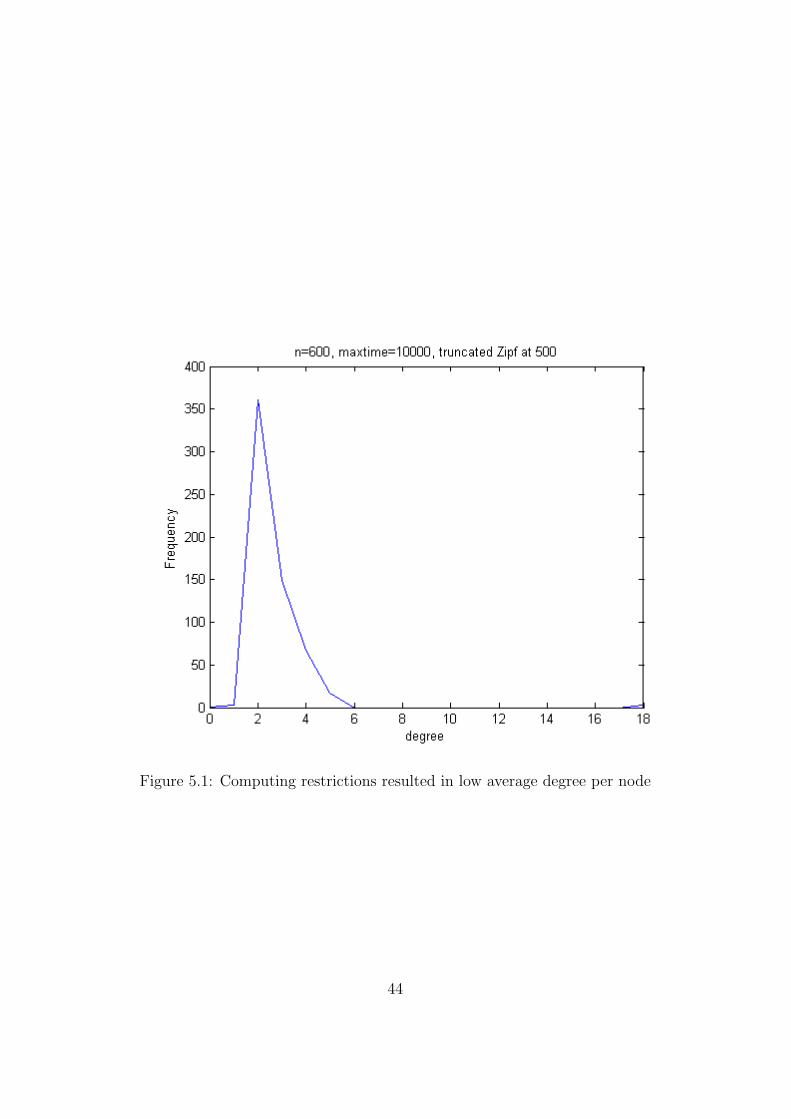
Figure 5.1: Computing restrictions resulted in low average degree per node

44

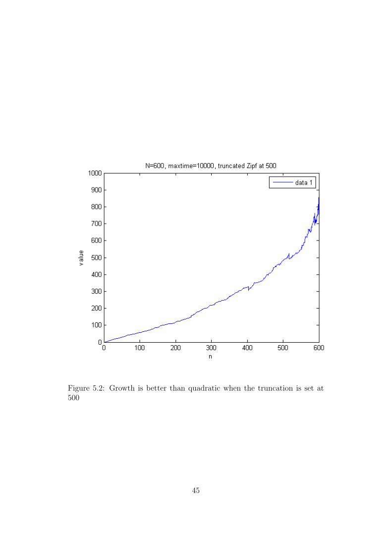
Figure 5.2: Growth is better than quadratic when the truncation is set at500

45

and then would become quadratic once a certain critical mass was achieved).

The question is, when is this point reached in real online social networks?We were not able to achieve realistic values due to computing constraints, itwould be interesting to try this model on a more powerful machine.

Whilst our results are far from conclusive, we do not believe that Metcalfe’sLaw is valid for online social networks.

5.2 Review of the Model and Suggestions for

Further Work

This project has thrown up far more questions that it has managed to answer.

We feel that the most exciting idea, worthy of further consideration, is thatof the two (or quite possibly more) user types within a network behaving dif-ferently in their approaches to valuing the network. We split our Facebookusers into ’email’ and ’group’ types, although it is immediately clear thatthree types of communicators (one-to-one, those interested in the communi-cation of others, and group users) may have been more appropriate. It is, ofcourse, possible that people move between different types of usage, and thiscould be factored in as well.

The very small sample size for the Facebook analysis, along with the manypossible biases in the sample, is an obvious issue and could certainly beaddressed in a larger survey. Intrinsically, any questionnaire of this naturewill attract more heavy users which will bias the data. Mislove et al [24]got around this problem very well in their survey with screen scraping thedata. It would be simple to find a users number of friends, age and sex usingthis method, in addition, Facebook pages do contain the information abouta users current online/offline status, and whilst massively time-consuming itwould be possible to collect the hours online data in this way too. The usertype was, as discussed, a subjective decision on either their part, or ours. Itwould be possible to put stricter definitions on this, to avoid any bias here.

This report uses data from Dunbar’s investigation of social group sizes [11].It is not known how relevant this data is to online social groups. We wouldexpect a certain, probably large, amount of similarity, but it would be inter-esting to see similar surveys being conducted of online friendships. The data

46

would be easier to find online, and it seems likely, with current interest inonline networking, that this research will appear soon.

47

Bibliography

[1] Albert and Barabasi, Topology of Evolving Networks: Local Events andUniversality, Physical Review Letters, 85, 2000, 5234–5237

[2] Amaral, Scala, Barthelemy and Stanley, Classes of small-world networksPNAS, 97, 2000, 11149–11152

[3] Arthur, Increasing Returns and the New World of Business, HarvardBusiness Review, July 1996

[4] Backstrom, Huttenlocher, Kleinberg and Lan, Group Formation in LargeSocial Networks: Membership, Growth and Evolution, KDD, ’06, 2006,August 20–23

[5] Barabasi and Albert, Emergence of Scaling in Random Networks, Sci-ence, 286, 1999, 509–512

[6] Barrat and Weigt, On the properties of small-world network models,European Physical Journal B, 13, 2000, 547–560

[7] Briscoe, Odlyzko and Tilly Metcalfe’s Law is Wrong, IEEE Spectrum,2006, 26–31

[8] Chung and Lu, Complex Graphs and Networks, CBMS, 2004

[9] Davidson, Ebel and Bornholdt, Emergence of a Small World from LocalInteractions: Modeling Acquaintance Networks, Physical Review Let-ters, 88, 2002, 128701-1–4

[10] Dorogovtsev, Mendes and Samukhin, Structure of Growing Networkswith Preferential Linking Physical Review Letters, 85, 2000, 4633–4636

[11] Dunbar and Hill, Social network size in humans Human Nature, 14,2002, 53–72

48

[12] Dunbar, Coevolution of Neocortical Size, Group Size and Language inHumans, Behavioural and Brain Sciences, 16, 1993, 681–735

[13] Facebook, http://www.new.facebook.com/press/info.php?statistics

[14] Fichman, Information Technology Diffusion: A Review of Empirical Re-search, Proceedings of the International Conference of Information Sys-tems, 13, 1992, 195

[15] Gilder, Metcalfe’s Law and Legacy, Forbes, September 1993

[16] Grossman, The Business Value of Social Networking, Forbes, July 2008

[17] Goyal, Connections, Princeton UP

[18] Holme and Newman, Nonequilibrium phase transition in the coevolutionof networks and opinions Phys. Rev. E 74, 2006

[19] Lauria, MySpace Loves Facebook Value, New York Post, 26 October 2007

[20] Liebowitz and Margolis, Network Externalities (Effects), The New Pal-graves Dictionary of Economics and the Law, MacMillan, 1998

[21] Leskovec, Singh and Kleinberg, Patterns of Influence in a Recommen-dation Network,

[22] McCarty, Killworth, Bernard, Johnson and Shelley, Comparing twomethods for estimating network size, Human Organization 60, 2001,28–39

[23] Milgram, The Small World Problem, Psychology Today, 2, 1967, 60–67

[24] Mislove, Marcon, Gummadi, Druschel and Bhattacharjee, Measurementand Analysis of Online Social Networks, IMC ’07: Proceedings of the7th ACM SIGCOMM conference on Internet measurement, 2007, 29–42

[25] Newman, Watts and Strogatz, Random graph models of social networks,PNAS, 99, 2002, 2566–2572

[26] Newman, The Structure and Function of Complex Networks, SIAM Re-view, 45, 2003, 167–256

[27] Newman, Strogatz and Watts, Random graphs with arbitrary degree dis-trubutions and their applications, Physical Review E 64, 2001,

49

[28] Newman, Barabasi and Watts, The Structure and Dynamics of Net-works, Princeton UP, 2006

[29] Odlyzko and Tilly, A refutation of Metcalfe’s Law and a net-ter estimate for the value of networks and network connections,www.dtc.umn.edu/ odlyzko/doc/metcalfe.pdf

[30] Patel, Report on Value Within A Communication Network, Confidentialinternal Unilever document, 2007

[31] Pool and Kochen, Contacts and Influence, Social Networks 1, 1978, 1–48

[32] Reed, That Sneaky Exponential - Beyond Metcalfe’s Law to the Powerof Community Building, Context, 1999

[33] Simeonov, Metcalfe’s Law: more misunderstood than wrong?,2006, http://simeons.wordpress.com/2006/07/26/metcalfes-law-more-misunderstood-than-wrong/

[34] Vega-Redondo, Complex Social Networks, Cambridge UP

[35] Watts and Strogatz, Collective Dynamics of ’Small-world’ Networks,Natture, 393m 1998, 440–442

[36] Watts, A simple model of global cascades on random networks PNAS,99, 2002, 5766–5771

[37] Weinman, Is Metcalfe’s Law Way Too Optimistic?, Business Communi-cations Review, 2007, 18–27

[38] Wikipedia, www.wikipedia.org/wiki/Diffusion-of-innovations

50

Appendices

51

Appendix A

Derivation of n ln(n) ValueGrowth

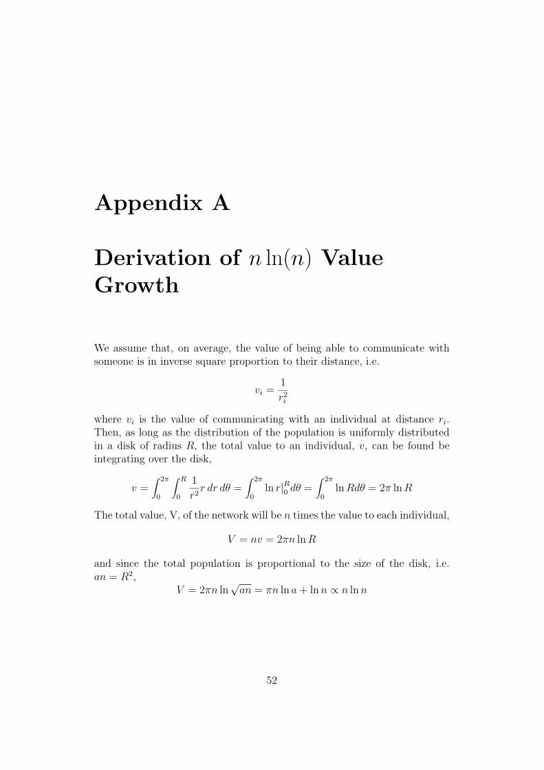
We assume that, on average, the value of being able to communicate withsomeone is in inverse square proportion to their distance, i.e.

vi =1

r2i

where vi is the value of communicating with an individual at distance ri.Then, as long as the distribution of the population is uniformly distributedin a disk of radius R, the total value to an individual, v, can be found beintegrating over the disk,

v =∫ 2π

0

∫ R

0

1

r2r dr dθ =

∫ 2π

0ln r|R0 dθ =

∫ 2π

0lnRdθ = 2π lnR

The total value, V, of the network will be n times the value to each individual,

V = nv = 2πn lnR

and since the total population is proportional to the size of the disk, i.e.an = R2,

V = 2πn ln√an = πn ln a+ lnn ∝ n lnn

52

Appendix B

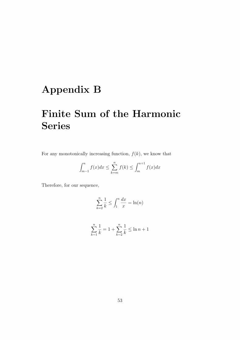
Finite Sum of the HarmonicSeries

For any monotonically increasing function, f(k), we know that

∫ n

m−1f(x)dx ≤

n∑k=m

f(k) ≤∫ n+1

mf(x)dx

Therefore, for our sequence,

n∑k=2

1

k≤∫ n

1

dx

x= ln(n)

n∑k=1

1

k= 1 +

n∑k=2

1

k≤ lnn+ 1

53

Appendix C

Matlab Code

54