Federal Reserve Bank of MinneapolisResearch Department Staff Report 279

September 2000

Growth Cycles and Market Crashes

Michele Boldrin*

Federal Reserve Bank of Minneapolisand University of Minnesota

David K. Levine*

University of California, Los Angeles

ABSTRACT

Market booms are often followed by dramatic falls. To explain this requires an asymmetry in theunderlying shocks. A straightforward model of technological progress generates asymmetries that arealso the source of growth cycles. Assuming a representative consumer, we show that the stock marketgenerally rises, punctuated by occasional dramatic falls. With high risk aversion, bad news causesdramatic increases in prices. Bad news does not correspond to a contraction of existing productionpossibilities, but to a slowdown in their rate of expansion. This economy provides a model ofendogenous growth cycles in which recoveries and recessions are dictated by the adoption ofinnovations.

*We are grateful to Fundacion Marc Rich, DGICYT PB97-0091, NSF grant SBR-9617899 and the UCLA AcademicSenate for support. The paper benefited greatly from comments by two anonymous referees and from conversationswith Boyan Jovanovic, Jose Wynne and Bill Zame. Jose Wynne carried out the simulations. The views expressedherein are those of the authors and not necessarily those of the Federal Reserve Bank of Minneapolis or the FederalReserve System.

1. Introduction

Whenever there is a dramatic fall in the stock market, public discussion centers on

the idea that investor psychology or irrationality is the root cause. Closely associated with

this view is the idea that stock market crashes (and the booms that precede them) are a

bad thing. Even within professional circles, the fact that the stock market rises relatively

smoothly, but falls abruptly is used as evidence for this point of view. Indeed, to explain

the asymmetry in rises and falls, a fundamentalist view of the stock market requires an

asymmetry either in the underlying technology shocks that drive fundamentals or in the

information-processing mechanisms that characterize the market. The first source of

asymmetry has been recently studied by Zeira [18]; the second source of asymmetry has

been studied, for example, in a recent paper by Lee [13]. In this paper we consider the

first case, that is, an asymmetry in the underlying process of technological improvement.

On the face of it, such an asymmetry seems implausible. Our goal is to argue, on

the contrary, that a very natural model of technological progress under uncertainty leads

to exactly the type of asymmetry required to explain gradual rises in the value of the

capital stock, punctuated by sharp declines, provided that traders are not terribly risk

averse. Indeed our contention is that this same model can explain both asymmetric

growth cycles with long recoveries and short and sharp recessions, and asymmetric

movements of stock market prices. This is accomplished without the need for the

unpalatable assumption of technological regress. The evidence presented in Crafts [5],

David [6], Hornstein and Krusell [11], among others, suggests that large recessions may

be triggered by technological innovations and the adoption of new machinery.

Greenwood and Jovanovic [8] and [9] make a related point. They argue that when

a technology plays out, the stock market declines. This may occur because incumbent

firms resist the introduction of the new technology, or it may be because of the need to

train labor as in Greenwood and Yorukoglu [10]. After a period of time, the new

technology is successfully introduced and the stock market rebounds. They focus on the

IT revolution as a case study of the replacement of one technology (main frame

computers) by another (PCs). Unlike in our argument, however, the market does not

recover gradually, but rather suddenly, as the new technology comes on line all at once.

2

The idea that a switch-over between the old and new technology leads to an economic

slowdown can be found in many other places; Atkeson and Kehoe [2] is one example.

Another is Zeira [18], which is closely connected in spirit and basic intuition to this

paper. Like us, Zeira stresses the role played by the arrival of information on stock market

movements and the intrinsic asymmetry between the “good news,” corresponding to a

continuation of the growth process, and the “bad news,” corresponding to a sudden halt of

the growth process. Zeira, however, concentrates on the learning process induced by the

arrival of new information, while we focus on the endogenous growth and technological

innovation side of the problem.

We should also note that we study a one input (capital) model of production, as

for example, in Lucas [14] or Mehra and Prescott [16]. As a result, our model does not

address the controversial issue of correlations between labor inputs and technology

shocks, discussed, for example, in Gali [7].

Our basic model is that of an economy growing due to improving technology

introduced in Boldrin and Levine [4]. In this model, activity analysis is used to model the

existing state of knowledge as a set of currently available activities. This set of available

activities grows over time due to technological progress. In general, to make use of new

activities, it is necessary to introduce new kinds of capital. In this setting, it is natural to

distinguish between research and development—the process of introducing new

technologies and the process of improving old ones. We model this by assuming that

there are many types of capital, each one corresponding to a different underlying

technology. In addition, each technology (type of capital) is available in many

generations. The most rapid form of technological improvement is to upgrade existing

capital to a newer generation. Treating research as “extensive” and development as

“intensive,” Jovanovic and Rob [12] have derived exactly this result in a fairly general

micro-model of endogenous technological process. This distinction is also consistent with

evidence from the applied industrial organization literature. This literature suggests that

new technologies require a long time to be adopted on a large scale and go through

prolonged periods of productivity enhancement before improvement opportunities die

out. See, for example, Mansfield [15].

3

In our model each type of capital (technology) is limited in how many generations

of improvement can be sustained: no matter how much effort we put into it, an improved

bicycle never turns into an automobile. Nevertheless the stage of improvement at which a

capital stock is played out and can be improved no further is not known in advance. When

a technology is played out, however, it is possible to introduce a new type of capital, but

there is necessarily a time delay before the new capital can compete on equal terms with

the old type of capital.

We study an activity analysis economy with constant returns to scale and zero

profits. At each moment of time, capital is a fixed factor and is priced according to the

expected discounted value of future rents, which are in the form of consumption produced

directly or indirectly from that capital. In equilibrium, this price, computed from marginal

rates of transformation, is equal to the price computed from marginal rates of substitution,

such as those used in Lucas [14].

In this economy the basic technology shock is the discovery that an existing type

of capital is played out. What impact does this have on the value of the existing capital

stock? The playing out of an existing type of capital does not reduce the currently

available activities or capital in any way, but it does make future production possibilities

less attractive than they would have been if the technology had not played out. The

impact this has on the market value of the capital stock depends (in our case of CES

preferences) on the coefficient of relative risk aversion. If the coefficient of relative risk

aversion is positive, then the value of capital increases; if it is negative, it decreases. This

is due to the combined impact of the bad news on future interest rates and on future

consumption flows. In the highly risk averse case, interest rates drop sufficiently that

even though the value of future consumption to which current capital is a claim goes

down, the present value actually goes up. This, maybe surprising, feature of asset prices is

not special to our model. It applies to all consumption-based asset pricing models which

adopt a time-separable, CES utility function to value uncertain consumption streams. For

example, in simulations with the Mehra-Prescott [16] model, we find that with the

coefficient of relative risk aversion greater than one, feeding observed consumption

shocks into the model results in stock price movements of an empirically relevant

magnitude, but the wrong sign. This underlying mechanism also means that when

4

consumption growth shocks are positively correlated, the risky asset is a good hedge

against risk, so that with high risk aversion the risk premium is actually negative. This

was first pointed out in Boldrin, Christiano and Fisher [3].

Given our specification for preferences, the case of low risk aversion is therefore

the empirically interesting one, because it corresponds to the stock market dropping on

bad news. We explore in some detail the time path of capital, consumption and prices in

the case in which technology shocks are relatively infrequent. Ordinarily there is no bad

news, and the value of capital gradually increases over time due to the overall growth in

consumption. This is the period of stock market booms. However, following a bad shock,

the value of capital falls abruptly. At this time, a new type of capital is introduced and

used to produce additional generations of the new type of capital, until eventually they are

sufficiently productive to be used in the production of consumption. At this time, the old

type of capital is retired, and the economy resumes its previous growth.

Of particular interest is the transition. Although this period corresponds to one of

technological innovation in the sense that a new kind of capital is being produced for the

first time, it is also a recession. In particular during the transition following the negative

shock, consumption and GNP may rise or decline, but they rise less rapidly than in good

times. During the recession, net investment stalls and a replacement process from old to

new machines takes place. The stock of capital grows at the same slow rate that

consumption does. During this recession, the stock market gradually recovers from its

initial fall.

We also examine the quantitative implications of the theory, showing that in a

realistic range of parameter values, it is possible to generate falls in the stock market on

the order of 10-20%, together with plausible business cycles.

Key to this point of view is the idea that neither the stock market boom, the stock

market crash, nor the recession that follows the crash are bad. Here they are part of a first

best solution to the problem of maximizing the present value of utility from consumption.

Of course, the negative shock is a bad thing in the sense that it would be better if it were

possible for technology to continue improving. However, there is nothing in the working

of the stock market or in the behavior of consumption after the crash that could be

improved upon.

5

At the heart of our results is the underlying idea that technology shocks are

properly thought of as asymmetric. Take, for example, “Moore’s Law,” the “law” that

says that the speed of microprocessors doubles every 18 months. From basic physical

principles, we are confident that this improvement will not continue forever. However, it

is difficult to predict with certainty when it will come to a stop. The discovery that

Moore’s law no longer holds, when it happens, may occur quite abruptly. Consider, on

the other hand, the discovery of a new technology, however, abrupt: there is necessarily a

delay while the new capital is built, the new technology deployed, and the practical

experience (development) needed to use it effectively takes place. It is this basic

asymmetry that we capture here. This asymmetry is especially important when we

consider technological change in a broader perspective. For, at the aggregate level,

technology is not merely the knowledge of how to build things. It is also the institutions

and arrangements for trade, and capital includes the knowledge of how best to make use

of those institutions. So, for example, in a developing country, changes in legal

arrangements such as trade policy or improvements in financial markets can be viewed as

the introduction of a new technology. However, it takes some time for producers and

traders to learn how best to make use of these new institutions. In our model this

corresponds to upgrading the current type of capital. However, the benefits, for example,

of trade liberalization, are not unlimited; in our model, it is the discovery that benefits of

liberalization have been exhausted that triggers a recession and a fall in the stock market.

The rest of the paper is organized as follows. The next section looks at the

behavior of the S&P 500 index over the twentieth century and concludes that the

empirical evidence rejects the hypothesis that stock market movements are driven by a

symmetric Markov process. Section 3 introduces our formal model and shows its

equilibria are efficient. Section 4 characterizes the dynamic properties of such equilibria,

showing, in particular, the differential impact on the value of the capital stock of bad and

good news. We present both qualitative and quantitative evidence of this fact by

simulating the growth cycles generated by the model. Section 5 concludes.

6

2. Is There An Asymmetry Between Rises and Falls?

The first issue is whether there is evidence of the conventional wisdom of

asymmetry in rises and falls of the stock market. The purpose of the simple data analysis

we are going to present next is not to test our model, although detailed testing would be

valuable in future work, but rather to show that asymmetry is potentially a real puzzle that

needs to be explained. We should point out that our explanation of asymmetric shocks or

responses to shocks is not the only one—see, for example, Zeira [18] and Lee [13] for

interesting models of how informational dynamics can lead to stock market overshooting

and corresponding asymmetries.

In the Appendix, we reproduce from Shiller [17] the real Standard and Poor’s

Index annually from 1889-1984. We also calculate the logarithmic differences from one

year to the next as a deviation from the mean. The mean logarithmic growth rate during

the period was 1.0%.

The “common wisdom” we wish to verify is that increases are smaller and more

persistent than decreases. In the table below we compute the length of runs of deviations

above (+) and below (-) the mean growth.

This provides some preliminary evidence of asymmetry: runs of positive

deviations are longer than those with negative deviations, and there are more positive

than negative deviations. The fact that there are more positive than negative deviations is

also reflected in the fact that positive deviations are on average smaller than negative

Run + -

5 2 0

4 2 1

3 2 1

2 9 11

1 9 12

51 41

7

deviations: the average positive deviation is 12.3%, while the average negative deviation

is -16.0%. This difference of 3.7% is reasonably large in economic terms.

If shocks to growth are symmetric around the mean and i.i.d., how likely is it that

these differences are due to sampling error? A simple test is to fit a two state Markov

model in which the probability of the next sign depends on the previous sign. The

maximum likelihood estimates are derived by computing the frequency of + separately,

conditional on the previous sign. If the previous sign was +, the probability of another +

is 53%; if the previous sign was -, the probability of a + is 61%. We can also compute

standard errors for each of these coefficients, subtract 50% and normalize: conditional on

+ the normalized value is 41%; conditional on - the normalized value is 141%. The

probability that the first value is 41% or more (using the normal approximation to the

binomial) is 34%; the probability that the second value is 141% or more is 8%. Since the

two values are independent of one another under the i.i.d. assumption, the probability that

both events occur is just the product of the two probabilities: 2.7%. So if the data are truly

symmetric and i.i.d. there is only a 2.7% chance of the observed discrepancy.

3. The Model

3.1. The State Space

We use a standard infinite horizon event tree model of time and uncertainty. Dates

are denoted by t � 0 1 2, , ,� . At each date t there are possible a countable number of states

� t I� . A state history s t� ( , , , )� � �0 1 � is a finite history of states. The (countable) set

of all state histories is denoted by S. For a given state history s t� ( , , , )� � �0 1 � , we let

t s t( ) � denote the terminal time and η t the terminal state. We also order state histories

so that ~s s� if t s t s(~) ( )� and ~� �t t� for � � t s( ) . We write s�1 for the immediate

predecessor of s and s+ for the set of immediate followers of s. We let � s denote the

probability of state history s, so that π ss t s t�

=

� 1: ( )

.

3.2. Households

There is a single representative household, who following the state history s

consumes cs ��+

. This household receives total lifetime utility of � �t sss S su c( ) ( )

³� ,

where 0 1≤ <δ is a subjective discount factor. Rather more strongly, we will assume that

8

the period utility function is smooth, concave, bounded below, and, at least for levels of

consumption above a subsistence level c c� , has the CES (or constant relative risk

aversion) form u c c( ) ( / )� � -1 � q , where θ � �1 0 is the coefficient of relative risk

aversion. Note that for � � 0 the CES function is not bounded below, which is why we

require this functional form only for levels of consumption above subsistence. As we are

interested in the theory of growth, not the theory of subsistence, the behavior of u for

small quantities of consumption is not terribly interesting. In particular, in the equilibria

we consider, consumption will be uniformly bounded away from zero, and we will

assume that this bound exceeds the subsistence level. This means that we can assume that

utility is bounded below, which is technically useful, while nevertheless having the

convenience of the CES functional form.

3.3. Production Possibilities

There are a countable number of types of capital � � 0 1, ,� . Each type of capital

is potentially available in a countable number of generations i � �� �, , , ,1 0 1 . We denote

by k iω the amount of type � capital of generation i . We refer to a type/generation pair as

a kind of capital. Production takes place through linear activities, using capital as input.

We begin by describing all potential activities, although not all of these activities are

available at any moment of time, and indeed, some activities may never be available.

Each activity takes as input one unit of capital of a specific kind and produces a

single output in the following period. Type � capital of generation i may be used as the

input into 4 distinct activities, each of which is characterized by the output obtained:

1) γ i units of the consumption characteristic, � 1

2) � 1 units of the same kind of capital: type � capital of generation i

3) ρ β ρ: 1 units of the next generation of capital: type � capital of generation i +1

4) 1 unit of type � �1 capital of generation i L− , L 0 .

We assume that � � , so that more consumption can be obtained by moving to the next

generation of capital than by remaining with the current generation. Notice that we do not

presume that the increased consumption from higher generations of capital takes place

9

through the physical production of increased units of some commodity. The increased

amount of characteristic may take place through the production of more advanced

commodities which contain more of the characteristic that is actually consumed.

However, to keep notation to a minimum, we will not explicitly introduce the distinction

between the amount of commodities produced and purchased and the amount of

characteristic consumed.

At each moment of time, only a finite number of this countable collection of

activities are actually available. The set of available activities is determined by the state,

which we take to be a list of those activities that are available. We now describe both the

set of possible states and the state transition process that determines � s , the probabilities

of state histories.

A state � �I consists of a latest type of capital � �( ) , and for each type of capital

� � �� ( ) a latest generation of capital i ( , )ω η , plus a number 0 � m( )� (this number is

used to track the time since the latest type of capital was introduced). The available

activities are these: if ω ω η ω η≤ ≤( ), ( , )i i then all four activities making use of k iω are

available, with the following exceptions:

1) if ω ω η ω η< =( ), ( , )i i then activity 3 producing the next generation of capital is not

available

2) if ω ω η ω η= ≤( ), ( , )i i then activity 4 producing the next type of capital is not

available.

On the other hand, if � � � ( ) or i i> ( , )ω η then no activities making use of k iω are

possible.

The interpretation of the state is this: except for the latest type of capital,

improvements on other types of capital have stalled, and it is no longer possible to

produce new generations. New types of capital can be introduced, from the very latest

type of capital and its latest generation, only when the opportunity for producing new

generations of the latest type of capital has vanished. The latter assumption deserves

some comment. It amounts to saying that experimentation with future technologies

cannot take place while the current technology is being used and improved. If this were

10

not the case, a benevolent planner could take advantage of the constant returns to scale

nature of our activities and run the technology ω +1 at an infinitesimal scale to acquire

valuable information about the generation at which it will play out. This information is

valuable because it eliminates the uncertainty about future consumption growth rates. As

a result, it also modifies the current market evaluation of the existing stock of capital and

makes stock market prices a monotone deterministic process. This assumption is

therefore needed to retain a minimum of uncertainty about future technological evolution.

The states follow a Markov process. Fix an initial state � . We define the next

generation of capital as the state ηg in which ω η ω η( ) ( )g = , i ig( , ) ( , )ω η ω η= for

� � � ( ) , i ig( ( ), ) ( ( ), )ω η η ω η η= +1, and m mg( ) ( )η η= +1 . We define the next type of

capital as the state ηb in which ω η ω η( ) ( )b = +1 , i ib( , ) ( , )ω η ω η= for � � � ( ) ,

i ib( ( ), ) ( ( ), )ω η η ω η η= +1, i i Lb b( ( ), ) ( ( ), )ω η η ω η η= − −1, and m b( )η = 0 . Starting at

� , only η ηg b, can be reached with positive probability. If m M( )� � then, with

probability 1, ηg is reached. On the other hand, if m M( )� with probability 1�� the

state moves to ηg and with probability � the state moves to ηb . This means that for M

periods following a transition from state � to state ηb there is no uncertainty about the

ability to build new generations of the new type of capital. Since we view � as relatively

small, this assumption does have much economic import. However, by carefully choosing

M we can greatly simplify computations as we indicate below.

We will frequently refer to that transition from � to ηb as a negative or bad

shock to technology. Similarly, we will call ηb , which is characterized by m b( )η = 0 ,

the negative or bad state. But notice that the technological possibilities at ηb are a strict

superset of those available at � . All activities that were available at � are still available

at ηb . In particular, we do not assume that a negative shock simply causes the current

capital stock to retrogress or become less productive. Indeed, we may wonder why it

would ever be desirable to switch to a new kind of capital, which is, after all, essentially

identical to the current kind of capital. The answer is that despite the fact that the new

kind of capital is actually inferior to the old kind of capital, development of new

generations of the old kind of capital is impossible. Switching to the new kind of capital

makes it at least possible to introduce higher generations of capital.

11

3.4. Production Plans

At any moment of time there are in principle a countable number of different

types of capital. Let k Xs � be the vector of different kinds of capital when the state

history is s. The components of ks are ksiω . An activity may be thought of as a triple

( , , )x y c , where x y X, � are the capital inputs in period t and output in period t �1, and

c ��+

is the amount of characteristic output in period t �1. Let A be the set of all

potential activities, and recall that � are those actually available when the state is � . An

activity vector s is a map s A: ��+. Feasible activities are given by sets A As ⊆ ,

with A0 ≠ ∅ and for ~s s≥ that A As s~ ⊇ . A production plan consists of a map from state

histories S to capital vectors ks , consumption of characteristics cs (for t s( ) 0 ) and

activity levels λ s sA∈ . We say that the production plan is feasible with respect to the

initial condition k0 0,� if for every state history s with � s 0

λ

λ

λ

η

η

η

sa s

sa s

s sa

a y a k

a c a c

k a x a

s

s

s

-³

-³

- -³

-

-

-

��

�

�

�

�

1

1

1 1

1

1

1

( ) ( )

( ) ( )

( ) ( ).

We call an activity viable for the state history s and initial condition k0 if there exists a

socially feasible production plan such that s a( ) 0. We denote the set of viable

activities for state history s by A ks ( , )0 0� . We assume that the initial set of activities

A k0 0 0( , )η is non-empty for k0 0≠ and that for ~s s≥ , A k A ks s~ ( , ) ( , )0 0 0 0η η⊇ . Note that

A ks ( , )0 0� may be a proper subset of the set of feasible activities in � s . Similarly, we call

a kind of capital viable for the state history s and initial condition k0 0,� if there exists a

socially feasible production plan such that there is a positive amount of it available at s.

Finally, we say that a production plan solves the social planner problem for initial

conditions k0 0,� if they solve max ( ( ) ( ))( )δ λ πηt s

sas S su a c as

−∈∈ ∑∑ 1 subject to social

feasibility.

3.5. Prices

Let qs be the present value price of different kinds of capital when the state

history is s, and let ps be the corresponding present value price of the characteristic. In a

competitive equilibrium, these prices should satisfy two conditions: they should yield

12

zero profits and support the preferences. Specifically, we say that prices yield non-

negative profits for the initial condition k0 0,� if

p c a q y a q x a a A k sss sσ σσ η( ) ( ) ( ) , ( , ),� � � � � �³

+� 0 0 0 ,

and if this holds with equality, we say that the activity a yields zero-profits. We say that

the prices support the consumption plan �cs if �cs is a solution to

arg max ( )( )δ πt sss S su c∈∑ subject to

p c p cs ss S s ss S³ ³� �� � .

The first order conditions for the consumer are satisfied if

� 0 p u cst s

s s� �µδ π( ) ( ) with equality unless cs � 0 .

Here µ is the marginal utility of consumption. Note that this first order condition is valid

for all values of cs > 0, but that for c cs < the period utility function u does not have the

CES form, as we discussed above. The first order condition is most useful in the case of

an interior solution where c cs s-

1 0, , in which case

δ ππ

s

s

s

s

s

s

u c

u c

p

p- - -

��

�1 1 1

( )

( ).

Finally, we say that prices and capital ks satisfy the transversality condition if

lim| ( )T s ss t s T

q k→∞ =∑ = 0 .

3.6. Efficiency

We show how to characterize the solution to the planner’s problem by a relatively

standard price decentralization scheme, despite the fact that there are infinitely many

kinds of capital, and those actually available grow over time.

Proposition 3.1: Suppose that � , � , � s s sk c are socially feasible for the initial condition

k0 0,� and that δ πt ss ss S

u c( ) ( � ) < ∞∈∑ . Then the following three conditions are equivalent

(1) � , � , � s s sk c solve the social planner problem for initial condition k0 0,�

13

(2) there exist prices �, �q p that satisfy the non-negative profit condition, yielding zero

profits for all activities for which � ( )λ s a 0 and support the consumption plan �cs with

� �p cs ss S³� �

(3) there exist prices �, �q p that satisfy the non-negative profit condition, yielding zero

profits for all activities for which � ( )λ s a 0 , the first order conditions and the

transversality condition.

Proof: First we observe that if the profit conditions hold, then the transversality condition

is equivalent to the consumption plan having finite value. Indeed, from the zero profit

condition

q k q k q k q k p css t s T s s s s ss t s tt

T

s ss t s tt

T

0 0 1 1 110 10� � � � �

| ( ) | ( ) | ( )− = − == + − −= += = +=∑ ∑∑ ∑∑ .

Next we consider the T-truncated utility economy with utility function

δ πt sss t s T s s ss t s T

u c q k( )| ( ) | ( )

( )≤ = +∑ ∑+1

.

We observe that when we eliminate states with zero probability and non-viable kinds of

capital, this is an ordinary finite economy. By standard methods, a production plan� , � , � s s sk c solves the social planner problem if and only if its truncations solve this

truncated problem. The equivalence of (2) and (3) to zero now follow immediately from

the corresponding facts for the finite horizon case.

�

4. Analysis of the Model

Let us begin by defining the most advanced kind of capital in state � to be capital

of type � �( ) and generation i ( ( ), )ω η η if m( )� � 0 , and capital of type � �( ) �1 and

generation i ( ( ) , )ω η η−1 if m( )� � 0. Fix the initial condition �0 . We will now analyze

the model under three assumptions: first, that the parameters � � �, , satisfy the hypothesis

of Proposition 3.1 so that an optimum exists; second, that M is relatively large compared

to L; and third, that the initial stock of capital consists solely of the most advanced kind

of capital in state � 0 .

14

4.1. Basic Results

It will be helpful to begin with a very simple problem: suppose that capital of a

particular type is stalled. More specifically, suppose that there is a single unit of

generation 0 capital of this particular type, so that we are contemplating producing some

output of the characteristic t �1 periods from now on using one of two methods. First,

we can simply build more of the existing type and generation of capital until period t �1,

yielding � t-1 units of characteristic. Second, we can build a unit of the next type of

capital of generation �L , then use that to build generation � �L 1 and so forth until

period t �1. This yields ρ γt t L- - -2 2 units of characteristic. If we define

mL

*( ) log log

log log log� � � �

� �1

1 γ ρρ γ β

and make the generic assumption that this is not an integer, then for t m� * we would

prefer to use the old kind of capital, while for t m� * we would like to use the new kind

of capital.

Proposition 4.1: If M m� �* 1 and the initial stock of capital consists solely of the most

advanced kind of capital in state �0 , then with probability 1 in every subsequent state �

there will be a positive amount of the most advanced kind of capital available. Moreover,

there will be a positive amount of at most one other kind of capital, and this will be of the

type immediately preceding the most advanced kind. Moreover, the negative state

m( )� � 0 can occur only when there is a single type of capital.

Remark: As we shall see below, the equilibrium switches between using a single type of

capital to produce consumption and new capital. Then, when that kind of capital is played

out, the older kind of capital is used to produce the consumption good and reproduce

itself, while the new kind of capital is used solely to produce new generations of itself.

Finally, when sufficiently advanced new generations of the new kind of capital are

produced, the old kind of capital is abandoned completely, and the cycle begins anew. Of

particular interest is the transition when two kinds of capital are in use. We explicitly

solve for prices, output and so forth below. However, we should give the intuitive idea of

what happens during the transition.

15

During the transition, the new kind of capital is relatively unproductive at

producing current consumption. However, it is quite productive at producing (indirectly)

consumption a number of periods into the future. At equilibrium prices, firms are

indifferent between using activities involving either producing consumption from the old

kind of capital or activities producing new generations of the new kind of capital. The

price at which those new generations can be sold reflects the fact that ultimately they will

be used to produce consumption goods. If we think of the new generation of capital as

being retained within the firm rather than sold in the market, the firm producing the new

generations of capital will have negative cash flow. Since the new kind of capital is not

being used to produce consumption, the activity of producing new generations can be

viewed as development—learning to produce more advanced generations of capital. The

output from this D part of R&D is more advanced capital, which is either sold or retained

within the firm. The activities of Internet startup firms, which have high capitalized value,

yet have negative cash flow, can be interpreted as engaging in this development activity:

IPOs correspond to selling the relatively advanced generation of capital that has been

produced over a number of years within the firm.

Proof: In the good state if there is one kind of capital, then, since �� �� , the next

generation should be the only kind produced. On the other hand if the bad state occurs at

time � , then there is no uncertainty about the technology available through period

� � M . Observe that if we produce consumption for period � � t by producing the old

kind of capital until period � � �� � � � �T t 1 then output of consumption at � � t is

proportional to β ρ γT t T t T L- - - - -2 2 , which, since �� �� , is strictly decreasing in T . This

implies that it is always best to produce the new capital right away. Now consider t the

least integer greater than m* . Since M m� �* 1 there is no uncertainty about the

availability of generation t L� of the new type of technology to produce consumption

for period t and all subsequent periods. It follows that no capital of the old kind should be

produced beginning in period t �1 (or of course any later period). Also since M t� �1 ,

it is impossible to produce any capital of a higher kind than the newest kind in period

t �1 . Consequently in period t �1 the only type of capital is the most advanced kind in

that state, giving the desired result.

�

16

Suppose now that only the most advanced kind of capital is available, and denote

the most advanced kind of capital in state � by z( )� . Let V ks sz s( , )( )� h be the lifetime

value of future consumption beginning in this state with ksz s( )h units of the most advanced

capital. Notice that having k i units of generation i capital will simply result in γ i ik times

as much consumption in every future time and state as with a single unit of generation 0

capital. If we take Vm to be the value of a single unit of generation 0 capital (of any type)

when m m( )� � , we can write

k k Vs sz i

sz

ms s s s

s( , )( ) ( ( ), ) ( )

( )η γη ω η η η

θ

η=−� � ,

for m � 0 and for m � 0

k k Vs sz i

szs s s s( , )( ) ( ( ) , ) ( )η γη ω η η η

θ= −

−1

0� � .

Notice also for m M� that V Vm M� .

Notice that capital is produced for period t before the state at period t is known,

but is used in period t after the state is determined. Consequently, we can compare the

value of the capital stock (relative to the price of consumption) at time t immediately

before and immediately after the state is realized. Our goal is to show that good news has

a marginal impact on the value of capital, but bad news causes it to change abruptly.

Proposition 4.2: Suppose M m� �* 1 and the initial stock of capital consists solely of the

most advanced kind of capital in state �0 . When − ≤ <1 0θ , news of a negative shock

m( )� � 0 causes the value of the capital stock to fall immediately. If � � 0 the value of

the capital stock rises immediately. Precisely, the ratio of the value of the capital stock

after the announcement to that before is given by

� �( )1 0V

VM

.

Remark: The same method of proof shows that good news causes the stock market to

change by

17

( )10

� � V

VM .

From an economic perspective, the interesting case is when time intervals are relatively

short, so that is small. Notice, however, that it is not the case that shorter time intervals

lead V VM0 1/ � : the need to switch to a new technology has an appreciable utility cost

regardless of how time is measured. This means that for short time intervals, to a good

approximation, good news has little effect on the value of the capital stock, while bad

news causes it to change by V VM0 / .

Proof: Since the capital stock and current consumption are both fixed, the only question

is what happens to the price of the capital stock. If in the current period m( )� � 0 it must

be that in the previous period m M( )� � . In addition, by Proposition 4.1 in the current

period there is a single type of capital of the most advanced type. Suppose that the

amount of this capital is ksz( )η . If there is not a negative shock in the current period then

the value will be

γ ω η η ηθ

isz

Mg g k V( ( ), ) ( )� �

−;

if there is a negative shock the value will be

γ ω η η ηθ

iszb b k V( ( ) , ) ( )−

−1

0� � .

The corresponding prices at which capital ksz( )η is traded are determined by differen-

tiating these values with respect to ksz( )η . Notice that i ig g b b( ( ), ) ( ( ) , )ω η η ω η η= −1 ,

since the ability of the capital to produce next period consumption is not changed by the

shock. Consequently the price of capital without the negative shock is proportional to

��VM , and with the negative shock to ��V0 . Clearly V VM0 � . If � � 0 this means that

� � �� �V VM 0 , while if � � 0 this means that � � �� �V VM 0 , which is the desired result.

�

Proposition 4.2 shows that when time intervals are short, good news has a

marginal impact on stock prices, while bad news causes them to change abruptly. We

reinforce this by showing that once the good state is sufficiently well established,

18

meaning m M( )� � , the value of the capital stock from period to period rises

exponentially and, in the continuous time limit, continuously.

Proposition 4.3: Suppose M m� �* 1 and the initial stock of capital consists solely of the

most advanced kind of capital in state �0 . When m Ms( )� �

q k p

q k p

V

Vsz

sz

s

sz

sz

s M

s s

s s

( ) ( )

( ) ( )

/

/( ) ( )

h h

h h

q

q

q

q

�� � - - -

+

-

+

+

- -

� � ����

���1 1 1

1

1 1 0

1

1

1 11 .

Proof: Observe that since m Ms( )� � , the economy is following balanced growth, and in

particular the relative price of capital to consumption is not changing. So the growth in

the value of capital is due entirely to the increased size of the capital stock:

q k p

q k p

k

ksz

sz

s

sz

sz

s

sz

sz

s s

s s

s

s

( ) ( )

( ) ( )

( )

( )

/

/

h h

h h

h

h

- - - -

- - -

�1 1 1 1

1 1 1.

Without loss of generality, take ksz s-

- �11 1( )h ,i s s( ( ), )ω η η− − =1 1 0. Then the Bellman

equation is

V u V VM M� � � � �-� �� f

qmax ( ) ( ) ( )1 1 0 .

The first order condition for the optimum is

� �� q q q- - -

- -� � � ����

��� �1 1 01 1 0( ) ( )� � V

VV

MM ,

while from the Bellman equation

VV

VVM

MM� � � � � �

���

���

-

-��� � �� � � �q q1

1 1 0( ) ( )� �

or

VVV

M

M

� �� � � �

���

���

-

-

���

� �� � � �

q

q

1

1 1 1 0( ) ( )� �.

Substituting back into the first order condition, we find

19

� � �� � � �q

q

q

q

1 11

1 1 0

1

1

� � � ����

���

+

-

+

+� � ( ) ( )V

VM

,

which is the desired result.

�

4.2. Dynamic Analysis

We now examine in greater detail the time path of consumption and capital

following a negative shock. Without loss of generality we may begin at time 0 in state

�0 , assuming that a negative shock has just occurred. We may also assume that there is

only one kind capital, that this is type 0 generation 0, and that there is 1 unit of this

capital, as well as c0 units of characteristic produced from last period. We also assume

that current capital is the most advanced possible given the technology, so the initial state

has � �( )0 1� , i( , )0 00η = , i L( , )1 10η = − − and m( )�0 0� .

In this analysis it is convenient to take M to be the largest integer smaller than

m* . This means that as soon as the economy switches from two kinds of capital to one, it

is possible to have negative shocks once again. This simplifies computations without

detracting a great deal from the economics.

Suppose that 0 � �t M . Notice that during this period, only the old kind of

capital is used to produce consumption, and so from the zero profit condition the market

discount factor from period t to period t �1 is p pt t+

-�11/ . In the interior the

household must be on the margin between consuming in periods t and t �1, so by the

first order condition

� q

c

ct

t+

+

-������ �

1

1

1.

From this we can derive the growth rate of consumption from periods 1 to M.

c

ct

t

++�11

1� q� � .

During this period the new type of capital will grow at the rate � , as it is not used to

produce consumption. We summarize this information in the table below.

20

t ct kt00 kt

t L1 1( )- -

0 c0 1 0

1 c1 k100 k L

11( )-

2 � q� � 1

11

+ c k200 �k L

11( )-

� � � �

M �� q M

c-

+

1

11 k M

00 ρ M M Lk− − −111 1( )

M �1 �� q M

c+11 0 ρ M M Lk1

1( )−

We can also work out the amount of old capital required for 0 � �t M :

k c kt t t00

11

100� �

+

-

+� .

From this we can find

k c MM

M

100

11 1

0

1� - - -

-

+

=

- � ��t

t

q

t

( ) .

We also require that period 1 output be produced from period 0 capital

(1) k cL MM

M

11

11

11

1

1

1 11

1

( )- -

+

-

+

-

+

� � �� ���

���

� ���

���

�

�

����

�

�

����

�

�

����

�

�

����� ��

� ��

� ��q

q

q

.

Finally, observe that initial capital can be used either to produce period 1 consumption,

yielding a marginal lifetime utility of δ u c( )1 , or to produce period M �1 type 1 capital

of generation M L� . This yields an equal marginal lifetime utility of

δγ ρ

δθ

MM L M L

M

L

d k V

dku c+

- --

-� 1 1

1

11 1

( )

( ) ( )� �

21

or

(2) � �-

-

-

- -

- -� � � �q q

qM M L M LMk V c � �1

1 1

11( ) .

Next we must calculate lifetime utility beginning in the negative state:

(3) V c k V

M

M M L M LM0

11

1

1

1

111

1

1= −

− ���

���

−+− −

−+

+

−+

+ − − −θ δ

δ βδ

δ βδδ γ ρθ

θθ

θθ

θ( ) ( )

� .

Notice also that in the good state, the fraction of the capital stock devoted to consumption

� must be constant. Consequently one unit of capital in the good state will produce φγ i

units of the characteristic and ( )1�� � units of the next generation of capital. This leads

to the Bellman equation

V u V VM M� � � � � �- -� � � �� � � � �f

q qmax ( ) ( ) ( ) ( ) .1 1 1 0

The first order condition determining � is

� ��� � �� � ��� � �q q q- -

- - - -� � � � � �1 1 1

01 1 1 0( ) ( ) ( )� � � �V VM

or

(4) �� � �� ���q q q

�� � �-

- +

1

1 1 0

1

1( )� �� �V VM

,

while the Bellman equation for this value of � gives

V V VM M� � � � � � �- - -

-

- -�� � � � � �� � � ��q q q q q101 1 1( ) ( ) ( )� � .

Solving this for V0 we find

(5) VVM

0

11 1 1

1�

� � � �

�

-

-

- -

- -

� � � �� �� �

� � ��

q q q

q q

( ) ( )

( )

� �� �.

The 5 numbered equations must be solved for the unknowns c k V VLM1 1

10, , , ,( )- � . By

directly substituting (1) into (2) and (3), (3) into (4) and (5), and (4) into (5) this may be

reduced to two equations in the unknowns c VM1, .

22

4.3. Quantitative Aspects of the Theory

To get a handle on the implications of the theory, it is useful to consider the

extreme case in which bad shocks are rare, so that � � 0 , and in which new technologies

are difficult to get on line, so that L �� . This will result (for given values of the other

parameters) in the most extreme stock market fall.

Using (4) and (5) above, we may explicitly solve for � and VM when � � 0 :

11

1� � -

+� � �� q q( )� �

VM � �

���

��

-

-

+

+

� �

� �� q q

q

1

1

1

1

1 ( )� �.

Let g denote the growth rate of consumption (in the good state); then g � ��� �( )1 , and

we may substitute in the expression for 1�� to find �� �q� +g 1 / . This gives the value

of the capital stock in terms of the growth rate of consumption and the subjective

discount factor

V

g

M � �

���

��

��

��

-

-

+-

+

� �

�q

q q

q

1

1

1

1

1

.

For the case where L is large, once the technology plays out, the time it takes for a

new kind of capital to come on line is excessively long. So we can regard the bad state as

similar to the good state, but with a potential growth rate of consumption of � rather than

�� . If we let gb denote the essentially fixed growth rate of consumption in this state, we

can find V0 by replacing g with gb in VM . This yields

V

V

g

gM

b

0

1

1

1

1

1

1

1

1

=

−��

��

��

��

−��

��

��

��

−+ −

+

−+ −

+

δ

δ

θθ θ

θ

θθ θ

θ .

Notice that as the logarithmic case is approached, so � � 0 , that V VM0 1/ � as

asserted by Proposition 4.1. Notice, however, that it is also the case that as � � �1 (so

23

the utility function approaches linearity) V VM0 1/ � . So it is the intermediate range

between the logarithm and linear utility functions that is of interest.

Notice that the market rate of interest is � q/ g +1 in the good state, and similarly it

is δ θ/ gb+1 in the bad state. To explore more carefully, let us suppose that gb = 1 so that

there is no growth following a negative shock. In this case the market rate of interest in

the bad state is simply the subjective discount factor. First take this to be 5%, so that

� � 0 95. . If the rate of growth of consumption in the good state is 5%, we may calculate

the variations in the market value of the stock of capital caused by the bad shock for

different levels of risk aversion. This is reported in the next table, along with the interest

rate in the good and bad states.

� -.1 -.2 -.4 -.8

1 0�V VM/ 6.8% 9.9% 9.6% 1.4%

Interest at M 9.1% 8.6% 7.7% 5.9%

Interest at 0 5.0% 5.0% 5.0% 5.0%

Notice that the size of the market drop in the intermediate range of � is not terribly

sensitive to the value of � . In this range the market drops roughly 10% in response to bad

news. If we consider a more drastic fall in the rate of consumption growth from 10% to

0%, we find the following.

� -.1 -.2 -.4 -.8

1 0�V VM/ 13.4% 19.8% 19.7% 2.9%

Interest at M 12.8% 12.0% 10.3% 6.8%

Interest at 0 5.0% 5.0% 5.0% 5.0%

Here, the market drops on the order of 20%.

24

However, in these examples, the market interest rate in the bad state is 5%, which

is high by historical standards. If we reanalyze a change from 5% to 0% growth with

� �.98 , we find the following.

� -.1 -.2 -.4 -.8

1 0�V VM/ 17.8% 26.4% 27.8% 2.9%

Interest at M 6.2% 5.8% 4.8% 4.4%

Interest at 0 2.0% 2.0% 2.0% 3.0%

This means a nearly 30% drop in the market. The reason that greater patience leads to a

more significant market fall is that the bad shock has no consequence for next period

consumption, but the difference in future production possibilities grows over time.

While we cannot pretend that the present, simplified model provides a realistic

account of observed movements in stock market prices, it is still worthwhile to assess the

extent to which the model is roughly consistent with the historical evidence. To this end,

we first consider the quality of our simple approximation and then present the results of a

simulation of the model for parameter values that are not altogether impossible.

We have not tried to calibrate our model to available U.S. data, as our framework

does not incorporate an explicit labor supply rule, nor does it contain other sources of

shocks beyond the “large” and infrequent shocks provoked by major technological

changes. During the majority of periods in which the existing technology is being

improved, there are no other shocks in our model and both quantities and prices follow a

deterministic path. Real economies are affected by many other smaller but more frequent

shocks that lead to large fluctuations in hours worked, quantities produced and market

prices.

Further, we are using a very aggregate model in which only two types of capital

are in use at each moment of time. It is hard to imagine that we can approximate real

market fluctuations terribly well with a model in which there is a single sector of

production and a single technology which is occasionally dismissed to be replaced with a

25

new one. A more realistic model would require several capital sectors, each with its own

technology shocks, and a more elaborate technology for the production of the final

consumption good involving various kinds of capital as well as labor. This would, of

course, require an explicit analysis of the flow of resources between sectors in response to

shocks, as well as an explicit evaluation of the degree of substitutability among inputs in

the various sectors. This is a very interesting task which, nevertheless, goes beyond the

scope of the present, theoretical, paper and is left to a future investigation.

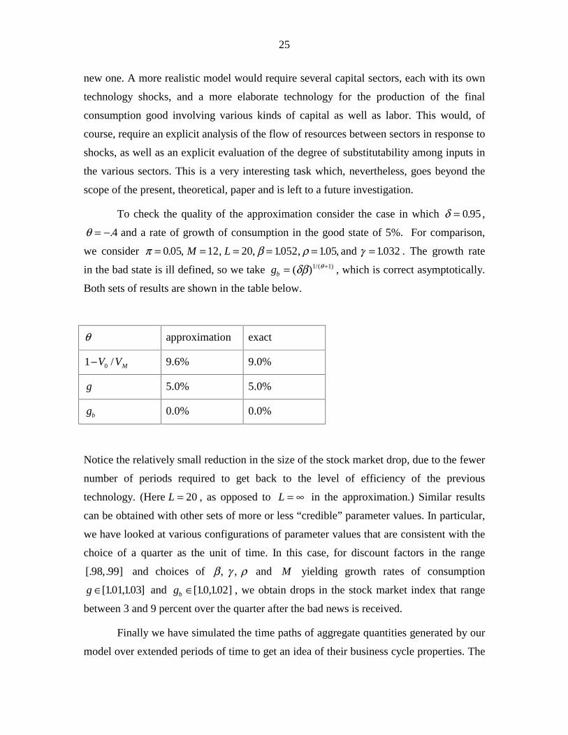
To check the quality of the approximation consider the case in which � � 0 95. ,

θ = −.4 and a rate of growth of consumption in the good state of 5%. For comparison,

we consider π β ρ γ� � � � � �0 05 12 20 1052 105 1032. , , , . , . , .M L and . The growth rate

in the bad state is ill defined, so we take gb = +( ) /( )δβ θ1 1 , which is correct asymptotically.

Both sets of results are shown in the table below.

� approximation exact

1 0�V VM/ 9.6% 9.0%

g 5.0% 5.0%

gb 0.0% 0.0%

Notice the relatively small reduction in the size of the stock market drop, due to the fewer

number of periods required to get back to the level of efficiency of the previous

technology. (Here L = 20 , as opposed to L = ∞ in the approximation.) Similar results

can be obtained with other sets of more or less “credible” parameter values. In particular,

we have looked at various configurations of parameter values that are consistent with the

choice of a quarter as the unit of time. In this case, for discount factors in the range

[. ,. ]98 99 and choices of β γ ρ, , and M yielding growth rates of consumption

g ∈[ . , . ]101103 and gb ∈[ . , . ]10 102 , we obtain drops in the stock market index that range

between 3 and 9 percent over the quarter after the bad news is received.

Finally we have simulated the time paths of aggregate quantities generated by our

model over extended periods of time to get an idea of their business cycle properties. The

26

figure below reports the time paths of the stock of capital and the flow of consumption

generated by a simulation calibrated using the parameters from the last table. Over the

time period considered we observe the introduction and consecutive replacement of three

different types of capital stocks. The overall pattern is clear and qualitatively acceptable.

Accumulation occurs slowly, while dismissal is fast and, in the initial period, abrupt.

Observe that when the bad news arrives the process of accumulation stops for a while.

During this period only replacement of machines takes place: the old type of capital is

used only to produce consumption, while the new kind of machines are accumulated and

the sum of the two stocks remains constant from one period to the next. At the end of the

replacement period the stock of new machines is equal to the stock of old machines when

the recession began, after which net accumulation of capital resumes again. The path of

consumption follows along. As predicted, consumption recessions start at the time at

which the old technology cannot be improved any further and continue after that for a

relatively long number of periods, while the new capital good is improved and

accumulated.

27

One can distinguish the consumption recession periods, in which there is no

growth, and the good periods of high growth beginning when the replacement of the old

technology is completed. The cyclical growth pattern of aggregate output can easily be

inferred from the separate behavior of ct and kt by recalling that, in the practice of

National Income Accounting, output is computed by normalizing relative prices in a base

year. In our case, we can, for example, use the relative price of capital at the beginning of

the recession period to compute net aggregate output as the sum of the consumption flow

plus the net investment flow. The latter is zero during the transition; therefore, output

growth would be also nil during this period. When recovery begins, output of the

investment good becomes positive and consumption growth resumes; hence, aggregate

output growth would increase sharply and converge toward its balanced growth level until

the next recession strikes. If, contrary to National Income Accounting practices, one takes

into account the changes in the relative prices of capital goods, output growth will be

slightly positive even during the recession periods, but still much lower than during the

periods of high growth, and persistent oscillations in growth rates will still appear.

Capital Stockdotted line is consumption

0

1

2

3

4

5

6

1 7 13 19 25 31 37 43 49 55 61 67 73 79 85 91 97 103 109 115 121 127 133 139 145 151 157 163 169

Period

28

Stock market crashes occur at the beginning of recessions and continue for a while

after. Notice that, because of the change in the relative price of capital we just mentioned,

stock market valuations begin to recover before consumption growth does. Hence stock

market values are good predictors of subsequent movements in total output growth.

5. Conclusions

We have constructed a model of long-run growth due to major technological

innovations, improvement of existing machines and substitution away from old

technologies toward new ones when the former cannot be improved any further. Our

theoretical model predicts, in a stylized fashion, that the following sequence of events

should be observed.

When an old mode of production (technology) cannot be improved further, it is

dismissed and progressively replaced by a newer one, which allows for additional periods

of productivity gains and balanced growth. The dismissal of the old technology and the

introduction of new machines trigger recessions. They continue for a few periods while

the new technology is being developed, but end before development of the new machines

is completed. Recoveries settle in slowly and correspond to the phase in which the new

capital good is being adopted and improved to its maximum productivity potential. After

the initial period, recoveries accelerate, leading to a phase of balanced growth that lasts

until the next innovation takes place. Hence, recessions are shorter than recoveries, but

more abrupt. The growth rates of aggregate output persistently oscillate around a kind of

average balanced growth rate. As in other models of growth and innovation, such as that

of Aghion and Howitt [1], recessions are a consequence of the adoption of new

technologies. Contrary to those models, recessions are not due to the fact that labor

invested in R&D does not contribute to aggregate output. They are instead due to the

sudden drop in the ouptut of the investment good and to the reduction in the growth rate

of the consumption sector. We find this characterization more in line with what is

currently known about business cycles and growth.

The behavior of stock market prices predicted by our model is rather interesting

and seems to correspond, qualitatively and quantitatively, to patterns that can be observed

in long-run data. Sizeable stock market crashes occur from time to time: they are larger in

29

magnitude than booms, but less frequent and last for fewer periods. The stock market

index grows somewhat smoothly for many periods and then collapses for a few periods.

Our quantitative exercise shows that, for reasonable parameter values, the size of the

stock market crashes may be as high as 30% and as low as 4 or 5%. These large and

sudden crashes, which follow periods of regular growth, are due to fundamental

economic factors and not to market inefficiencies or investors’ irrational behavior.

30

References

1. Aghion, P. and P. Howitt, “On the Microeconomic Effects of Technological Change,”

University College London, (1996).

2. Atkeson, A. and P. Kehoe, “Evolution and Transition: the Role of Informational

Capital,” Federal Reserve Bank of Minneapolis Staff Report #162, (1993).

3. Boldrin, M., L. Christiano and J. Fisher, “Habit Persistence and Asset Returns in an

Exchange Economy,” Macroeconomic Dynamics, 1, (1997), 312-332.

4. Boldrin, M. and D. K. Levine, “Growth Under Perfect Competition,” mimeo,

Universidad Carlos III and UCLA, (November 1997).

5. Crafts, N., “The Industrial Revolution,” in The Economic History of Britain Since

1700, (R. Flood and D. McCloskey, Eds.), Cambridge University Press, New

York, (1994).

6. David, P., “The Dynamo and the Computer: An Historical Perspective on the

Productivity Paradox,” American Economic Review, 80, (1990), 355-361.

7. Gali, J., “Technology, Employment and the Business Cycle,” American Economic

Review, 89, (1999), 249-271.

8. Greenwood, J. and B. Jovanovic, “The Information Technology Revolution and the

Stock Market: Preliminary Evidence from the CRSP Data,” University of

Rochester, 1999.

9. Greenwood, J. and B. Jovanovic, “The IT Revolution and the Stock Market,”

University of Rochester, (1999).

10. Greenwood, J. and A. Yorukoglu, “1974,” University of Rochester, (1996).

11. Hornstein, A. and P. Krusell, “Can Technology Improvements Cause Productivity

Slowdowns?” mimeo, University of Rochester, (1996).

12. Jovanovic, B. and R. Rob, “Long Waves and Short Waves,” Econometrica, 58,

(1990), 1391-1409.

31

13. Lee, I. H., “Market Crashes and Informational Avalanches,” Review of Economic

Studies, 65, (1998), 741-760.

14. Lucas, R. E., Jr., “Asset prices in an exchange economy,” Econometrica, 46, (1978)

1431-1445.

15. Mansfield, E., Industrial Research and Technological Innovation, Norton: New York,

1968.

16. Mehra, R. and E. Prescott, “The Equity Premium: a Puzzle,” Journal of Monetary

Economics, 15, (1985), 145-161.

17. Shiller, R., Market Volatility, MIT Press: Cambridge, MA, 1989.

18. Zeira, J., “Informational Overshooting, Booms and Crashes,” Journal of Monetary

Economics, 43, (1999), 237-258 .

32

Appendix: Stock Market Data

For the years 1889-1984, the table below reports the S&P 500 index divided by GNP

deflator, and the deviation from the mean of the difference between the log of this value

and that of the subsequent year. The data are from Shiller [17].

Year S&P Growth

1889 0.27 3.0%

1890 0.28 -8.6%

1891 0.26 14.0%

1892 0.30 0.1%

1893 0.31 -21.3%

1894 0.25 -0.8%

1895 0.25 3.6%

1896 0.26 -3.4%

1897 0.26 11.8%

1898 0.29 19.0%

1899 0.36 -5.4%

1900 0.34 15.3%

1901 0.40 8.1%

1902 0.44 3.5%

1903 0.46 -27.1%

1904 0.36 20.7%

1905 0.44 13.9%

1906 0.51 -8.8%

1907 0.47 -34.6%

1908 0.34 23.4%

1909 0.43 7.9%

1910 0.47 -8.9%

1911 0.44 -7.2%

1912 0.41 1.5%

1913 0.42 -13.2%

1914 0.37 -15.6%

1915 0.32 9.4%

1916 0.36 -20.7%

1917 0.29 -42.7%

1918 0.19 7.7%

1919 0.21 -0.2%

1920 0.21 -8.0%

1921 0.20 6.0%

1922 0.21 16.4%

1923 0.25 -0.9%

1924 0.25 14.6%

1925 0.30 15.6%

1926 0.35 8.0%

1927 0.38 24.9%

1928 0.50 34.7%

1929 0.71 -12.2%

1930 0.63 -21.6%

1931 0.52 -55.0%

1932 0.30 -12.5%

1933 0.27 31.0%

1934 0.37 -16.6%

1935 0.32 37.6%

1936 0.46 20.0%

1937 0.57 -43.4%

1938 0.37 9.8%

1939 0.42 -3.7%

1940 0.41 -23.1%

1941 0.33 -28.9%

1942 0.25 2.2%

1943 0.25 9.6%

33

1944 0.28 8.4%

1945 0.31 21.3%

1946 0.39 -27.9%

1947 0.30 -9.3%

1948 0.27 3.2%

1949 0.28 7.0%

1950 0.31 12.8%

1951 0.35 10.6%

1952 0.40 4.6%

1953 0.42 -5.7%

1954 0.40 31.8%

1955 0.56 18.5%

1956 0.68 -1.3%

1957 0.68 -13.6%

1958 0.60 27.7%

1959 0.79 1.1%

1960 0.81 0.6%

1961 0.82 12.1%

1962 0.94 -8.5%

1963 0.87 13.5%

1964 1.00 8.7%

1965 1.11 3.5%

1966 1.16 -13.6%

1967 1.02 6.6%

1968 1.10 1.5%

1969 1.13 -17.6%

1970 0.96 -2.5%

1971 0.94 5.0%

1972 1.00 6.2%

1973 1.07 -32.0%

1974 0.79 -36.8%

1975 0.55 22.4%

1976 0.70 -0.2%

1977 0.70 -22.0%

1978 0.57 0.3%

1979 0.58 -0.2%

1980 0.58 8.9%

1981 0.64 -19.0%

1982 0.54 15.6%

1983 0.63 9.5%

1984 0.70