WP/06/113

Growth and Productivity in Papua New Guinea

Ebrima Faal

© 2006 International Monetary Fund WP/06/113

IMF Working Paper

Asia and Pacific Department

Growth and Productivity in Papua New Guinea

Prepared by Ebrima Faal1

Authorized for distribution by Milan Zavadjil

May 2006

Abstract

This Working Paper should not be reported as representing the views of the IMF. The views expressed in this Working Paper are those of the author(s) and do not necessarily represent those of the IMF or IMF policy. Working Papers describe research in progress by the author(s) and are published to elicit comments and to further debate.

This paper has examined Papua New Guinea’s historical economic growth patterns through a simple growth accounting framework. The analysis shows that swings in growth are mostly accounted for by a significant slowdown in capital input and lower Total Factor Productivity (TFP) growth. It also suggests that raising real GDP growth will require increases in both investment levels and productivity. With a ratio of investment to GDP of 13 percent during the last decade, significantly higher productivity growth and investment will be needed to sustain GDP growth rates at 5 percent or higher. The historical performance also indicates that, in the absence of structural reforms and strong institutions, higher rates of productivity growth will be hard to achieve. JEL Classification Numbers: E25, E31, E32, E37 Keywords: GDP Growth, Total Factor Productivity, Papua New Guinea Author(s) E-Mail Address: efaal@imf.org

1 Without implication, I thank Susan Creane, Guy Meredith, Geremia Palomba, Lars Gronveld (EU-Papua New Guinea), and participants at seminars held at the Bank of Papua New Guinea and Department of Treasury and Finance (Papua New Guinea) for helpful conversations and comments.

- 2 -

Contents Page

I. Introduction....................................................................................................................3 II. Structure of the Economy ..............................................................................................4 III. Trends in GDP and Per Capita GDP Growth.................................................................5 A. Investment.................................................................................................................7 B. International Growth Comparison.............................................................................9 IV. Growth Accounting and Total Factor Productivity .....................................................10 V. Implications for Medium-Term Growth ......................................................................13 VI. Determinants of Productivity in Papua New Guinea...................................................15 A. Factors Affecting TFP Growth ...............................................................................15 B. Empirical Estimation...............................................................................................19 VII. Summary and Conclusions ..........................................................................................21 Figures 1. Structure of Production..................................................................................................6 2. Actual and Trend GDP, 1960–2004...............................................................................8 3. Actual and Trend GDP Per Capita, 1960–2004.............................................................8 4. Real Fixed Investment, 1960–2004 ...............................................................................9 5. Total Factor Productivity: Actual and Adjusted for Business Fluctuations ................13 6. Response of TFP Growth to a One Standard Deviation Cholesky Shock ...................23 Tables 1. Average GDP Per Capita Growth Rates for Selected Countries, 1961–2000 .............10 2. Papua New Guinea: Sources of Growth, 1965–2004 ..................................................12 3. Papua New Guinea: Medium-Term Growth Projections, 2005–10.............................14 4. Papua New Guinea: Real GDP Growth and Real Investment .....................................15 5. Political Risk by Component .......................................................................................16 6. The Business Environment (2005)...............................................................................17 7. Papua New Guinea: School Enrollment Rates.............................................................17 8. Transport and Communications Indicators..................................................................18 9. Papua New Guinea: Unit Root Statistics .....................................................................19 10. Papua New Guinea: Johansen (Trace) Cointegration Test ..........................................20 11. Papua New Guinea: Variance Decomposition of TFP ................................................20 Appendix Calculating Capital Stock ............................................................................................24 References ................................................................................................................................27

- 3 -

I. INTRODUCTION

Papua New Guinea has experienced volatile and declining growth since 1960. Gross domestic product (GDP) increased at an average rate of 5.5 percent during the period 1960–75, but growth slowed to 2.3 percent during the period 1976–2004, and to less than 1 percent during the period 1996–2004. The downward trend is even more pronounced if we consider developments in real per capita GDP growth, which has declined even faster because of high population growth. Estimated per capita real GDP at the end of 2004 was about 50 percent lower than at independence in 1975. An unfavorable external environment, poor governance, law-and-order problems, deep-seated structural impediments, poor physical infrastructure, and inadequately focused macroeconomic policies have contributed to this outcome. Despite recent improvements in economic conditions, per capita real GDP growth remains among the lowest in the region and challenges facing the country remain daunting.

Analysis of the proximate sources of growth has received a great deal of attention in East Asian countries, where the debate has focused on the factors that drove the East Asian “miracle”—whether it was driven mostly by factor accumulation or by growth in total factor productivity (TFP).2 However, very little work has been done on the Pacific Island countries. This paper seeks to fill some of the void. It reviews Papua New Guinea’s historical economic growth within the confines of a simple growth accounting framework. It also discusses Papua New Guinea’s medium-term growth prospects under alternative scenarios. More specifically:

• The paper reviews trends in GDP growth in Papua New Guinea and compares them with the experience of other East Asian and Pacific countries. An aggregate production function is then used to analyze the sources of past growth (using annual data for 1960–2004) and to estimate TFP growth and discuss its evolution.

• It uses the estimates from the growth accounting exercise to analyze Papua New Guinea’s medium-term growth prospects under alternative TFP assumptions. It also uses the results of the growth accounting exercise to estimate and discuss the average level of investment that would be needed to generate alternative growth projections.

• It discusses the factors that may explain the decline in productivity growth and uses time-series analysis to provide an empirical assessment of the determinants of productivity growth in Papua New Guinea.

2 The growth accounting literature was, in part, spurred by concern about the causes of rapid growth of output in the Soviet Union in the 1950s. Whether such growth was sustainable depended partly on whether it was largely accounted for by factor accumulation or by growth in TFP. The same question came up much later in the context of the rapid growth of East Asian economies. See for example Young (1995), Collins and Bosworth (1996), and Sarel (1997).

- 4 -

The analysis shows that swings in growth during 1975–2004 are mostly accounted for by changes in capital input and lower TFP growth. The decline in the contribution of capital reflects a continuation of the slowing of investment since independence in 1975, except during booms in mineral production, when investment has usually spiked up. The increased pace of investment during these periods was not sustained, however, as macroeconomic stability, poor governance, law-and-order problems, and inadequate infrastructure discouraged investment flows.

Looking ahead, three medium-term growth scenarios were considered based on different TFP assumptions. In the baseline scenario, assuming that TFP grows at the average rate for 1976–2004, real GDP would grow at around 3 percent over the medium term. If, in contrast, TFP reflected the post-1995 experience, growth would fall to about 1 percent. Acceleration in TFP growth and capital input (spurred, for example, by recent financial reforms and investment in petroleum and mining), if sustained, could allow GDP to grow by about 5 percent, consistent with the government’s objectives in the Medium-Term Development Strategy (MTDS). The empirical results on the determinants of TFP also suggest that low foreign direct investment, governance factors, and economic conditions were important causes of the slow growth in TFP.

II. STRUCTURE OF THE ECONOMY

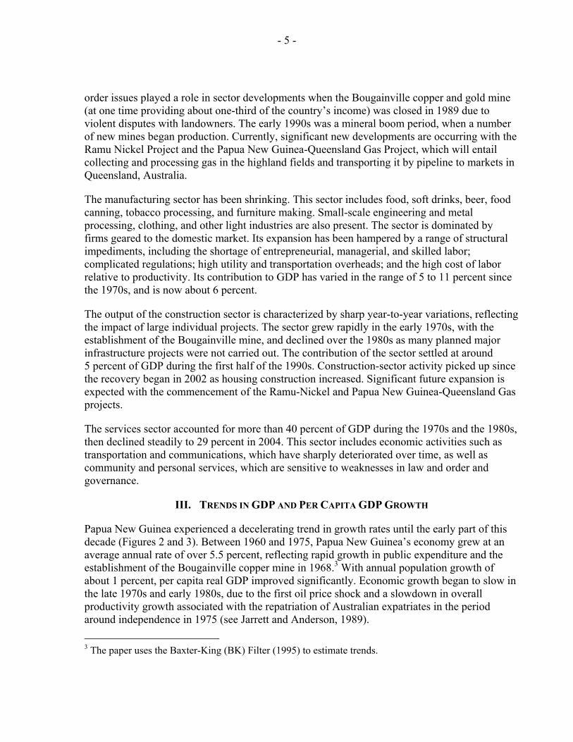
Papua New Guinea’s economy is dominated by a large, labor-intensive agricultural sector and a capital-intensive oil and minerals sector. The formal sector consists of enclave extractive industries (mining, petroleum, and logging), cash crop production, and a small, import-substituting manufacturing sector. The informal sector is largely subsistence agriculture. Over the years, Papua New Guinea’s uneven and volatile growth rates have been accompanied by structural transformation (Figure 1). Unlike the trend observed in many developing countries, the share in GDP of the primary sector, which includes the mineral sector, has increased steadily since 1975, while those of the tertiary and secondary sectors have declined. At the same time, while the share of the secondary sector generally increases over time in most mineral- and petroleum-producing countries, it has declined steadily in Papua New Guinea, an indication of the enclave nature of the extractive sector.

The importance of the agriculture sector is currently about the same as at independence, reflecting structural impediments that have deterred more rapid growth. In the 1970s, the agricultural sector (including forestry and fisheries) accounted for about 40 percent of GDP. The GDP share of agriculture declined to about 30 percent in 1985 before increasing again to about 38 percent in 2002–04, due to increases in the shares of fisheries and forestry. Both of the latter are marked by the presence of large, foreign-owned enterprises. The main agricultural sector, including the cash and subsistence crops, is dominated by small farmers and has been hurt by the deterioration of physical infrastructure and of weak law and order.

The mining sector’s share of GDP increased from negligible levels in the 1970s to about 30 percent in the early 1990s, before slipping to about 13 percent during 2003–04. The sector is overwhelmingly foreign-owned, though the government holds equity in some projects, and developments largely track events in the global mineral sector. However, domestic law-and-

- 5 -

order issues played a role in sector developments when the Bougainville copper and gold mine (at one time providing about one-third of the country’s income) was closed in 1989 due to violent disputes with landowners. The early 1990s was a mineral boom period, when a number of new mines began production. Currently, significant new developments are occurring with the Ramu Nickel Project and the Papua New Guinea-Queensland Gas Project, which will entail collecting and processing gas in the highland fields and transporting it by pipeline to markets in Queensland, Australia.

The manufacturing sector has been shrinking. This sector includes food, soft drinks, beer, food canning, tobacco processing, and furniture making. Small-scale engineering and metal processing, clothing, and other light industries are also present. The sector is dominated by firms geared to the domestic market. Its expansion has been hampered by a range of structural impediments, including the shortage of entrepreneurial, managerial, and skilled labor; complicated regulations; high utility and transportation overheads; and the high cost of labor relative to productivity. Its contribution to GDP has varied in the range of 5 to 11 percent since the 1970s, and is now about 6 percent.

The output of the construction sector is characterized by sharp year-to-year variations, reflecting the impact of large individual projects. The sector grew rapidly in the early 1970s, with the establishment of the Bougainville mine, and declined over the 1980s as many planned major infrastructure projects were not carried out. The contribution of the sector settled at around 5 percent of GDP during the first half of the 1990s. Construction-sector activity picked up since the recovery began in 2002 as housing construction increased. Significant future expansion is expected with the commencement of the Ramu-Nickel and Papua New Guinea-Queensland Gas projects.

The services sector accounted for more than 40 percent of GDP during the 1970s and the 1980s, then declined steadily to 29 percent in 2004. This sector includes economic activities such as transportation and communications, which have sharply deteriorated over time, as well as community and personal services, which are sensitive to weaknesses in law and order and governance.

III. TRENDS IN GDP AND PER CAPITA GDP GROWTH

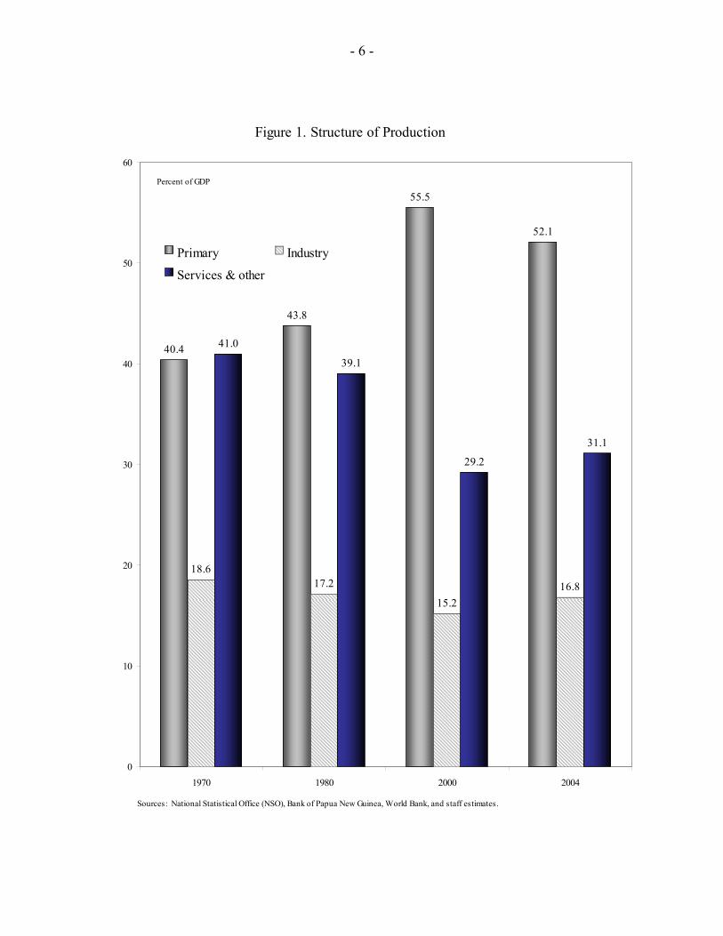
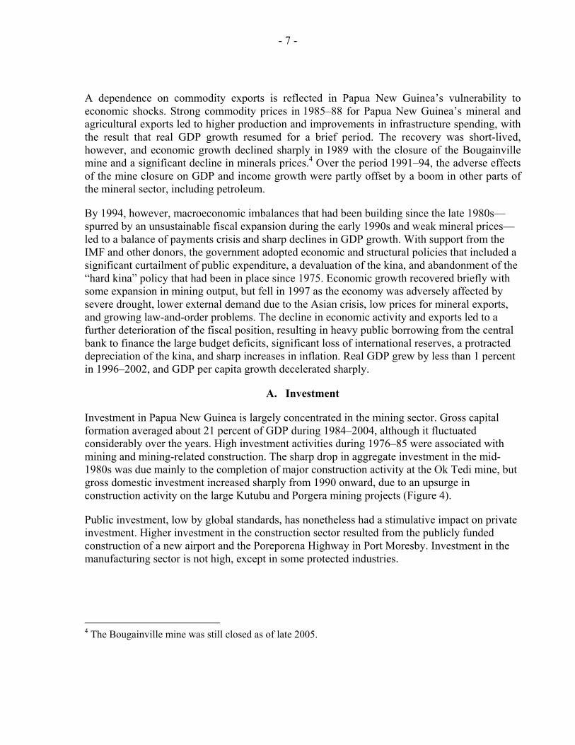
Papua New Guinea experienced a decelerating trend in growth rates until the early part of this decade (Figures 2 and 3). Between 1960 and 1975, Papua New Guinea’s economy grew at an average annual rate of over 5.5 percent, reflecting rapid growth in public expenditure and the establishment of the Bougainville copper mine in 1968.3 With annual population growth of about 1 percent, per capita real GDP improved significantly. Economic growth began to slow in the late 1970s and early 1980s, due to the first oil price shock and a slowdown in overall productivity growth associated with the repatriation of Australian expatriates in the period around independence in 1975 (see Jarrett and Anderson, 1989).

3 The paper uses the Baxter-King (BK) Filter (1995) to estimate trends.

- 6 -

Figure 1. Structure of Production

40.4

43.8

55.5

52.1

18.617.2

15.216.8

41.0

39.1

29.2

31.1

0

10

20

30

40

50

60

1970 1980 2000 2004

Primary Industry

Services & other

Percent of GDP

Sources: National Statistical Office (NSO), Bank of Papua New Guinea, World Bank, and staff estimates.

- 7 -

A dependence on commodity exports is reflected in Papua New Guinea’s vulnerability to economic shocks. Strong commodity prices in 1985–88 for Papua New Guinea’s mineral and agricultural exports led to higher production and improvements in infrastructure spending, with the result that real GDP growth resumed for a brief period. The recovery was short-lived, however, and economic growth declined sharply in 1989 with the closure of the Bougainville mine and a significant decline in minerals prices.4 Over the period 1991–94, the adverse effects of the mine closure on GDP and income growth were partly offset by a boom in other parts of the mineral sector, including petroleum.

By 1994, however, macroeconomic imbalances that had been building since the late 1980s—spurred by an unsustainable fiscal expansion during the early 1990s and weak mineral prices—led to a balance of payments crisis and sharp declines in GDP growth. With support from the IMF and other donors, the government adopted economic and structural policies that included a significant curtailment of public expenditure, a devaluation of the kina, and abandonment of the “hard kina” policy that had been in place since 1975. Economic growth recovered briefly with some expansion in mining output, but fell in 1997 as the economy was adversely affected by severe drought, lower external demand due to the Asian crisis, low prices for mineral exports, and growing law-and-order problems. The decline in economic activity and exports led to a further deterioration of the fiscal position, resulting in heavy public borrowing from the central bank to finance the large budget deficits, significant loss of international reserves, a protracted depreciation of the kina, and sharp increases in inflation. Real GDP grew by less than 1 percent in 1996–2002, and GDP per capita growth decelerated sharply.

A. Investment

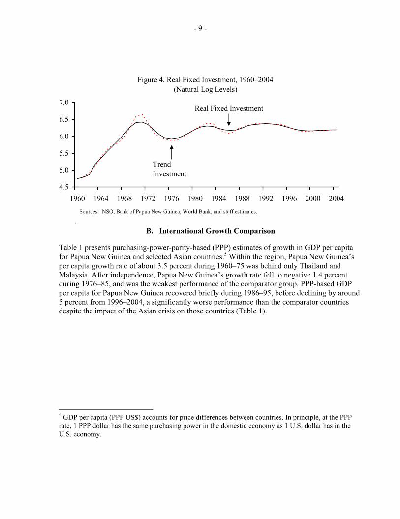
Investment in Papua New Guinea is largely concentrated in the mining sector. Gross capital formation averaged about 21 percent of GDP during 1984–2004, although it fluctuated considerably over the years. High investment activities during 1976–85 were associated with mining and mining-related construction. The sharp drop in aggregate investment in the mid-1980s was due mainly to the completion of major construction activity at the Ok Tedi mine, but gross domestic investment increased sharply from 1990 onward, due to an upsurge in construction activity on the large Kutubu and Porgera mining projects (Figure 4).

Public investment, low by global standards, has nonetheless had a stimulative impact on private investment. Higher investment in the construction sector resulted from the publicly funded construction of a new airport and the Poreporena Highway in Port Moresby. Investment in the manufacturing sector is not high, except in some protected industries.

4 The Bougainville mine was still closed as of late 2005.

- 8 -

Sources: INEGI and Fund staff estimates.

Figure 2. Actual and Trend GDP, 1960–2004(Natural Log Levels)

6.7

7.2

7.7

8.2

1960 1964 1968 1972 1976 1980 1984 1988 1992 1996 2000 2004

Trend GDP(B-K Filter)

GDP

Sources: NSO, Bank of Papua New Guinea, World Bank, and staff estimates.

Figure 3. Actual and Trend GDP Per Capita, 1960–2004(Natural Log Levels)

6.0

6.16.2

6.36.4

6.56.6

6.7

1960 1964 1968 1972 1976 1980 1984 1988 1992 1996 2000 2004

Trend (B-K Filter)GDP per capita

Sources: NSO, Bank of Papua New Guinea, World Bank, and staff estimates.

Foreign investors have played a significant role. Australia is the largest foreign investor in both mining and nonmining sectors of Papua New Guinea. Development of new mines such as OK Tedi (copper and gold), Hides (gas), Kutubu (oil), Lihir (gold), Porgera (gold), and Misima (gold) have also attracted U.S., U.K., and Canadian mining interests. Malaysia has become a significant investor in fisheries, timber, and other trade and construction subsectors. Real gross fixed capital formation fell to 13.7 percent of GDP in 1998, compared with 21 percent in 1984, due mainly to outflow of foreign capital since 1994 when macroeconomic performance declined sharply (Curtin, 2001), although it has since recovered.

- 9 -

B. International Growth Comparison

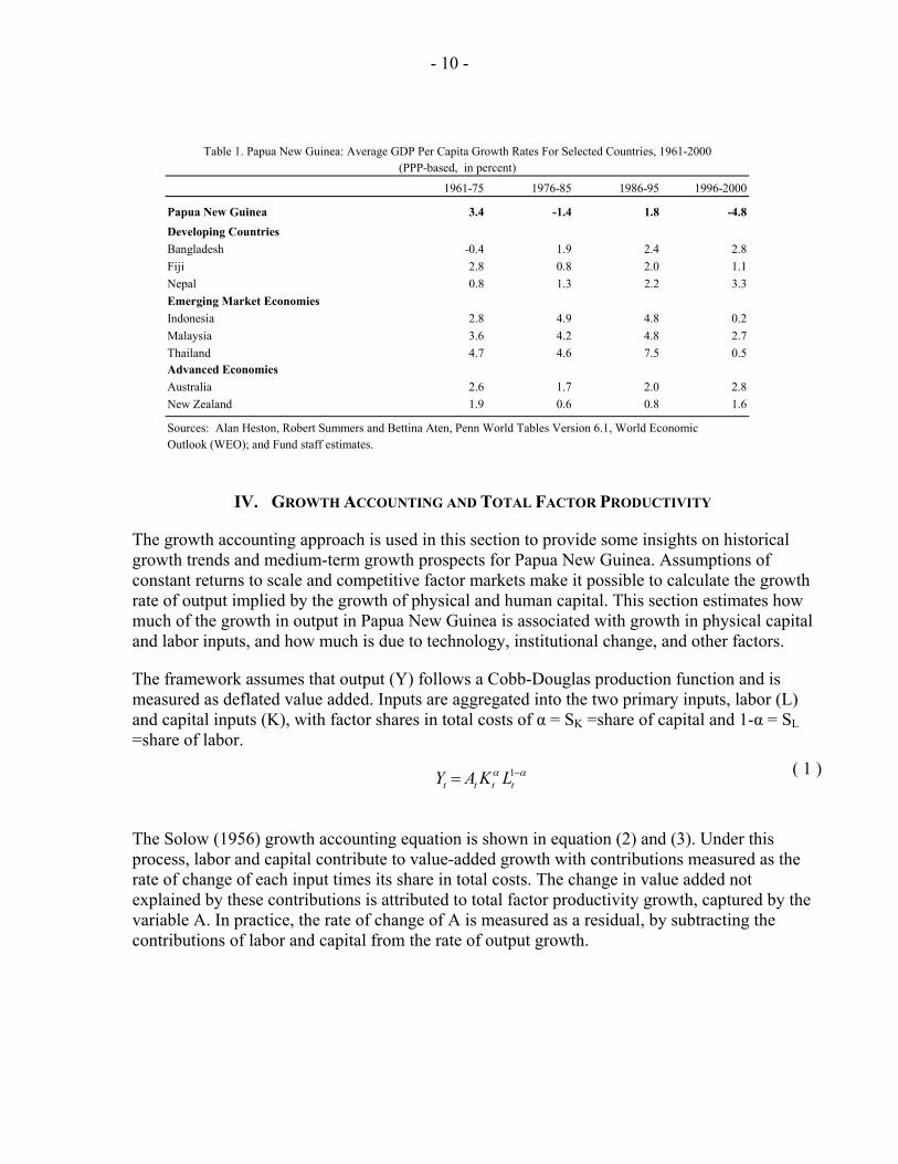
Table 1 presents purchasing-power-parity-based (PPP) estimates of growth in GDP per capita for Papua New Guinea and selected Asian countries.5 Within the region, Papua New Guinea’s per capita growth rate of about 3.5 percent during 1960–75 was behind only Thailand and Malaysia. After independence, Papua New Guinea’s growth rate fell to negative 1.4 percent during 1976–85, and was the weakest performance of the comparator group. PPP-based GDP per capita for Papua New Guinea recovered briefly during 1986–95, before declining by around 5 percent from 1996–2004, a significantly worse performance than the comparator countries despite the impact of the Asian crisis on those countries (Table 1).

5 GDP per capita (PPP US$) accounts for price differences between countries. In principle, at the PPP rate, 1 PPP dollar has the same purchasing power in the domestic economy as 1 U.S. dollar has in the U.S. economy.

Sources: INEGI and Fund staff estimates.

Figure 4. Real Fixed Investment, 1960–2004(Natural Log Levels)

4.5

5.0

5.5

6.0

6.5

7.0

1960 1964 1968 1972 1976 1980 1984 1988 1992 1996 2000 2004

Trend Investment

Real Fixed Investment

.

Sources: NSO, Bank of Papua New Guinea, World Bank, and staff estimates.

- 10 -

IV. GROWTH ACCOUNTING AND TOTAL FACTOR PRODUCTIVITY

The growth accounting approach is used in this section to provide some insights on historical growth trends and medium-term growth prospects for Papua New Guinea. Assumptions of constant returns to scale and competitive factor markets make it possible to calculate the growth rate of output implied by the growth of physical and human capital. This section estimates how much of the growth in output in Papua New Guinea is associated with growth in physical capital and labor inputs, and how much is due to technology, institutional change, and other factors.

The framework assumes that output (Y) follows a Cobb-Douglas production function and is measured as deflated value added. Inputs are aggregated into the two primary inputs, labor (L) and capital inputs (K), with factor shares in total costs of α = SK =share of capital and 1-α = SL =share of labor.

1t t t tY A K Lα α−= ( 1 )

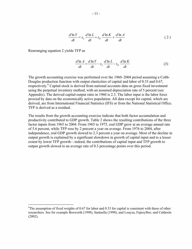
The Solow (1956) growth accounting equation is shown in equation (2) and (3). Under this process, labor and capital contribute to value-added growth with contributions measured as the rate of change of each input times its share in total costs. The change in value added not explained by these contributions is attributed to total factor productivity growth, captured by the variable A. In practice, the rate of change of A is measured as a residual, by subtracting the contributions of labor and capital from the rate of output growth.

1961-75 1976-85 1986-95 1996-2000

Papua New Guinea 3.4 -1.4 1.8 -4.8Developing CountriesBangladesh -0.4 1.9 2.4 2.8Fiji 2.8 0.8 2.0 1.1Nepal 0.8 1.3 2.2 3.3Emerging Market EconomiesIndonesia 2.8 4.9 4.8 0.2Malaysia 3.6 4.2 4.8 2.7Thailand 4.7 4.6 7.5 0.5Advanced EconomiesAustralia 2.6 1.7 2.0 2.8New Zealand 1.9 0.6 0.8 1.6

Sources: Alan Heston, Robert Summers and Bettina Aten, Penn World Tables Version 6.1, World Economic Outlook (WEO); and Fund staff estimates.

Table 1. Papua New Guinea: Average GDP Per Capita Growth Rates For Selected Countries, 1961-2000(PPP-based, in percent)

- 11 -

ln ln ln ln

L Kd Y d L d K d As s

dt dt dt dt= + + ( 2 )

Rearranging equation 2 yields TFP as

ln ln ln lnL K

d A d Y d L d Ks sdt dt dt dt

= − − (3)

The growth accounting exercise was performed over the 1960–2004 period assuming a Cobb-Douglas production function with output elasticities of capital and labor of 0.33 and 0.67, respectively.6 Capital stock is derived from national accounts data on gross fixed investment using the perpetual inventory method, with an assumed depreciation rate of 5 percent (see Appendix). The derived capital-output ratio in 1960 is 2.3. The labor input is the labor force proxied by data on the economically active population. All data except for capital, which are derived, are from International Financial Statistics (IFS) or from the National Statistical Office. TFP is derived as a residual.

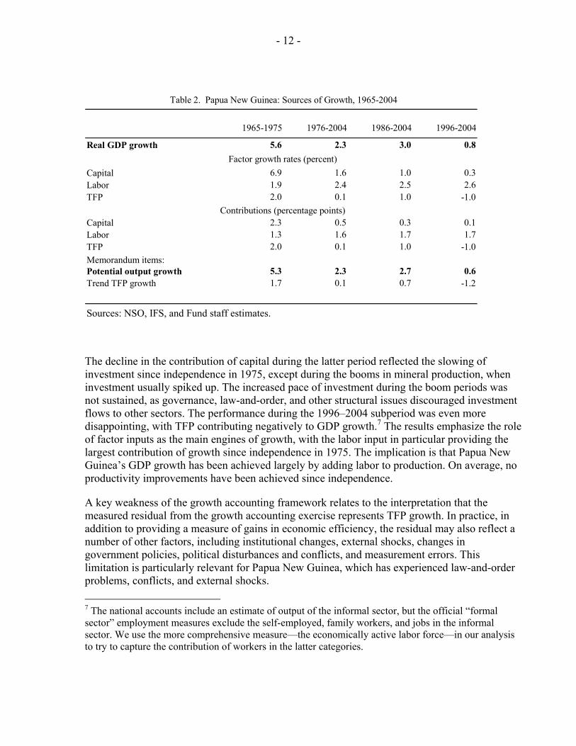
The results from the growth accounting exercise indicate that both factor accumulation and productivity contributed to GDP growth. Table 2 shows the resulting contributions of the three factor inputs from 1965 to 2004. From 1965 to 1975, real GDP grew at an average annual rate of 5.6 percent, while TFP rose by 2 percent a year on average. From 1976 to 2004, after independence, real GDP growth slowed to 2.3 percent a year on average. Most of the decline in output growth is explained by a significant slowdown in growth of capital input and to a lesser extent by lower TFP growth—indeed, the contributions of capital input and TFP growth to output growth slowed to an average rate of 0.3 percentage points over this period.

6The assumption of fixed weights of 0.67 for labor and 0.33 for capital is consistent with those of other researchers. See for example Bosworth (1998), Santaella (1998), and Loayza, Fajnzylber, and Calderón (2002).

- 12 -

The decline in the contribution of capital during the latter period reflected the slowing of investment since independence in 1975, except during the booms in mineral production, when investment usually spiked up. The increased pace of investment during the boom periods was not sustained, as governance, law-and-order, and other structural issues discouraged investment flows to other sectors. The performance during the 1996–2004 subperiod was even more disappointing, with TFP contributing negatively to GDP growth.7 The results emphasize the role of factor inputs as the main engines of growth, with the labor input in particular providing the largest contribution of growth since independence in 1975. The implication is that Papua New Guinea’s GDP growth has been achieved largely by adding labor to production. On average, no productivity improvements have been achieved since independence.

A key weakness of the growth accounting framework relates to the interpretation that the measured residual from the growth accounting exercise represents TFP growth. In practice, in addition to providing a measure of gains in economic efficiency, the residual may also reflect a number of other factors, including institutional changes, external shocks, changes in government policies, political disturbances and conflicts, and measurement errors. This limitation is particularly relevant for Papua New Guinea, which has experienced law-and-order problems, conflicts, and external shocks. 7 The national accounts include an estimate of output of the informal sector, but the official “formal sector” employment measures exclude the self-employed, family workers, and jobs in the informal sector. We use the more comprehensive measure—the economically active labor force—in our analysis to try to capture the contribution of workers in the latter categories.

Table 2. Papua New Guinea: Sources of Growth, 1965-2004

1965-1975 1976-2004 1986-2004 1996-2004

Real GDP growth 5.6 2.3 3.0 0.8

Capital 6.9 1.6 1.0 0.3Labor 1.9 2.4 2.5 2.6TFP 2.0 0.1 1.0 -1.0

Capital 2.3 0.5 0.3 0.1Labor 1.3 1.6 1.7 1.7TFP 2.0 0.1 1.0 -1.0Memorandum items: Potential output growth 5.3 2.3 2.7 0.6Trend TFP growth 1.7 0.1 0.7 -1.2

Sources: NSO, IFS, and Fund staff estimates.

Contributions (percentage points)

Factor growth rates (percent)

- 13 -

Another problem with the growth accounting framework is that it does not properly decompose growth stemming from the exploitation of natural resources or for different types of factor inputs. Due to data limitations, our analysis did not attempt to consider separately the mining and nonmining sectors nor to control for changes in the quality of human capital. There are several types of labor and capital. If data are available, aggregated factor inputs can be decomposed to measure sectoral factor inputs. For example, the aggregated figure of labor inputs can be decomposed to determine how labor quality changes affect TFP growth in a given sector. The same method can be applied for capital. However, as the necessary data on capital are not available, this paper focuses only on the adjustments for business fluctuations.

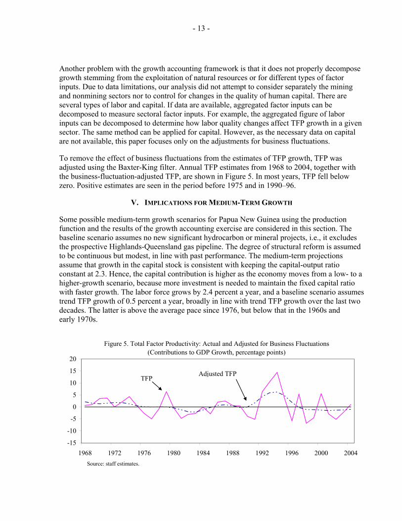
To remove the effect of business fluctuations from the estimates of TFP growth, TFP was adjusted using the Baxter-King filter. Annual TFP estimates from 1968 to 2004, together with the business-fluctuation-adjusted TFP, are shown in Figure 5. In most years, TFP fell below zero. Positive estimates are seen in the period before 1975 and in 1990–96.

V. IMPLICATIONS FOR MEDIUM-TERM GROWTH

Some possible medium-term growth scenarios for Papua New Guinea using the production function and the results of the growth accounting exercise are considered in this section. The baseline scenario assumes no new significant hydrocarbon or mineral projects, i.e., it excludes the prospective Highlands-Queensland gas pipeline. The degree of structural reform is assumed to be continuous but modest, in line with past performance. The medium-term projections assume that growth in the capital stock is consistent with keeping the capital-output ratio constant at 2.3. Hence, the capital contribution is higher as the economy moves from a low- to a higher-growth scenario, because more investment is needed to maintain the fixed capital ratio with faster growth. The labor force grows by 2.4 percent a year, and a baseline scenario assumes trend TFP growth of 0.5 percent a year, broadly in line with trend TFP growth over the last two decades. The latter is above the average pace since 1976, but below that in the 1960s and early 1970s.

Figure 5. Total Factor Productivity: Actual and Adjusted for Business Fluctuations (Contributions to GDP Growth, percentage points)

-15

-10

-5

0

5

10

15

20

1968 1972 1976 1980 1984 1988 1992 1996 2000 2004

TFPAdjusted TFP

Source: staff estimates.

- 14 -

Potential output is derived as the sum of trend TFP and the contributions of the capital and trend labor inputs.

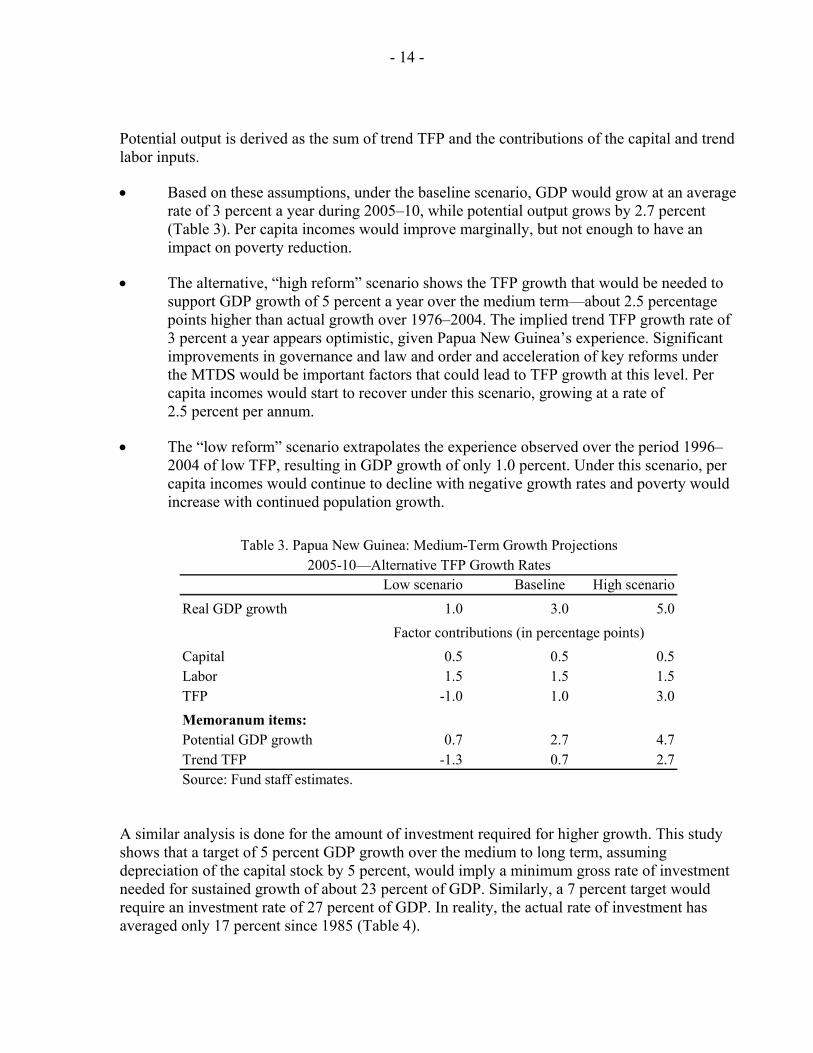
• Based on these assumptions, under the baseline scenario, GDP would grow at an average rate of 3 percent a year during 2005–10, while potential output grows by 2.7 percent (Table 3). Per capita incomes would improve marginally, but not enough to have an impact on poverty reduction.

• The alternative, “high reform” scenario shows the TFP growth that would be needed to support GDP growth of 5 percent a year over the medium term—about 2.5 percentage points higher than actual growth over 1976–2004. The implied trend TFP growth rate of 3 percent a year appears optimistic, given Papua New Guinea’s experience. Significant improvements in governance and law and order and acceleration of key reforms under the MTDS would be important factors that could lead to TFP growth at this level. Per capita incomes would start to recover under this scenario, growing at a rate of 2.5 percent per annum.

• The “low reform” scenario extrapolates the experience observed over the period 1996–2004 of low TFP, resulting in GDP growth of only 1.0 percent. Under this scenario, per capita incomes would continue to decline with negative growth rates and poverty would increase with continued population growth.

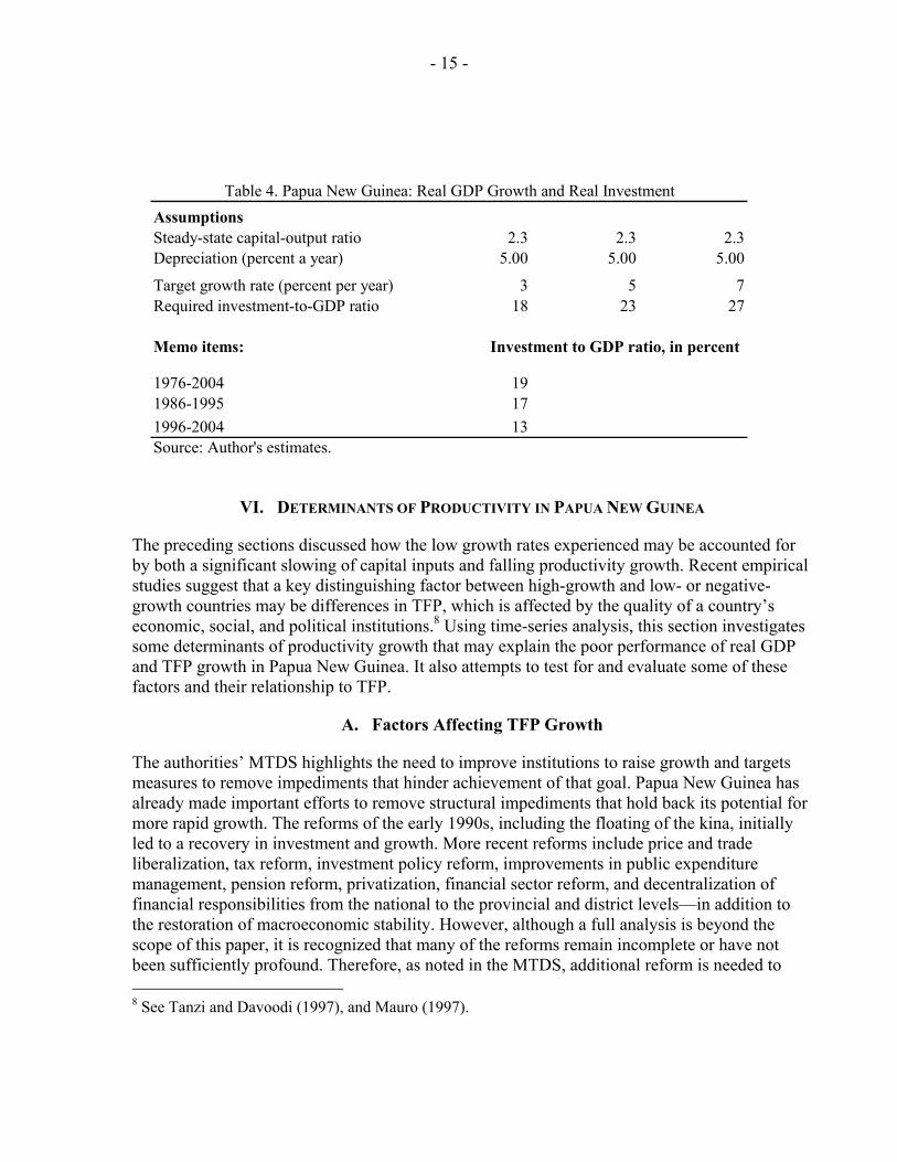
A similar analysis is done for the amount of investment required for higher growth. This study shows that a target of 5 percent GDP growth over the medium to long term, assuming depreciation of the capital stock by 5 percent, would imply a minimum gross rate of investment needed for sustained growth of about 23 percent of GDP. Similarly, a 7 percent target would require an investment rate of 27 percent of GDP. In reality, the actual rate of investment has averaged only 17 percent since 1985 (Table 4).

Low scenario Baseline High scenario

Real GDP growth 1.0 3.0 5.0

Capital 0.5 0.5 0.5Labor 1.5 1.5 1.5TFP -1.0 1.0 3.0Memoranum items:Potential GDP growth 0.7 2.7 4.7Trend TFP -1.3 0.7 2.7Source: Fund staff estimates.

Table 3. Papua New Guinea: Medium-Term Growth Projections2005-10—Alternative TFP Growth Rates

Factor contributions (in percentage points)

- 15 -

VI. DETERMINANTS OF PRODUCTIVITY IN PAPUA NEW GUINEA

The preceding sections discussed how the low growth rates experienced may be accounted for by both a significant slowing of capital inputs and falling productivity growth. Recent empirical studies suggest that a key distinguishing factor between high-growth and low- or negative-growth countries may be differences in TFP, which is affected by the quality of a country’s economic, social, and political institutions.8 Using time-series analysis, this section investigates some determinants of productivity growth that may explain the poor performance of real GDP and TFP growth in Papua New Guinea. It also attempts to test for and evaluate some of these factors and their relationship to TFP.

A. Factors Affecting TFP Growth

The authorities’ MTDS highlights the need to improve institutions to raise growth and targets measures to remove impediments that hinder achievement of that goal. Papua New Guinea has already made important efforts to remove structural impediments that hold back its potential for more rapid growth. The reforms of the early 1990s, including the floating of the kina, initially led to a recovery in investment and growth. More recent reforms include price and trade liberalization, tax reform, investment policy reform, improvements in public expenditure management, pension reform, privatization, financial sector reform, and decentralization of financial responsibilities from the national to the provincial and district levels—in addition to the restoration of macroeconomic stability. However, although a full analysis is beyond the scope of this paper, it is recognized that many of the reforms remain incomplete or have not been sufficiently profound. Therefore, as noted in the MTDS, additional reform is needed to 8 See Tanzi and Davoodi (1997), and Mauro (1997).

AssumptionsSteady-state capital-output ratio 2.3 2.3 2.3Depreciation (percent a year) 5.00 5.00 5.00

Target growth rate (percent per year) 3 5 7Required investment-to-GDP ratio 18 23 27

Memo items: Investment to GDP ratio, in percent

1976-2004 191986-1995 171996-2004 13Source: Author's estimates.

Table 4. Papua New Guinea: Real GDP Growth and Real Investment

- 16 -

bring growth rates up to the higher level required to sustain improvements in per capita GDP and to reduce poverty. The following discussion highlights several key areas for further reform.

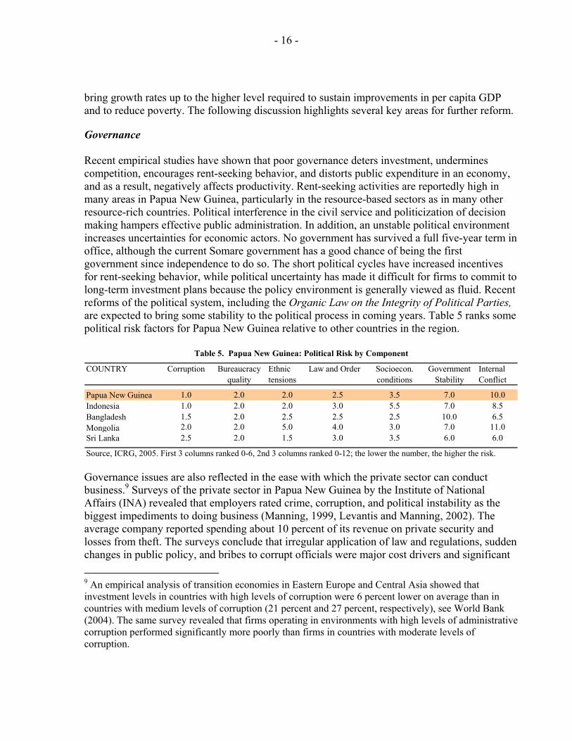
Governance Recent empirical studies have shown that poor governance deters investment, undermines competition, encourages rent-seeking behavior, and distorts public expenditure in an economy, and as a result, negatively affects productivity. Rent-seeking activities are reportedly high in many areas in Papua New Guinea, particularly in the resource-based sectors as in many other resource-rich countries. Political interference in the civil service and politicization of decision making hampers effective public administration. In addition, an unstable political environment increases uncertainties for economic actors. No government has survived a full five-year term in office, although the current Somare government has a good chance of being the first government since independence to do so. The short political cycles have increased incentives for rent-seeking behavior, while political uncertainty has made it difficult for firms to commit to long-term investment plans because the policy environment is generally viewed as fluid. Recent reforms of the political system, including the Organic Law on the Integrity of Political Parties, are expected to bring some stability to the political process in coming years. Table 5 ranks some political risk factors for Papua New Guinea relative to other countries in the region.

COUNTRY Corruption Bureaucracy quality

Ethnic tensions

Law and Order Socioecon. conditions

Government Stability

Internal Conflict

Papua New Guinea 1.0 2.0 2.0 2.5 3.5 7.0 10.0Indonesia 1.0 2.0 2.0 3.0 5.5 7.0 8.5Bangladesh 1.5 2.0 2.5 2.5 2.5 10.0 6.5Mongolia 2.0 2.0 5.0 4.0 3.0 7.0 11.0Sri Lanka 2.5 2.0 1.5 3.0 3.5 6.0 6.0

Table 5. Papua New Guinea: Political Risk by Component

Source, ICRG, 2005. First 3 columns ranked 0-6, 2nd 3 columns ranked 0-12; the lower the number, the higher the risk.

Governance issues are also reflected in the ease with which the private sector can conduct business.9 Surveys of the private sector in Papua New Guinea by the Institute of National Affairs (INA) revealed that employers rated crime, corruption, and political instability as the biggest impediments to doing business (Manning, 1999, Levantis and Manning, 2002). The average company reported spending about 10 percent of its revenue on private security and losses from theft. The surveys conclude that irregular application of law and regulations, sudden changes in public policy, and bribes to corrupt officials were major cost drivers and significant 9 An empirical analysis of transition economies in Eastern Europe and Central Asia showed that investment levels in countries with high levels of corruption were 6 percent lower on average than in countries with medium levels of corruption (21 percent and 27 percent, respectively), see World Bank (2004). The same survey revealed that firms operating in environments with high levels of administrative corruption performed significantly more poorly than firms in countries with moderate levels of corruption.

- 17 -

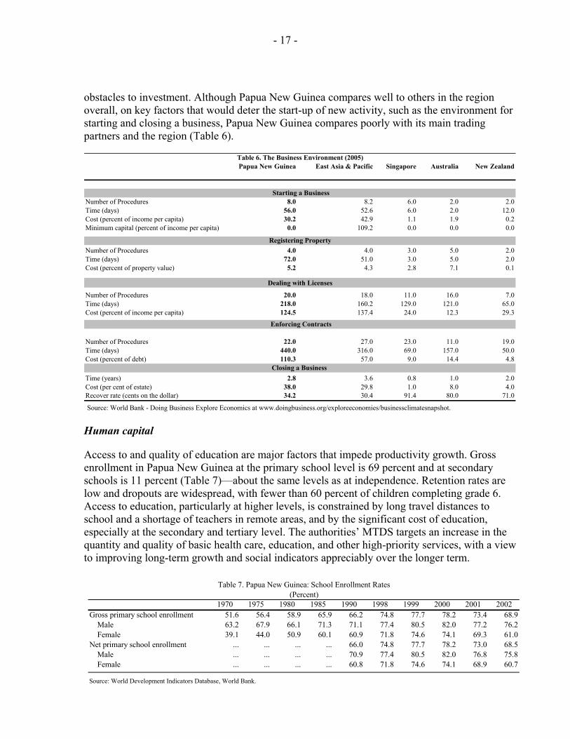
obstacles to investment. Although Papua New Guinea compares well to others in the region overall, on key factors that would deter the start-up of new activity, such as the environment for starting and closing a business, Papua New Guinea compares poorly with its main trading partners and the region (Table 6).

Papua New Guinea East Asia & Pacific Singapore Australia New Zealand

Number of Procedures 8.0 8.2 6.0 2.0 2.0Time (days) 56.0 52.6 6.0 2.0 12.0Cost (percent of income per capita) 30.2 42.9 1.1 1.9 0.2Minimum capital (percent of income per capita) 0.0 109.2 0.0 0.0 0.0

Number of Procedures 4.0 4.0 3.0 5.0 2.0Time (days) 72.0 51.0 3.0 5.0 2.0Cost (percent of property value) 5.2 4.3 2.8 7.1 0.1

Number of Procedures 20.0 18.0 11.0 16.0 7.0Time (days) 218.0 160.2 129.0 121.0 65.0Cost (percent of income per capita) 124.5 137.4 24.0 12.3 29.3

Number of Procedures 22.0 27.0 23.0 11.0 19.0Time (days) 440.0 316.0 69.0 157.0 50.0Cost (percent of debt) 110.3 57.0 9.0 14.4 4.8

Time (years) 2.8 3.6 0.8 1.0 2.0Cost (per cent of estate) 38.0 29.8 1.0 8.0 4.0Recover rate (cents on the dollar) 34.2 30.4 91.4 80.0 71.0

Source: World Bank - Doing Business Explore Economics at www.doingbusiness.org/exploreeconomies/businessclimatesnapshot.

Closing a Business

Starting a Business

Registering Property

Dealing with Licenses

Enforcing Contracts

Table 6. The Business Environment (2005)

Human capital

Access to and quality of education are major factors that impede productivity growth. Gross enrollment in Papua New Guinea at the primary school level is 69 percent and at secondary schools is 11 percent (Table 7)—about the same levels as at independence. Retention rates are low and dropouts are widespread, with fewer than 60 percent of children completing grade 6. Access to education, particularly at higher levels, is constrained by long travel distances to school and a shortage of teachers in remote areas, and by the significant cost of education, especially at the secondary and tertiary level. The authorities’ MTDS targets an increase in the quantity and quality of basic health care, education, and other high-priority services, with a view to improving long-term growth and social indicators appreciably over the longer term.

1970 1975 1980 1985 1990 1998 1999 2000 2001 2002Gross primary school enrollment 51.6 56.4 58.9 65.9 66.2 74.8 77.7 78.2 73.4 68.9 Male 63.2 67.9 66.1 71.3 71.1 77.4 80.5 82.0 77.2 76.2 Female 39.1 44.0 50.9 60.1 60.9 71.8 74.6 74.1 69.3 61.0Net primary school enrollment ... ... ... ... 66.0 74.8 77.7 78.2 73.0 68.5 Male ... ... ... ... 70.9 77.4 80.5 82.0 76.8 75.8 Female ... ... ... ... 60.8 71.8 74.6 74.1 68.9 60.7

Source: World Development Indicators Database, World Bank.

Table 7. Papua New Guinea: School Enrollment Rates(Percent)

- 18 -

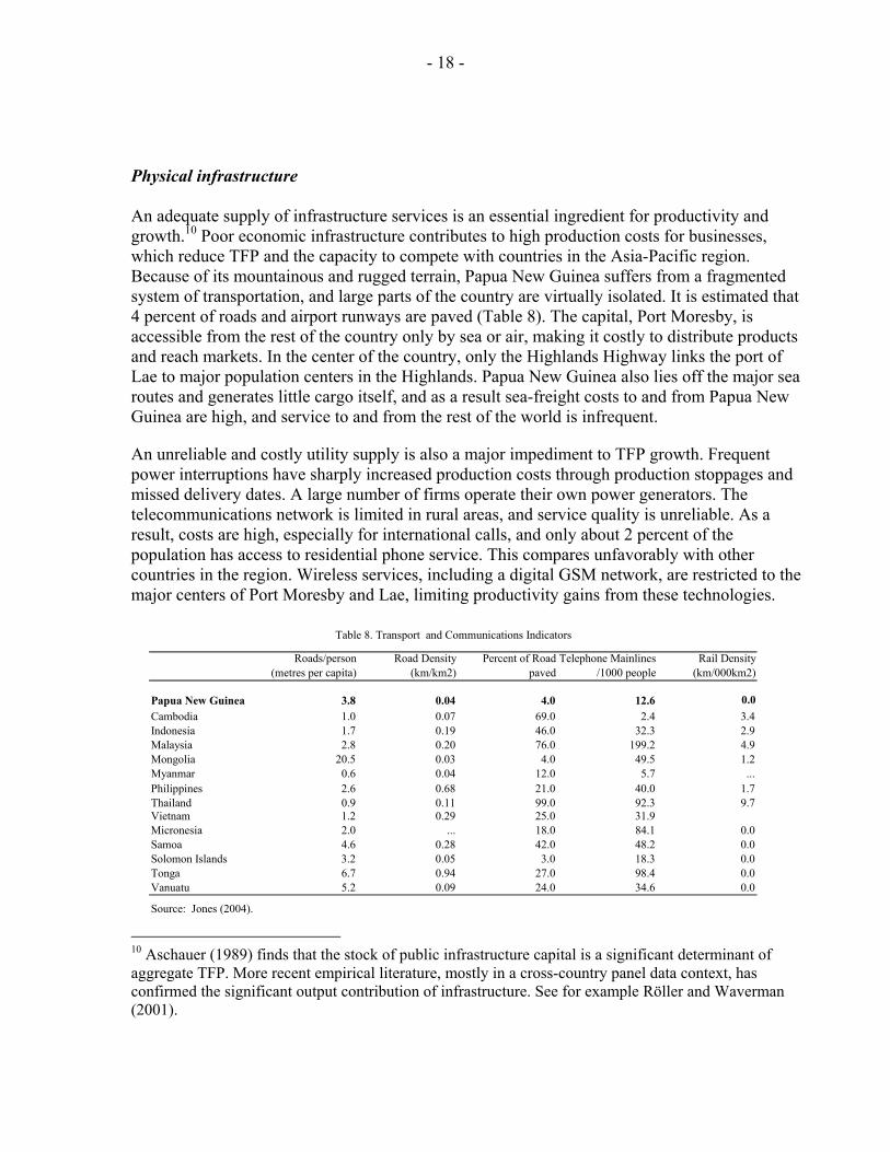
Physical infrastructure An adequate supply of infrastructure services is an essential ingredient for productivity and growth.10 Poor economic infrastructure contributes to high production costs for businesses, which reduce TFP and the capacity to compete with countries in the Asia-Pacific region. Because of its mountainous and rugged terrain, Papua New Guinea suffers from a fragmented system of transportation, and large parts of the country are virtually isolated. It is estimated that 4 percent of roads and airport runways are paved (Table 8). The capital, Port Moresby, is accessible from the rest of the country only by sea or air, making it costly to distribute products and reach markets. In the center of the country, only the Highlands Highway links the port of Lae to major population centers in the Highlands. Papua New Guinea also lies off the major sea routes and generates little cargo itself, and as a result sea-freight costs to and from Papua New Guinea are high, and service to and from the rest of the world is infrequent.

An unreliable and costly utility supply is also a major impediment to TFP growth. Frequent power interruptions have sharply increased production costs through production stoppages and missed delivery dates. A large number of firms operate their own power generators. The telecommunications network is limited in rural areas, and service quality is unreliable. As a result, costs are high, especially for international calls, and only about 2 percent of the population has access to residential phone service. This compares unfavorably with other countries in the region. Wireless services, including a digital GSM network, are restricted to the major centers of Port Moresby and Lae, limiting productivity gains from these technologies.

10 Aschauer (1989) finds that the stock of public infrastructure capital is a significant determinant of aggregate TFP. More recent empirical literature, mostly in a cross-country panel data context, has confirmed the significant output contribution of infrastructure. See for example Röller and Waverman (2001).

Roads/person (metres per capita)

Road Density (km/km2)

Percent of Road paved

Telephone Mainlines /1000 people

Rail Density (km/000km2)

Papua New Guinea 3.8 0.04 4.0 12.6 0.0Cambodia 1.0 0.07 69.0 2.4 3.4Indonesia 1.7 0.19 46.0 32.3 2.9Malaysia 2.8 0.20 76.0 199.2 4.9Mongolia 20.5 0.03 4.0 49.5 1.2Myanmar 0.6 0.04 12.0 5.7 ...Philippines 2.6 0.68 21.0 40.0 1.7Thailand 0.9 0.11 99.0 92.3 9.7Vietnam 1.2 0.29 25.0 31.9Micronesia 2.0 ... 18.0 84.1 0.0Samoa 4.6 0.28 42.0 48.2 0.0Solomon Islands 3.2 0.05 3.0 18.3 0.0Tonga 6.7 0.94 27.0 98.4 0.0Vanuatu 5.2 0.09 24.0 34.6 0.0

Source: Jones (2004).

Table 8. Transport and Communications Indicators

- 19 -

B. Empirical Estimation11

Many factors may affect TFP growth directly and indirectly. In this study, however, only those factors for which data are available are included in the empirical analysis. These include macroeconomic stability proxied by the inflation variable; technology transfer and governance (proxied by foreign direct investment); and enrollment rates to capture improvements in human capital.12 The methodology employed in this paper uses unit root and Johansen’s cointegration tests followed by a vector error correction model and variance decomposition to examine the dynamic relationships among variables. The first step requires that the unit root test be conducted in order to determine whether the series are nonstationary in levels and stationary in first differences, that is, integrated of order one. The second step is to use the cointegration test in order to determine whether those six nonstationary series have common long-run relationships. There are many possible tests for cointegration, the most general of them is the multivariate test based on the autoregressive representation discussed in Johansen (1988, 1992) and Johansen and Juselius (1990). The Johansen maximum likelihood method provides two different likelihood ratio tests, the trace test and the maximum eigenvalue test, in order to determine the number of cointegrating vectors. The finding of the presence of cointegration paves the way for using the vector error correction model.

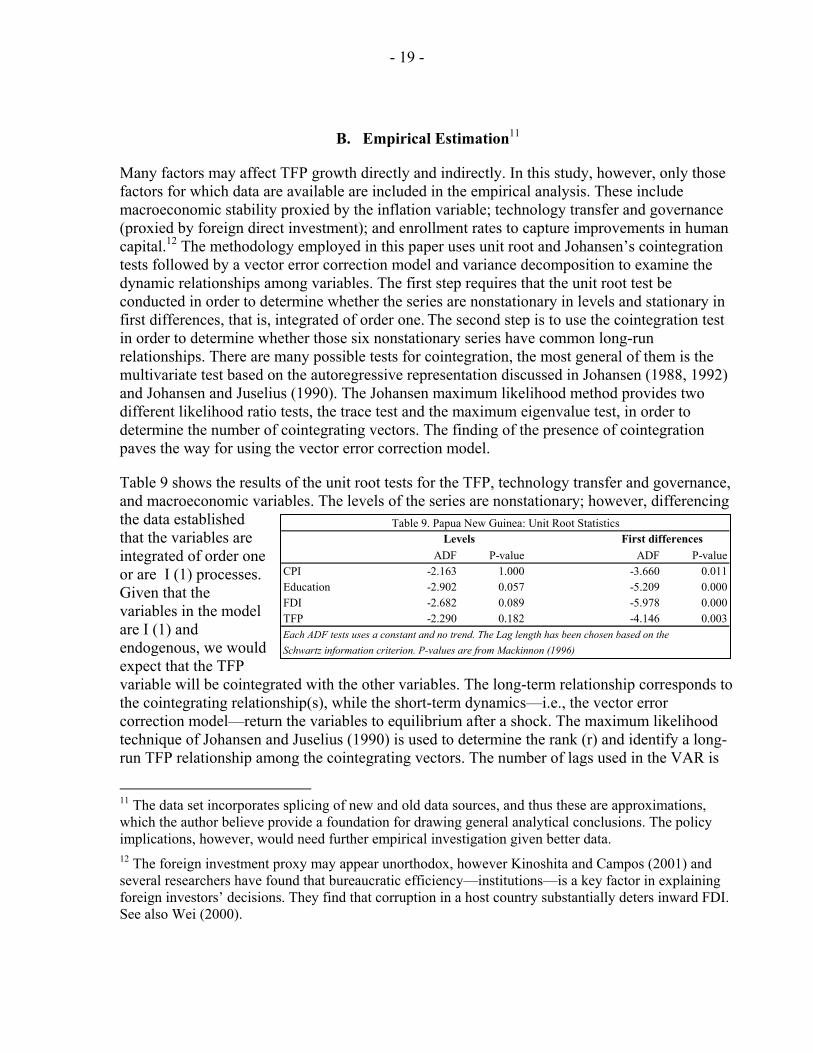
Table 9 shows the results of the unit root tests for the TFP, technology transfer and governance, and macroeconomic variables. The levels of the series are nonstationary; however, differencing the data established that the variables are integrated of order one or are I (1) processes. Given that the variables in the model are I (1) and endogenous, we would expect that the TFP variable will be cointegrated with the other variables. The long-term relationship corresponds to the cointegrating relationship(s), while the short-term dynamics—i.e., the vector error correction model—return the variables to equilibrium after a shock. The maximum likelihood technique of Johansen and Juselius (1990) is used to determine the rank (r) and identify a long-run TFP relationship among the cointegrating vectors. The number of lags used in the VAR is

11 The data set incorporates splicing of new and old data sources, and thus these are approximations, which the author believe provide a foundation for drawing general analytical conclusions. The policy implications, however, would need further empirical investigation given better data. 12 The foreign investment proxy may appear unorthodox, however Kinoshita and Campos (2001) and several researchers have found that bureaucratic efficiency—institutions—is a key factor in explaining foreign investors’ decisions. They find that corruption in a host country substantially deters inward FDI. See also Wei (2000).

ADF P-value ADF P-valueCPI -2.163 1.000 -3.660 0.011Education -2.902 0.057 -5.209 0.000FDI -2.682 0.089 -5.978 0.000TFP -2.290 0.182 -4.146 0.003Each ADF tests uses a constant and no trend. The Lag length has been chosen based on theSchwartz information criterion. P-values are from Mackinnon (1996)

First differencesLevelsTable 9. Papua New Guinea: Unit Root Statistics

- 20 -

based on the evidence provided by both likelihood ratio tests. The null hypothesis of no cointegration was rejected using both the λ-max (maximum eigenvalue statistics) and trace tests, in favor of one cointegrating relationship. Both tests indicate one cointegrating vector at the 5 percent level. We then consider a dynamic vector error correction model to capture the short-run dynamics of variables in the system. The results are presented in Table 10.

Hypothesized Trace 5 percentNo. of CE(s) Eigenvalue Statistic Critical Value P-value

None * 0.731 62.678 47.856 0.001At most 1 0.526 27.212 29.797 0.096At most 2 0.196 7.031 15.494 0.574At most 3 0.041 1.133 3.841 0.287

The cointegrating test uses an intercept but no trend in the cointegration equation. The minimum value of the Schwartzcriterion suggests the optimal lag is equal to zero for the Johanson cointegration test. Trace test indicates 1cointegrating equatio at the 0.05 level.* denotes rejection of the hypothesis at the 5 percent levels.**MacKinnon-Haug-Michelis (1999) p-values.

Table 10. Papua New Guinea: Johansen (Trace) Cointegration Test

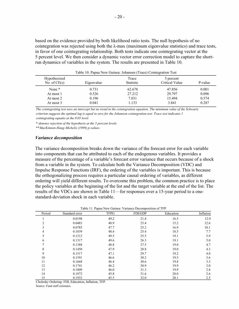
Variance decomposition The variance decomposition breaks down the variance of the forecast error for each variable into components that can be attributed to each of the endogenous variables. It provides a measure of the percentage of a variable’s forecast error variance that occurs because of a shock from a variable in the system. To calculate both the Variance Decomposition (VDC) and Impulse Response Functions (IRF), the ordering of the variables is important. This is because the orthogonalizing process requires a particular causal ordering of variables, as different ordering will yield different results. To overcome this problem, the common practice is to place the policy variables at the beginning of the list and the target variable at the end of the list. The results of the VDCs are shown in Table 11—for responses over a 15-year period to a one-standard-deviation shock in each variable.

Period Standard error TFPG FDI/GDP Education Inflation1 0.0198 49.2 21.4 16.5 12.92 0.0483 48.9 23.4 15.2 12.63 0.0785 47.7 25.2 16.9 10.14 0.1039 48.4 25.4 18.5 7.75 0.1212 49.5 25.5 19.1 5.96 0.1317 49.6 26.3 19.1 5.07 0.1388 48.8 27.5 19.0 4.78 0.1450 47.9 28.8 19.0 4.39 0.1517 47.1 29.7 19.2 4.010 0.1591 46.6 30.2 19.5 3.611 0.1668 46.4 30.6 19.8 3.312 0.1741 46.2 30.9 19.9 3.013 0.1809 46.0 31.3 19.9 2.814 0.1872 45.8 31.6 20.0 2.615 0.1933 45.5 32.0 20.1 2.5

Cholesky Ordering: FDI, Education, Inflation, TFP.Source: Fund staff estimates.

Table 11. Papua New Guinea: Variance Decomposition of TFP

- 21 -

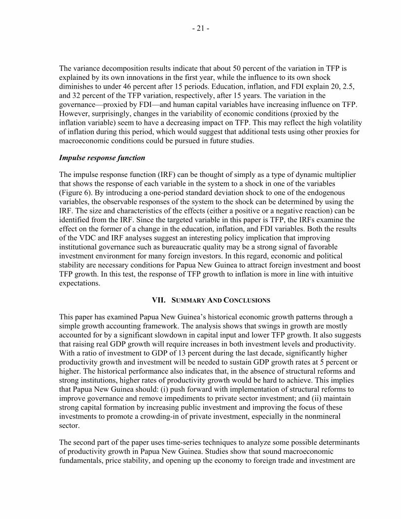
The variance decomposition results indicate that about 50 percent of the variation in TFP is explained by its own innovations in the first year, while the influence to its own shock diminishes to under 46 percent after 15 periods. Education, inflation, and FDI explain 20, 2.5, and 32 percent of the TFP variation, respectively, after 15 years. The variation in the governance—proxied by FDI—and human capital variables have increasing influence on TFP. However, surprisingly, changes in the variability of economic conditions (proxied by the inflation variable) seem to have a decreasing impact on TFP. This may reflect the high volatility of inflation during this period, which would suggest that additional tests using other proxies for macroeconomic conditions could be pursued in future studies.

Impulse response function

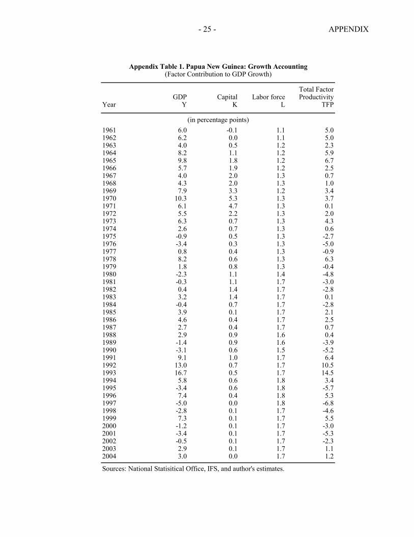
The impulse response function (IRF) can be thought of simply as a type of dynamic multiplier that shows the response of each variable in the system to a shock in one of the variables (Figure 6). By introducing a one-period standard deviation shock to one of the endogenous variables, the observable responses of the system to the shock can be determined by using the IRF. The size and characteristics of the effects (either a positive or a negative reaction) can be identified from the IRF. Since the targeted variable in this paper is TFP, the IRFs examine the effect on the former of a change in the education, inflation, and FDI variables. Both the results of the VDC and IRF analyses suggest an interesting policy implication that improving institutional governance such as bureaucratic quality may be a strong signal of favorable investment environment for many foreign investors. In this regard, economic and political stability are necessary conditions for Papua New Guinea to attract foreign investment and boost TFP growth. In this test, the response of TFP growth to inflation is more in line with intuitive expectations.

VII. SUMMARY AND CONCLUSIONS

This paper has examined Papua New Guinea’s historical economic growth patterns through a simple growth accounting framework. The analysis shows that swings in growth are mostly accounted for by a significant slowdown in capital input and lower TFP growth. It also suggests that raising real GDP growth will require increases in both investment levels and productivity. With a ratio of investment to GDP of 13 percent during the last decade, significantly higher productivity growth and investment will be needed to sustain GDP growth rates at 5 percent or higher. The historical performance also indicates that, in the absence of structural reforms and strong institutions, higher rates of productivity growth would be hard to achieve. This implies that Papua New Guinea should: (i) push forward with implementation of structural reforms to improve governance and remove impediments to private sector investment; and (ii) maintain strong capital formation by increasing public investment and improving the focus of these investments to promote a crowding-in of private investment, especially in the nonmineral sector.

The second part of the paper uses time-series techniques to analyze some possible determinants of productivity growth in Papua New Guinea. Studies show that sound macroeconomic fundamentals, price stability, and opening up the economy to foreign trade and investment are

- 22 -

critical factors affecting TFP growth. The results of the empirical estimation conducted for Papua New Guinea are consistent with these findings. In particular, the results suggest that factors that can positively influence real GDP and productivity growth in Papua New Guinea include, among others, a stable macroeconomic environment and policies, higher levels of investment and technology transfer, and better public policies to reduce corruption and improve the quality of public institutions.

- 23 -

Figure 6. Response of TFP Growth to a One S.D. Cholesky Shock

Source: Author's estimates.

Response of TFP Growth to TFP Growth

-0.04

-0.02

0

0.02

0.04

0.06

0.08

1 2 3 4 5 6 7 8 9 10 11 12 13 14 15

Response of TFP Growth to FDIGDP

-0.04

-0.02

0.00

0.02

0.04

0.06

0.08

1 2 3 4 5 6 7 8 9 10 11 12 13 14 15

Response of TFP Growth to Education

-0.04

-0.02

0.00

0.02

0.04

0.06

0.08

1 2 3 4 5 6 7 8 9 10 11 12 13 14 15

Response of TFP Growth to CPI

-0.04

-0.02

0.00

0.02

0.04

0.06

0.08

1 2 3 4 5 6 7 8 9 10 11 12 13 14 15

- 24 - APPENDIX

CALCULATING CAPITAL STOCK

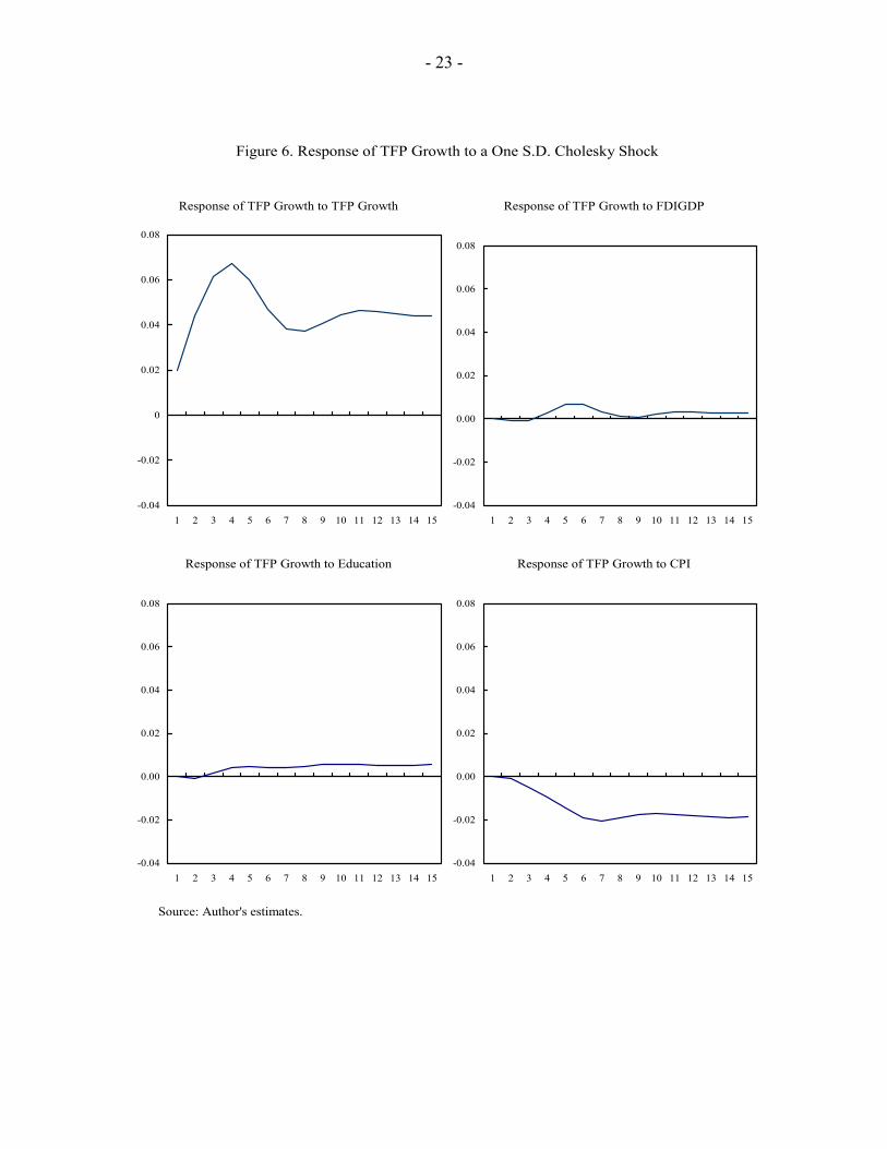
Data on capital stock (K) are not published and had to be estimated. The most common method of calculation is the so-called permanent inventory method, which can be described briefly with the equation:

1(1 )t t tK I K −= + − ∂ ( 1 )

Equation (1) allows for recursive substitution back in time and also in the future. For example, if we rewrite the formula for period (t − 1), we have:

1 1 2(1 )t t tK I K− − −= + − ∂ ( 2 )

Substituting (2) in (1) we get:

21 2(1 ) (1 )t t t tK I I K− −= + − ∂ + − ∂ ( 3 )

The process can be replicated back to some definite time so that in general,

1

10

(1 ) (1 )n

n i nt t i t n

iK I K

−−

− − −=

= − ∂ + − ∂∑ ( 4 )

where n is the definite time under consideration, from which we take the initial capital stock. It can be shown that even with n → ∞, the expression for the amortized value of the initial capital stock never becomes exactly zero, i.e. this way of calculation implies “eternal life” for some part of the capital stock. For the purposes of our analysis, the capital has to have a finite life—i.e., to depreciate entirely for a finite number of years. The latter is also required from a practical point of view, because after a specified period of time the capital stock loses its ability to create new value. For this reason the following variant of equation (4) has been used here to the calculation of the capital stock:

1

10

(1 ) (1 )n

t t i t ni

K i I n K−

− − −=

= − ∂ + − ∂∑ ( 5 )

Equation (5) implies a constant and an even (linear) reduction of the value of the initial capital, as well as of the value of investments that are made between the initial and the present moment. Also, in such a way we allow for full depreciation of a capital unit for 1/δ periods.

- 25 - APPENDIX

Total FactorGDP Capital Labor force Productivity

Year Y K L TFP

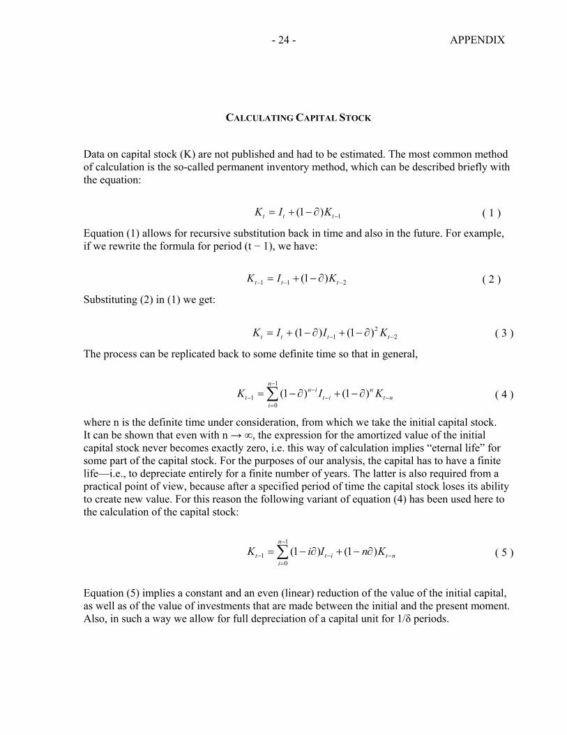
1961 6.0 -0.1 1.1 5.01962 6.2 0.0 1.1 5.01963 4.0 0.5 1.2 2.31964 8.2 1.1 1.2 5.91965 9.8 1.8 1.2 6.71966 5.7 1.9 1.2 2.51967 4.0 2.0 1.3 0.71968 4.3 2.0 1.3 1.01969 7.9 3.3 1.2 3.41970 10.3 5.3 1.3 3.71971 6.1 4.7 1.3 0.11972 5.5 2.2 1.3 2.01973 6.3 0.7 1.3 4.31974 2.6 0.7 1.3 0.61975 -0.9 0.5 1.3 -2.71976 -3.4 0.3 1.3 -5.01977 0.8 0.4 1.3 -0.91978 8.2 0.6 1.3 6.31979 1.8 0.8 1.3 -0.41980 -2.3 1.1 1.4 -4.81981 -0.3 1.1 1.7 -3.01982 0.4 1.4 1.7 -2.81983 3.2 1.4 1.7 0.11984 -0.4 0.7 1.7 -2.81985 3.9 0.1 1.7 2.11986 4.6 0.4 1.7 2.51987 2.7 0.4 1.7 0.71988 2.9 0.9 1.6 0.41989 -1.4 0.9 1.6 -3.91990 -3.1 0.6 1.5 -5.21991 9.1 1.0 1.7 6.41992 13.0 0.7 1.7 10.51993 16.7 0.5 1.7 14.51994 5.8 0.6 1.8 3.41995 -3.4 0.6 1.8 -5.71996 7.4 0.4 1.8 5.31997 -5.0 0.0 1.8 -6.81998 -2.8 0.1 1.7 -4.61999 7.3 0.1 1.7 5.52000 -1.2 0.1 1.7 -3.02001 -3.4 0.1 1.7 -5.32002 -0.5 0.1 1.7 -2.32003 2.9 0.1 1.7 1.12004 3.0 0.0 1.7 1.2

Sources: National Statisitical Office, IFS, and author's estimates.

Appendix Table 1. Papua New Guinea: Growth Accounting(Factor Contribution to GDP Growth)

(in percentage points)

- 26 - APPENDIX

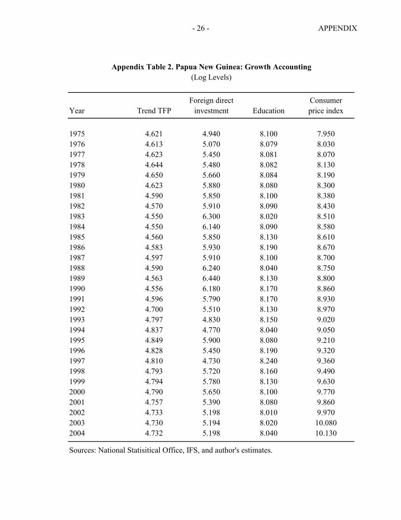
Foreign direct ConsumerYear Trend TFP investment Education price index

1975 4.621 4.940 8.100 7.9501976 4.613 5.070 8.079 8.0301977 4.623 5.450 8.081 8.0701978 4.644 5.480 8.082 8.1301979 4.650 5.660 8.084 8.1901980 4.623 5.880 8.080 8.3001981 4.590 5.850 8.100 8.3801982 4.570 5.910 8.090 8.4301983 4.550 6.300 8.020 8.5101984 4.550 6.140 8.090 8.5801985 4.560 5.850 8.130 8.6101986 4.583 5.930 8.190 8.6701987 4.597 5.910 8.100 8.7001988 4.590 6.240 8.040 8.7501989 4.563 6.440 8.130 8.8001990 4.556 6.180 8.170 8.8601991 4.596 5.790 8.170 8.9301992 4.700 5.510 8.130 8.9701993 4.797 4.830 8.150 9.0201994 4.837 4.770 8.040 9.0501995 4.849 5.900 8.080 9.2101996 4.828 5.450 8.190 9.3201997 4.810 4.730 8.240 9.3601998 4.793 5.720 8.160 9.4901999 4.794 5.780 8.130 9.6302000 4.790 5.650 8.100 9.7702001 4.757 5.390 8.080 9.8602002 4.733 5.198 8.010 9.9702003 4.730 5.194 8.020 10.0802004 4.732 5.198 8.040 10.130

Sources: National Statisitical Office, IFS, and author's estimates.

Appendix Table 2. Papua New Guinea: Growth Accounting(Log Levels)

- 27 -

REFERENCES

Aschauer, David, 1989, “Is Public Expenditure Productive?” Journal of Monetary Economics, Vol. 23, pp. 177–200. Bank of Hawaii, 2001, Papua New Guinea Economic Report (Honolulu, Hawaii). Baxter, Marianne, and Robert King, 1995, “Measuring Business Cycles: Approximate Band- Pass Filters for Economic Time Series,” The Review of Economics and Statistics, Vol. 81, pp. 575-93. Bosworth, Barry, 1998, “Productivity Growth in Mexico,” Background paper prepared for a World Bank Project on productivity growth in Mexico, Mexico: Enhancing Factor Productivity Growth, Report No. 17392-ME, Country Economic Memorandum (Washington: World Bank). Collins, Susan, and Barry Bosworth, 1996, “Economic Growth in East Asia: Accumulation Versus Assimilation,” Brookings Papers on Economic Activity, Vol. 2, pp. 135–204. Curtin, Tim, 2001, “Could Have Done Better: An Update on Economic Developments in Papua New Guinea Since 1995” (Unpublished; www.geocities.com/CapitolHill/Senate/1103/better.htm). Jarrett, Frank, and Kym Anderson, 1989, “Growth, Structural Change, and Economic Policy in Papua New Guinea,” Pacific Paper No. 5 (Canberra: Australian National University). Johansen, Søren, 1988 “Statistical Analysis of Cointegration Vectors,” Journal of Economic Dynamics and Control, Vol. 12, pp. 231-54. ____________, 1992, “Testing Weak Exogeneity and the Order of Cointegration in UK Money Demand Data,” Journal of Policy Modeling, Vol. 14, No. 3, pp. 313-34. ____________, and Katarina Juselius, 1990, “The Full Information Likelihood Procedure for Inference on Cointegration—With Applications,” Oxford Bulletin of Statistics and Economics, Vol. 52, pp. 169–211. Jones, Stephen, 2004, “Contribution of Infrastructure to Growth and Poverty Reduction” (Unpublished; Bali: PowerPoint Presentation, June 28). Kinoshita, Yuko, and Nauro Campos, 2001, “Agglomeration and the Locational Determinants of FDI in Transition Economies” (Unpublished; Prague: Center for Economic Research & Graduate Education-Economic Institute).

- 28 -

Levantis, Theodore, and Michael Manning, 2002, The Business and Investment Environment in Papua New Guinea: The Private Sector Perspective (Port Moresby, Papua New Guinea: The Institute of National Affairs). Loayza, Norman, Pablo Fajnzylber, and César Calderón, 2002, “Economic Growth in Latin America and the Caribbean” (Unpublished; Washington: World Bank). MacKinnon, James, 1996, “Numerical Distribution Functions for Unit Root and Cointegration Tests,” Journal of Applied Econometrics, Vol.11, pp. 601-18. MacKinnon, James, Alfred Haug, and Leo Michelis, 1999, “Numerical Distribution Functions of Likelihood Ratio Tests for Cointegration,” Journal of Applied Econometrics, Vol. 14, pp. 563-77. Manning, Michael, 1999, “Factors Contributing to the Lack of Investment in Papua New Guinea: A Private Sector Survey,” Discussion Paper No. 74 (Port Moresby, Papua New Guinea: Institute of National Affairs). Mauro, Paolo, 1997, “Why Worry About Corruption?” Economic Issues, Vol. 6 (Washington: International Monetary Fund). Röller, Lars, and Leonard Waverman, 2001, “Telecommunications Infrastructure and Economic Development: A Simultaneous Approach,” American Economic Review, Vol. 91, pp. 909–23. Santaella, Julio, 1998, “Economic Growth in Mexico” (Unpublished; Washington: Inter- American Development Bank). Sarel, Michael, 1997, “Growth and Productivity in ASEAN Countries,” IMF Working Paper 97/97 (Washington: International Monetary Fund). Solow, Robert, 1956, “A Contribution to the Theory of Economic Growth,” Quarterly Journal of Economics, Vol. 70, pp. 65–94. Tanzi, Vito, and Hamid Davoodi, 1997, “Corruption, Public Investment, and Growth,” IMF Working Paper 97/139 (Washington: International Monetary Fund). Wei, Shang-Jin, 2000, “How Taxing Is Corruption on International Investors?” Review of Economics and Statistics, Vol. 82, No. 1, pp. 1-11. World Bank, 2004, “World-Wide Governance Research Indicators Dataset” (Unpublished; www.worldbank.org/wbi/governance/data.html). Young, Alwyn, 1995, “The Tyranny of Numbers: Confronting the Statistical Realities of the East Asian Growth Experience,” Quarterly Journal of Economics, Vol. 110, No. 3, pp. 641-80.