GROWTH AND IDEAS - Stanford Universityweb.stanford.edu/~chadj/JonesHandbook2005.pdf · GROWTH AND IDEAS CHARLES I. JONES Department of Economics, ... creasing returns to scale, an

Chapter 16

GROWTH AND IDEAS

CHARLES I. JONES

Department of Economics, University of California, BerkeleyandNBER

Contents

Abstract 1064Keywords 10641. Introduction 10652. Intellectual history of this idea 10693. A simple idea-based growth model 1070

3.1. The model 10703.2. Solving for growth 10723.3. Discussion 1073

4. A richer model and the allocation of resources 10744.1. The economic environment 10744.2. Allocating resources with a rule of thumb 10764.3. The optimal allocation of resources 10794.4. A Romer-style equilibrium with imperfect competition 10824.5. Discussion 1086

5. Scale effects 10885.1. Strong and weak scale effects 10905.2. Growth effects and policy invariance 10935.3. Cross-country evidence on scale effects 10955.4. Growth over the very long run 10975.5. Summary: scale effects 1101

6. Growth accounting, the linearity critique, and other contributions 11016.1. Growth accounting in idea-based models 11016.2. The linearity critique 11036.3. Other contributions 1105

7. Conclusions 1106Acknowledgements 1108References 1108

Handbook of Economic Growth, Volume 1B. Edited by Philippe Aghion and Steven N. Durlauf© 2005 Elsevier B.V. All rights reservedDOI: 10.1016/S1574-0684(05)01016-6

1064 C.I. Jones

Abstract

Ideas are different from nearly all other economic goods in that they are nonrivalrous.This nonrivalry implies that production possibilities are likely to be characterized by in-creasing returns to scale, an insight that has profound implications for economic growth.The purpose of this chapter is to explore these implications.

Keywords

economic growth, ideas, scale effects, survey

JEL classification: O40, E10

Ch. 16: Growth and Ideas 1065

1. Introduction

People in countries like the United States are richer by a factor of about 10 or 20 thanpeople a century or two ago. Whereas U.S. per capita income today is $33,000, conven-tional estimates put it at $1800 in 1850. Yet even this difference likely understates theenormous increase in standards of living over this period. Consider the quality of lifeof the typical American in the year 1850. Life expectancy at birth was a scant 40 years,just over half of what it is today. Refrigeration, electric lights, telephones, antibiotics,automobiles, skyscrapers, and air conditioning did not exist, much less the more sophis-ticated technologies that impact our lives daily in the 21st century.1

Perhaps the central question of the literature on economic growth is “Why is theregrowth at all?” What caused the enormous increase in standards of living during the lasttwo centuries? And why were living standards nearly stagnant for the thousands andthousands of years that preceded this recent era of explosive growth?

The models developed as part of the renaissance of research on economic growth inthe last two decades attempt to answer these questions. While other chapters discussalternative explanations, this chapter will explore theories in which the economics ofideas takes center stage. The discoveries of electricity, the incandescent lightbulb, theinternal combustion engine, the airplane, penicillin, the transistor, the integrated circuit,just-in-time inventory methods, Wal–Mart’s business model, and the polymerase chainreaction for replicating strands of DNA all represent new ideas that have been, in part,responsible for economic growth over the last two centuries.

The insights that arise when ideas are placed at the center of a theory of economicgrowth can be summarized in the following Idea Diagram:

Ideas⇒ Nonrivalry ⇒ IRS ⇒ Problems with CE.

To understand this diagram, first consider what we mean by “ideas”.Romer (1993)divides goods into two categories: ideas and objects. Ideas can be thought of as in-structions or recipes, things that can be codified in a bitstring as a sequence of onesand zeros. Objects are all the rivalrous goods we are familiar with: capital, labor, out-put, computers, automobiles, and most fundamentally the elemental atoms that makeup these goods. At some level, ideas are instructions for arranging the atoms and forusing the arrangements to produce utility. For thousands of years, silicon dioxide pro-vided utility mainly as sand on the beach, but now it delivers utility through the myriadof goods that depend on computer chips. Viewed this way, economic growth can besustained even in the presence of a finite collection of raw materials as we discover bet-ter ways to arrange atoms and better ways to use the arrangements. One then naturallywonders about possible limits to the ways in which these atoms can be arranged, but

1 Ideally, the calculations of GDP should take the changing basket of goods and changes in life expectancyinto account, but the standard price indices used to construct these comparisons are inadequate. See, forexample,DeLong (2000)andNordhaus (2003).

1066 C.I. Jones

the combinatorial calculations ofRomer (1993)andWeitzman (1998)quickly put suchconcerns to rest. Consider, for example, the number of unique ways of ordering twentyobjects (these could be steps in assembling a computer chip or ingredients in a chemicalformula). The answer is 20!, which is on the order of 1018. To put this number in per-spective, if we tried one different combination every second since the universe began,we would have exhausted less than twenty percent of the possibilities.2

The first arrow in the Idea Diagram links ideas with the concept of nonrivalry. Recallfrom public economics that a good is nonrivalrous if one person’s use of the good doesnot diminish another’s use. Most economic goods – objects – are rivalrous: one person’suse of a car, a computer, or an atom of carbon dimishes the ability of someone elseto use that object. Ideas, by contrast, are nonrivalrous. As examples, consider publickey cryptography and the famous introductory bars to Beethoven’s Fifth Symphony.Audrey’s use of a particular cryptographic method does not inhibit my simultaneoususe of that method. Nor does Benji’s playing of the Fifth Symphony limit my (in)abilityto perform it simultaneously. For an example closer to our growth models, consider theproduction of computer chips. Once the design of the latest computer chip has beeninvented, it can be applied in one factory or two factories or ten factories. The designdoes not have to be reinvented every time a new computer chip gets produced – thesame idea can be applied over and over again. More generally, the set of instructionsfor combining and using atoms can be used at any scale of production without beingdiminished.

The next link between nonrivalry and increasing returns to scale (IRS) is the firstindication that nonrivalry has important implications for economic growth. As discussedin Romer (1990), consider a production function of the form

(1)Y = F(A,X),

whereY is output,A is an index of the amount of knowledge that has been discovered,andX is a vector of the remaining inputs into production (e.g. capital and labor). Ourstandard justification for constant returns to scale comes from a replication argument.Suppose we’d like to double the production of computer chips. One way to do this isto replicate all of the standard inputs: we build another factory identical to the first andpopulate it with the same material inputs and with identical workers. Crucially, however,we do not need to double the stock of knowledge because of its nonrivalry: the existingdesign for computer chips can be used in the new factory by the new workers.

One might, of course, require additional copies of the blueprint, and these blueprintsmay be costly to produce on the copying machine down the hall. The blueprints are notideas; the copies of the blueprints might be thought of as one of the rivalrous inputsincluded in the vectorX. The bits of information encoded in the blueprint – the designfor the computer chip – constitute the idea.

2 Of course, one also must consider the fraction of combinations that are useful. Responding to one suchcombinatorial calculation, George Akerlof is said to have wondered, “Yes, but how many of them are likechicken ice cream?”.


Mathematically, we can summarize these insights in the following two equations. Forsome numberλ > 1,

(2)F(A, λX) = λY,

and as long as more knowledge is useful,

(3)F(λA, λX) > λY.

That is, there are constant returns to scale to the standard rivalrous inputsX and, there-fore, increasing returns to scale to these inputs andA taken together. If we double thenumber of factories, workers, and materialsand double the stock of knowledge, thenwe will more than double the production of computer chips. Including ideas as an inputinto production naturally leads one to models in which increasing returns to scale playsan important role. Notice that a “standard” production function in macroeconomics ofthe formY = Kα(AL)1−α builds in this property.

Introducing human capital into this framework adds an important wrinkle but does notchange the basic insight. Suppose that the design for a computer chip must be learnedby a team of scientists overseeing production before it can be used, thus translating theidea into human capital. To double production, one can double the number of factories,workers, and scientists. If one incorporates a better-designed computer chip as well,production more than doubles. Notice that the human capital is rivalrous: a scientist canwork on my project or your project, but not on both at the same time. In contrast, theidea is nonrivalrous: two scientists can both implement a new design for a computerchip simultaneously.

Confusion can arise in thinking about human capital if one is not careful. For ex-ample, consider a production function that is constant returns in physical and humancapital, the two rivalrous inputs:Y = KαH 1−α. Now, suppose thatH = hL, whereh ishuman capital per person. Then, this production function isY = Kα(hL)1−α. Therewere constant returns toK andH in our first specification, but one is tempted concludethat there are increasing returns toK, L, andh together in the rewritten form. Whichis it? Does the introduction of human capital involve increasing returns, just like theconsideration of ideas?

The answer is no. To see why, consider a different example, this time omitting humancapital altogether. SupposeY = KαL1−α. This is perhaps our most familiar Cobb–Douglas production function and it exhibits constant returns to scale inK andL. Now,rewrite this production function asY = kαL, wherek ≡ K/L is physical capitalper person. Would we characterize this production function as possessing increasingreturns? Of course not! Obviously a simple change of variables cannot change the un-derlying convexity of a production function.

This example suggests the following principle. In considering the degree of homo-geneity of a production function, one must focus on the function that involves totalquantities, so that nothing is “per worker”. Intuitively, this makes sense: if one is de-termining returns to scale, the presence of “per worker” variables will of course lead toconfusion. The application of this principle correctly identifies the production function

1068 C.I. Jones

based on human capitalY = KαH 1−α as possessing constant returns. Introducing ideasinto the production function leads to increasing returns because of nonrivalry.

Finally, the last link in our diagram connects increasing returns to scale to “Problemswith CE”, by which we mean problems with the standard decentralization of the optimalallocation of resources using a perfectly competitive equilibrium. A central requirementof a competitive equilibrium is that factors get paid their marginal products. But withincreasing returns to scale, as is well known, this is not possible. Continuing with theproduction function in Equation(1), the property of constant returns inX guaranteesthat3

(4)FXX = Y.

That is, paying each rivalrous factor its marginal product exhausts output, so that noth-ing would be left over to compensate the idea inputs

(5)FXX + FAA > Y.

If the stock of knowledge is also paid its marginal product, then the firm would makenegative profits. This means that the standard competitive equilibrium will run intoproblems in a model that includes ideas.

These two implications of incorporating ideas into our growth models – increasingreturns and the failure of perfect competition to deliver optimal allocations – are thebasis for many of the insights and results that follow in the remainder of this chapter.This chain of reasoning provides the key foundation for idea-based growth theory.

The purpose of this chapter is to outline the contribution of idea-based growth modelsto our understanding of economic growth. The next section begins by providing a briefoverview of the intellectual history of idea-based growth theory, paying special atten-tion to developments that preceded the advent of new growth theory in the mid-1980s.Section3 presents the simplest possible model of growth and ideas in order to illus-trate how these theories explain long-run growth. Section4 turns to a richer model.This framework is used to compare the allocation of resources in equilibrium with theoptimal allocation. The richer model also serves as the basis for several applicationsthat follow in Sections5 and 6. Section5 provides a discussion of the scale effects thatnaturally emerge in models in which ideas play an important role and reviews a num-ber of related contributions. Section6 summarizes what we have learned from growthaccounting in idea-based growth models, considers a somewhat controversial criticismof endogenous growth models called the “linearity critique”, and briefly summarizessome of the additional literature on growth and ideas. Finally, Section7 of this chapterconcludes by discussing several of the most important open questions related to growthand ideas.

3 SinceX is a vector, the notation in this equation should be interpreted as the dot product between thevector of derivatives and the vector of inputs.


It is worth mentioning briefly as well what this chapter omits. The most significantomission is a careful presentation of the Schumpeterian growth models ofAghion andHowitt (1992)andGrossman and Helpman (1991)and the very interesting directions inwhich these models have been pushed. This omission, however, is remedied in anotherchapter of this Handbook by Aghion and Howitt. Probably the next most importantomission is a serious discussion of the empirical work in what is known as the pro-ductivity literature on the links between R&D, growth, and social rates of return. Anexcellent overview of this literature can be found inGriliches (1998).

2. Intellectual history of this idea

The fundamental insight conveyed by the Idea Diagram is an idea itself. And like manyideas, it is one that has been discovered, at least in part, several times in the past, at timesbeing appreciated as a deep insight and at times being forgotten. A brief intellectualhistory of this idea follows, in part because it is useful to document this history but alsoin part because it helps to illuminate the idea itself.

William Petty, an early expert on the economics of taxation, identified in 1682 one ofthe key benefits of a larger population:

As for the Arts of Delight and Ornament, they are best promoted by the greatestnumber of emulators. And it is more likely that one ingenious curious man mayrather be found among 4 million than 400 persons. [Quoted bySimon (1998),p. 372.]

More than a century later, Thomas Jefferson came closer to characterizing the nonri-valrous nature of an idea:4

Its peculiar character. . . is that no one possesses the less,because every otherpossesses the whole of it. He who receives an idea from me, receives instructionhimself without lessening mine; as he who lights his taper at mine, receives lightwithout darkening me. That ideas should freely spread from one to another over theglobe, for the moral and mutual instruction of man, and improvement of his condi-tion, seems to have been peculiarly and benevolently designed by nature, when shemade them, like fire, expansible over all space, without lessening their density atany point . . . [Letter from Thomas Jefferson to Isaac McPherson, August 13, 1813,collected inLipscomb and Bergh (1905), pp. 333–335.]

But it was not until the 1960s that economists systematically explored the economicsof ideas.Kuznets (1960)intuits a link between population, ideas, and economic growth,andBoserup (1965)emphasizes how population pressure can lead to the adoption of

4 David (1993)cites this passage in emphasizing that ideas are “infinitely expansible”, a phrase picked upby Quah (1996).

1070 C.I. Jones

new technologies.Arrow (1962b)andShell (1966)clearly recognize the failure of mod-els of perfect competition to deliver optimal resource allocation in the presence of ideas.Phelps (1966)andNordhaus (1969)present explicit models in which the nonrivalry ofknowledge leads to increasing returns and derive the result, discussed in detail below,that long-run growth in per capita income is driven by population growth.5 Still, neitherof these papers knows quite how seriously to take this prediction, with Nordhaus callingit a “peculiar result” (p. 23). Within two years, however,Phelps (1968)is convinced:

One can hardly imagine, I think, how poor we would be today were it not for therapid population growth of the past to which we owe the enormous number oftechnological advances enjoyed today. . . If I could re-do the history of the world,halving population size each year from the beginning of time on some randombasis, I would not do it for fear of losing Mozart in the process. [Pp. 511–512.]

This implication then becomes central to the popular writings of Julian Simon in thedebates over the merits and drawbacks of population growth, as inSimon (1986, 1998).

The formal literature on idea-based growth falters considerably in the 1970s and early1980s. Much of the work that is carried out involves applications of the basicSolow(1956)model and the growth accounting calculations that subsequently followed. Bythe mid-1980s, many of the insights gleaned during the 1960s were no longer beingtaught in graduate programs. In part, this period of neglect seems to have stemmed froma lack of adequate techniques for modeling the departures from perfect competition thatare implied by the economics of ideas [e.g. seeRomer (1994b)]. This theoretical gapgets filled through the work on imperfect competition bySpence (1976)andDixit andStiglitz (1977).

Idea-based growth models are thrust to center stage in the profession with the pub-lication of a series of papers byRomer (1986, 1987, 1990). These papers – mostespecially the last one – lay out with startling clarity the link between economicgrowth and ideas.6 Shortly thereafter, the models ofAghion and Howitt (1992)andGrossman and Helpman (1991)introduce the Schumpeterian notions of creative de-struction and business stealing, pushing idea-based growth theory further.7

3. A simple idea-based growth model

3.1. The model

It is useful to begin with the simplest possible idea-based growth model in order tosee clearly how the key ingredients fit together to provide an explanation of long-run

5 The learning-by-doing models ofArrow (1962a)andSheshinski (1967)contain a similar result.6 This brief review obviously ignores many fundamental contributions to growth theory in order to focus on

the history of idea-based growth models. Other chapters in this Handbook will lay out the roles played byneoclassical growth models, AK models, and models of growth driven by human capital accumulation.7 Other important contributions around this time includeJudd (1985)andSegerstrom, Anant and Dinopoulos

(1990).


growth. To strip the model to its essence, we ignore physical capital and human capital;these will be introduced in the richer framework of Section4.

Suppose that in our toy economy the only rivalrous input in production (theX vari-able in the Introduction) is labor. The economy contains a single consumption good thatis produced according to

(6)Yt = Aσt LY t , σ > 0,

whereY is the quantity of output of the good,A is the stock of knowledge or ideas,andLY is the amount of labor used to produce the good. Notice that there are constantreturns to scale to the rivalrous inputs, here just labor, and increasing returns to laborand ideas taken together. To double the production of output, it is sufficient to doublethe amount of labor using the same stock of knowledge. If we also double the stock ofknowledge, we would more than double output.

The other good that gets produced in this economy is knowledge itself. Just as moreworkers can produce more output in Equation(6), more researchers can produce morenew ideas:

(7)At = ν(At )LAt = νLAtAφt , ν > 0.

If A is the stock of knowledge, thenA is the amount of new knowledge produced attime t . LA denotes the number of researchers, and each researcher can produceν(A)

new ideas at a point in time. To simplify further, we assume thatν(A) is a power func-tion.

Notice the similarity between Equations(6) and (7). Both equations involve constantreturns to scale to the rivalrous labor input, and both allow departures from constant re-turns because of the nonrivalry of ideas. Ideas are simply another good in this economythat labor can produce.

If φ > 0, then the number of new ideas a researcher invents over a given intervalof time is an increasing function of the existing stock of knowledge. We might labelthis thestanding on shoulders effect: the discovery of ideas in the past makes us moreeffective researchers today. Alternatively, though, one might consider the case whereφ < 0, i.e. where the productivity of research declines as new ideas are discovered.A useful analogy in this case is a fishing pond. If the pond is stocked with only 100 fish,then it may be increasingly difficult to catch each new fish. Similarly, perhaps the mostobvious new ideas are discovered first and it gets increasingly difficult to find the nextnew idea.

With these production functions given, we now specify a resource constraint and amethod for allocating resources. The number of workers and the number of researcherssum to the total amount of labor in the economy,L,

(8)LYt + LAt = Lt .

The amount of labor, in turn, is assumed to be given exogenously and to grow at aconstant exponential raten,

(9)Lt = L0ent , n > 0.

1072 C.I. Jones

Finally, the only allocative decision that needs to be made in this simple economy ishow to allocate labor. We make a Solow-like assumption that a constant fractions ofthe labor force works as researchers, leaving 1− s to produce goods.

3.2. Solving for growth

The specification of this economy is now complete, and it is straightforward to solvefor growth in per capita output,y ≡ Y/L. First, notice the important result thatyt =(1 − s)Aσ

t , i.e. per capita output is proportional to the stock of ideas (raised to somepower). Because of the nonrivalry of ideas, per capita output depends on thetotal stockof ideas, not on the stock of ideas per capita.

Taking logs and time derivatives, we have the corresponding relation in growth rates

(10)yt

yt

= σAt

At

.

Growth of per capita output is proportional to the growth rate of the stock of knowledge,where the factor of proportionality measures the degree of increasing returns in thegoods sector.

The growth rate of the stock of ideas, in turn is given by

(11)At

At

= νLAt

A1−φt

.

Under the assumption thatφ < 1, it is straightforward to show that the dynamics ofthis economy lead to a stable balanced growth path (defined as a situation in which allvariables grow at constant rates, possibly zero). For the growth rate ofA to be constantin Equation(11), the numerator and denominator of the right-hand side of that equationmust grow at the same rate. Lettinggx denote the growth rate of some variablex alongthe balanced growth path, we then have

(12)gA = n

1 − φ.

The growth rate of the stock of ideas, in the long-run, is proportional to the rate ofpopulation growth, where the factor of proportionality depends on the degree of returnsto scale in the production function for ideas.

Finally, this equation can be substituted into Equation(10) to get the growth rate ofoutput per worker in steady state,

(13)gy = σgA = σn

1 − φ.

The growth rate of per capita output is proportional to the rate of population growth,where the factor of proportionality depends on the degree of increasing returns in thetwo sectors.


3.3. Discussion

Why is this the case? There are two basic elements of the toy economy that lead tothe result. First, just as the total output of any good depends on the total number ofworkers producing the good, more researchers produce more new ideas. A larger popu-lation means more Mozarts and Newtons, and more Wright brothers, Sam Waltons, andWilliam Shockleys. Second, the nonrivalry of knowledge means that per capita outputdepends on the total stock of ideas, not on ideas per person.8 Each person in the econ-omy benefits from the new ideas created by the Isaac Newtons and William Shockleysof the world, and this benefit is not degraded by the presence of a larger population.

Together, these steps imply that output per capita is an increasing function, in thelong run, of the number of researchers in the economy, which in turn depends on thesize of the population. Log-differencing this relation, the growth rate of output per capitadepends on the growth rate of the number of researchers, which in turn is tied to the rateof population growth in the long run.

At some basic level, these results should not be surprising at all. Once one grants thatthe nonrivalry of ideas implies increasing returns to scale, it is nearly inevitable that thesize of the population affects the level of per capita income. After all, that is virtuallythe definition of increasing returns.

In moving from this toy model to the real world, one must obviously be careful.Probably the most important qualification is that our toy model consists of a singlecountry. Without thinking more carefully about the flows of ideas across countries inthe real world, it is more accurate to compare the predictions of this toy economy to theworld as a whole rather than to any single economy. Taiwan and China both benefit fromideas created throughout the world, so it is not the Taiwanese or Chinese population thatis especially relevant to those countries’ growth experiences.

Another qualification relates to the absence of physical and human capital from themodel. At least as far as long-run growth is concerned, this absence is not particularlyharmful: recall the intuition from the Solow growth model that capital accumulation isnot, by itself, a source of long-run growth. Still, because of transition dynamics thesefactors are surely important in explaining growth over any given time period, and theywill be incorporated into the model in the next section.

Finally, it is worth mentioning briefly how this result differs from the original resultsin the models ofRomer (1990), Aghion and Howitt (1992), andGrossman and Helpman(1991). Those models essentially make the assumption thatφ = 1 in the productionfunction for new ideas. That is, the growth rate of the stock of knowledge depends on thenumber of researchers. This change serves to strengthen the importance of increasingreturns to scale in the economy, so much so that a growing number of researchers causesthe growth rate of the economy to grow exponentially. We will discuss this result in moredetail in later sections.

8 Contrast this to the case in which “capital” replaces the word “ideas” in this phrase. Because capital isrivalrous, output per capita depends on capital per person.

1074 C.I. Jones

4. A richer model and the allocation of resources

The simple model given in the previous section provides several of the key insights ofidea-based growth models, but it is too simple to provide others. In particular, the finalimplication in the basic Idea Diagram related to the problems a competitive equilib-rium has in allocating resources has not been discussed. In this section, we remedy thisshortcoming and discuss explicitly several mechanisms for allocating resources in aneconomy in which ideas play a crucial role. In addition, we augment the simple modelwith the addition of physical capital, human capital, and the Dixit–Stiglitz love of vari-ety approach that has proven to be quite useful in modeling growth.

The model presented in this section is developed in a way that has become a defacto standard in macroeconomics. First, the economic environment – the collection ofproduction technologies, resource constraints, and utility functions – is laid out. Anymethod of allocating resources is constrained by the economic environment. Next, wepresent several different ways in which resources can be allocated in this economy andderive results for each allocation. The first allocation is the simplest: a rule-of-thumballocation analogous to the constant saving rate assumption ofSolow (1956). The sec-ond allocation is the optimal one, i.e. the allocation that maximizes utility subject tothe constraints imposed by the economic environment. These first two are very naturalallocations to consider. One then immediately is led to ask the question of whether adecentralized equilibrium allocation, that is one in which markets allocate resourcesrather than a planner, can replicate the optimal allocation. In general, the answer to thisquestion is that it depends on the nature of the institutions that govern the equilibrium.We will solve explicitly for one of these equilibrium allocations in Section4.4and thendiscuss several alternative institutions that might be used to allocate resources in thismodel.

4.1. The economic environment

The economic environment for this new model consists of a set of production functions,a set of resource constraints, and preferences. These will be described in turn.

First, the basic production functions are these:

(14)Yt =( ∫ At

0xθit di

)α/θ

H 1−αY t , 0 < α < 1, 0 < θ < 1,

(15)Kt = Yt − Ct − δKt , K0 > 0, δ > 0,

(16)At = νHλAtA

φt , A0 > 0, ν > 0, λ > 0, φ < 1.

Equation(14) is the production function for the final output good. Final outputY isproduced using human capitalHY and a collection of intermediate capital goodsxi .A represents the measure of these intermediate goods that are available at any point intime. These intermediate goods enter the production function through a CES aggregatorfunction, and the elasticity of substitution between intermediate goods is 1/(1−θ) > 1.


Notice that there are constant returns to scale inHY and these intermediate goods inproducing output for a givenA. However, there are increasing returns to scale onceA istreated as a variable. The sense in which this is true will be made precise below.

Equation(15) is a standard accumulation equation for physical capital.Equation(16) is the production function for new ideas. In this economy, ideas have

a very precise meaning – they represent new varieties of intermediate goods that can beused in the production of final output. New ideas are produced with a Cobb–Douglasfunction of human capital and the existing stock of knowledge.9 As in the simple model,the parameterφ measures the way in which the current stock of knowledge affects theproduction of new ideas. It nets out the standing on shoulders effect and the fishing outeffect. The parameterλ represents the elasticity of new idea production with respectto the number of researchers. A value ofλ = 1 implies that doubling the number ofresearchers doubles the production of new ideas at a point in time for a given stock ofknowledge. On the other hand, one imagines that doubling the number of researchersmight less than double the number of new ideas because of duplication, suggestingλ < 1.

Next, the resource constraints for the economy are given by

(17)∫ At

0xit di = Kt,

(18)HAt + HYt = Ht,

(19)Ht = htLt ,

(20)ht = eψht , ψ > 1,

(21)Lt = (1 − ht )Nt ,

(22)Nt = N0ent , N0 > 0, n > 0.

Breaking slightly from my taxonomy, Equation(17) involves a production functionas well as a resource constraint. In particular, one unit of raw capital can be transformedinstantaneously into one unit of any intermediate good for which a design has been dis-covered. Equation(17) then is the resource constraint that says that the total quantity ofintermediate goods produced cannot exceed the amount of raw capital in the economy.

Equation(18)says that the amount of human capital used in the production of goodsand ideas equals the total amount of human capital available in the economy. Equa-tion (19) states the identity that this total quantity of human capital is equal to humancapital per personh times the total labor forceL (all labor is identical). An individual’s

9 Physical capital is not used in the production of new ideas in order to simplify the model. A useful alter-native to this approach is the “lab equipment” approach suggested byRivera-Batiz and Romer (1991)whereunits of the final output good are used to produce ideas, i.e. capital and labor combine in the same way toproduce ideas as to produce final output. Apart from some technicalities, all of the results given below haveexact analogues in a lab-equipment approach.

1076 C.I. Jones

human capital is related by the Mincerian exponential to the amount of time spent accu-mulating human capital,h, in Equation(20). We simplify the model by assuming thereare no dynamics associated with human capital accumulation.10 Equation(21) definesthe labor force to be the population multiplied by the amount of time that people are notaccumulating human capital, and Equation(22)describes exogenous population growthat raten.

Finally, preferences in this economy take the usual form:11

(23)Ut =∫ ∞

t

Nsu(cs)e−ρ(s−t) ds, ρ > n,

(24)ct ≡ Ct

Nt

,

(25)u(c) = c1−ζ − 1

1 − ζ, ζ > 0.

4.2. Allocating resources with a rule of thumb

Given this economic environment, we can now consider various ways in which re-sources may be allocated. The primary allocative decisions that need to be made arerelatively few. At each point in time, we need to determine the amount of time spentgaining human capitalh, the amount of consumptionc, the amount of human capitalallocated to researchHA, and the split of the raw capital into the various varieties{xi}.Once these allocative decisions have been made, the twelve equations in(14) to (25)above, combined with these four allocations pin down all of the quantities in themodel.12

The simplest way to begin allocating resources in just about any model is with a “ruleof thumb”. That is, the modeler specifies some simple, exogenous rules for allocatingresources. This is useful for a number of reasons. First, it forces us to be clear from

10 This approach can be justified by a simple dynamic system of the formh = µeψh − δh, where humancapital depreciates at rateδ. It is readily seen that in the steady state, this equation implies thath is proportionalto eψh , as we have assumed. More generally, of course, richer equations for human capital can be imagined.11 To keep utility finite, we require a technical condition on the parameters of the model. The appropriatecondition can be determined by looking at the utility function and takes the form

ρ > n + λ

1 − φ

σ

1 − α(1 − ζ )n.

12 The counting goes as follows. At a point in time we have the four allocation rules and the twelve equationsgiven above. The four rules pin down the allocationsh, C, HA, {xi } and then twelve equations deliverY , K,A, HY , H , h, L, N , U , c andu. The careful counter will notice I have mentioned 15 objects but 16 equations.The subtlety is that we should think of the allocation rule as determining{xi } subject to the resource constraintin (17). (For comparison, notice that we chooseHA and the resource constraint pins downHY . Similarly, butloosely speaking, we choose “all but one” of thexi and the resource constraint pins down the last one.)


the beginning about exactly what allocation decisions need to be made. Second, it re-veals how key endogenous variables depend on the allocations themselves. This is nicebecause the subsequent results will hold along a balanced growth path even if othermechanisms are used to allocated resources.

DEFINITION 4.1. A rule of thumb allocation in this economy consists of the followingset of equations:

(26)ht = h ∈ (0, 1),

(27)1 − Ct

Yt

= sK ∈ (0, 1),

(28)HAt

Ht

= sA ∈ (0, 1),

(29)xit = xt ≡ Kt

At

for all i ∈ [0, At ].

As is obvious from the definition, our rule of thumb allocation involves agents in theeconomy allocating a constant fraction of time to the accumulation of human capital,a constant fraction of output for investment in physical capital, a constant division of hu-man capital into research, and allocating the raw capital symmetrically in the productionof the intermediate capital goods.

With this allocation chosen, one can now in principle solve the model for all of theendogenous variables at each point in time. For our purposes, it will be enough to solvefor a few key results along the balanced growth path of the economy, which is definedas follows:

DEFINITION 4.2. A balanced growth path in this economy is a situation in which allvariables grow at constant exponential rates (possibly zero) and in which this constantgrowth could continue forever.

The following notation will also prove useful in what follows. Lety ≡ Y/N denotefinal output per capita and letk ≡ K/N represent capital per person. We will use an as-terisk superscript to denote variables along a balanced growth path. And finally,gx willbe used to denote the exponential growth rate of some variablex along a balancedgrowth path.

With this notation, we can now provide a number of useful results for this model.

RESULT 1. With constant allocations of the form given above, this model yields thefollowing results:

(a) Because of the symmetric use of intermediate capital goods, the production func-tion for final output can be written as

(30)Yt = Aσt Kα

t H 1−αY t , σ ≡ α

(1

θ− 1

).

1078 C.I. Jones

(b) Along a balanced growth path, output per capitay depends on the total stock ofideas, as in

(31)y∗t =

(sK

n + gk + δ

)α/(1−α)

h∗(1 − sA)(1 − h)A∗σ/(1−α)t .

(c) Along a balanced growth path, the stock of ideas is increasing in the number ofresearchers, adjusted for their human capital,

(32)A∗t =

(ν

gA

)1/(1−φ)

H∗λ/(1−φ)At .

(d) Combining these last two results, output per capita along the balanced growthpath is an increasing function of research, which in turn is proportional to thelabor force,

(33)y∗t ∝ H

∗γ

At = (hsALt )γ , γ ≡ σ

1 − α

λ

1 − φ.

(e) Finally, taking logs and derivatives of these relationships, one gets the growthrates along the balanced growth path,

(34)gy = gk = σ

1 − αgA = γgHA

= g ≡ γ n.

In general, these results show how the simple model given in the previous sectionextends when a much richer framework is considered.Result 1(a) shows that this Dixit–Stiglitz technology reduces to a familiar-looking production function when the variouscapital goods are used symmetrically.Result 1(b) derives the level of output per capitaalong a balanced growth path, obtaining a solution that is closely related to what onewould find in a Solow model. The first term on the right-hand side is simply the capital–output ratio in steady state, the second term adjusts for human capital, the third termadjusts for the fraction of the labor force working to produce goods, and the fourthterm adjusts for labor force participation. The final term shows, as in the simple model,that per capita output along a balanced growth path is proportional to the total stock ofknowledge (raised to some power).

Result 1(c) provides the analogous expression for the other main production functionin the model, the production of ideas. The stock of ideas along a balanced growth path isproportional to the level of the research input (labor adjusted for human capital), againraised to some power. More researchers ultimately mean more ideas in the economy.

Result 1(d) combines these last two expressions to show that per capita output isproportional to the level of research input, which, since human capital per worker isultimately constant, means that per capita output is proportional to the size of the laborforce.13 The exponentγ essentially measures the total degree of increasing returns to

13 From now on we will leave the “raised to some power” phrase implicit.


scale in this economy. Notice that it depends on the parameters of both the goods pro-duction function and the idea production function, both of which may involve increasingreturns.

Finally, Result 1(e) takes logs and derivatives of the relevant “levels” solutions toderive the growth rates of several variables. Output per worker and capital per workerboth grow at the same rate. This rate is proportional to the growth rate of the stockof knowledge, which in turn is proportional to the growth rate of the effective level ofresearch. The growth rate of research is ultimately pinned down by the growth rate ofpopulation. This last equality parallels the result in the simple model: the fundamentalgrowth rate in the economy is a product of the degree of increasing returns and the rateof population growth. An interesting feature of this result is that the long-run growth ratedoes not depend on the allocations in this model. Notice thatsA, for example, does notenter the expression for the long-run growth rate. Changes in the allocation of humancapital to research have “level effects”, as shown inResult 1(b), but they do not affectthe long-run growth rate. This aspect of the model will turn out to be a relatively robustprediction of a class of idea-based growth models.14

Pausing to consider the key equations that make upResult 1, the reader might nat-urally wonder about the restrictive link between the growth rate of human capital andthe growth rate of the labor force that has been assumed. For example, in consideringResult 1(d), one might accept that per capita output is proportional to research laboradjusted for its human capital, but wonder whether one can get more “action” on thegrowth side by letting human capital per researcher grow endogenously (in contrast, itis constant in this model).

The answer is that it depends on how one models human capital accumulation. Thereare many richer specifications of human capital accumulation that deliver results thatultimately resemble those inResult 1. One example is given in footnote10. Another isgiven in Chapter 6 ofJones (2002a). In this latter example, an individual’s human capitalrepresents the measure of ideas that the individual knows how to work with, whichgrows over time along a balanced growth path paralleling the growth in knowledge.

An example in which one gets endogenous growth in human capital per worker occurswhen one specifies an accumulation equation that is linear in the stock of human capitalitself h = βeψhh, reminiscent ofLucas (1988). For reasons discussed in Section6.2,this approach is unsatisfactory, at least in my view.

4.3. The optimal allocation of resources

The next allocation we will consider is the optimal allocation. That is, we seek to solvefor the allocation of resources that maximizes welfare. Because this model is based ona representative agent, this is a straightforward objective, and the optimal allocation isrelatively easy to solve for.

14 This invariance result can be overturned in models in which the population growth rate is an endogenousvariable, but the direction of the effects are sometimes odd. SeeJones (2003).

1080 C.I. Jones

DEFINITION 4.3. Theoptimal allocation of resources in this economy consists of timepaths{ct , ht , sAt , {xit }}∞t=0 that maximize utilityUt at each point in time given theeconomic environment, i.e. given Equations(14)–(25), wheresAt ≡ HAt/Ht .

In solving for the optimal allocation of resources, it is convenient to work with thefollowing current-value Hamiltonian

(35)Ht = u(ct ) + µ1t

(yt − ct − (n + δ)kt

) + µ2t νsλAth

λt (1 − ht )

λNλt A

φt ,

where

(36)yt = Aσt kα

t

[(1 − sAt )ht (1 − ht )

]1−α.

This last equation incorporates the fact that because of symmetry, the optimal allocationof resources requires the capital goods to be employed in equal quantities.

The current-value HamiltonianHt reflects the utility value of what gets producedat time t : the consumption, the net investment, and the new ideas. As suggested byWeitzman (1976), it is the utility equivalent of net domestic product. The necessaryfirst-order conditions for an optimal allocation can then be written as a set of threecontrol conditions∂Ht /∂mt = 0, wherem is a placeholder forc, sA andh and twoarbitrage-like equations

(37)ρ = ∂Ht /∂zt

µit

+ µit

µit

,

with their corresponding transversality conditions limt→∞ µite−ρt zt = 0. In these ex-pressions,z is a placeholder fork andA, with i = 1, 2, respectively, andρ = ρ − n

is the effective rate of time preference. The arbitrage interpretation equates the effec-tive rate of time preference to the “dividend” and “capital gain” associated with owningeither capital or ideas, where the dividend is the additional flow of utility,∂Ht /∂zt .

RESULT 2. In this economy with the optimal allocation of resources, we have the fol-lowing results:

(a) All of the results inResult 1continue to hold, provided the allocations are in-terpreted as the optimal allocations rather than the rule-of-thumb allocations. Forexample, output per person along the balanced growth path is proportional to thestock of ideas (raised to some power), which in turn is proportional to the ef-fective amount of research and therefore to the size of the population. As anotherexample, the key growth rates of the economy are determined as in Equation(34),i.e. they are ultimately proportional to the rate of population growth where thefactor of proportionality measures the degree of increasing returns in the econ-omy.

(b) The optimal allocation of consumption satisfies the standard Euler equation

(38)ct

ct

= 1

ζ

(∂yt

∂kt

− δ − ρ

).


(c) The optimal allocation of labor to research equates the value of the marginalproduct of labor in producing goods to the value of the marginal product of laborin producing new ideas. One way of writing this equation is

(39)s

opAt

1 − sopAt

= (µ2t /µ1t )λAt

(1 − α)yt

,

where the “op” superscript denotes the optimal allocation. This equation says thatthe ratio of labor working to produce ideas to labor working to produce goods isequal to labor’s contribution to the value of the new ideas that get produced di-vided by labor’s contribution to the value of output per person that gets produced.Notice thatµ2/µ1 is essentially the relative price of a new idea in units of outputper person.

Along a balanced growth path, we can rewrite this expression as

(40)s

opA

1 − sopA

=σYt /At

r∗−(gY −gA)−φgAλAt

(1 − α)Yt

,

wherer∗ ≡ ρ + ζgc functions as the effective interest rate for discounting futureoutput to the present. The relative price of a new idea is given by the presenteddiscounted value of the marginal product of the new idea in the goods productionfunction. This marginal product at one point in time isσY/A, and the equationdivides byr∗ − (gY − gA) − φgA to adjust for time discounting, growth in thismarginal product over time at rategY − gA, and an adjustment for the fact thateach new idea helps to produce additional ideas according to the spillover pa-rameterφ. Finally, one can cancel theY ’s from the numerator and denominatorand replaceA/A by gA to get a closed-form solution for the allocation of laborto research along a balanced growth path.

(d) The optimal saving rate in this economy along a balanced growth path can besolved for from the Euler equation and the capital accumulation equation. It isgiven by

(41)sopK = α(n + g + δ)

ρ + δ + ζg,

whereg is the underlying growth rate of the economy, given inResult 1(e). Noticethat the optimal investment rate is proportional to the ratio of the marginal productof capital evaluated at the golden rule,n+g+δ, to the marginal product of capitalevaluated at the modified golden rule,ρ + δ + ζg.

(e) The optimal allocation of time to human capital accumulation is straightforwardin this model, and essentially comes down to pickingh to maximize eψh ×(1− h). The solution is to setop

ht = 1−1/ψ for all t . As mentioned before, thismodel introduces human capital in a simple fashion, so the optimal allocation iscorrespondingly simple.

1082 C.I. Jones

4.4. A Romer-style equilibrium with imperfect competition

A natural question to ask at this point is whether some kind of market equilibrium canreproduce the optimal allocation of resources. The discussion at the beginning of thischapter made clear the kind of problems that an equilibrium allocation will have toface: the economy is characterized by increasing returns and therefore a standard com-petitive equilibrium will generally not exist and will certainly not generate the optimalallocation of resources. We are forced to depart from a perfectly competitive economywith no externalities, and therefore one will not be surprised to learn in this section thatthe equilibrium economy, in the absence of some kind of policy intervention, does notgenerally reproduce the optimal allocation of resources.

In this section, we study the equilibrium with imperfect competition first describedfor a model like this byRomer (1990). Romer built on the analysis byEthier (1982),who extended the consumer variety approach to imperfect competition ofSpence (1976)andDixit and Stiglitz (1977)to the production side of the economy. The economic en-vironment (potentially) involves departures from constant returns in two places, theproduction function for the consumption–output good and the production function forideas. We deal with these departures by introducing imperfect competition for the for-mer and externalities for the latter.

Briefly, the economy consists of three sectors. A final goods sector produces theconsumption–capital–output good using labor and a collection of capital goods. Thecapital goods sector produces a variety of different capital goods using ideas and rawcapital. Finally, the research sector employs human capital in order to produce newideas, which in this model are represented by new kinds of capital goods. The finalgoods sector and the research sector are perfectly competitive and characterized by freeentry, while the capital goods sector is the place where imperfect competition is intro-duced. When a new design for a capital good is discovered, the design is awarded aninfinitely-lived patent. The owner of the patent has the exclusive right to produce andsell the particular capital good and therefore acts as a monopolist in competition withthe producers of other kinds of capital goods. The monopoly profits that flow to thisproducer ultimately constitute the compensation to the researchers who discovered thenew design in the first place.

As is usually the case, defining the equilibrium allocation of resources in a growthmodel is more complicated than defining the optimal allocation of resources (if for noother reason than that we have to specify markets and prices). We will begin by statingthe key decision problems that have to be solved by the various agents in the economyand then we will put these together in our formal definition of equilibrium.

PROBLEM (HH). Households solve a standard optimization problem, choosing a timepath of consumption and an allocation of time. That is, taking the time path of{wt, rt }as given, they solve

(42)max{ct ,ht ,t }

∫ ∞

0Ntu(ct )e

−ρt dt


subject to

(43)vt = (rt − n)vt + wthtt − ct , v0 given,

(44)ht = eψht ,

(45)ht + t = 1,

(46)Nt = N0ent ,

(47)limt→∞ vt exp

{−

∫ t

0(rs − n) ds

}� 0,

wherevt is the financial wealth of an individual,wt is the wage rate per unit of humancapital, andrt is the interest rate.

PROBLEM (FG). A perfectly competitive final goods sector takes the variety of capitalgoods in existence as given and uses the production technology in Equation(14) toproduce output. That is, at each point in timet , taking the wage ratewt , the measureof capital goodsAt , and the prices of the capital goodspit as given, the representativefirm solves

(48)max{xit },HY t

( ∫ At

0xθit di

)α/θ

H 1−αY t − wtHYt −

∫ At

0pitxit di.

PROBLEM (CG). Each variety of capital good is produced by a monopolist who ownsa patent for the good, purchased at a one-time pricePAt . As discussed in describingthe economic environment, one unit of the capital good can be produced with one unitof raw capital. The monopolist sees a downward-sloping demand curve for her productfrom the final goods sector and chooses a price to maximize profits. That is, at eachpoint in time and for each capital goodi, a monopolist solves

(49)maxpit

πit ≡ (pit − rt − δ)x(pit ),

wherex(pit ) is the demand from the final goods sector for intermediate goodi if theprice ispit . This demand curve comes from a first-order condition inProblem (FG).The monopoly profits are the revenue from sales of the capital goods less the cost ofthe capital need to produce the capital goods (including depreciation). The monopolistis small relative to the economy and therefore takes aggregate variables and the interestratert as given.15

15 To be more specific, the demand curvex(pi ) is given by

x(pit ) =(

αY∫ At

0 xθit

di

1

pit

)1/(1−θ)

.

We assume the monopolist is small relative to the aggregate so that it takes the price elasticity to be−1/(1−θ).

1084 C.I. Jones

PROBLEM (R&D). The research sector produces ideas according to the productionfunction in Equation(16). However, each individual researcher is small and takes theproductivity of the idea production function as given. In particular, each researcher as-sumes that the idea production function is

(50)At = νtHAt .

That is, the duplication effects associated withλ and the knowledge spillovers associ-ated withφ in Equation(16) are assumed to be external to the individual researcher. Inthis perfectly competitive research sector, the representative research firm solves

(51)maxHAt

PAt νtHAt − wtHAt ,

taking the price of ideasPAt , research productivityνt , and the wage ratewt as given.Now that these decision problems have been described, we are ready to define an

equilibrium with imperfect competition for this economy.

DEFINITION 4.4. Anequilibrium with imperfect competition in this economy consistsof time paths for the allocations{ct , ht , t , {xit }, Yt ,Kt , vt , {πit },HY t ,HAt ,Ht , ht , Lt ,

Nt , At , νt }∞t=0 and prices{wt, rt , {pit }, PAt }∞t=0 such that for allt :1. ct , vt , ht , ht andt solveProblem (HH).2. {xit } andHYt solveProblem (FG).3. pit andπit solveProblem (CG)for all i ∈ [0, At ].4. HAt solvesProblem (R&D).5. (rt ) The capital market clears:Vt ≡ vtNt = Kt + PAtAt .6. (wt ) The labor market clears:HYt + HAt = Ht .7. (νt ) The idea production function is satisfied:νt = νHλ−1

At Aφt .

8. (Kt ) The capital resource constraint is satisfied:∫ At

0 xit di = Kt .

9. (PAt ) Assets have equal returns:rt = πit

PAt+ PAt

PAt.

10. Yt is given by the production function in(14).11. At is given by the production function in(16).12. Ht = htLt .13. Lt = tNt andNt = N0ent .

Notice that, roughly speaking, there are twenty equilibrium objects that are part ofthe definition of equilibrium and there are twenty equations described in the conditionsfor equilibrium that determine these objects at each point in time.16 Not surprisingly,one cannot solve in general for the equilibrium outside of the balanced growth path, butalong a balanced growth path the solution is relatively straightforward, and we have thefollowing results.

16 The condition omitted from this definition of equilibrium is the law of motion for the capital stock, givenin the economic environment in Equation(15). That this equation holds in equilibrium is an implication ofWalras’ law. It can be derived in equilibrium by differentiating the capital market clearing condition thatV = K + PAA with respect to time and making the natural substitutions.


RESULT 3. In the equilibrium with imperfect competition:(a) All of the results inResult 1continue to hold along the balanced growth path,

provided the allocations are interpreted as the equilibrium allocations rather thanthe rule-of-thumb allocations. For example, output per person along the balancedgrowth path is proportional to the stock of ideas (raised to some power), which inturn is proportional to the effective amount of research and therefore to the sizeof the population. As another example, the key growth rates of the economy aredetermined as in Equation(34), i.e. they are ultimately proportional to the rateof population growth where the factor of proportionality measures the degree ofincreasing returns in the economy.

(b) The Euler equation for consumption and the allocation of time to human capitalaccumulation are undistorted in this equilibrium. That is, the equations that applyare identical to the equations describing the optimal allocation of resources:

(52)ct

ct

= 1

ζ

(r

eqt − ρ

),

(53)eqht = 1 − 1

ψ.

(c) The solution toProblem (CG)involves a monopoly markup over marginal costthat depends on the CES parameter in the usual way,

(54)peqit = p

eqt ≡ 1

θ

(r

eqt + δ

).

Because of this monopoly markup, however, capital is paid less than its marginalproduct, and the equilibrium interest rate is given by

(55)reqt = αθ

Yt

Kt

− δ.

Because the equilibrium economy grows at the same rate as the economy withoptimal allocations, the steady-state interest rate determined from the Euler equa-tion is the same in the two economies. Therefore, the fact that capital is paid lessthan its marginal product translates into a suboptimally low capital–output ratioin the equilibrium economy. Similarly, the equilibrium investment rate along abalanced growth path is given by

(56)seqK = αθ(n + g + δ)

ρ + δ + ζg= θs

opK .

(d) The equilibrium allocation of human capital to research equates the wage of hu-man capital in producing goods to its wage in producing ideas. This result can bewritten in an equation analogous to(39)as

(57)s

eqAt

1 − seqAt

= PAt At

(1 − α)Yt

.

1086 C.I. Jones

The ratio of the share of human capital working to produce ideas to that workingto produce goods is equal to the value of the output of new ideas divided bylabor’s share of the value of final goods.

Along the balanced growth path, we can rewrite this expression as

(58)s

eqA

1 − seqA

=σθYt /At

req−(gY −gA)At

(1 − α)Yt

,

which is directly comparable to the optimal allocation in Equation(40). In com-paring these two equations, we see three differences. The first two differencesreflect the externalities in the idea production function. The true marginal prod-uct of human capital in research is lower by a factor ofλ < 1 than the equilibriumeconomy recognizes because of the congestion/duplication externality, whichtends to lead the equilibrium to overinvest in research. On the other hand, theequilibrium allocation ignores the fact that the discovery of new ideas may raisethe future productivity of research ifφ > 0. This changes the effective rate atwhich the flow of future ideas is discounted, potentially causing the equilibriumto underinvest in research. Finally, the third difference reflects the appropriabilityof returns. A new idea raises the current level of output in the final goods sectoraccording to the marginal productσY/A. However, the research sector appropri-ates only the fractionθ < 1 of this marginal product. The reason is familiar fromthe standard monopoly diagram in undergraduate classes: the profits appropriatedby a monopolist are strictly lower than the consumer surplus created by that mo-nopolist. This appropriability effect works to cause the equilibrium allocation ofhuman capital to research to be too low. Overall, these three distortions do not allwork in the same direction, so that theory cannot tell us whether the equilibriumallocation to research is too high or too low.

4.5. Discussion

Let us step back for a moment to take stock of what we learn from the developments inthis section. The most important finding isResult 1, together with the fact that it carriesover into the other allocations asResult 2(a) andResult 3(a). This result is simply aconfirmation of the basic results from the simple model in Section3. Because of thenonrivalrous nature of ideas, output per person depends on the total stock of ideas inthe economy instead of the per capita stock of ideas. This is a direct implication of thefact that nonrivalry leads to increasing returns to scale. In turn, it implies that outputper capita, in the long run, is an increasing function of the total amount of research,which in turn is an increasing function of the scale of the economy, measured by thesize of its total population. Log-differencing this statement, we see that the growth rateof output per worker ultimately depends on the growth rate of the number of researchersand therefore on the growth rate of population. This has been analyzed and discussedextensively in a number of recent papers; these will be reviewed in detail in Section5.


The second main finding from models like this is that the equilibrium allocation ofresources is not generally optimal, at least not in the absence of some kind of policyintervention. Here, the allocation of resources to the production of new ideas can beeither too high or too low, as discussed above.17 In addition, investment rates are toolow in equilibrium, reflecting the fact that capital is paid less than its marginal productso that some resources are available to compensate inventive effort.

In this equilibrium, the suboptimal allocation of resources is easily remedied. A sub-sidy to capital accumulation and a subsidy or tax on research can be financed with lumpsum taxes in order to generate the optimal allocation of resources. A useful exerciseis to solve for the equilibrium in the presence of such taxes in order to determine theoptimal tax rates along a balanced growth path.

Given the simplicity of this economic environment, there exist alternative institutionsthat are equally effective in getting optimal allocations. For example, consider a per-fectly competitive economy in which all research is publicly-funded. The governmentraises revenue with lump-sum taxes and uses these taxes to hire researchers that producenew ideas. These new ideas are then released into the public domain where anyone canuse them to produce capital goods in perfect competition.18

In practice of course, one suspects that obtaining the optimal allocation of resourcesis more difficult than either the world of imperfect competition with taxes and subsidiesor the perfectly-competitive world with public funding of research suggest. There aremany different directions for research, many different kinds of labor (different skilllevels and talents), and individual effort choices that are unobserved by the government.Indeed, the available evidence suggests that the allocation of resources to research fallsshort of the optimal level.Jones and Williams (1998)take advantage of a large body ofempirical work in the productivity literature to conclude that the social rate of return toresearch substantially exceeds the private rate of return, suggesting that research effortfalls short of the optimum.

The implication of this is that there is no reason to think that we have found the bestinstitutions for generating the optimal allocation of resources to research. Institutionslike the patent system or the Small Business Innovative Research (SBIR) grants programare themselves ideas. These institutions have evolved over time to promote an efficient

17 This conclusion also holds true in the Schumpeterian growth models ofAghion and Howitt (1992)andGrossman and Helpman (1991)discussed inChapter 2of this Handbook, but for a different reason. In thesequality-ladder models, a firm discovers a better version of an existing product, displacing the incumbentproducer. Some of the rents earned by the innovator are the result of past discoveries, and some of the rentsearned by future innovators will be due to the discovery of the current innovator. This business stealingcreates another distortion in the allocation of resources to research. Because an innovator essentially stealsfirst and gets expropriated later, the effect of this business stealing distortion is to promote excessive research.Because the model also features appropriability problems and knowledge spillovers, the equilibrium amountof research can be either too high or too low in these models.18 A useful exercise here is to define the competitive equilibrium with public funding of research and to solvefor optimal taxes and public expenditure.

http://dx.doi.org/10.1016/S1574-0684(05)01002-6

1088 C.I. Jones

allocation of resources, but it is almost surely the case that better institutions – betterideas – are out there to be discovered.

Interestingly, this result can be illustrated within the model itself. Notice how mucheasier it is to define the optimal allocation than it is to define the equilibrium allocation.The equilibrium with imperfect competition requires the modeler to be “clever” andto come up with the right institutions (e.g., a patent system, monopolistic competition,and the appropriate taxes and subsidies) to make everything work out. In reality, societymust invent and implement these institutions.

Three recent papers deserve mention in this context.Romer (2000)argues that subsi-dizing the key input into the production of ideas – human capital in the form of collegegraduates with degrees in engineering and the natural sciences – is preferable to gov-ernment subsidies downstream like the SBIR program.Kremer (1998)notes the largeex-post monopoly distortions associated with patents in the pharmaceutical industry andelsewhere and proposes a new mechanism for encouraging innovation. In particular, hesuggests that the government (or other altruistic organizations such as charitable foun-dations) should consider purchasing the patents for particular innovations and releasingthem into the public domain to eliminate the monopoly distortion.Boldrin and Levine(2002), in a controversial paper, are even more critical of existing patent and copyrightsystems and propose restricting them severely or even eliminating them altogether.19

They argue that first-mover advantages, secrecy, and imitation delays provide ampleprotection for innovators and that an economy without patent and copyright systemswould have a better allocation of resources than the current regime in which copyrightprotection is essentially indefinite and patents are used as a weapon to discourage in-novation. Each of these papers makes a useful contribution by attempting to create newinstitutions that might improve the allocation of resources.

5. Scale effects

Idea-based growth models are linked tightly to increasing returns to scale, as was notedearlier in the Idea Diagram. The mechanism at the heart of this link is nonrivalry: thefact that knowledge can be used by an arbitrarily large number of people simultaneouslywithout degradation means that there is something special about the first instantiationof an idea. There is a cost to creating an idea in the first place that does not have to bere-incurred as the idea gets used by more and more people. This fixed cost implies thatproduction is, at least in the absence of some other fixed factor like land, characterizedby increasing returns to scale.

Notice that nothing in this argument relies on a low marginal cost of production oron the absence of learning and human capital. Consider the design of a new drug fortreating high blood pressure. Discovering the precise chemical formulation for the drug

19 See also the important elaborations and clarifications inQuah (2002).


may require hundreds of millions of dollars of research effort. This idea is then simply achemical formula. Producing copies of the drug – pills – may be expensive, for exampleif the drug involves the use of a rare chemical compound. It may also be such that onlythe best-trained biochemists have the knowledge to understand the chemical formulaand manufacture the drug. Nevertheless, an accurate characterization of the productiontechnology for producing the drug is as a fixed research cost followed by a constantmarginal cost. Once the chemical formula is discovered, to double the production ofpills we simply double the number of highly-trained biochemists, build a new (identical)factory, and purchase twice as much of the rare chemical compound used as an input.

Because the link between idea-based growth theory and increasing returns is sostrong, the role of “scale effects” in growth models has been the focus of a series oftheoretical and empirical papers. In discussing these papers, it is helpful to considertwo forms of scale effects. In models that exhibit “strong” scale effects, the growthrate of the economy is an increasing function of scale (which typically means overallpopulation or the population of educated workers). Examples of such models includethe first-generation models ofRomer (1990), Aghion and Howitt (1992)andGrossmanand Helpman (1991). On the other hand, in models that exhibit “weak” scale effects,the level of per capita income in the long run is an increasing function of the size ofthe economy. This is true in the “semi-endogenous” growth models ofJones (1995a),Kortum (1997)andSegerstrom (1998)that were written at least partially in response tothe strong scale effects in the first generation models. The models examined formally inthe previous sections of this chapter fit into this category as well.

To use an analogy from the computer software industry, are scale effects a bug or afeature? I believe the correct answer is slightly complicated. I will argue that overall theyare a feature, i.e. a useful prediction of the model that helps us to understand the world.However, in some papers, most notably in the first generation of idea-based growthmodels, these scale effects appeared in an especially potent way, producing predictionsin these models that are easily falsified. This strong form of scale effects – in whichthe long-run growth rate of the economy depends on its scale – is a bug. Subsequentresearch has remedied this problem, maintaining everything that is important about idea-based growth models but eliminating the strong form of the scale effects prediction.This still leaves us, as discussed above, with a weak form of scale effects: the size ofthe economy affects, in some sense, the level of per capita income. This, of course, isnothing more than a statement that the economy is characterized by increasing returns toscale. The weak form of scale effects has its critics as well, but I will argue two things.First, these criticisms are generally misplaced. And second, it’s fortunate that this is thecase: the weak form of scale effects is so inextricably tied to idea-based growth modelsthat rejecting one is largely equivalent to rejecting the other.

The remainder of this section consists of two basic parts. Section5.1 returns to thesimple growth model presented in Section3 to formalize the strong and weak versions ofscale effects. The remaining sections then discuss a range of applications in the literaturerelated to scale effects.

1090 C.I. Jones

5.1. Strong and weak scale effects

The simple model in Section3 revealed that the growth rate of per capita income isproportional to the growth rate of the stock of ideas. Consider that same model, butreplace the idea production function in Equation(7) with

(59)At = νLλAtA

φt .

We could go further and incorporate human capital, as we did in the richer model ofSection4, but this will not change the basic result, so we will leave out this complication.

Now consider two cases. In the first, we impose the condition thatφ < 1. In thesecond, we will instead assume thatφ = 1. In the case ofφ < 1, the analysis goesthrough exactly as in the models developed earlier, and the growth rate of the stock ofideas along a balanced growth path is given by

(60)gA = λn

1 − φ,

which pins down all the key growth rates in the model. Notice that, as before, the growthrate is proportional to the rate of population growth. It is straightforward to show, as wedid earlier, that the level of per capita income in such an economy is an increasingfunction of the size of the population. That is, this model exhibits weak scale effects.Finally, notice that this equation cannot apply ifφ = 1; in that case, the denominatorwould explode.

To see more clearly the source of the problem, rewrite the idea production functionwhen we assumeφ = 1 as

(61)At

At

= νLλAt .

In this case, the growth rate of knowledge is proportional to the number of researchersraised to some powerλ. If the number of researchers is itself growing over time, thesimple model will not exhibit a balanced growth path. Rather, the growth rate itself willbe growing! Withφ = 1, the simple model exhibits strong scale effects.

The first generation idea-based growth models ofRomer (1990), Aghion and Howitt(1992)andGrossman and Helpman (1991)all include idea production functions thatessentially make the assumption ofφ = 1, and all exhibit the strong form of scaleeffects.20 The problem with the strong form of scale effects is easy to document and un-derstand. Because the growth rate of the economy is an increasing function of researcheffort, these models require research effort to be constant over time to match the relative

20 This is easily seen in the Romer expanding variety model, as that model is the building block for the modelsdeveloped in this chapter. It is slightly trickier to see this in the quality ladder models ofAghion and Howitt(1992)andGrossman and Helpman (1991). In those models, each researcher produces a constant number ofideas, but ideas get bigger over time. In particular, each new idea generates aproportional improvement inproductivity.


stability of growth rates in the United States and some other advanced economies. How-ever, research effort is itself growing over time (for example, if for no other reason thansimply because the population is growing). These facts are now documented in moredetail.

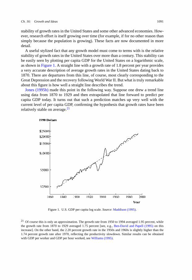
A useful stylized fact that any growth model must come to terms with is the relativestability of growth rates in the United States over more than a century. This stability canbe easily seen by plotting per capita GDP for the United States on a logarithmic scale,as shown inFigure 1. A straight line with a growth rate of 1.8 percent per year providesa very accurate description of average growth rates in the United States dating back to1870. There are departures from this line, of course, most clearly corresponding to theGreat Depression and the recovery following World War II. But what is truly remarkableabout this figure is how well a straight line describes the trend.

Jones (1995b)made this point in the following way. Suppose one drew a trend lineusing data from 1870 to 1929 and then extrapolated that line forward to predict percapita GDP today. It turns out that such a prediction matches up very well with thecurrent level of per capita GDP, confirming the hypothesis that growth rates have beenrelatively stable on average.21

Figure 1. U.S. GDP per capita log scale.Source: Maddison (1995).

21 Of course this is only an approximation. The growth rate from 1950 to 1994 averaged 1.95 percent, whilethe growth rate from 1870 to 1929 averaged 1.75 percent [see, e.g.,Ben-David and Papell (1995)on thisincrease]. On the other hand, the 2.20 percent growth rate in the 1950s and 1960s is slightly higher than the1.74 percent growth rate after 1970, reflecting the productivity slowdown. Similar results can be obtainedwith GDP per worker and GDP per hour worked, seeWilliams (1995).

1092 C.I. Jones

This stylized fact represents an important benchmark that any growth model mustmatch. Whatever the engine driving long run growth, it must (a) be able to producerelatively stable growth rates for a century or more, and (b) must not predict that growthrates in the United States over this period of time should depart from such a pattern. Tosee this force of this argument, consider first a theory likeLucas (1988)that predictsthat investment in human capital is the key to growth. In this model, the growth rate ofthe economy is proportional to the investment rate in human capital. But if investmentrates in human capital have risen significantly in the 20th century in the United States,as data on educational attainment suggests, this is a problem for the theory. It couldbe rescued if investment rates in human capital in the form of on-the-job training havefallen to offset the rise in formal education, but there is little evidence suggesting thatthis is the case.

This stylized fact is even more problematic for the first-generation idea-based growthmodels ofRomer (1990), Aghion and Howitt (1992)andGrossman and Helpman (1991)(R/AH/GH). These models predict that growth is an increasing function of researcheffort, but research effort has apparently grown tremendously over time. As one exampleof this fact, considerFigure 2. This figure plots an index of the number of scientists andengineers engaged in research in the G-5 countries. Between 1950 and 1993, this indexof research effort rose by more than a factor of eight. In part this is because of thegeneral growth in employment in these countries, but as the figure shows, it also reflectsa large increase in the fraction of employment devoted to research. A similar fact can be

Figure 2. Researchers and employment in the G-5 countries (index).Note. From calculations inJones(2002b). Data on researchers before 1950 in countries other than the United States is backcasted using the1965 research share of employment. The G-5 countries are France, Germany, Japan, the United Kingdom and

the United States.


documented using just the data for the United States, or by looking at spending on R&Drather than employment.22 The bottom line is that resources devoted to research haveexhibited a tremendous amount of growth in the post-war period, while growth rates inthe United States have been relatively stable. The implication is that models that exhibitstrong scale effects are inconsistent with the basic trends in aggregate data. Evidencelike this is one of the main arguments in favor of models that exhibit weak scale effectsinstead.23

5.2. Growth effects and policy invariance

At some level, the rejection of models with strong scale effects in favor of models withweak scale effects should not be especially interesting. The only difference between thetwo models, as discussed above, is essentially the strength of the knowledge spilloverparameter. In expanding variety models, isφ = 1 or isφ < 1? Nothing in the evidencenecessarily rules outφ = 0.95, and continuity arguments suggest that the economics ofφ = 0.95 andφ = 1 cannot be that different.

The main difference in the economic results that one obtains in the two models per-tains to the ability of changes in policy to alter the long-run growth rate of the economy.In the models that exhibit strong scale effects, the long-run growth rate is an increasingfunction of the number of researchers. Hence, a policy that increases the number of re-searchers, such as an R&D expenditure subsidy, will increase the long-run growth rate.In contrast, ifφ < 1, then the long-run growth rate depends on elasticities of produc-tion functions and on the rate of population growth. To the extent that these parametersare unaffected by policy – as one might naturally take to be the case, at least to a firstapproximation – policy changes such as a subsidy to R&D or a tax on capital will haveno affect on the long-run growth rate. They will of course affect the long-run level ofincome and will affect the growth rate along a transition path, but the long-run growthrate is invariant to standard policy changes.

This statement can be qualified in a couple of ways. First, the population growth rateis really an endogenous variable determined by fertility choices of individuals. Policychanges can affect this choice and hence can affect long-run growth even in a modelwith weak scale effects, as shown inJones (2003). However, the effects can often becounter to the usual direction. For example, a subsidy to R&D can lead people to per-form more research and have fewer kids, reducing fertility. Hence a subsidy to research

22 There are several ways to look at the R&D spending share of GDP. For total R&D expenditures as ashare of GDP in the United States, most of the increase in the R&D share occurs before 1960. However, ifone substracts out R&D expenditures on defense and space (which might be a reasonable thing to do sincegovernment output is valued at cost), or if one focuses on non-federally-financed research, the trend in the U.S.share emerges clearly; see Chapter 4 of the NSF’sScience and Engineering Indicators, 2004. Alternatively,there are substantial trends in the R&D shares for most of the other G-7 countries; in addition to the 2004edition, see also the 1993 edition of the NSF’sScience and Engineering Indicators to get data on the researchshares back to 1970.23 The other main argument is the “linearity critique” discussed further in Section6.2.

1094 C.I. Jones

can reduce the long-run growth rate. This can be true even if it is optimal to subsidizeresearch – this kind of model makes clear that long-run growth and welfare are two verydifferent concepts. The second qualification is that one can imagine subsidies that af-fect the direction of research and that can possibly affect long-run growth. For example,Cozzi (1997)constructs a model in which research can proceed in different directionsthat may involve different knowledge spillover elasticities. By shifting research to thedirections with high spillovers, it is possible to change the long-run growth rate.

Despite these qualifications, it remains true that in the semi-endogenous growth mod-els written to address the problem of strong scale effects, straightforward policies do notaffect the long-run growth rate. This has led a number of researchers to seek alternativemeans of eliminating the strong scale effects prediction while maintaining the potencyof policy to alter the long-run growth rate. Key papers in this line of research includeYoung (1998), Peretto (1998), Dinopoulos and Thompson (1998)andHowitt (1999)(Y/P/DT/H).

These papers all work in a similar way.24 In particular, each adds a second dimensionto the model, so that research can improve productivity for a particular product or canadd to the variety of products. To do this in the simplest way, suppose that aggregateconsumption (or output) is a CES composite of a variety of different products

(62)Ct =( ∫ Bt

0Y

1/θit di

)θ

, θ > 1,

whereBt represents the variety of goods that are available at datet andYit is the outputof varietyi. Assume that each varietyYi is produced using the Romer-style technologywith φ = 1 in the simple model given earlier in Section3.

The key to the model is the way in which the number of different varietiesB changesover time. To keep the model as simple as possible, assume

(63)Bt = Lβt .

That is, the number of varieties is proportional to the population raised to some powerβ.Notice that this relationship could be given microfoundations with an idea productionfunction analogous to that in Equation(16).25

Finally, let us assume each intermediate variety is used in the same quantity so thatYit = Yt , implying Ct = Bθ

t Yt . Per capita consumption is thenct = Bθt yt , and per

capita consumption growth along a balanced growth path is

(64)gc = θgB + σgA = θβn + σgA.

Assuming an idea production function withφ = 1, like that in R/AH/GH, the growthrate of the stock of ideas is proportional to research effort per variety,LAt/Bt = sLt/Bt ,

(65)gA = νsLt

Bt

= νsL1−βt .

24 This section draws heavily onJones (1999).25 For example, ifB = LBγ , then Equation(63) holds along a balanced growth path withβ = 1/(1 − γ ).


Substituting this equation back into(64) gives the growth rate of per capita output as afunction of exogenous variables and parameters

(66)gc = θβn + σνsL1−βt .

With β = 1 so thatBt = Lt , the strong scale effect is eliminated from the model,while the effect of policy on long-run growth is preserved. That is, a permanent increasein the fraction of the labor force working in research,s, will permanently raise thegrowth rate. This is the key result sought by the Y/P/DT/H models.

However, there are two important things to note about this result. First, it is very frag-ile. In particular, to the extent thatβ �= 1, problems reemerge. Ifβ < 1, then the modelonce again exhibits strong scale effects. Alternatively, ifβ > 1, then changes ins nolonger permanently affect the long-run growth rate. Thus, the Y/P/DT/H result dependscrucially on a knife-edge case for this parameter value, in addition to the Romer-likeknife-edge assumption ofφ = 1. Second, as the first term in Equation(66) indicates,the model still exhibits the weak form of scale effects. This result is not surprising giventhat these are idea-based growth models, but it is useful to recognize since many of thepapers in this literature have titles that include the phrase “growth without scale effects”.What these titles really mean is that the papers attempt to eliminate strong scale effects;all of them still possess weak scale effects. These points are discussed in more detail inJones (1999)andLi (2000, 2002).

5.3. Cross-country evidence on scale effects

One source of evidence on the empirical relevance of scale effects comes from lookingacross countries or regions at a point in time. Consider first the ideal cross-sectionalevidence. One would observe two regions, one larger than the other, that are otherwiseidentical. The two regions would not interact in any way and the only source of newideas in the two regions would be the regions’ own populations. In such an ideal ex-periment, one could search for scale effects by looking at the stock of ideas and at percapita income in each region over time. In the long-run, one would expect that the largerregion would end up being richer.

In practice, of course, this ideal experiment is never observed. Instead, we have dataon different countries and regions in the world, but these regions almost certainly shareideas and they almost certainly are not equal in other dimensions. It falls to clever econo-metricians to use this data to approximate the ideal experiment. No individual piece ofevidence is especially compelling, but the collection taken together does indeed suggestthat the cross-sectional evidence on scale effects supports the basic model.

Certainly the most creative approximation to date is found inKremer (1993)and laterappears in the Pulitzer Prize-winning bookGuns, Germs, and Steel by Diamond (1997).The most recent ice age ended about 10,000 B.C. Before that time, ocean levels werelower, allowing humans to migrate around the world – for example across the BeringStrait and into the Americas. In this sense, ideas could diffuse across regions. However,

1096 C.I. Jones

with the end of the ice age, sea levels rose, and various regions of the world were effec-tively isolated from each other, at least until the advent of large sailing ships sometimearound the year 1000 or 1500. In particular, for approximately 12,000 years, five regionswere mutually isolated from one another: the Eurasian/African continents, the Ameri-cas, Australia, Tasmania (an island off the coast of Australia), and the Flinders Island(a very small island off the coast of Tasmania). These regions are also nicely ranked interms of population sizes, from the relatively highly-populated Eurasian/African conti-nent down to the small Flinders Island, with a population that likely numbered fewerthan 500.

It is plausible that 12,000 years ago these regions all had similar technologies: allwere relatively primitive hunter-gatherer cultures. Now fast-forward to the year 1500when a wave of European exploration reintegrates the world. First, the populous OldWorld has the highest level of technological sophistication; they are the ones doing theexploring. The Americas follow next, with cities, agriculture, and the Aztec and Mayancivilizations. Australia is in the intermediate position, having developed the boomerang,the atlatl, fire-making, and sophisticated stone tools, but still consisting of a hunter-gatherer culture. Tasmania is relatively unchanged, and the population of Flinders Islandhad died out completely. The technological rank of these regions more than 10,000 yearslater matches up exactly with their initial population ranks at the end of the last ice age.

Turning to more standard evidence from the second-half of the 20th century, one isfirst struck by the apparent lack of support for the hypothesis of weak scale effects.The most populous countries of the world, China and India, are among the poorest,while some of the smallest countries like Hong Kong and Luxembourg are among therichest. And the countries with the most rapid rates of population growth – many inAfrica – are among the countries with the slowest rates of per capita income growth.However, a moment’s thought suggests that one must be careful in interpreting this evi-dence. It is clearly not the case that Hong Kong and Luxembourg are isolated countriesthat grow solely based on the ideas created by their own populations. These countriesbenefit tremendously from ideas created around the world. And in the case of the poorcountries of the world, “other things” are clearly not equal. These countries have verydifferent levels of human capital and different policies, institutions, and property rightsthat contribute to their poverty. Hence, we must turn to econometric evidence that seeksto neutralize these differences.

The clearest cross-country evidence in favor of weak scale effects comes from papersthat explicitly control for differences in international trade. Intuitively, openness to in-ternational trade is likely related to openness to idea flows, and the flow of ideas fromother countries is one of the key factors that needs to be neutralized.Backus, Kehoeand Kehoe (1992), Frankel and Romer (1999)andAlcala and Ciccone (2002)are themain examples of this line of work, and all find an important role for scale.Alcala andCiccone (2002)provide what is probably the best specification, controlling for bothtrade and institutional quality (and instrumenting for these endogenous variables), butthe results inFrankel and Romer (1999)are similar. Alcala and Ciccone find a long-run elasticity of GDP per worker with respect to the size of the workforce that is equal


to 0.20.26 That is, holding other things equal, a 10 percent increase in the size of theworkforce in the long run is associated with a 2 percent higher GDP per worker.27

Other cross-country studies, of course, have not been able to precisely estimate thiselasticity.Hall and Jones (1999), for example, found a point estimate of about 0.05,but with a standard error of 0.06.Sala-i-Martin (1997)does not find the size of thepopulation to be a robust variable in his four million permutations of cross-countrygrowth regressions. Finally, it should be recognized that this cross-country estimate ofthe scale elasticity is not necessarily an estimate of the structural parameterγ in theidea models presented earlier in Section4. One needs a theory of technology adoptionand idea flows in order to make sense of the estimates. For example, in a world whereideas flow to all places instantaneously, there would be no reason to find a scale effectin the cross-section evidence.

A final piece of evidence that is often misinterpreted as providing evidence againstthe weak scale effects prediction is the negative coefficient on population growth in across-country growth regression, such as inMankiw, Romer and Weil (1992). Recallthat the standard interpretation of these regressions is that they are estimating transitiondynamics. The negative coefficient on population growth is interpreted as capturing thedilution of the investment rate associated with the Solow model. Consider two countriesthat are identical but for different population growth rates. The country with the fasterpopulation growth rate must equip a larger number of new workers with the existingcapital–labor ratio, effectively diluting the investment rate. The result is that such aneconomy has a lower capital–output ratio in steady state, reducing output per workeralong the balanced growth path. But this same force is also at work in any growth model,including idea-based models, as was apparent above inResult 1(b). The implication isthat this cross-country evidence is not inconsistent with models in which weak scaleeffects play a role.

5.4. Growth over the very long run

Additional evidence on the potential relevance of scale effects to economic growthcomes from what at first might seem an unlikely place: the history of growth fromthousands of years ago to the present.

One of the important applications of models of economic growth in recent yearshas been to understand economic growth over this very long time period. Many of ourworkhorse models of growth were constructed with an eye toward 20th-century growth.Asking how well they explain growth over a much longer period of time therefore pro-vides a nice test of our models.

26 The standard error of this particular point estimate is about 0.10. Across different specifications, the elas-ticity ranges from a low of about 0.10 to a high of about 0.40.27 Of course in the model with trade, other things would not be equal: a change in population would almostsurely affect the trade-GDP ratios that measure openness in the regression.

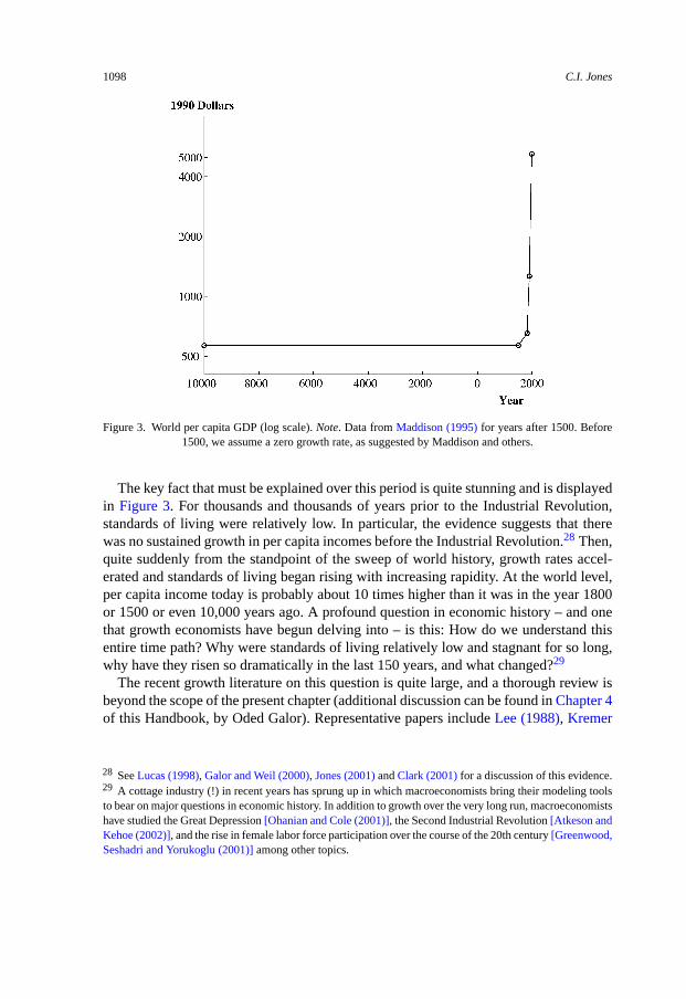
1098 C.I. Jones

Figure 3. World per capita GDP (log scale).Note. Data fromMaddison (1995)for years after 1500. Before1500, we assume a zero growth rate, as suggested by Maddison and others.

The key fact that must be explained over this period is quite stunning and is displayedin Figure 3. For thousands and thousands of years prior to the Industrial Revolution,standards of living were relatively low. In particular, the evidence suggests that therewas no sustained growth in per capita incomes before the Industrial Revolution.28 Then,quite suddenly from the standpoint of the sweep of world history, growth rates accel-erated and standards of living began rising with increasing rapidity. At the world level,per capita income today is probably about 10 times higher than it was in the year 1800or 1500 or even 10,000 years ago. A profound question in economic history – and onethat growth economists have begun delving into – is this: How do we understand thisentire time path? Why were standards of living relatively low and stagnant for so long,why have they risen so dramatically in the last 150 years, and what changed?29

The recent growth literature on this question is quite large, and a thorough review isbeyond the scope of the present chapter (additional discussion can be found inChapter 4of this Handbook, by Oded Galor). Representative papers includeLee (1988), Kremer

28 SeeLucas (1998), Galor and Weil (2000), Jones (2001)andClark (2001)for a discussion of this evidence.29 A cottage industry (!) in recent years has sprung up in which macroeconomists bring their modeling toolsto bear on major questions in economic history. In addition to growth over the very long run, macroeconomistshave studied the Great Depression[Ohanian and Cole (2001)], the Second Industrial Revolution[Atkeson andKehoe (2002)], and the rise in female labor force participation over the course of the 20th century[Greenwood,Seshadri and Yorukoglu (2001)]among other topics.

http://dx.doi.org/10.1016/S1574-0684(05)01004-X


(1993), Goodfriend and McDermott (1995), Lucas (1998), Galor and Weil (2000), Clark(2001), Jones (2001), Stokey (2001), Hansen and Prescott (2002)andTamura (2002).

In several of these papers, scale effects play a crucial role. Scale is at the heart of themodels ofLee (1988), Kremer (1993)andJones (2001), and it also plays an importantrole in getting growth started in the model based on human capital inGalor and Weil(2000).

The role of scale effects in these models can be illustrated most effectively by lookingat the elegant model ofLee (1988). The three key equations of that model are:

(67)Yt = AtL1−βt T

βt , Tt = 1,

(68)At

At

= γ logLt , A0 given,

(69)Lt

Lt

= α

(log

Yt

Lt

− log y

), L0 given.

Equation(67) describes a production function that depends on ideasA, laborL, andlandT , which is assumed to be in fixed supply and normalized to one. Equation(68)is a Romer-like production function for new ideas. Notice that we have assumed theφ = 1 case so that we can get an analytic solution below, but the nature of the resultsdoes not depend on this assumption. Notice also that we assume all labor can produceideas, and we assume a log form. This makes the model log-linear, which is the sec-ond key assumption needed to get a closed-form solution. Finally, Equation(69) is aMalthusian equation describing population growth. If output per person is greater thanthe subsistence parametery, then population grows; if less then population declines.

The model can be solved as follows. First, choose the units of output such that thesubsistence term gets normalized to zero, logy = 0. Next, leta ≡ logA and ≡ logL.Then the model reduces to a linear homogeneous system of differential equations:

(70)at = γ t ,

(71)t = αat − αβt .

It is straightforward to solve this system to find

(72)logYt

Lt

= ω1eθ1t + ω2eθ2t ,

whereθ1 > 0 andθ2 < 0 are the eigenvalues associated with this system, andω1 > 0.30

That is, the solution involves a double exponential: the natural log of output per worker

30 The differential system can be solved using linear algebra, as inBarro and Sala-i-Martin (1995, p. 480)or,even more intuitively, by writing it as a single second-order differential equation, as inBoyce and DiPrima(1997, pp. 123–125). The values for the constants in Equation(72) areθ1 = (−αβ +

√(αβ)2 + 4αγ )/2,

θ2 = (−αβ −√

(αβ)2 + 4αγ )/2, ω1 = (θ1/α)(α(a0 − β0) − θ20)/(θ1 − θ2), ω2 = (θ2/α)(θ10 −α(a0 − β0))/(θ1 − θ2).

1100 C.I. Jones

grows exponentially, so that the growth rate of output per worker,y ≡ Y/L, itself growsexponentially,

(73)yt

yt

= ω1θ1eθ1t + ω2θ2eθ2t .

Mathematically, it is this double exponential growth that allows the model to deliver agraph that looks approximately like that inFigure 3.

Analytically, Lee’s result is extremely nice. However, the analytic results are obtainedonly by simplifying the model considerably – perhaps too much. For example, the modelgenerates double exponential growth in population as well. As shown inKremer (1993),this pattern fits the broad sweep of world history, but it sharply contradicts the demo-graphic transition that has set in over the last century, where population growth rateslevel off and decline. In addition, the analytic results require the strong assumption thatφ = 1.

If one wishes to depart from the log-linear structure of Lee’s model, the analysismust be conducted numerically. This is done inJones (2001), with a more realisticdemographic setup and with an idea production function that incorporatesφ < 1. Thebasic insights fromLee (1988)apply over the broad course of history, but the modelalso predicts a demographic transition and a leveling off of per capita income growthin the 20th century. The model with weak scale effects, then, is able to match the basicfacts of income and population growth over both the very long run and the 20th century.

The economic intuition for these results is straightforward. Thousands and thousandsof years ago, the population was relatively small and the productivity of the populationat producing ideas was relatively low. Per capita consumption, then, stayed around theMalthusian level that kept population constant (y in the Lee model above). Suppose ittook 1000 years for this population to discover a new idea. With the arrival of the newidea, per capita income and fertility rose, producing a larger population. Diminishingreturns associated with a fixed supply of land drove consumption back to its subsistencelevel, but now the population was larger. Instead of requiring 1000 years to produce anew idea, this larger population produced a new idea sooner, say in 800 years. Con-tinuing along this virtuous circle, growth gradually accelerated. Provided the economicenvironment is characterized by a sufficiently large degree of increasing returns (to off-set the diminishing returns associated with limited land), the acceleration in populationgrowth produces a scale effect that leads to the acceleration of per capita income growth.Eventually, the economy becomes sufficiently rich that a demographic transition sets in,leading population growth and per capita income growth to level out.31

31 It is even possible for the demographic transition to drive population growth rates down to zero, in whichcases per capita income growth rates decline as well. There is always growth in this world – even a constantpopulation produces new ideas – but the growth rate is no longer exponential. SeeJones (2001).


5.5. Summary: scale effects

Virtually all idea-based growth models involve some kind of scale effect, for the basicreason laid out earlier in the presentation of the Idea Diagram. The strong scale effectsof many first-generation idea-based growth models – in which the growth rate of theeconomy is an increasing function of its size – are inconsistent with the relative stabilityof growth rates in the United States in the 20th century. Subsequent idea-based growthmodels replaced this strong scale effect with a weak scale effect, where the long-runlevel of per capita income is an increasing function of the size of the economy. Thelong-run growth rate in these models is generally an increasing function of the rate ofgrowth of research effort, which in turn depends on the population growth rate of thecountries contributing to world research. However, this growth rate is typically taken tobe exogenous, producing the policy-invariance results common in these models.

Simple correlations (say of income per person with population, or growth rates of percapita income with population growth rates) on first glance appear to be inconsistentwith weak scale effects. However, the ceteris paribus assumption is not valid for suchcomparisons. Attempts to render other things equal using careful econometrics certainlyreveal no inconsistency with the weak scale effects prediction, although they also do notnecessarily provide precise estimates of the magnitude of the key scale elasticity.

More broadly, the very long-run history of economic growth appears consistent withweak scale effects. Models in which scale plays an important role have proven capableof explaining the very long-run dynamics of population and per capita income, includ-ing the extraordinarily slow growth over much of history and the transition to moderneconomic growth since the Industrial Revolution.

6. Growth accounting, the linearity critique, and other contributions

This section summarizes a variety of additional insights related to idea-based growthmodels. Section6.1 discusses growth accounting in such models, showing that scaleeffects have accounted for only about 20 percent of U.S. growth in the post-war period.Increases in educational attainment and increases in R&D intensity account for the re-maining 80 percent. Section6.2considers a somewhat controversial “linearity critique”of endogenous growth models that first appeared in the 1960s. Finally, Section6.3willdiscuss briefly several other important contributions to the literature on growth and ideasthat have not yet been mentioned.

6.1. Growth accounting in idea-based models

Growth accounting in a neoclassical framework has a long, illustrious tradition, begin-ning with Solow (1957). As is well known, such accounting typically finds a residual,which is labeled “total factor productivity growth” (TFP growth). In some ways, en-dogenous growth models can be understood as trying to find ways to endogenize TFP

1102 C.I. Jones

growth, i.e. to make it something that is determined within the model rather than as-sumed to be completely exogenous. Having such a model in hand, then, it is quite naturalto ask how the model decomposes growth into its sources. That is, quantitatively, howdoes a particular model account for growth?

Jones (2002b)conducts one of these growth accounting exercises in an economicenvironment that is basically identical to that analyzed in Section4. In the long run inthat model, per capita growth is proportional to the rate of population growth of theidea-producing regions. Off a balanced growth path, of course, growth can come fromtransition dynamics, for example, due to capital deepening or to rapid growth in thestock of ideas. Given the stylized fact that U.S. growth rates have been relatively stableover a long period of time, one might be tempted to think that the U.S. is close to itsbalanced growth path so that growth due to transition dynamics is negligible. On thecontrary, however, Jones shows that just the opposite is true. Approximately 80 percentof U.S. growth in the post-war period is due to transition dynamics associated in roughlyequal parts with increases in educational attainment and with increases in world R&Dintensity. Only about 20 percent of U.S. growth is attributed to the scale effect associatedwith population growth in the idea-generating countries.32

This finding raises a couple of important questions. First, how it is that growth ratescan be relatively stable in the United States if transition dynamics are so important? Theanswer proposed byJones (2002b)can be seen in a simple analogy. Consider a standardSolow (1956)model that begins in steady state. Now suppose the investment rate in-creases permanently by 1 percentage point. We know that growth rates rise temporarilyand then decline. Now suppose the investment rate, rather than staying constant, growsexponentially. We know that this cannot happen forever since the investment rate isbounded below one. However, it could happen for awhile. In such a world, it is possiblefor the continued increases in the investment rate to sustain a constant growth rate that ishigher than the long-run growth rate. In the idea-based growth model analyzed byJones(2002b), it is not the investment rate in physical capital that is driving the transition dy-namics. Instead, educational attainment and research intensity (the fraction of the laborforce working to produce ideas in advanced countries) appear to be rising smoothly ina way that can generate stable growth, at least as an approximation.

The second natural question raised by this accounting concerns the future of U.S.growth. If 80 percent of U.S. growth is due to transition dynamics, then a straight-forward implication of the result is that growth rates could slow substantially at somepoint in the future when the U.S. transits to its balanced growth path. To the extent thatpopulation growth rates in the idea-producing countries are declining, this finding isreinforced. Still, there are many other qualifications that must be made concerning thisresult. Most importantly, it is not clear when the transition dynamics will “run out”, par-ticularly since the fraction of the labor force engaged in research seems to be relatively

32 Comin (2002)suggests that the contribution of R&D to growth could be even smaller. The key assumptionshe needs to get this result are that R&D as a share of GDP is truly small, as measured, and that the elasticityof output with respect to ideas is small.


small. In addition, the increased development of countries like China and India meansthat the pool of potential idea creators could rise for a long time.

6.2. The linearity critique

This section considers the somewhat controversial “linearity critique” of endogenousgrowth models that first appeared in the 1960s. A coarse version of the criticism is thatsuch models rely on a knife-edge assumption that a particular differential equation islinear in some sense. If the linearity is relaxed slightly, the model either does not gener-ate long-run growth or exhibits growth rates that explode. This section first presents thebasic issue and then attempts to show how it can be used productively to make progressin our understanding of economic growth.33

Growth models that are capable of producing steady-state growth require strong as-sumptions. For example, it is well known that steady-state growth is possible onlyif technological change is labor-augmenting or if the production function is Cobb–Douglas.34 Another requirement is that the model must possess a differential equationthat is linear. That is, all growth models that exhibit steady-state growth ultimately reston an assumption that some differential equation takes the form

(74)X = X.

Growth models differ primarily according to the way in which they label theX variableand the way in which they fill in the blank in this differential equation.35

For example, in theSolow (1956)model without technological progress, the differen-tial equation for capital accumulation is less than linear, and the model cannot producesustained exponential growth. On the other hand, when one adds exogenous techno-logical change in the form of a linear differential equationAt = gAt , one obtains amodel with steady-state growth. In the AK growth models ofFrankel (1962)andRebelo(1991), the law of motion for physical capital is assumed to be linear. In the human cap-ital model ofLucas (1988), it is the law of motion for human capital accumulation thatis assumed to be linear. Finally, in the first-generation idea-based growth models ofRomer (1990), Aghion and Howitt (1992)andGrossman and Helpman (1991), it is theidea production function itself that is assumed to be a linear differential equation.

This kind of knife-edge requirement has made economists uncomfortable for sometime.Stiglitz (1990)andCannon (2000)note that this is one reason endogenous growthmodels did not catch on in the 1960s even though several were developed.36 Solow(1994)resurrects this criticism in arguing against recent models of endogenous growth.

33 This section draws heavily onJones (2003).34 See, for example, the Appendix to Chapter 2 inBarro and Sala-i-Martin (1995).35 This approach to characterizing growth models is taken fromRomer (1995). Two qualifications apply.First, this linearity can be hidden in models with multiple state variables, as discussed inMulligan andSala-i-Martin (1993). Second, linearity is an asymptotic requirement, not a condition that needs to hold atevery point in time, as noted byJones and Manuelli (1990).36 The very nice AK model ofFrankel (1962)is perhaps the clearest example.

1104 C.I. Jones

What is not sufficiently well appreciated, however, is thatany model of sustainedexponential growth requires such a knife-edge condition. Neoclassical growth modelsare not immune to this criticism; they just assume the linearity to be completely unmo-tivated. One can then proceed in two possible directions. First, one can give up on thedesire that a model exhibit steady-state growth. It is not clear where this direction leads,however. One still wants a model to be able to match the steady exponential growth ex-hibited in the United States for the last 125 years, and it seems likely that a model thatproduces this kind of behavior will require a differential equation that is nearly linear.Alternatively, one can see the linearity critique as an opportunity for helping us improveour growth models. That is, if a growth model requires a linear differential equation, onecan look for an economic explanation for why linearity should hold and/or seek empir-ical evidence supporting the linearity.

To see how this might work, consider briefly the main types of endogenous growthmodels and the key differential equations of those models:

1. AK model,K = sKφ .2. Lucas model,h = uhφ .3. R/AH/GH model,A = HAAφ .4. Fertility model,N = (b − d)Nφ .

In each case, we can ask the question: “Why should we believe thatφ ≈ 1 is validin this model?”. In particular, we consider the following experiment. Suppose we holdconstant the individual decision variables (e.g. the investment rate in physical capital ortime spent accumulating human capital). Suppose we then double the state variable. Dowe double the change in the state variable?

In the AK model,φ is the elasticity of output with respect to capital. In the absence ofexternalities, this elasticity is the share of capital in income. Narrowly interpreting themodel as applying to physical capital, one gets a benchmark value of about 1/3. Somepeople prefer to include human capital as well, which can get the share a little higher.37

But then one must appeal to large externalities, and these externalities must be exactlythe right size in order to getφ ≈ 1.

Now turn to the human capital model ofLucas (1988). Consider a representativeagent who lives forever and spends 10 hours per week studying to obtain skills. Are theskills that are added by one period of this studying doubled if the individual’s stock ofhuman capital is doubled? A natural benchmark might be that studying for 10 hours aweek adds the same amount, whether one is highly skilled or has little skill. It is farfrom obvious that the 10 hours of studying increases skills proportionately over time.38

37 I personally think this is a mistake. Human capital is different from physical capital in many ways and getstreated differently in models that are careful about the distinction, e.g.Bils and Klenow (2000).38 A subtlety in thinking through the human capital model comes from the Mincerian wage regression ev-idence. Each year of schooling appears to raise a worker’s wage – and hence productivity – by a constantpercentage. One might be tempted to use this to argue thatφ = 1 in the human capital case.Bils and Klenow(2000)suggest instead that a human capital accumulation equation of the formh = eθuhφ is the right way tocapture this evidence.


This chapter has already discussed the Romer/AH/GH assumption ofφ = 1. Recallthat one can make a case forφ < 0 if it gets harder over time to find new ideas orφ > 0if knowledge spillovers increase research productivity, or evenφ = 0 if researchersproduce a constant number of ideas with each unit of effort. The case ofφ = 1 appearsto have little in the way of intuition or evidence to recommend it.

Finally, the last case above suggests placing the linearity in the equation for popula-tion growth, as was done implicitly in the models discussed earlier in the chapter. It canbe thought of in this way: Letb andd denote the birth rate and the mortality rate foran individual, respectively. Hold constant an individual’s fertility behavior, and supposewe double the number of people in the population. A natural benchmark assumption isthat we double the number of offspring. This is the intuition for why a linear differentialequation makes sense as a benchmark for the population growth equation.

More generally, I would make the claim that population growth is the least objection-able place to locate a linear differential equation in a growth model, for two reasons.First, if we take population as exogenous and feed in the observed population growthrates into an idea-based growth model, we can explain sustained exponential growth. Noadditional linearity is needed. Second, the intuition above suggests that it is not crazy tothink this differential equation might be close to linear: people reproduce in proportionto their number.39

This is one example of how the linearity critique can be used productively. Propo-nents of particular endogenous growth models can seek evidence and economic insightssupporting the hypothesis that the particular engine of growth in a model does indeedinvolve a differential equation that is close to linear.

6.3. Other contributions

There are a number of other very interesting papers that I have not had time to discuss.These should be given more attention than simply the brief mention that follows, butthis chapter is already too long.

Kortum (1997)andSegerstrom (1998)are two important papers that present growthmodels that exhibit weak scale effects. Both are motivated in part by the stylized factthat total U.S. patents granted to U.S. inventors does not show a large time trend fornearly a century, from roughly 1910 until 1990. If patents are a measure of useful ideas,this fact suggests that the number of new ideas per year might have been relatively stableduring a time when per capita income was growing at a relatively constant rate. Howcan this be? In the models provided above, the stock of ideas grows at a constant rate,just like output.Kortum (1997)andSegerstrom (1998)solve this puzzle by supposingthat ideas, at least on average, representproportional improvements in productivity. The

39 This does not mean that fertility behavior,b, will ensure a positive rate of population growth forever. Thatis a different question. Indeed,Jones (2001)supposes that a demographic transition ultimately leads to zeropopulation growth in attempting to explain growth over the very long run.

1106 C.I. Jones

papers also assume that new ideas are increasingly difficult to obtain, so that in steadystate, a growing number of researchers produce a constant number of new ideas, whichin turn leads to a constant rate of exponential growth.

Romer (1994a)makes an interesting point that appears (at least based on citations)to have been under appreciated in the literature. The paper considers the welfare cost oftrade restrictions from the standpoint of models in which ideas play an important role.In neoclassical models, trade restrictions, like other taxes, typically have small effectsassociated with Harberger triangles that depend on the square of the tax rate. In contrast,Romer shows that if trade restrictions reduce the range of goods (ideas) available withina country, the welfare affect is proportional to the level of the tax rate rather than itssquare. As a result, distortions that affect the use of ideas can have much larger welfareeffects than those same distortions in neoclassical models.

Acemoglu (2002)surveys a number of important results that come from thinkingabout the direction of technological change. In this general framework, researchers canchoose to search for ideas that augment different factors. For example, they may searchfor ideas that augment capital or skilled labor or unskilled labor. Other things equal,a market size effect suggests that research will be targeted toward augmenting factorsthat are in greater supply, especially when these factors can be easily substituted forother factors of production.

Greenwood, Hercowitz and Krusell (1997)and Whelan (2001)focus on the rapidtechnological change that is associated with the declines in the relative prices of con-sumer and producer durables (driven in large part by the rapid declines in the quality-adjusted price of semiconductors).Greenwood, Hercowitz and Krusell (1997)show thatinvestment-specific technological change can account for roughly half of per capita in-come growth in the United States in recent decades.Whelan (2001)extends this analysisby tying it to the introduction of chained indexes in the national income and product ac-counts.

Finally, it is worth mentioning again that this chapter has largely omitted a very im-portant part of the literature on growth and ideas, that associated with the Schumpeterianmodels ofAghion and Howitt (1992)andGrossman and Helpman (1991). These modelswere applied in detail to international trade inGrossman and Helpman (1991). Aghionand Howitt (1998)contain a rich analysis of an even wider range of applications, tosuch topics as unemployment, the effects of increases in competition, patent races, andleader-follower effects in R&D. In addition to these excellent treatments, a separateHandbookchapter by Aghion and Howittsurveys some of these important topics.

7. Conclusions

Thinking carefully about the way in which ideas are different from other economicgoods leads to a profound change in the way we understand economic growth. Thenonrivalry of ideas implies that increasing returns to scale is likely to characterize pro-duction possibilities. This leads to a world in which scale itself can serve as a source

http://dx.doi.org/10.1016/S1574-0684(05)01002-6


of long run growth. The more inventors we have, the more ideas we discover, and thericher we all are. This also leads to a world where the first fundamental welfare theoremno long necessarily holds. Perfectly competitive markets may not lead to the optimalallocation of resources. This means that other institutions may be needed to improvewelfare. The patent system and research universities are examples of such institutions,but there is little reason to think we have found the best institutions – after all theseinstitutions are themselves ideas.

While we have made much progress in understanding economic growth in a worldwhere ideas are important, there remain many open, interesting research questions. Thefirst is “What is the shape of the idea production function?” How do ideas get produced?The combinatorial calculations ofRomer (1993)andWeitzman (1998)are fascinatingand suggestive. The current research practice of modeling the idea production functionas a stable Cobb–Douglas combination of research and the existing stock of ideas is el-egant, but at this point we have little reason to believe that it is correct. One insight thatillustrates the incompleteness of our knowledge is that there is no reason why researchproductivity in the idea production function should be a smooth, monotonic function ofthe stock of ideas. One can easily imagine that some ideas lead to a domino-like un-raveling of phenomena that were previously mysterious, much like the general purposetechnologies ofHelpman (1998). Indeed, perhaps the decoding of the human genomeor the continued boom in information technology will lead to a large upward shift inthe production function for ideas.40 On the other hand, one can equally imagine situ-ations where research productivity unexpectedly stagnates, if not forever then at leastfor a long time. Progress in the time it takes to travel from New York to San Franciscorepresents a good example of this.

A second unresolved research question is “What is the long-run elasticity of outputper worker with respect to population?”. That is, how large are increasing returns toscale. This parameter (labeledγ in the main models of this chapter) is crucially relatedto the long-run rate of growth of the economy. Estimating it precisely would not onlyprovide confirmation of idea-based growth theory but would also help us in accountingfor the sources of economic growth.

Finally, a policy-related question: “What are better institutions and policies for en-couraging the efficient amount of research?”. There is a large, suggestive literature onsocial rates of return to research and on the extent to which firms might underinvestin research. Still, none of these individual studies is especially compelling, and moreaccurate estimates of these gaps would be valuable. To the extent that the returns toresearch do not reflect the marginal benefit to society, better institutions might improveallocations.

40 Dale Jorgenson, in his Handbook chapter, suggests that the information technology revolution may do justthis.

http://dx.doi.org/10.1016/S1574-0684(05)01010-5

1108 C.I. Jones

Acknowledgements

I am grateful to Philippe Aghion and Paul Romer for helpful comments, and to theNational Science Foundation for research support.

References

Acemoglu, D. (2002). “Directed technical change”. Review of Economic Studies 69 (4), 781–810.Aghion, P., Howitt, P. (1992). “A model of growth through creative destruction”. Econometrica 60 (2), 323–

351.Aghion, P., Howitt, P. (1998). Endogenous Growth Theory. MIT Press, Cambridge, MA.Alcala, F., Ciccone, A. (2002). “Trade and productivity”. Mimeo. Universitat Pompeu Fabra.Arrow, K.J. (1962a). “The economic implications of learning by doing”. Review of Economic Studies 29

(June), 153–173.Arrow, K.J. (1962b). “Economic welfare and the allocation of resources for invention”. In: Nelson, R.R.

(Ed.), The Rate and Direction of Inventive Activity. Princeton University Press (NBER), Princeton, NJ,pp. 609–625.

Atkeson, A.A., Kehoe, P.J. (2002). “The transition to a new economy following the second industrial revolu-tion”. NBER Working Paper 8676.

Backus, D.K., Kehoe, P.J., Kehoe, T.J. (1992). “In search of scale effects in trade and growth”. Journal ofEconomic Theory 58 (August), 377–409.

Barro, R.J., Sala-i-Martin, X. (1995). Economic Growth. McGraw-Hill, New York.Ben-David, D., Papell, D.H. (1995). “The great wars, the great crash, and steady-state growth: Some new

evidence about an old stylized fact”. Journal of Monetary Economics 36 (December), 453–475.Bils, M., Klenow, P. (2000). “Does schooling cause growth?”. American Economic Review 90 (December),

1160–1183.Boldrin, M., Levine, D.K. (2002). “Perfectly competitive innovation”. FRB of Minneapolis Staff Report 303.Boserup, E. (1965). The Conditions of Agricultural Progress. Aldine Publishing Company, Chicago, IL.Boyce, W.E., DiPrima, R.C. (1997). Elementary Differential Equations and Boundary Value Problems. Wiley,

New York.Cannon, E. (2000). “Economies of scale and constant returns to capital: A neglected early contribution to the

theory of economic growth”. American Economic Review 90 (1), 292–295.Clark, G. (2001). “The secret history of the industrial revolution”. Mimeo. University of California, Davis.Comin, D. (2002). “R&D? A small contribution to productivity growth”. Mimeo. New York University.Cozzi, G. (1997). “Exploring growth trajectories”. Journal of Economic Growth 2 (4), 385–399.David, P.A. (1993). “Knowledge, property, and the system dynamics of technological change”. Proceedings

of the World Bank Annual Conference on Development Economics, 1992, 215–248.DeLong, J.B. (2000). “Slouching Toward Utopia”. University of California, Berkeley. Online at:

http://econ161.berkeley.edu/TCEH/Slouch_Old.html.Diamond, J. (1997). Guns, Germs, and Steel. W.W. Norton and Co., New York.Dinopoulos, E., Thompson, P. (1998). “Schumpeterian growth without scale effects”. Journal of Economic

Growth 3 (4), 313–335.Dixit, A.K., Stiglitz, J.E. (1977). “Monopolistic competition and optimum product diversity”. American Eco-

nomic Review 67 (June), 297–308.Ethier, W.J. (1982). “National and international returns to scale in the modern theory of international trade”.

American Economic Review 72 (June), 389–405.Frankel, J.A., Romer, D. (1999). “Does trade cause growth?”. American Economic Review 89 (3), 379–399.Frankel, M. (1962). “The production function in allocation and growth: A synthesis”. American Economic

Review 52 (December), 995–1022.

http://econ161.berkeley.edu/TCEH/Slouch_Old.html


Galor, O., Weil, D. (2000). “Population, technology, and growth: From the Malthusian regime to the demo-graphic transition”. American Economic Review 90 (September), 806–828.

Goodfriend, M., McDermott, J. (1995). “Early development”. American Economic Review 85 (1), 116–133.Greenwood, J., Hercowitz, Z., Krusell, P. (1997). “Long-run implications of investment-specific technological

change”. American Economic Review 87 (3), 342–362.Greenwood, J., Seshadri, A., Yorukoglu, M. (2001). “Engines of liberation”. Mimeo. University of Rochester.Griliches, Z. (1998). R&D and Productivity: The Econometric Evidence. University of Chicago Press.Grossman, G.M., Helpman, E. (1991). Innovation and Growth in the Global Economy. MIT Press, Cambridge,

MA.Hall, R.E., Jones, C.I. (1999). “Why do some countries produce so much more output per worker than oth-

ers?”. Quarterly Journal of Economics 114 (1), 83–116.Hansen, G.D., Prescott, E.C. (2002). “Malthus to Solow”. American Economic Review 92 (4), 1205–1217.Helpman, E. (Ed.) (1998). General Purpose Technologies and Economic Growth. MIT Press, Cambridge,

MA.Howitt, P. (1999). “Steady endogenous growth with population and R&D inputs growing”. Journal of Political

Economy 107 (4), 715–730.Jones, C.I. (1995a). “R&D-based models of economic growth”. Journal of Political Economy 103 (4), 759–

784.Jones, C.I. (1995b). “Time series tests of endogenous growth models”. Quarterly Journal of Economics 110

(441), 495–525.Jones, C.I. (1999). “Growth: With or without scale effects?”. American Economic Association Papers and

Proceedings 89 (May), 139–144.Jones, C.I. (2001). “Was an Industrial Revolution inevitable? Economic growth over the very long run”.

Advances in Macroeconomics 1 (2). Article 1.http://www.bepress.com/bejm/advances/voll/iss2/artl.Jones, C.I. (2002a). Introduction to Economic Growth, second ed. W.W. Norton and Co., New York.Jones, C.I. (2002b). “Sources of U.S. economic growth in a world of ideas”. American Economic Re-

view 92 (1), 220–239.Jones, C.I. (2003). “Population and ideas: A theory of endogenous growth”. In: Aghion, P., Frydman, R.,

Stiglitz, J., Woodford, M. (Eds.), Knowledge Information and Expectations in Modern Macroeconomics:In Honor of Edmund S. Phelps. Princeton University Press, Princeton, NJ, pp. 498–521.

Jones, C.I., Williams, J.C. (1998). “Measuring the social return to R&D”. Quarterly Journal of Economics 113(4), 1119–1135.

Jones, L.E., Manuelli, R. (1990). “A convex model of economic growth: Theory and policy implications”.Journal of Political Economy 98 (October), 1008–1038.

Judd, K.L. (1985). “On the performance of patents”. Econometrica 53 (3), 567–585.Kortum, S.S. (1997). “Research, patenting, and technological change”. Econometrica 65 (6), 1389–1419.Kremer, M. (1993). “Population growth and technological change: One million B.C. to 1990”. Quarterly

Journal of Economics 108 (4), 681–716.Kremer, M. (1998). “Patent buyouts: A mechanism for encouraging innovation”. Quarterly Journal of Eco-

nomics 113 (November), 1137–1167.Kuznets, S. (1960). “Population change and aggregate output”. In: Demographic and Economic Change in

Developed Countries. Princeton University Press, Princeton, NJ.Lee, R.D. (1988). “Induced population growth and induced technological progress: Their interaction in the

accelerating stage”. Mathematical Population Studies 1 (3), 265–288.Li, C.-W. (2000). “Endogenous vs. semi-endogenous growth in a two-R&D-sector model”. Economic Jour-

nal 110 (462), C109–C122.Li, C.-W. (2002). “Growth and scale effects: The role of knowledge spillovers”. Economics Letters 74 (2),

177–185.Lipscomb, A.A., Bergh, A.E. (1905). The Writings of Thomas Jefferson, vol. 13. Thomas Jefferson Memorial

Association, Washington. Online athttp://press-pubs.uchicago.edu/founders/documents/al_8_8sl2.html.Lucas, R.E. (1988). “On the mechanics of economic development”. Journal of Monetary Economics 22 (1),

3–42.

http://www.bepress.com/bejm/advances/voll/iss2/artl

http://press-pubs.uchicago.edu/founders/documents/al_8_8sl2.html

1110 C.I. Jones

Lucas, R.E. (1998). “The Industrial Revolution: Past and Future”. Mimeo. University of Chicago.Maddison, A. (1995). Monitoring the World Economy 1820–1992. Organization for Economic Cooperation

and Development, Paris.Mankiw, N.G., Romer, D., Weil, D. (1992). “A contribution to the empirics of economic growth”. Quarterly

Journal of Economics 107 (2), 407–438.Mulligan, C.B., Sala-i-Martin, X. (1993). “Transitional dynamics in two-sector models of endogenous

growth”. Quarterly Journal of Economics 108 (3), 739–774.Nordhaus, W.D. (1969). “An economic theory of technological change”. American Economic Association

Papers and Proceedings 59 (May), 18–28.Nordhaus, W.D. (2003). “The health of nations: The contribution of improved health to living standards”. In:

Murphy, K.M., Topel, R. (Eds.), Measuring the Gains from Medical Research: An Economic Approach.University of Chicago Press, Chicago, IL, pp. 9–40.

Ohanian, L., Cole, H. (2001). “Re-examining the contribution of money and banking shocks to the U.S. greatdepression”. NBER Macroeconomics Annual 16, 183–227.

Peretto, P. (1998). “Technological change and population growth”. Journal of Economic Growth 3 (4), 283–311.

Phelps, E.S. (1966). “Models of technical progress and the golden rule of research”. Review of EconomicStudies 33 (2), 133–145.

Phelps, E.S. (1968). “Population increase”. Canadian Journal of Economics 1 (3), 497–518.Quah, D.T. (1996). “The Invisible Hand and the Weightless Economy”. Mimeo. LSE Economics Department.

April.Quah, D. (2002). “Almost efficient innovation by pricing ideas”. Mimeo. LSE. June.Rebelo, S. (1991). “Long-run policy analysis and long-run growth”. Journal of Political Economy 99 (June),

500–521.Rivera-Batiz, L.A., Romer, P.M. (1991). “Economic integration and endogenous growth”. Quarterly Journal

of Economics 106 (May), 531–555.Romer, P.M. (1986). “Increasing returns and long-run growth”. Journal of Political Economy 94 (October),

1002–1037.Romer, P.M. (1987). “Growth based on increasing returns to specialization”. American Economic Review

Papers and Proceedings 77 (May), 56–62.Romer, P.M. (1990). “Endogenous technological change”. Journal of Political Economy 98 (5), S71–S102.Romer, P.M. (1993). “Two strategies for economic development: Using ideas and producing ideas”. Proceed-

ings of the World Bank Annual Conference on Development Economics 1992, 63–115.Romer, P.M. (1994a). “New goods, old theory, and the welfare costs of trade restrictions”. Journal of Devel-

opment Economics 43, 5–38.Romer, P.M. (1994b). “The origins of endogenous growth”. Journal of Economic Perspectives 8, 3–22.Romer, P.M. (1995). “Comment on a paper by T.N. Srinivasan”. In: Growth Theories in Light of the East

Asian Experience. University of Chicago Press, Chicago, IL.Romer, P.M. (2000). “Should the government subsidize supply or demand in the market for scientists and

engineers?”. NBER Working Paper 7723, June.Sala-i-Martin, X. (1997). “I just ran four million regressions”. NBER Working Paper 6252.Segerstrom, P. (1998). “Endogenous growth without scale effects”. American Economic Review 88 (5), 1290–

1310.Segerstrom, P.S., Anant, T.C.A., Dinopoulos, E. (1990). “A Schumpeterian model of the product life cycle”.

American Economic Review 80 (5), 1077–1091.Shell, K. (1966). “Toward a theory of inventive activity and capital accumulation”. American Economic As-

sociation Papers and Proceedings 56, 62–68.Sheshinski, E. (1967). “Optimal accumulation with learning by doing”. In: Shell, K. (Ed.), Essays on the

Theory of Economic Growth. MIT Press, Cambridge, MA, pp. 31–52.Simon, J.L. (1986). Theory of Population and Economic Growth. Blackwell, New York.Simon, J.L. (1998). The Ultimate Resource 2. Princeton University Press, Princeton, NJ.


Solow, R.M. (1956). “A contribution to the theory of economic growth”. Quarterly Journal of Eco-nomics 70 (1), 65–94.

Solow, R.M. (1957). “Technical change and the aggregate production function”. Review of Economics andStatistics 39 (3), 312–320.

Solow, R.M. (1994). “Perspectives on growth theory”. Journal of Economic Perspectives 8 (1), 45–54.Spence, M. (1976). “Product selection, fixed costs, and monopolistic competition”. Review of Economic

Studies 43 (2), 217–235.Stiglitz, J.E. (1990). “Comments: Some retrospective views on growth theory”. In: Diamond, P. (Ed.),

Growth/Productivity/Unemployment: Essays to Celebrate Robert Solow’s Birthday. MIT Press, Cam-bridge, MA, pp. 50–69.

Stokey, N.L. (2001). “A quantitative model of the British industrial revolution, 1780–1850”. CarnegieRochester Conference Series on Public Policy 55, 55–109.

Tamura, R. (2002). “Human capital and the switch from agriculture to industry”. Journal of Economic Dy-namics and Control 27, 207–242.

Weitzman, M.L. (1976). “On the welfare significance of national product in a dynamic economy”. QuarterlyJournal of Economics 90 (1), 156–162.

Weitzman, M.L. (1998). “Recombinant growth”. Quarterly Journal of Economics 113 (May), 331–360.Whelan, K. (2001). “Balance growth revisited: A two-sector model of economic growth”. Mimeo. Federal

Reserve Board of Governors.Williams, J.C. (1995). “Tax and Technology Policy in an Endogenous Growth Model”. Ph.D. Dissertation.

Stanford University.Young, A. (1998). “Growth without scale effects”. Journal of Political Economy 106 (1), 41–63.

Documents

GROWTH AND IDEAS - Stanford Universityweb.stanford.edu/~chadj/JonesHandbook2005.pdf · GROWTH AND IDEAS CHARLES I. JONES Department of Economics, ... creasing returns to scale, an