Growth- and Bioenergetic Models and their Application in Aquaculture of

Perch (Perca fluviatilis)

Åsa Strand

Vattenbruksinstitutionen Rapport 42 Umeå 2005

Growth- and Bioenergetic Models and their Application in Aquaculture of Perch (Perca fluviatilis)

Av Åsa Strand Vattenbruksinstitutionen, SLU, 901 83 Umeå. Introduktionsuppsats Denna rapport utgör en del av doktorandutbildningen. Målsättning med introduktionsuppsatsen är att i ett tidigt skede av doktorandutbildningen ge doktoranden en god överblick över litteraturen inom ämnesområdet. Introduktionsuppsatsen skall innehålla en kritisk granskning av kunskapen inom ämnesområdet och eventuella kunskapsluckor skall identifieras. Introductory essay This report constitutes one part of the PhD exam. The aim of the introductory essay is to give the PhD student, at the beginning of the graduate studies, a good overview of the literature in his/her research field. The essay should give a critical evaluation and identify gaps in the present knowledge. © SLU Vattenbruksinstitutionen 901 83 Umeå Tel. 090 – 786 84 43 Fax. 090 – 12 37 29 E-post. vabr@slu.se Hemsida. http://www.vabr.slu.se/ Rapport nr 42, 2005. ISSN 1101-6620 ISRN SLU-VBI-R--42--SE Tryckt av Reprocentralen SLU, Umeå.

1

CONTENTS

1. INTRODUCTION................................................................................ 2

2. ENERGY REQUIREMENT AND GROWTH MODELS .............. 4

2.1 BACKGROUND ..................................................................................... 4 2.2 BIOENERGETIC MODELS....................................................................... 4

2.2.1 The energy budget ....................................................................... 4 2.2.2 Measuring the different parts of the energy budget.................... 8 2.2.3 Pros and cons with bioenergetic models.................................... 19 2.2.4 A simplified energy budget ....................................................... 20

2.3 GROWTH MODELS.............................................................................. 23 2.3.1 Specific growth rate (SGR) ....................................................... 24 2.3.2 Daily growth coefficient (DGC)................................................ 25 2.3.3 Thermal unit growth coefficient (TGC) .................................... 26 2.3.4 Pros and cons with growth models ........................................... 28

3. FACTORS AFFECTING GROWTH AND ENERGY REQUIREMENTS .................................................................................. 31

3.1 TEMPERATURE .................................................................................. 31 3.1.1 Growth and feed intake ............................................................. 31 3.1.2 Temperature and growth modelling.......................................... 35

3.2 SEASON AND LATITUDE..................................................................... 36 3.3 PHOTOPERIOD AND ENDOGENOUS CLOCK.......................................... 37 3.4 WATER CHEMISTRY........................................................................... 38 3.5 BIOTIC FACTORS................................................................................ 39

3.5.1 Group dynamics and social interactions................................... 39 3.5.2 Stress ......................................................................................... 41 3.5.3 Living conditions ...................................................................... 42 3.5.4 Feed management...................................................................... 43

4. APPLICATIONS OF GROWTH MODELS WITH REFERENCE TO PERCH............................................................................................... 44

4.1 FEED MANAGEMENT.......................................................................... 44 4.1.1 Feed conversion model .............................................................. 44 4.1.2 Feed budget model ..................................................................... 45

REFERENCES ......................................................................................... 50

2

1. INTRODUCTION The growth of fish is a complex process which represents the net

outcome of a series of behavioral and physiological processes beginning with food intake and terminating in the deposition of animal tissue (Brett & Groves, 1979). In every commercial aquaculture situation, knowledge about actual fish growth rates, feed intake and growth efficiency in different conditions, as well as means for estimating and predicting growth, is essential for the viability of the enterprise.

The best way to maximize growth efficiency and improve farm

economy might be the use of mathematical models for growth rates and feed requirement. These models could, if used properly, be very useful tools from both a production planning and management point of view, and could aid in comparing the actual state of the farming facility with what could be biological achievable (Iwama & Tautz, 1981; Springborn et al., 1994; Cho & Bureau, 1998; Bureau et al., 2000).

However, despite many attempts to develop mathematical

expressions for describing fish growth, there exists a large diversity of approaches and concepts. It is common to find growth expressed as centimeters per month, instantaneous growth rates, percentage of change in length or percentage of change in weight, often with no reference to temperatures, feed ration or culture conditions (Iwama & Tautz, 1981).

A proper growth model will allow estimations of the fish energy

(feed) requirements and of fish growth rates. This information will allow a farmer to solve several growth related problems that arise in routine fish culture. For example predicting the final average weight of the fish after a defined rearing time, estimating the time required to achieve a given market size of the fish when rearing the fish at a defined temperature, or decide which average temperature is needed to produce a certain size of fish in a defined period of time. A good model can also provide information about stock biomass and its daily feed requirement (Iwama & Tautz, 1981; Bureau et al., 2000).

The objective of this essay is to summarize available information of

bioenergetic and growth models. The basics of bioenergetic models, as well as measurement techniques for different parts of the energy budget, will be presented. Pros and cons with energy budgets will be discussed

3

and an alternative and more simple form of the energy budget will be presented. The essay also covers different growth models and their usefulness in aquaculture. Moreover, factors affecting growth and feed intake will be considered. In the end of the essay, practical examples of the use of growth and energy requirement budgets will be demonstrated.

4

2. ENERGY REQUIREMENT AND GROWTH MODELS 2.1 Background

According to Cho (1982), the principles of bioenergetics were applied to fish already in 1914 by Ege and Krogh (1914) and several years later by Ivlev (1939). Many studies on energy utilization and expenditure have been conducted since then for several fish species (Spoor, 1946; Brett, 1962; Warren & Davis, 1967; Niimi & Beamish, 1974; Cho et al., 1976; Cho & Kaushik, 1985; Kaushik & Médale, 1994). The first bioenergetic model for fish was however not developed until 1974 by Kitchell et al. (Cui & Xie, 2000), and was originally used to simulate growth of the bluegill (Lepomis macrochirus). Models based on similar principles had been proposed earlier by other researchers (Ursin, 1967; Kerr, 1971), but the model developed by Kitchell et al., (1974), is probably the most influential and serves as a standard for later bioenergetic modeling in fish (Cui & Xie, 2000). The model has been applied to several different species, for example the three-spined stickleback (Gasterosteus aculeatus) (Allen & Wootton, 1982), the black rockfish (Sebastes melanops) (Boehlert & Yoklavich, 1983), perch (Perca fluviatilis) (Solomon & Brafield, 1972) and for the European minnow (Phoxinus phoxinus) (Cui & Wootton, 1989; Cui & Xie, 2000). In fish ecology, bioenergetic models have primarily been used to calculate food consumption from temperature and growth data (Kitchell & Breck, 1980; Rice et al., 1983; Raat, 1990), and in aquaculture, bioenergetic models have mainly been used for developing optimal feeding strategies for fish (Brett, 1979).

2.2 Bioenergetic models

2.2.1 The energy budget Since biological systems conform to the laws of thermodynamics

(Kitchell et al., 1977; Ricker, 1979; Jobling, 1985), the most simple form of a bioenergetic model can be derived from the basics of bioenergetics: “any change in body weight results from the difference between what enters the body and what leaves it” (Jobling, 1994; Jobling, 1997), and is expressed as:

)()()( PEOutEInE += (Equation 1)

5

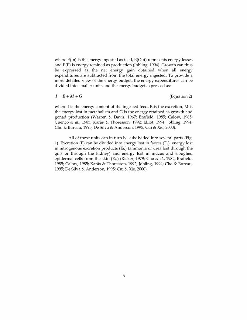
where E(In) is the energy ingested as feed, E(Out) represents energy losses and E(P) is energy retained as production (Jobling, 1994). Growth can thus be expressed as the net energy gain obtained when all energy expenditures are subtracted from the total energy ingested. To provide a more detailed view of the energy budget, the energy expenditures can be divided into smaller units and the energy budget expressed as:

GMEI ++= (Equation 2) where I is the energy content of the ingested feed, E is the excretion, M is the energy lost in metabolism and G is the energy retained as growth and gonad production (Warren & Davis, 1967; Brafield, 1985; Calow, 1985; Cuenco et al., 1985; Karås & Thoresson, 1992; Elliot, 1994; Jobling, 1994; Cho & Bureau, 1995; De Silva & Anderson, 1995; Cui & Xie, 2000).

All of these units can in turn be subdivided into several parts (Fig. 1). Excretion (E) can be divided into energy lost in faeces (EF), energy lost in nitrogenous excretion products (EN) (ammonia or urea lost through the gills or through the kidney) and energy lost in mucus and sloughed epidermal cells from the skin (EM) (Ricker, 1979; Cho et al., 1982; Brafield, 1985; Calow, 1985; Karås & Thoresson, 1992; Jobling, 1994; Cho & Bureau, 1995; De Silva & Anderson, 1995; Cui & Xie, 2000).

6

Metabolism (M) in turn can be split into metabolism related to

basic bodily functions (standard metabolism1: MS), metabolism when the fish is at rest (routine metabolism: MR), metabolism connected to activity (swimming, feeding etc.: MA) and metabolic costs associated with feed 1 The basal metabolic rate (the rate of metabolism measured under conditions of minimum environmental and physiological stress and after fasting has haltered digestive and absorptive processes) can not be used in poikilotherms as their body temperature fluctuates with the ambient temperature, and the basal metabolic rate is affected by temperature. For that reason, the standard metabolic rate for fish is defined as an animals resting and fasting metabolism at a given body temperature or in a thermoneutral environment (Cho et al., 1982; Eckert, 1988; De Silva & Anderson, 1995).

Fig. 1 Energy flow in fish. Arrows indicate the direction of energetic transfer. I, E, M and G make up the energy balance indicated by the equation I=E+M+G, where I is the ingested feed, E is the excretion, M is the metabolism and G is growth. EF, EN & EM represents the subdivisions of excretion, MF, MS, MR & MA represents the subdivisions of metabolism and GS & GR represents the subdivisions of growth. Modified from Bailey, 2003.

7

processing (MF) (Ricker, 1979; Cho et al., 1982; Calow, 1985; Elliot, 1994; Jobling, 1994). The standard metabolism is the minimum rate of energy expenditure needed to keep the animal alive (cellular activity, respiration and blood circulation). Physical activity will increase the metabolic rate due to work done against internal and external frictional forces (Cho et al., 1982; De Silva & Anderson, 1995). The greatest energy demand for most animals actually derives from activities, such as locomotion, feeding, aggression, migration and spawning (Ricker, 1979). The ingestion of feed also increases the animals’ metabolic rate, which in turn causes an increase in the animals’ temperature. This increase in metabolism is therefore termed the heat increment of feeding (Cho et al., 1982; De Silva & Anderson, 1995). The processes causing the heat increment of feeding are ingestion, digestion and absorption of feed, transformation and interconvension of the ingested substances and their retention in tissues and formation and excretion of metabolic wastes. The main biochemical basis for the heat increment is the energy required for the ingested amino nitrogen to be deaminated and excreted. However, the energy expenditures associated with heat increment of feeding is very small compared to that originating from activity (Cho et al., 1982).

In a similar manner growth (G) can be subdivided into gamete production (GG) and somatic growth (including energy storage) (GS) (Ricker, 1979; Calow, 1985; Jobling, 1994).

When all components of the basic energy budget are subdivided and substituted into equation 2, the classical bioenergetics model will look like this:

)()()( RSFARSMNF GGMMMMEEEI ++++++++= (Equation 3)

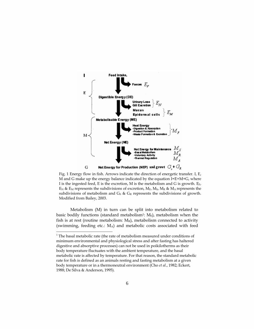
In 1979, Brett summarized 15 different energy budgets for carnivorous fish developed by different researchers. This resulted in a mean energy budget (with 95 % confidence limits) describing the relative importance of the different parts of the energy budget (Brett & Groves, 1979). As demonstrated, most energy for carnivorous fish is lost in metabolism (Equation 4, Fig. 2).

GMEI )629()744()327(100 ±+±+±= (Equation 4)

8

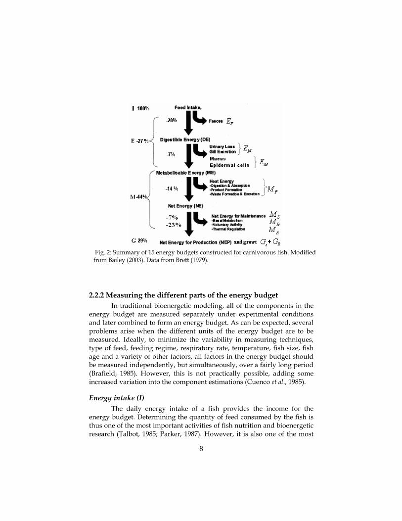
2.2.2 Measuring the different parts of the energy budget In traditional bioenergetic modeling, all of the components in the

energy budget are measured separately under experimental conditions and later combined to form an energy budget. As can be expected, several problems arise when the different units of the energy budget are to be measured. Ideally, to minimize the variability in measuring techniques, type of feed, feeding regime, respiratory rate, temperature, fish size, fish age and a variety of other factors, all factors in the energy budget should be measured independently, but simultaneously, over a fairly long period (Brafield, 1985). However, this is not practically possible, adding some increased variation into the component estimations (Cuenco et al., 1985).

Energy intake (I) The daily energy intake of a fish provides the income for the

energy budget. Determining the quantity of feed consumed by the fish is thus one of the most important activities of fish nutrition and bioenergetic research (Talbot, 1985; Parker, 1987). However, it is also one of the most

Fig. 2: Summary of 15 energy budgets constructed for carnivorous fish. Modified from Bailey (2003). Data from Brett (1979).

9

difficult factors to measure. In most cases, the energy value of a feed is less than that indicated by chemical analysis, as a part of the nutrients may be unavailable to the fish through incomplete digestion or absorption (Cho et al., 1982; Parker, 1987). Digestibility gives a relative measure of the extent to which ingested feed and its nutrient components have been digested and absorbed by the animal. Generally, fish meal is digested efficiently, often exceeding 90 %, while the apparent digestibility of various plant products (containing high levels of starch) is extremely variable and are very poorly digested by carnivorous fish (Cho et al., 1982; Cho & Bureau, 1995; De Silva & Anderson, 1995). The digestible energy (DE) value is basically the difference between the gross energy of the feed and the gross energy of the faeces derived from a known amount of feed (Fig. 1). For a well digested feed, the digestible value should approach the gross energy value of the feed (Cho et al., 1982). Digestibility is thus a useful measure of the energy potentially available for metabolism and growth from energy consumed (Knights, 1985).

It is generally assumed that all digested energy is absorbed by the fish (De Silva & Anderson, 1995), but as the catabolism of amino acids yields ammonia which is excreted by the fish, the energy available to the fish is reduced even further. The digestible energy of a diet thus often overestimates the actual energy value of the feed for the fish. However, determinations of the metabolizable energy (ME) values of feed for fish are technically difficult because of the need to quantitative both gill and urinary losses (Fig. 1) (Cho et al., 1982).

The quantity of feed ingested and the physiology of feeding and digestion can be investigated by several different methods: Observing feed intake/collect uneaten feed

The amount of feed consumed in a specific meal over a period of time can be measured directly. This can be done by manually observing actual feed intake in fish (Talbot, 1985), or by the aid of video recording (Jobling et al., 2001). However, there are many problems in observing individual feeding. Only a small number of fish can be observed simultaneously, and if feed is dispended by hand, the fish may be disturbed or stressed, and their feed consumption affected. An alternative is to compare the difference between the amounts of feed offered to the fish with the feed that has not been eaten (Talbot, 1985; De Silva & Anderson, 1995). The biggest problem with this method is to avoid

10

leakage of nutrients from the uneaten feed to the surrounding water and to separate uneaten feed from faeces (Cho et al., 1982; Brafield, 1985; Knights, 1985; Cho & Bureau, 1995; De Silva & Anderson, 1995). These methods are rather reliable and accurate, but they do not allow measurements of feed evacuation rates (Talbot, 1985). Stomach content analysis

Stomach content analysis is primarily used for qualitative estimation of dietary composition and may be carried out on either live or dead fish (Jobling et al., 2001). A population of fish is first starved to ensure that their guts are empty, after which the fish are fed to satiation and then killed at defined time intervals to see the progress of feed handling in the gut (Talbot, 1985). When using live fish, the stomach content may be removed by stomach pumping or flushing, the fish can also be induced to vomit (Jobling et al., 2001). However, theses methods are very stressful for the fish. Stomach content analysis on dead fish is very wasteful of fish, and the method is not suitable for very small fish. Data is also collected from different individuals at different time intervals, and the passage of feed through the gut can thus not be followed on an individual level (Talbot, 1985). Markers

Various indigestible chemical markers can be added to fish feeds for the study of feed intake, digestion and gastrointestinal transit rates, and both qualitative and quantitative information can be obtained (De Silva & Anderson, 1995). Examples of chemical markers are stable and unstable isotopes. The most frequently used stable isotopes are carbon-13, nitrogen-15 and sulphur-33, 34, 36 (Jardine et al., 2003). The most common unstable (radioactive) isotopes used are iodine-131 and chromium-51 (Storebacken et al., 1981). The methods of isotope use are based on measurements of the ratios of stable isotopes in the organism (Schlechtriem et al., 2004) or measuring decay (radioactivity) from unstable isotopes (Storebacken et al., 1981). Isotopes are frequently used for studying ecological processes in fish (trophic positions, mechanisms of pollutant bioaccumulation, identification of origin, stock and migrations) (Dufour & Gerdeaux, 2001), as well as determining feed intake and metabolic processes (Storebacken et al., 1981). The use of radioactive isotopes may be hazardous and subjected to many regulations and restrictions, while stable isotope techniques are clean and non-hazardous (Schlechtriem et al., 2004). The main advantage with isotope techniques is

11

that fish can be measured without killing the fish (Storebakken & Austreng, 1988).

Feed intake, as well as digestibility of the feed, can also be

estimated on an individual basis from the use of other chemical markers. If two different markers are used, feed intake and digestibility of the feed can be estimated simultaneously. One internal marker is mixed in all of the feed and one external marker is added only to a small portion of the feed. The fish are first fed with a small, but known, amount of feed marked with both the external and internal marker. The same amount must be fed each day and it is vital that all the feed is consumed. The fish are then fed the feed containing the internal marker in accordance with usual feeding practise. At the end of each daily feeding, faecal collection is started. The internal marker will concentrate relative to the digestible material in the faeces, and the relative quantities provide a measure of the extent of digestibility of the diet (Jobling et al., 2001). The advantage of this method is that fish are not starved or killed during the experiment. However, as with all marker techniques, it is crucial that the features of the marker are well known. The marker will have to be indigestible, should not influence the physiology of digestion, should move along the gut at the same rate as the rest of the feed material and should not be toxic (De Silva & Anderson, 1995). X-radiography

X-radiography is based on providing the fish with feed containing particulate X-ray-dense markers. The amount of marker eaten is measured by X-raying the fish and counting the numbers of marker particles present in the gastrointestinal tract. Standard curves for food-marker relationships are prepared by X-raying known weights of the labeled feed and counting the numbers of markers present. The amount of feed eaten by the fish is then calculated from the numbers of marker particles in the gastrointestinal tract by reference to the standard curve (Jobling et al., 2001). The advantage with this method is that fish need not be killed and can be monitored several times (although the process can be stressful) and don’t need to be starved before or after the labeled meal is offered. The main disadvantage of the method is that feed intake is measured indirectly and depends on the knowledge of the dynamics of marker flow under different physiological conditions (Talbot, 1985). Moreover, feed intake can not be measured continuously.

12

Excretion (E) Faeces

The energy which is left in faecal material is lost to the animal and is referred to as the faecal energy loss (Cho & Bureau, 1995). It can be difficult to separate faeces from the water and to avoid contamination of the faeces by uneaten feed (Knights, 1985; Cho & Bureau, 1995). One general recommendation is to collect the faeces as soon as possible after defecation as there is always some danger of overestimating digestibility and underestimate faecal energy because of leaching and dissolving of material from the faeces to the surrounding water (Brafield, 1985; Cho & Bureau, 1995; De Silva & Anderson, 1995; Jobling et al., 2001). Little can be done about faecal material voided in already solute form (Brafield, 1985). Besides undigested feed material, the faeces also contain mucosal cells, digestive enzymes and other secretions arising from metabolic activities (metabolic residues). The metabolic residues can be measured in fasting fish, and is considered to be of little significance for animals receiving normal amounts of feed (Cho et al., 1982; Cho & Bureau, 1995; De Silva & Anderson, 1995). Energy losses in waste products are not a constant proportion of the daily energy intake but vary with fish size, water temperature, and the level of energy intake (Elliot, 1994). Ammonia

Besides faeces, ammonia is the main excretory product of fish (Brafield, 1985). Most of the nitrogenous losses in catabolism of amino acids consist of excretion of ammonia through the gills (about 95%), and a much lesser part through the kidneys as ammonia and urea (Cho & Bureau, 1995). In fish, conversion of ammonia to urea is unusual and the energy lost in urea production is thus generally negligible (De Silva & Anderson, 1995). According to Brett (1979), an erroneous assumption by Winberg (1956) that the energy value of ammonia production was negligible, has contributed to overestimations of the metabolizable energy in the past (Ricker, 1979). Nitrogenous excretion is generally the smallest part of the energy budget, but the amount of energy lost is still significant, and it must be taken into account when a complete energy budget is constructed (Brafield, 1985).

The rate at which fish excretes ammonia is affected by many factors such as dietary protein quantity and quality (Brafield, 1985), and the measurements of these non-faecal losses causes both practical and technical difficulties (Cho & Bureau, 1995). When nitrogen excretion is

13

measured by respiromitry2, the flow through in the respirometer has sometimes to be stopped for several hours to allow build up of detectable ammonia levels. This can cause oxygen deficiency for the fish, which could be avoided by aeration, but with the risk of some ammonia escaping. Moreover, the ammonia may build up to levels that harm the fish. As an alternative, nitrogenous excretion can be calculated from oxygen consumption by a conversion factor based on knowledge on protein respiration and ammonia formation (Brafield, 1985).

Metabolism (M) As mentioned earlier, energy losses due to metabolic demands

usually constitute a large portion of the energy budget of a fish (Jobling, 1994). The metabolic rate of an animal will obviously vary with internal and external factors such as tissue growth and repair, chemical-, osmotic-, electrical- and mechanical internal work, locomotion, communication (Eckert, 1988) and temperature (Jobling, 1994; Brett, 1995; De Silva & Anderson, 1995; Jobling, 1997; Cui & Xie, 2000). Measurements of energy expended on metabolism have therefore caused more difficulty than any other component in the energy budget (Brafield, 1985).

Standard metabolism (MS) is often not measured as laboratory fish are rarely in that state (Brafield, 1985). Ms is also affected by the previous nutritional history of the animal, and is therefore very hard to measure accurately (Eckert, 1988; Jobling, 1994). However, it can be estimated by establishing a relationship between swimming speed and the metabolic rate in a respirometer (by measuring consumed oxygen) and then extrapolate that relationship to zero activity (Cho et al., 1982; Eckert, 1988; Jobling, 1994; Cho & Bureau, 1995). Ms can also be estimated from fasting fish (Cho & Bureau, 1995).

More commonly, the fish studied is being fed at intervals and can swim freely in the respirometer. Such activity where the fish is swimming freely but is protected from disturbances represents the normal (routine)

2A respirometer is a closed tank where a substance (for example oxygen, carbon dioxide or ammonia) is measured continuously in both the inflowing and out flowing water and recorded. As the concentrations of the substance in the inflowing and out flowing water, and the flow through the system are known, the consumption or excretion of the substance caused by the fish can be calculated (Solomon & Brafield, 1972; Cho et al., 1982; Eckert, 1988). .

14

activity (MR) of the fish (Brafield, 1985; Jobling, 1994). Fish held in respirometers may, however, show a generally lower level of activity than would be the case in nature where feed must be searched for and predators avoided. Thus, fish in respirometers may spend less energy in activity, and a larger amount on growth (Brafield 1985), once again producing erroneous estimates of the components of the energy budget. Alternatively, the fish may be stressed by the artificial environment and may have higher energy expenditures than normal. The swimming activity (MA), however, is relatively easy to measure by exposing the fish to a current, thus forcing it to swim at different speeds (Brafield, 1985; Jobling, 1994). Calorimetry

The nutritional components of the feed, which make a significant contribution to the energy supply of an animal, can be classified into three groups: carbohydrates, fats and proteins (Cho et al., 1982). Catabolism of these substances requires oxygen and results in the production of carbon dioxide, water and heat (Winberg, 1971; Ricker, 1979). The stoichometry of the oxidation of these substances thus allows calculation of the energy released as heat from measurements of respiratory exchange (Cho et al., 1982). There are three main approaches to estimate metabolism; indirect calorimetry based on measurement of oxygen consumption, indirect calorimetry from oxygen, carbon dioxide and ammonia measurements, and direct calorimetry which is based on measurements of heat increase (Brafield, 1985; Jobling, 1994; Cho & Bureau, 1995). Indirect calorimetry

Oxygen consumption and the method of indirect calorimetry can be used to quantify the metabolic energy demands (Ricker, 1979; Brafield, 1985). In this method, the total amount of oxygen consumed over a defined period is measured and multiplied by an energy conversion factor3 to produce an estimate of the energy lost (Brafield, 1985). From the stochiometry of nutrient catabolism and oxygen consumption it is estimated that the consumption of 1 g of oxygen is associated with release 3 The conversion factor is determined using information about the amounts of oxygen consumed and the amounts carbon dioxide and heat released when each of the substances (carbohydrates, fat, protein) are combusted in a bomb calorimeter (Jobling, 1994).

15

of 13,56 kJ energy (Cho et al., 1982; De Silva & Anderson, 1995). One of the prerequisites for the conversion factor to be accurate is that metabolism is aerobe. This can cause problems when estimating activity metabolism for swimming fish, since the level of anaerobic metabolism increases as fish swim (Eckert 1988; Jobling 1994). Values of the energy conversion factor also varies with the substance being respired as carbohydrates, fat and protein require different amounts of oxygen and yield different amounts of energy when metabolized (Winberg, 1971; Brafield, 1985; Eckert, 1988; Jobling, 1994). Since fish generally metabolize a mixture of substances, a new value for the energy conversion factor should be calculated at each experiment. However, most often some generally accepted coefficient is used, based on the assumption that the substances are being respired in the proportions in which they occurred in the feed, an assumption which is highly unlikely. Even though proportions of substances remaining can be measured from faeces, it is dangerous to assume that one knows the proportions in which they are really respired (Brafield, 1985).

This problem is overcome by indirect calorimetry where oxygen consumption, carbon dioxide production and ammonia build up are measured (Cho et al., 1982; Brafield, 1985; Eckert, 1988; Cho & Bureau, 1995). The measurement of both oxygen consumption and carbon dioxide production allows the calculation of the respiratory quotient (carbon dioxide produced/oxygen consumed) and from this, the relative proportion of carbohydrate and fat being oxidized can be calculated (as the respiratory quotients of carbohydrate and fat are characteristically 1,0 and 0,7, respectively) (Cho et al., 1982). The main problem with this method is that a considerable amount of carbon dioxide is present naturally in water, making the relatively small release by the fish hard to measure (Brafield, 1985). Direct calorimetry

Another method, direct calirometry, measures the quantity of heat liberated to the surroundings during the complete oxidation of organic matter (Winberg, 1971). The heat can be produced through metabolism when organic matter is oxidized by an animal or by combustion (oxidation) of a substance (Ricker, 1979; Brafield, 1985). All the chemical energy released by an animal through metabolic functions appears finally as heat. The metabolic rate of an organism can therefore be estimated by measuring the amount of energy released as heat over a given period. Such measurements are made in a calorimeter. The animal is placed in a

16

well insulated chamber and the heat lost by the animal is determined from the rise in temperature of a known mass of water used to trap the heat. A disadvantage of direct calorimetry is that the behaviour of the animal is unavoidably altered by the restrictions imposed by the measurement conditions (Eckert, 1988).

When energy content of a substance is estimated, for example when the energy content of a certain feed is analyzed, an instrument called a bomb calorimeter is used. The method is based on the combustion of a dried sample of the substance in the presence of oxygen and under high pressure, inside a “bomb” which is immersed in a known volume of water. The quantity of energy liberated during the combustion is determined from the increase in water temperature (Winberg, 1971; Cho et al., 1982; Eckert, 1988; De Silva & Anderson, 1995). Under these conditions the carbon and hydrogen are fully oxidized to carbon dioxide and water as they are in vivo. The nitrogen however, produces nitrogen oxides (Cho & Bureau, 1995) (which is not the case in vivo where protein nitrogen is not fully oxidized (Ricker, 1979)). The nitrogen oxides interact with water to produce strong acids which can be estimated by titration, allowing a correction to be applied for the difference between combustion in an atmosphere of oxygen and catabolism in vivo (Cho et al., 1982; Cho & Bureau, 1995). Protein catabolism in vivo thus produces less net energy than expected from the heat of combustion determined by bomb calorimetry (Ricker, 1979). Growth (G)

If body mass is to be maintained, absorbed dietary energy must equal energy loss for maintenance and activity. When ingested energy exceeds these requirements, growth can occur from deposition of matter. In living systems, the fate of absorbed feed is more complicated than simple metabolic combustion or deposition of matter in growth. Environmental factors greatly influence the biochemical state of the fish and the fate of proteins in catabolism is not straight forward (Ricker, 1979). The rate at which energy is expended by fish can be seen to vary greatly according to species, climatic zone, temperature, size of the fish and level of activity (Ricker, 1979). Application of the classical concept of growth using changes in wet weight affords a relatively easy method of assessment, although it has its limitations as it does not detect changes in proximate body composition (Niimi & Beamish, 1974). The rate of weight gain is not a good quantitative measure of energy retention for several

17

reasons. In growing animals part of the retained energy is stored as protein, and part as fat, but as the animal approaches its mature size an increasing portion of the retained energy is stored as fat. The deposition of fat reduces the water content of the body, thus changing the energy value per unit weight of the living animal. Moreover, the energy content of fat and proteins is very different. Maturity and reproduction also affects fish body composition as energy will be allocated into gonadal products instead of muscle protein and fat storage. Moreover, if the dietary supply of energy is insufficient during the process of maturation and gonadal production, the energy required may be withdrawn from body tissue (Cho et al., 1982; De Silva & Anderson, 1995). The relationship between stored amounts of fat relatively to protein is also controlled by season (Craig, 1977; Griffiths, 1995; Johansen, 1997; Wirth, 1998; Moerkoere, 2001).

18

Table 1. Summary of the different methods existing for estimating the different parts of the energy budget.

Part of the energy budget

Method Pros Cons

Ingested food Observing feed intake

Direct measurement Few fish observed at the same time Fish stressed/disturbed?

Collect uneaten feed

Direct measurement Separate feed from faeces Leakage

Stomach content analysis

Allow measurements of evacuation rates

Wasteful of fish Not small fish Different individuals used Fish starved Only Qualitative data

Markers Harmless to fish No starvation Both qualitative and quantitative data Individual data

Feed intake measured indirectly Knowledge about marker flow? Unstable isotopes = radioactive

X-radiography Harmless to fish Individual data No starvation

Feed intake measured indirectly Knowledge about marker flow?

Excretion: Faeces

Collect faeces Direct measurement Separate feed from faeces Leakage

Excretion: ammonia

Respiromitry Direct measurement Oxygen deficiency Ammonia intoxication

Calculation No respirometer Value of conversion factor Metabolism Indirect

calorimetry (O2) Aerobe metabolism prerequisite

Value of conversion factor Indirect

calorimetry (O2+CO2+NH4+)

Carbon dioxide present in water

Direct calorimetry (bomb calorimetry)

Altered behaviour

Growth Weighting Easy Changes in body composition undetected

19

2.2.3 Pros and cons with bioenergetic models Bioenergetic studies of fish have largely been theoretical and

performed in laboratories because studies in laboratory scale systems are more easily controlled and managed than studies in actual farming systems (Knights, 1985). The experimental conditions thus tends to be very unlike the natural environment and as a consequence, the results obtained are rarely reliable in an aquaculture situation (Jobling, 1994; Brett, 1995; Cho & Bureau, 1998; Alanärä et al., 2001). Despite improvements in methodology used to determine the different parts of the energy budget, the bioenergetic models presented are not very useful under commercial conditions (Jobling, 1994; Brett, 1995; Alanärä et al., 2001). For example, methods of measuring oxygen consumption are difficult to apply in systems with high fish densities and high flow rates and the need for easy access for cleaning and feeding. Also, specific parts of the energy budget, like standard metabolism or maintenance energy, have little direct relevance in fish farming (Knights, 1985).

Even in a laboratory, the different variables measured are very vulnerable to varying experimental conditions. In only very few studies have all the components of the energy budget been measured independently, and so far it has not been possible to determine all components simultaneously (Jobling, 1994), leading to an increased and unwanted variation in experimental conditions (Brett, 1995). There is increasing evidence suggesting that different experimental procedures will produce widely differing results (Talbot, 1985). Numerous potential sources of errors have been identified in developed energy budgets, some have nowadays been overcome by improved methods, but others have yet to be solved. Still budgets which do not balance are obtained in bioenergetic experiments (Brafield, 1985).

Moreover, as equation 2 is balanced, determinations or well-founded estimates of three of the four terms in the energy budget will provide a value for the fourth (I, E, M, G) (Ricker, 1979; Cuenco et al., 1985). One usually finds that one or more of the major components have been estimated “by difference” to produce a balanced energy budget (Jobling, 1994). This method is commonly used, but also very unsatisfactory, as all errors associated with the determinations of the measured components becomes pooled in the estimated component, unless they by chance cancel out, and thus no indication is gained as to

20

the validity of the values of the measured units (Solomon & Brafield, 1972; Ricker, 1979; Jobling, 1994). Experiments also often impose unnatural or unrealistic feeding regimes and living conditions on the fish. This exposes the fish to both acute and chronic stress, which in turn produces a variety of physiological changes. Finally, the variety of methods used and the many different ways of processing and presenting energy budget data also make comparisons between budgets, and hence establishment of reliable generalizations and principles, extremely difficult (Brafield, 1985; Talbot, 1985).

2.2.4 A simplified energy budget Feed costs represent a very significant proportion, often over 40%,

of the production cost in salmonid fish aquaculture (Cho & Bureau, 1998). Currently, fish farmers can chose from three practices in order to optimise feeding levels in their farm:

1. Apply and adapt feed company charts to local conditions. 2. Predict growth and assume feed efficiency based on previous

records of fish growth performance and feeding levels. 3. Apply the classical bioenergetic approach ( GMEI ++= ) with

an energy budget model estimating growth and energy requirement of the fish (not often used by fish farmers due to its complexity)

As mentioned preciously, fish are often held and handled

differently in a commercial aquaculture situation than during bioenergetic studies, and the data gathered is thus often unreliable or inaccurate if transferred to an actual farming situation. Bioenergetic models are also very sensitive to errors (Kitchell et al., 1977) and to make them practically useful they should be thoroughly verified and validated (Karås & Thoresson, 1992). Moreover, from a fish farmer’s point of view, the details concerning where energetic expenditures occur are less important than obtaining the maximum gain in biomass per unit input (Bailey, 2003).

For these reasons, an alternative bienergetic approach, where energy intake and the resulting growth are the only factors included, can be justified and suitable for aquaculture situations (Fig. 3). The main advantages with this view of the energy budget is that excretion (E) and metabolism (M) need not be quantified. The feed intake (I) of the fish and the resulting growth (G) can be measured quite easily, even in a

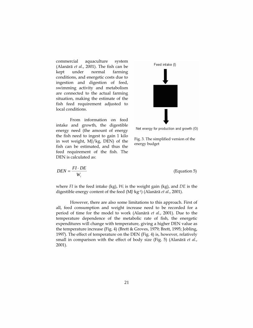
21

commercial aquaculture system (Alanärä et al., 2001). The fish can be kept under normal farming conditions, and energetic costs due to ingestion and digestion of feed, swimming activity and metabolism are connected to the actual farming situation, making the estimate of the fish feed requirement adjusted to local conditions.

From information on feed

intake and growth, the digestible energy need (the amount of energy the fish need to ingest to gain 1 kilo in wet weight, MJ/kg, DEN) of the fish can be estimated, and thus the feed requirement of the fish. The DEN is calculated as:

iWDEFIDEN ⋅

= (Equation 5)

where FI is the feed intake (kg), Wi is the weight gain (kg), and DE is the digestible energy content of the feed (MJ·kg-1) (Alanärä et al., 2001).

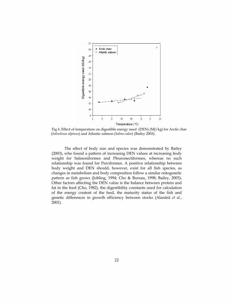
However, there are also some limitations to this approach. First of

all, feed consumption and weight increase need to be recorded for a period of time for the model to work (Alanärä et al., 2001). Due to the temperature dependence of the metabolic rate of fish, the energetic expenditures will change with temperature, giving a higher DEN value as the temperature increase (Fig. 4) (Brett & Groves, 1979; Brett, 1995; Jobling, 1997). The effect of temperature on the DEN (Fig. 4) is, however, relatively small in comparison with the effect of body size (Fig. 5) (Alanärä et al., 2001).

Fig. 3. The simplified version of the energy budget

22

The effect of body size and species was demonstrated by Bailey

(2003), who found a pattern of increasing DEN values at increasing body weight for Salmoniformes and Pleuronectiformes, whereas no such relationship was found for Perciformes. A positive relationship between body weight and DEN should, however, exist for all fish species, as changes in metabolism and body composition follow a similar ontogenetic pattern as fish grows (Jobling, 1994; Cho & Bureau, 1998; Bailey, 2003). Other factors affecting the DEN value is the balance between protein and fat in the feed (Cho, 1982), the digestibility constants used for calculation of the energy content of the feed, the maturity status of the fish and genetic differences in growth efficiency between stocks (Alanärä et al., 2001).

Fig 4. Effect of temperature on digestible energy need (DEN) (MJ/kg) for Arctic char (Salvelinus alpinus) and Atlantic salmon (Salmo salar) (Bailey 2003).

23

2.3 Growth models To measure growth in fish, increase in length or weight is usually

used (Wootton, 1998; Bureau et al., 2000). The simplest method of reporting growth is the absolute increase in weight or absolute growth (GA): GA = Wt-Wi (Equation 6) where Wt is the weight at time t and Wi is the initial weight (Ricker, 1979; Hopkins, 1992). Comparisons between experimental treatments using absolute growth rates are subject to two severe restrictions. First, the initial average size of the fish must be the same in all treatments (unless initial size differences are accounted for by statistical techniques such as randomized block designs or analysis of covariance). Second, the length of the experimental periods must be the same (Hopkins, 1992). This measurement of observed growth can be standardized to absolute growth

Fig. 5. Effect of body weight (g) on digestible energy need (DEN) (MJ/kg) for Salmoniformes, Perciformes and Pleuronectiformes (Bailey 2003).

24

rate (GG) by considering the number of days the experiment was performed:

tWWG it

G ∆−

= (Equation 7)

where Wt is the weight at time t, Wi is the initial weight and ∆t is the duration of the experiment (Winberg, 1971; Ricker, 1979; Knights, 1985; Hopkins, 1992). This implies that the relationship between time and weight is linear and that absolute growth rate is the same regardless of size of the fish. However, fish growth rate varies with size of the fish. A relative growth rate (GRR) will allow comparisons between treatments with fish of different initial sizes (Hopkins, 1992). The relative growth (GR) and relative growth rate (GRR) is expressed mathematically as:

i

itR W

WWG

−= (Equation 8)

tWWW

Gi

itRR ∆

−=

* (Equation 9)

where Wt is the weight at time t, Wi is the initial weight and ∆t is the duration of the experiment (Ricker, 1979; Hopkin,s 1992). Relative growth rates are typically used in fish nutrition studies and are reported as percent increase in weight per time unit. However, a relative growth rate is restricted to the length of time for which it was computed and cannot easily be converted to another time period (Hopkins, 1992).

2.3.1 Specific growth rate (SGR) To eliminate the problem with time in relative growth rates,

another exponential growth rate model is recommended, the instantaneous relative growth rate (GI) (Ricker, 1979; Hopkins, 1992). The instantaneous relative growth rate is usually shortened to instantaneous growth rate, but has also been referred to as specific, intrinsic, exponential, and logarithmic or compound interest rate (Ricker, 1979).

tGit

IeWW ∆= ** (Equation 10)

25

where Wt is the weight at time t, Wi is the initial weight, GI is the instantaneous growth rate and ∆t is the duration of the experiment (Ricker, 1979; Hopkin,s 1992). By transforming the equation and multiplying the growth rate by 100 one obtains the most commonly used measurement of growth, the specific growth rate, SGR (Hopkins, 1992; Jobling, 1994; Cho & Bureau, 1998; Bureau et al., 2000; Cui & Xie, 2000). SGR is expressed mathematically as:

100*lnln

tWW

SGR it

∆−

= (Equation 11)

where Wt is the weight at time t, Wi is the initial weight and ∆t is the duration of the experiment. SGR thus express the growth rate per unit weight of the fish as % weight increase/ unit time (days) (Winberg, 1971; Ricker, 1979; Knights, 1985; Hopkins, 1992; Cho & Bureau, 1998; Bureau et al., 2000; Cui & Xie, 2000; Alanärä et al., 2001).

The form of the equation assumes that fish weight increases exponentially. However, this assumption is only valid for most young fish cultured for short periods. SGR is thus particularly useful for reporting growth of small fish, but it is clearly not suitable for larger fish (Fig. 6) or longer culture periods (Hopkins, 1992).

2.3.2 Daily growth coefficient (DGC) To eliminate the problem with the decline in SGR with increasing

body size, Iwama & Tautz (1981) developed another growth index, the daily growth coefficient (DGC).

100*)3/1()3/1(

tWW

DGC it

∆−

= (Equation 12)

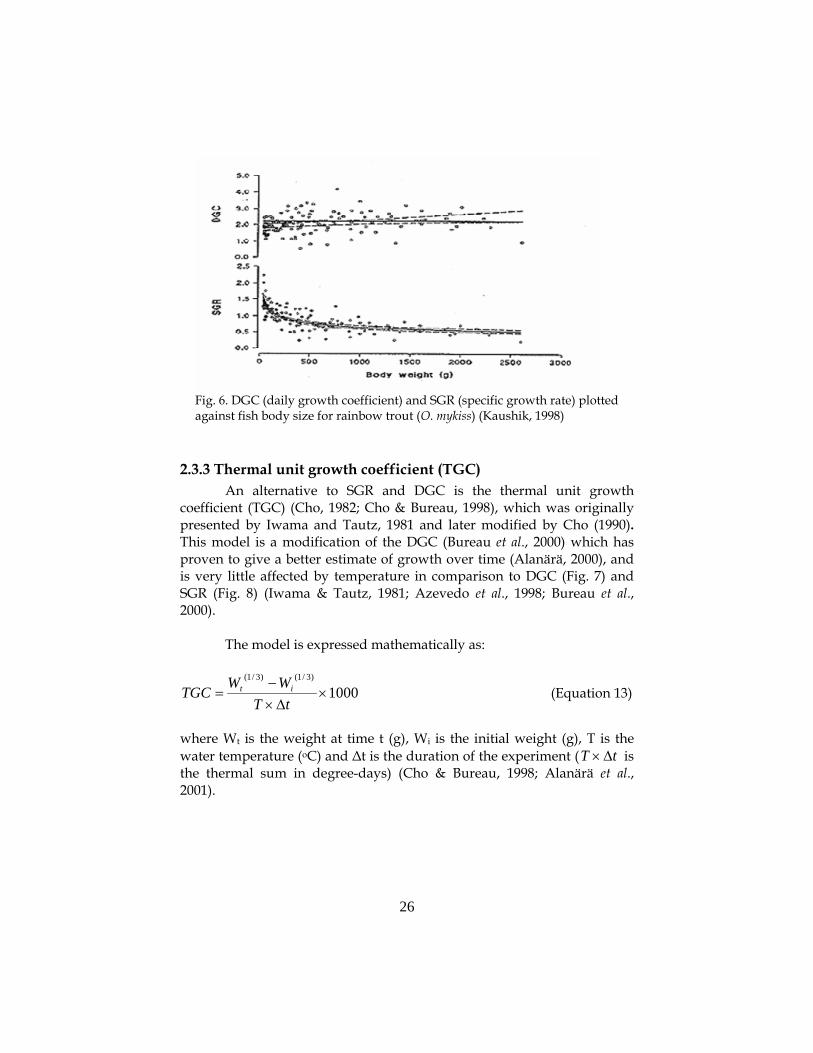
where Wt is the weight at time t, Wi is the initial weight and ∆t is the duration of the experiment (Iwama & Tautz, 1981; Bureau et al., 2000). One major advantage with DGC is that at a given temperature, the index is independent of fish body weight (Fig. 6). This has been validated for rainbow trout (Oncorhynchus mykiss) (Kaushik, 1998), common carp (Cyprinus carpio carpio) (Kaushik, 1995), and marine species in general (Kaushik, 1998). However, DGC is still affected by temperature (Fig. 7).

26

2.3.3 Thermal unit growth coefficient (TGC) An alternative to SGR and DGC is the thermal unit growth

coefficient (TGC) (Cho, 1982; Cho & Bureau, 1998), which was originally presented by Iwama and Tautz, 1981 and later modified by Cho (1990). This model is a modification of the DGC (Bureau et al., 2000) which has proven to give a better estimate of growth over time (Alanärä, 2000), and is very little affected by temperature in comparison to DGC (Fig. 7) and SGR (Fig. 8) (Iwama & Tautz, 1981; Azevedo et al., 1998; Bureau et al., 2000).

The model is expressed mathematically as:

1000)3/1()3/1(

×∆×−

=tT

WWTGC it (Equation 13)

where Wt is the weight at time t (g), Wi is the initial weight (g), T is the water temperature (oC) and ∆t is the duration of the experiment ( tT ∆× is the thermal sum in degree-days) (Cho & Bureau, 1998; Alanärä et al., 2001).

Fig. 6. DGC (daily growth coefficient) and SGR (specific growth rate) plotted against fish body size for rainbow trout (O. mykiss) (Kaushik, 1998)

27

Compared to SGR, which uses the logarithm of the final body weight of the fish to calculate the growth rate, TGC uses a power function (W(1/3)), as this mathematical adjustment of the growth model gives a better fit of the model to the actual growth pattern of the fish. From equation 13, the final body weight (Wt) of a fish can thus be calculated once the TGC value for the fish is known.

3)3/1(

1000⎟⎠⎞

⎜⎝⎛ ∆××+= tTTGCWW it (Equation 14)

Fig. 7. DGC and TGC for rainbow trout (O. mykiss) as a function of temperature (Bureau et al., 2000)

28

2.3.4 Pros and cons with growth models As an animal increases in size, the rate of its metabolic activities

slows down, and as a result, the relative growth rate (GR) will decline as the fish becomes larger (Ricker, 1979). It is also quite obvious that any increase in growth is relatively smaller for large fish than for small fish. This makes the relative growth rate unsuitable for comparing growth rates for fish of different sizes (Jobling, 1994). Moreover, the relative growth rate is, as mentioned earlier, restricted to the length of time for which it was computed and cannot be easily converted to another time period (Hopkins, 1992).

Specific growth rate (SGR) is also dependent on fish body size, and will decrease as the size of the fish increases (Fig. 6) (Hokanson, 1977; Iwama & Tautz, 1981; Jobling, 1994; Bureau et al. 2000). Another problem with SGR is also that this type of index has a tendency to overestimate predicted fish body weight if used to estimate a body weight that is greater than the largest body weight used for the construction of the model (Cho & Bureau, 1998).

The problem with comparing the growth rate estimate at

experimental periods of different length is, however, eliminated for the SGR as the index refers to a particular instant of time rather than to a time interval (Ricker, 1979). However, as temperature is not considered in the model (Fig. 8), the effect of temperature on growth has to be evaluated by collecting data for fish of different body sizes reared at different

0 2 4 6 8 10 12 14 160,00,51,01,52,02,53,03,54,0

SGR

10 g

100 g

1000 g

0 2 4 6 8 10 12 14 160,00,51,01,52,02,53,03,54,0

TGC

Temperature (oC) Temperature (oC)

10 g100 g1000 g

Fig. 8. The effect of temperature on the specific growth rate (SGR) and thermal unit growth coefficient (TGC) for arctic char (S. alpinus) (Jörgensen et al., 1991).

29

temperatures. This makes data collection both very time consuming and labour demanding, and as a consequence, only a few models describing SGR for fish in culture are available (Alanärä et al., 2001).

The daily growth coefficient (DGC) however, produces a relatively

constant growth rate regardless of the weight of the fish or the time interval between weightings, as the slope of the cubic root vs. time is the same (Bureau et al., 2000). This makes DGC better suited for dealing with data from fish of different body sizes than SGR (Fig. 6) (Kaushik, 1998). Unfortunately, temperature is not considered in this growth model either. The slope of the DGC will increase linearly with temperature (Fig. 7) (Iwama & Tautz, 1981), making the DGC, as are the SGR, best suited for data collected at a given temperature (Kaushik, 1998).

One way to overcome the problem with temperature is the thermal unit growth coefficient (TGC). The TGC has proven to be stable over a wide range of temperatures (Fig. 7) for several species (Iwama & Tautz, 1981; Azevedo et al., 1998; Cho & Bureau, 1998; Alanärä, 2000; Bureau et al., 2000; Alanärä et al., 2001). TGC is also less affected by fish size, (Kaushik, 1998) and time interval between weightings than other growth rate estimates such as SGR and DGC, and thus offer a simple model for growth rate comparisons (Bureau et al., 2000). The statement that TGC is unaffected by body size is, however, opposed by Alanärä (2000) who claims that the TGC value is not completely independent of body size, but increases with increasing body size.

Values of TGC might also vary with feed, husbandry, environment (Cho, 1990; Cho & Bureau, 1998; Alanärä et al., 2001) and with season (Fig. 9). As a general trend, TGC increases during spring and declines in autumn (Alanärä, 2000). This decline in autumn is not dependent on temperature or day length, but will occur even though the fish is held under constant conditions (Tveiten et al., 1996; Alanärä, 2000).

30

Once the TGC value is known, the growth model will provide

rather accurate estimates of growth in a variety of temperatures and to some extent for varying sizes of fish. Moreover, it is very easy for the farmer to obtain his or her own value of this coefficient, and thus obtain a model adjusted to local farm conditions (Alanärä, 2000). The TGC model can, if used with caution, allow comparisons between different culture operations, fish strains, production years, sampling intervals, etc, and can also be used in scientific studies to determine if fish have achieved their growth potential or determine the effect of different dietary and environmental factors (Bureau et al., 2000).

The biggest general draw back with growth models is that only a few models have been validated rigorously. This is a source of concern as if a model fails to predict fish growth under laboratory conditions, one should not expect it to work under field or aquaculture conditions either (Cui & Xie, 2000). The TGC model has to date only been validated for salmonids, but preliminary observations suggest that it is also valid for some non-salmonid species, for example, Nile tilapia (Oreochromis nilotica) (Bureau et al., 2000).

Fig 9. Growth of perch (P. fluviatilis) over season in 15ºC and natural day length (diamonds, from (Karås, 1990)) and in 17 ºC and constant day length (squares), from (Staffan, 2004).

31

3. FACTORS AFFECTING GROWTH AND ENERGY REQUIREMENTS

Growth of fish is governed by a variety of environmental factors including water temperature (Eckert, 1988; Elliot, 1994; De Silva & Anderson, 1995), photoperiod and light (Kestemont & Baras, 2001), dissolved oxygen concentration (De Silva & Andersson, 1995), unionized ammonia concentration (Colt & Tchobanoglous, 1978), feed availability and ration size (Brett, 1971; Elliot, 1994), type of feed (Eckert, 1988), season (Eckert, 1988) and salinity (De Silva & Anderson, 1995), as well as internal factors such as body size (Eckert, 1988; Elliot ,1994; De Silva & Anderson, 1995), genotype (Brett, 1979; Cuenco et al., 1985), cycles (De Silva & Anderson, 1995), stress (Eckert, 1988; De Silva & Anderson, 1995), age and sex (Eckert, 1988).

3.1 Temperature

Fish are obligate poikilotherms (ectotherms) (Elliot, 1994; De Silva & Anderson, 1995; Begon et al., 1996; Wootton, 1998). In contrast to endotherms, ectothermic animals rely on external sources of heat to maintain their body temperature (Eckert, 1988). Their gills are affective heat exchangers, but most heat transfer takes place directly through the body wall (Elliot, 1994), and as a consequence, the body temperature of fish fluctuates in close correspondence to the ambient water temperature (Ricker, 1979; De Silva & Anderson, 1995; Jobling, 1997). The surrounding water temperature will thus influence the fish behaviour (reproduction, activity, feeding and distribution) (Jobling, 1997), and physiological processes (hormone production and enzyme activity) (Eckert, 1988; Elliot, 1994; Jobling, 1995), and through these, metabolic rate (Cho & Bureau, 1998) and growth of the fish (Brett, 1979; Jobling et al., 1993).

3.1.1 Growth and feed intake Generally, feed intake, growth rate and growth efficiency will

increase with increasing temperature to a maximum close to the species optimum temperature4, and then decrease when temperature is increased

4 The temperatures at which feed intake, ingestion rate, growth efficiency and growth rate are maximized are often defined as the optimum temperature for the respective factor (Jobling, 1981).

32

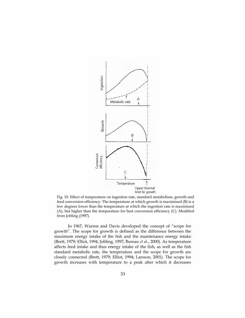
further and approach the species upper thermal tolerance limit5 (Jobling et al., 1993; Elliot, 1994; Jobling, 1994; Jobling, 1997; Wootton, 1998; Alanärä et al., 2001). However, the temperature at which energy (feed) intake for fish is maximized does not always correspond to the optimum temperature for growth of the fish (Jobling, 1997; Larsson, 2002). Optimum temperature for growth is usually slightly lower than the temperature at which feed intake is highest, but slightly higher than that corresponding to the best feed conversion efficiency (Fig. 10) (Cox & Coutant, 1981; Jobling, 1994; Brett, 1995; Jobling, 1997; Larsson, 2002). This is due to the exponential increase in maintenance energy cost6 as temperature increases (Jobling, 1994; Brett, 1995; De Silva & Anderson, 1995; Jobling, 1997; Cui & Xie, 2000), which show no decline as the temperature approaches the fish temperature tolerance limit (Ricker, 1979; Jobling, 1994; Brett, 1995; Jobling, 1997). The connection between temperature, feed intake and growth rate has been demonstrated for a number of species such as sockeye salmon (Oncorhynchus nerka) (Brett, 1979), perch (P. fluviatilis) and roach (Rutilus rutilus) (Lesmark, unpublished data). However, attempts to generalize should be treated with care as other species have shown no such connections in similar experiments (Forseth & Jonsson, 1994).

5 The thermal tolerance limits are the upper and lower temperature limits that a fish can handle. Outside these limits (lower temperatures than the lower, and higher temperatures than the higher), the fish will eventually die (Wootton, 1998). 6 Energy required by the fish to maintain all bodily functions without gaining or loosing weight ( Warren & Davis, 1967; Brett, 1979; Elliot, 1994; Jobling, 1997; Bureau et al. 2000).

33

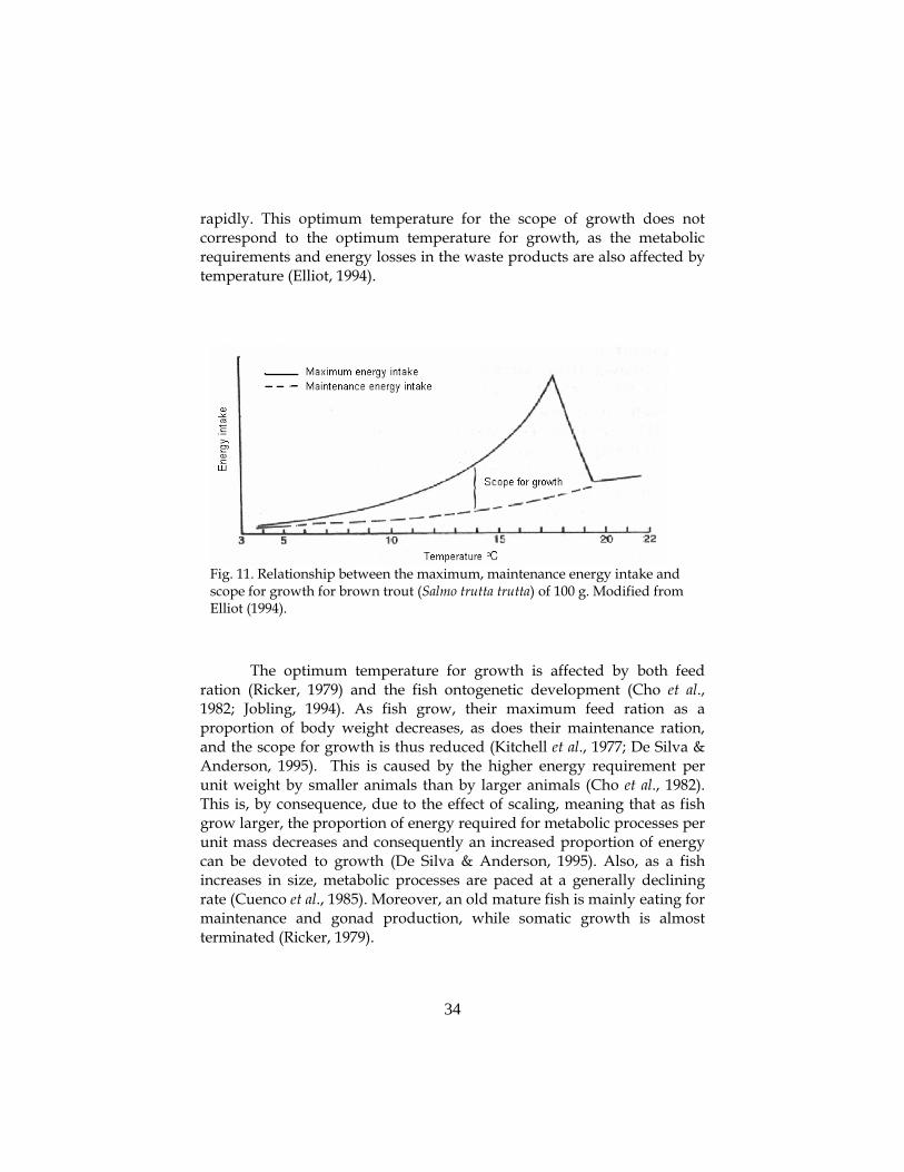
In 1967, Warren and Davis developed the concept of “scope for

growth”. The scope for growth is defined as the difference between the maximum energy intake of the fish and the maintenance energy intake (Brett, 1979; Elliot, 1994; Jobling, 1997; Bureau et al., 2000). As temperature affects feed intake and thus energy intake of the fish, as well as the fish standard metabolic rate, the temperature and the scope for growth are closely connected (Brett, 1979; Elliot, 1994; Larsson, 2001). The scope for growth increases with temperature to a peak after which it decreases

Fig. 10. Effect of temperature on ingestion rate, standard metabolism, growth and feed conversion efficiency. The temperature at which growth is maximized (B) is a few degrees lower than the temperature at which the ingestion rate is maximized (A), but higher than the temperature for best conversion efficiency (C). Modified from Jobling (1997).

34

rapidly. This optimum temperature for the scope of growth does not correspond to the optimum temperature for growth, as the metabolic requirements and energy losses in the waste products are also affected by temperature (Elliot, 1994).

The optimum temperature for growth is affected by both feed

ration (Ricker, 1979) and the fish ontogenetic development (Cho et al., 1982; Jobling, 1994). As fish grow, their maximum feed ration as a proportion of body weight decreases, as does their maintenance ration, and the scope for growth is thus reduced (Kitchell et al., 1977; De Silva & Anderson, 1995). This is caused by the higher energy requirement per unit weight by smaller animals than by larger animals (Cho et al., 1982). This is, by consequence, due to the effect of scaling, meaning that as fish grow larger, the proportion of energy required for metabolic processes per unit mass decreases and consequently an increased proportion of energy can be devoted to growth (De Silva & Anderson, 1995). Also, as a fish increases in size, metabolic processes are paced at a generally declining rate (Cuenco et al., 1985). Moreover, an old mature fish is mainly eating for maintenance and gonad production, while somatic growth is almost terminated (Ricker, 1979).

Fig. 11. Relationship between the maximum, maintenance energy intake and scope for growth for brown trout (Salmo trutta trutta) of 100 g. Modified from Elliot (1994).

35

The definition of the optimum temperature for growth is only valid if feed is not limited (Jobling, 1981). From the scope of growth models it can be seen that at limited rations, the greatest scope for growth, the fastest growth and most efficient feed conversion will occur at low temperatures (Hokanson, 1977; Ricker, 1979; Cox & Coutant, 1981; Jobling, 1994; Jobling, 1997), and as feed supply is increased, growth rate will increase and feed conversion decrease at higher temperatures (De Silva & Anderson, 1995; Jobling, 1997). As temperature increases towards the species upper tolerance limit for growth, the optimal feeding rate will approach the maximum feeding rate (Jobling, 1994). Moreover, as the feeding rate increases towards the maximum rate, the food conversion ratio will decrease from the maintenance ration to the optimum feeding rate and then increases to the maximum rate of feeding (Fig. 12). It is clear that there is a economic advantage in identifying and feeding fish at the optimal rate (De Silva & Anderson, 1995).

3.1.2 Temperature and growth modelling Due to its effects on fish physiology, temperature is a major factor

to consider when constructing growth models. To fit data to a model dealing not only with the increase in growth or ingestion rate as

Fig. 12. Relationship between growth rate, feeding rate and food

conversion ratio. Modified from De Silva & Andersson (1995).

36

temperature increase, but also with the decline occurring at higher temperatures is problematic (Elliot, 1994; Jobling, 1997). Frequently, the exponential, the logistic, or some related mathematical forms may be usefully fitted to describe the growth of fish. These models can easily be derived to describe fish growth with only the initial and final weight of fish during a certain time period. However, the use of the exponential growth model for long time periods is not recommended (Cuenco et al., 1985). Nevertheless, its use in aquaculture is relatively common because of its simplicity. Considering the whole life of a fish, the growth can conveniently be divided into a series of stages. The change from one stage to the next is characterized by some kind of crisis or discontinuity in development, such as hatching or maturation, or seasonal shifts in temperature for fish in temperate environments. Within any stage, increase in size may follow an s-shaped curve. For short periods of time, growth can thus be described by an exponential curve (Ricker 1979).

3.2 Season and Latitude

A number of fish species are distributed over a wide range of latitudes, and different populations inhabit environments that differ in both mean annual temperature and length of the growing season (Conover & Present, 1990; Williamson & Carmichael, 1990; Philipp & Whitt, 1991). Fish growth in temperate regions varies seasonally, and is usually faster in summer with a slowing down or cessation of growth during winter (MacCrimmon et al., 1971; Pitcher & Macdonald, 1973; Ricker, 1979). These variations in growth are often related to seasonal patterns of temperature and are therefore referred to as seasonal growth oscillations (Springborn et al., 1994). Moreover, for many species, populations at low latitudes grow faster than those in high latitudes in natural environments, due to the warmer climate and food availability all year around. However, when reared under the same conditions, fish from high latitudes sometimes grow faster than do low latitude populations, suggesting some form of growth rate compensation in high latitude populations (Karås, 1990; Wieser & Medgyesy, 1991; Conover & Schultz, 1995; Jobling, 1997; Craig, 2000; Larsson, 2002). As an example, Mandiki et al. (2004) found that survival and growth of perch (P. fluviatilis) larvae from different latitudinal areas differed in intensive culture systems, with northern juveniles having higher growth rates, higher feed intake and higher feed efficiency than fish from southern stocks.

37

There are two models explaining this phenomenon: the thermal adaptation model (TAM) and the countergradient model (CM) (Karås, 1990; Wieser & Medgyesy, 1991; Conover & Schultz, 1995; Jobling, 1997; Craig, 2000; Larsson, 2002). The TAM states that fish inhabiting areas with low annual mean temperature have a lower optimum temperature for growth, and grow faster at low temperatures, than do fish from populations living in areas with higher mean annual temperature (Karås, 1990; Wieser & Medgyesy, 1991; Jobling, 1997; Craig, 2000). The CM states that high latitude fish have a higher capacity for growth to compensate for the short growing season, rather than for low temperatures, which could be seen as an elevation of the growth rate-temperature curve compared to the curve for low latitude fish (Karås, 1990; Wieser & Medgyesy, 1991; Conover & Schultz, 1995; Jobling, 1997; Craig, 2000; Larsson, 2002).

3.3 Photoperiod and endogenous clock

Photoperiod or day length is known to influence both the feeding and growth of fish, but as it follows similar cycles to temperature, the effects of the two variables are often confused. For fish that feed visually, long periods of light is expected to increase the time at which the fish can forage, and a relationship between day length, growth and feed intake can be expected. Both the direction of changes (increasing/decreasing day length) (Jobling, 1994; Kestemont & Baras, 2001), the rate of change (Jobling, 1994) and the length of the light period (long/short day) (Huh et al., 1976; Hokanson, 1977; Ricker, 1979; Wieser & Medgyesy, 1991; Kestemont & Baras, 2001) can influence the growth and feed intake of a range of species. Typically, feed intake and growth increase at increasing day length prior to mid-summer and decrease towards autumn with gradually shorter day-length. This is known as the start of a winter depression in feed intake and growth (Ricker, 1979; Higgins & Talbot, 1985; Jobling, 1994).

The mechanisms behind these seasonal variations in feeding are

believed to be controlled by endogenous rhythms (Ricker, 1979). Evidence of endogenous annual cycles in growth and feed intake are convincing in many fish species (Jobling, 1994), especially in salmonids (Lundqvist et al., 1986) and in perch (P. fluviatilis) (Staffan, 2004). Photoperiod probably act as a time cue (Eriksson & Lundqvist, 1982), regulating the transition from slow growth in winter to fast growth in summer, and vice versa, while temperature control the growth rate within the respective periods (Karås, 1990). Seasonal changes in feed intake thus occur regularly, and can be

38

predicted in feed management plans (Alanärä et al., 2001). Another trigger for reduced feeding during the autumn may be the level of fat deposits. In order to decrease predation risk, fish stop feeding when they have enough fat reserves to survive the winter (Tveiten et al., 1996). Seasonal variations in feed intake have also been shown to relate to life history events in some species such as Atlantic salmon (S. salar) (Kadri et al., 1996).

Light intensity also affects the behaviour of fish, with threshold intensities varying between species (Kestemont & Baras, 2001). The suitable light level for efficiently foraging is about 100-200 lux for Atlantic salmon (S. salar) (Fraser & Metcalfe, 1997). However, 200 lux is a very low light intensity for farm personnel to work in. Nevertheless, the light intensity should not exceed 500 lux (Brännäs et al., 2001). Moreover, changes in light intensity may result in a shift from one preferred feed object to another (Kestemont & Baras, 2001), increase activity of the fish (Staffan, 2004), or modify feeding behaviour and efficiency of feed detection (Kestemont & Baras, 2001).

3.4 Water chemistry

Obviously, growth is also affected by several other factors such as salinity, water quality (ammonium levels) and oxygen levels (Ricker, 1979; Elliot, 1994; Rasmussen & Korsgaard, 1996). Deficiency in oxygen or elevated ammonium levels may reduce appetite of fish and thus affect feed intake and growth (Alanärä et al., 2001).

Salinity acts by constantly requiring some energy expenditures

associated with active transport of ions and osmotic regulation to maintain the proper ionic concentrations in the fish body fluids (Brett, 1979; Elliot, 1994; Jobling, 1994). The salinity level at which the fish is considered to be isoosmotic with the environment is about 8 ppt (Jobling, 1994). For perch (Perca fluviatilis), which is a freshwater fish but also commonly found in brackish areas, larval survival is higher in low salinity levels (0,6 and 1,2 ppt) compared to survival in freshwater (Bein, 1994). Juvenile growth is also enhanced by low salinity levels (2 and 5 ppt) compared to growth in freshwater (Lozys, 2004). In an aquaculture situation, the external environment should therefore be manipulated to ensure a reduction of metabolic costs connected to ionic- and osmoregulation and thus ensure an improved growth and feed utilisation of the fish (Jobling, 1994).

39

However, for some species, feed intake and growth rates reach a maximum at the mid point of a species salinity tolerance range (Kestemont & Baras, 2001). For example sea bass (Dicentrarchus labrax), which is eurhyaline and common in estuaries, grow better in intermediate salinity levels (15-28 ppt) compared to high (35-37 ppt) or low (8 ppt) salinity levels (Saillant, 2003; Conides, 2004). Black sea bass (Centropristis striata) are usually found in waters with salinity levels of 30-35 ppt, and it has been demonstrated that survival and development of both early life stages (larvae) and juveniles are favoured by high salinity levels (20-30 ppt) (Cotton, 2003; Berlinsky, 2004). Cod (Gadus morhua), a species found in marine and brackish areas, has a higher growth rate in intermediate (14 ppt) than in low (7 ppt) or high (28 ppt) salinity levels (Lambert et al., 1994). Information about salinity requirements for rainbow trout (O. mykiss), which can be both anadromous or freshwater living, is confusing. Feed intake is reported to increase from freshwater to 15-28 ppt and then decrease if salinity is increased further (MacLeod, 1977), but growth is reported to decrease as salinity is increased from 0 to 32 ppt (Juerss, 1985; McKay & Gjerde, 1985). This is however opposed by Tsintsadze (1991), who detected an increase in growth rate for rainbow trout in 18 ppt compared to in freshwater. Salinity manipulations should therefore not be used as a growth enhancing method unless convincing data concerning the efficiency of the manipulation exist for the target species.

3.5 Biotic factors

There are also numerous biotic factors affecting the growth performance of fish in aquaculture. The two main causes of reduced or heterogenic growth in farming conditions are genetic variation and social interactions (Mélard et al., 1995; Bureau et al., 2000; Brännäs et al., 2001). Other important factors are the type of feed available (Craig & Kipling, 1983), feed management (Mélard et al., 1995; Bureau et al., 2000), age of maturity (Craig, 2000), sexual dimorphism (Malison et al., 1986; Kestemont & Mélard, 2000) and stress (Knights, 1985; Jobling, 1994; Lindberg, 2001). In order to ensure that the fish are able to display growth rates close to their physiological potential, it is essential to have information about the ways in which various biotic factors can influence feed intake and growth performances of individual fish within larger groups (Jobling, 1994).

3.5.1 Group dynamics and social interactions The social environment of fish is influenced by factors such as size

heterogeneity, sex and sex ratio. The initial establishment of a social

40

hierarchy does not require size differences between fish, but hierarchies may be promoted by size heterogeneity (Kestemont & Baras, 2001). To some extent, variations in feed intake and growth can be caused by these social interactions and dominance hierarchies, with suppressed feed intake in subordinate fish due to territory formations and feed source monopolization (Alanärä & Brännäs, 1993; Jobling, 1994; De Silva & Anderson, 1995; Alanärä & Brännäs, 1996; Kestemont & Mélard, 2000; Brännäs et al., 2001). Moreover, competitors that gain early access to food may have digested their meal and can feed again before the end of the feeding period, whereas this opportunity is denied to fish that ingest their first meal later. The monopolisation of food by dominants is usually greatest at low input rates (Brännäs & Alanärä, 1994), at time restricted access to feed, and at low rearing densities (Kestemont & Baras, 2001).

However, as group size increases, territorial behaviour becomes

less profitable as resources are hard to defend in crowded environments. Thus, at sufficiently large group sizes, the fish may form schools or looser aggregations, and territorial and agonistic behaviour is reduced (Jörgensen et al., 1993; Jobling, 1994; Brännäs et al., 2001; Kestemont & Baras, 2001). For some species, high stocking densities may lead to increased survival, better growth and reduced size heterogeneity within a population (Nile tilapia (O. niloticus) (Mélard, 1986), Arctic charr (S. alpinus) (Jörgensen et al., 1993), sharptooth catfish (Clarias gariepinus) (Kaiser et al., 1995), perch (P. fluviatilis) (Mélard et al., 1996)). Despite this, high stocking density is often considered to be a stressor for fish, with resulting detrimental effects on feeding, growth and a range of physiological processes. However, these effects are often caused by deterioration of water quality, or reduced adequacy of food distribution, rather than them being a direct consequence of an increase in stocking density (Kestemont & Baras, 2001).

Another way to reduce agonistic behaviour between co-specifics and the occurrence of dominance hierarchies is to force the fish to swim at moderate speeds for prolonged periods of time (Christiansen & Jobling, 1990; Jobling, 1994; Kestemont & Baras, 2001; Lindberg, 2001). The energy cost of swimming is rather high, but the reduced waste of energy in agonistic behaviour as fish swim against the current still increase fish growth rates (Jobling, 1994; Brännäs et al., 2001). Consequently, the subordinates increase their growth rate either by an increase in their feed intake (Christiansen & Jobling, 1990) and/or by a decrease in their stress-

41

related metabolic costs (Adams et al., 1995). Moreover, fish exercising in moderate water currents frequently consume more food than unexercised fish (Leon, 1986; Totland et al., 1987; Jörgensen & Jobling, 1993). Moderate water currents may also result in improved feed distribution and better feeding conditions for the fish (Christiansen & Jobling, 1990; Jobling, 1994; Lindberg, 2001). However, excessive water velocities may reduce the ability of fish to capture passing food items (Flore & Keckeis, 1998). Additional reasons for faster growth and improved feed conversion efficiency may include the hypertrophy of the swimming muscle mass (Totland et al., 1987) and changes in rates of protein synthesis and deposition (increases in protein synthesis at the expense of fat deposition) (Houlihan & Laurent, 1987; Lindberg, 2001).

Stocking density may also affect the occurrence of cannibalism in some species. Conditions that increase the likelihood of cannibalism include low feed availability, high fish densities, large size variation and the absence of shelter (Brännäs et al., 2001).

3.5.2 Stress Stress has been defined in many different ways but mainly in

physiological terms (Brännäs et al., 2001). Examples of physiological signs of stress are elevated corticosteroid production, blood glucose, lactate levels and brain hormones (serotonin) (Winberg et al., 1993). The physiological systems of fish can be challenged or “stressed” by a wide range of biological, chemical and physical factors. The term stressor can be used to describe these factors if the disturbance is severe enough to elicit a compensatory physiological response. These responses can, in the long term, lead to a decrease in the condition of the fish, impair growth, reproductive performance or disease resistance by suppression of the immune system, increase the vulnerability of the fish to invading pathogens, and thus reduce survival of the fish (Knights, 1985; Jobling, 1994; Lindberg, 2001). Measuring stress of fish is difficult, but abnormal swimming behaviour, low swimming activity, low and variable growth, fin damage, wounds and scale loss and high numbers of external parasites are all easily detected signs of stress (Lindberg, 2001).

Fish in all environments will sometimes inevitable suffer from stressful conditions. However, fish held in aquaculture are very sensitive to “apparent” riskiness, and if they are frightened too often or subjected to constant threats, their feeding activity and growth may be affected.

42

Juveniles especially attempt to avoid environments that may put them at risk of predation, even if no real predator is present. Such conditions could include low water depths, high light intensities, light coloured tanks, lack of cover, and too frequent handling routines or inappropriate feeding regimes (De Silva & Anderson, 1995; Lindberg, 2001). Factors such as cleaning of tanks, disease treatments (Kestemont & Baras, 2001), quick changes in temperature, social dominance hierarchies or feeding and bad water quality may also expose the fish to a stressful situation (De Silva & Anderson, 1995; Brännäs et al., 2001).

It is generally believed that acute disturbance, such as weighting

or the transfer of fish from one rearing unit to another result in reduced feed intake for periods of several hours to days. Prolonged human activity near tanks may also affect fish in various ways. For example, perch (P. fluviatilis) that are disturbed by prolonged human activity during the early morning prior their first meal of the day reduce their feeding frequency over the entire day, and the daily ration is reduced to 40 % of that under normal conditions. However, if the fish are disturbed later in the day, after having fed, feeding resumes soon after the perturbation, and the daily ration is very little affected. Illumination from outside a rearing unit may generate shadows during human activity or bird passage, and this disturbance to the fish may result in cessation of feeding for several hours to days (Kestemont & Baras, 2001). Although it is well documented that stress affect fish appetite, very few quantitative data are available in this area (De Silva & Anderson, 1995).

3.5.3 Living conditions The living environment, i.e. colour of rearing tanks, is also of

importance for fish behaviour, growth, stress and welfare. Living conditions should mimic the natural conditions as much as possible. Dark tank colours are preferred by most species, whereas bright colours will create a marked contrast between the fish and tank surroundings, which is associated with high predation risk. Many fish species also have a need for hiding in different situations. This is mainly anti-predator behaviour that is very important for fish at different times of the day or season, or when the environment in general signals high predation risk. It would be desirable if an environment containing hiding areas for the fish was created, at least in intensive aquaculture in tanks. This can easily be achieved by covering a part of the tank with a plastic sheet, shading about 30-50 % of the tank area (Brännäs et al., 2001).

43

3.5.4 Feed management Growth is affected by feeding practises, and can be poor if the feed

is delivered sub optimally in time or space, or if feeding responses are suppressed as a result of the fish being stressed (Jobling, 1994; Brännäs et al., 2001). Some important factors to be considered when dealing with feed management are for example size of the daily ration (Bailey, 2003), the nutritional and physical status of the feed (Cho, 1990; Craig, 2000) and the method by which the feed is delivered (Cho, 1990; Bailey, 2003). Important factors to consider when delivering feed include time of day (Alanärä, 2000), number of meals (Ricker, 1979; Johansen & Jobling, 1998; Alanärä et al., 2001), the duration of a given feeding (satiation time) (Ricker, 1979; Alanärä, 2000), delivery rate (Alanärä et al., 2001), individual meal size (stomach capacity) (Brett, 1979; Brännäs, 2001; Bailey, 2003), time between meals (feeding frequency) (Ricker, 1979), spatial and temporal feed dispersal (Thorpe et al., 1990; Grant & Guha, 1993; Alanärä et al., 2001; Brännäs et al., 2001), and pellet size (Tabachek, 1988 ; Linnér & Brännäs, 1994; De Silva & Anderson, 1995; Bailey, 2003).

44

4. APPLICATIONS OF GROWTH MODELS WITH REFERENCE TO PERCH 4.1 Feed management

Feed cost is one of the highest cost in intensive and semi-intensive aquaculture, often reaching 40% of production costs (De Silva & Anderson, 1995; Cho & Bureau, 1998; Bailey, 2003). Many producers rely on feeding charts provided by feed manufacturers to determine the amount of feed needed by their stock (Cho, 1992; Alanärä, 2000; Bureau et al., 2000). As most feeding charts available today tend to overestimate feed requirement of the fish (Cho & Bureau, 1998), and as the energy requirement of fish vary with species, strains and with local conditions (Cho, 1992; Alanärä, 2000; Bureau et al., 2000), many culture operations end up with poor feed utilisation. The efficiency with which fish utilise the feed is a major factor determining the economic gain and thus the viability of the farm (Alanärä, 2000; Alanärä et al., 2001; Kestemont & Mélard, 2000). Accurate calculation of the daily food ration assures that maximum growth will be obtained without waste of food and unnecessary fouling of the water (Soderberg, 1992; Cho & Bureau, 1998; Alanärä et al., 2001). It is thus necessary to optimize feeding regimes to improve the economical and environmental sustainability of aquaculture (Cho & Bureau, 1998).

4.1.1 Feed conversion model One way of measuring the feed delivery efficiency is to use a feed

conversion ratio (FCR). The FCR describes the amount of feed used (kg) to produce 1 kg of fish (Knights, 1985; Alanärä, 2000). The FCR thus describes the efficiency of the farm to produce fish (not the efficiency with which the fish utilized the food), and can be expressed as:

PFdFCR = (Equation 15)

where Fd is the amount of feed delivered (kg) and P is the production of fish (kg) (final mass-initial mass) (Parker, 1987; Alanärä, 2000). This estimate is open to many errors as relationships between given feed and feed actually consumed are generally unknown (Knights, 1985). FCR for fish are also influenced by other factors such as species, age or size, sex, reproductive state, stocking density, water temperature, photoperiod,

45

feeding rate, feeding frequency, palatability and acceptance of the feed, time of year and time of day the fish is fed (Parker, 1987).

The ultimate goal is to achieve a FCR that is as low as possible, i.e. no or very little feed waste (Alanärä, 2000). In most intensive aquaculture systems where dry pellets are fed to the fish, the value of FCR ranges between 0.8 and 2.0 (Parker, 1987). Values of 1.1 to 2.0 have been obtained for perch ranging in size from 3 to 300 g (Kestemont & Mélard, 2000). In practical terms, the FCR quickly tells the producer how much feed he needs to give the fish to obtain a certain amount of weight gain of the fish. The value can thus be used to calculate feed costs per unit weight gain and to compare production costs for different feeds (Parker, 1987). The FCR can also be calculated theoretically as:

DENDEFCRt = (Equation 16)

where DE is the digestible energy content of the feed (MJ DE/kg) and DEN is the digestible energy need of the fish (MJ DE/kg) (the amount of energy (MJ) the fish need to ingest to increase 1 kilo in weight) (Equation 5) (Alanärä, 2000). This number gives an easy way to evaluate the efficiency of the feed management of a farm by comparing the actual FCR with the theoretically possible FCRt.

4.1.2 Feed budget model Another way to optimize fish production is to develop a feed

budget; a model describing the feed requirement of the fish (Alanärä, 2000). As feed intake of fish is controlled mainly by body weight, season, water temperature and energy content of the feed, the first step in estimating feed requirements is to predict the expected live weight gain of the fish in a given time period, under the given water temperature and management (Cho & Bureau, 1995). This can be done by using a growth model, for example the TGC (equation 13). The TGC must first be estimated from fish growth records from previous years, with the assumption that similar husbandry conditions and fish stock are used (Cho & Bureau, 1995; Cho & Bureau, 1998). Once the daily weight gain is estimated (equation 13), the digestible energy need (DEN) of the fish need to be estimated from previously

46

registered feed intake and growth of the fish (Equation 5). Information about the feed digestible energy content (DE: MJ·kg-1) is also required. In the absence of measured DE values, the values in table 2 can be used. The digestibility constants are species specific. For perch, the best estimate of the digestibility values are average of values obtained for European sea bass (D. labrax). Table 2. Digestible energy content of proteins, fat and carbohydrates. The digestibility coefficient shows how much of the energy is actually digested by the fish.

Substance Digestibility coefficient*

Energy (kJ/g) (Davidson et al., 1979; Cho et al., 1982)

Digestible energy content (kJ/g)

Protein 0,94 23,4 0,94*23,4 Fat 0,94 39,2 0,94*39,2 Carbohydrate 0,88 17,2 0,88*17,2 * Average for European sea bass (Dicentrarchus labrax) (Dias et al., 1998; Peres & Olivia-Teles, 2002; Webster& Lim, 2002)

The proportions of the substances in the diet can be determined by

chemical analysis. The energetic contribution of each substance to the total energy of the diet is then calculated by multiplying the proportion of a substance with its digestible energy content. For example, a manufactured feed contains 44% protein, 13 % fat and 25% carbohydrates. The digestible energy from protein will be: 0,94 * 23,4 * 0,44 = 9,7 The digestible energy from fat will be: 0,94 * 39,2 * 0,13 = 4,8 The digestible energy from protein will be: 0,88 * 17,2 * 0,25 = 3,8 The total digestible energy content of the feed will be:

9,7 + 4,8 + 3,8 = 18,3 kJ/g

From data published by Kestemont et al. (2001), the DEN value for perch can be estimated to range between 15,1 and 24,2 MJ/kg (or kJ/g) (Kestemont et al., 2001; Bailey, 2003; Strand et al., In prep.).

Once the DEN value has been obtained, the theoretical energy requirement (TER) (the amount of energy the fish need to ingest to obtain optimum growth under specific conditions) of the fish can be calculated from:

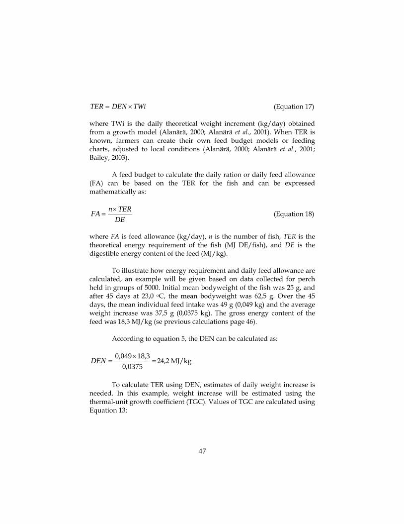
47

TWiDENTER ×= (Equation 17)

where TWi is the daily theoretical weight increment (kg/day) obtained from a growth model (Alanärä, 2000; Alanärä et al., 2001). When TER is known, farmers can create their own feed budget models or feeding charts, adjusted to local conditions (Alanärä, 2000; Alanärä et al., 2001; Bailey, 2003).

A feed budget to calculate the daily ration or daily feed allowance (FA) can be based on the TER for the fish and can be expressed mathematically as:

DETERnFA ×

= (Equation 18)

where FA is feed allowance (kg/day), n is the number of fish, TER is the theoretical energy requirement of the fish (MJ DE/fish), and DE is the digestible energy content of the feed (MJ/kg).

To illustrate how energy requirement and daily feed allowance are calculated, an example will be given based on data collected for perch held in groups of 5000. Initial mean bodyweight of the fish was 25 g, and after 45 days at 23,0 oC, the mean bodyweight was 62,5 g. Over the 45 days, the mean individual feed intake was 49 g (0,049 kg) and the average weight increase was 37,5 g (0,0375 kg). The gross energy content of the feed was 18,3 MJ/kg (se previous calculations page 46).

According to equation 5, the DEN can be calculated as:

=×

=0375,0

3,18049,0DEN 24,2 MJ/kg

To calculate TER using DEN, estimates of daily weight increase is

needed. In this example, weight increase will be estimated using the thermal-unit growth coefficient (TGC). Values of TGC are calculated using Equation 13:

48

10004523255,62 )3/1()3/1(

××−

=TGC = 1,01

Now, the farmer can calculate for example how much feed his fish

need during the coming week (7 days). Based on the TGC value calculated from previous growth data, the body weight of perch at 23 oC after seven days of growth can be calculated according to equation 14:

3)3/1( 723

100001,15,62 ⎟

⎠⎞

⎜⎝⎛ ××+=tW = 70,4 g

The theoretical daily weight increase (TWi) in kg is then:

TWi = 0,0704-0,0625 = 0,008 kg/7 days 0,001 kg/day

When DEN and TWi are known, the TER can be calculated according to Equation 17:

001,02,24 ×=TER = 0,0276 MJ/day

Finally, the daily feed allowance can be calculated according to Equation 18:

3,180276,05000×

=FA = 7,55 kg/day

The fish thus need 7,55 kg feed per day and tank to reach the target

average weight of 70,4 g in a week.

Another example is if the farmer want to predict how long time it will take for his fish to grow to market size of 150 g from a current weight of 100 g. As in the pervious example, we assume that the farmer keep the fish in 23 oC with 5000 fish per tank and give the fish a feed containing 18,3 MJ/kg feed.

By using equation 13, and the TGC value estimated from pervious growth data, the time can be estimated as:

49

100023

10015001,1)3/1()3/1(

××−

=Time

100001,123

100150 )3/1()3/1(

××−

=Time = 29 days

It is important, however, to point out that each farmer should try

to estimate his/hers own TGC and DEN values as no such data exist for commercial production of perch at this time. The data used in the calculations are estimations from laboratory experiments performed during summertime when the fish grows optimally.

50

REFERENCES Adams, C. E., Huntingford F. A., Krpal, J., Jobling, M. & Burnett, S. J. 1995.

Exercise, agnostic behaviour and food acquisition in Arctic charr, Salvelinus alpinus. Environmental Biology of Fishes, 43(2): 213-218.

Alanärä, A. 2000. Optimering av utfodring vid kommersiell fiskodling. Rapport No. 21. Institutionen för Vattenbruk, Umeå, SLU: 32.

Alanärä, A. & Brännäs, E. 1993. Monitoring the feeding activity of individual fish with a demand feeding system. Journal of Fish Biology, 42(2): 209-215.

Alanärä, A. & Brännäs, E. 1996. Dominance in demand-feeding behaviour in Arctic charr and rainbow trout: The effect of stocking density. Journal of Fish Biology, 48(2): 242-254.

Alanärä, A., Kadri, S. & Paspatis, M. 2001. Feeding management. In: Feed intake in fish. Houlihan, D., Jobling, M. & Boujard T. (Eds.), Blackwell Science, Oxford, UK: 332-353.

Allen, J. R. M. & Wootton, R. J. 1982. Age, growth and rate of food consumption in an upland population of the three-spined stickleback, Gasterosteus aculeatus (L.). Journal of Fish Biology, 21(1): 95-106.

Azevedo, P. A., Cho, C. Y., Leeson, S. & Bureau, D. P. 1998. Effects of feeding level and water temperature on growth, nutrient and energy utilization and waste outputs of rainbow trout (Oncorhynchus mykiss). Aquatic Living Resources, 11(4): 227-238.

Bailey, J. 2003. Energy Requirements and Feeding Behaviour of Salmonids in Culture. Doctoral Thesis. Department of Aquaculture. Swedish University of Agricultural Sciences, Umeå.

Begon, M., Harper, J. L. & Townsend, C. R. 1996. Ecology: Individuals, Populations and Communities. Blackwell Science Ltd., Milan.

Bein, R. & Ribi, G. 1994. Effects of larval density and salinity on the development of perch larvae (Perca fluviatilis L.). Aquatic Sciences, 56(2): 97-105.

Berlinsky, D. L., Taylor, J. C., Howell, R. A., Bradley, T. M. & Smith, T. I. J. 2004. The effects of temperature and salinity on early life stages of black sea bass Centropristis striata. Journal of the World Aquaculture Society, 35(3): 335-344.

Boehlert, G. W. & Yoklavich, M. M. 1983. Effects of temperature, ration, and fish size on growth of juvenile black rockfish, Sebastes melanops. Environmental biology of fishes, 8(1): 17-28.

51

Brafield, A. E. 1985. Laboratory studies of energy budgets. In: Fish energetics: new perspectives. Tytler, P. & Calow, P. (Eds.), Croom Helm Australia Pty Ltd., Sydney: 257-281.

Brett, J. R. 1962. Some considerations in the study of respiratory metabolism in fish, particularly salmon. Journal of Fisheries Research Board of Canada, 19: 1025-1038.

Brett, J. R. 1971. Satiation time, appetite, and maximum food intake of sockeye salmon (Oncorhynchus nerka). Journal of Fisheries Research Board of Canada, 28(3): 409-425.

Brett, J. R. 1979. Environmental factors and growth. In: Fish physiology. Hoar, W. S., Randall, D. J. & Brett, J. R. (Eds.), Academic Press Inc. Ltd., London, Vol. VIII.

Brett, J. R. 1995. Energetics. In: Physiological Ecology of Pacific Salmon. Groot, C., Margolis, L. & Clarke, W. C. (Eds.), UBC Press, Vancouver: 3-68.

Brett, J. R. & Groves, T. D. D. 1979. Physiological energetics. In: Fish physiology. Hoar, W. S., Randall D. J. & Brett, J. R. (Eds.) Academic Press Inc. Ltd., London, Vol. VIII.

Brännäs, E. & Alanärä, A. 1994. Effect of reward level on individual variability in demand feeding activity and growth rate in Arctic charr and rainbow trout. Journal of Fish Biology, 45(3): 423-434.

Brännäs, E., Alanärä, A. & Magnhagen, C. 2001. The Social Behaviour of Fish. In: Social behaviour in Farm Animals. Keeling, L. J. & Gonyou, H. W. (Eds.), CABI publishing, Wallingford: 275-304.

Bureau, D. P., Azevedo, P. A., Tapia-Salazar, M. & Cuzon, G. 2000. Pattern and cost of growth and nutrient deposition in fish and shrimp: Potential implications and applications. Avances en Nutrición Acuícola V, Mérida, Yucatán, Mexico, Fish nutrition research laboratory.

Calow, P. 1985. Adaptive Aspects of Energy Allocation. In: Fish energetics: new perspectives. Tytler, P. & Calow, P., Croom Helm Australia Pty Ltd., Sydney: 13-31.

Cho, C. Y. 1982. Effects of dietary protein and lipid levels on energy metabolism of rainbor trout (Salmo gairdneri). Energy metabolism of farm animals. Proceedings of the 9:th symposium, Lillehammer, Norway, European association for animal production.

Cho, C. Y. 1990. Fish nutrition, feeds, and feeding: with special emphasis on salmonid aquaculture. Food Reviews International, 6(3): 333-357.

52

Cho, C. Y. 1992. Feeding systems for rainbow trout and other salmonids with reference to current estimates of energy and protein requirements. Aquaculture, 100: 107-123.

Cho, C. Y. & Bureau, D. P. 1995. Determination of the energy requirements of fish with particular reference to salmonids. Journal of Applied Ichtyology, 11: 141-163.

Cho, C. Y. & Bureau, D. P. 1998. Development of bioenergetic models and the Fish-PrFEQ software to estimate production, feeding ration and waste output in aquaculture. Aquatic Living Resources, 11(4): 199-210.

Cho, C. Y. & Kaushik, S. J. 1985. Effects of protein intake on metabolizable and net energy values of fish diets. International Symposium on Feeding and Nutrition in Fish, Aberdeen, UK.

Cho, C. Y., Slinger, S. & Bayley, H. S. 1976. Influence of level and type of dietary protein, and of level of feeding on feed utilization by rainbow trout. Journal of Nutrition, 106(11): 1547-1556.

Cho, C. Y., Slinger, S. J. & Bayley, H. S. 1982. Bioenergetics of salmonid fishes: energy intake, expenditure and productivity. Comparative Biochemistry and Physiology, 73B (No. 1): 25-41.

Christiansen, J. S. & Jobling, M. 1990. The behaviour and the relationship between food intake and growth of juvenile Arctic charr, Salvelinus alpinus L., subjected to sustained exercise. Canadian Journal of Zoology 68(10): 2185-2191.

Colt, J. & Tchobanoglous, G. 1978. Chronic exposure of channel catfish, Ictalurus punctatus , to ammonia: effects on growth and survival. Aquaculture 15(4): 353-372.

Conides, A. J., Glamuzina, B. & Papaconstantinou, C. 2004. Labratory simulation of the effetcs of environmeltal salinity on wild-caught juveniles of European sea bass Dicentrarchus labrax and gilthead seabream Sparus aurata. Journal of Fish Biology, 65(supplement A): 326-336.

Conover, D. O. & Present, T. M. C. 1990. Countergradient variation in growth rate: compensation for length of the growing season among Atlantic silversides from different latitudes. Oceologica 83: 316-324.

Conover, D. O. & Schultz, E. T. 1995. Phenotypic similarity and the evolutionary significance of countergradient variation. TREE 10(6): 248-252.

Cotton, C. F., Walker, R. L. & Recicar, T. C. 2003. Effects of temperature and salinity on juvenile black sea bass, with implications for

53

aquaculture. North American Journal of Aquaculture, 65(4): 330-338.

Cox, D. K. & Coutant, C. C. 1981. Growth Dynamics of Juvenile Striped Bass as Functions of Temperature and Ration. Transactions of the American Fisheries Society 110: 226-238.

Craig, J. 1977. The body composition of adult perch, Perca fluviatilis in Windermere, with reference to seasonal changes and reproduction. Journal of Animal Ecology 46(2): 617-632.

Craig, J. F. 2000. Age, Growth and Mortality. Percid fishes. Systematics, Ecology and Exploitation. Pitcher, T. J. (Ed.), Blackwell Science, Dunscore, Scotland.

Craig, J. F. & Kipling, C. 1983. Reproduction effort versus the environment; Case histories of Windermere perch, Perca fluviatilis L., and pike, Esox lucius L. Journal of Fish Biology 22(6): 713-727.

Cuenco, M. L., Stickney, R. R. & Grant, W. E. 1985. Fish bioenergetics and growth in aquaculture ponds. Ecological Modelling 27(3-4): 169-206.

Cui, Y. & Wootton, R. J. 1989. Bioenergetics of growth of a cyprinid, Phoxinus phoxinus (L.): development and testing of a growth model. Journal of Fish Biology 34: 47-64.

Cui, Y. & Xie, S. 2000. Modelling Growth in Fish. Feeding Systems and Feed Evaluation Models. Theodorou, M. K. & France, J. (Eds.), CAB International: 413-434.

Davidson, S., Passmore, R., Brock, J. F. & Truswell, A. S. 1979. Human Nutrition and Dietetics. Churchill-Livingston, Edinburgh.

De Silva, S. S. & Anderson, T. A. 1995. Fish nutrition in Aquaculture. St Edmundsbury Press, Suffolk.

Dias, J., Huelvan, C., Dinis, M. T. & Métailler, R. 1998. Influence of dietary bulk agents (silica, cellulose, and natural zeolite) on protein digestibility, growth, feed intake and feed transit time in European seabass (Dicentrarchus labrax) juveniles. Aquatic Living Resources 11(4): 219-226.

Dufour, E. & Gerdeaux, D. 2001. Contribution of stable isotopes to fish ecological studies. Cybium, 25(4): 369-382.

Eckert, R. 1988. Animal Energetics and Temperature Relations. In: Animal Physiology, Mechanisms and Adaptions. Eckert, R.& Augustine, G. (Eds.) W. H. Freeman and Company, Los Angeles, 555-605.

Ege, R. & Krogh, A. 1914. On the relation between the temperature and the respiratory exchange in fishes. International Revue of Hydrobiology 1: 48-55.

54

Elliot, J. M. 1994. Quantitative Ecology and the Brown Trout. Oxford University Press, Oxford.

Eriksson, L.-O. &Lundqvist, H. 1982. Circannual rhythms and photoperiod regulations of growth and smolting in baltic salmon (Salmo salar). Aquaculture 28: 113-121.

Flore, L. & Keckeis, H. 1998. The effect of water current on foraging behaviour of the rheophilic cyprinid Chondrostoma nasus (L.) during ontogeny: Evidence of a trade-off between energetic gain and swimming costs. Regulated Rivers: Research and Management 14(1): 141-154.

Forseth, T. & Jonsson, B. 1994. The growth and food ration of piscivorous brown trout (Salmo trutta). Functional ecology 8: 171-177.

Fraser, N. H. C. & Metcalfe, N. B. 1997. The costs of becoming nocturnal: feeding efficiency in relation to light intensity in juvenile Atlantic salmon. Functional ecology 11(3): 385-391.

Grant, J. W. A. & Guha, R. T. 1993. Spatial clumping of food increases its monopolization and defence by convict cichlids, Cichlasoma nigrofasciatum. Behavioral Ecology 4(4): 293-296.

Griffiths, D., Kirkwood, R. C. 1995. Seasonal variation in growth, mortality and fat stores of roach and perch in Lough Neagh, Nortern Ireland. Journal of Freshwater Biology 47(3): 537-554.

Higgins, P. J. & Talbot, C. 1985. Growth and feeding in juvenile Atlantic salmon (Salmo salar L.). International Symposium on Feeding and Nutrition in Fish, Aberdeen, UK.

Hokanson, K. E. F. 1977. Temperature Requirements of Some Percids and Adaptations to the Seasonal Temperature Cycle. Journal of Fisheries Research Board Canada 34: 1524-1550.

Hopkins, K. D. 1992. Reporting Fish Growth: a Review of the Basics. Journal of the World Aquaculture Society 23(3): 173-179.

Houlihan, D. F. & Laurent, P. 1987. Effects of exercise training on the performance, growth, and protein turnover of rainbow trout (Salmo gairdneri). Canadian Journal of Fisheries and Aquatic Sciences 44(9): 1614-1621.

Huh, H. T., Calbert, H. E. & Stuiber, D. A. 1976. Effects of temperature and light on growth of yellow perch and walleyeusing formulated feed. Transactions of the American Fisheries Society 105(2): 254-258.

Iwama, G. K. & Tautz, A. F. 1981. A Simple Growth Model for Salmonids in Hatcheries. Canadian Journal of Fisheries and Aquatic Sciences 38: 649-656.

55

Ivlev, V. S. 1939. Energy balance in the carp. Zool. Zh. 18: 303-318. Jardine, T. D., McGeachy, S. A., Paton, C. M., Savoie, M. & Cunjak, R. A.

2003. Stable isotopes in aquatic systems: sample preparation, analysis, and interpretation. Canadian Manuscript Report of Fisheries and Aquatic Sciences, Report No. 2656.

Jobling, M. 1981. Temperature tolerance and the final preferendum-rapid methods for the assessment of optimum growth temperatures. Journal of Fish Biology 19: 439-455.

Jobling, M. 1985. Growth. In: Fish energetics: new perspectives. Tytler, P. & Calow, P. (Eds.), Croom Helm Australia Pty Ltd., Sydney: 213-230.

Jobling, M. 1994. Fish bioenergetics. Chapman & Hall, London. Jobling, M. 1995. Environmental Biology of Fishes. Chapman & Hall,

London. Jobling, M. 1997. Temperature and growth: modulation of growth rate via

temperature change. In: Global Warming: Implications for freshwater and marine fish. Wood, C. M. & McDonald, D. G. (Eds.), Cambridge university press, Ontario,: 225-253.

Jobling, M., Covès, D., Damsgård, B., Kristiansen, H. R., Koskela, J., Petursdottir, T. E., Kadri, S. & Gudmundsson, O. 2001. Techniques for Measuring Feed Intake. In: Food Intake in Fish. Houlihan, D., Boujard, T. & Jobling, M. (Eds.), MPG Books Ltd., Cornwall.

Jobling, M., Jörgensen, E. H., Arnesen, A. M. & Ringö, E. 1993. Feeding, growth and environmental requirements of Arctic charr: a review of aquaculture potential. Aquaculture International 1: 20-46.

Johansen, J., Jorgensen, E., Jobling, M. 1997. Seasonal changes in growth and patterns of lipid deposition in Arctic charr (Salvelinus alpinus L.). Houlihan, D., Kiessling, A. & Boujard, T. (Eds.). 1. Cost 827 Workshop, Aberdeen (UK).

Johansen, S. J. S. & Jobling, M. 1998. The influence of feeding regimeon growth and slaughter traits of cage -reared Atlantic salmon. Aquaculture international 6: 1-17.

Juerss, K., Bittorf, Th. & Voekler, Th. 1985. Influence of salinity and ration of lipid to protein in diets on certain enzyme activities on rainbow trout (Salmo gairdneri Richardson). Comparative Biochemistry and Physiology, 81B(1): 73-79.

Jörgensen, E. H., Christiansen, J. S. & Jobling, M. 1993. Effects of stocking density on food intake, growth performance and oxygen consumption in Arctic charr (Salvelinus alpinus). Aquaculture 110(2): 191-204.

56

Jörgensen, E. H. & Jobling, M. 1993. The effects of exercise on growth, food utilization and osmoregulatory capacity of juvenile Atlantic salmon, Salmo salar. Aquaculture 116(2-3): 233-246.

Jörgensen, E. H., Jobling, M. & Christiansen, J. S. 1991. Metabolic requirements of Arctic charr, Salvelinus alpinus (L.), under hatchery conditions. Aquaculture and Fisheries Management 22(3): 377-378.

Kadri, S., Mitchell, D. F., Metcalfe, N. B., Huntingford, F. A. & Thorpe, J. E. 1996. Differential patterns of feeding and resource accumulation in maturing and immature Atlantic salmon, Salmo salar. Aquaculture 142: 245-257.

Kaiser, H., Weyl, O. & Hecht, T. 1995. The effect of stocking density on growth, survival and agonistic behaviour of African catfish. Aquaculture international 3(3): 217-225.

Karås, P. 1990. Seasonal changes in growth and standard metabolic rate of juvenile perch, Perca fluviatilis L. Journal of Fish Biology 37: 913-920.

Karås, P. & Thoresson, G. 1992. An application of a bioenergetics model to eurasian perch (Perca fluviatilis L.). Journal of Fish Biology 41: 217-230.

Kaushik, S. J. 1995. Nutrient requirements, supply and utilization in the context of carp culture. Aquaculture 129(1-4): 225-241.

Kaushik, S. J. 1998. Nutritional bioenergetics and estimation of waste production in non-salmonids. Aquatic Living Resources 11(4): 211-217.

Kaushik, S. J. & Médale, F. 1994. Energy-requirements, utilization and dietary supply to salmonids. Aquaculture 124(1-4).

Kerr, S. R. 1971. A simulation model of lake trout growth. Journal of Fisheries Research Board of Canada 28(6): 815-819.

Kestemont, P. & Baras, E. 2001. Environmental Factors and Feed Intake: Mechanisms and Interactions. In: Food Intake in Fish. Houlihan, D. Boujard, T. & Jobling, M. (Eds.), MPG Books Ltd., Cornwall,

Kestemont, P. & Mélard, C. 2000. Aquaculture. In: Percid fishes. Systematics, Ecology and Exploitation. Pitcher, T. J. (Ed.), Blackwell Science, Dunscore, Scotland,.

Kestemont, P., Vandeloise, E., Mélard, C., Fontaine, P. & Brown, P. B. 2001. Growth and nutritional status of Eurasian perch perca fluviatilis fed graded levels of dietary lipids with or without added ethoxyquin. Aquaculture 203: 85-99.

57

Kitchell, J. F. &Breck, J. E. 1980. Bioenergetics model and foraging hypothesis for sea lamprey (Petromyzon marinus). Canadian Journal of Fisheries and Aquatic Sciences 37(11): 2159-2168.

Kitchell, J. F., Koonge, J. F., O'Neill, R. V., Shugart, H. H., Magnuson, J. J. & Booth, R. S. 1974. Model of fish biomass dynamics. Transactions of the American Fisheries Society 103(4): 786-798.

Kitchell, J. F., Stewart, D. J. & Weininger, D. 1977. Application of a Bioenergetics Model to Yellow Perch (Perca flavescens) and Walleye (Stizostedion vitreum). Journal of Fisheries Research Board of Canada 34: 1922-1935.

Knights, B. 1985. Energetics and fish farming. In: Fish energetics: new perspectives. Tytler, P. & Calow, P. (Eds.), Croom Helm Australia Pty Ltd., Sydney: 309-340.

Lambert, Y., Dutil, J.-D. & Munro, J. 1994. Effects of intermediate and low salinity conditions on growth rate and food conversion of Atlantic cod (Gadus morhua). Canadian Journal of Fisheries and Aquatic Sciences 51(7): 1569-1576.

Larsson, S. 2001. Thermal performance in fish: - a comparison between charr and trout. Umeå, Department of aquaculture.

Larsson, S. 2002. Thermal Performance of Arctic Charr: Intraspecific Variation and Competitive Ability. Doctoral Thesis. Department of aquaculture. Umeå, Swedish University of Agricultural Sciences.

Leon, K. A. 1986. Effect of exercise on feed consumption, growth, food conversion, and stamina of brook trout. The progressive fish-culturist. 48(1): 43-46.

Lessmark, O. Effects of temperature and weight on food consumption, food conversion and growth of perch (Perca fluviatilis) fed maximum rations. Institute of Limnology, University of Lund (Sweden).

Lessmark, O. Effects of temperature and weight on food consumption, food conversion and growth of roach (Rutilus rutilus) fed maximum rations. Institute of Limnology, University of Lund (Sweden).

Lindberg, C. 2001. Group Life. In: Social Behaviour in Farm Animals.

Keeling, L. J.& Gonyou, H. W. (Eds.), CABI publishing, Wallingford: 37-58.

Linnér, J. & Brännäs, E. 1994. Behavioral response to commercial food of different sizes and self-initiated food size selection by Arctic char. Transactions of the American Fisheries Society 123(3): 416-422.

58

Lozys, L. 2004. The growth of pikeperch (Sander lucioperca L.) and perch (Perca fluviatilis L.) under different water temperature and salinity conditions in the Curonian Lagoon and Lithunian coastal waters of the Baltic Sea. Hydrobiologica, 514: 105-113.

Lundqvist, H., Clarke, W. C., Eriksson, L-O., Funegård, P. & Engström, B. 1986. Seawater adaptability in three different river stocks of baltic salmon (Salmo salar L.) during smolting. Aquaculture 52: 219-229.

MacCrimmon, H. R., Gotts, B. L. & Campbell, J. S. 1971. World distribution of brook trout, Salvelinus fontinalis: further observation. Journal of Fisheries Research Board of Canada 28(3): 452-456.

MacLeod, M. G. 1977. Effects of salinity on food intake, absorption and conversion in the rainbow trout Salmo gardneri. Marine Biology, 43(2): 93-102.

Malison, J. A., Kayes, T. B., Best, C. D., Amundson, C. H. & Wentworth, B. C. 1986. Sexual differentiation and use of hormones to control sex in yellow perch (Perca flavescens). Canadian Journal of Fisheries and Aquatic Sciences 43: 26-35.

Mandiki, S. N. M., Blanchard, G., Mélard, C., Koskela, J., Kucharczyk, D., Fontaine, P. & Kestemont, P. 2004. Effects of geographic origin on growth and food intake in Eurasian perch (Perca fluviatilis L.) juveniles under intensive culture conditions. Aquaculture 229: 117-128.

McKay, L. R. & Gjerde, B. 1985. The effect of salinity on growth of rainbow trout. Aquaculture 49(3-4): 325-331.

Mélard, C. 1986. Biological bases of intensive culture of Nile Tilapia. Cahiers d'ethologie fondamentale et appliquee, animale et humaine 6(3): 242.

Mélard, C., Kestemont, P. & Baras, E. 1995. First results of european perch (Perca fluviatilis) intensive rearing in tank: effect of temperature and size grading on growth. Bulletin francais de la peche et de la pisciculture. 336: 19-27.

Mélard, C., Kestemont, P. & Grignard, J. C. 1996. Intensive culture of juvenile and adult Eurasian perch (P. fluviatilis): effect of major biotic and abiotic factors on growth. Journal of Applied Ichtyology 12: 175-180.

Moerkoere, T. & Roervik, K. A. 2001. Seasonal variations in growth, feed utilisation and product quality of farmed Atlantic salmon (Salmo salar) transferred to seawater as 0+ smolts or 1+ smolts. Aquaculture 199(1-2): 145-157.

59

Niimi, A. & Beamish, F. W. H. 1974. Bioenergetics and growth of largemouth bass (Micropterus salmoides) in relation to body weight and temperature. Canadian Journal of Zoology 52(4): 447-456.

Parker, N. C. 1987. Feed Conversion Indices: Controversy or Convention? The Progressive Fish-Culturist 49(3): 161-166.

Peres, H. & Olivia-Teles, A. 2002. Utilization of raw and gelatinized starch by European seabass (Dicentratchus labrax) juveniles. Aquaculture 205: 287-299.

Philipp, D. P. & Whitt, G. S. 1991. Survival and Growth of Northern, Florida, and Reciprocal F1 Hybrid Largemouth Bass in Central Illinois. Transactions of the American Fisheries Society 120: 58-64.

Pitcher, T. J. & Macdonald, P. D. M. 1973. Two models for seasonal growth in fishes. The Journal of Applied Ecology 10: 599-606.

Raat, A. J. P. 1990. Production, consumption and prey availability of northern pike (Esox lucius), pikeperch (Stizostedion lucioperca) adn European catfish (Silurus glanis): a bioenergetics approach. Hydrobiologica 200-201: 497-509.

Rasmussen, R. S. & Korsgaard, B. 1996. The effect of external ammonia on growth and food utilization of juvenile turbot (Scophtalmus maximus L.). Journal of Experimental Marine Biology and Ecology 205: 35-48.

Rice, J. A., Breck, J. E., Bartell, S. M. & Kitchell, J. F. 1983. Evaluating the constraints of temperature, activty and consumption on growth of largemouth bass. Environmental biology of fishes 9(3-4): 263-275.

Ricker, W. E. 1979. Growth rates and models. In: Fish physiology. Hoar, W. S. Randall, D. J. & Brett, J. R. (Eds.), Academic Press Inc. Ltd., London, Vol. VIII.

Salliant, E., Fostier, A., Haffray, P., Menu, B. & Chatain, B. 2003. Saline preferendum for the European sea bass, Dicentrarchus labrax. Journal of Experimental Marine Biology and Ecology, 287:103-117.

Schlechtriem, C., Focken, U. & Becker, K. 2004. Stable isotopes as a tool for nutrient assimilation studies in larval fish feeding on live food. Aquatic Ecology, 38: 93-100.

Soderberg, R. W. 1992. Linear Fish Growth Models for Intensive Aquaculture. The Progressive Fish-Culturist 54: 255-258.

Solomon, D. J. & Brafield, A. E. 1972. The energetics of feeding, metabolism and growth of perch (Perca fluviatilis L.). Journal of Animal Ecology 41(3): 699-718.

60

Spoor, W. A. 1946. A quantitative study of the relationship between activity and oxygen consumption of the goldfish and its application to the measurement of respiratory metabolism in fishes. Biology Bulletin 91: 312-325.

Springborn, R. R., Jensen, A. L. & Chang, W. Y. B. 1994. A variable growth modification of von Bertalanffy's equation for aquaculture. Aquaculture and Fisheries Management 25: 259-267.

Staffan, F. 2004. Food Competition and its Relation to Aquaculture in Juvenile Perca fluviatilis. Doctoral Thesis. Department of Aquaculture. Umeå, Swedish University of Agricultural Sciences.

Strand, Å., Alanärä, A. & Magnhagen, C. 2005. The effect of group size on feed intake, growth and energy expenditures of juvenile perch (Perca fluviatilis). In prep.

Storebakken, T. & Austreng, E. 1988. Feed intake measurements in fish using radioactive isotopes II. Experiments with Atlantic salmon and rainbow trout in sea-pens. Aquaclture, 70: 277-288.

Storebakken, T., Austreng, E. & Steenberg, K. 1981. A method for determination of feed intake in salmonids using radioactive isotopes. Aquaculture, 24: 133-142.

Tabachek, J.-A. L. 1988. The effect of feed particle size on the growth and feed efficiency of Arctic charr (Salvelinus alpinus (L.)). Aquaculture 71(4): 319-330.

Talbot, C. 1985. Laboratory methods in fish feeding and nutritional studies. In: Fish energetics: new perspectives. Tytler, P. & Calow, P. (Eds.), Croom Helm Australia Pty Ltd., Sydney: 125-154.

Thorpe, J. E., Talbot, C., Miles, M. S., Rawlings, C. & Keay, D. S. 1990. Food consumption in 24 hours by Atlantic salmon (Salmo salar L.) in a sea cage. Aquaculture 90(1): 41-47.

Totland, G. K., Kryvi, H., Joedestoel, K. A., Christiansen, E. N., Tangerås, A. & Slinde, E. 1987. Growth and composition of the swimming muscle of adult Atlantic salmon (Salmo salar L.) during long-term sustained swimming. Aquaculture 66(3-4): 299-313.

Tsintsadze, Z. A. 1991. Adaptational capabilities of various size-age groups of rainbow trout in relation to gradual changes of salinity. Journal of Ichtyology, 31(3): 31-38.

Tveiten, H., Johnsen, H. K. & Jobling, M. 1996. Influence of maturity status on the annual cycles of feeding and growth in Arctic charr reared at constant temperatures. Journal of Fish Biology 48: 910-924.

61

Ursin, E. 1967. Amathematical model of some aspects of fish growth, respiration and mortality. Journal of Fisheries Research Board of Canada 24: 2355-2453.

Warren, C. E. & Davis, G. E. 1967. Laboratory studies on the feeding, bioenergetics, and growth of fish. In: The Biological Basis of Freshwater Fish Production. Gerking, S. D. (Ed.): 175-214.

Webster, C. D. & Lim, C. 2002. Introduction to fish nutrition. In: Nutrient requirements and Feeding of Finfish for Aquaculture. Webster, C. D. & Lim, C. (Eds.), CAB International: 1-27.

Wieser, W. & Medgyesy, N. 1991. Metabolic rate and cost of growth in juvenile pike (Esox lucius L.) and perch (Perca fluviatilis L.): the use of energy budgets as indicators of environmental change. Oceologica 87: 500-505.

Williamson, J. H. & Carmichael, G. J. 1990. An Aquacultural Evaluation of Florida, Northern, and Hybrid Largemouth Bass, Micropterus salmonides. Aquaculture 85: 247-257.

Winberg, G. G. 1956. Rate of Metabolism & Food Requirements of Fishes. Nauchnye Trudy Belorusskogo, Univ. Minsk.

Winberg, G. G. 1971. Methods for the Estimation of Production of Aquatic Animals. Academic Press Inc., London.

Winberg, S., Myrberg, A. A. & Nilsson, G. E. 1993. Predator exposure alters brain serotonin metabolism in bicolour damselfish. Neuroreport 4(4): 399-402.

Wirth, M. & Steffens, W. 1998. Seasonal changes in lipid content and fatty acid composition of vendance (Coregonus albula) and its plankton food. In: Biology and Freshwater Ecology of Coregonid Fishes. Eckman, R., Appenzeller, A. & Roesch, R. (Eds.), 6. International Symposium on the Biology and Management of Coregonid Fishes, Konstanz (FRG), 1996.

Wootton, R. J. 1998. Ecology of Teleost Fish. Kluwer Academic Publishers, Dordrecht.