Growing up in wartime: Evidence from

the era of two world wars∗

Enkelejda HavariEuropean Commission-Joint Research Centre

Franco Peracchi

Department of Economics, Georgetown UniversityDepartment of Economics and Finance, University of Rome Tor Vergata

November 17, 2015

Abstract

We document the association between war-related shocks in childhood and adult outcomes forEuropeans born during the first half of the twentieth century. Using a variety of data, at boththe macro- and the micro-level, we address the following questions: What are the patternsof mortality among Europeans born during the first half of the twentieth century? Do war-related shocks earlier in life help predict adult health, human capital and wellbeing of survivors?Are there differences by gender, socio-economic status in childhood, and age when the shocksoccurred? At the macro-level, we show that the secular trend towards lower mortality wasinterrupted by sharp increases during World War I (WW1), the Spanish Flu, the Spanish CivilWar, and World War II (WW2). Different patterns of mortality characterize these four episodesand their aftermath, with substantial variation by country, gender and age group. At the micro-level, we show that war-related hardship episodes in childhood or adolescence, in particularexposure to war events and experience of hunger, are associated with worse physical and mentalhealth, education, cognitive ability and subjective wellbeing at older ages. The strength ofthe association differs by gender, with exposure to war being more important for females andexperience of hunger for males. We also show that hardships matter more if experienced inchildhood, and have stronger consequences if they last longer.

Key words: World War I; World War II; Spanish Flu; adult outcomes; childhoodcircumstances; Europe; Human Mortality Database; SHARE; ELSA.

JEL codes: I0, J13, J14, N34

∗ Corresponding author: Franco Peracchi (franco.peracchi@uniroma2.it). We thank Carlos Bozzoli, JanetCurrie, Angus Deaton, Luigi Guiso, John Londregan, Fabrizio Mazzonna, Claudia Olivetti, Andrea Pozzi, Till vonWachter and Joachim Winter for helpful discussions. We also thank seminar participants at EIEF, Georgetown,Princeton, UCLA and the World Bank for useful comments. The second author acknowledges financial supportfrom MIUR (PRIN 2010T8XAXB 004). We use data from SHARE release 2.6.0, SHARELIFE release 1, and ELSAand ELSALIFE release 20. The SHARE project has been primarily funded by the European Commission (seewww.share-project.org for the full list of funders). The ELSA project has been funded by a consortium of U.K.Government departments and the U.S. National Institute on Aging (see http://www.elsa-project.ac.uk/funders

for the full list of funders).

1 Introduction

Wars produce death, devastation and hardship. According to Amnesty International, “where wars

erupt, suffering and hardship invariably follow. Conflict is the breeding ground for mass violations

of human rights including unlawful killings, torture, forced displacement and starvation”.

The available literature suggests that the long-run effects of war on physical capital are limited

and can quickly be reversed. For example, Bellows and Miguel (2009) argue that “the rapid postwar

recovery experiences of some African countries after brutal civil wars – notably, Mozambique and

Uganda – suggest that wars need not always have persistent negative economic consequences [. . . ]

Other recent research has shown that the long-run effects of war on population and economic growth

are typically minor. To the extent that war impacts are limited to the destruction of capital, these

findings are consistent with the predictions of the neoclassical growth model, which predicts rapid

catch-up growth postwar”.

As for human capital, there is a sizable literature on the effects of military service or combat

experience on earnings, health and mortality of war veterans (see for example Angrist 1990, Angrist

and Krueger 1994, Imbens and van der Klaauw 1995, Derluyn et al. 2004, Bedard and Deschenes

2006, Betancourt et al. 2010, and Costa and Kahn 2010). Much less is known, however, about the

long-term consequences of armed conflicts and mass violence on the civilian population, although

there is a growing literature aimed at filling this gap.

It is useful to regard the long-term consequences of war on health, or human capital more

generally, as the net result of two distinct mechanisms: selection and scarring. Selection is the

effect on average health due to changes in the composition of the population caused by differential

mortality. This effect is positive if the least healthy are more likely to die. Scarring is the long-

term damage to the individual health of survivors caused by war. In the model of Bozzoli, Deaton

and Quintana-Domeque (2009), the net effect of the two mechanisms is positive or negative and

varies substantially in magnitude depending on the level of mortality caused by an aggregate health

shock, which in turn is an increasing function of both the intensity of the shock and its degree of

persistence (that may itself depend on post-shock remediation). If scarring is not constant in the

population, the net effect may also depend on survivors’ heterogeneity.

In this paper we document the association between war-related shocks in childhood and adult

outcomes for Europeans born during the first half of the twentieth century, a period that Berghahn

(2006) calls the “era of two world wars”. This period includes not only World War I (WW1) and

World War II (WW2), but also a long list of armed conflicts which foreshadowed or followed the

1

two world wars.1 We exploit aggregate mortality data from the Human Mortality Database (HMD)

and micro-level data from the Survey of Health, Ageing and Retirement in Europe (SHARE) and

the English Longitudinal Survey on Ageing (ELSA), to address three main questions: What are

the patterns of mortality among people born during the era of the two world wars? Do war-related

shocks earlier in life help predict adult health, human capital and wellbeing of survivors to 2005?

Are there differences by gender, socio-economic status in childhood, and age when the shocks

occurred?

Unlike other recent papers, we do not try to uncover causal relationships or to estimate some

narrowly-defined “treatment effect”, since we doubt that the outcomes we are interested in can

be interpreted as the effect of a single cause, easily identifiable through some exogenous quasi-

experiment. We also make no attempt at modeling the complicated process that links old-age

outcomes to the individual experience of war-related shocks in childhood. Still, we think that our

descriptive evidence provides useful insights into an important problem. Further, two considerations

make our analysis potentially relevant for policy. First, the cohorts that experienced war in their

childhood or adolescence represent the bulk of the population aged 70 and older in Europe. The link

to specific war-related shocks may provide a better understanding of the particular health patterns

of these cohorts by bringing into focus the differences in experience that may have shaped their

aging process. Second, our descriptive evidence may be useful for understanding the long-term

consequences of recent armed conflict in various regions of the world, for which no long-term data

is yet available.

WW1 and WW2 were the deadliest wars in human history in absolute terms, though not

in relative terms (see e.g. Diamond 2012), but estimates of war-related casualties are subject to

considerable uncertainty.2 The estimated death toll of WW1 in Europe ranges between 12 and

14 millions (2.5–3 percent of the total population in 1914). The estimated death toll of WW2

in Europe is three to four times higher, ranging between 40 and 50 millions (7–9 percent of the

total population in 1940), the large uncertainty reflecting the death counts for Germany, Greece,

Poland, the Soviet Union and Yugoslavia. There are no reliable estimates of the death toll of the

other armed conflicts in Europe during this period, but estimates for the Spanish Civil War range

1 The list includes the Italo-Turkish war (1911–12), the Balkan wars (1912–13), the civil wars in Finland (1918)and Germany (1918–19), political violence in Austria and Italy in the aftermath of WW1, the Polish-Russian War(1919–21), the Greco-Turkish War (1919–22), the Austrian Civil War (1934), the Italo-Ethiopian war (1935–36), theSpanish Civil War (1936–39), the German occupation of Austria (1938), the partition of Czechoslovakia (1938–39),the Italian occupation of Albania (1939), the Greek Civil War (1946–49), and violence in Central and Eastern Europein the aftermath of WW2.

2 Davies (2006, p. 24) argues that they are “notoriously unreliable”.

2

between 190,000 and 500,000 deaths. As argued by Berghahn (2006, p. 7), “Europe had not seen

mass death on such a scale since the Thirty Years War of the seventeenth century”.

Between WW1 and WW2, two health catastrophes – the Spanish Flu (1918–21) and the

Ukrainian Famine (1932–33) – added at least another 6 millions to the death count. The Spanish

Flu claimed about 3 million lives in Europe (Ansart et al. 2009), making it one of the deadliest

natural disasters in history. Excess death from the Spanish Flu in Europe is estimated at 1.0–

1.2 percent of the total 1918 population. Erkoreka (2009) suggests a direct link between WW1

and the Spanish Flu, as “the millions of young men who occupied the military camps and trenches

were the substrate on which the influenza virus developed and expanded”. The Ukrainian Famine

claimed more than three million lives.3

The larger death toll of WW2 relative to WW1 reflects not only the enhanced destructive

power of weapons, but also the longer duration of WW2, its wider geographical spread, and the

greater level of involvement of the civilian population. A very crude measure of the latter is the

ratio of civilian to total deaths. Estimated civilian deaths in Europe are about 5 millions for

WW1 and 20–28 millions for WW2 (three fourths of them in the “bloodlands” of Belarus, Poland,

Ukraine, the Baltic States and some of Russia’s western fringe). These numbers represent about

40 percent of total human losses in Europe during WW1 and about 60 percent during WW2, with

a huge cross-country variability. Key factors that help explain the higher burden of WW2 on the

civilian population are the direct impact of war operations and “strategic bombing” on civilians,

war-related hunger and disease, and deliberate mass murder of targeted population groups (most

notably, Jews).

Except for the aggregate death toll, we have little statistical evidence on the consequences of

WW1 for the civilian population. For example, Berghahn (2006, p. 45) observes that “to this day

we have no reliable statistics on diseases among the civilian population and its fate more generally.

What we can say is that for many regions it was no less than disastrous”. Borsch-Supan and Jurges

(2012) provide some illustrative evidence showing a substantial hike in early retirement rates (before

age 55) among German men and women born during the hunger years of WW1 (1917–18). For the

Spanish Flu, we have the evidence in Almond (2006) and Brown and Thomas (2013) for the USA,

and several epidemiological studies for Europe.

Unlike the survivors of WW1 and the Spanish Flu, who are now mostly dead, a relatively large

fraction of people who went through WW2 in childhood or adolescence is still alive today and

3 Snyder (2010, p. 53) estimates that “no fewer then 3.3 million Soviet citizens died in Soviet Ukraine of starvationand hunger-related diseases”.

3

able to recall the experience of specific shocks and hardships. The recent availability of micro-level

data covering survivors of WW2 has stimulated a growing literature that focuses on the channels

through which war affects the civilian population, especially children and adolescents. The main

channels considered are the disruption of the educational process through physical destruction, loss

of educators, school closure or conscription of students (Ichino and Winter-Ebmer 2004, Akbulut-

Yuksel 2014), the loss of parents during war, the increased risk of prosecution and dispossession,

and exposure to hunger or even famine (Havari and Peracchi 2011, Jurges 2013, Kesternich et al.

2014, and van den Berg, Pinger and Schoch 2015). All available studies find important negative

consequences of war-related hardship on education, health and earnings of survivors. These negative

consequences may be linked, as lower educational attainments imply large earnings losses but may

also impact other domains, such as physical and mental health.4

Relative to this literature, our work is novel in several respects. First, we take a longer his-

torical perspective, from the beginning to the middle of the twentieth century. Second, we exploit

the macro-level information contained in country-specific mortality data by age, gender and year,

which provides insights on the importance of selective mortality. Third, we consider a larger set

of countries, including England, Spain, and the Scandinavian countries. Extending the analysis to

England is particularly important because of the crucial role of this country in both world wars

and because its food and health policies were very different from those in continental Europe (for

WW2, see Collingham 2011). Fourth, at the micro-level, we document the relationship between

experiencing various types of hardship in childhood or adolescence and a broad set of adult out-

comes, including physical and mental health, cognitive ability and wellbeing. We provide separate

analyses by gender showing that there are important differences between females and males. We

also consider the role of hardship duration and age-specific shocks.

Our work is also related to three other strands of the literature. The first is the child development

literature, which emphasizes the importance of early life conditions for adult outcomes (Almond

2006, Currie and Moretti 2008, Almond and Currie 2011a), including preferences for redistributive

policies (Giuliano and Spilimbergo 2014), and the role of particular critical ages for certain outcomes

(Case, Fertig and Paxson 2005, Cunha and Heckman 2007, Case and Paxson 2010, Currie 2009,

2011).

The second is the literature that uses extreme and sharp events, such as famines, in order

4 There is little evidence on other channels – such as the increased risk of death, injury or disease, the breakdownof public health systems, and the disruption of normal fertility patterns – which may have affected the size andcomposition of the cohorts born during and immediately after WW2.

4

to identify causal relationships of interest. Interestingly, three widely studied famines are directly

related to WW2: the Greek famine of 1941–42 (Neelsen and Stratmann 2011), the Leningrad famine

of 1941–44 (Sparen et al. 2004), and the Dutch Hunger Winter of 1944–45 (Ravelli, van der Meulen

and Barker 1998, Roseboom, de Rooij and Painter 2006, Lumey, Stein and Susser 2010). Most of

this literature focuses on the long-run effects of nutritional deficiencies around birth, or Barker’s

“fetal origins hypothesis” (see e.g. Almond and Currie 2011b), and its main finding is that exposure

to hunger or famine around birth or early childhood negatively influences a variety of health and

non-health outcomes at much later ages.

The third is the recent literature on the short-term effects of civil wars and armed conflicts in

Africa and Asia (Alderman, Hoddinott and Kinsey 2006, Bellows and Miguel 2009, Bundervoet,

Verwimp and Akresh 2009, Blattman and Annan 2010, Shemyakina 2011, Akresh et al. 2012,

Minoiu and Shemyakina 2012, Ampaabeng and Tan 2013). Its main finding is that exposure to

armed conflicts has severe negative effects on health and human capital of exposed children.

The remainder of this paper is organized as follows. Section 2 presents our data. Section 3

focuses on country-level data and describes the patterns of mortality for the cohorts born during the

first half of the twentieth century. Section 4 focuses on micro-level data and studies the relationship

between exposure to war and the experience of hardships in childhood or adolescence, as reported

50 years later or more. Section 5 uses these micro-level data to analyze the relationship between a

number of adult outcomes and war exposure, hunger experience and other childhood circumstances.

Section 6 discusses a number of extensions of our baseline regression analysis. Finally, Section 7

summarizes and concludes.

2 Data

We combine three types of data. The first is death rates by country, age, year and gender from

the Human Mortality Database (HMD), a joint project by the Department of Demography at the

University of California Berkeley and the Max Planck Institute for Demographic Research, which

provides comparable macro-level data for 11 European countries over a long time period.

The second is rich micro-level data from two multidisciplinary household panel surveys, namely

the Survey of Health, Ageing and Retirement in Europe (SHARE) and the English Longitudinal

Study of Ageing (ELSA). Both surveys collect extensive information on socio-economic status

(SES), health, and social and family networks from nationally representative samples of people

aged 50+ in participating countries, including detailed life-history data.

5

The third, relevant for the cohorts covered by SHARE, is detailed and accurate information on

war events during the Spanish Civil War and WW2.

2.1 HMD

The HMD contains age- and gender-specific annual death rates, starting from 1890 or earlier, for

10 Western European countries: Belgium (except for the WW1 period), Denmark, England and

Wales, Finland, France, Italy, the Netherlands, Norway, Sweden and Switzerland. Data for Spain

are also available starting from 1908. Death rates are obtained as the ratio between death counts

and counts of the population at risk, with the raw data generally consisting of birth and death

counts from vital statistics plus population counts from periodic censuses or official population

estimates (see Wilmoth et al. 2007 for details).5

Due to changes in borders and mass population movements, death rates for Austria, Germany

and all Eastern European countries are only available after WW2, often only after 1955. As a

result, the HMD offers a very partial view of the patterns of mortality during the era of two world

wars. This is a major limitation because both world wars were much more devastating in Eastern

Europe.6 Thus, our results are likely to provide only a lower bound on the contemporaneous and

long-term consequences of war on mortality.

2.2 SHARE and ELSA

SHARE and ELSA provide micro-level information for 14 European countries: Austria, Belgium,

Czech Republic, Denmark, England (without Wales), France, Germany, Greece, Italy, the Nether-

lands, Poland, Spain, Sweden and Switzerland. Relative to the HMD, we miss Finland and Norway

but we gain 5 countries for which we lack long-term mortality data, namely Austria, Czech Republic,

Germany, Greece and Poland.

Both surveys are designed to help understand the patterns of aging by following nationally

representative samples of people aged 50+ at the time of the first interview, who speak the official

language of the country, and do not live abroad or in an institution.7 In their first and second

waves (2004–05 and 2006–07 for SHARE, 2002-03 and 2004-05 for ELSA), they both collect detailed

5 Since the distinction between total and civilian population is only available for England and Wales, we alwaysuse the life tables for the total population.

6 Referring to WW2, Davies (2006, p. 24) argues that “the war assumed a far grander scale in the East than in anyof the fronts where the Western Allies were involved”, while Snyder (2010, p. 394) points out that “German and Sovietoccupation together was worse than German occupation alone. The populations east of the Molotov-Ribbentrop line,subject to one German and two Soviet occupations, suffered more than any other region of Europe”.

7 Spouses or partners are included irrespective of age.

6

information on the current status of survey participants. What makes them particularly suited for

our purposes is the detailed retrospective information they collect in their third wave (2008–09 for

SHARE, 2007 for ELSA), respectively called SHARELIFE and ELSALIFE.

Although the two surveys are similar in scope, coverage and organization, several important

differences prevent us from merging the two datasets and force us to analyze them separately.

In this section we summarize the main differences and refer to Appendix A for a more detailed

description.

A unique feature of SHARELIFE is the information it provides on the residence in which

respondents lived when they were born and on each subsequent residence in which they lived for

six months or more, including the start and end year, the type of residence, and the country, region

and area (urban or rural) where the residence was located.8 Unlike SHARELIFE, the public use

version of ELSALIFE provides little information on past residence and no information that we can

use to determine the country and region of residence in a given year. Both surveys collect broadly

comparable information on SES in childhood, namely the occupation of the main breadwinner

(SHARELIFE) or of the respondent’s father (ELSALIFE), the number of books at home, and the

household size and composition when the respondent was aged 10. We use this information to

construct an overall index of SES in childhood based on principal component analysis (PCA). Both

surveys also collect comparable information on self-rated health (SRH) and the distinct illnesses

experienced by the respondents in childhood.

As for hardship episodes in childhood, SHARELIFE asks whether there was a distinct period

during which the respondents experienced stress, poor health, financial hardship or hunger, and

the year when this period started and ended. Although we have no information on the intensity of

a hardship, we can compute its duration as the difference between the year it ended and the year

it started. Notice that respondents are asked to report only one episode for each type of hardship,

presumably the most salient (phrases such as “distinct period” or “compared to the rest of your

life” are meant to capture this idea). Financial hardship is the only type of hardship considered

by ELSALIFE. We only know the age when financial hardship started but not when it ended, so

duration cannot be computed. On the other hand, ELSALIFE differs from SHARELIFE because

8 SHARELIFE adopts the Nomenclature of Units for Territorial Statistics (NUTS) developed by the EuropeanUnion, but the level of regional disaggregation varies by country between the fine NUTS3 level (for the CzechRepublic) and the very coarse NUTS1 level (for Belgium, Denmark, France and the Netherlands). It is at the verycoarse NUTS1 level for Belgium, Denmark, France and the Netherlands, at the fine NUTS3 level for the CzechRepublic, and at the intermediate but not very detailed NUTS2 level for Austria, Germany, Greece, Italy, Poland,Spain, Sweden and Switzerland.

7

it collects direct information on war experience by asking whether respondents witnessed serious

injury or death of someone in war or military action and whether they were evacuated during WW2.

The adult outcomes that we consider, all from the second wave of each survey, include SRH,

other indicators of physical and mental health, educational attainments, and two indicators of

subjective wellbeing, namely life satisfaction and happiness. Life satisfaction refers to the thoughts

people have about their life, while happiness (or, perhaps more precisely, emotional wellbeing)

reflects the emotional quality of individual’s everyday life. This distinction is important because

the two dimensions correlate differently with income and health outcomes. We also include direct

measures of numeracy and recall ability obtained from the numeracy and memory tests carried out

in both SHARE and ELSA. Unlike the other outcomes, these cognitive outcomes may be considered

as more objectively measured.

2.3 Major war events

SHARE does not ask direct questions about war experience, but the information it provides on the

country and region of residence of the respondents in each single year allows us to construct an

indicator of potential war exposure by exploiting historical information on major war events (both

combat operations and aerial bombings) during the period between the beginning of the Spanish

Civil War in 1936 and the end of WW2 in 1945. Things are just the opposite for ELSA, which asks

directly about war exposure but does not provide the temporal and spatial information needed to

relate individual experiences to major war events.

For the Spanish Civil War, our main sources of information are Thomas (2003) and Preston

(2006), while for WW2 we exploit a variety of sources, including Ellis (1994) and Davies (2006). We

refer to the regions affected by major war events as “war regions”. The remainder of this section

provides some detail for the regions covered by SHARE.

The Spanish Civil War began in July 1936 and initially affected all regions of Spain, except

Ceuta and Melilla and the Canary Islands. In 1937 it mostly affected the central, south-eastern,

eastern and northern regions of Spain, while in 1938 and 1939 it mostly affected its central, south-

eastern and eastern regions. The Spanish Civil War conventionally ended on April 1, 1939.

Exactly five months later, on September 1, 1939, WW2 began with the German invasion of

Poland, coordinated with the Soviet invasion from the east on September 17. Thus, for 1939, our

war regions include the whole of Poland and some regions of Spain. The regions along the French-

German border are not included because only affected by small-scale war operations (the so-called

8

”phony war”). In 1940, our war regions include the whole of Belgium and the Netherlands, and the

northern and eastern regions of France. In 1941, they include the whole of Greece, plus the German

regions of Bremen and Hamburg that were subject to heavy aerial bombing. In 1942, no region

considered in SHARE was affected by major combat operations, and our only war regions are some

heavily bombed regions of Germany. In 1943, combat was limited to the southern Italian regions,

but aerial bombing of Germany extended and intensified. In 1944, combat affected eastern Poland,

central Italy, most of Greece, and parts of Belgium, France and the Netherlands, while large parts

of Germany were under heavy aerial bombing. In 1945, our war regions include all of Germany,

central and western Poland, northern Italy, eastern Austria, most of the Czech Republic, and parts

of Belgium, France and the Netherlands. In Europe, WW2 conventionally ended on May 8, 1945

with the unconditional surrender of all German forces to the Allies.

Notice that, although mainland Denmark was under German occupation from April 1940 to the

end of WW2, we do not include its regions among the war regions because they were never affected

by major war events. More generally, “even countries which suffered grievously from fighting and

occupation could have large expanses of their territory virtually untouched” (Davies 2006, p. 17).

3 Mortality patterns

In this section we use the HMD data to describe the patterns of mortality for the cohorts born

during the first half of the twentieth century in the European countries for which we have long-run

mortality data. This enables us to measure the intensity of the mortality shocks during the period

considered and the relationship between these shocks and the mortality of survivors in the years

after.

3.1 Mortality contours

Figure 1 presents contours plots of gender-specific death rates by age during the period 1890–2009

separately by country, the top panel for females and the bottom panel for males. The colors in

the plots range from light green for very low mortality rates (i.e., less than .10 percent) to blue for

intermediate mortality rates (i.e., between .80 and 3 percent) and to red for high mortality rates

(i.e., greater than 7 percent). For simplicity, we show the results for six countries, namely England

and Wales, France, Italy, the Netherlands, Spain and Sweden, and consider all years of age from 0

to 80 and all calendar years from 1890 (1908 for Spain) to 2009. England and Wales, France and

Italy participated to both WW1 and WW2. Spain and Sweden were neutral in both world wars,

9

but Spain experienced a long and bloody civil war between 1936 and 1939. Finally, the Netherlands

did not participate to WW1 but was occupied by Germany during WW2.

The figure reveals a clear downward trend in mortality for both females and males, especially

at very young and very old ages, interrupted by sharp increases during WW1, the Spanish Flu,

the Spanish Civil War and WW2. The patterns of mortality, however, differ substantially between

these four high-mortality episodes. They also vary a lot, by country, gender and age group.

Some findings are unsurprising. For example, death rates were much higher in war countries

during war periods (including Spain during the Spanish Civil War), but not during the Spanish Flu.

They were also much higher for males than for females during war periods, but again not during

the Spanish Flu, and were higher for younger adults, especially young males subject to military

service.

Other findings are less obvious. For example, for France we observe a bimodal profile of mortality

during WW2, with one peak in 1940 and another one in 1944–45, corresponding to the start and

the end of German occupation. Among the countries occupied by Germany during WW2, a similar

pattern can also be observed for Belgium and Norway but not for the Netherlands.9 For England

and Wales, France and Italy, there is some evidence of relatively higher mortality at older ages

for the cohorts aged 20–30 during WW1 and for the cohorts born during WW1 and the Spanish

Flu, but since the latter cohorts were unlucky enough to be aged 20–30 during WW2, it is hard

to separate the scarring effects of the Spanish Flu from those of WW2. For these three countries,

the contour plots also suggest higher mortality during the Great Depression (1929–32), especially

at older ages.

3.2 Modeling mortality

To provide a quantitative summary of the information in Figure 1, we estimate the following flexible

model for the age profile of cohort-specific log death rates, lnm,

E(lnmab) = f(a) + g(b) + h(a, b) +∑i

αiAi +∑j

βjTj +∑i

∑j

γijAi ∗ Tj , (1)

where E is the expectation operator, f(a) is a quartic polynomial in age a (expressed in deviation

from age 50), g(b) is a quartic polynomial in the year of birth b (expressed in deviation from

year 1950), h(a, b) is a quadratic interaction term between age and birth year introduced to capture

9 As argued by Berghahn (2006, p. 101), “in the west and north a measure of normalcy did return after therespective armies had been defeated by the Wehrmacht’s powerful strokes. Only after 1942–43 did these countriesexperience a renewed escalation of violence”.

10

changes in the age-profile of mortality across cohorts, the Ai are a set of age dummies for being aged

17–26 and 27–36 introduced to control for the “mortality hump” among younger adults (Heligman

and Pollard 1980), and the Tj are a set of time dummies for the years of WW1 (1914–18), the

Spanish Flu (1919–21) and WW2 (1936–45 for Spain, 1936–45 for all other countries).

The term f(a)+g(b)+h(a, b) is a smooth function of age and birth year that captures the long-

run trends in mortality at ages different from 18–36, the αi coefficients measure excess mortality

for younger adults (aged 17–26 and 27–36) in “normal” years, the βj coefficients measure excess

mortality during WW1, the Spanish Flu and WW2 at ages different from 17–36, and the γij

coefficients measure excess mortality during WW1, the Spanish Flu and WW2 for younger adults.

All coefficients have the interpretation of percentage differences relative to the long-run trends.

The model is estimated separately by country and gender via ordinary least squares (OLS) using

all ages from 0 to 94 and all calendar years from 1890 to 2009.

Table 1 presents the estimates of the coefficients in model (1) separately by country and gender

(the top panel for females and the bottom panel for males). The coefficients on the dummies

for the age groups 17–26 and 27–36 are always positive, large and statistically significant in all

countries, reflecting the mortality hump for younger adults caused by accident mortality for males

and accident plus maternal mortality for females. For the age group 17–26 excess mortality is

much higher for males than for females, while for the age group 27–36 it is about the same for

both genders. During WW1, the Spanish Flu and WW2, the mortality hump for younger adults

is magnified, especially in war countries (England and Wales, France and Italy during both world

wars, and Finland during WW2). Not surprisingly, excess mortality in war countries is much higher

for younger males than for younger females. For males aged 17–26, excess mortality during WW1

is lower in Italy than in England and Wales or France, partly because Italy joined the war only in

May 1915. During WW2, it is particularly high in Finland, where it is nearly twice that observed

in England and Wales, France and Italy, to testify the intensity of the Russian-Finnish wars of

1939–40 and 1941–44. In non-war countries, instead, gender differences in the mortality hump for

younger adults are much smaller or are even reversed.

For all other ages, excess mortality during WW1, the Spanish Flu and WW2 is well above the

trend in war countries for both females and males. It is also above the trend in non-war countries

for males. Further, in both war and non-war countries, excess mortality at all other ages is always

higher for males than for females during these three periods, gender differences being especially

large during WW1 but much smaller during WW2.

11

To see whether there is evidence of scarring effects on mortality at later ages for females and

males born during our high-mortality episodes, we take the residuals from model (1) and compute

their average value over the age range 50–59 for the cohorts born between 1900 and 1950. Since

these residuals are just the difference between actual and predicted log mortality rates, they have

the interpretation of relative deviations from the mortality levels predicted by model (1). Results

are presented in Table 2, separately for females and males. The table shows some evidence of

relatively higher mortality at later ages for people born during WW1 in war countries, and for

people born during the Spanish Flu in both war and non-war countries. However, it is hard to

separate these scarring effects from the direct effects of WW2 on these cohorts. On the other hand,

the table shows little evidence of scarring effect for people born during WW2. This may reflect

selection effects, but also the rapid economic recovery and the policies adopted in the postwar

period.

4 War and hardship in childhood

We now consider the relationship between exposure to war and the experience of specific hardships

in childhood among Europeans born between 1930 and 1956. We do this in order to understand

which hardships reported in SHARE and ELSA are more closely associated with war, and the

nature of this association.

In Sections 4.1–4.3 we exploit the longitudinal dimension of SHARELIFE and document the

prevalence of the various types of hardship – stress, absence of the parents, financial hardship and

hunger – among our cohorts of SHARELIFE respondents. We do not consider poor health because

most reported episodes occur much later in life. In Section 4.4 we present comparable evidence

from ELSALIFE. Our main conclusion is that the Spanish Civil War, WW2 and their immediate

aftermaths are closely associated with some of the hardship episodes experienced by people in our

sample, in particular absence of the father and hunger.

4.1 Stress and financial hardship

For people born between 1930 and 1956, the prevalence of stress during childhood or adolescence is

very low and does not exceed 2 percent (Figure B1). Still, there is some evidence of an association

between stress and war. In Belgium, France, Italy and Poland, for example, the prevalence of stress

is relatively high during the WW2 period. In Austria and Germany it peaks at the end of WW2,

while in Spain it peaks at the end of the Civil War.

12

Miller and Rasmussen (2010) emphasize the importance of daily stressors, that is, a series

of conditions and circumstances of everyday life that can worsen the psychological state of an

individual who has been directly exposed to a conflict. Among the daily stressors that can amplify

the negative effect of war exposure are financial hardship, the absence of the parents and hunger,

for which SHARELIFE also provides direct evidence.

The link between war and financial hardship is not very strong in our data, but there is some

evidence of concentration of financial hardship episodes during the WW2 period in Greece, Italy

and Poland, in the aftermath of WW2 in Germany, and in the aftermath of the Civil War in

Spain (Figure B2). Two countries stand out as somewhat exceptional. One is Germany, where the

prevalence of financial hardship is quite low until the very end of WW2. The other is Greece, both

for the high prevalence of financial hardship in the prewar period (more than 5 percent) and the

fact that prevalence jumps to about 10 percent at the beginning of the Balkans campaign of WW2

in 1940 and declines steadily afterwards.

4.2 Absence of the parents

Table 3 shows the fraction of SHARE respondents who report absence of the parents when aged 10

by period (1935–38, 1939–42, 1943–45, 1946–49, 1950—55 and 1956–65).

In all countries, fathers are more likely to be absent than mothers. Further, unlike absence of

mothers, absence of fathers displays a clear temporal pattern, at least in Austria, France, Germany,

Poland and, to a lesser extent, Italy and Spain. In Austria, and especially Germany, the percentage

of respondents reporting an absent father is particularly high towards the end of WW2 and in its

aftermath, peaking at over 25 percent in Germany. The pattern observed for France and Poland is

similar but less pronounced.

This evidence is broadly consistent with the mortality patterns discussed in the Introduction

and in Section 3, and with the fact that POWs, mostly males, were extensively used as forced labor

by Germany and the Soviet Union during WW2, and by the Soviet Union also after the war.10

4.3 Hunger

The top panel of Figure 2 shows the prevalence of hunger during the period 1935–65 among people

born between 1930 and 1956. We use red vertical bars to mark the WW2 period (1939–45). The

10 For example, among the Germans that ended up in the Soviet Union as POWs or laborers, about 600,000 died(Snyder (2010, p. 318) and some of them returned home only in 1956, more than 10 years after the end of WW2(Davies 2006).

13

figure reveals a strong link between hunger and either the war or the immediate postwar period. In

Belgium, France, Greece, Italy, the Netherlands and Poland, the prevalence of hunger is very high

during the WW2 period. In France, Greece, Italy and Poland, about 10 percent of our respondents

report experiencing hunger during the WW2 years. In the Netherlands, we observe a sharp increase

of hunger episodes in 1944 and 1945, corresponding to the “Hunger Winter” in the German-occupied

part of the country, but very little evidence of hunger in the post-WW2 period. In Austria and

Germany, instead, hunger episodes are concentrated in 1944, 1945 and the immediate aftermath of

WW2.11 Germany is the country where the prevalence of hunger is highest, with nearly one fourth

of respondents reporting hunger in 1945. In Spain, a large fraction of reported hunger episodes

begins not during the Civil War but rather in its aftermath, with a peak in 1940. On the other

hand, there is little evidence of hunger for the neutral countries, Switzerland and Sweden. This is

also true for the Czech Republic and Denmark, despite the German occupation.

These observations are consistent with the evidence in the bottom panel of Figure 2, which

shows the cumulative distribution function of the year when hunger episodes are reported to start

and to end for those who report experiencing hunger in childhood or adolescence. We exclude

Denmark, Sweden and Switzerland because the prevalence of hunger is very low. In Austria and

Germany, most reported hunger episodes start at the end of the war in 1945 and their end is spread

over the following 3–4 years, while in the Netherlands they mostly start in 1944 and end in 1945.

In Belgium, France, Greece and Italy, a substantial fraction of hunger episodes starts in 1940 and

ends in 1945. In Poland, they mostly begin in 1939 or 1940 and end in 1945. In Spain, instead, a

substantial fraction of reported hunger episodes begins in 1936 or 1940 and ends in 1945 or 1951.

To illustrate the association between hunger and war events, Figure 3 shows their regional

distribution in Europe. The top two panels present the percentage of respondents who report

suffering hunger between 5 and 16 years of age, separately for the cohorts born in 1930–39 (top-

left panel) and 1940–49 (top-right panel). The regional disaggregation reflects the actual level of

geographical detail available in SHARELIFE.

The bottom panel presents the number of years of exposure to war for exactly the same regions

during the period from the beginning of the Spanish Civil War in 1936 to the end of WW2 in

1945. The shading in the map becomes darker as the number of years of potential exposure to war

increases. The darkest color, corresponding to three years or more, is for some regions of Belgium,

11 Collingham (2011, p. 218) argues that “it was not until after the war that the German civilian population beganto suffer from inadequate rations [. . . ] While Germans were well supplied between 1939 and 1945 their Europeanneighbours were systematically plundered, murdered and deliberately starved to death for the sake of a secure foodsupply for German civilians”.

14

Eastern France and the Netherlands (ravaged by war first in 1940 and a second time in 1944–45),

the Berlin, Bremen, Hamburg and Ruhr regions in Germany (subject to heavy aerial bombing

from 1942 to 1945 and to combat in 1945), the regions around Warsaw in Poland (ravaged by war

first in 1939 and then again in 1944–45), and Andalusia, Aragon, Castile La Mancha, Catalonia,

Extremadura, and the Madrid and Valencia regions in Spain (ravaged by war for at least three

years during the Spanish Civil War).

Comparing the bottom panel with the top two panels shows that the regions most exposed to

war also tend to have a higher prevalence of hunger, especially among people born in 1930–39.

The prevalence of hunger is instead fairly low among those born later (1940–49), a signal that its

occurrence may be related to poverty issues.

4.4 Hardship indicators in ELSA

The information in ELSALIFE about hardship episodes essentially reduces to three indicators.

The first – having witnessed the serious injury or death of someone in war or military action – is

a direct measure of war exposure, different from the indirect measure available in SHARE. The

second – having experienced severe financial hardship – is directly comparable with the analogous

indicator in SHARELIFE. The third – having ever experienced evacuation during WW2 – is also

a direct measure of exposure to WW2, different from the one present in SHARE. For the first two

hardships we only know the year when they were first experienced, so we are unable to compute

their duration. For the last indicator we do not even have the starting year, only a reference period.

Over two thirds of reported episodes of war experience start between 1939 and 1945, with some

evidence of concentration in the period 1941–43. For financial hardship the pattern is very different,

as less than one quarter of reported hardship episodes start during WW2. This pattern is similar

to that of other SHARE countries, where financial hardship tends to be concentrated later in life.

5 Regression analysis

In this section we study to what extent exposure to war and the experience of specific hardships

during childhood or adolescence (ages 0–16) help predict adult outcomes after controlling for SES

and other circumstances in childhood. Due to differences in the available information, the outcomes

considered and the precise regression specifications differ somewhat for SHARE and ELSA. For

SHARE, we also consider a number of extensions of our basic regression specifications.

15

5.1 SHARE

SHARE allows one to consider a wide range of adult outcomes. To ensure comparability with

both ELSA and previous studies on the long-term consequences of early life shocks, we focus on

eight outcomes: SRH as an overall measure of health, a measure of physical health (the number of

chronic conditions), a measure of mental health (the number of mental health problems), a measure

of educational attainments (the number of years of schooling), two measures of cognitive ability

(the scores in the tests of numeracy and recall), and two measures of subjective wellbeing (life

satisfaction as a measure of life evaluation and happiness as a measure of emotional wellbeing).

To facilitate interpretation and comparison of the results, we recode most of the original out-

comes. Thus, Healthy is a binary indicator of overall health equal to one if the respondent reports

being in good, very good or excellent health, FewChronic is a binary indicator of physical health

equal to one if the respondent has less than two chronic conditions, NotDepr is a binary indicator of

mental health equal to one if the respondent reports less than four mental health problems, EducYrs

is the reported number of years of schooling, Numeracy is a binary indicator equal to one if the

respondent scores four or five (the maximum) in the numeracy test, Recall is the sum of the scores

in the immediate and the delayed recall tests and ranges from a minimum of 0 to a maximum of 20,

LifeSat is a measure of life satisfaction ranging from a minimum of 0 (“completely dissatisfied”)

to a maximum of 10 (“completely satisfied”), and Happy is a binary indicator equal to one if the

respondent reports looking back at life with a sense of happiness.

We consider three different models, estimated separately by gender. The first is:

Yict = α+ β′Wict + γ′Xict + δc + φt + Uict, (2)

where Yict is the value of the adult outcome of interest for the ith respondent born in country c in

year t, Wict is a vector of binary indicators for potential war exposure (War) and for experiencing

hunger (Hunger) in childhood or adolescence (ages 0–16), δc is a fixed effect for the country of

current residence (the reference country is Italy), φt is a birth year fixed effect (the reference birth

year is 1950), and Uict is a regression error uncorrelated with both Wict and Xict. Notice that,

unlike our indicator of hunger experience, our indicator of war exposure only measures potential

exposure, as we cannot determine whether a particular person living in a war region in a given

year experienced war directly. Further, our indicator is only weakly related to actual war intensity,

for which we have no systematic indicator. Also notice that the separate estimation by gender

and the introduction of country dummies helps controlling heterogenity by country and gender,

16

including differences in reporting style for health, life satisfaction and happiness (see, e.g., Peracchi

and Rossetti 2012 and Bertoni 2015).

Our second model adds to the regressors in (2) a continuous index for SES in childhood (SES),

the number of chronic diseases in childhood (Chronic dis) and binary indicators for absence of the

parents at age 10 (Father absent and Mother absent). This model accounts for other channels

that may help predict adult outcomes. The index for SES in childhood is obtained by rescaling

the first principal component extracted using PCA from three pieces of information, namely the

number of rooms per capita, the number of books at home (ranging from “none or very few books”

to “more than two bookcases”) and the occupation of the father (ranging from “elementary” to

“managerial” category). The index is normalized to range between -1 and 1, with -1 for the highest

level of SES, 0 for the median level, and 1 for the lowest level.

Finally, our third model further adds the interactions of the indicators for war exposure and

hunger experience with the index for SES in childhood. This allows us to test whether the associ-

ation of war and hunger with adult outcomes is different depending on SES.

We estimate all three models by OLS, separately for females and males, restricting the sample

to people born between 1930 and 1956 who are present in both the second and the third wave of

SHARE. We do not consider people born before 1930 because there are only few of them and because

differences in survival and institutionalization may induce substantial cross-country heterogeneity.

These selection criteria result in a working sample of about 20,500 individuals (about 11,000 females

and about 9,500 males), whose age in 2008 ranges between 50 and 79 years. We ignore problems

of justification bias because the information on adult outcomes has been collected in wave 2, while

the information on hardships earlier in life and childhood circumstances has been collected about

two years later in wave 3 (SHARELIFE).

Tables 4 and 5 summarize our regression results by presenting the estimated coefficients on the

focus regressors – namely potential exposure to war, experience of hunger, low SES status, chronic

diseases in childhood and absence of the parents at age 10 – separately by adult outcome and

gender. For each adult outcome, separate columns present the results obtained under our three

different specifications.

We find that war exposure during childhood or adolescence is associated with significantly

worse physical and mental health. Interestingly, the size of the estimated coefficients is about twice

larger for females than for males. Results are robust to the inclusion of controls for SES and other

childhood circumstances (second column). On the other hand, interactions between war and SES

17

(third column) can be neglected because weak and not statistically significant. Notice that war

exposure may affect physical and mental health later in life through a variety of channels that

cannot be separately identified from our data. For example, children may be physically injured

or may develop emotional disorders. War operations are often accompanied by the destruction of

hospitals and health infrastructures, which compromises the quality of health care services. War

may also affect health indirectly through lower education or increased risk of dispossession and

poverty.

We find that experiencing hunger in childhood or adolescence is also associated with significantly

worse physical and mental health later in life. For physical health (but not for mental health), the

magnitude of the estimated coefficients is now larger for males than for females. Again, results are

robust to the inclusion of controls for childhood circumstances (second column), but interactions

between hunger and SES (third column) can be neglected because weak and not statistically sig-

nificant. Notice that while the long-term association between malnutrition and physical health is

sufficiently documented, less is known about its association with mental health, although there is

some evidence that hunger experience may cause emotional disorders later in life (see e.g. Lumey,

Stein and Susser 2010 and Huang et al. 2013).

The exposure to war and the experience of hunger during childhood or adolescence are both

associated with lower educational attainments. Even after controlling for SES and other childhood

circumstances (second column), the loss in terms of number of years of schooling is substantial,

ranging between four to six months. These findings are similar to those in Akbulut-Yuksel (2014)

and Kesternich et al. (2014). We also find that the coefficient on exposure to war is larger for

females, while the coefficient on experiencing hunger is larger for males. Gender differences become

even stronger when we interact SES with the indicators for war and hunger (third column).

As for cognitive outcomes, we find a strong negative association with war exposure for males,

but not for females. Education is an important channel that may explain this negative association

(Ichino and Winter-Ebmer 2004). Probably because of lack of data, little is known about the long-

lasting relationship between hardships in early life and cognitive abilities in adulthood. Notable

exceptions are two recent studies focusing on malnutrition (de Rooij et al. 2010 and Huang 2014)

and one focusing on evacuation during war (Calvin et al. 2014).

For both genders we find a strong negative association between war exposure and life satis-

faction, while the association between war exposure and happiness is negative but weak and not

statistically significant. Experiencing hunger, on the other hand, is strongly negatively associated

18

with life satisfaction and happiness for females, whereas for males its association with our two

measures of subjective wellbeing is weak and not statistically significant. As for other childhood

circumstances, we find that SES in childhood is strongly negatively associated with all adult out-

comes. On the other hand, chronic diseases in childhood appear to be negatively associated with

health outcomes and subjective wellbeing at older ages, but not with educational attainments and

cognitive abilities. These results are in line with the findings in the literature that lower SES and

chronic diseases in childhood are associated with worse physical and mental health later in life (see

e.g. Case, Fertig and Paxson 2005 and Almond and Currie 2011a). We also find that absence of

the parents, and especially of the father, is negatively associated with some adult outcomes (phys-

ical health, numeracy and subjective wellbeing) for females, but does not show any systematic

association with adult outcomes for males.

5.2 ELSA

Some of the adult outcomes that we consider are the same or very similar to those in SHARE, others

are different. In particular, ELSA does not record the number of years of completed schooling, only

the age when the respondent finished full-time education. Further, the measures of the number of

chronic conditions, mental health and numeracy are not comparable to those available in SHARE.

Thus, we confine attention to six indicators: a binary indicator of overall health equal to one if the

respondent reports being in good, very good or excellent health (Healthy), a binary indicator for few

illnesses equal to one if the respondent reports at most one illness from age 16 onwards (FewIll),

a binary indicator of schooling attainments equal to one if the respondent reports completing

full-time education after age 15 (EdHigh), a measure of recall ranging from a minimum of 0 to a

maximum of 20 (Recall), a measure of life satisfaction ranging from a minimum of 1 for “completely

dissatisfied” to a maximum of 7 for “completely satisfied” (LifeSat), and a binary indicator equal

to one if the respondent reports looking back on life with a sense of happiness (Happy). Three of

these outcomes, namely Healthy, Recall and Happy, are exactly comparable with the analogous

outcomes in SHARE.

Several aspects differentiate our basic model from that used in SHARE. First, unlike SHARE,

we have two indicators of direct war experience which vary at the individual level, one for evacuation

during WW2 and one for having witnessed the injury or death of someone in war. Second, we have

no information on experiencing hunger. Third, since ELSALIFE does not collect information on the

occurrence of specific diseases in childhood, we cannot create an indicator similar to that available

19

in SHARELIFE.

To maintain comparability with SHARE, we restrict the sample to people born in 1930–56 and

interviewed in both waves. This sample selection criteria result in a working sample of about 5,100

individuals (about 2,800 females and 2,300 males).

Table 6 shows the OLS estimates for two different specifications. The first includes as regressors

the binary indicators for been evacuated during WW2 (Evacuated) and witnessing death/injury

during war (Witnessed war), a continuos index for SES in childhood (SES), fully comparable with

that constructed for SHARE, and indicators for bad health in childhood (Bad health) and absence

of the parents (Father absent and Mother absent), plus a set of indicators for the year of birth.

The second further interacts the index for SES in childhood with the indicators for been evacuated

or having witnessed war. Again we do not worry about problems of reverse causality, as the adult

outcomes of interest have been collected in the second wave, while the information on childhood

circumstances has been collected about two years later.

We find that the association between adult outcomes and war experience is always weak and

not statistically significant, except for the positive and statistically significant association between

evacuation during war and recall for females. The main predictors of adult outcomes turn out to

be SES and health in childhood. In particular, childhood SES is a strong predictor of all adult

outcomes for both genders, while childhood health helps predict all adult outcomes for males but

does not help predict adult education and cognitive abilities for females. Finally, we find that

the association between adult outcomes and absence of the parents is often weak and sometimes,

especially for females, does not even have the expected sign.

6 Extensions

In this section we consider a number of extensions of our basic model (2) for the SHARE data.

In these extensions we control for the duration of hardship episodes, the age when they were

experienced, migration between and within countries, and survivorship bias. Unfortunately, we

cannot apply these extensions to ELSA because of the data limitations we already discussed.

6.1 Duration of hardship episodes

We measure the duration of war exposure by counting the number of years of potential exposure to

war, and the duration of a hunger episode by taking the difference between the years when hunger

is reported to end and to start. A duration of zero years means that hunger started and ended in

20

the same year.12 We find that for the Netherlands hunger duration is typically very short (at most

one year), while for Austria and Germany the modal duration is three years. Thus, the evidence

from these three countries does not support the hypothesis that people just identify hunger with

WW2. For Belgium, France, Greece and Italy, the modal duration of hunger is instead five years.

Longer hunger durations are not uncommon, especially for Greece, Poland and Spain, which are

also the countries with the lowest levels of per-capita income.

Table B1 and B2 present the regression results obtained when the binary indicators for war

exposure and hunger experience are replaced by war and hunger duration. These tables have the

same structure of Tables 4 and 5, and the results are also very similar. We find that, in general,

longer durations are associated with more negative outcomes later in life. In particular, war and

hunger duration are strongly associated with worse mental health and lower educational attainments

and life satisfaction for both genders. On the other hand, war duration is strongly associated with

worse physical health for females but not for males, while hunger duration is strongly associated

with worse physical health for males but not for females, and with lower happiness for females but

not for males. The coefficients on SES and other childhood circumstances are very similar to those

in Section 5.1.

6.2 Age when hardships were experienced

Tables B3 and B4 include indicators for the age when people were potentially exposed to war or

experienced hunger, distinguishing between two age groups: childhood (ages 0–10) and adolescence

(ages 11–16). We find that the patterns of association are different depending on whether hardship

episodes are experienced in childhood or adolescence. They are also different for females and males.

In particular, we find that war exposure and hunger experience in childhood are associated with

worse mental health and lower education for both genders. On the other hand, their association

with cognitive abilities and subjective wellbeing differs by gender. We also find that war exposure

in childhood is strongly associated with worse cognitive abilities and subjective wellbeing for males

but nor for females, while hunger experience in childhood is strongly associated with worse physical

health and life satisfaction for females but not for males.

The evidence of an association between war exposure or hunger experience in adolescence and

adult outcomes tends to be weaker and less systematic, except perhaps for the strong negative

association between cognitive abilities and war exposure for females,

12 Duration is top-coded to 15 years, with 15 including cases (about 5 percent of the total) where the hardship isreported to last more than 15 years.

21

6.3 Migration

The period 1945–50 was a period of massive East-West migration and intense ethnic cleansing.

Fassman and Munz (1994) argue that “at a rough estimate, which takes into account only the main

migration flows, some 15.4 million people had to leave their former home countries. As many as

4.7 million displaced persons and POWs were repatriated (partly against their will) from Germany

to Eastern Europe and the USSR. The total number – including ‘internal’ migration flows – would

probably be as high as 30 million people”. In particular, over 10 million Germans fled from the

former eastern provinces of Germany and from Czechoslovakia before the threat of the Red Army’s

advance or were expelled,13 while about 1.5 million Poles had to leave the lands annexed by the

Soviet Union and were “repatriated”, most of them to the newly acquired western provinces of

Poland.

Figure B3 shows the percentage of SHARE respondents who, in each year between 1930 and

1955, report changing either the country of residence or the region of residence within a country.

This percentage is particularly high for Germany in the last two years of WW2 and in its aftermath,

reaching a peak of over 10 percent in 1945. It is also high for the Czech Republic and Poland at

the beginning of WW2, and then again towards its end and in its immediate aftermath.

The consequences of war and hardship may have been quite different for those who were forced

to migrate during WW2 or immediately after its end. Thus, as a robustness check, we re-estimated

our basic model (2) by excluding people who report migrating between countries or between regions

of the same country (at current borders) during the period 1939–48 (1936–39 for Spain). The latter

category includes those who migrated to Germany from the previously German regions now part

of Poland or Russia, those who migrated to Italy from the previously Italian regions now part of

Croatia or Slovenia, and those who migrated to Poland from the previously Polish regions now part

of Belarus, Lithuania or Ukraine. Results, available from the Authors upon request, do not differ

much from those in Tables 4 and 5.

6.4 Survivorship bias

The reference population for SHARE are people aged 50 and older at the time of their first interview,

so it is important to understand how selected this population is. We use the HMD to address this

issue for the eight SHARE countries for which we have both micro-level and mortality data, namely

Belgium, Denmark, France, Italy, the Netherlands, Spain, Sweden and Switzerland.

13 Fassman and Munz (1994) give 11.7 millions, Davies (2006, p. 5) gives “well over 10 million civilians”.

22

Tables B5 and B6 show the survival rates up to year 2008 (the year of SHARELIFE) for the

cohorts born between 1930 and 1956, separately by country and gender. Survival rates have been

constructed by multiplying annual survival probabilities from the HMD (i.e., one minus the death

rates) from the year of birth (when they are set equal to 1) to 2008, separately by gender, country

and cohort.

We find that survival rates increase with the year of birth and are always higher for women. For

example, among the cohort born in 1930, about two thirds of the women but less than half of the

men were still alive in 2008. Survival rates also vary a lot by country. For example, for females born

in 1930, they are highest in Switzerland (.711) and France (.689), and lowest in Denmark (.558).

For men of the same cohort, they are highest in Switzerland (.512) and Sweden (.503), and lowest

in Spain (.432) and Denmark (.418). These differences suggest that the cross-country variability

in survival rates depends in a complicated way on a number of factors that include more than just

war-induced mortality and the experience of hardship in childhood or adolescence.

To investigate whether this selection process affects the estimated relationship between hardship

in childhood and adult outcomes, we re-estimate our basic model (2) by adding a polynomial in

the survival rate specific to each country, gender and birth cohort using SHARE data for the eight

countries above. This procedure follows the suggestion by Das, Newey and Vella (2003) of adding

to the relationship of interest a flexible term in the probability of selection. The order of the

polynomial has been chosen using the Bayesian Information Criterion (BIC), leading to a cubic

polynomial. Results are available from the Authors upon request but differ little from those in

Tables 4 and 5.

7 Conclusions

The era of two world wars brought death and immense suffering to millions of Europeans. In this

paper we show that its consequences are still very present.

At the macro-level, we show that the long-run trend towards lower mortality, especially at

very young and very old ages, was interrupted for both females and males by sharp increases

during WW1, the Spanish Flu, the Spanish Civil War, and WW2. Different patterns of mortality

characterize these high-mortality episodes, with substantial variation by country, gender and age

group. As for the long-term consequences of war-related mortality shocks on the survivors, we

find some evidence of relatively higher mortality at later ages for people born during WW1 in war

countries, and for people born during the Spanish Flu in both war and non- war countries. However,

23

it is hard to separate these scarring effects from the direct effects of WW2 on these cohorts. On

the other hand, we find little evidence of scarring effect for people born during WW2.

At the micro-level, we find that war-related hardship episodes in childhood or adolescence, in

particular exposure to war events and experience of hunger, are associated with worse physical and

mental health, and lower education, cognitive ability and subjective wellbeing of survivors. The

strength of the association differs by gender, with exposure to war being more important for females

and experience of hunger for males. We also find that hardship episodes matter more if they are

experienced in childhood, and have stronger consequences if they last longer.

24

References

Akbulut-Yuksel M. (2014), “Children of war: The long-run effects of large-scale physical destruc-

tion and warfare on children”. Journal of Human Resources, 49: 634–662

Akresh R., Bhalotra S., Leone M., and Osili U.O. (2012), “War and stature: Growing up during

the Nigerian civil war”. American Economic Review: Papers & Proceedings, 102: 273–277.

Alderman H., Hoddinott J., and Kinsey B. (2006), “Long term consequences of early childhood

malnutrition”. Oxford Economic Papers, 58: 450–474.

Almond D. (2006), “Is the 1918 influenza pandemic over? Long-term effect of in utero influenza

exposure in the post-1940 U.S. population”. Journal of Political Economy, 114: 672–712.

Almond D., and Currie J. (2011a), “Human capital development before age five”. In O. Ashenfelter

and D. Card (eds.), Handbook of Labor Economics, Vol. 4b, Elsevier.

Almond D., and Currie J. (2011b), “Killing me softly: The fetal origins hypothesis”. Journal of

Economic Perspectives, 25: 153–172.

Ampaabeng S.K., and Tan C.M. (2013), “The long-term cognitive consequences of early childhood

malnutrition: The case of famine in Ghana”. Journal of Health Economics, 32: 1013–1027

Angrist J. (1990), “Lifetime earnings and the Vietnam era draft lottery: Evidence from social

security administrative records”. American Economic Review, 80: 313–36.

Angrist J., and Krueger A. (1994), “Why do World War II veterans earn more than nonveterans?”

Journal of Labor Economics, 12: 74–97.

Ansart S., Pelat C., Boelle P.-Y., Carrat F., Flahault A., and Valleronet A.-J. (2009), “Mortality

burden of the 1918-1919 influenza pandemic in Europe”. Influenza and Other Respiratory

Viruses, 3: 99-106.

Bedard K., and Deschenes O. (2006), “The long-term impact of military service on health: Ev-

idence from World War II and Korean War veterans”. American Economic Review, 96:

176–194.

Bertoni M. (2015), “Hungry today, unhappy tomorrow? Childhood hunger and subjective wellbe-

ing later in life”, Journal of Health Economics, 40: 40–53.

25

Bellows J., and Miguel E. (2009), “War and local collective action in Sierra Leone”. Journal of

Public Economics, 93: 1144–1157.

Berghahn V.R. (2006), Europe in the Era of Two World Wars: From Militarism and Genocide to

Civil Society, 1900–1950, Princeton University Press.

Betancourt T.S., Agnew-Blais J., Gilman S.E., Williams D.R., and Ellis B.H. (2010), “Past hor-

rors, present struggles: The role of stigma in the association between war experiences and

psychosocial adjustment among former child soldiers in Sierra Leone”. Social Science &

Medicine, 70: 17–26.

Blattman C., and Annan J. (2010), “The consequences of child soldiering”. Review of Economics

and Statistics, 92: 882–898.

Borsch-Supan A., and Jurges H. (2012), “Disability, pension reform and early retirement in Ger-

many”. NBER Working Paper 17079.

Bozzoli C., Deaton A., and Quintana-Domeque C. (2009), “Adult height and childhood disease”.

Demography, 46: 647–669.

Brown R., and Thomas D. (2013), “On the long term effects of the 1918 U.S. influenza pandemic”.

mimeo.

Bundervoet T., Verwimp P., and Akresh R. (2009), “Health and civil war in rural Burundi”.

Journal of Human Resources, 44: 536–563.

Calvin C., Crang J.A., Paterson L., and Deary I.J. (2014), “Childhood evacuation during World

War II and subsequent cognitive ability: the Scottish Mental Survey 1947”. Longitudinal and

Life Course Studies: International Journal, 5: 227–244.

Case A., Fertig A., and Paxson C. (2005), “The lasting impact of childhood health and circum-

stance”. Journal of Health Economics, 24: 365–389.

Case A., and Paxson C. (2010), “Causes and consequences of early-life health”. Demography, 47:

S65–S85.

Collingham L. (2011), The Taste of War: World War II and the Battle for Food, Penguin.

26

Costa D.L., and Kahn M.E. (2010), “Health, wartime stress and unit cohesion: Evidence from

Union Army veterans”. Demography, 47: 45–66.

Cunha F., and Heckman J.J. (2007), “The technology of skill formation”. American Economic

Review, 97: 31–47.

Currie J. (2009), “Healthy, wealthy, and wise: Socioeconomic status, poor health in childhood,

and human capital development”. Journal of Economic Literature, 47: 87-122.

Currie J. (2011), “Inequality at birth: Some causes and consequences”. American Economic

Review: Papers & Proceedings, 101: 1–22.

Currie J., and Moretti E. (2008), “Short and long-run effects of the introduction of food stamps on

birth outcomes in California”. In R.F. Schoeni, J. House, G. Kaplan, and H. Pollack (eds.),

Making Americans Healthier: Social and Economic Policy as Health Policy, Russell Sage.

Das M., Newey W.K., and vella F. (2003), “Nonparametric estimation of sample selection models”.

Review of Economic Studies, 70: 33–58.

Davies N. (2006), No Simple Victory: World War II in Europe, 1939–1945, Viking.

de Rooij S.R., Wouters H., Yonker J.E, Painter R.C. and Roseboom T.J (2010), “Prenatal under-

nutrition and cognitive function in late adulthood”. Proceedings of the National Academy of

Sciences, 107: 16881–16886

Derluyn I., Broekaert E., Schuyten G., and De Temmerman E. (2004), “Post-traumatic stress in

former Ugandan child soldiers”. Lancet, 363: 861–863.

Diamond J. (2012), The World Until Yesterday: What Can We Learn from Traditional Societies?,

Viking.

Ellis J. (1994), World War II. A Statistical Survey, Aurum Press.

Erkoreka (2009), “Origins of the Spanish Influenza pandemic (1918–1920) and its relation to the

First World War”. Journal of Molecular and Genetic Medicine, 3: 190–194.

Fassman H., and Munz R. (1994), “European East-West migration, 1945–1992”. International

Migration Review, 28: 520–538.

27

Giuliano P., and Spilimbergo A. (2014), “Growing up in a recession”. Review of Economic Studies,

81: 787–817.

Groves R.M., Fowler F.J., Couper M.P., Lepkowski J.M., Singer E., and Tourangeau R. (2004),

Survey Methodology, Wiley.

Havari E., and Mazzonna F. (2015), “Can we trust older people’s statements on their childhood

circumstances? Evidence from SHARELIFE”. European Journal of Population, forthcoming.

Havari E., and Peracchi F. (2011), “Childhood circumstances and adult outcomes: Evidence from

War War II”. EIEF Working Paper 11/15.

Heligman L., and Pollard J.H. (1980), “The age pattern of mortality”. Journal of the Institute of

Actuaries, 107: 49–80.

Huang C. Phillips M.R., Zhang Y., Shi Q., Song Z., Ding Z., Pang S., and Martorell R. (2013),

“Malnutrition in early life and adult mental health: evidence from a natural experiment”.

Social Science and Medicine, 97: 259–266.

Ichino A., and Winter-Ebmer R. (2004), “The long-run educational cost of World War Two”.

Journal of Labor Economics, 22: 57–86.

Imbens G., and van der Klaauw W. (1995), “Evaluating the cost of conscription in the Nether-

lands”. Journal of Business and Economic Statistics, 13: 207–215.

Jurges H. (2013), “Collateral damage: The German food crisis, educational attainment and labor

market outcomes of German post-war cohorts”. Journal of Health Economics, 32: 286–303.

Kesternich I., Siflinger B., Smith J.P., and Winter J. (2014), “The effects of World War II on

economic and health outcomes across Europe”. Review of Economics and Statistics, 96:

103–118.

Lumey L.H., Stein A.D., and Susser E. (2010), “Prenatal famine and adult health”. Annual

Review of Public Health, 32: 237–262

Miller K.E., and Rasmussen A. (2010), “War exposure, daily stressors, and mental health in con-

flict and post-conflict settings: Bridging the divide between trauma-focused and psychosocial

frameworks”. Social Science & Medicine, 70: 7–16.

28

Minoiu C., and Shemyakina O. (2012), “Child health and conflict in Cote d’Ivoire”. American

Economic Review: Papers & Proceedings, 102: 294–299.

Neelsen S., and Stratmann T. (2011), “Effects of prenatal and early life malnutrition: Evidence

from the Greek famine”. Journal of Health Economics, 30: 479–488.

Peracchi F., and Rossetti C. (2012), “Heterogeneity in health responses and anchoring vignettes”.

Empirical Economics, 42: 513–538.

Preston P. (2006), The Spanish Civil War: Reaction, Revolution, and Revenge, Norton.

Ravelli A.C.J, van der Meulen J.H.P., and Barker D.J.P. (1998), “Glucose tolerance in adults after

prenatal exposure to famine”. Lancet, 351: 173–177.

Roseboom T., de Rooij S., and Painter R. (2006), “The Dutch famine and its long-term conse-

quences for adult health”. Early Human Development, 82: 485–491.

Schroder M. (2008), “Attrition”. In A. Borsch-Supan, A. Brugiavini, H. Jurges, A. Kapteyn, J.

Mackenbach, S. Siegrist and G. Weber G. (2008), First Results from the Survey of Health, Age-

ing and Retirement in Europe (2004-2007). Starting the Longitudinal Dimension, Mannheim

Research Institute for the Economics of Aging.

Shemyakina O. (2011), “The effect of armed conflict on accumulation of schooling: Results from

Tajikistan”. Journal of Development Economics, 95: 186–200.

Snyder T. (2010), Bloodlands: Europe Between Hitler and Stalin, Basic Books.

Sparen P., Vagero D., Shestov D.B., et al. (2004), “Long-term mortality after severe starvation

during the siege of Leningrad: prospective cohort study”. British Medical Journal, 328: 11.

Thomas H. (2003), The Spanish Civil War, Penguin.

van den Berg G.J., Pinger P.R., and Schoch J. (2015), “Instrumental variable estimation of the

causal effect of hunger early in life on health later in life”. Economic Journal, forthcoming.

Wilmoth J.R., Andreev K., Jdanov D., and Glei D.A. (2007), “Methods protocol for the Human

Mortality Database”. Mimeo.

29

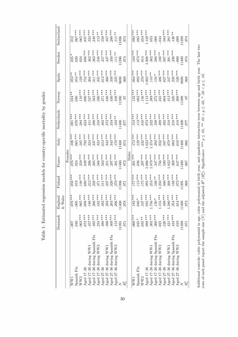
Tab

le1:

Est

imat

edre

gres

sion

mod

els

for

cou

ntr

y-s

pec

ific

mor

tali

tyby

gen

der

.

Den

mark

Engla

nd

Fin

land

Fra

nce

Italy

Net

her

lands

Norw

aySpain

Sw

eden

Sw

itze

rland

&W

ale

s

Fem

ale

s

WW

1-.

007

.078

***

.058

***

.076

***

.106

***

.081

***

.044

**

.053

**

.035

*.0

12

Spanis

hF

lu.0

40

-.005

.019

.024

.065

***

.070

***

.030

.054

**

.020

.067

***

WW

2.0

63

***

.065

***

.148

***

.259

***

.185

***

.284

***

.110

***

.129

***

.024

.065

***

Aged

17–26

.672

***

.698

***

.680

***

.839

***

.792

***

.624

***

.690

***

.752

***

.688

***

.837

***

Aged

17–26

duri

ng

WW

1.4

57

***

.186

***

.212

***

.206

***

.324

***

.411

***

.527

***

.304

***

.462

***

.324

***

Aged

17–26

duri

ng

Spanis

hF

lu.4

95

***

.266

***

.228

***

.305

***

.337

***

.398

***

.563

***

.311

***

.363

***

.248

***

Aged

17–26

duri

ng

WW

2.2

34

***

.442

***

.471

***

.566

***

.324

***

.318

***

.330

***

.335

***

.248

***

.113

**

Aged

27–36

.488

***

.482

***

.511

***

.562

***

.613

***

.482

***

.471

***

.612

***

.457

***

.558

***

Aged

27–36

duri

ng

WW

1.3

96

***

.203

***

.237

***

.251

***

.343

***

.372

***

.446

***

.360

***

.427

***

.357

***

Aged

27–36

duri

ng

Spanis

hF

lu.4

69

***

.263

***

.320

***

.297

***

.343

***

.334

***

.430

***

.339

***

.350

***

.288

***

Aged

27–36

duri

ng

WW

2.1

53

***

.206

***

.279

***

.381

***

.170

***

.103

**

.168

***

.235

***

.111

**

.111

**

N11391

11400

11396

11400

11400

11400

11390

9690

11396

11396

R2 a

.971

.978

.971

.972

.974

.977

.97

.969

.974

.974

Male

s

WW

1.0

60

***

.182

***

.177

***

.201

***

.172

***

.153

***

.122

***

.064

***

.103

***

.092

***

Spanis

hF

lu.0

45

*.0

40

*.1

13

***

.036

.129

***

.113

***

.082

***

.093

***

.073

***

.085

***

WW

2.0

35

**

.107

***

.175

***

.297

***

.232

***

.310

***

.156

***

.270

***

.014

.054

***

Aged

17–26

.988

***

.945

***

.985

***

1.0

86

***

1.0

23

***

.973

***

1.1

13

***

1.0

03

***

1.0

08

***

1.1

29

***

Aged

17–26

duri

ng

WW

1.3

05

***

1.7

56

***

.253

***

1.8

79

***

1.3

74

***

.232

***

.389

***

.110

**

.362

***

.053

Aged

17–26

duri

ng

Spanis

hF

lu.3

60

***

.130

*.1

66

**

.347

***

.292

***

.168

***

.272

***

.134

*.2

86

***

-.068

Aged

17–26

duri

ng

WW

2.0

25

1.1

55

***

1.2

50

***

.756

***

.932

***

.489

***

.245

***

.486

***

.100

**

-.044

Aged

27–36

.526

***

.499

***

.566

***

.599

***

.587

***

.492

***

.604

***

.627

***

.567

***

.583

***

Aged

27–36

duri

ng

WW

1.4

21

***

1.2

80

***

.268

***

1.8

22

***

.979

***

.318

***

.413

***

.247

***

.381

***

.281

***

Aged

27–36

duri

ng

Spanis

hF

lu.4

34

***

.354

***

.188

***

.369

***

.662

***

.218

***

.320

***

.220

***

.330

***

.136

**

Aged

27–36

duri

ng

WW

2.0

19

.654

***

.973

***

.647

***

.610

***

.418

***

.300

***

.526

***

-.000

-.009

N11399

11400

11395

11400

11400

11400

11398

9690

11400

11399

R2 a

.971

.973

.968

.967

.966

.977

.97

.968

.974

.974

Addit

ional

contr

ols

:cu

bic

poly

nom

ial

inage,

cubic

poly

nom

ial

inbir

thyea

r,and

quadra

tic

inte

ract

ion

term

bet

wee

nage

and

bir

thyea

r.T

he

last

two

row

sof

each

panel

rep

ort

the

sam

ple

size

(N)

and

the

adju

sted

R2

(R2 a).

Sig

nifi

cance

:***p≤

.01,

**.0

1<

p≤

.05,

*.0

5<

p≤

.10.

30

Table 2: Average residuals from model (1) at ages 50–59 by country and birth year.

Birth year1900–13 1914–18 1919–21 1922–35 1936–39 1940–45 1946–48

Females

Denmark -.248 -.130 -.051 .077 .087 .035 -.064England & Wales -.177 -.021 .056 .076 -.022 -.045 -.092Finland -.157 -.076 -.034 -.074 .005 .018 .058France -.154 -.071 -.029 -.031 -.040 -.029 -.007Italy -.166 -.041 -.002 .019 .006 .007 .015Netherlands -.197 -.084 -.054 -.030 -.012 .020 .022Norway -.204 -.103 -.032 .070 .089 .097 .104Spain -.200 -.080 -.028 -.072 -.058 -.055 -.074Sweden -.184 -.114 -.039 .002 .042 .076 .042Switzerland -.115 -.077 -.038 -.035 -.013 .053 .026

Males

Denmark -.093 -.065 .014 .035 -.068 -.139 -.238England & Wales -.034 .035 .071 .026 -.119 -.168 -.248Finland -.102 .025 .018 -.036 -.148 -.196 -.144France -.100 -.091 -.038 .000 -.095 -.140 -.136Italy -.046 .009 .067 .090 -.080 -.131 -.204Netherlands -.019 .103 .101 .035 -.079 -.115 -.170Norway -.099 .049 .076 .110 -.015 -.147 -.159Spain -.182 -.117 -.065 -.061 -.068 -.077 -.115Sweden -.161 -.056 .017 .055 -.058 -.121 -.170Switzerland -.058 -.052 -.045 -.047 -.128 -.140 -.168

31

Table 3: Percentage of respondents with absent father or mother at the age of 10, by period.

1935–38 1939–42 1943–45 1946–49 1950–55 1956–65

Father absent

Austria 19.15 22.58 27.87 27.43 21.35 13.72Belgium 5.59 5.22 11.39 6.99 9.29 5.50Czech Rep 6.25 5.26 7.38 11.93 9.29 9.26Denmark 5.77 9.09 7.63 10.43 10.49 7.41England 8.35 16.80 17.29 10.76 11.39 7.83France 11.56 12.92 18.35 16.99 13.78 6.30Germany 11.76 10.34 23.53 27.27 28.54 9.55Greece 1.54 1.72 2.73 3.79 4.70 1.60Italy 3.42 12.20 9.14 6.69 6.58 5.17Netherlands 8.24 6.67 10.22 10.45 7.80 4.55Poland 10.00 7.58 15.15 18.64 16.01 7.24Spain 12.90 11.86 11.17 16.58 7.52 5.44Sweden 11.11 11.02 12.21 10.18 13.41 11.62Switzerland 7.79 8.26 5.26 10.64 7.51 4.30

Mother absent

Austria 4.26 12.90 8.20 4.42 6.18 5.31Belgium 5.03 3.91 6.44 3.85 3.98 2.85Czech Rep .00 .75 1.64 2.27 3.18 3.09Denmark 3.85 5.30 5.93 3.07 3.58 2.51England 6.64 6.62 5.76 5.25 4.75 3.72France 6.80 5.62 6.33 7.77 6.22 3.15Germany 3.53 .86 3.36 5.93 3.03 2.87Greece 1.54 1.29 1.82 2.41 1.43 .44Italy 5.13 4.88 3.76 3.95 2.51 1.35Netherlands 1.18 2.96 4.38 2.27 3.07 1.91Poland 7.78 3.03 2.02 3.39 4.63 1.93Spain 9.68 4.64 7.98 7.49 3.62 3.74Sweden 1.71 7.63 6.87 3.98 4.71 5.28Switzerland 6.49 9.17 5.26 4.96 5.14 2.71

32

Table 4: SHARE: Least squares estimates of models for adult outcomes as function of hardshipexperienced in childhood or adolescence. Females.

Healthy FewChronic

War -.042 *** -.043 *** -.044 *** -.034 ** -.034 ** -.036 **Hunger -.053 ** -.030 -.026 -.050 ** -.032 -.023SES -.089 *** -.090 *** -.042 *** -.046 ***Chronic dis -.099 *** -.099 *** -.100 *** -.100 ***Father absent -.051 *** -.051 *** -.022 -.022Mother absent -.031 -.032 -.054 ** -.054 **War*SES .006 .021Hunger*SES -.018 -.036Constant .611 *** .643 *** .643 *** .576 *** .588 *** .588 ***N 10430 10263 10263 10424 10257 10257R2

a .095 .109 .109 .097 .103 .103

NotDepr EducYrs

War -.039 ** -.040 *** -.038 ** -.266 * -.359 *** -.349 ***Hunger -.114 *** -.096 *** -.087 *** -.699 *** -.330 * -.127SES -.054 *** -.047 *** -2.265 *** -2.195 ***Chronic dis -.133 *** -.132 *** .106 .104Father absent -.023 -.022 .286 ** .298 **Mother absent -.020 -.021 -.304 -.320War*SES -.018 -.104Hunger*SES -.032 -.753 **Constant .594 *** .613 *** .613 *** 8.106 *** 8.699 *** 8.708 ***N 10322 10155 10155 10400 10233 10233R2

a .068 .077 .077 .250 .323 .323

Numeracy Recall

War -.016 -.023 -.022 -.100 -.129 -.108Hunger -.036 * -.003 .001 -.105 .068 .165SES -.136 *** -.132 *** -.995 *** -.913 ***Chronic dis -.014 -.014 -.059 -.058Father absent -.035 ** -.034 ** -.017 -.009Mother absent .001 .000 .187 .175War*SES -.012 -.206 *Hunger*SES -.014 -.346Constant .263 *** .298 *** .299 *** 8.682 *** 8.910 *** 8.917 ***N 10407 10240 10240 10395 10229 10229R2

a .122 .145 .145 .209 .233 .233

LifeSat Happy

War -.126 ** -.128 ** -.111 * -.012 -.012 -.008Hunger -.402 *** -.297 *** -.294 *** -.080 *** -.057 ** -.072 ***SES -.346 *** -.295 *** -.067 *** -.060 ***Chronic dis -.294 *** -.292 *** -.070 *** -.070 ***Father absent -.179 *** -.176 *** -.044 ** -.044 **Mother absent -.024 -.029 .006 .006War*SES -.162 ** -.034 *Hunger*SES .006 .061Constant 7.348 *** 7.445 *** 7.448 *** .427 *** .444 *** .444 ***N 10367 10201 10201 10287 10123 10123R2

a .122 .134 .134 .049 .056 .056

Significance: *** p ≤ .01, ** .01 < p ≤ .05, * .05 < p ≤ .10. Standard errors are robust to heteroskedasticity.

33

Table 5: SHARE: Least squares estimates of models for adult outcomes as function of hardshipexperienced in childhood or adolescence. Males.

Healthy FewChronic

War -.031 * -.029 * -.027 -.020 -.020 -.019Hunger -.091 *** -.075 *** -.061 *** -.107 *** -.100 *** -.105 ***SES -.083 *** -.072 *** -.032 *** -.030 **Chronic dis -.037 * -.037 * -.075 *** -.075 ***Father absent -.019 -.018 -.009 -.009Mother absent .011 .010 -.030 -.030War*SES -.023 -.010Hunger*SES -.055 .021Constant .715 *** .730 *** .732 *** .676 *** .687 *** .687 ***N 8704 8547 8547 8702 8545 8545R2

a .077 .088 .088 .054 .057 .057

NotDepr EducYrs

War -.024 * -.023 * -.023 * -.346 ** -.345 ** -.290 *Hunger -.071 *** -.059 *** -.057 *** -.902 *** -.535 *** -.451 **SES -.046 *** -.044 *** -2.340 *** -2.145 ***Chronic dis -.066 *** -.066 *** .377 * .381 *Father absent -.021 -.021 .174 .177Mother absent .027 .027 -.458 * -.475 *War*SES -.005 -.538 ***Hunger*SES -.011 -.287Constant .800 *** .809 *** .809 *** 9.667 *** 1.168 *** 1.191 ***N 8599 8444 8444 8686 8529 8529R2

a .039 .045 .045 .195 .268 .269

Numeracy Recall

War -.033 * -.035 ** -.031 * -.178 -.219 * -.216 *Hunger -.038 * -.010 -.018 -.111 .037 .046SES -.144 *** -.133 *** -.857 *** -.846 ***Chronic dis -.015 -.014 -.165 -.165Father absent -.018 -.018 .092 .093Mother absent -.005 -.005 -.320 * -.321 *War*SES -.039 ** -.027Hunger*SES .037 -.035Constant .377 *** .413 *** .414 *** 8.322 *** 8.525 *** 8.527 ***N 8681 8525 8525 8645 8490 8490R2

a .117 .142 .143 .143 .165 .165

LifeSat Happy

War -.195 *** -.186 *** -.187 *** -.019 -.019 -.015Hunger -.181 ** -.143 * -.100 -.006 .008 .010SES -.242 *** -.229 *** -.061 *** -.049 ***Chronic dis -.157 ** -.157 ** -.006 -.005Father absent -.060 -.058 -.011 -.011Mother absent -.015 -.018 .020 .019War*SES -.006 -.034Hunger*SES -.182 -.004Constant 7.514 *** 7.572 *** 7.576 *** .446 *** .457 *** .458 ***N 8628 8472 8472 8562 8408 8408R2

a .086 .093 .093 .044 .047 .047

Significance: *** p ≤ .01, ** .01 < p ≤ .05, * .05 < p ≤ .10. Standard errors are robust to heteroskedasticity.

34

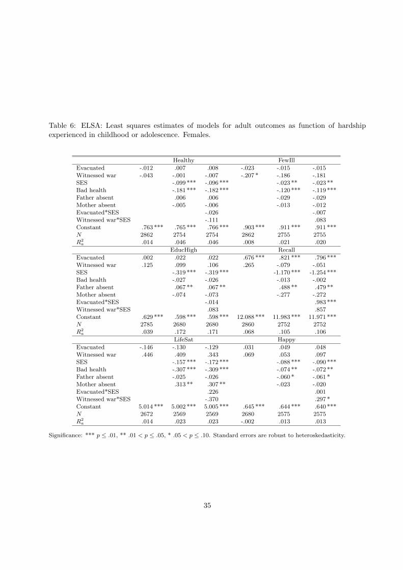
Table 6: ELSA: Least squares estimates of models for adult outcomes as function of hardshipexperienced in childhood or adolescence. Females.

Healthy FewIll

Evacuated -.012 .007 .008 -.023 -.015 -.015Witnessed war -.043 -.001 -.007 -.207 * -.186 -.181SES -.099 *** -.096 *** -.023 ** -.023 **Bad health -.181 *** -.182 *** -.120 *** -.119 ***Father absent .006 .006 -.029 -.029Mother absent -.005 -.006 -.013 -.012Evacuated*SES -.026 -.007Witnessed war*SES -.111 .083Constant .763 *** .765 *** .766 *** .903 *** .911 *** .911 ***N 2862 2754 2754 2862 2755 2755R2

a .014 .046 .046 .008 .021 .020

EducHigh Recall

Evacuated .002 .022 .022 .676 *** .821 *** .796 ***Witnessed war .125 .099 .106 .265 -.079 -.051SES -.319 *** -.319 *** -1.170 *** -1.254 ***Bad health -.027 -.026 -.013 -.002Father absent .067 ** .067 ** .488 ** .479 **Mother absent -.074 -.073 -.277 -.272Evacuated*SES -.014 .983 ***Witnessed war*SES .083 .857Constant .629 *** .598 *** .598 *** 12.088 *** 11.983 *** 11.971 ***N 2785 2680 2680 2860 2752 2752R2

a .039 .172 .171 .068 .105 .106

LifeSat Happy

Evacuated -.146 -.130 -.129 .031 .049 .048Witnessed war .446 .409 .343 .069 .053 .097SES -.157 *** -.172 *** -.088 *** -.090 ***Bad health -.307 *** -.309 *** -.074 ** -.072 **Father absent -.025 -.026 -.060 * -.061 *Mother absent .313 ** .307 ** -.023 -.020Evacuated*SES .226 .001Witnessed war*SES -.370 .297 *Constant 5.014 *** 5.002 *** 5.005 *** .645 *** .644 *** .640 ***N 2672 2569 2569 2680 2575 2575R2

a .014 .023 .023 -.002 .013 .013

Significance: *** p ≤ .01, ** .01 < p ≤ .05, * .05 < p ≤ .10. Standard errors are robust to heteroskedasticity.

35

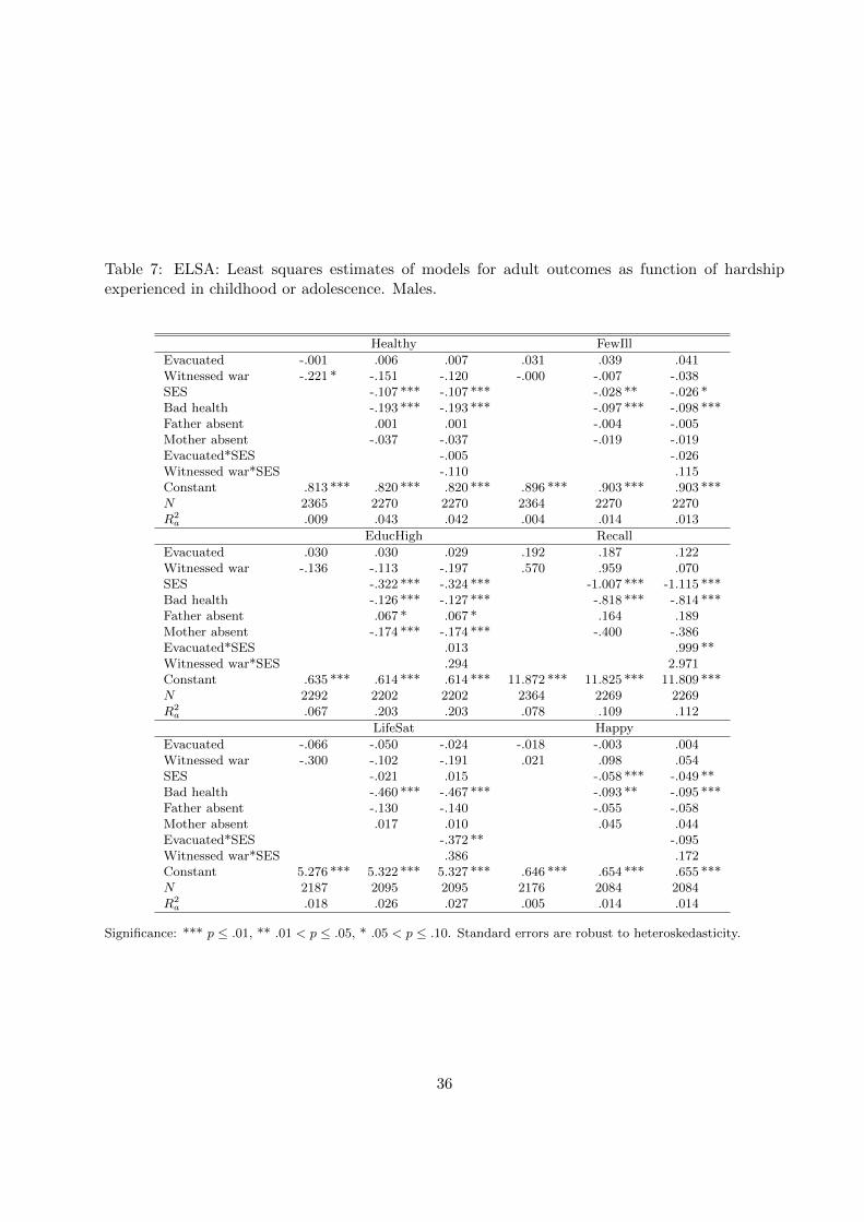
Table 7: ELSA: Least squares estimates of models for adult outcomes as function of hardshipexperienced in childhood or adolescence. Males.

Healthy FewIll

Evacuated -.001 .006 .007 .031 .039 .041Witnessed war -.221 * -.151 -.120 -.000 -.007 -.038SES -.107 *** -.107 *** -.028 ** -.026 *Bad health -.193 *** -.193 *** -.097 *** -.098 ***Father absent .001 .001 -.004 -.005Mother absent -.037 -.037 -.019 -.019Evacuated*SES -.005 -.026Witnessed war*SES -.110 .115Constant .813 *** .820 *** .820 *** .896 *** .903 *** .903 ***N 2365 2270 2270 2364 2270 2270R2

a .009 .043 .042 .004 .014 .013

EducHigh Recall

Evacuated .030 .030 .029 .192 .187 .122Witnessed war -.136 -.113 -.197 .570 .959 .070SES -.322 *** -.324 *** -1.007 *** -1.115 ***Bad health -.126 *** -.127 *** -.818 *** -.814 ***Father absent .067 * .067 * .164 .189Mother absent -.174 *** -.174 *** -.400 -.386Evacuated*SES .013 .999 **Witnessed war*SES .294 2.971Constant .635 *** .614 *** .614 *** 11.872 *** 11.825 *** 11.809 ***N 2292 2202 2202 2364 2269 2269R2

a .067 .203 .203 .078 .109 .112

LifeSat Happy

Evacuated -.066 -.050 -.024 -.018 -.003 .004Witnessed war -.300 -.102 -.191 .021 .098 .054SES -.021 .015 -.058 *** -.049 **Bad health -.460 *** -.467 *** -.093 ** -.095 ***Father absent -.130 -.140 -.055 -.058Mother absent .017 .010 .045 .044Evacuated*SES -.372 ** -.095Witnessed war*SES .386 .172Constant 5.276 *** 5.322 *** 5.327 *** .646 *** .654 *** .655 ***N 2187 2095 2095 2176 2084 2084R2

a .018 .026 .027 .005 .014 .014

Significance: *** p ≤ .01, ** .01 < p ≤ .05, * .05 < p ≤ .10. Standard errors are robust to heteroskedasticity.

36

Figure 1: Mortality contours.

(a) Females0

2040

6080

020

4060

80

190019201940196019802000 190019201940196019802000 190019201940196019802000

England and Wales France Italy

Netherlands Spain Sweden

Age

Year

(b) Males

020

4060

800

2040

6080

190019201940196019802000 190019201940196019802000 190019201940196019802000

England and Wales France Italy

Netherlands Spain Sweden

Age

Year

This figure presents the contours plots of gender-specific death rates by age during the period 1890–2009 forEngland and Wales, France, Italy, the Netherlands, Spain and Sweden (green ≤ .1 percent, light blue .2–.8 percent,blue .8–3.0 percent, purple 3–7 percent, red > 7 percent).

37

Figure 2: Hunger experience and hunger duration.

(a) Percent experiencing hunger0

1020

010

200

1020

010

20

1935 1945 1955 1965

Austria Belgium Czech Rep Denmark

France Germany Greece Italy

Netherlands Poland Spain Sweden

Switzerland

Per

cent

Year

(b) Distribution of the year when hunger started and ended

050

100

050

100

050

100

050

100

1935 1945 1955 1965

Austria Belgium Czech Rep Denmark

France Germany Greece Italy

Netherlands Poland Spain Sweden

Switzerland

Started Ended

Per

cent

Year

The top panel shows the percentage of people born in 1930–1956 who report experiencing hunger in each single yearduring the period 1935–65. The bottom panel shows the cumulative distribution function of the starting and endingyears of hunger episodes for all people who report a period of hunger before age 17. The red vertical bars mark theWW2 period (1939–45).

38

Figure 3: Geography of hunger and war.

20.0 - 50.017.5 - 20.015.0 - 17.512.5 - 15.010.0 - 12.57.5 - 10.05.0 - 7.52.5 - 5.00.0 - 2.5No data

20.0 - 50.017.5 - 20.015.0 - 17.512.5 - 15.010.0 - 12.57.5 - 10.05.0 - 7.52.5 - 5.00.0 - 2.5No data

No war

1 year

2 years

3 years or more

No data

This figure shows the regional distribution of hunger and war in Europe. The two top panels show the percentage ofrespondents having ever suffered hunger between age 5–16, separately for the cohorts born in 1930–39 (top-leftpanel) and 1940–49 (top-right panel). The shading in the map becomes darker when the percentage of peoplereporting hunger ranges between 20 and 50%. The bottom panel shows the number of years of potential exposure towar for exactly the same regions during the period from the beginning of the Spanish Civil War in 1936 to the endof WW2 in 1945. The shading in the map becomes darker as the number of years of potential exposure to warincreases (the darkest color corresponds to 3 years of war or more).

39

A Details on SHARE and ELSA

This appendix provides some detail on the temporal and spatial information provided by SHARE

and ELSA, and the information on childhood health and SES, hardship episodes in childhood, and

adult outcomes.

A.1 Temporal and spatial information

A key feature of the public use version of SHARELIFE is the possibility of determining the country,

region and area in which an individual was living in any given year. The basic information comes

from Module AC (Accommodation), which collects information on the different places an individual

lived in during her life. The module begins with a question on the residence the respondent lived

in when was born, where by residence is meant an apartment or single house. It then collects

information on each other residence the respondent lived in for more than 6 months, including the

year the person started and stopped living at that residence, the country (at current boundaries),

the region (at different level of geographically detail depending on the country) and the area of

residence (big city, suburbs or outskirts of a big city, large town, small town, rural area or village).

Regarding the country of residence, two questions are asked. First, for each past residence the

survey instrument asks whether it was within the current boundaries of the country in which the

respondent is currently living. If the answer is no, a second question is asked using a showcard:

Which country, considering current boundaries, was this residence in? The showcard reports the

names of the main European countries, Russia, the USA, and two residual categories, namely other

European country and other non-European country. The region of residence is asked only if the

country of past residence coincides with that of current residence. This means that the region

of residence cannot be determined for those who in a given year have changed their country of

residence.

Since we know the starting and ending year and the country/region/area of each residency, we

are able to construct a longitudinal data set with annual observations for each individual. Although

SHARELIFE adopts the Nomenclature of Units for Territorial Statistics (NUTS) developed by the

European Union, the level of regional disaggregation varies by country: it is at the coarse NUTS1

level for Belgium, Denmark, France and the Netherlands, at the fine NUTS3 level for the Czech

Republic, and at the intermediate but not very detailed NUTS2 level for Austria, Germany, Greece,

Italy, Poland, Spain, Sweden and Switzerland.

Unlike SHARELIFE, the public use version of ELSALIFE contains little information on past

40

residence and no information that can be used to determine the country and region of residence in

a given year. Basically, we can only determine whether the respondent was living in the U.K. or

abroad in a given year.

A.2 SES and health in childhood

Module CS (Childhood SES) of SHARELIFE collects information on the occupation of the main

breadwinner (white collar, blue collar, farmer, etc.), the number of books at home, features of

the accommodation (presence of fixed bath, running water, inside toilet, central heating, number

of rooms available), the number of people living in the house when the respondent was aged 10,

and whether parents, siblings and grandparents were living in the house when the respondent was

aged 10. Module HS (Health status) of SHARELIFE contains information on both the self-rated

health status in childhood (age 0–15) as well as experiences of distinct illnesses during childhood

(infectious diseases, polio, asthma, allergies, heart trouble, etc.). Then, for each illness, it is asked

the age-interval when it was experienced: between age 0–5, 6–10, 11–15. We construct a measure

of childhood health that counts the number of chronic illnesses respondents experienced in the

age interval 6–15, considering the following diseases: polio, asthma, allergies (other than asthma),

epilepsy, psychiatric problems, diabetes, heart trouble, leukaemia or lymphoma and cancer.

ELSALIFE asks comparable questions regarding the number of books at home, features of

the accommodation, the presence of distinct members of the family (all measured with reference

to age 10) and health status in childhood. However, there are some differences with respect to

SHARELIFE. In particular, ELSALIFE does not collect information on the occupation of the main

breadwinner when the respondent was aged 10, but rather on the occupation of the father when

the respondent was aged 14. Further, it does not include questions on the specific timing of the

illnesses experienced during childhood. For health status in childhood we use a binary indicator

for being in fair or poor health based on the self-rated health measure.

A.3 Hardship episodes in childhood

Module GL (General Life) of SHARELIFE collects information on the experience of hardship

episodes. This section first asks: Looking back on your life, was there a distinct period during

which you were under more stress compared to the rest of your life? If the answer is yes, it asks

When did this period start?, followed by When did this period stop? It then asks similar questions

for poor health (Looking back on your life, was there a distinct period during which your health

was poor compared to the rest of your life?), financial hardship (Looking back on your life, was

41

there a distinct period of financial hardship?), and hunger (Looking back on your life, was there a

distinct period during which you suffered from hunger?). The formulation of these questions allows

to determine the duration of the reported hardship episode, defined as the difference between the

year when they ended and the year when they started, although we have no other information

on their intensity. Notice that respondents are asked to report only one episode for each type of

hardship, presumably the most salient (phrases such as “distinct period” or “compared to the rest

of your life” are meant to capture this idea). Also notice that there may be heterogeneity in the

perception of each hardship across individuals, which raises the issue of interpersonal comparability.

Unlike SHARELIFE, ELSALIFE gathers direct information on having witnessed serious injury

or death of someone in war or military action, and having been evacuated during WW2. Specifically,

the survey instrument asks: Have you ever witnessed the serious injury or death of someone in war

or military action? If the answer is yes, it then asks: How old were you when it first happened?

The next question is directly about WW2: Have you ever been evacuated during World War II?

Like SHARELIFE, ELSALIFE also gathers information on having experienced severe financial

hardship and on the family’s SES around age 10. Specifically, the survey instrument asks: Have

you ever experienced severe financial hardship?. If the answer is yes, the interviewee is then asked:

How old were you when it first happened?.

The questions about the family’s SES around age 10 are very similar in both surveys. They

include the number of books at home, accommodation features, the job of the main breadwinner,

and whether distinct members of the family were present in the house when aged 10. The latter

question is used to infer information on the absence of the father and the mother. Notice that

financial hardship and absence of the father when aged 10 are the only hardship episodes directly

comparable with those recorded in SHARE. Further, we only know the age when financial hardship

started, not its duration. This means that we can only estimate the long-term effects of financial

hardship episodes that started at a given age, not of financial hardship experienced at different

ages.

A.4 Adult outcomes

The adult outcomes that we consider are all collected in the regular waves of SHARE and ELSA.

Some of these outcomes are directly comparable between the two surveys, but others are not.

The comparable outcomes are SRH, the test of memory (recall), life satisfaction and happiness.

SRH is defined on a 1–5 scale for both surveys with a slight difference in the definition of the

42

categories (for SHARE the available categories are “excellent”, “very good”, “good”, “fair”, “poor”,

whereas for ELSA the available categories are “very good”, “good”, “fair”, “bad” and “very bad”).

For both SHARE and ELSA, the memory test consists of verbal registration and recall of a list of

10 words, carried out twice, first immediately after the encoding phase (immediate recall) and then

some 5 minutes later (delayed recall). Our measure of recall is the sum of the scores on immediate

and delayed recall, which ranges from a minimum of 0 to a maximum of 20. The numeracy test

in SHARE consists of five questions involving simple arithmetical calculations based on real life

situations and the test score ranges from a minimum of 1 to a maximum of 5. In ELSA, instead,

the numeracy test was only administered in wave 1.

The precise wording of the question on life satisfaction and its scale are different for the two

surveys. SHARE respondents are asked to choose a value between 0 and 10, with 0 meaning

“completely dissatisfied” and 10 meaning “completely dissatisfied”, while ELSA respondents are

asked to choose a value between 1 and 7, with 1 meaning “strongly agree” and 7 meaning “strongly

disagree”. Happiness is instead defined in the same way in both surveys.

Important differences between SHARE and ELSA arise for BMI, education and depression. In

SHARE, BMI is computed from self reported height and weight, while in ELSA it is computed

from objective measured taken during the nurse visit. Unlike SHARE, ELSA does not ask the

number of years of completed schooling but asks instead the age at which the respondent left full

time education. Finally, as a measure of mental health SHARE uses the Euro-D index, which

considers several dimensions (depression, anxiety, suicidality, etc.), while ELSA only asks whether

the respondent was feeling depressed in the past week.

A.5 Nonsampling errors

Like most household surveys, both SHARE and ELSA suffer of sample attrition and item nonre-

sponse. In addition, the life-history data collected in the two surveys may be affected by recall

bias, coloring, and limited information on certain variables.

Despite the adoption of preventive procedures, such as training of the interviewers and survey

design characteristics, sample attrition is an important feature of both surveys. For example,

Schroder (2008) shows that the attrition rate between wave 1 and wave 2 of SHARE is about 28%

(net of the people who died between the two waves), but varies considerably by country ranging

from a minimum of 13% in Greece to a maximum of 41% in Germany. On the other hand, he finds

no significant differences in attrition rates by gender.

43

Item nonresponse arises when individuals do not answer a particular question. In both surveys,

nonresponse is important for income and wealth, but is unimportant for health, hardships and

childhood circumstances.

Recall error arises when respondents do not remember precisely when and how an event took

place in the past. There are concerns that the problem may be especially important when the

population of interest consists of elderly people. In fact, Havari and Mazzonna (2015) find little

evidence of this kind of error. Their evidence may reflects a distinctive advantage of SHARELIFE

and ELSALIFE over other surveys, namely that both apply the life-history calendar method, which

is based on temporal landmarks (events that are striking or easier to remember) and therefore likely

to be more accurate (see for example Groves et al. 2004).

Even when an event is a temporal landmark, one cannot rule out coloring, namely the fact that

respondents may answer questions about the distant past based on post-event information, such as

their current status or macro-events that are part of a country’s narrative. We find little evidence

of coloring in SHARE and ELSA when using information on hardships.

44

B Additional tables and graphs

45

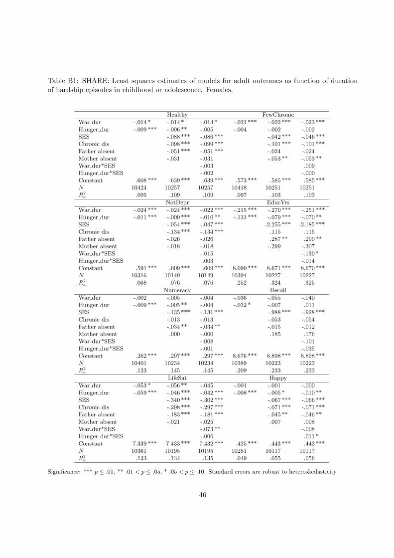
Table B1: SHARE: Least squares estimates of models for adult outcomes as function of durationof hardship episodes in childhood or adolescence. Females.

Healthy FewChronic

War dur -.014 * -.014 * -.014 * -.021 *** -.022 *** -.023 ***Hunger dur -.009 *** -.006 ** -.005 -.004 -.002 -.002SES -.088 *** -.086 *** -.042 *** -.046 ***Chronic dis -.098 *** -.099 *** -.101 *** -.101 ***Father absent -.051 *** -.051 *** -.024 -.024Mother absent -.031 -.031 -.053 ** -.053 **War dur*SES -.003 .009Hunger dur*SES -.002 -.000Constant .608 *** .639 *** .639 *** .573 *** .585 *** .585 ***N 10424 10257 10257 10418 10251 10251R2

a .095 .109 .109 .097 .103 .103

NotDepr EducYrs

War dur -.024 *** -.024 *** -.022 *** -.215 *** -.270 *** -.251 ***Hunger dur -.011 *** -.009 *** -.010 ** -.131 *** -.079 *** -.070 **SES -.054 *** -.047 *** -2.255 *** -2.185 ***Chronic dis -.134 *** -.134 *** .115 .115Father absent -.026 -.026 .287 ** .290 **Mother absent -.018 -.018 -.299 -.307War dur*SES -.015 -.130 *Hunger dur*SES .003 -.014Constant .591 *** .609 *** .609 *** 8.090 *** 8.671 *** 8.670 ***N 10316 10149 10149 10394 10227 10227R2

a .068 .076 .076 .252 .324 .325

Numeracy Recall

War dur -.002 -.005 -.004 -.036 -.055 -.040Hunger dur -.009 *** -.005 ** -.004 -.032 * -.007 .011SES -.135 *** -.131 *** -.988 *** -.928 ***Chronic dis -.013 -.013 -.053 -.054Father absent -.034 ** -.034 ** -.015 -.012Mother absent .000 -.000 .185 .176War dur*SES -.008 -.101Hunger dur*SES -.001 -.035Constant .262 *** .297 *** .297 *** 8.676 *** 8.898 *** 8.898 ***N 10401 10234 10234 10389 10223 10223R2

a .123 .145 .145 .209 .233 .233

LifeSat Happy

War dur -.053 * -.056 ** -.045 -.001 -.001 -.000Hunger dur -.059 *** -.046 *** -.042 *** -.008 *** -.005 * -.010 **SES -.340 *** -.302 *** -.067 *** -.066 ***Chronic dis -.298 *** -.297 *** -.071 *** -.071 ***Father absent -.183 *** -.181 *** -.045 ** -.046 **Mother absent -.021 -.025 .007 .008War dur*SES -.073 ** -.008Hunger dur*SES -.006 .011 *Constant 7.339 *** 7.433 *** 7.432 *** .425 *** .443 *** .443 ***N 10361 10195 10195 10281 10117 10117R2

a .123 .134 .135 .049 .055 .056

Significance: *** p ≤ .01, ** .01 < p ≤ .05, * .05 < p ≤ .10. Standard errors are robust to heteroskedasticity.

46

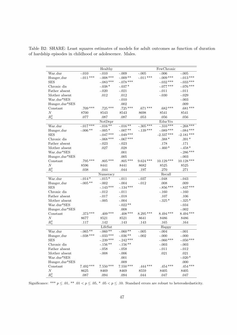
Table B2: SHARE: Least squares estimates of models for adult outcomes as function of durationof hardship episodes in childhood or adolescence. Males.

Healthy FewChronic

War dur -.010 -.010 -.009 -.005 -.006 -.005Hunger dur -.011 *** -.008 *** -.009 ** -.011 *** -.009 *** -.013 ***SES -.083 *** -.078 *** -.032 *** -.033 ***Chronic dis -.038 * -.037 * -.077 *** -.076 ***Father absent -.020 -.021 -.011 -.011Mother absent .012 .012 -.030 -.029War dur*SES -.010 -.003Hunger dur*SES .002 .009Constant .709 *** .725 *** .725 *** .671 *** .682 *** .681 ***N 8700 8543 8543 8698 8541 8541R2

a .077 .087 .087 .053 .056 .056

NotDepr EducYrs

War dur -.017 *** -.016 ** -.016 ** -.305 *** -.310 *** -.268 ***Hunger dur -.006 ** -.005 * -.007 ** -.139 *** -.089 *** -.084 ***SES -.047 *** -.049 *** -2.337 *** -2.181 ***Chronic dis -.068 *** -.067 *** .388 * .391 *Father absent -.023 -.023 .178 .171Mother absent .027 .028 -.460 * -.458 *War dur*SES .001 -.286 ***Hunger dur*SES .005 -.003Constant .795 *** .805 *** .805 *** 9.624 *** 10.129 *** 10.128 ***N 8596 8441 8441 8682 8525 8525R2

a .038 .044 .044 .197 .270 .271

Numeracy Recall

War dur -.014 * -.015 * -.011 -.037 -.048 -.043Hunger dur -.005 ** -.002 -.004 -.012 .008 .009SES -.143 *** -.134 *** -.856 *** -.837 ***Chronic dis -.012 -.011 -.160 -.160Father absent -.017 -.018 .107 .106Mother absent -.005 -.004 -.325 * -.325 *War dur*SES -.022 ** -.034Hunger dur*SES .008 -.002Constant .373 *** .409 *** .408 *** 8.295 *** 8.494 *** 8.494 ***N 8677 8521 8521 8641 8486 8486R2

a .117 .142 .143 .143 .165 .164

LifeSat Happy

War dur -.065 ** -.060 ** -.060 ** -.005 -.004 -.001Hunger dur -.038 *** -.033 *** -.036 ** -.002 -.000 -.000SES -.239 *** -.242 *** -.060 *** -.050 ***Chronic dis -.156 ** -.156 ** -.003 -.003Father absent -.058 -.058 -.011 -.012Mother absent -.008 -.006 .021 .021War dur*SES .001 -.020 *Hunger dur*SES .009 .000Constant 7.492 *** 7.550 *** 7.550 *** .444 *** .454 *** .454 ***N 8625 8469 8469 8559 8405 8405R2

a .087 .094 .094 .044 .047 .047

Significance: *** p ≤ .01, ** .01 < p ≤ .05, * .05 < p ≤ .10. Standard errors are robust to heteroskedasticity.

47

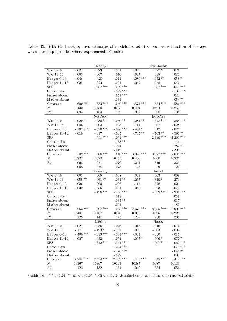
Table B3: SHARE: Least squares estimates of models for adult outcomes as function of the agewhen hardship episodes where experienced. Females.

Healthy FewChronic

War 0–10 -.021 -.023 -.021 -.026 -.027 * -.026War 11–16 -.003 -.007 -.010 .027 .025 .031Hunger 0–10 -.046 -.028 -.014 -.080 *** -.072 ** -.058 *Hunger 11–16 -.025 -.023 -.034 .052 .052 .049SES -.087 *** -.089 *** -.037 *** -.041 ***Chronic dis -.099 *** -.101 ***Father absent -.051 *** -.022Mother absent -.031 -.054 **Constant .609 *** .633 *** .640 *** .574 *** .584 *** .586 ***N 10430 10430 10263 10424 10424 10257R2

a .094 .104 .109 .097 .098 .103

NotDepr EducYrs

War 0–10 -.029 ** -.030 ** -.030 ** -.284 ** -.348 *** -.368 ***War 11–16 .006 .003 .005 .111 .007 -.028Hunger 0–10 -.107 *** -.096 *** -.096 *** -.431 * .012 -.077Hunger 11–16 -.019 -.017 -.005 -.745 ** -.703 ** -.591 **SES -.051 *** -.054 *** -2.140 *** -2.263 ***Chronic dis -.133 *** .113Father absent -.024 .282 **Mother absent -.019 -.302Constant .592 *** .606 *** .610 *** 8.095 *** 8.677 *** 8.683 ***N 10322 10322 10155 10400 10400 10233R2

a .068 .071 .076 .251 .319 .323.068 .078 .078 .25 .29 .29

Numeracy Recall

War 0–10 -.001 -.005 -.008 .023 -.003 -.008War 11–16 -.055 ** -.061 ** -.061 ** -.267 -.310 * -.273Hunger 0–10 -.026 -.000 .006 -.115 .078 .021Hunger 11–16 -.039 -.036 -.031 -.042 -.023 .075SES -.126 *** -.136 *** -.939 *** -.995 ***Chronic dis -.013 -.059Father absent -.035 ** -.017Mother absent .001 .187Constant .263 *** .297 *** .298 *** 8.679 *** 8.935 *** 8.904 ***N 10407 10407 10240 10395 10395 10229R2

a .123 .141 .145 .209 .230 .233

LifeSat Happy

War 0–10 -.027 -.036 -.026 -.015 -.016 -.014War 11–16 -.177 -.193 * -.167 .000 -.003 -.004Hunger 0–10 -.460 *** -.393 *** -.334 *** -.044 -.030 -.015Hunger 11–16 -.037 -.032 -.051 -.067 * -.066 * -.070 *SES -.322 *** -.344 *** -.067 *** -.067 ***Chronic dis -.294 *** -.070 ***Father absent -.178 *** -.045 **Mother absent -.022 .007Constant 7.344 *** 7.434 *** 7.439 *** .426 *** .445 *** .444 ***N 10367 10367 10201 10287 10287 10123R2

a .122 .132 .134 .049 .054 .056

Significance: *** p ≤ .01, ** .01 < p ≤ .05, * .05 < p ≤ .10. Standard errors are robust to heteroskedasticity.

48

Table B4: SHARE: Least squares estimates of models for adult outcomes as function of the agewhen hardship episodes where experienced. Males.

Healthy FewChronic

War 0–10 -.022 -.023 -.021 -.023 -.023 -.021War 11–16 -.004 -.005 -.003 .031 .030 .030Hunger 0–10 -.048 * -.038 -.034 -.099 *** -.096 *** -.092 ***Hunger 11–16 -.065 * -.060 * -.057 -.019 -.018 -.019SES -.078 *** -.083 *** -.027 *** -.032 ***Chronic dis -.037 * -.076 ***Father absent -.019 -.009Mother absent .011 -.029Constant .711 *** .731 *** .727 *** .674 *** .680 *** .684 ***N 8704 8704 8547 8702 8702 8545R2

a .076 .085 .087 .054 .055 .057

NotDepr EducYrs

War 0–10 -.018 -.018 -.018 -.347 ** -.373 *** -.333 **War 11–16 -.010 -.011 -.003 .093 .052 -.022Hunger 0–10 -.019 -.013 -.006 -.822 *** -.536 ** -.553 **Hunger 11–16 -.069 ** -.066 ** -.068 ** -.549 ** -.407 -.330SES -.044 *** -.046 *** -2.192 *** -2.336 ***Chronic dis -.066 *** .383 *Father absent -.022 .184Mother absent .027 -.449 *Constant .797 *** .808 *** .806 *** 9.643 *** 1.201 *** 1.147 ***N 8599 8599 8444 8686 8686 8529R2

a .038 .042 .044 .196 .259 .269

Numeracy Recall

War 0–10 -.035 ** -.036 ** -.036 ** -.163 -.172 * -.198 *War 11–16 -.034 -.037 -.043 .077 .061 .021Hunger 0–10 -.044 -.026 -.022 -.107 -.001 .016Hunger 11–16 -.018 -.010 -.004 -.002 .048 .058SES -.133 *** -.143 *** -.800 *** -.858 ***Chronic dis -.014 -.167Father absent -.017 .092Mother absent -.005 -.313 *Constant .377 *** .411 *** .413 *** 8.306 *** 8.508 *** 8.508 ***N 8681 8681 8525 8645 8645 8490R2

a .118 .138 .143 .143 .161 .165

LifeSat Happy

War 0–10 -.168 *** -.170 *** -.159 *** -.032 * -.033 * -.032 *War 11–16 .021 .019 .038 .045 .044 .039Hunger 0–10 -.047 -.017 -.006 -.017 -.008 -.005Hunger 11–16 -.264 ** -.251 * -.254 * .023 .026 .028SES -.224 *** -.242 *** -.061 *** -.061 ***Chronic dis -.155 ** -.006Father absent -.061 -.011Mother absent -.010 .022Constant 7.497 *** 7.553 *** 7.555 *** .444 *** .459 *** .455 ***N 8628 8628 8472 8562 8562 8408R2

a .086 .092 .093 .045 .049 .048

Significance: *** p ≤ .01, ** .01 < p ≤ .05, * .05 < p ≤ .10. Standard errors are robust to heteroskedasticity.

49

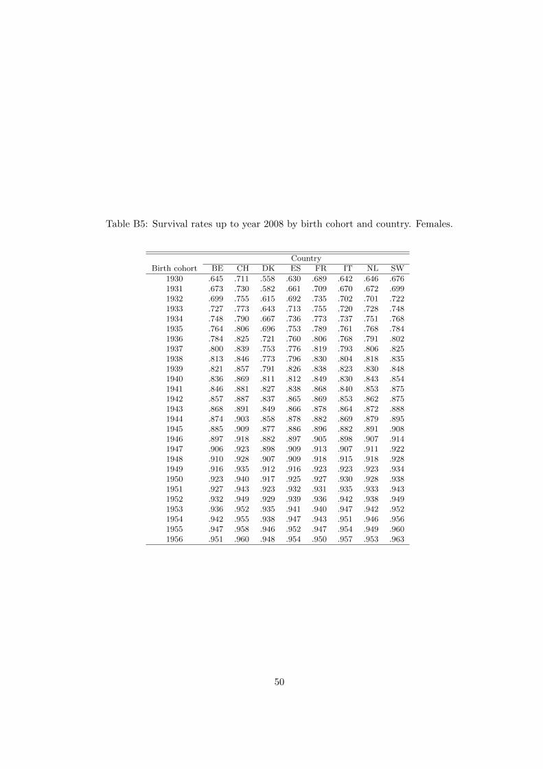
Table B5: Survival rates up to year 2008 by birth cohort and country. Females.

CountryBirth cohort BE CH DK ES FR IT NL SW

1930 .645 .711 .558 .630 .689 .642 .646 .6761931 .673 .730 .582 .661 .709 .670 .672 .6991932 .699 .755 .615 .692 .735 .702 .701 .7221933 .727 .773 .643 .713 .755 .720 .728 .7481934 .748 .790 .667 .736 .773 .737 .751 .7681935 .764 .806 .696 .753 .789 .761 .768 .7841936 .784 .825 .721 .760 .806 .768 .791 .8021937 .800 .839 .753 .776 .819 .793 .806 .8251938 .813 .846 .773 .796 .830 .804 .818 .8351939 .821 .857 .791 .826 .838 .823 .830 .8481940 .836 .869 .811 .812 .849 .830 .843 .8541941 .846 .881 .827 .838 .868 .840 .853 .8751942 .857 .887 .837 .865 .869 .853 .862 .8751943 .868 .891 .849 .866 .878 .864 .872 .8881944 .874 .903 .858 .878 .882 .869 .879 .8951945 .885 .909 .877 .886 .896 .882 .891 .9081946 .897 .918 .882 .897 .905 .898 .907 .9141947 .906 .923 .898 .909 .913 .907 .911 .9221948 .910 .928 .907 .909 .918 .915 .918 .9281949 .916 .935 .912 .916 .923 .923 .923 .9341950 .923 .940 .917 .925 .927 .930 .928 .9381951 .927 .943 .923 .932 .931 .935 .933 .9431952 .932 .949 .929 .939 .936 .942 .938 .9491953 .936 .952 .935 .941 .940 .947 .942 .9521954 .942 .955 .938 .947 .943 .951 .946 .9561955 .947 .958 .946 .952 .947 .954 .949 .9601956 .951 .960 .948 .954 .950 .957 .953 .963

50

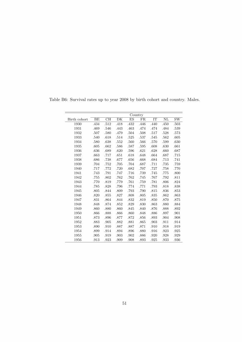
Table B6: Survival rates up to year 2008 by birth cohort and country. Males.

CountryBirth cohort BE CH DK ES FR IT NL SW

1930 .434 .512 .418 .432 .446 .440 .450 .5031931 .469 .546 .443 .463 .474 .474 .484 .5391932 .507 .580 .479 .504 .508 .517 .528 .5731933 .540 .618 .514 .525 .537 .545 .562 .6051934 .580 .638 .552 .560 .566 .570 .599 .6301935 .605 .662 .586 .587 .595 .608 .630 .6611936 .636 .689 .620 .596 .621 .628 .660 .6871937 .663 .717 .651 .618 .648 .664 .687 .7151938 .686 .738 .677 .656 .668 .684 .713 .7411939 .704 .752 .705 .704 .687 .711 .735 .7591940 .717 .772 .720 .682 .707 .727 .758 .7701941 .743 .791 .747 .716 .739 .745 .775 .8001942 .755 .802 .762 .762 .745 .767 .792 .8111943 .770 .819 .779 .761 .759 .781 .806 .8241944 .785 .828 .796 .774 .771 .793 .818 .8381945 .805 .844 .809 .793 .790 .815 .836 .8531946 .820 .855 .827 .808 .805 .835 .862 .8631947 .831 .864 .844 .832 .819 .850 .870 .8751948 .848 .874 .852 .829 .830 .863 .880 .8841949 .860 .880 .860 .845 .840 .876 .888 .8921950 .866 .888 .866 .860 .848 .886 .897 .9011951 .873 .896 .877 .872 .856 .893 .904 .9081952 .883 .905 .882 .881 .865 .903 .911 .9141953 .890 .910 .887 .887 .871 .910 .918 .9191954 .899 .914 .894 .896 .880 .916 .923 .9251955 .905 .919 .903 .902 .886 .920 .928 .9291956 .913 .923 .909 .908 .893 .925 .933 .936

51

Figure B1: Stress experience and stress duration

(a) Percent reporting stress0

12

30

12

30

12

30

12

3

1935 1945 1955 1965

Austria Belgium Czech Rep Denmark

France Germany Greece Italy

Netherlands Poland Spain Sweden

Switzerland

Per

cent

Year

(b) Distribution of the year when stress started and ended

050

100

050

100

050

100

050

100

1935 1945 1955 1965

Austria Belgium Czech Rep Denmark

France Germany Greece Italy

Netherlands Poland Spain Sweden

Switzerland

Started Ended

Per

cent

Year

The top panel shows the percentage of people born in 1930–1956 who report experiencing stress in each single yearduring the period 1935–65. The bottom panel shows the cumulative distribution function of the starting and endingyears of stress episodes for all people who report a period of stress before age 17. The red vertical bars mark theWW2 period (1939–45).

52

Figure B2: Financial hardship experience and duration

(a) Percent reporting financial hardship0

24

68

02

46

80

24

68

02

46

8

1935 1945 1955 1965

Austria Belgium Czech Rep Denmark

France Germany Greece Italy

Netherlands Poland Spain Sweden

Switzerland

Per

cent

Year

(b) Distribution of the year when financial hardship started and ended

050

100

050

100

050

100

050

100

1935 1945 1955 1965

Austria Belgium Czech Rep Denmark

France Germany Greece Italy

Netherlands Poland Spain Sweden

Switzerland

Started Ended

Per

cent

Year

The top panel shows the percentage of people born in 1930–1956 who report experiencing financial hardship in eachsingle year during the period 1935–65. The bottom panel shows the cumulative distribution function of the startingand ending years of financial hardship episodes for all people who report a period of financial hardship beforeage 17. The red vertical bars mark the WW2 period (1939–45).

53

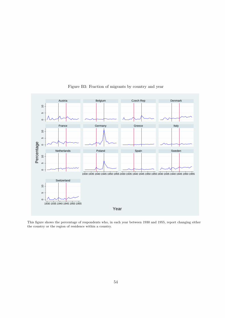
Figure B3: Fraction of migrants by country and year

05

100

510

05

100

510

1930 1935 1940 1945 1950 1955 1930 1935 1940 1945 1950 1955 1930 1935 1940 1945 1950 1955

1930 1935 1940 1945 1950 1955

Austria Belgium Czech Rep Denmark

France Germany Greece Italy

Netherlands Poland Spain Sweden

Switzerland

Per

cent

age

Year

This figure shows the percentage of respondents who, in each year between 1930 and 1955, report changing eitherthe country or the region of residence within a country.

54