Growing Pains: The School Consolidation Movement and Student Outcomes

Christopher Berry

Harris School of Public Policy The University of Chicago

crberry@uchicago.edu

Martin West Department of Government

Program on Education Policy and Governance Harvard University

mrwest@fas.harvard.edu

PEPG05-04

Draft: June 2005

<< Please do not cite or circulate without authors’ permission >>

Abstract:

Between 1930 and 1970, average school size in the United States increased from 87 to

440 and average district size increased from 170 to 2,300 students, as over 120,000

schools and 100,000 districts were eliminated via consolidation. We exploit variation in

the timing of consolidation across states to estimate the effects of changing school and

district size on student outcomes using data from the Public-Use Micro-Sample of the

1980 U.S. census. Students educated in states with smaller schools obtained higher

returns to education and completed more years of schooling. While larger districts were

associated with modestly higher returns to education and increased educational

attainment in most specifications, any gains from the consolidation of districts were far

outweighed by the harmful effects of larger schools. Reduced form estimates of the

effects of consolidation on labor-market outcomes confirm that students from states with

larger schools earned significantly lower wages later in life.

2

In the middle of the twentieth century, a not-so-quiet revolution remade American

public education. As late as 1930, schools in the United States were small, community-

run institutions, most employing but a single teacher. Over the next four decades, the

number of schools fell by more than 100,000, as nearly two-thirds of all schools were

eliminated through a process of consolidation. Average school size increased fivefold

over this short period. In the process, school districts evolved into professionally run

educational bureaucracies, some educating hundreds of thousands of students.

Despite the scale and pace of these changes in the organization of public

education, little is known about the consequences of consolidation. Did the quality of

public education rise as schools became larger and more professional, as proponents of

consolidation promised? The emerging literature on the effects of school size on student

outcomes speaks only obliquely to the pre-1970 period (Andrews et al. 2002; Cotton

1996). A yet smaller literature on the effects of school quality before 1970 on labor-

market outcomes ignores consolidation entirely (e.g., Card and Krueger 1992).

Meanwhile, case studies of consolidation (e.g., Reynolds 1999) provide valuable

historical details concerning particular states and districts, but offer few general findings.

This paper aims to begin filling the gap in our understanding of the consequences

of the consolidation movement. We use data from the Public-Use Micro-Sample of the

1980 U.S. census to estimate the effects of changes in school and district size, as well

related changes in the share of education funding coming from state governments, on

students’ labor-market outcomes and educational attainment. Our results indicate that

students born (and, we assume, educated) in states with smaller schools obtained higher

returns to education and completed more years of schooling. While larger districts were

3

associated with somewhat higher returns to education and increased educational

attainment in most specifications, any gains from consolidation were outweighed by the

harmful effects of larger schools. Reduced form estimates of the effects of consolidation

on labor-market outcomes confirm that students from states with larger schools earned

substantially lower wages later in life.

The paper is organized as follows. The next section provides background

information on the consolidation of schools and districts and on related trends in the state

share of funding for public education. Section 2 reviews prior research on the effects of

school and district size and student outcomes, while section 3 explains our modeling

strategy and introduces our data. Section 4 presents our main results concerning the

relationship between consolidation and the return to education and discusses their

robustness against alternative specifications of the earnings regression. Section 5

examines the relationship between consolidation and educational attainment and presents

the results of reduced form models of the effect of consolidation on earnings. Finally, a

concluding section evaluates the consolidation movement in light of these results,

discusses contemporary policy implications, and suggests directions for future research.

1. Background

The consolidation of schools was part of a larger effort to professionalize

education that began in the late nineteenth century (Tyack 1974). To the “administrative

progressives” of the day, the concentration of authority over schools in the hands of

professional educators seemed a cure for both the corruption of city school systems and

the parochialism of rural ones. Consolidation came first to urban areas, where one of the

4

cornerstones of the progressive attack on political machines was to place schools under

the leadership of professional superintendents. Reformers then turned their attention to

the countryside, where they decried the inefficient, unprofessional, and “backward”

practices of small community schools. In imagining a professionally run school,

reformers drew their inspiration from the modern corporation, with its principles of

“scientific” management by experts.

Ellwood P. Cubberley (1922), perhaps the leading education reformer of the early

twentieth century, pressed three main arguments in favor of larger schools. First, larger

schools would allow for more efficient, centralized administration by reducing the ratio

of administrators and school officials to teachers. Second, at a time when many small

schools did not even divide children by grade level, consolidation held the promise of

highly specialized instruction; teachers in large schools could specialize not only by

grade, but also by subject area. Third, by concentrating students and resources, a

consolidated school could provide better facilities at a lower cost.1 In sum, consolidated

schools seemingly offered economies of scale in administration, instruction, and

facilities.

The desire to consolidate schools strengthened the impulse to consolidate school

districts – a step administrative progressives also favored as a means to achieving more

centralized control over education. Cubberley and his contemporaries held that

approximately one consolidated school should be created in place of five to seven

existing ones (1922, 227). As the average district in the 1920s had only two schools,

consolidating five to seven schools often required merging districts as well. Indeed, in

1 Cubberley’s plan for a model elementary school building included, in addition to classrooms, a manual training room, a library, an assembly hall, a domestic science room, and a science laboratory.

5

Cubberley’s view, the district system of school governance was “the real root of the

matter” – and the chief obstacle to be overcome. “The stronger the district system was

entrenched the greater the difficulty of securing consolidations. Both trustees and people

seemed to unite to resist any change” (1922, 233).

The consolidation of schools and districts contributed to the centralization of

authority of public education along two dimensions (Strang 1987). First, it removed day-

to-day authority over education from the school community and locally elected school

boards to more distant educational bureaucracies, a change Tyack (1974, 25) has

described as a “transfer of power from laymen to professionals.” Second, state

governments took an active role in consolidation. Professional educators linked to state

departments of education often spearheaded consolidation initiatives as part of broader

efforts to expand state control over issues such as accreditation, curriculum, and teacher

certification that had previously been locally controlled (Strang 1987).

Local resistance to consolidation was often fierce, especially in rural areas where

the school was the central institution of the community. In the pre-consolidation era, the

local school “was typically the key neighborhood institution binding neighbors and

linking them to the larger social and cultural world around them”(Reynolds 1999, 61).

The loss of the local school could therefore threaten a community’s social cohesion and

even its economic vitality. Diversity also appears to have been a significant barrier to the

consolidation of local school districts. For the period after 1950, Alesina et al. (2004)

find that less consolidation of local governments of all types took place in counties that

were more racially, ethnically, or religiously diverse. These results accord with Kenny

and Schmidt’s (1994) finding that income heterogeneity made school district

6

consolidation less likely between 1950 and 1980. In contrast, in a more recent study of

consolidation in Ohio, Brasington (1999) found that population size and property values

have mattered more than race or income in determining whether neighboring districts

merge; very small districts tended to merge with larger ones, while mid-sized districts

with substantial property tax bases were more likely to remain independent.

Still, it is clear that the impetus for consolidation seldom came from local

communities. In the face of local resistance, state governments often resorted to using

fiscal incentives to induce consolidation or simply mandated consolidation by unilaterally

redrawing district boundaries (Hooker and Mueller 1970; Strang 1987). “Defensive

consolidation” was also common, in which districts rushed to consolidate in anticipation

of a more radical plan proposed by the state (Reynolds 1999).

Few communities withstood the financial and political pressures for long. Figure

1, which is based on data from the federal government’s Biennial Survey of Education,

shows that the number of American public schools peaked at 217,000 in 1920 and

declined rapidly over the succeeding 50 years.2 The pace of the decline slowed in the

1970s, and the number of schools reached a nadir in the late 1980s at around 83,000.

Since then, approximately 10,000 schools have been added nationwide, in the first

significant burst of (net) new school construction in over 60 years.3

The number of districts also declined dramatically during this period. The earliest

reliable data on the number of school districts in each state comes from the 1931-32

2 The Biennial Survey of Education, which began publication in 1869, was the federal government’s first attempt to track statistics related to state and local education. In 1960, it changed titles to the Digest of Education Statistics. 3 This same period was also notable for a pronounced shift away from one-teacher schools. In 1927, the first year for which data on one-teacher schools are available, they composed 60 percent of all public schools. By 1970, the one-teacher school was all but extinct; only about 400 remained as of 1999.

7

edition of the Biennial Survey, and shows that the number of districts fell by half between

1931 and 1953, as over 60,000 districts were dissolved (Figure 2). It declined by half

again between 1953 and 1963 and by yet another fifty percent over the following ten

years. The number of districts stabilized in the early 1970s and has not changed

appreciably since.

As schools and districts were consolidating, the number of pupils attending public

schools was on the rise. Average daily attendance (ADA) in public elementary and

secondary schools doubled from 1929 to 1969, rising from approximately 21 to 42

million.4 The combination of declining numbers of schools and districts and rising

attendance produced substantially larger educational institutions over the course of the

twentieth century. From 1930 to 1970, the period of most rapid consolidation, ADA per

school increased from 87 to 440 (see Figure 3). At the same time, ADA per school

district increased from approximately 170 to 2,300 students (see Figure 4).5 Both schools

and districts witnessed their most rapid burst of growth in the years from 1950 to 1970, as

increasing attendance rates, the baby boom, and institutional consolidation coincided.

As discussed above, school consolidation was part of a broader movement of

school reform. In the years between 1930 and 1970, the school term grew longer, class

sizes shrank, and teachers became better paid. The average state share of funding for

public education more than doubled between 1930 and 1950, from less than 20 percent to

roughly 40 percent, and made a smaller jump again in the late 1970s (see Figure 5). The

overall effect of these changes was to transform the small, informal, community

4 Average daily attendance is a better indicator of size than is enrollment. Early in the century, there were often substantial discrepancies between the number of students nominally enrolled in schools and those who attended regularly. Today, the two are nearly identical. For a comparison of the average daily attendance and enrollment over time, see Heckman et al. (1996). 5 From 1970 to 2000, average district size continued to increase, reaching 2,900 students in the latter year.

8

controlled schools of the 19th century into centralized, professionally run educational

bureaucracies. The American public school system as we know it today was born during

this brief, tumultuous period.

2. Previous Research

There have been two identifiable waves of literature on school size (Howley

1996). The first wave studies, appearing roughly from the 1920s through the 1970s,

focused primarily on input measures of school quality.6 Larger schools were consistently

found to be superior in this regard, with better facilities, more qualified teachers and

administrators, and a greater depth and variety of course offerings and extracurricular

activities. The well-known Conant Report represents the high point of this first wave of

literature (Conant 1959, 1967). James Conant, the former Harvard University president,

studied questionnaires from over 2,000 high schools nationwide and concluded that large

“comprehensive” high schools were more efficient and provided higher quality schooling

by virtue of their wider range of course offerings.7

Beginning in the 1980s, the focus of the school size literature shifted from school

inputs to student outcomes. This ongoing second wave of studies has been less favorable

to large schools. Of the seven studies of school size and student performance reviewed

by Andrews et al. (2002), only one, Kenny (1982), found increasing returns to scale. The

remaining six studies found decreasing returns to scale. Four of the studies also

identified constant returns to scale over at least some range of the data, suggesting that

returns to scale in school size may be non-linear. Summers and Wolf (1977) find that

6 This literature is reviewed by Fox (1981) and Stemnock (1974). 7 Although many still credit the Conant Report with spurring school consolidation, most consolidation had already taken place even before he released his preliminary findings in 1959.

9

African American students in particular are harmed by large school size, while Lee and

Smith (1997) find that students of low socio-economic status do especially poorly in

large schools. Although the reasons for the superior performance of small schools have

not been identified, explanations have focused on non-academic factors such as a greater

sense of community belonging among students, closer interaction with adults, and greater

parental involvement (e.g., Cotton, 1996).

The literature on the effects of district size on student outcomes is smaller and

less consistent in its findings. Walberg and Fowler (1987) and Ferguson (1991) find a

negative relationship between student achievement and district size, controlling for

student and teacher characteristics, in New Jersey and Texas, respectively. On the other

hand, Sebold and Dato (1981) find increasing returns to district size for California high

schools, while Ferguson and Ladd (1996) find increasing returns to district size for

elementary schools in Alabama. It is difficult to identify the reasons for the discrepancies

in their conclusions.

Hoxby (2000) takes a different approach to examining the effects of district

consolidation, focusing on competition among districts rather than district size per se.

Across metropolitan areas nationwide, she finds a negative relationship between student

achievement and the concentration of enrollment in a small number of school districts.

Her results suggest that, independent of any returns to scale, the consolidation of districts

in a metropolitan area would dampen school performance by reducing competition

among them. To the extent that competition among school districts was empirically

relevant before 1970, our estimates of the effects of changes in district size will also

encompass this effect.

10

3. Empirical Framework and Data

Our empirical analysis uses the Public-Use Micro-Sample of the 1980 U.S. census

(PUMS) to relate changes in school and district size during the consolidation movement

to student outcomes in the labor market later in life. We focus in particular on the effects

of consolidation on the slope of the relationship between earnings and education. That is,

we examine how changes in school and district size and in the state share of funding for

education affected the labor-market value of an additional year of schooling.

We implement this strategy in two stages.8 In the first stage, we identify the state-

of-birth-specific component of the return to education, and in the second stage we relate

these state-of-birth-specific returns to characteristics each state’s public schools.

Specifically, let represent the (natural logarithm of) weekly earnings for individual i,

born in state j in cohort c and currently working in state k of region r. Let represent

the years of education completed by individual i, who is assumed to have been educated

in the public school system of the state in which he was born. We postulate a linear

function of log weekly earnings of the form

ijkcy

ijkcE

ijkcijkcjcijkccijkcrijkcckcjcijkc EEEXy εγφρβµδ +⋅+⋅+⋅+⋅++= , (1)

where jcδ represents a cohort-specific fixed effect for each state of birth, kcµ represents

a cohort-specific fixed effect for each state of residence, and ijkcε is a stochastic error

term assumed to be identically and independently distributed across individuals. is

a set of demographic variables, including a marital status indicator, labor market

ijkcX

8 Although our model is inspired by Card and Krueger (1992), the identification strategy also differs in important respects.

11

experience, labor market experience squared, and an indicator of whether the individual

lives in a metropolitan statistical area.

The model also allows a region of residence effect and a cohort effect on the

return to education, ijkcr E⋅ρ and ijkcc E⋅φ , respectively. That is, returns to education may

differ across different regional labor markets, and returns may differ for individuals in

different cohorts regardless of their labor market. Finally, ijkcjc E⋅γ represents the

cohort–by-state-of-birth-specific component of the return to education, which we seek to

relate to aspects of consolidation in the second stage model. Because the model allows

for region of residence-specific and cohort-specific returns to education, the cohort–by-

state-of-birth-specific component of the return to education is identified by differences

across cohorts among individuals born in the same state in the deviation from the average

rate of return to education within the regional labor market of residence.9

These cohort and state-of-birth-specific rates of return to education, jcγ , are the

key parameters of the model, which we seek to explain through differences in state

school systems influenced by consolidation. Having obtained jcγ from the first-stage

model, we estimate a second-stage model in which we allow the returns to education for

each state of birth and cohort to depend on the characteristics of the public schools, as

well as on state-of-birth and cohort fixed effects:

jccjjc Qaa ϕγ ++= , (2)

9 We are grateful to Bruce Meyer for suggesting this approach as an alternative to the model used in Card and Krueger (1992), in which identification of the state of birth-specific component of the return to education comes from intra-cohort differences in the return to education for individuals who are born in one state but move to another. We check the robustness of our results against the Card and Krueger (1992) strategy in section 4.3.

12

where aj and ac are state-of-birth and cohort fixed effects, respectively, and is a set of

characteristics of public schools in state j during the education of cohort c. In we

incorporate variables related to consolidation, namely district and school size and the

state share of education funding, as well as three resource-based measures of school

quality explained below. Equation (2) is estimated by FGLS, with weights based on the

inverse sampling variance from the first stage model, following the approach described in

Stock and Watson (2003, 596).

jcQ

jcQ

In sum, our modeling strategy is designed to identify the effect of school

characteristics on the slope of the relationship between earnings and education, ϕ ; that

is, the increase in earnings associated with an additional year of schooling. This

approach, which Card and Krueger (1996) refer to as a “Class III” approach, has several

advantages. First, the first-stage model controls for (1) variation across labor markets in

the average level of earnings (via the state of residence dummies); (2) differences in the

average earnings of individuals born in different states (via state-of-birth dummies); as

well as (3) regional variation in the return to education (via interactions between region

of residence dummies and years of education). To the extent that family background

characteristics (or other omitted variables) affect the level of earnings rather than the rate

of return to education, the estimated rates of return will therefore be cleansed of their

effects. In addition, permanent differences in the rate of return to education for

individuals born in different states are absorbed by the state-of-birth dummies in the

second stage. Finally, implementing the model in two stages allows us to easily check

the robustness of any observed relationship between school quality and the return to

education.

13

The chief disadvantage of focusing on the returns to education is that it ignores

other pathways through which consolidation could have influenced labor market

outcomes. Later in the paper we therefore present evidence on the relationship between

consolidation and educational attainment as well as the reduced form relationship

between consolidation and earnings. Although these results are less useful for

establishing causal relationships, they help provide a more complete picture of the

relationship between consolidation and student outcomes.

3.1 Data

The data used to estimate rates of return to education are from the PUMS A

Sample of the 1980 census. Following Card and Krueger (1992), cases are restricted to

white men born in the 48 mainland states and the District of Columbia between 1920 and

1949.10 The sample is divided into three 10-year birth cohorts. The first-stage regression

was then run, as per equation (1), to obtain separate estimates of the rate of return to

education for each birth cohort in every state. The District of Columbia is a substantial

outlier in district size throughout the study period and was therefore excluded from the

second-stage analysis.11 The remaining 144 estimates of the rate of return to education

(48 states by 3 cohorts) serve as the dependent variable in the second-stage models

reported below.

At the second stage, the estimated rates of return to education were matched to

state-level school characteristics at the time each cohort attended school. Our primary

10 The focus on white men is necessary because of the rapid and geographically uneven changes in the labor market opportunities for women and blacks during the period. 11 With only one school district throughout the study period, the average size of the Washington D.C. district was 79,000, 85,000, and 98,000 students for the 1920-29, 1930-39, and 1940-49 cohorts, respectively, as compared with 11,000, 13,000, and 20,000 in the state with the second largest average district size in each period (Maryland).

14

variables of interest include average daily attendance per school and per district, as well

as the state government’s share of funding for public education. In addition, the pupil-

teacher ratio, term length, and relative teacher wages (i.e., normalized by the average

state wage) were obtained from Card and Krueger (1992) and are used as control

variables in some specifications. All data on school characteristics, including those of

Card and Krueger (1992), are drawn from various issues of the Biennial Survey of

Education and later the Digest of Education Statistics.12

Table 1 shows the Spearman rank correlations among the various school system

characteristics. As expected, district size is highly correlated with school size for all

cohorts. District size and school size are also highly correlated with the pupil-teacher

ratio and with teacher salaries. While the state share of funding was positively and

significantly correlated with school and district size for all cohorts, consistent with the

findings of Strang (1987) and Kenny and Schmidt (1994), it is even more highly

correlated with pupil-teacher ratio. In other words, states playing a larger role in the

funding of public education were characterized by larger districts, larger schools, and

larger classes.13

4. Consolidation and the Rate of Return to Education

We began by estimating equation (1) using the 1980 census PUMS data. Rates of

return to education were estimated using a regression of log weekly earnings on a set of 3

cohort indicators, 51 state-of-residence indicators interacted with cohort, 49 state-of-birth

12 Additional details on the construction of our database are contained in the Appendix. 13 The relatively high correlations among several of these variables suggest that multicollinearity warrants attention in the second-stage models. If anything, multicollinearity should inflate standard errors and lead to a bias against finding statistically significant results.

15

indicators interacted with cohort, three cohort indicators interacted with completed years

of education, nine region-of-residence indicators interacted with completed years of

education, and 49 state-of-birth indicators interacted with completed years of education.14

The models also included controls for labor market experience and its square, an

indicator for current residence in a metropolitan area, and an indicator for being married

with a spouse present. The cohort-specific interactions between state of birth and years

of education become the observations for the dependent variable in the second-stage

models.15

Table 2 presents the results of a series of regression models representing

alternative specifications of equation (2). Columns 1-3 introduce school size, district

size, and state share of funding for public education sequentially into the model, which

also includes fixed effects for each state and birth cohort. Both school size and district

size exhibit a statistically significant relationship with the estimated returns to education.

The results indicate that increasing school size was associated with a decline in the return

to education—contra the conventional wisdom of the day, but in line with the results of

recent observational studies. On the other hand, increasing district size was associated

with a higher rate of return to education. Although the state’s share of funding is not

correlated with the rate of return to education when this variable is introduced on its own,

a negative relationship emerges when school size and district size are also included

(column 4). As expected, given their strong correlation and divergent relationships with

the returns to education, including school size and district size in the model at the same

14 There are 49 states of birth because Alaska and Hawaii are excluded (they were not states until 1959), and Washington, D.C. is included in the first stage analysis as a “state” of birth. 15 Results of the first-stage model are discussed further in the data appendix.

16

time increases the magnitude of the relationship between each and the returns to

education.

In column 5, we introduce controls for the three resource-based measures of

school quality used in Card and Krueger (1992). While teachers’ relative wages are

positively associated with the return to education, student-teacher ratio and term length

are not.16 More importantly for our purposes, the coefficient on each of the three

consolidation-related variables remains statistically significant. Column 6, where we

include variables for school and district size squared, provides no evidence of non-

linearities in the relationship between these aspects of consolidation and the rate of return

to education.

The point estimates in column 5 indicate substantively consequential effects of

consolidation on the returns to education. An increase of one standard deviation in

average school size is associated with a decrease of 1.23 standard deviations in the rate of

return to education. On the other hand, an increase of one standard deviation in district

size is associated with an increase in the rate of return to schooling of 1.02 standard

deviations. An increase of one standard deviation in the state share of funding for public

education is associated with a decrease of 0.88 standard deviations in the return to

education. For comparison, a one standard deviation increase in the relative teacher wage

is associated with 0.87 standard deviations increase in the return to education.

Put more directly, an increase of school size by 145 students, equivalent to the

difference in average school size between the median state in the 1920-29 cohort and the

16 The coefficients on the three resource-based measures of school quality are essentially unchanged when the consolidation variables are excluded; results available from the authors. This suggests that Card and Krueger’s (1992) finding that smaller student-teacher ratios were associated with a higher rate of return is not robust to the specification of the earnings regression in equation (1).

17

median state in 1940-49 cohort, is associated with about a 9 percent decline in earnings

for high school graduates (those with exactly 12 years of education). An increase of

district size by 947 students, again the difference in average size between the 1920-29

and 1940-49 median states, is associated with a 2.1 percent increase in earnings for high

school graduates. Finally, an increase of 10 percent in the state share of funding for

education is associated with a 2.2 percent decrease in earnings for a high school graduate.

Again for comparison, a change of 0.07 in the relative teacher wage is associated with an

increase of 2.3 percent in earnings for 12 years of education.

The remainder of this section examines the robustness of these findings. Section

4.1 considers the possibility that the results presented in Table 2 reflect correlations

between consolidation and state-level variables unaccounted for in the model either

directly or via the state and cohort fixed effects. The next two sections draw on

alternative specifications of the first stage of the analysis. Section 4.2 allows for the

existence of sheepskin effects in the relationship between education and log earnings,

while in section 4.3 the state-of-birth-specific returns are based on individuals who are

born in one state and move to another.

4.1 Population Characteristics

One potential weakness of the identification strategy relied on above to test the

effects of consolidation on student outcomes is that we are not able to separate the effects

of school characteristics from family background or other early community influences.17

Card and Krueger (1992), who employ a similar modeling strategy to identify the effects

of school quality, posit that family background should affect the level of earnings rather

17 See Heckman et al (1996) for a discussion of this problem as it applies to Card and Krueger (1992). Card and Krueger (1996) provides a response to this critique.

18

than the rate of return to education. However, Heckman et al. (1996) challenge this

assumption as arbitrary and point out that if it does not hold, even the inclusion of state

fixed effects in the second-stage model equation (2) will not ensure that estimated effects

of school quality do not merely proxy for other early environmental factors.

These issues are clearly important for our analysis. As discussed in Section 2, the

rapid increases in school and district size and in the state share of education funding from

1930 to 1970 should be seen as part of a larger movement toward centralization and

professionalization in American public education. Over this period, not only did schools

and districts become larger, but classes became smaller, terms longer, teachers better

paid, and state governments more involved in school governance. Of course, the timing

and extent of these changes varied from state to state. If the pace of reform in a state

reflected voters’ valuation of educational quality, then measures of consolidation could

merely proxy for unobserved early environmental characteristics. That is, if voters who

placed a higher value on education were more likely to reform their school systems, then

it will be difficult to disentangle the effects of those reforms from the effects of being

raised in a community that places a high value on education.

The concern is least troubling with respect to the observed effect of school size.

Communities with greater concern for educational quality were more likely to create

larger schools, and if it were this unobserved community concern with education rather

than school size itself that affected outcomes, then we would expect school size to be

positively related to returns to education. But we find just the opposite. Although

increasing school size was part of the same general reform movement, its effects run

counter to those of increasing district size. Thus, if the apparent effects of district size

19

can be attributed to omitted variables, these same omitted variables cannot explain the

school size effects.

We can do better than speculate on the relationship between consolidation and

early environmental characteristics, however. Although individual-level data on parental

characteristics or other variables influencing students’ early environments are not

contained in the census, it does include information about the characteristics of the

population in the state at the time when the men in our sample were in school. Two

relevant characteristics include the real per capita income in the state at the time each

cohort entered school and the corresponding percentage of the population classified as

rural by the census.

Spearman rank correlations between these two variables and school size, district

size, and class size are shown in Table 3. Income is negatively related to the pupil-

teacher ratio, indicating that more affluent states provided smaller classes, but positively

related to both relative teacher salaries and term length. Thus, parental income presents

itself as a possible explanation for the observed effect of high teacher salaries. However,

income is unrelated to district size for all three cohorts, positively related to school size,

and negatively related to the state share of funding. Based on these simple correlations, it

seems unlikely that any of these variables related to consolidation is merely a proxy for

parental income. On the other hand, school size is negatively correlated with the

proportion of the population classified as rural. If being raised in a rural community is

associated with higher returns to education, then the estimated effects of school size in

Table 2 could therefore be confounded.

20

Table 4 presents results that incorporate the income and rural variables into our

second stage models. Average parental income is not related to the returns to education

when it is added to the model on its own. In contrast, the percentage of the state’s

population classified as rural is positively associated with returns to education, indicating

that each additional year of education was worth more to individuals raised in heavily

rural states. Controlling for the percent rural in the state causes effect of school size to

attenuate by roughly one third. It has negligible effects on the estimated effects of school

and district size, however, and even the effect of school size remains large and highly

statistically significant.

A related concern with the results reported in Table 2 is the possibility of biases

that arise from larger fractions of the population attending school and staying in school

longer. That is, if the expansion of schooling opportunities draws less able students into

the educational system, and if it is the addition of such students that causes district and

school sizes to increase, then the estimated effects of school and district size may merely

reflect the changing skill distribution of students. A similar problem could arise as less

able students stay in school longer, if this accounts for increases school and district size.

On the other hand, it is possible that the consolidation of schools and districts, which

generally resulted in longer travel times for students, may have deterred students with

lower expected returns to education from attending school, which would bias our results

toward finding positive effects of school and district consolidation. It is ultimately an

empirical question which, if either, of these offsetting effects prevailed.

We therefore collected data on the fraction of the state population in average daily

attendance at the time each cohort was in school. Proportion in attendance is negatively

21

correlated with school size for the 1920-29 and 1930-39 cohorts and positively correlated

with the state share of funding for the 1930-39 and 1940-49 cohorts (see table 3).

However, table 4 reveals that it is not significantly related to the returns to education in

our second stage model either on its own or alongside the other state population

characteristics. Nor does its inclusion materially influence the estimated effects or school

or district size. Based on this crude measure, then, there is little evidence to suggest that

the observed effects of school and district size merely proxy for changes in the

composition of the student population.

4.2 Sheepskin Effects

Equation (1) specifies log-wages as a linear function of years of education. It

thereby assumes that the percent gain in earnings from an additional year of education is

the same regardless of how many years the individual has already accumulated. This

assumption is most problematic for years that typically mark the completion of a degree

(i.e., year 12 for high school and year 16 for college), where discrete jumps in the return

to education indicate the value of the credential itself. As Heckman et al. (1996)

demonstrate, allowing for such “sheepskin effects” in the relationship between education

and wages can alter estimates of the effect of school characteristics on the rate of return

to education.

To test the robustness of our result against a model that allows for sheepskin

effects when most students graduate from high school and college, we modified equation

(1) to allow for discrete jumps in the return to schooling at years 12 and 16. In the first

instance, we allowed these jumps to vary by cohort, by region, and by cohort by state of

birth as in:

22

ijkcijkcjcijkcjcijkccijkccijkcrijkcr

ijkcjcijkccijkcrijkcckcjcijkc

CHCHCH

EEEXy

επαµκση

γφρβµδ

+⋅+⋅+⋅+⋅+⋅+⋅

+⋅+⋅+⋅+⋅++= (3),

where H indicates that individual i completed at least 12 years of schooling but not 16

years, C indicates that individual i completed at least 16 years of schooling, and all

remaining notation is as in equation (1). With cohort-specific, region-specific, and state-

of-birth by cohort-specific sheepskin effects, equation (3) requires the estimation of 310

parameters in addition to the 464 estimated in equation (1).

The results of equation (3) provide clear evidence of the existence of sheepskin

effects at 12 and 16 years of education, and the magnitude of the effects varies

considerably by cohort and, to some extent, by region. The state-of-birth-by-cohort-

specific sheepskin effects are generally insignificant, however. To avoid excessive

parameterization, we therefore also estimated a more parsimonious non-linear

specification of the earnings regression that does not allow sheepskin effects to be state-

of-birth-specific, as in

ijkcijkccijkccijkcrijkcr

ijkcjcijkccijkcrijkcckcjcijkc

CHCH

EEEXy

εµκση

γφρβµδ

+⋅+⋅+⋅+⋅+

⋅+⋅+⋅+⋅++= (4).

We then re-estimated equation (2) while substituting the state-of-birth-specific

component of the linear base rate of return, jcγ , produced using equations (3) and (4).

The results are presented in Table 5. Using the linear base rate of return

generated using equation (3) causes the standard errors in the second stage model

essentially to double. In addition, the estimated effects of school size and district size

reported in table 2 (column 5) attenuate, causing the coefficient on district size to become

statistically insignificant. When we include additional controls for population

characteristics, the coefficient on school size further still attenuates also becomes

23

statistically insignificant. In contrast to the pattern for school size and district size, the

coefficient on state share of funding actually increases in size – though not in statistical

significance – when using the rates of return from equation (3).18

The general increase in standard errors indicates that, despite the large sample

size in the first stage model, the inclusion of cohort-by-state-of-birth-specific sheepskin

effects may exceed the limitations of the PUMS data. Re-estimating the second stage

model with the linear base rates of return produced by equation (4) produces results that

are more consistent with those presented in Tables 2 and 4. Although the effect of state

share of funding now becomes statistically insignificant when population characteristics

are included, the estimated effects of school size and district size actually increase

slightly in magnitude. Because estimation of the non-linear model by (3) produces

generally insignificant cohort-by-state-of-birth-specific sheepskin effects in the first

stage, causes second stage standard errors to roughly double, and reveals no confounding

relationships between the linear base return and the sheepskin effects for our independent

variables of interest, we conclude that (4) is the preferred specification for incorporating

sheepskin effects. We therefore interpret the results in Table 5 as evidence that our key

results concerning consolidation are robust to the existence of sheepskin effects in the

return to education, with the possible exception of the positive relationship with state

share of funding.

4.3 Migrant-based Rates of Return

18 When we estimate models of the cohort-by-state-of-birth-specific sheepskin effects for high school and college (not shown), we obtain the following pattern of results for our independent variables of interest. School size is negatively related to both sheepskin effects, but the relationship is never statistically significant; the coefficient on district size is positive for both sheepskin effects, significantly so for the high school degree; and state share of funding is positively and significantly related to both sheepskin effects. Complete results are available from the authors.

24

In all the results presented thus far, identification of the state-of-birth-specific

rates of return to education is based on variation across cohorts within states of birth in

the deviation from the region of residence-specific return to education. In an important

paper that motivated our empirical strategy, Card and Krueger (1992) estimated a version

of (1) in an attempt to identify the effects of resource-based measures of school quality

on the return to education.19 In contrast to our approach, Card and Krueger (1992) allow

the region of residence component of the return to education to be cohort specific, which

amounts to:

( ) ijkcijkcrcjcijkcckcjcijkc EXy εργβµδ +⋅++⋅++= . (5)

Because this model includes interactions between cohort by state-of-birth

dummies and education, and a second set of interactions between cohort by region of

residence dummies and education, the state-of-birth-specific component of the return to

education is identified by individuals who are born in one state and move to another. The

estimation strategy represented by (4) has been criticized by Heckman et al. (1996)

because of the potential for bias related to non-random migration, a point to which we

return below. Although we prefer equation (1), we present results below in which our

first-stage model is estimated according to equation (4) as an additional robustness check

of our main findings. That is, we seek to demonstrate that our findings are not sensitive

to the particular specification of the wage regression we have employed.

The results presented in the first two columns of Table 6 indicate this is not the

case. The coefficient on each consolidation-related variable is statistically significant

when we include controls for population characteristics as in Table 4. In addition, we

19 Card and Krueger (1992) do not, however, study the variables of primary interest here: school size, district size, and the state share of funding.

25

now find evidence of a negative relationship between pupil-teacher ratio and the rate of

return to education, consistent with the finding of Card and Krueger (1992). This result,

which suggests that students educated in states with smaller classes experienced larger

returns to education, was not evident in Tables 2 and 4. We also observe a negative

relationship between parental income and the return to education that was previously

absent.

As noted above, when using equation (5) to estimate the first stage model, the

state-of-birth-specific components of the return to education are identified by individuals

born in one state but observed working in another. Heckman et al. (1996) have

demonstrated that non-random migration undermines this identification strategy. That is,

selective migration may cause the observed return to education to differ from the return

that a randomly selected individual could be expected to earn. The particular concern is

that individuals from certain states of birth migrate to certain states of residence in order

to take advantage of economic opportunities related to the characteristics of their

education. If migration for comparative advantage generates a relationship between the

characteristics of schools and the state-of-birth by cohort-specific returns to education,

the second-step estimates may be biased.20

In order to address this concern, we use a variation of Dahl’s (2002) method to

estimate returns to education corrected for migration-induced selection bias. Briefly,

Dahl builds on Lee’s (1983) insight that the probability of the first-best, or observed

choice, provides the basis for a maximum order statistic that can reduce the

20 As Heckman et al. acknowledge, the direction of any bias is unclear: “Theoretically, not accounting for the bias caused by nonrandom migration could result in either over- or underestimating quality effects” (1996, 27f). Given the strong correlation between school size and district size, and their opposing effects on returns to education, it is difficult to see how both of these results could arise simply from selective migration bias.

26

dimensionality of the error terms in a polychotomous selection model. Dahl develops a

multiple-index model in which correction for selection bias is a function of the observed

migration probabilities. Based on Dahl’s approach, we now estimate our model in three

stages. In the first stage, we estimate migration probabilities semiparametrically, as

described below. In the second stage, we use the estimated selection probabilities to

purge the estimated state-of-birth components of the return to education of migration-

induced selection bias. In the third stage, we relate the (corrected) state-of-birth-specific

component of the return to education to characteristics of the public schools, as before.

As the first step, we estimate migration probabilities for the individuals in our

sample. We begin by dividing the data into three education categories: those with less

than 12 years of education, those with at least 12 years of education but less than 16

years, and those with 16 or more years of education. Each education group is further

divided by cohort, to arrive at 9 cohort by education cells. Next we estimate the

probability of migration from each state of birth to each state of residence for each cell.

The fraction of individuals in each state-of-birth-specific cell who migrate to a given state

of residence is used to represent the probability that any individual in that state-of-birth

cell will follow the same migration path. The state of birth may be the same as the state

of residence, in which case the fraction following this “migration path” amounts to the

fraction of non-movers in a given state-of-birth cell, which we also refer to as the

retention probability. This exercise yields a 49 x 49 transition matrix of migration

probabilities, where the rows are the birth states and the columns are the residence states,

for each of the 9 cohort by education class cells.

27

Equation (5) above can now be re-estimated incorporating the estimated migration

probabilities obtained in step one, which becomes:

( ) ( ) ijkcejjcejjcejkcejkcekcijkcercjcijkceckcjcijkce ppppEXy ελργβµδ ++++⋅+⋅++⋅++= 22 , (6)

where represents the (natural logarithm of) weekly earnings for individual i, born in

state j in cohort c and currently working in state k of region r, of education class e, as

defined above. Remaining notation is as in (5), with the following additional terms. For

individuals in cohort c and education class e who were born in state j, let denote the

probability of migrating to state k, as estimated in step one. In addition, Dahl (2002,

2394-95) demonstrates that it is also useful to include the retention probability for each

state-of-birth-specific cell, which we denote . Again following Dahl (2002, 2395),

both migration correction functions are estimated using second order polynomial

expansions. Finally, the migration correction functions are allowed to be state of

residence by cohort-specific via the interaction

ijkcey

jkcep

jjcep

kcλ .

In comparison with the uncorrected returns to education in (5), identification in

(6) relies on variation in education given approximately equal migration probabilities.

The intuition behind this strategy is that individuals born in different states but working

in the same state can have similar migration probabilities but different levels of

education, and this variation can be exploited to correct estimated returns to education for

selective migration. We estimate (6) in order to obtain the state-of-birth component of

the migration-corrected return to education. In the final step of the analysis, we again

relate these state-of-birth-specific returns to characteristics of the public schools.

These results are also presented in Table 6. The negative coefficient on school

size remains large and statistically significant. The effects of district size and state share

28

of funding become statistically insignificant, however, as does the negative effect of

pupil-teacher ratio reported in columns 1 and 2.

In sum, the negative relationship between school size and the return to education

appears robust against an important alternative approach to estimating differences in the

rate of returns to education across states and cohorts – and against a logical refinement of

that approach. The effects of district size and state share of funding are less consistent

across specifications. However, it is worth noting that the signs of these effects always

remain the same as those produced using our preferred specification.

5. Consolidation and Educational Attainment

To this point, we have focused on only one of the channels by which school

characteristics influence earnings: the rate of return to a year of education. As Heckman

et al. (1996) point out, there are at least two additional channels to be considered: effects

on the level of earnings, and effects on educational attainment, which in turn affects

earnings.

The relationship between school size and educational attainment is important for

methodological reasons. If increasing school size helped boost educational attainment

levels, as the “administrative progressives” expected, the positive correlation between

smaller schools and the returns to an additional year of education could be driven by less

talented students leaving the school system earlier, thus yielding a more select population

at each successive level of attainment. Demonstrating that the increase in school size

during the consolidation movement was at best neutral for educational attainment would

29

therefore constitute additional evidence that the relationship between school size and the

return to a year of education is meaningful.

The relationship between school size and educational attainment is also of

substantive interest. Present day advocates of smaller schools (e.g. Toch 2004)

emphasize their presumed beneficial consequences for educational attainment – and in

particular for dropout rates – as one of the key justifications for creating smaller schools.

More generally, the period of consolidation examined here saw a dramatic increase in

educational attainment nationwide. The number of high school degrees completed as a

percentage of the 17-year-old population increased from 51 percent in 1940 to roughly 77

percent in 1969 (U.S. Department of Education, Digest of Education Statistics 2002).

Yet it remains unknown whether the increase in school size contributed to this increase,

or if it acted as a constraining force.

To address these questions, we first calculated aggregate measures of educational

attainment for all white males born in each of the 49 states during the same three 10-year

birth cohorts used above.21 Our specific measures included: the share of with less than 12

years of schooling (a proxy for the high school dropout rate) and average years of

education. As expected, these variables document a large increase in educational

attainment across the three cohorts. The weighted average dropout rate across birth states

decreased from 35 percent for white males born in the 1920s to 14 percent for those born

in the 1940s. Meanwhile, average education levels among white males increased from

11.9 years to 13.5 years.

21 We again restrict our analysis to white males because of the large changes experienced by women and minorities that may have varied between states in ways unrelated to school size. Because we do not need wage rates for the analysis of educational attainment, we no longer exclude individuals without a reported wage; results are qualitatively similar when we use the same sample used to analyze returns to education.

30

To examine the relationship between these changes and trends in school and

district size, we substituted our measures of educational attainment for the dependent

variable is equation (2) as follows

jccjjc QaaA ϕ++= , (7)

where A is alternately the dropout rate or average years of education. Because the model

still includes fixed effects for each cohort and state of birth, identification is again based

only on changes in attainment levels for students born in a given state that are unrelated

to national trends in attainment.

The results presented in Table 7 indicate that school size was positively associated

and district size negatively associated with the high school dropout rate. Students born in

states with larger schools also completed significantly fewer total years of schooling.

These relationships persist even after controlling for the percentage of the state’s

population that is rural and for average parental-generation income. In contrast, a larger

state share of the funding of education was not significantly associated with either

measure of educational attainment.

We also see that both smaller classes and higher relative teacher wages were

associated with fewer dropouts and more total years of education completed. These

results confirm and extend the findings of Heckman et al. (1996), who showed that pupil-

ratio and relative teacher wages were correlated with educational attainment in cross-

section for white males born in each of these three birth cohorts.

In sum, Table 7 provides provide strong evidence that our main results concerning

the relationship between consolidation and the rate of return to education do not reflect

ability bias resulting from fewer people reaching each successive level of attainment. To

31

the extent that the relationships between school and district size and educational

attainment is causal, changes in attainment due to consolidation should reinforce the

effects on student’s wages via the rate of return to education.

5.1 Reduced Form Models of the Effects of Consolidation on Wages

Reduced form models of the effect of consolidation on wages incorporate any

effects via the shape of the relationship between earnings and schooling as well as effects

on educational attainment. We report the results of such models here by way of

summarizing their combined impacts. However, we emphasize that reduced form models

are particularly susceptible to bias due to omitted variables that influence the level of

earnings among individuals born in a particular state.

We divide individuals into 10-year birth cohorts as above and model individual’s

log weekly earnings as a linear function of our consolidation variables and other school

system characteristics, a vector of demographic characteristics (age, age squared, a

current marital status indicator, and an indicator of residence in an SMSA), and cohort,

state-of-birth, and state-of-residence fixed effects, as in

ijkcjcijkcckjijkc QXy εϕβσµδ ++⋅+++= , (8).

Because education is excluded from the model, the estimated effects of consolidation

incorporate any effects on attainment and on the return to education.

The results in Table 8 indicate that larger average school sizes were associated

with lower earnings later in life. Column 5, which includes school size along with the

other measures of consolidation and the three resource-based measures of school quality,

suggests that a 100 student increase in school size was associated with a 1 percent decline

in weekly earnings. In contrast, neither district size nor state share of funding was

32

associated with weekly earnings. This is somewhat surprising given the results for

returns to education and educational attainment reported above. However, we emphasize

that these reduced form models are likely to do a poor job of isolating the effects of

school characteristics from the effects of other common influences on individuals born in

the same state.

6. Conclusions and Directions for Future Research

The analysis presented above represents the first attempt to assess the effects of

the consolidation movement across states and over time, during the period of greatest

consolidation, 1930-1970. The results would not please Elwood P. Cubberley and the

other administrative progressives of the early twentieth century. Contrary to the

disparaging picture of small schools painted by these reformers, we find evidence that

students from states with smaller schools obtained higher returns to education and

completed more years of schooling. While there do appear to have been modest gains

associated with larger districts created as a result of the consolidation movement, these

gains were outweighed by the harmful effects of larger schools.

Are these relationships causal? Because our identification strategy essentially

isolates a state-of-birth effect on the returns to education, one may wonder whether these

observed effects are proxies for unobserved characteristics of states with greater

propensity for educational reform. However, in order to conclude that the observed

negative effects of school size merely reflect other aspects of students’ early

environment, we would also be forced to conclude that “better” communities provided

smaller schools, contrary to the recommendations of the education experts of the day. A

33

1948 publication by the National Commission on School District Reorganization, entitled

Your School District, is typical of the time in its call for larger schools through

consolidation. According to the report, “Educational leaders have recognized the

difficulty of providing a satisfactory educational program in schools with small

enrollments.” Like many at the time, the authors were concerned with developing

minimum size standards.22 Moreover, we have also noted above a positive correlation

between the income of the parents’ generation in a state and average school size.

Therefore, there is ample reason to believe that education-minded parents would have

had a preference for larger schools, not smaller ones.

In short, there is no simple, plausible omitted variables story that can explain

away the observed negative effects of school size. That school size displays a negative

relationship with educational returns, contrary to the relationship with district size and

contrary to the expectations of contemporary education experts, bolsters the interpretation

of this as a causal relationship rather than an artifact of unobserved early community

influences. By the same token, we are more cautious in interpreting the positive

relationship (in most specifications) between district size and the return to education and

the negative relationship (in most specifications) between state share of funding and the

returns to education.

If the results indicate that some combination of larger districts and smaller schools

provides the greatest returns for students, policymakers have historically not followed

such a recipe. The Spearman rank correlation between school and district size across

22 The authors reached the “unequivocal conclusion” that both elementary and high schools should have an enrollment of 300, and an average of 25 pupils per teacher (National Commission on School District Reorganization 1948, 22-23). While these would not be large schools by today’s standards, it is important to recall that the average elementary school in 1947-1948 had only 125 students, the average high school had 220, and the average pupil-teacher ratio was 28.

34

states remained nearly constant at about 0.70 from 1930 to 1970. That is, larger districts

tend to operate larger schools – ongoing efforts by cities such as New York and Chicago

to create a new smaller schools notwithstanding.

Implications for contemporary education policy, however, must be drawn only

with caution from the analysis presented here, for several reasons. First, we have not

examined any school or district size data more recent than 1966. Second, the findings

pertain to state average school and district size. One must therefore be cautious in trying

to ascertain the “right” size for any individual school or district based on our results.

Future research could extend this analysis in several ways. Analyzing the effects

of school and district size using individual-level data would go far toward allaying

concerns about aggregation effects (Hanushek et al. 1996). Although many individual-

level studies have found positive effects of school size on various student outcomes

(Cotton 1996), none has focused on earnings. In addition, future work should distinguish

the effects of size for elementary and secondary schools. Because the Biennial Survey

did not begin reporting enrollment for secondary school separately until the early 1940s,

we were not able to differentiate size by level of education in this analysis. However,

such analysis could easily be conducted with the individual-level data used in studies

using more recent data.

Most of the work exploring the relationship between school characteristics and

labor-market outcomes has focused on average earnings across students. Perhaps an

equally important question is whether school characteristics influence the variance of

earnings across students. In the present context, one effect of consolidation presumably

was to reduce the variance in educational quality across students (Kenny and Schmidt

35

1994). If greater equality of educational opportunity is a policy goal, consolidation may

have benefits (or costs) that are not observed in the analyses of mean earnings presented

here.

Finally, and perhaps most importantly, the results presented here do little to

explain what it is about small schools or large districts that affects student outcomes.

Potential explanations for the positive effects of school size range from participation in

extracurricular activities and attachment to community to parental involvement and self-

esteem (Cotton 1996). Likely benefits of larger districts are typically seen to include cost

reductions due to economies of scale (Duncombe and Yinger 2001). Narrowing the

analysis from general considerations of size to identify the specific mechanisms by which

size matters is essential for effective policy design.

36

Data Appendix

1980 Census Data The sample is constructed from the 5% Public Use A file, which is a self-weighting sample of the U.S. population. We limit our analysis to white men born between 1920 and 1949 in the 48 mainland states and District of Columbia, with years of birth estimated from information on birth quarter and age.23 Cases with imputed data for age, race, sex, education, weeks worked, or earnings are dropped. Individuals who reported no weeks of work, annual wage and salary income of less than $101, or average weekly wage and salary income of less than $36 or more than $2,500 were also excluded. Although these selection criteria are the same as those reported by Card and Krueger (1992), we do not reproduce their exact sample.24 Nevertheless, the discrepancy does not appear consequential. The correlation between our first-stage estimates of the rates of return to education using equation (5), which replicates their exact specification of the earnings regressions, and those reported by Card and Krueger (1992) is 0.99, as is the correlation between our respective standard errors for these estimates. Using our estimated rates of return and their school quality variables, we are able to approximate their main results quite closely.25

School Characteristics Data on the pupil-teacher ratio, term length, and relative teacher wages are taken from Table 1 of Card and Krueger (1992). Data on average daily attendance, the number of public schools, the number of school districts, and the state share of funding for public education are gathered from various issues of the Biennial Survey of Education and, after 1960, the Digest of Education Statistics. Because data from the Biennial Survey are available only every two years, we code each estimate to the odd year of the issue and linearly interpolated values for the even year.26 Each cohort is assigned the average of the school characteristics during the years people born in that cohort would have attended school. Following Card and Krueger (1992) and Heckman et al. (1996), we assume for this purpose that all individuals completed 12 years of schooling.27

23 Year of birth was estimated from information on quarter of birth and age. 24 Card and Krueger (1992) report a total sample size of 1,019,746; ours is 994,883. In a later paper summarizing their initial article, they report its sample size as having been 1,018,477 (Card and Krueger, 1996). 25 Results are available from the authors upon request. 26 For instance, the values reported in the 1931-32 and 1933-34 editions are assigned to 1931 and 1933, respectively. The value for 1932 is then computed as the average of these values. 27 For instance, a high school graduate born in 1920 would have entered school in 1926 and graduated in 1937. So school characteristics were averaged over 1926-1937 for individuals born in 1920. For the 1920-29 cohort, averages were taken for years of birth from 1920 through 1929, weighted by the number of births in each year. Both Card and Kruger (1992) and Heckman et al. (1996) report estimating models using individual-specific averages of the quality variables, and finding that the results did not change.

37

Other Variables The income of the patents’ generation for each cohort is per capita income from the State Personal Income Estimates of the Bureau of Economic Analysis. The state-level per capita income from 1930 was assigned to the 1920-29 cohort, 1940 to the 1930-39 cohort, and 1950 to the 1940-49 cohort. I used the consumer price index to convert all of the estimates into 1950 dollars. The percent of the population classified as rural was taken from the 1930, 1940, and 1950 U.S. censuses. As with the income estimates, the 1930 value was assigned to the 1920-29 cohort, 1940 to the 1930-39 cohort, and 1950 to the 1940-49 cohort. The percent of the population in average daily attendance was computed based on estimates of average daily attendance reported in the Biennial Survey of Education and Digest of Education Statistics, and the annual state population estimates from the census bureau.

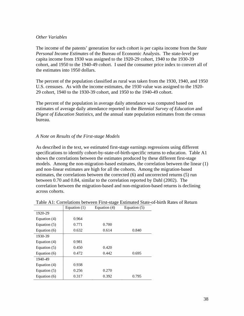
A Note on Results of the First-stage Models

As described in the text, we estimated first-stage earnings regressions using different specifications to identify cohort-by-state-of-birth-specific returns to education. Table A1 shows the correlations between the estimates produced by these different first-stage models. Among the non-migration-based estimates, the correlation between the linear (1) and non-linear estimates are high for all the cohorts. Among the migration-based estimates, the correlations between the corrected (6) and uncorrected returns (5) run between 0.70 and 0.84, similar to the correlation reported by Dahl (2002). The correlation between the migration-based and non-migration-based returns is declining across cohorts. Table A1: Correlations between First-stage Estimated State-of-birth Rates of Return Equation (1) Equation (4) Equation (5) 1920-29 Equation (4) 0.964 Equation (5) 0.771 0.700 Equation (6) 0.632 0.614 0.840 1930-39 Equation (4) 0.981 Equation (5) 0.450 0.420 Equation (6) 0.472 0.442 0.695 1940-49 Equation (4) 0.938 Equation (5) 0.256 0.270 Equation (6) 0.317 0.392 0.795

38

REFERENCES

Alesina, Alberto, Reza Baqir, and Caroline Hoxby. 2004. “Political Jurisdictions in

Heterogeneous Communities.” Journal of Political Economy 112: 348-396.

Andrews, Mathew, William Duncombe, and John Yinger. 2002. “Revisiting Economies

of Size in American Education: Are We Any Closer to a Consensus?” Economics

of Education Review 21, 245-262.

Brasington, David. 1999. “The Joint Provision of Public Goods: The Consolidation of

School Districts.” Journal of Public Economics 73, 373-393.

Card, David, and Alan Krueger. 1992. “Does School Quality Mattter: Returns to

Education and the Characteristics of Public Schools in the United States.” Journal

of Political Economy 100, 1-40.

Card, David, and Alan Krueger. 1996. “Labor Market Effects of School Quality: Theory

and Evidence.” In Gary Burtless, Ed., Does Money Matter? The Effect of School

Resources on Student Achievement and Adult Success. Washington DC:

Brookings Institution Press, 97-140.

Conant, James B. 1959. The American High School Today: A First Report to Interested

Citizens. New York, NY: McGraw Hill Book Company.

Conant, James B. 1967. The Comprehensive High School. New York, NY: McGraw Hill

Book Company.

Cotton, Kathleen. 1996. “School Size, School Climate, and Student Performance.”

School Improvement Research Series, Office of Educational Research and

Improvement.

Cubberley, Ellwood P. 1922. A Brief History of Education. Boston: Houghton-Mifflin.

Dahl, Gordon, B. 2002. “Mobility and the Return to Education: Testing a Roy Model

with Multiple Markets.” Econometrica 70(6), 2367-2420.

Duncombe, William, and John Yinger. 2001. “Does School District Consolidation Cut

Costs?” Syracuse University, Center for Policy Research, Working Paper No. 33.

Ferguson, R. F. 1991. Paying for Public Education: New Evidence on How and Why

Money Matters. Harvard Journal of Legislation, 28, 466–498.

39

Ferguson, R. F., and Ladd, H. F. 1996. Additional Evidence on How and Why Money

Matters: A Production Function Analysis of Alabama Schools. In H. F. Ladd,

Holding Schools Accountable: Performance-Based Reform in Education.

Fox, W. F. 1981. “Reviewing Economies of Size in Education.” Journal of Education

Finance, 6.

Hanusheck, Eric, Steven Rivkin, and Lori Taylor. 1996. “Aggregation and the Estimated

Effects of School Resources.” Review of Economics and Statistics 78, 611-627.

Heckman, James, Anne Layne-Farrar, and Petra Todd. 1996. “Human Capital Pricing

Equations with an Application to Estimating the Effect of School Quality on

Earnings,” Review of Economics and Statistics 78, 562-610.

Hooker, Clifford, and Van Mueller. 1970. The Relationship of School District

Reorganization to State Aid Distribution Systems. National Education Finance

Project Special Study No. 11.

Howley, Craig. 1996. “Review of the Relevant Research.” Doctoal Disstertation, Chapter

2, accessed at http://oak.cats.ohiou.edu/~howleyc/chapter2.htm.

Hoxby, Caroline. 2000. “Does Competition among Public Schools Benefit Students and

Taxpayers?” American Economic Review 90, 1209-1238.

Kenny, Lawrence. 1982. Economies of Scale in Schooling. Economics of Education

Review 2, 1–24.

Kenny, Lawrence, and Amy Schmidt. 1994. “The Decline in the Number of School

Districts in the U.S.: 1950-1980.” Public Choice 79, 1-18.

Lee, V. E., and J. B. Smith 1997. High School Size: Which Works Best and for Whom?

Educational Evaluation and Policy Analysis 19, 205–227.

National Commission on School District Reorganization. 1948. Your School District.

Washington DC: Department of Rural Education, National Education Association

of the United States

Reynolds, David. 1999. There Goes the Neighborhood: Rural School Consolidation at

the Grass Roots in Early Twentieth-Century Iowa. Iowa City: University of Iowa

Press.

Sebold, F. D., and W. Dato. 1981. School Funding and Student Achievement: An

Empirical Analysis. Public Finance Quarterly 9, 91–105.

40

Stock, James H. and Mark W. Watson. 2003. Introduction to Economterics. Boston:

Addison Wesley.

Strang, David. 1987. “The Administrative Transformation of American Education:

School District Consolidation, 1938-1980.” Administrative Science Quarterly 32,

352-366.

Summers, Anita A., and Barbara L. Wolfe. 1977. Do Schools Make a Difference?

American Economic Review 67, 639–652.

Toch, Thomas. 2004. High Schools on a Human Scale: How Small Schools can

Transform American Education. Boston, MA: Beacon Press.

Tyack, David. 1974. The One Best System: A History of American Urban Education.

Cambridge, MA: Harvard University Press.

U.S. Department of Education, Digest of Education Statistics 2002.

Walberg, Herbert. J., and William J. Fowler. 1987. Expenditure and Size Efficiencies of

public School Districts. Educational Researcher 16, 5–13.

41

Figure 1

050

100

150

200

250

Num

ber o

f Sch

ools

(100

0s)

1870 1880 1890 1900 1910 1920 1930 1940 1950 1960 1970 1980 1990 2000Year

All Schools One-Teacher Schools

Data for one-teacher schools only available after 1927.

Number of Public Schools, 1869-1999

Figure 2

020

4060

8010

012

0N

umbe

r of S

choo

l Dis

trict

s (1

000s

)

1930 1940 1950 1960 1970 1980 1990 2000Year

Number of School Districts, 1931-1999

42

Figure 3

01

23

45

Avg

. Dai

ly A

ttend

ance

per

Sch

ool (

100s

)

1870 1880 1890 1900 1910 1920 1930 1940 1950 1960 1970 1980 1990 2000Year

Average School Size, 1869-1999

Figure 4

01

23

Avg

. Dai

ly A

ttend

ance

per

Dis

trict

(100

0s)

1930 1940 1950 1960 1970 1980 1990 2000Year

Average District Size, 1931-1999

43

Figure 5

010

2030

4050

6070

80S

hare

of R

even

ue (P

erce

nt)

1920 1940 1960 1980 2000Year

Local State Federal

Sources of Public Education Funding, 1919-1998

44

Table 1: Spearman Rank Correlations among School Characteristics by Cohort School

size (ADA)

District size

(ADA)

State share of funding

Pupil-teacher

ratio

Term length

1920-29 0.703 District size (ADA)

(0.000) 0.408 0.524 State share of funding

(0.004) (0.000) 0.595 0.627 0.723 Pupil-teacher ratio

(0.000) (0.000) (0.000) 0.215 -0.063 -0.358 -0.401 Term length

(0.142) (0.671) (0.013) (0.005) 0.679 0.342 -0.031 0.020 0.624 Relative teacher salary

(0.000) (0.017) (0.836) (0.890) (0.000) 1930-39

0.673 District size (ADA) (0.000) 0.358 0.614 State share of funding

(0.013) (0.000) 0.497 0.668 0.800 Pupil-teacher ratio

(0.000) (0.000) (0.000) 0.362 0.051 -0.251 -0.273 Term length

(0.012) (0.729) (0.086) (0.061) 0.750 0.323 -0.016 0.030 0.536 Relative teacher salary

(0.000) (0.025) (0.917) (0.840) (0.000) 1940-49

0.631 District size (ADA) (0.000) 0.365 0.685 State share of funding

(0.011) (0.000) 0.362 0.706 0.713 Pupil-teacher ratio

(0.012) (0.000) (0.000) 0.404 0.182 0.035 0.170 Term length

(0.004) (0.216) (0.814) (0.248) 0.766 0.381 0.154 0.027 0.405 Relative teacher salary

(0.000) (0.008) (0.296) (0.854) (0.004) Notes: P-values in parentheses. ADA = average daily attendance. All correlations exclude the District of Columbia, Alaska, and Hawaii.

45

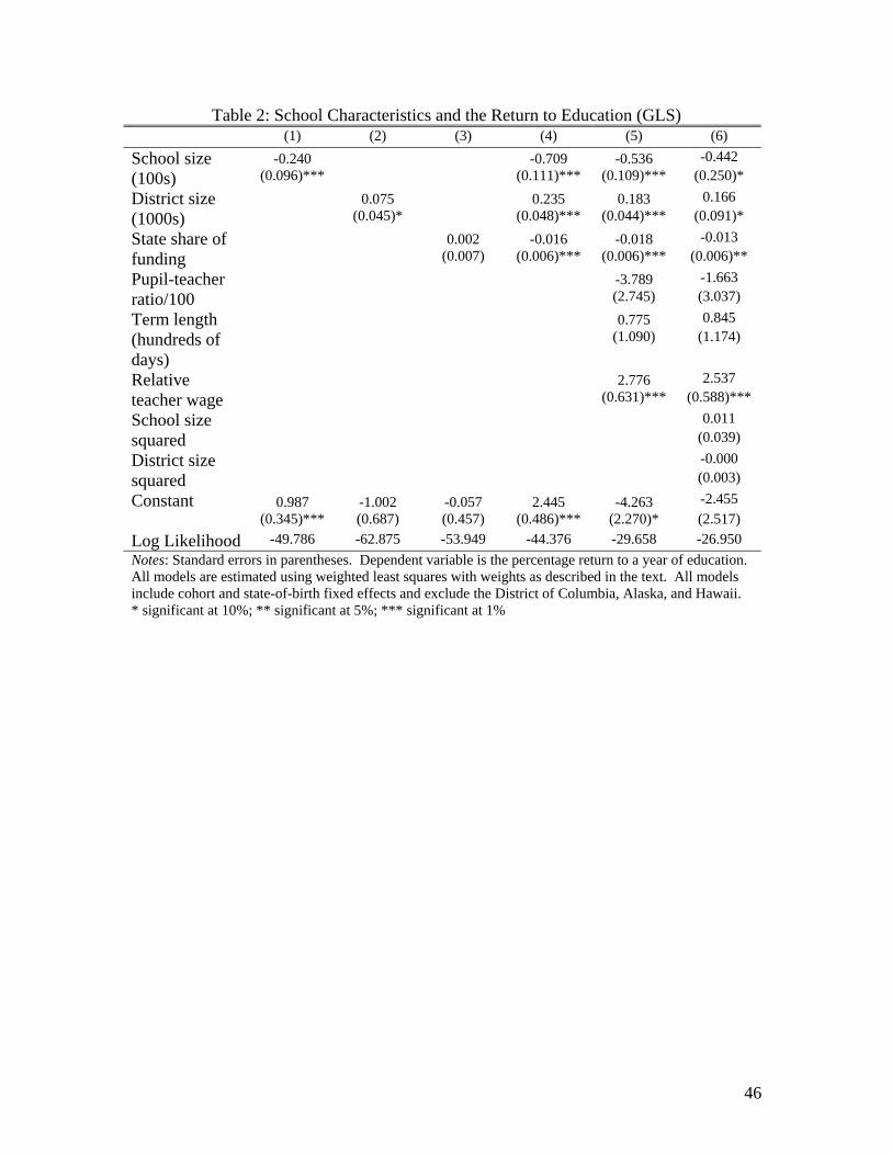
Table 2: School Characteristics and the Return to Education (GLS) (1) (2) (3) (4) (5) (6)

-0.240 -0.709 -0.536 -0.442 School size (100s) (0.096)*** (0.111)*** (0.109)*** (0.250)*

0.075 0.235 0.183 0.166 District size (1000s) (0.045)* (0.048)*** (0.044)*** (0.091)*

0.002 -0.016 -0.018 -0.013 State share of funding (0.007) (0.006)*** (0.006)*** (0.006)**

-3.789 -1.663 Pupil-teacher ratio/100 (2.745) (3.037)

0.775 0.845 Term length (hundreds of days)

(1.090) (1.174)

2.776 2.537 Relative teacher wage (0.631)*** (0.588)***

0.011 School size squared (0.039)

-0.000 District size squared (0.003)

Constant 0.987 -1.002 -0.057 2.445 -4.263 -2.455 (0.345)*** (0.687) (0.457) (0.486)*** (2.270)* (2.517) Log Likelihood -49.786 -62.875 -53.949 -44.376 -29.658 -26.950 Notes: Standard errors in parentheses. Dependent variable is the percentage return to a year of education. All models are estimated using weighted least squares with weights as described in the text. All models include cohort and state-of-birth fixed effects and exclude the District of Columbia, Alaska, and Hawaii. * significant at 10%; ** significant at 5%; *** significant at 1%

46

Table 3: Spearman Rank Correlations between School Characteristics and Population Characteristics 1920-29 1930-39 1940-49

Real percapita

income of

parents

Percent rural

Percent in

school

Real per capita

income of

parents

Percent rural

Percent in

school

Real per capita

income of

parents

Percent rural

Percent in school

Percent rural -0.854 -0.840 -0.712 (0.000) (0.000) (0.000)Percent in school -0.818 0.809 -0.792 0.823 -0.520 0.639 (0.000) (0.000) (0.000) (0.000) (0.000) (0.000)School size (ADA) 0.341 -0.562 -0.284 0.468 -0.589 -0.315 0.366 -0.700 -0.223 (0.179) (0.000) (0.051) (0.008) (0.000) (0.029) (0.011) (0.000) (0.127)District size (ADA) 0.011 -0.214 -0.106 -0.001 -0.118 0.046 -0.223 -0.159 0.183 (0.941) (0.144) (0.472) (0.992) (0.423) (0.759) (0.127) (0.280) (0.214)State share of funding -0.367 0.186 0.238 -0.357 0.277 0.370 -0.350 0.114 0.423 (0.010) (0.205) (0.104) (0.013) (0.056) (0.010) (0.015) (0.442) (0.003)Pupil-teacher ratio -0.377 0.085 0.208 -0.365 0.196 0.381 -0.557 0.147 0.470 (0.008) (0.568) (0.156) (0.011) (0.182) (0.008) (0.000) (0.319) (0.001)Term length 0.860 -0.729 -0.722 0.751 -0.688 -0.670 0.422 -0.475 -0.432 (0.000) (0.000) (0.000) (0.000) (0.000) (0.000) (0.003) (0.000) (0.002)Relative teacher salary 0.761 -0.785 -0.635 0.701 -0.707 -0.527 0.469 -0.678 -0.298 (0.000) (0.000) (0.000) (0.000) (0.000) (0.000) (0.000) (0.000) (0.040)Notes: P-values in parentheses. ADA = average daily attendance. All correlations exclude the District of Columbia, Alaska, and Hawaii.

47

Table 4: Population Characteristics and the Return to Education (GLS)

(1) (2) (3) (4) -0.540 -0.364 -0.502 -0.352 School size (100s)

(0.109)*** (0.106)*** (0.124)*** (0.116)*** 0.185 0.194 0.182 0.202 District size (1000s)

(0.044)*** (0.041)*** (0.044)*** (0.040)*** -0.017 -0.015 -0.017 -0.013 State share of funding

(0.006)*** (0.005)*** (0.006)*** (0.005)** -4.482 -1.071 -3.072 -2.324 Pupil-teacher ratio/100 (2.820) (2.590) (3.024) (2.803) 0.753 1.240 0.872 1.251 Term length (hundreds of

days) (1.087) (1.010) (1.103) (0.999) 2.725 3.846 2.753 3.866 Relative teacher wage

(0.631)*** (0.620)*** (0.632)*** (0.611)*** 0.327 0.762 Real per capita income of

parents’ generation ($1000s)

(0.323) (0.303)**

4.374 4.944 Rural population (percent) (0.874)*** (0.891)*** -3.502 -0.077 Percent of population

attending School (ADA)

(6.244) (5.693)

-1.394 -9.669 -4.200 -10.486 Constant (2.140) (2.356)*** (2.270)* (2.341)***

Observations 144 144 144 144 Log Likelihood -29.149 -18.110 -29.501 -15.020 Notes: Standard errors in parentheses. Dependent variable is the percentage return to a year of education. All models include cohort and state-of-birth fixed effects and the District of Columbia, Alaska, and Hawaii. All models are estimated using weighted least squares with weights as described in the text. * significant at 10%; ** significant at 5%; *** significant at 1%

48

Table 5: School Characteristics and the Linear Base Rate of Return to Education (GLS), Models Allowing for Sheepskin Effects for High School and College Degrees

(1) (2) (3) (4)

-0.383 -0.177 -0.616 -0.406 School size (100s)

(0.222)* (0.245) (0.115)*** (0.119)*** 0.077 -0.058 0.188 0.212 District size (1000s)

(0.090) (0.085) (.047)*** (0.041)*** -0.030 -0.027 -.0139 -0.009 State share of funding

(0.011)*** (0.012)*** (0.006)*** (0.006) 1.743 5.227 -1.248 -0.078 Pupil-teacher ratio/100

(5.600) (5.955) (2.905) (2.869) -1.966 -1.391 0.065 0.597 Term length (hundreds of

days) (2.245) (2.127) (1.155) (1.023) 2.869 4.802 2.063 3.304 Relative teacher wage

(1.298)** (1.297)*** (0.669)*** (0.625)*** -0.391 1.123 Real per capita income of

parents generation ($1000s) (0.638) (0.310)***

7.496 5.774 Rural population (percent)

(1.887)*** (0.912)*** 10.357 0.118 Percent of population in

school (ADA) (12.106) (5.827) 1.577 -6.567 -0.140 -10.243 Constant

(4.596) (4.790) (2.370) (2.400)*** First-stage model includes cohort X sheepskin effects for high school and college degrees?

Y Y Y Y

First-stage model includes region X sheepskin interactions?

Y Y Y Y

First-stage model includes cohort X state-of-birth X sheepskin effect interactions?

Y Y N N

Observations 144 144 144 144 Log Likelihood -131.862 -122.908 -37.802 -18.275 All models are estimated using weighted least squares with weights as described in the text. All models include cohort and state-of-birth fixed effects and exclude the District of Columbia, Alaska, and Hawaii. * significant at 10%; ** significant at 5%; *** significant at 1%

49

Table 6: School System Characteristics and the Return to Education (GLS), Migration-based Estimates (1) (2) (3) (4)

Migrant-based returns Returns Corrected for Selective Migration

-0.507 -0.418 -0.636 -0.517 School size (100s) (0.116)*** (0.119)*** (0.132)*** (0.138)***

0.123 0.119 0.063 0.059 District size (1000s) (0.047)*** 0.044*** (0.054) (0.051)

-0.009 -0.013 -0.007 -0.011 State share of funding (0.008) (0.007)* (0.009) (0.009) -10.306 -7.800 -6.064 -3.175 Pupil-teacher ratio/100

(3.285)*** (3.177)** (3.821) (3.746) 0.374 0.443 -2.218 -2.076 Term length (hundreds of days)

(1.102) (1.031) (1.254)* (1.202)* 0.135 1.638 0.645 2.231 Relative teacher wage

(0.622) (0.652) (0.705) (0.765)* -1.249 -1.260 Real per capita income of

parents’ generation ($1000s) (0.411)*** (0.493)***

3.881 3.973 Rural population (percent) (1.142)*** (1.351)*** 3.988 -0.878 Percent of population attending

School (ADA) (6.406) (7.523) 7.347 6.086 10.988 7.958 Constant

(2.469)*** (2.482)** (2.837)*** (2.909)*** Observations 144 144 144 144 Log Likelihood -51.235 -38.675 -70.553 -61.426 All models are estimated using weighted least squares with weights as described in the text. All models include cohort and state-of-birth fixed effects and exclude the District of Columbia, Alaska, and Hawaii. * significant at 10%; ** significant at 5%; *** significant at 1%

50

Table 7: Determinants of Educational Attainment (GLS) (1) (2) (3) (4) Dropouts Years of Education

0.022 0.022 -0.078 -0.084 School size (100s) (0.007)*** (0.007)*** (.040)** (0.039)**

-0.006 -0.006 0.016 0.009 District size (1000s) 0.003** (0.003)** 0.016 0.016 -0.000 -0.000 -(0.001) 0.000 State share of funding (0.000) (0.000) 0.003 (0.003) 1.141 1.100 -7.215 -6.970 Pupil-teacher ratio/100

(0.185)*** (0.187)*** (1.138)*** (1.127)*** -0.035 -0.027 -0.031 -0.190 Term length (hundreds

of days) (0.061) (0.061) (0.376) (0.371) -0.076 -0.082 0.742 0.681 Relative teacher wage

(0.036)** (0.041)** 0.210*** (0.236)*** 0.035 -0.374 Real per capita

income of parents’ generation ($1000s) (0.025) (0.151)**

0.019 -0.759 Rural population (percent) (0.069) (0.418)*

0.237 0.194 13.057 14.243 Constant (0.138) (0.159) (0.849)*** (0.896)***

Observations 144 144 144 144 Log Likelihood 364.404 365.471 103.211 107.091 Notes: Standard errors in parentheses. Dependent variable is the percentage of the population receiving 11 years of education or less (columns 1-3) or average years of education (columns 3-4). All models include cohort and state-of-birth fixed effects and exclude the District of Columbia, Alaska, and Hawaii. Observations are weighted based on the number of white males from each state in the relevant birth cohort using the method described in the text. * significant at 10%; ** significant at 5%; *** significant at 1%

51

Table 8: Reduced-Form Estimates of the Effects of School Characteristics on Earnings

(1) (2) (3) (4) (5)

-(0.013) -0.013 -0.011 School size (100s) (0.002)*** (0.002)*** (0.002)***

-0.001 0.0002 -0.001 District size (1000s) (0.0007) (0.0007) (0.001) 0.0002 0.0001 -0.0002 State share of funding (0.0002) (0.0002) (0.0002) -0.479 Pupil-teacher ratio/100 (0.070)*** 0.012 Term length (hundreds of

days) (0.023) 0.031 Relative teacher wage (0.010)***

3.971 3.919 3.909 3.966 4.023 Constant (0.022)*** (0.021)*** (0.021)*** (0.023)*** (0.051)***

Observations 994883 994883 994883 994883 994883 Adjusted R2 0.0929 0.0928 0.0928 0.0929 0.0929 Notes: Standard errors in parentheses. All models include age and its square, a current marital status indicator, and an indicator of residence in an SMSA along with cohort, state-of-residence, and state-of-birth fixed effects. * significant at 10%; ** significant at 5%; *** significant at 1%

52

Table A1: Summary Statistics

Cohort District Size

(ADA) School Size

(ADA) State Share of Funding

Pupil-Teacher

Ratio Term Length

(Days)

Relative Teacher Wage

Real Income of Parents' Generation

Percent Rural

Percent of Population

in ADA

Percent without a

high school degree

Average Years of

Education 1920-29

Mean 1,290

108 26.7 28.2 172 0.92 $540 54.0 17.6 36.3 11.8Median 236 92 24.8 28.2 175 0.89 $60 60.0 17.6 34.1 12.0

SD 2,075

64 18.3 4.9 10 0.20 $199 19.9 2.2 10.8 0.8Min 34 26 1.1 17.7 139 0.65 $291 7.6 13.8 20.7 10.0Max 10,587

293 90.8 37.6 187 1.54 $1,490 83.4 23.0 58.2 13.3

1930-39 Mean 1,598

148 37.1 26.2 175 0.96 $930 52.7 16.7 23.7 12.6

Median 468 141 36.6 26.8 176

0.96 $895 57.7 16.7 21.5 12.8SD 2,492

81 21.2 3.9 6 0.15 $330 18.3 2.4 8.0 7.0

Min 33 29 2.3 16.6 154 0.66 $370 8.4 12.1 12.5 10.9Max 12,520

332 89.8 34.4 187 1.30 $1770 80.2 22.0 44.8 13.9

1940-49 Mean 2,394 244 38.1 25.0 178 0.97 $1,421 44.4 18.2 14.2 13.5

Median 1,183 237 34.8 25.5 178

0.96 $1,432 45.4 18.4 12.5 13.6SD 1,146

115 18.4 3.0 3 0.11 $316 16.0 2.3 6.0 0.6

Min 40 42 3.5 17.6 168 0.76 $770 13.4 13.0 6.6 12.1Max 19,654 508 84.9 31.4 184 1.19 $2,075 73.4 23.5 30.9 14.4

Notes: Income of parents’ generation is expressed in 1950 dollars. ADA = average daily attendance. Washington, D.C. is excluded throughout.

53