Embed Size (px)
Citation preview
ERGEBNISSE DER MATHEMATIK UND IHRER GRENZGEBIETE
PUBLISHED UNDER THE EDITORSHIP OF THE
“ZENTRALBLATT FÜR MATHEMATIK” VOLUME FOUR
_____________________________ 2 _____________________________
GROUPS OF LINEAR TRANSFORMATIONS
BY
B. L. VAN DER WAERDEN
Translated by D. H. Delphenich
CHELSEA PUBLISHING COMPANY 231 WEST 29TH STREET, NEW YORK 1, N. Y.
1948
Table of contents
Page I. Linear groups in arbitrary fields………………………………………….... 1 § 1. Linear transformations…………………………………………………. 1 § 2. The general and special linear group………………………………….. 5 § 3. The projective group…………………………………………………… 7 § 4. The complex group…………………………………………………….. 10 § 5. The unitary group……………………………………………………..... 11 § 6. The orthogonal groups…………………………………………………. 14 § 7. The isomorphisms of the orthogonal groups in dimensions 3, 4, 5, and 6 § 8. Linear groups in complex number fields. Reducible and irreducible, primitive, imprimitive, and monomial groups………………………….. 19 § 9. Finite, linear groups of given degrees…………………………………… 31 § 10. Infinite, discrete groups of fractional linear transformations, in particular, discrete groups of motions……………………………………………….. 34 II. Representations of rings and groups………………………………………… 44 § 11. Representations and representation modules…………………………….. 44 § 12. Representations of hypercomplex systems. Semi-groups of linear
transformations…………………………………………………………… 50 § 13. Representations of finite groups………………………………………….. 55 § 14. Restricted representations of arbitrary groups……………………………. 59 § 15. Traces and characters…………………………………………………….. 66 § 16. The decomposition of irreducible representations by extension of the ground field……………………………………………………………….. 71 § 17. Factor systems……………………………………………………………. 74 § 18. Integrality properties. Modular representations…………………………. 77 § 19. Relations between the representations of a group and those of its subgroups. Imprimitive representations………………………………….. 79 § 20. Representations of special groups………………………………………… 83 § 21. Representations of groups by projective transformations………………… 87 § 22. The rational representations of the general linear group…………………. 92
I. Linear groups in arbitrary fields.
The source for the theory of linear groups in finite fields (i.e., Galois fields) is, to this day, the book of DICKSON (1). Later on, DICKSON himself adapted many of his results to infinite fields. However, a complete overview of this domain that likewise clearly emphasizes the relationships with the theory of continuous groups and projective geometry does not exist. On those grounds, the subject of the exposition that follows will be that of treating the recent work once more from its foundations, in which, however, some of the details – in particular, the proofs of the simplicity of the groups examined – will be referred to the DICKSON book. The isomorphisms of the orthogonal groups in the singular cases n = 3, 4, 5, 6, which make up an attractive part of the DICKSON book, will be derived below from the ground up, while emphasizing their abundant geometric and algebraic relationships. The last paragraphs will treat the encyclopedia article of A. WIMAN and R. FRICKE on the discrete groups of linear transformations with complex number coefficients, while expanding it with discussions of recent investigations.
§ 1. Linear transformations (2).
One understands an n-dimensional vector space En(K) over a field K to mean an
additive Abelian group (whose elements are called vectors) with K as an operator domain
that (in addition to the axioms of an Abelian group) satisfies the following axioms (u, v,
… are vectors, while 1, α, β, … are elements of K):
1. (u + v) α = uα + vα, 2. u (α + β) = uα + uβ, 3. u (αβ) = (uα) β, 4. u 1 = u. 5. There are n “basis vectors” u1, …, un such that any vector v can be written as a unique linear combination:
v = 1
n
uν νν
ξ=∑ .
Two vector spaces are operator-isomorphic over K if and only if they have the same
dimension n (i.e., the same linear rank). One can then take an arbitrary n-dimensional
(1) L. E. DICKSON, Linear Groups, with an exposition of the Galois field theory, Leipzig, 1901. (2) The basic concepts of linear algebra that will be needed in what follows will all be briefly summarized in this paragraph. For a thorough presentation, see, perhaps, B. L. VAN DER WAERDEN: Moderne Algebra II, Berlin, 1931, chap. 15, or L. E. DICKSON, Modern algebraic theories, Chicago, 1926.
2 I. Linear groups in arbitrary fields.
vector space to be a model for all of them by defining a vector to be – say – a linear form
1
n
uν νν
ξ=∑ in n indeterminates u1, …, un .
The admissible subgroups of a vector space R (relative to K as an operator domain)
are called linear subspaces or subspaces of R. Moreover, the proper subspaces are
vector spaces of dimension m < n. It follows from this that any decreasing or increasing sequence of subspaces will truncate after a finite number of them. The homomorphic maps of a vector space R to a vector space S will be called linear
transformations of R to S. A linear transformation is then a map A of R to S for which
one has: A (u + v) = Au + Av, A (u α) = (A u) α. For an arbitrary choice of bases (u1, …, un) and (v1, …, vm) for R and S, resp., a
linear transformation A that takes uk to:
A uk = j jkj
v α∑
will be given completely by its matrix A = (αjk) (j is the row index, and k is the column index): Namely, it will then necessarily take the vector k ku ξ∑ with components ξk to
the vector ( )k ku ξ∑ A = k kv ξ ′∑ with the components:
(1) jξ ′ = jk k
j
α ξ∑ .
The product AB of two linear transformations will then correspond to the product AB of the matrices (naturally, assuming that the product is meaningful; i.e., that A indeed operates on the image space of B). On the basis for formula (1), one can also regard any linear transformation as a linear substitution of the variables ξ1, …, ξn that takes ξ1, …, ξn to 1ξ ′ , …, mξ ′ . This way of
looking at things will then be employed, in particular, when m = n, so A will become a square matrix of degree n (i.e., with n rows and columns). If the transformation A takes the n basis vectors u1, …, un to linearly-dependent basis vectors, so the vector space R goes to a space of lower dimension, then the
transformation will be called singular. A non-singular transformation A will map R to
an image space of the same dimension in a one-to-one manner, and will possess an inverse A−1 such that A−1 A = A A−1 = I (i.e., the identity).
The linear transformations of a vector space En(K) into itself (or their matrices)
define a ring: viz., the full matrix ring of degree n over K. This ring can be regarded as a
§ 1. Linear transformations. 3
hypercomplex system with n2 basis elements, for which one can choose, e.g., the n2 matrix units Cik that have a one in the i th row and kth column, but zero everywhere else. These matrices Cik satisfy the rules of calculation: Cik Ckl = Cil , Cij Ckl = 0 for j ≠ k. The unity element of the ring is I = C11 + C22 + … + Cnn . From now on, we will consider only linear transformations of a vector space R =
En(K) into itself and also assume that the field K is commutative.
One understands the characteristic polynomial χ(t) of a square matrix A to mean the determinant of tI – A. The individual coefficients of this characteristic polynomial − in particular, the trace S(A) = ννα∑ and the norm, or determinant, | A | − are invariant
under the transformations TAT−1. The zeroes of χ(t), in a suitable extension field of K,
are called the characteristic roots of the matrix A. One achieves the classification of linear transformations with the help of their elementary parts most easily when one regards the vector space R in which a given linear
transformation A lives as an additive Abelian group with the polynomial domain K[A] as
its operator domain and then applies the main theorem of the decomposition of Abelian groups into cyclic ones. Here, I will briefly give only the main result, and refer to the textbooks (2) for the proof. The minimal polynomial of A – i.e., the polynomial of smallest degree ϕ(t) for which one has ϕ(A) = 0 – is a divisor of the characteristic polynomial of the matrix A. If one decomposes ϕ(t) into factors that are powers of prime polynomials:
ϕ(t) = ϕ1(t) … ϕs(t), ϕk(t) = ( ) krk tπ
then the space R will decompose uniquely into subspaces:
R = R1 + R2 + … + Rs
(i.e., a direct sum, in the sense of group theory), in which Rk will be annihilated by ϕk(A):
ϕk(A) Rk = 0. Any space Rk will decompose further into “cyclic” subspaces rν , each of
which will be spanned by a vector vν and its transforms Avν . Each will be associated with an annihilating polynomial of lowest degree ψv(t) = ( )e
k t νπ . The minimal
polynomials ψv will be the elementary divisors of the matrix tI – A. Their product will be the characteristic polynomial χ(t). Any matrix A can be brought into a normal form that depends upon only elementary divisors by a transformation TAT−1; in this expression, T, as well as A, will be a matrix
with coefficients in K. On the basis of that normal form (or on the basis of the reasoning
4 I. Linear groups in arbitrary fields.
that leads up to it), one can exhibit the linear transformations that commute with a given linear transformation A (3). An important special case of the theory of elementary divisors then emerges when all elementary divisors become linear by the adjunction of the characteristic roots to the field
K. In that case, the normal form of A will be a diagonal matrix in whose diagonal one
will find the characteristic roots. This case shows up, in particular, when Ah = I and h is
relatively prime to the characteristic of K. If several matrices with linear elementary
divisors commute with each other then one can bring them into diagonal form simultaneously. Special case: For the fields of complex or algebraic numbers, any periodic linear transformation, and similarly, any finite Abelian group of linear transformations, can be transformed into diagonal form (with roots of unity in the diagonal). A generalization of linear transformations that has been examined only slightly up to now, but which nevertheless plays a role in very many places in mathematics, is defined by the semi-linear transformations, which one obtains when one combines linear
transformations with automorphisms of the ground field K. If So is such an
automorphism then the formula: (2) iξ ′ = S
ik kα ξ∑
will define a semi-linear transformation. In particular, if K is the field of complex
numbers and S is the transition to complex conjugates then one will speak of an anti-linear transformation. If A and B are semi-linear transformations that belong to the automorphisms S and T, resp., and are given by the matrices A and B, resp., moreover, then the product AB will belong to the automorphism ST and the matrix ABS, where BS arises from B by subjecting all elements of the matrix B to the automorphism S. In particular, the product of two anti-linear transformations will be a linear transformation with the matrix AB. A classification of the semi-linear transformations − or even just the anti-linear ones, in particular − by the theory of elementary divisors still does not seem to exist. It is only for those anti-linear transformations whose square is a transformation λI that one knows normal forms into which they can all be transformed (4). The dual space to a vector space En consists of all linear functions of a vector (or its
components) whose values belong to the same field K. If v = uν νξ∑ is an arbitrary
vector then:
l = 1
nν
νν
λ ξ=∑
(3) A long series of papers by various authors treated this theme, starting with G. FROBENIUS: J. reine angew. Math. 84 (1878), 1-63. For the literature, see C. C. MacDUFFEE: Theory of Matrices, Ergebn. d. Math. 2, H. 5 (1933), 93. For extensions of that, let us mention the papers of O. SCHREIER and B. L. VAN DER WAERDEN: Abh. Math. Inst. Hamburg 6 (1928), 308-310 and K. SHODA: Math. Z. 29 (1929), 696-712. (4) E. JACOBSTHAL: S.-B. Berl. math. Ges. 33 (1934), 15-34.
§ 2. The general and special linear group. 5
will be an arbitrary linear function of v. A vector in the dual space will then given by n components λ1, …, λn. A non-singular linear transformation of the given vector space into itself will necessarily induce a linear transformation of the dual space whose matrix is the transposed inverse of the matrix of the given transformation. A non-singular linear transformation of the vector space En into its dual space is called a duality. It will be given by the formula: (3) ′λi = ik
kδ ξ∑ .
Such a transformation of the space En into its dual space is necessarily coupled with a transformation of the dual space into the original En whose matrix is again the transposed inverse of the matrix (δik) of the given duality. We will refer to these two associated transformations together as one duality. One can now multiply dualities and linear transformations, which must likewise be taken together with the linear transformations that they induce on the dual space, with each other arbitrarily. The composition of two dualities – e.g. – will yield a linear transformation of En into itself.
If one composes the dualities with the automorphisms S of the ground field K then
one will obtain dualities in the extended sense: (4) ′λi = ik S
kδ ξ∑ .
The non-singular, semi-linear transformations and the dualities in the extended sense collectively define a group.
§ 2. The general and special linear group.
The non-singular, linear transformations of the vector space En(K) into itself define a
group: viz., the general linear group GL(n, K) (5). As always in what follows, if we
assume that the field K is commutative then the transformations with determinant one
will define a subgroup: viz., the special linear group SL(n, K). For n > 1, SL(n, K) will
be the commutator group of GL(n, K), although in the one case of n = 2, one assumes that
K = GF(2) (6). The group SL(n, K) will be generated by the transformations:
(5) The notation is borrowed from the American school (cf., L. E. DICKSON: Linear Groups, Leipzig, 1901); nonetheless, some notations will be simplified and others converted systematically. Thus, we shall write GL, instead of GLH (= general linear homogeneous) and SL, instead of SLH. (6) Here and in what follows, GF(q) will always denote the Galois field with q elements. Cf., B. L. VAN DER WAERDEN, Moderne Algebra I, § 31.
6 I. Linear groups in arbitrary fields.
Br, s, λ : for .
r s
rν
ν ν
ξ ξ λξξ ξ ν
′ = + ′ = ≠
In order to generate GL(n, K), one must add the transformations:
1 1 ( 0),
for 1.ν ν
ξ λξ λξ ξ ν
′ = ≠ ′ = ≠
L. E. DICKSON (7) has presented the defining relations of the groups SL(n, K).
The center of GL(m, K) consists of the transformations λI, where I is the identity.
The center of SL(n, K) consists of the transformations λI, where λ is an nth root of unity.
We will thoroughly discuss the factor group of SL(n, K) by its center in § 3.
The classification of linear transformations by their elementary divisors that was discussed in § 1 simultaneously provides the partitioning of the elements of the group
GL(n, K) into conjugacy classes.
If K is a finite field GF(q), q = pm then GL(n, K) and SL(n, K) will be finite groups of
order: (qn – 1) (qn − q) … (qn – qn−1) (q = pm), or (qn – 1) (qn − q) … (qn – qn−2) qn−1, resp. These groups will also be denoted by GL(n, pm) [SL(n, pm), resp.]. The group SL(2, p) is the “group of binary congruences” with prime number modulus p. L. E. DICKSON (8) has determined the subgroups of SL(n, pm). C. JORDAN (9) and G. BUCHT (10) treated the maximal solvable subgroups of the group GL(n, p). We will learn about some other important subgroups in §§ 4-6. For the case of the field of complex numbers, see also §§ 7 and 8.
One obtains extensions of the group GL(n, K) by adding the semi-linear
transformations (dualities, resp.) (cf., § 1).
(7) L. E. DICKSON: Bull. Amer. math. Soc. (2) 13 (1907), 386-389 – Quart; J. Math. 38 (1907), 141-145. (8) L. E. DICKSON: Amer. J. Math. 33 (1911), 175-192. (9) C. JORDAN: J. de Math. (7) 8 (1917), 263-374. (10) G. BUCHT: Ark. Mat. Astron. Fys. 11 (1917), no. 26.
§ 3. The projective group. 7
§ 3. The projective group.
As is known, the totality of all rays or one-dimensional subspaces that go through the
origin of the vector space En(K) is called the projective space Pn−1(K). The non-singular
linear transformations of En into itself induce projective transformations of Pn−1(K).
Thus, the linear transformations A and λA, where λ is a number, will always yield the same projective transformation.
The totality of all projective transformations of Pn−1(K) is called the n-ary projective
group PGL(n, K) (11). It is isomorphic to the factor group of GL(n, K) by the subgroup
of λI (i.e., the center). Likewise, the factor group of SL(n, K) by its center is called the
special projective group PSL(n, K) (12).
In the case of a finite field GF(q) with q = pm elements, PSL(n, K) = PSL(n, q) is a
finite group of order: 1( 1)( 1) ( )
( 1)
n n n nq q q q
d q
−− − −−⋯
,
where d means the number of nth roots of unity in K: viz., d = (n, q – 1). Since the
projective space contains 1
1
nq
q
−−
points in this case, PGL(n, q) and PSL(n, q) are
permutation groups of degree 1
1
nq
q
−−
. In the case n = 2, one deals with permutation
groups of degree q + 1 and order 2( 1)q q
d
−, in particular. For q = 2, PSL(2, q) is the
symmetric group S3, for q = 3, 4, it is the alternating group A4 (A5, resp.). PSL(2, q) is
not a simple group in either case q = 2, 3. However, one now has the theorem:
If K is a field of characteristic ≠ 2 or a complete field (12a) and n > 1 then the group
PSL(n, K) will be a simple group, except for the lowest cases PSL(2, 2) and PSL(2, 3)
that were just mentioned.
(11) PGL = projective general linear. (12) PSL = projective special linear. The American school writes LF = linear fractional. We have preferred to make the transition from a linear group to the factor group by the substitutions λI that it contains systematically recognizable everywhere by prefixing a P. (12a) For this concept, see E. STEINITZ: J. reine angew. Math. 137 (1910), 181 and 218 or VAN DER WAERDEN (6), § 25 and § 33.
8 I. Linear groups in arbitrary fields.
For the proof, see L. E. DICKSON: Linear Groups (Leipzig, 1901), § 104-105 (13).
For K = GF(pr), one will arrive at an important infinite system of finite, simple
groups on the grounds of this theorem. The smallest of them are the well-known simple groups PSL(2, 4) ≅ PSL(2, 5) and PSL(2, 7) ≅ PSL(3, 2) of orders 60 and 168, resp. E. H. MOORE and A. WIMAN have enumerated the subgroups of the group PSL(2,
q) (14). H. H. MITCHELL (15) determined the finite subgroups of PSL(2, K) for an
arbitrary ground field K by a surprisingly simple method. He thus naturally once more
obtained the results of MOORE and WIMAN as special cases, as well as a known
theorem of KLEIN (cf., § 8) for K = field of complex numbers. In the same paper,
MITCHELL determined the finite subgroups of the group PSL(3, K) for all fields of
characteristic ≠ 2. R. W. HARTLEY (16) determined subgroups of PSL(3, 2n). For the
subgroups of PSL(4, K), see H. H. MITCHELL (17), as well as the literature that is given
in that paper. For the case of the field of complex numbers, see also § 8. One can infer the validity of the assertion that the group PSL(2, q) contains no subgroup of index smaller than q + 1 from the list of subgroups of PSL(2, q), which was first stated without proof by GALOIS, so it can also not be represented as a permutation group of less than q + 1 objects, except in the cases q = 2, 3, 5, 7, 9, 11, for which there will be subgroups of index 2, 3, 5, 7, 6, 11, resp. The associated representations as permutation groups of only q elements are 1-isomorphic, except in the cases q = 2, 3. For q = 5 and q = 9, one will be dealing with the representations of the group PSL(2, q) as an alternating group of 5 (6, resp.) objects: (1) PSL(2, 5) ≅ PSL(2, 4) = A5 ,
(2) PSL(2, 9) ≅ A6 ,
and for q = 7, the representation of the known simple group of order 168 as the permutation group of 7 points in a projective plane: (3) PSL(2, 7) ≅ PSL(3, 2) .
(13) In order to make the proof valid for the case of infinite fields, as well, one must replace 2 2
1 2τ τ+ with
2 2
1 2τ τ− on pp. 97 of the DICKSON book that was cited above. [Cf., L. E. DICKSON: Trans. Amer. Math. Soc. 2 (1901), 368.] (14) E. H. MOORE: Chicago decennial publ. 9 (1904), 141-190. – A. WIMAN: Handl. Svenska Vet.-Akad. 25 (1899), 1-47. The special case q = p (prime number), which is important for the theory of module substitutions, was already resolved before by GIERSTER: Math. Ann. 18 (1881), 319-325. (15) H. H. MITCHELL, Trans. Amer. Math. Soc. 12 (1911), 208-211. (16) R. W. HARTLEY: Ann. of Math. 27 (1925), 140-158. (17) H. H. MITCHELL: Trans. Amer. Math. Soc. 14 (1913), 123-142.
§ 3. The projective group. 9
L. E. DICKSON (18) and W. H. BUSSEY (19) have presented systems of defining relations for the groups PSL(n, q). In the special case of the modular group PSL(2, p), where p is an odd prime number, the BUSSEY relations read simply (20):
S p = T 2 = (ST)3 = 1, (Sτ T Sσ T)2 = 1 for στ ≡ 2 (mod p).
The projective transformations are not, as one often intends, the only transformations of the projective space into itself that transform points to points, lines to lines, planes to planes, etc. They are probably the only ones that will leave the double ratio of four points invariant, in addition. However, along with them, there are transformations that
subject the double ratio to an automorphism of the field K (20a). One gets them when one
applies a semi-linear transformation (§ 1, formula 2) to the coordinates ξ. We would like to call the transformations of projective space thus obtained collineations. The correlations stand beside them, which take points to hyperplanes, and which are induced by dualities, in the extended sense (§ 1, formula 4). Naturally, in fields like the real numbers, in which no automorphism exists besides the identity, any collineation is a projective transformation. The collineations and correlations collectively define a group. According to SCHREIER and V. D. WAERDEN (21), that group will likewise be the group of
automorphisms of the special projective group PSL(n, K). That is: Any automorphism of
the group PSL(n, K) will have the form:
X → CXC−1, where C is a collineation or a correlation. The same investigation yielded that the various
PSL(n, K) exhibited no other isomorphisms between themselves than the ones that were
written down in (1) and (3), and furthermore that only the following ones of the groups PSL were isomorphic to alternating groups An :
PSL(2, 3) ≅ A4, PSL(2, 9) ≅ A6,
PSL(2, 5) ≅ PSL(2, 4) ≅ A5, PSL(4, 2) ≅ A8 .
In particular, the two simple groups PSL(2, 4) and PSL(3, 4) of order 12 8!⋅ are not
isomorphic to each other (22).
(18) L. E. DICKSON: Linear Groups, Leipzig, 1901. § 278 – Proc. London math. Soc. 35 (1903), 292-305, 306-319, and 443-454. (19) W. H. BUSSEY: Proc. London Math. Soc. (2) 3 (1915), 296-315. (20) On this, cf. also H. FRASCH: Math. Ann. 108 (1933), 249-252. Other relations were given by J. A. TODD: J. London Math. Soc. 7 (1932), 195-200. (20a) Cf., F. LEVI: Geometrische Konfigurationen, 1929, § 7. (21) Abh. Math. Sem. Hamburg 6 (1928), 303-322. (22) Cf., also J. M. SCHOTTENFELS: Bull. Amer. Math. Soc. (2) 8 (1902), 25-26.
10 I. Linear groups in arbitrary fields.
§ 4. The complex group.
The group of all linear substitutions of the variables x1, …, xn with coefficients in K
that are performed on two cogredient (i.e., they transform the same) sequences of variables ξ, η and leave an alternating form:
(1) ϕ = 2 1 2 2 2 11
( )m
i i i ii
ξ η ξ η− −=
−∑
invariant is called the complex group C(2m, K) (23). It is also called the ABELian linear
group, after ABEL, who was the first to examine it, but we would like to avoid that terminology, since the group is in no way Abelian. The restriction to the special form (1) is not an essential restriction, since any alternating bilinear form ϕ = ik i kε ξ η∑ with a
determinant | εik | ≠ 0 can be put into the form (1). Obviously, for m = 1, one will have:
C(2, K) = SL(2, K).
For m ≠ 1, C(2m, K) will be generated by the transformations:
Mi : 2 1iξ +′ = ξ2i , 2iξ ′ = − ξ2i−1 , and the remaining kξ ′ = ξk ,
Λi,λ : 2 1iξ −′ = ξ2i−1 + λξ2i , and the remaining kξ ′ = ξk ,
Nij,λ : 2 1 2 1 2
2 1 2 1 2
,
,i i j
j j i
ξ ξ λξξ ξ λξ
− −
− +
′ = + ′ = +
and the remaining kξ ′ = ξk .
All transformations of C(2m, K) then have determinant 1. Moreover, that will follow
from the fact that the form (1) possesses a relative invariant that takes on the factor ∆ under linear transformations with determinant ∆ (24), but remains absolutely invariant when the form itself is absolutely invariant.
If K is a finite field GF(q) then the order of C(2m, K) = C(2m, q) will be equal to:
(q2m – 1) q2m – 1 (2m – 2 – 1) q2m – 3 … (q2 – 1) q.
(23) In the American literature, the groups C and PC are denoted by SA (special Abelian) and A (Abelian).
(24) If one sets ϕ =∑ εik ξi ηk then I = 1 21 2 3 4 1
)sign(nn ni i i i i i i i iε ε ε
−∑ ⋯⋯ will be the invariant that was
claimed.
§ 5. The unitary group. 11
In the case q = p, the group C(2m, p) takes the form of the GALOIS group of the equation of the p-splitting of the periodic, hyperelliptic functions (25).
The center of C(2m, K) consists of the transformations I and – I. If K has
characteristic 2 then I = − I; i.e., the center will consist of only I. The factor group by the
center will be denoted by PC(2m, K) (23).
If K is a field of characteristic ≠ 2 or a complete field then PC(2m, K) will be a
simple group, except in the two cases PC(2, 2) and PC(2, 3) that were mentioned already in § 3, along with a new exceptional case of PC(4, 2) ≅ A6 .
For the proof, see L. E. DICKSON, Linear Groups, § 110 – 116 or J.-A. DE SÉGUIER, J. Math. pures appl. (7) 2 (1916), 281-366. The smallest new simple group that is contained in the infinite system of groups PC(2m, q) is the group PC(4, 3) of order 25930, which appears in the problem of the 27 lines on the cubic surface as the GALOIS group, and is thus the subject of an extensive volume of literature (26). L. E. DICKSON (27) has exhibited the classes of conjugate elements in the groups C(4, q) and C(6, q). For the subgroups of the groups C and PC, see L. AUTONNE (28), H. H. MITCHELL (29), and C. JORDAN (30), as well as the literature cited therein. J.-A. DE SÉGUIER (31) has examined the elements of order 2 that we discussed in this paragraph, as well as the finite groups in the following ones. The theory of invariants and representations of the complex group has been investigated by H. WEYL (32), above all.
§ 5. The unitary group.
Let K be a field of degree 2 over a sub-field P [e.g., K = GF(p2s), P = GF(ps), or also
K is the field of complex numbers and P is that of the real numbers.]. α will always
mean the quantity that is conjugate to α relative to P. [In the case GF(ps), one can set α
= spα .] The group of all linear transformations of the space En(K) that leave the form:
(25) See C. JORDAN: Traité des Substitutions, Paris, 1870, pp. 171-168 [sic] and 354-369. (26) See MILLER, BLICHFELDT, and DICKSON: Finite Groups, New York, 1916, ch. XIX, as well as the literature that is cited therein. (27) L. E. DICKSON, Trans. Amer. Math. Soc. 2 (1901), 103-138 – Amer. J. Math. 26 (1904), 243-318. (28) L. AUTONNE: J. Math. pures appl. (5) 7 (1901), 351-394. (29) H. H. MITCHELL: Trans. Amer. Math. Soc. 15 (1914), 379-396. (30) C. JORDAN: J. de Math. (7) 3 (1917), 263-374. (31) J.-A. DE SÉGUIER: Ann. École norm. (3) 50 (1933), 217-243; (3) 51 (1934), 79-147. (32) Math. Z. 23 (1925), 271-309 and 24 (1925), 328-395; Nachr. Ges. Wiss. Göttingen (1926), 235-243; Acta math. 48 (1926), 255-278; Math. Z. 35 (1932), 300-320.
12 I. Linear groups in arbitrary fields.
Φ = 1 1 2 2 n nξ ξ ξ ξ ξ ξ+ + +⋯
invariant is called the unitary or hyper-orthogonal group U(n, P, K). The subgroup of
transformations of determinant one in U(n, P, K) is called the special unitary group
SU(n, P, K). The factor group of SU by the subgroup of substitutions λI (λm = 1, λλ =
1) will again be denoted by PSU(m, P, K) (33).
In the case where the sub-field P is determined uniquely by K [as in the case of a
Galois field K = GF(p2s), P = GF(ps)], one can omit the symbol P in the parentheses and
write:
U(n, K), SU(n, K), PSU(n, K),
or in the case K = GF(p2s):
U(n, p2s), SU(n, p2s), PSU(n, p2s).
In the latter case, one can also write:
Φ = 1 1 11 2
s s sp p pnξ ξ ξ+ + ++ + +⋯
for the form Φ. The condition for a linear transformation A to belong to the matrix A in the group U is: (1) AA† = I, or A† = A−1, or A†A = I, where A† is the transposed conjugate to A. When written out, that will be:
ji kii
α α∑ = δjk or ji kii
α α∑ = δjk .
If the determinant of I + A is non-zero and the characteristic of the field is ≠ 2 then one can define a matrix using A: (2) C = (I – A) (I + A)−1, and conversely express A in terms of C: (3) A = (I + C)−1(I − C). From (1) and (2), it will then easily follow that: (33) In the American literature, the group PSU is denoted by HO (hyper-orthogonal).
§ 5. The unitary group. 13
(4) C = − C†; conversely, (1) will follow from (3) and (4). We thus have a one-to-one relationship between the unitary matrices A and the “skew-Hermitian” matrices C, in which only those A for which | I + A | = 0, as well as those C for which | I + C | = 0, have been left out (34). According to LOEWY (35), the exceptional case can be avoided when one writes:
A = ζ (I + C)−1 (I – C), ζζ = 1, instead of (3). In the case of the field of complex numbers, any unitary matrix A will be unitarily-equivalent to a diagonal matrix D = UAU−1. The diagonal elements will be the characteristic roots of A and will have absolute value one. In fact, the equivalence will be valid inside of the special unitary group (36). The order of the group PSU(n, p2s) is (37):
1
d(qn – (−1)n) qn−1 (q n−1 – (−1) n−1) q n−2 … (q2 – 1) q [q = ps; d = (n, q + 1)].
If the field K contains a number ρ with the property that ρρ = − 1, as well as a
number s with the property that σσ = 1, σ ≠ σ [both assumptions are fulfilled
automatically in the case K = GF(p2s)] then one can transform the sum 1 1 2 2ξ ξ ξ ξ+ by the
substitution: ξ1 = σ η1 + η2 , ξ2 = ρ ( 1ση + η2)
into
1 1 2 2ξ ξ ξ ξ+ = 1 2 2 1( )( )σ σ η η η η− − .
Under these assumptions, the unitary group U(2m, P, K) will then be isomorphic to the
hyper-Abelian group H(2m, P, K), which leaves the form:
Ψ = 1 2 2 1( )ξ ξ ξ ξ− + … + 2 1 2 2 2 1( )m m m mξ ξ ξ ξ− −−
(34) A. LOEWY: C. R. Acad. Sci., Paris 123 (1896), 171. (35) A. LOEWY: Nova Acta. Abh. Kaiserl. Leop.-Carol. Acad. 71 (1898), 379-446. Math. Ann. 50 (1898), 557-576. (36) O. TOEPLITZ: Math. Z., 2 (1918), 187-197. (37) L. E. DICKSON: Linear Groups, §§ 146, 148.
14 I. Linear groups in arbitrary fields.
invariant. Under this isomorphism, the subgroup SU(2m, P, K) will correspond to the
special hyper-Abelian group (38) SH(2m, P, K) and the factor group PSU will correspond
to the projective, hyper-Abelian group PSH(2m, P, K).
The simplicity of the groups PSH(2m, P, K) for n > 1 was proved by L. E. DICKSON
(39) for arbitrary fields of characteristic ≠ 2, as well as for finite fields of arbitrary characteristic; the latter proof is achieved by reverting back to PSU(2m, p2s). The group PSU(2m, p2s) is, in fact, always simple for n > 2 (40), except for the case of PSU(3, 22), where one is dealing with a solvable group of order 72. However, the latter n = 2 case
that was left unconsidered is trivial if one goes over to the isomorphic group PSH(2, P,
K), since the invariance of:
Ψ = 1 2 2 1( )ξ ξ ξ ξ−
under a substitution with determinant one means that ξ1, ξ2 will be transformed precisely as 1ξ , 2ξ are, or that the transformation (αik) will be identical with the conjugate one
( )ikα , so it will belong to the field P. Therefore, SH(2, P, K) = SL(2, P) and PSH(2, P,
K) = PSL(2, P).
At this point, one might refer to the isomorphism of the group PSU(4, 22) with the simple group PC(4, 3) of order 25920 that was mentioned already in § 4 that was found by DICKSON (41)
§ 6. The orthogonal groups.
Now, let K be a field with characteristic ≠ 2. The group of linear transformations of
En(K) that leave a non-singular quadratic form:
Q = jk j kα ξ ξ∑∑
invariant might be called the extended orthogonal group. Its transformations are known to have determinants of ± 1. The ones with determinant + 1 define the restricted
orthogonal group O(n, K, Q).
(38) Denoted HA by DICKSON. The group is called hyper-Abelian, because it contains the complex group – or ABELian linear group – as a subgroup. (39) L. E. DICKSON: Proc. London Math. Soc. 34 (1901), 185-205. (40) L. E. DICKSON: Linear Groups, § 145-151. – J.-A DE SÉGUIER: J. Math. pures appl. (7) 2 (1916), 281-366. (41) L. E. DICKSON: Linear Groups, § 270-277.

§ 6. The orthogonal groups. 15
If Q is the unit form 2iξ∑ , in particular, then we will have the first orthogonal group
O1(n, K). The transformations of O1(n, K) define a rational, 2
n
–dimensional, algebraic
manifold with the parametric representation:
A = (I + C)−1 (I – C); C = − CT [cf., equation (3), § 5], which will, however, actually represent only elements of the manifold for which | I + A | ≠ 0. R. LIPSCHITZ (42) gave a parametric representation with no exceptions. When he defined the expressions: X = ξ1 1 + ξ2 i12 + … + ξn i1n , Y = 1ξ ′ 1 + 2ξ ′ i12 + … + nξ ′ i1n ,
Λ = λ0 + ab ab abcd abcdi iλ λ+∑ ∑ + …,
Λ1 = λ0 − ab ab abcd abcdi iλ λ+∑ ∑ − …,
with the help of the 2n−1 basis elements 1, iab , iabcd , … (a, b, c, … = 1, 2, …, n; a < b < c < …) of a well-defined hypercomplex system, and in which the 2n−1 coefficients λ0, λab,
λabcd, … depended upon 2
n
+ 1 of them rationally, he arrived at the representation of
any orthogonal transformation X → Y by the formula:
ΛX = Y Λ1 . The Λ then defined a group. According to KRONECKER (43), in the cases of the fields of real or complex
numbers, the group O1(n, K) is generated by the substitutions:
1 1
1
,
,
for the remaining ones,
j
j j
k k
c s
s s
ξ ξ ξξ ξ ξξ ξ
′ = − ′ = + ′ =
(c2 + s2 = 1).
From the diagonal transformation of the unitary matrices that was mentioned in the previous paragraph, it follows easily that a real orthogonal matrix A can be brought into a normal BAB−1 by transforming with just such a matrix that consists of a sequence of two-
rowed boxes c s
s c
−
with c2 + s2 = 1, and possibly the numbers ± 1, along the diagonal.
(42) R. LIPSCHITZ: Untersuchungen über die Summen von Quadraten, Bonn, 1884. (43) L. KRONECKER: S.-B. preuß. Akad. Wiss. (1890), 1063-1080.
16 I. Linear groups in arbitrary fields.
We now return to arbitrary fields K with characteristic ≠ 2 and arbitrary quadratic
forms Q. Any such form Q can be transformed into the form: (1) 2
ν να ξ∑
in K. If K is algebraically closed then all αi can be chosen to be equal to one. If K is the
field of real numbers then one will choose all αi = ± 1. The number of negatives among them is called the signature – or index of inertia – of the form Q, and is invariant under
linear transformations. If K is a Galois field GF(q) then one can choose all αi = 1, except
for the last one, which will then be equal to the discriminant D of the form Q. In that
case, the group O(n, K, Q) can also be denoted by OD(n, K) or OD(n, q). One will be
dealing with the first or the second orthogonal group O1(n, K) or Ov(n, q), resp. according
to whether D is or is not a square, resp. An arbitrary non-square in the field GF(q) can be
employed as the index v. For odd n, there is no difference between O1(n, K) and Ov(n, q),
since a form with a discriminant v can then be converted into one with a quadratic discriminant by multiplying by v. For odd n, the orders of the groups OD(n, q) are (44):
(qn−1 – 1) q n−2 (q n−3 – 1) q n−4 … (q2 – 1) q, and for even n, they are:
(qn−1 – η εn / 2) (q n−2 – 1) q n−3 … (q2 – 1) q,
ε = 1
2( 1)q−
− , η = 1 for O1(n, q), η = − 1 for Ov(n, q).
The generators of the group OD(n, q) are given by DICKSON (Linear Groups, § 173).
The groups O(2, K, Q) are Abelian, so they are not interesting. From now on, we then
assume that n > 2. C. JORDAN (45) studied the maximal solvable subgroups of the groups O(2, p, Q). H. B. HEYWOOD (46) has exhibited the Abelian subgroups of the complex orthogonal groups.
If one forms the factor group of the group O(n, K, Q) by the transformation λI (λ = ±
1, while for odd n, one has only λ = 1) then one will obtain a projective group PO(n, K,
Q) that leaves a projective hypersurface Q = 0 invariant. For odd n, PO(n, K, Q) is
(44) L. E. DICKSON: Linear Groups, § 172. (45) C. JORDAN: J. de Math. (7) 3 (1917), 263-374. (46) H. B. HEYWOOD: Messenger of Math. (2) 43 (1913), 14-21.
§ 6. The orthogonal groups. 17
isomorphic to O(n, K, Q) in one step. For even n = 2m, the transformations of PO(2m,
K, Q) are distinguished from the transformations that are orthogonal in the extended
sense by the fact that they will not permute the two families of linear spaces Pn−1 that are found in the hypersurface Q = 0 in the space P2m−1 (possibly by extending the ground
field). If K is the field of real numbers, and if Q has the index of inertia 0 or 1 then one
will call PO(n, K, Q) a non-Euclidian (elliptic or hyperbolic) group of motions.
In the case of a finite field K, as DE SÉGUIER and JORDAN (47) first showed, the
group OD(n, K) possesses a subgroup ( , )DO n′ K of index two whose generators
DICKSON (48) has previously obtained. The transformations of these subgroups are characterized by the fact that they transform the points of the hypersurface Q = 1 in the
space En(K) to each other by an even permutation.
The case of n = 4 plays a special role in the structure of the groups PO(n, K, Q),
because in that case the group will be essentially a direct product of two simple non-Abelian groups (see § 7). By contrast, for n > 4, the groups ( , )DPO n q′ that have index 1
or 2 in POD(n, q) will all be simple (49). The same thing is also true for n = 3, with the exception of PO′(3, 3) ≅ PSL(2, 3) ≅ A4 (cf., § 7). The situation has still not been
clarified completely for arbitrary ground fields K. If one assumes that the form Q has
one of the following three forms: Q = 2
1ξ + ξ2 ξ3 + … + ξn−1 ξn (n odd),
Q = ξ1 ξ2 + ξ2 ξ3 + … + ξn−1 ξn (n even), Q = ϕ(ξ1, ξ2) + ξ2 ξ3 + … + ξn−1 ξn (n odd)
then there will once more be a subgroup PO′(n, K, Q) with an Abelian factor group
whose index cannot be given in general, and which will be simple for n ≠ 4, according to
DICKSON (50). For the case in which K is the field of real numbers, it will follow from
the theory of continuous groups that the part of PO(n, K, Q) that is continuously
connected to the identity will be simple for n ≠ 4 (51).
(47) J.-A. DE SÉGUIER: C. R. Acad. Sci., Paris 157 (1913), 430-432. – C. JORDAN: J. Math. pures appl. (7) 2 (1916), 233-280. (48) L. E. DICKSON: Linear Groups, § 181. (49) L. E. DICKSON: Linear Groups, § 191-192. Cf., also J.-A. DE SÉGUIER: J. Math. pures appl. (7) 2 (1916), 281-365. (50) L. E. DICKSON: Trans. Amer. Math. Soc. 2 (1901), 363-394. – Proc. London Math. Soc. 34 (1902), 185-205. (51) E. CARTAN: Ann. École norm. 31 (1914), 263-355. – B. L. VAN DER WAERDEN: Math. Z. 36 (1933), 780-786.
18 I. Linear groups in arbitrary fields.
The behavior for fields of characteristic 2 is somewhat different from the cases that
were already considered, for which the characteristic was ≠ 2. Thus, let K be a complete
field of characteristic 2. Any quadratic form in n variables with coefficients in K that
cannot be written as a form in less than n variables can then be brought into one of the two normal forms (52): Q = ξ1 ξ2 + ξ2 ξ3 + … + ξn−2 ξn−1 + 2
nξ (n odd),
Q = ξ1 ξ2 + … + ξn−3 ξn−2 + ϕ(ξn−1, ξn) (n even),
where ϕ is a quadratic form in ξn−1 and ξn . If ϕ is decomposable in the field K (viz., the
first case) then one can assume that ϕ = ξn−1 ξn , while in the other (viz., second) case, one can arrive at:
ϕ = ξn−1 ξn + 2 21( )n nλ ξ ξ− + with λ ≠ 0
by a simple transformation. The first case is subordinate to the second one for λ = 0. For even n, one can then set:
Q = ξ1 ξ2 + … + ξn−3 ξn−2 + ξn−1 ξn + 2 21( )n nλ ξ ξ− +
in any case. Those transformations that leave the form Q invariant again define the orthogonal
group O(n, K, Q). For odd n and Q in the normal form above, one can simply write O(n,
K). For even n, one writes Oλ(n, K). Any transformation of O(n, K, Q) will also leave
the polar form of Q: P = (ξ1 η2 − ξ2 η1) + … + (ξn−2 ηn−1 − ξn−1 ηn−2) (n odd), P = (ξ1 η2 − ξ2 η1) + … + (ξn−1 ηn − ξn ηn−1) (n even) invariant (53). If ξ belongs to the “ray” ξ1 = ξ2 = …= ξn−1 = 0 then when n is odd the polar form P will be identically zero in η. Therefore, our transformations must also leave that ray invariant – i.e., they must transform ξ1, …, ξn−1 only amongst themselves, and
indeed by a transformation of the complex group C(n – 1, K). Thus, for odd n, the group
O(n, K, Q) can be mapped homomorphically onto the complex group C(n – 1, K). If one
investigates which transformations of O(n, K, Q) are mapped to the identity under this
map then one will find that one is dealing with a 1-isomorphism:
O(2m + 1, K) ≅ C(2m, K).
(52) See, perhaps, L. E. DICKSON: Linear Groups, § 199. (53) ξ1 η2 − ξ2 η1 is the same as ξ1 η2 + ξ2 η1, since the characteristic is 2.
§ 7. The isomorphisms of the orthogonal groups. 19
For even n = 2m, the orthogonal group O(n, K, Q) = O1(n, K) will be a proper subgroup
of the complex group C(2m, K); it will then also be referred to as a hypo-Abelian group
(first or second hypo-Abelian group, according to whether λ = 0 or λ ≠ 0, resp.). The hypersurface Q = 0 in the projective space P2m−1 contains two (“real” or conjugate) families of linear spaces Pm−1 that will be transformed into themselves or each
other under the group O(2m, K, Q). The subgroup that transforms them individually into
themselves is called the restricted orthogonal – or JORDAN hypo-Abelian − group
Jλ(2m, K) (54). For K = GF(q), q = 2r, we again write Jλ(2m, q), instead of Jλ(2m, K).
The orders of these groups are:
(qm – ε) (q2(m – 1) – 1) q2(m – 1) (q2(m – 1) – 1) q2(m – 1)… (q2 – 1) q2, where ε = 1 for λ = 0 and ε = − 1 for λ ≠ 0.
According to L. E. DICKSON (55), for 2m > 4 and all complete fields K, the groups
Jλ(2m, q) are all simple. In the exceptional case of 2m = 4, Jλ(2m, q) is a direct product (cf., § 7). For 2m = 2, as is easy to see, the group is isomorphic to the multiplicative
group of the field K, and thus Abelian.
In the case of field of complex numbers, the groups PSL(n, K), PC(n, K), and PO1(n,
K) define three infinite sequences of simple, continuous groups. According to CARTAN
(56), in addition to these, there are only five types of simple, analytic, continuous groups, the simplest of which is a linear group of degree 7 whose elements depend analytically upon 14 complex parameters. L. E. DICKSON (57) found an analogue for this group for
arbitrary ground fields K and provided a general proof of simplicity.
§ 7. The isomorphisms of the orthogonal groups in dimensions 3, 4, 5, and 6.
In the cases n = 3, 4, 5, 6, the orthogonal groups PO(n, K, Q) are isomorphic to
certain linear groups of lower degrees. Here, one is dealing with entirely singular, non-generic phenomena that have no analogues for arbitrary dimension numbers.
(54) DICKSON writes FH(2m, q) and SH(2m, q) for K = GF(q) and λ = 0 (λ = µ, resp.) (viz., the first
and second hypo-Abelian groups, resp.).
(55) L. E. DICKSON: Linear Groups, § 209. Indeed, DICKSON considered only finite fields K;
however, his proof is still valid for all complete fields of characteristic 2 with no changes. (56) E. CARTAN: Thése. Paris, 1894 (2nd ed., Paris, 1933). Cf., also B. L. VAN DER WAERDEN: Math. Z. 37 (1933), 446-462. (57) L. E. DICKSON, Trans. Amer. Math. Soc. 2 (1901), 383-391.
20 I. Linear groups in arbitrary fields.
For the case of the field of complex numbers, as well as for some real cases, these isomorphisms were probably first given by F. KLEIN (58). The real, three-dimensional case – viz., the isomorphism of the group of ordinary sphere rotations with a group of fractional linear transformations of one complex variable – is known, in general. One real, four-dimensional case was already known to GOURSAT (59), while another one was likewise known at the time of KLEIN (60) that played a great role in relativistic quantum mechanics (61). The real, five and six-dimensional cases were treated by CARTAN (62), STUDY (63), and SCHOUTEN (64). L. E. DICKSON (65) gave an exhaustive discussion of the isomorphisms for the case of Galois fields. We will derive them here with a unified method for arbitrary fields. I. The cases n = 4 and n = 6. n = 4. We first assume that the form Q can be brought into the form: (1) Q1 = ξ1 ξ2 – ξ3 ξ4
by a transformation in K. The quadratic surface Q = 0 in projective space P3 then
possesses the parametric representation: (2) ξ1 = λ1 µ1, ξ2 = λ2 µ2, ξ3 = λ1 µ2, ξ4 = λ2 µ1 . The geometric meaning of the parameters λi and µk is immediately obvious: λi = const. and µk = const. are the two families of lines on the surface, and the ratios λ1 : λ2 and µ1 : µ2 are projective parameters along the point-sequences that the lines of one family cut out from a line of the other family. It follows immediately from this that: For a projective transformation of the surface Q1 = 0 into itself that does not permute the two families, the two parameter ratios λ1 : λ2 and µ1 : µ2 (which are independent of each other) will be transformed projectively: (3) iλ′ = ij ja λ∑ , iµ′ = kl lb λ∑ .
(58) F. KLEIN: Math. Ann. 5 (1872), 256-277; 23 (1884), 539-578; 43 (1893), 63-100 (Erlanger Programm of 1871). (59) E. GOURSAT: Ann. École norm. (3) 6 (1889), 9-102. Cf., also F. KLEIN: Math. Ann. 37 (1890), 546-554, as well as E. STUDY: Amer. J. Math. 19 (1906), 116. (60) See, perhaps, R. FRICKE and F. KLEIN: Vorlesungen über automorphe Funktionen I, Braunschweig, 1897. (61) See, perhaps, B. L. VAN DER WAERDEN: Die gruppentheoretische Methode in der Quantenmechanik, Berlin, 1932, § 20. (62) E. CARTAN: Ann. École norm. 31 (1914), 353-355. (63) E. STUDY: Math. Z. 18 (1923), 55-86 and 201-229; 21 (1924), 45-71 und 174-194. – J. reine angew. Math. 157 (1927), 33-59. (64) J. A. SCHOUTEN and J. HAANTJES: “Konforme Feldtheorie II,” appeared in 1935 in the Ann. Scuola norm. super., Pisa. (65) L. E. DICKSON: Linear Groups, Leipzig, 1902, § 178-208.
§ 7. The isomorphisms of the orthogonal groups. 21
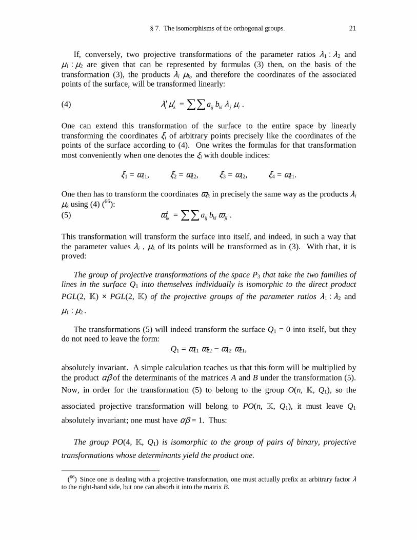
If, conversely, two projective transformations of the parameter ratios λ1 : λ2 and µ1 : µ2 are given that can be represented by formulas (3) then, on the basis of the transformation (3), the products λi µk, and therefore the coordinates of the associated points of the surface, will be transformed linearly: (4) i kλ µ′ ′ = ij kl j la b λ µ∑∑ .
One can extend this transformation of the surface to the entire space by linearly transforming the coordinates ξi of arbitrary points precisely like the coordinates of the points of the surface according to (4). One writes the formulas for that transformation most conveniently when one denotes the ξi with double indices:
ξ1 = ω11, ξ2 = ω22, ξ3 = ω12, ξ4 = ω21.
One then has to transform the coordinates ωik in precisely the same way as the products λi µk using (4) (66): (5) ikω′ = ij kl jla b ω∑∑ .
This transformation will transform the surface into itself, and indeed, in such a way that the parameter values λi , µk of its points will be transformed as in (3). With that, it is proved: The group of projective transformations of the space P3 that take the two families of lines in the surface Q1 into themselves individually is isomorphic to the direct product
PGL(2, K) × PGL(2, K) of the projective groups of the parameter ratios λ1 : λ2 and
µ1 : µ2 . The transformations (5) will indeed transform the surface Q1 = 0 into itself, but they do not need to leave the form:
Q1 = ω11 ω22 − ω12 ω21, absolutely invariant. A simple calculation teaches us that this form will be multiplied by the product αβ of the determinants of the matrices A and B under the transformation (5).
Now, in order for the transformation (5) to belong to the group O(n, K, Q1), so the
associated projective transformation will belong to PO(n, K, Q1), it must leave Q1
absolutely invariant; one must have αβ = 1. Thus:
The group PO(4, K, Q1) is isomorphic to the group of pairs of binary, projective
transformations whose determinants yield the product one.
(66) Since one is dealing with a projective transformation, one must actually prefix an arbitrary factor λ to the right-hand side, but one can absorb it into the matrix B.
22 I. Linear groups in arbitrary fields.
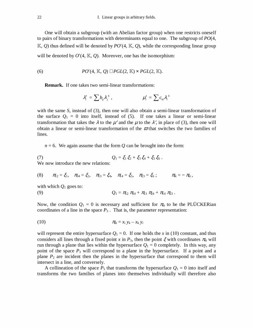
One will obtain a subgroup (with an Abelian factor group) when one restricts oneself to pairs of binary transformations with determinants equal to one. The subgroup of PO(4,
K, Q) thus defined will be denoted by PO′(4, K, Q), while the corresponding linear group
will be denoted by O′(4, K, Q). Moreover, one has the isomorphism:
(6) PO′(4, K, Q) ≅ PGL(2, K) × PGL(2, K).
Remark. If one takes two semi-linear transformations:
iλ′ = Sij jb λ∑ , iµ′ = S
kl lc λ∑
with the same S, instead of (3), then one will also obtain a semi-linear transformation of the surface Q1 = 0 into itself, instead of (5). If one takes a linear or semi-linear transformation that takes the λ to the µ′ and the µ to the λ′, in place of (3), then one will obtain a linear or semi-linear transformation of the ω that switches the two families of lines. n = 6. We again assume that the form Q can be brought into the form: (7) Q1 = ξ1 ξ2 + ξ3 ξ4 + ξ5 ξ6 . We now introduce the new relations: (8) π12 = ξ1, π34 = ξ2, π13 = ξ4, π14 = ξ5, π23 = ξ6 ; πik = − πki , with which Q1 goes to: (9) Q1 = π12 π34 + π13 π24 + π14 π23 . Now, the condition Q1 = 0 is necessary and sufficient for πik to be the PLÜCKERian coordinates of a line in the space P3 . That is, the parameter representation: (10) πik = xi yk – xk yi will represent the entire hypersurface Q1 = 0. If one holds the x in (10) constant, and thus considers all lines through a fixed point x in P3, then the point ξ with coordinates πik will run through a plane that lies within the hypersurface Q1 = 0 completely. In this way, any point of the space P3 will correspond to a plane in the hypersurface. If a point and a plane P2 are incident then the planes in the hypersurface that correspond to them will intersect in a line, and conversely. A collineation of the space P5 that transforms the hypersurface Q1 = 0 into itself and transforms the two families of planes into themselves individually will therefore also
§ 7. The isomorphisms of the orthogonal groups. 23
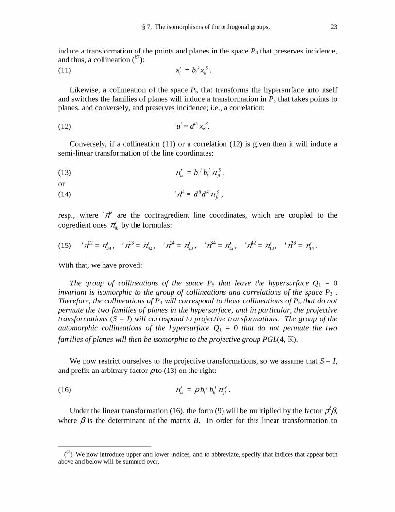
induce a transformation of the points and planes in the space P3 that preserves incidence, and thus, a collineation (67): (11) ix′ = k S
i kb x .
Likewise, a collineation of the space P5 that transforms the hypersurface into itself and switches the families of planes will induce a transformation in P3 that takes points to planes, and conversely, and preserves incidence; i.e., a correlation: (12) ′ui = dik xk
S. Conversely, if a collineation (11) or a correlation (12) is given then it will induce a semi-linear transformation of the line coordinates: (13) ikπ ′ = j l S
i k jlb b π ,
or (14) ′πik = ij kl S
jld d π ,
resp., where ′πik are the contragredient line coordinates, which are coupled to the cogredient ones ikπ ′ by the formulas:
(15) ′π12 = 34π ′ , ′π13 = 42π ′ , ′π14 = 23π ′ , ′π34 = 12π ′ , ′π42 = 13π ′ , ′π23 = 14π ′ .
With that, we have proved: The group of collineations of the space P5 that leave the hypersurface Q1 = 0 invariant is isomorphic to the group of collineations and correlations of the space P3 . Therefore, the collineations of P3 will correspond to those collineations of P5 that do not permute the two families of planes in the hypersurface, and in particular, the projective transformations (S = I) will correspond to projective transformations. The group of the automorphic collineations of the hypersurface Q1 = 0 that do not permute the two
families of planes will then be isomorphic to the projective group PGL(4, K).
We now restrict ourselves to the projective transformations, so we assume that S = I, and prefix an arbitrary factor ρ to (13) on the right: (16) ikπ ′ = j l S
i k jlb bρ π .
Under the linear transformation (16), the form (9) will be multiplied by the factor ρ2β, where β is the determinant of the matrix B. In order for this linear transformation to
(67) We now introduce upper and lower indices, and to abbreviate, specify that indices that appear both above and below will be summed over.
24 I. Linear groups in arbitrary fields.
belong to the group O(6, K, Q1), and thus, for the corresponding projective
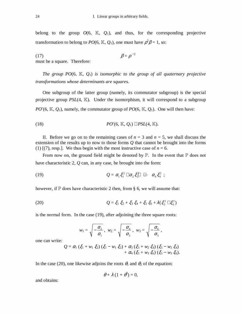
transformation to belong to PO(6, K, Q1), one must have ρ2β = 1, so:
(17) β = ρ −2 must be a square. Therefore:
The group PO(6, K, Q1) is isomorphic to the group of all quaternary projective
transformations whose determinants are squares. One subgroup of the latter group (namely, its commutator subgroup) is the special
projective group PSL(4, K). Under the isomorphism, it will correspond to a subgroup
PO′(6, K, Q1), namely, the commutator group of PO(6, K, Q1). One will then have:
(18) PO′(6, K, Q1) ≅ PSL(4, K).
II. Before we go on to the remaining cases of n = 3 and n = 5, we shall discuss the extension of the results up to now to those forms Q that cannot be brought into the forms (1) [(7), resp.]. We thus begin with the most instructive case of n = 6.
From now on, the ground field might be denoted by P. In the event that P does not
have characteristic 2, Q can, in any case, be brought into the form: (19) Q = 2 2 2
1 1 2 2 6 6α ξ α ξ α ξ+ + +⋯ ;
however, if P does have characteristic 2 then, from § 6, we will assume that:
(20) Q = ξ1 ξ2 + ξ3 ξ4 + ξ5 ξ6 +
2 25 6( )λ ξ ξ+
is the normal form. In the case (19), after adjoining the three square roots:
w1 = 2
1
αα
− , w2 = 4
3
αα
− , w3 = 6
5
αα
− ,
one can write: Q = α1 (ξ1 + w1 ξ2) (ξ1 − w1 ξ2) + α3 (ξ3 + w2 ξ4) (ξ5 − w2 ξ4) + α4 (ξ5 + w3 ξ6) (ξ5 − w3 ξ6). In the case (20), one likewise adjoins the roots θ1 and θ2 of the equation:
θ + λ (1 + θ2) = 0, and obtains:
§ 7. The isomorphisms of the orthogonal groups. 25
Q = ξ1 ξ2 + ξ3 ξ4 + λ (ξ5 − θ1 ξ6) (ξ5 − θ2 ξ6).
One thus always obtain a separable extension field K, in which the form Q can be
brought into the normal forms (7) or (9), for which the variables πik that enter into this
normal form will be linear functions of the original ξi with coefficients in K:
(21) πik = ike ν
νξ .
It is therefore remarkable that one will achieve a quadratic extension of K to the field
P in the case of Galois fields, as well as in the case of the field of real numbers.
All of the isomorphisms that were proved above will be true in the extension field K;
in particular, PO(6, K, Q) ≅ PO(6, K, Q1) is isomorphic to a subgroup of PGL(4, K). If
we now once more go from PO(6, K, Q) to the subgroup PO(6, P, Q) then we will have
to examine which subgroup of PGL(4, K) will correspond to it under the isomorphism.
A projective transformation T with coefficients in K belongs to the ground field P if
and only if it commutes with all automorphisms S of the GALOIS group G of K/P, or
more precisely, with all collineations (68): (22) iξ ′ = S
iξ (S in G).
This commutability is preserved under the isomorphic transition from the group of correlations and collineations of P3 . The correlations (22), which always leave the hypersurface Q = 0 invariant, might correspond to a collineation or a correlation CS of the space P3 . It then follows that:
Under the isomorphism, the group PO(6, P, Q) will correspond to the subgroup of
those transformations in PGL(4, K) whose determinants are squares and which commute
with all correlations (correlations CS, resp.) that belong to the substitutions S of the
GALOIS group of K/P.
(68) In order to prove this, one remarks that one must always be able to choose a matrix element of the projective transformation T that equals one. If T then commutes with the collineation (22) then all matrix
elements must admit the substitutions S, and therefore belong to P, since K is separable over P.
26 I. Linear groups in arbitrary fields.
These conditions will mean different things depending upon the nature of the CS . If CS is a correlation (12) then one can also characterize the collineations that commute with it as the ones that leave the form: (23) ik S
i kd x x
invariant, up to a factor.
Let P be − e.g. − the field of real numbers and let:
(24) Q = 2 2 2 2 2 2
1 2 3 4 5 6ξ ξ ξ ξ ξ ξ+ + + + + .
The substitution (21), which brings Q into the form (9), then reads like: π12 = ξ1 + i ξ2, π13 = ξ3 + i ξ4 , π14 = ξ5 + i ξ6 , π34 = ξ1 − i ξ2, π42 = ξ3 − i ξ4 , π23 = ξ5 − i ξ6 . Now, the collineation (22) takes π12 to 34
Sπ , π13 to 42Sπ , π14 to 23
Sπ , and conversely,
where S is the transition to the complex conjugate. Under the isomorphism, it will correspond to the correlation:
′ui = xi S,
from which, one can define the HERMITIAN form: (25) S
i jx x∑ = i ix x∑ .
If a real projective transformation leaves this form invariant, up to a factor, then that factor must be positive, since the form (25) is positive-definite. Therefore, one can also choose the factor to be equal to one. We then have the isomorphism:
(26) PO1(6, P) ≅ PU(4, K).
The same argument will always be true with small modifications when the form Q has one of the following two forms: (27) Q2 = ϕ(ξ1, ξ2) + ϕ(ξ3, ξ4) + ϕ(ξ5, ξ6), (28) Q3 = ϕ(ξ1, ξ2) + ξ3 ξ4 + ξ5 ξ6 ,
where ϕ is a quadratic form that is indecomposable in P. In the first case (27), the
associated form (23) has the form (25), while in the second case (28), it has the form: (29) 1 2 2 1 4 3 3 4x x x x x x x x− + − .
One will thus always obtain a unitary group for Q2, and a hyper-Abelian group for Q3 . If one goes to those subgroups PSU (PSH, resp.) whose elements leave the form (25) [(29),
§ 7. The isomorphisms of the orthogonal groups. 27
resp.] absolutely invariant and have the determinant one then under the isomorphism it will also correspond to a subgroup PO′ with Abelian factor groups:
(30) PO′(6, P, Q2) ≅ PSU(4, K),
(31) PO′(6, P, Q3) ≅ PSH(4, K).
If K is a GALOIS field then, from § 5, the groups PSU and PSH on the right-hand
side will be isomorphic to each other. The forms Q1 and Q2 (or also Q1 and Q3) with discriminants – 1 and – v will also already exhaust all types of quadratic forms over a Galois field GF(q). The same will also be true for complete fields of characteristic 2,
where Q1 and Q2 belong to the groups J0 and Jλ , resp. If P is the field of real numbers
then the forms Q2 and Q3 will have the indices of inertia 1 and 0, resp., while the form Q1 will have the index 3. A form of index of inertia 1 can be treated by the same method: One obtains the group of projective transformations that commute with an anti-collineation of the form:
1x′ = 4x , 2x′ = − 3x , 3x′ = + 2x , 4x′ = − 1x .
From STUDY (63), one can represent these transformations very elegantly by quaternion matrices. The case n = 4 is completely analogous. Here, as well, by the introduction of new variables:
ωik = ikd ννξ ,
one brings the form Q into the form:
Q = ω11ω22 – ω12 ω21 , then looks for a semi-linear transformation CS of the λ and µ that corresponds to the collineation:
νξ ′ = ξvS,
and finally defines the group of pairs of projective transformations of the parameter ratios λ1 : λ2 and µ1 : µ2 that commute will CS . In addition to (1), two forms of the form Q come into consideration: (32) Q2 = ξ1 ξ2 + ϕ(ξ3, ξ4), (33) Q3 = ϕ(ξ1, ξ2) + ϕ(ξ3, ξ4). For the field of real numbers, Q1, Q2, Q3 will be typical forms with indices of inertia 2, 1, and 0, resp. For the Galois field GF(q), Q1 and Q2 will already exhaust the possible cases (discriminants square or not, resp.). In the case of the form Q2, CS will be the transformation:
28 I. Linear groups in arbitrary fields.
1 1
2 2
,
,
S
S
λ µλ µ
′ = ′ =
1 1
2 2
,
.
S
S
µ λµ λ
′ = ′ =
In order for a pair of binary, projective transformations A, B to commute with CS, one must have:
B = ρ AS
for their matrices, while A remains arbitrary. Instead of the direct product PGL(2, K) ×
PGL(2, K) in the isomorphism that was mentioned at the beginning of this paragraph, one
will obtain only the one group PGL(2, K). The subgroup PO(4, P, Q2) will be
isomorphic to the group of those transformations in PGL(2, K) whose determinants α
have the property that:
α αS = ρ−2 = square in K.
This condition is fulfilled automatically in the case of the Galois field or the field of real numbers. Thus, one will have the isomorphism:
(34) PO(4, P, Q2) ≅ PGL(2, K)
in these two cases. In the real case, the group on the left-hand side is essentially the Lorentz group of the special theory of relativity. In the case Q3, CS will be the transformation:
1 2
2 1
,
,
S
S
λ λλ λ
′ = ′ = −
1 2
2 2
,
.
S
S
µ µµ µ
′ = ′ = −
The condition that the pair (A, B) should commute with this transformation will now yield two separate conditions for A and B. The condition for A is that (λ2
S, − λ1S) should
transform like λ1, λ2, up to a factor, or that the form: (35) λ1 λ2
S + λ2 λ1S
should remain invariant, up to a factor; the condition for B reads correspondingly. We are thus dealing with two extended unitary groups. Under the transition to the restricted unitary group, one will obtain a subgroup with an Abelian factor group:
(36) PO′(4, P, Q2) ≅ PSU(2, P, K) × PSU(2, P, K).
One can also write the unitary transformation in this case in the form:
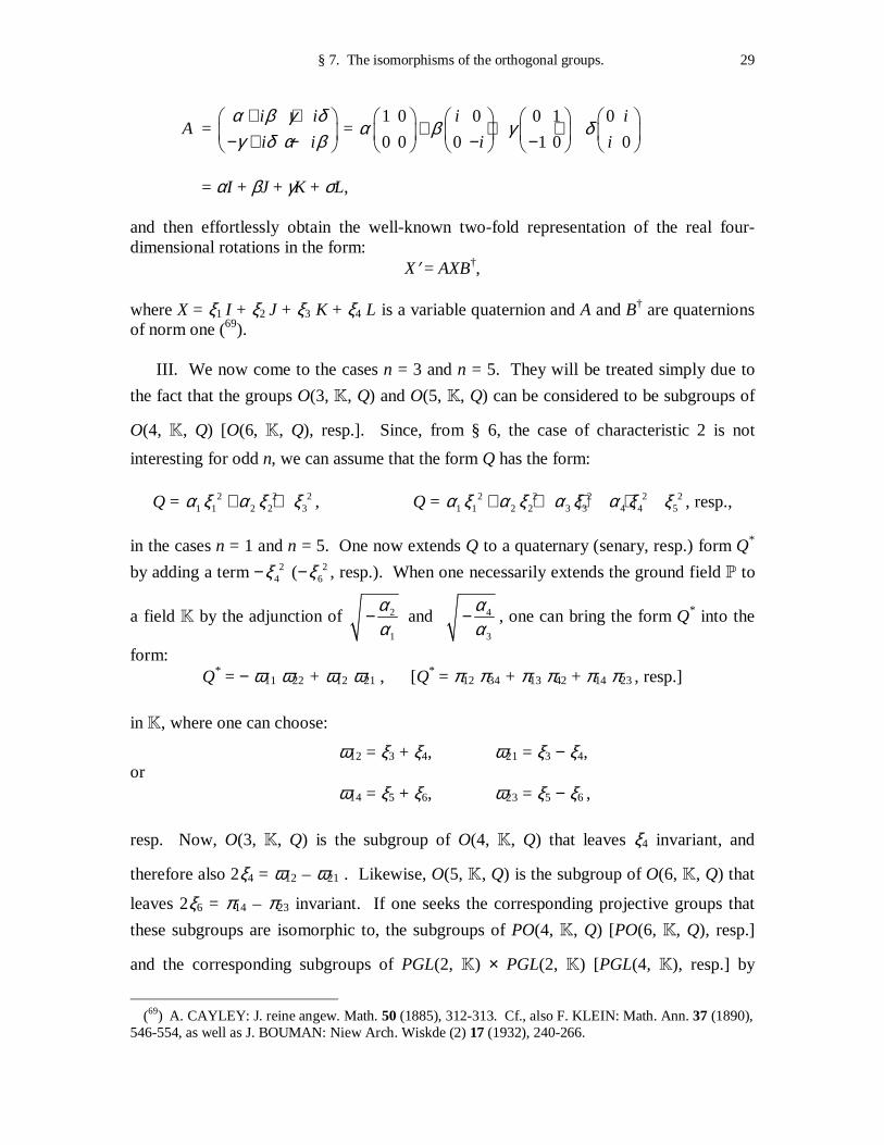
§ 7. The isomorphisms of the orthogonal groups. 29
A = i i
i i
α β γ δγ δ α β
+ + − + −
= 1 0 0 0 1 0
0 0 0 1 0 0
i i
i iα β γ δ
+ + + − −
= αI + βJ + γK + σL, and then effortlessly obtain the well-known two-fold representation of the real four-dimensional rotations in the form:
X′ = AXB†,
where X = ξ1 I + ξ2 J + ξ3 K + ξ4 L is a variable quaternion and A and B† are quaternions of norm one (69). III. We now come to the cases n = 3 and n = 5. They will be treated simply due to
the fact that the groups O(3, K, Q) and O(5, K, Q) can be considered to be subgroups of
O(4, K, Q) [O(6, K, Q), resp.]. Since, from § 6, the case of characteristic 2 is not
interesting for odd n, we can assume that the form Q has the form:
Q = 2 2 21 1 2 2 3α ξ α ξ ξ+ + , Q = 2 2 2 2 2
1 1 2 2 3 3 4 4 5α ξ α ξ α ξ α ξ ξ+ + + + , resp.,
in the cases n = 1 and n = 5. One now extends Q to a quaternary (senary, resp.) form Q*
by adding a term − 24ξ (− 2
6ξ , resp.). When one necessarily extends the ground field P to
a field K by the adjunction of 2
1
αα
− and 4
3
αα
− , one can bring the form Q* into the
form: Q* = − ω11 ω22 + ω12 ω21 , [Q* = π12 π34 + π13 π42 + π14 π23 , resp.]
in K, where one can choose:
ω12 = ξ3 + ξ4, ω21 = ξ3 − ξ4, or ω14 = ξ5 + ξ6, ω23 = ξ5 − ξ6 ,
resp. Now, O(3, K, Q) is the subgroup of O(4, K, Q) that leaves ξ4 invariant, and
therefore also 2ξ4 = ω12 – ω21 . Likewise, O(5, K, Q) is the subgroup of O(6, K, Q) that
leaves 2ξ6 = π14 – π23 invariant. If one seeks the corresponding projective groups that
these subgroups are isomorphic to, the subgroups of PO(4, K, Q) [PO(6, K, Q), resp.]
and the corresponding subgroups of PGL(2, K) × PGL(2, K) [PGL(4, K), resp.] by
(69) A. CAYLEY: J. reine angew. Math. 50 (1885), 312-313. Cf., also F. KLEIN: Math. Ann. 37 (1890), 546-554, as well as J. BOUMAN: Niew Arch. Wiskde (2) 17 (1932), 240-266.
30 I. Linear groups in arbitrary fields.
means of the aforementioned isomorphism, then one will ultimately find, in the case n = 3, the group of those pairs of projective transformations of λ1 : λ2 and µ1 : µ2 that leave the form: (38) λ1 µ2 − λ2 µ1 invariant, up to a factor, and in the case n = 5, likewise that quaternary projective group that leave the form: (39) (x1 y4 – x4 y1) + (x3 y2 – x2 y3), up to a factor. The invariance of the form (38) says that µ1 : µ2 will be transformed in precisely the same way as λ1 : λ2 : one will then have the isomorphism:
(40) O(3, K, Q) ≅ PGL(2, K).
One can also infer this directly from the parametric representation of the conic section Q = 0. The projective transformations of the conic section into itself will, in fact, induce fractional linear parameter transformations, and conversely. The condition for the invariance of (39), up to a factor, defines an extension of the complex group. If one restricts oneself to those transformations that leave the form (39) absolutely invariant then one will obtain a normal subgroup with an Abelian factor group:
(41) O′(5, K, Q) ≅ PC(4, K).
The reversion of the super-field K to a sub-field P can, when necessary, be performed
by the process that was explained in II for n = 4 and n = 6. In the case of the Galois field, the transition is not necessary, just as in the case of the real “group of hyperbolic motions”:
Q = − 2 2 21 2 3ξ ξ ξ+ + .
In the case of the field of real numbers and the form:
Q = 2 2 21 2 3ξ ξ ξ+ + ,
one will obtain the well-known isomorphism (cf., the beginning of this paragraph):
(42) O1(3, K) ≅ PSU(2, P, K).
§ 8. Linear groups in complex number fields. 31
§ 8. Linear groups in complex number fields. Reducible and irreducible, primitive, imprimitive, and monomial groups.
The groups of linear substitutions with complex number coefficients, which will be called linear groups in what follows, are somewhat easier to survey when one restricts oneself to closed groups – i.e., to groups that include all of their accumulation elements – as long as they are not singular. From a theorem of J. V. NEUMANN (70), any closed linear group G behaves as follows: G contains an r-parameter continuous (LIE) subgroup
H, which is a normal subgroup of G, and the factor classes of H are isolated from each
other – i.e., none of them contain accumulation elements of the union of the other ones. This theorem is a special case of a theorem on closed subgroups of LIE groups that E. CARTAN (71) has proved very simply. The two extreme cases for closed, linear groups are thus: The continuous groups, where H = G and the discrete (or discontinuous) ones,
where H consists of only the unity element I. A group is then called discrete when the
unity element (and thus, also any other group element) is not an accumulation element of other group elements (72). The structure of continuous groups will be examined in the LIE theory, to which another booklet in this series will be directed. We thus content ourselves here with the proof that an r-parameter continuous linear group will be determined by r linearly-independent matrices A1, …, Ar – viz., the matrices of the “infinitesimal generators” – in such a way that the r one-parameter subgroups that are defined by the matrices itAe (i = 1, 2, …, r), where t runs through all real numbers, collectively generate the r-parameter group. Any group element in the neighborhood of one can be represented “canonically” by:
1 1 r rt A t Ae + +⋯ .
Therefore, eA will be defined by the exponential series. The matrices A1, …, Ar must fulfill the relations:
Ai Ak – Ak Ai = lik lc A∑ ,
where the real constants likc depend upon only the “structure” group – i.e., they will be
the same for two groups that are “continuously isomorphic in the small (71).” Especially important are the semi-simple continuous groups; i.e., the ones that contain no solvable, continuous, normal subgroup. E. CARTAN (73) has enumerated these groups completely, and their representations by linear transformations are also all known, in principle, (74). (70) J. V. NEUMANN, Math. Z. 30 (1929), 3-42. (71) E. CARTAN: Mém. Sci. math. 42 (1930), in particular, § 27. (72) It only makes sense to speak of a discrete group when a topology is defined on the group (which is indeed the case for linear groups). There is no meaning to calling an abstract group discrete or discontinuous. (73) E. CARTAN: Thése. Paris 1894 (2nd ed., Paris, 1933) – Ann. École norm. 31 (1914), 263-355. Cf., also VAN DER WAERDEN: Math. Z. 37 (1933), 446-462 and W. LANDHERR, Bull. Soc. Math. Semin. Hamburg. Univ. 11 (1934), 41-64. (74) E. CARTAN: Bull. Soc. Math. France 41 (1913), 53-96. − J. Math. pures appl. (6) 10 (1914), 149-186. – H. WEYL: Math. Z. 23 (1925), 271-309; 24 (1925), 328-395.
32 I. Linear groups in arbitrary fields.
A discrete linear group with restricted matrix elements is obviously finite; in particular, a discrete group of unitary transformations is therefore always finite. The following converse of this theorem is true: Any finite linear group can leave a positive-definite HERMITIAN form ∑ ∑ αik ξi ξk invariant. In order to prove this, like R. L. MOORE (75), one needs only to subject the form ∑ ξi ξi to all transformations of the group and define the sum. The same method of proof is valid when one, like HURWITZ (76), replaces the summation with a suitable integration, and also for compact, continuous groups − indeed for arbitrary compact groups, according to HAAR (76a). More generally, one has: If the matrix elements of a linear group G are uniformly restricted then G will possess an invariant positive
HERMITIAN form. H. AUERBACH (77) gave a direct proof of this. One can, however, also derive the theorem from the theorem above on the structure of the closed groups when one defines the (compact) closed hull of G, which possesses a continuous normal
subgroup H with mutually isolated cosets, hence, only finitely many of them, due to
compactness. MOORE’s proof above can be duplicated by integrating over the subgroup H and summing over the cosets.
Since one can easily transform any positive-definite HERMITIAN form into the form:
1
n
i ii
ξ ξ=∑
by introducing new coordinates (the proof is completely analogous to the one that is known for quadratic forms), from the discussion of finite (or more generally restricted) linear groups, one can always restrict oneself to groups of unitary transformations. For finite groups, one can replace the HERMITE form with the corresponding quadratic form, and thus assume that the transformations of the group are orthogonal. A linear group is called reducible (or in a terminology that has justifiably fallen out of use: intransitive) when it leaves a proper subspace Em of the vector space En (0 < m < n) invariant. MASCHKE’s Theorem follows immediately from the existence of an invariant HERMITIAN form (78): If a finite (or, more generally, a restricted) linear group is reducible then the vector space En can be decomposed into two invariant subspace: En = Em + En−m (79). En−m is, in fact, the space that is “totally perpendicular” to Em for the metric that is determined by the HERMITIAN form. We shall return to the general properties of reducible and irreducible linear groups (in arbitrary fields) in § 11 – 15. According to E. CARTAN (80), an irreducible continuous linear group is either semi-simple or the product of a semi-simple normal subgroup with an Abelian continuous group that consists of multiples λI of the identity. Since one
(75) R. L. MOORE: Math. Ann. 50 (1898), 213-214. There is further literature in this paper. (76) A. HURWITZ: Nachr. Ges. Wiss. Göttingen 1897, 71-90, Cf., also WEYL (74). (76a) A. HAAR: Ann. of Math. II, pp. 34 (1933), 147-169. (77) H. AUERBACH: C. R. Acad. Sci., Paris 195 (1932), 1367. (78) H. MASCHKE, Math. Ann. 52 (1899), 363-368. (79) + means the direct sum (in the sense of additive groups). (80) E. CARTAN: Ann. Écol. norm. 26 (1909), 147-148 – Bull. Soc. Math. France 41 (1913), 53-96.
§ 8. Linear groups in complex number fields. 33
knows the semi-simple linear groups, in principle (see above), the irreducible continuous groups will also be known, in principle. A linear group is called imprimitive when there is a decomposition of the space En into subspaces Eh + Ek + … + El that are only permuted with each other by the group; otherwise, it will be called primitive. If the group G is irreducible, but imprimitive, then
h = k = … = l. In particular, if h = k = … = l = 1 then the group will be called monomial. An imprimitive group G possesses a reducible normal subgroup H that leaves the
spaces Eh , Ek , …, El individually invariant. G / H is isomorphic to a permutation group.
If G is monomial then H will be Abelian. Conversely, if a linear group G possesses any
Abelian normal subgroup that does not consist of just λI then G will be imprimitive. The
proof is implied easily from the fact that one can bring all of the transformations of H
into diagonal form simultaneously. It then follows: A linear group is imprimitive when it includes a finite, Abelian, normal subgroup that does not contain the center. H. F. BLICHFELDT (81) and K. SHODA (82) have presented further theorems on imprimitive groups and their normal subgroup. It follows easily from the criterion for imprimitivity that was formulated that a linear group of prime-power order is always monomial (83); likewise, any two-level (i.e., meta-Abelian) linear group (84), and in particular, any linear group of quadratic order, is monomial (85). The method of proof is always the same: The trivial Abelian case is omitted. In the non-Abelian case, there exists an Abelian normal subgroup that does not contain the center. Imprimitivity follows from that, and thus, the existence of an invariant decomposition En = Eh + Ek + … If one then restricts oneself to the subgroup that leaves Eh invariant then it will again be imprimitive in Eh, on the same basis; one can then further decompose Eh, and correspondingly, Ek, …, until one has obtained an invariant decomposition into one-dimensional subspaces. According to C. JORDAN (86), any finite linear group G possesses an Abelian normal
subgroup H whose index i does not exceed a limit that depends upon only n. The order
of G is then equal to the order h of H, multiplied by the restricted number i. In particular,
if G is primitive then, from the theorem above, H will consist of only multiples of the
identity, so the order of the projective group that corresponds to G will be restricted
(namely, it will be equal to i). L. BIEBERBACH (87) has given a simple proof of the aforementioned theorem of JORDAN with explicit assumed limits that was simplified by G. FROBENIUS (88) and sharpened by A. SPEISER (89). The cited proofs all rest upon the fact that two (81) H. F. BLICHFELDT: Trans. Amer. Math. Soc. 4 (1903), 387-397; 5 (1904), 310-325. (82) K. SHODA: J. Fac. Sci. Univ. Tokyo 2 (1931), 180-209. (83) See footnote (81). Cf., also MILLER-BLICHFELDT-DICKSON: Theory and application of finite groups, New York, 1916. (84) K. TAKETA: Proc. Imp. Acad. Tokyo 6 (1930), 31-33. (85) W. BURNSIDE: Messenger Math. (2) 35 (1906), 46-50. (86) C. JORDAN: J. reine angew. Math. 84 (1878), 89-213. (87) L. BIEBERBACH: S.-B. preuss. Akad. Wiss. (1911), 231-240. (88) G. FROBENIUS: S.-B. preuss. Akad. Wiss (1911), 241-248. (89) A. SPEISER: Theorie der Gruppen von endlicher Ordnung, 2nd ed., Berlin, 1927, § 68.
34 I. Linear groups in arbitrary fields.
substitutions in a finite linear group that are sufficiently close to the identity will necessarily commute. FROBENIUS (90) gave the sharpest definition of “sufficiently close”: It suffices that the characteristic roots of the one substitution do not occupy all of one-sixth of the unit circle, and those of the other substitution do no occupy all of one-half of it. H. F. BLICHFELDT (91) has presented sharper limits for the order of a primitive, unimodular, linear group and the prime-powers that come about for them. His method rests upon the arithmetic discussion of an algebraic equation that couples the traces of the transformations Σ, Σ Τ, Σ Τ2, …, Σ Τn−1, and Σ Τr (r > n – 1) with each other and with the characteristic roots of Τ, if Σ and Τ are arbitrary elements of the group. This method also produces another proof of JORDAN’s theorem above. The theorems of MASCHKE and JORDAN were adapted to infinite groups of periodic linear substitutions (i.e., linear substitutions of finite order) by I. SCHUR (92). On these groups, cf., furthermore W. BURNSIDE: Proc. London Mat. Soc. (2) 3 (1905), 435-440. For another generalization of the finite linear groups, see A. LOEWY: Math. Ann. 64 (1907), 264-272. I. SCHUR (93) has proved, by arithmetic methods, that the order of a finite group of given degree is restricted, as long as one is given which part of the circle that the traces of the group elements belong to.
§ 9. Finite, linear groups of given degree.
For the presentation of the finite, linear groups of given degree (i.e., given dimension number) over the field of complex numbers, one restricts oneself to linear transformations with determinant 1 (or possibly ± 1), for the sake of convenience. We will tacitly make this restriction in what follows. Moreover, following § 8, the transformations will all be assumed to be unitary (orthogonal, resp., for real groups). A projective group G′ belongs to any linear group G: namely, the factor group of G
with respect to the subgroup of transformations λI in G. The presentation of linear
groups of a given degree mostly precedes the presentation of the associated projective groups. For each such projective group G′, there is a greatest associated linear group G
that consists of all linear transformations with determinant 1, whose associated projective transformations lie in G′. This group is mapped to G′ in an n-to-one homomorphic, since
each projective transformation corresponds to n linear ones with determinant 1. All linear groups that correspond to the same projective group G′ are included in this one
group G.
(90) S.-B. preuss. Akad. Wiss. (1911), 373-378. (91) H. F. BLICHFELDT: Trans. Amer. Math. Soc. 4 (1903), 387-397; 5 (1904), 310-325; 12 (1911), 39-42. (92) I. SCHUR, S.-B. preuss. Akad. Wiss. (1911), 619-627. (93) I. SCHUR: S.-B. preuss. Akad. Wiss (1905), 77-91.
§ 9. Finite, linear groups of given degree. 35
F. Klein (94) has determined the finite binary projective groups by converting the binary projective groups into ternary real rotation groups by means of the isomorphism
O(3; P) ≅ PU(2, K) that was discussed in § 7. He then found the well-known types:
cyclic groups, dihedral groups, tetrahedral groups, octahedral groups, icosahedral groups. H. H. MITCHELL (95) gave a very simple direct derivation of these types. The previously-remarked binary, linear groups of double order belong to these projective groups. Only the cyclic and dihedral groups also belong to linear groups of the same order. There are no other finite, binary, linear groups with determinant 1. The finite, ternary, projective groups were presented incompletely by C. JORDAN (96) and H. VALENTINER (97), and completely by H. F. BLICHFELDT (98) [cf., also H. H. MITCHELL (95)]. Since the imprimitive groups are either reducible or monomial, and thus relatively easy to find, it will suffice to give the primitive groups. They are: 1. The projective, ternary icosahedral group G60, which corresponds to the real, orthogonal, icosahedral group. 2. The group that JORDAN called the “HESSIAN group” G216, which takes the inflection point configuration of a plane curve of order three to itself (99). 3. A normal divisor G72 of G216 (
99). 4. A normal divisor G36 of G216 (
99). 5. A group G168 that is isomorphic to PSL(2, 7) and was discovered by KLEIN (100). 6. A group that was discovered by VALENTINER (97) and then WIMAN (101) that is isomorphic to the alternating subgroup A6 of G360 .
These projective groups correspond naturally to linear groups of three-fold order that are the 3-homomorphic images of them. Only the groups G168 and G60 have 1-isomorphic linear groups. E. Goursat (102) has determined the finite, real (orthogonal), quaternary, projective group. On the basis of the isomorphism:
PO(4, P) ≅ PU(2, K) × PU(2, K)
that was discussed in § 7, the determination of the finite, real, quaternary groups comes down to the determination of all groups of pairs of binary, unitary substitutions. GOURSAT has also given all extensions of the groups found to orthogonal substitutions
(94) F. KLEIN: Math. Ann. 9 (1876), 183-208. (95) H. H. MITCHELL: Trans. Amer. Math. Soc. 12 (1911), 208-211. (96) C. JORDAN: J. reine angew. Math. 84 (1878), 89-215. (97) H. VALENTINER: Skr. Widensk.-Selsk. Kopenhagen (6) 5 (1889), 64-235. (98) H. F. BLICHFELDT: Trans. Amer. Math. Soc. 5 (1904), 321-325 – Math. Ann. 63 (1907), 552-572. (99) For a more precise discussion of these groups, we refer to the encyclopedia article of A. WIMAN: “Endliche Gruppen linearer Substitutionen,” Enc. math. Wiss. IB, 3f. Cf., also K. RÖSSLER: Čas. pést. Mat. a Fys. 60 (1931), 166-172. (100) F. KLEIN: Math. Ann. 14 (1879), 438. (101) A. WIMAN: Math. Ann. 47 (1896), 531-556. (102) E. GOURSAT: Ann. École norm. (3) 6 (1889), 9-102. Cf., also G. BAGNERA: Rend. Circ. mat. Palermo 15 (1901), 161-309.
36 I. Linear groups in arbitrary fields.
of determinant – 1. W. THRELFALL and H. SEIFERT (103) have determined the orthogonal groups that belong to the orthogonal projective groups with determinant 1 that were found by GOURSAT. Among these groups, one naturally also finds groups of deck motions of the regular polytopes in R4 that were exhibited by various authors (104) since GOURSAT up to recently. H. F. BLICHFELDT (105) has presented the complex, quaternary, primitive groups by his arithmetic methods that were already mentioned in § 8. G. BAGNERA and H. H. MITCHELL (106) repeated the determination by geometric methods. Some of the more remarkable of these groups are three simple groups of orders 168, 2520, and 25,920 (107), a group of order 16,720 that was discovered by KLEIN (99) that has normal subgroups of order 16 ⋅⋅⋅⋅ 360 and 16, as well as two groups that are isomorphic to S6 (A7, resp.) and
their subgroups (108) that are isomorphic to A6, S5, and A5 . W. BURNSIDE (109) and H.
H. MITCHELL (110) have given a series of remarkable linear groups in more than four variables. For the groups of the regular polytopes (simplexes and hyperoctahedra) in n > 4 dimensions, see (104) and (111). One can determine the solvable linear groups of prime degree following BURNSIDE (111a). One finds further theorems on the structure of finite groups of prime degree in K. SHODA (82).
§ 10. Infinite, discrete groups of fractional linear transformations; in particular, discrete groups of motions.
For the older literature on this topic, we refer, once and for all, to the encyclopedia article of FRICKE on automorphic functions (112). A group G of one-to-one, continuous transformations in a spatial region D is called
properly discontinuous when each point P of a domain D possesses a neighborhood U that has only finitely many points in common with the image neighborhoods SU (S comes
(103) W. THRELFALL and H. SEIFERT: Math. Ann. 104 (1931), 1-70. (104) Of the recent ones, let us mention only: D. E. LITTLEWOOD: Proc. London Math. Soc. 32 (1930), 10-20. – J. A. TODD: Proc. Cambridge Philos. Soc. 27 (1931), 212-231. (105) H. F. BLICHFELDT: Trans. Amer. Math. Soc. 6 (1905), 230-236. – Math. Ann. 60 (1905), 204-231. (106) G. BAGNERA: Rend. Circ. mat. Palermo 19 (19105), 1-56. – H. H. MITCHELL: Trans. Amer. Math. Soc. 14 (1913), 123-142. (107) Cf., A. WITTING: Diss. Göttingen, 1887. See also the encyclopedia article IB, 3f, of A. WIMAN, no. 23. (108) See H. MASCHKE: Math. Ann. 51 (1899), 253-298, as well A. WIMAN: Math. Ann. 52 (1899), 243-270. (109) W. BURNSIDE: Proc. London Math. Soc. (2) 10 (1911), 284-308. (110) H. H. MITCHELL: Trans. Amer. Math. Soc. 16 (1914), 1-12. (111) G. DE B. ROBERTSON: Proc. Cambridge Philos. Soc. 26 (1930), 94-98. – D. M. Y. SOMMERVILLE: Proc. London Math. Soc. (2) 35 (1933), 101-115. (111a) W. BURNSIDE: Acta math. 27 (1903), 217-224. (112) R. FRICKE: Enc. math. Wiss. IIB, 4 (1913).
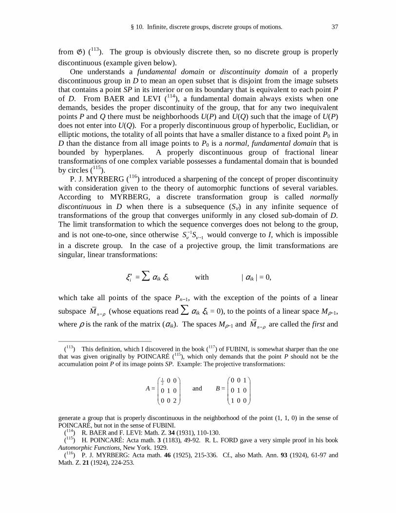
§ 10. Infinite, discrete groups, discrete groups of motions. 37
from G) (113). The group is obviously discrete then, so no discrete group is properly
discontinuous (example given below). One understands a fundamental domain or discontinuity domain of a properly discontinuous group in D to mean an open subset that is disjoint from the image subsets that contains a point SP in its interior or on its boundary that is equivalent to each point P of D. From BAER and LEVI (114), a fundamental domain always exists when one demands, besides the proper discontinuity of the group, that for any two inequivalent points P and Q there must be neighborhoods U(P) and U(Q) such that the image of U(P) does not enter into U(Q). For a properly discontinuous group of hyperbolic, Euclidian, or elliptic motions, the totality of all points that have a smaller distance to a fixed point P0 in D than the distance from all image points to P0 is a normal, fundamental domain that is bounded by hyperplanes. A properly discontinuous group of fractional linear transformations of one complex variable possesses a fundamental domain that is bounded by circles (115). P. J. MYRBERG (116) introduced a sharpening of the concept of proper discontinuity with consideration given to the theory of automorphic functions of several variables. According to MYRBERG, a discrete transformation group is called normally discontinuous in D when there is a subsequence (Sν) in any infinite sequence of transformations of the group that converges uniformly in any closed sub-domain of D. The limit transformation to which the sequence converges does not belong to the group, and is not one-to-one, since otherwise 1
1S Sν ν−
− would converge to I, which is impossible
in a discrete group. In the case of a projective group, the limit transformations are singular, linear transformations:
iξ ′ = ∑ αik ξk with | αik | = 0,
which take all points of the space Pn−1, with the exception of the points of a linear
subspace nM ρ− (whose equations read ∑ αik ξk = 0), to the points of a linear space Mρ−1,
where ρ is the rank of the matrix (αik). The spaces Mρ−1 and nM ρ− are called the first and
(113) This definition, which I discovered in the book (117) of FUBINI, is somewhat sharper than the one that was given originally by POINCARÉ (115), which only demands that the point P should not be the accumulation point P of its image points SP. Example: The projective transformations:
A =
12 0 0
0 1 0
0 0 2
and B = 0 0 1
0 1 0
1 0 0
generate a group that is properly discontinuous in the neighborhood of the point (1, 1, 0) in the sense of POINCARÉ, but not in the sense of FUBINI. (114) R. BAER and F. LEVI: Math. Z. 34 (1931), 110-130. (115) H. POINCARÉ: Acta math. 3 (1183), 49-92. R. L. FORD gave a very simple proof in his book Automorphic Functions, New York. 1929. (116) P. J. MYRBERG: Acta math. 46 (1925), 215-336. Cf., also Math. Ann. 93 (1924), 61-97 and Math. Z. 21 (1924), 224-253.
38 I. Linear groups in arbitrary fields.
second limit element of the sequence (Sν), respectively. If the inverse sequence 1( )Sν−
again converges then its first limit element will be contained in nM ρ− , while its second
limit element will be subsumed by Mρ−1 . A discrete group of projective transformations is normally discontinuous in D when the second limit element nM ρ− of the convergent sequence (Sν) contains no point of D
outside the group. The domain of normal discontinuity of a discrete, projective group is then the totality of all points that belong to no nM ρ− (and, as a result, also to no Mρ−1).
The concept of normal discontinuity will coincide with that of proper discontinuity for n = 2, and thus for the case of fractional linear substitutions of one real or complex variable. In the general case, proper discontinuity will follow from the normal kind, but not the converse: The domain D of normal discontinuity is a subset of the domain of proper discontinuity. Proof: A point P of D has a neighborhood U, whose closed hull still belongs to D. If infinitely many images SU still had points in common with U then one could select a convergent sequence (Sν) from the S. Since U lies separate from the second limit element nM ρ− of this sequence, the image sets SνU will gravitate towards
Mρ−1 ; thus, not all SνU can have points in common with U. One proves in a completely analogous way that the BAER-LEVI condition that was cited above for the existence of a fundamental domain under normal discontinuous groups is always fulfilled. According to MYRBERG (116), a discrete projective group, among others, is normally discontinuous in a domain D when D remains invariant under the group and has no points in common with a system of n hypersurfaces that do not go through a point. The latter condition is then the case, in particular, when the invariant domain D lies entirely are finite points. The real, discrete, projective groups that leave invariant an indefinite, quadratic form whose index of inertia is 1 or 2 possess a domain of normal discontinuity in real Pn−1 . In particular, a discrete group of hyperbolic motions is normally discontinuous in the entire interior of any quadratic fundamental surface (117). Likewise, the complex, discrete, projective groups that leave a HERMITIAN form:
H = 1 1 2 2 1 1n n n nξ ξ ξ ξ ξ ξ ξ ξ− −+ + + −⋯
invariant in the domain H < 0 (and also in the domain H > 0 for n = 2) will be normally discontinuous. One calls these groups Fuchsian for n = 2 and for hyper-Fuchsian for n > 2. One finds further examples of normally discontinuous groups − in particular, the ones that leave no domain D invariant − in MYRBERG (116). I add that the discrete groups of real, Euclidian motions:
0
0 0
,
,i ik k iξ α ξ γ ξ
ξ ξ′ = +
′ =
∑ (αik) orthogonal
(117) G. FUBINI: Introduzione alla teoria dei gruppi discontinui e delle funzioni automorfe, Pisa, 1908.
§ 10. Infinite, discrete groups, discrete groups of motions. 39
are all normally discontinuous in the domain of finite points (ξ0 ≠ 0). In fact, a convergent sequence of such motions will always converge for a non-singular motion, unless some γi increases to infinity, in which case, after multiplying by a 1
iγ − that
converges to zero strongly, a limit transformation:
0
0 0i iξ β ξ
ξ′ =
′ =
will come about whose limit elements Mρ−1 and nM ρ− both lie at infinity.
A real, linear transformation of ξ1, …, ξn induces a linear transformation of the coefficients z1, …, zN of a quadratic form in the x. Likewise, a complex, linear transformation of ξ1, …, ξn induces a real, linear transformation of the real and imaginary parts of the coefficients of a HERMITIAN form, which we again denote by z1, …, zN . Therefore, those pairs of linear transformations that differ by only a factor λ will again induce similar pairs of transformations of z1, …, zN ; one can then say that the real (complex, resp.) projective transformations of a space Pn−1 into a space PN−1 induce real projective transformations in both cases. There is a sub-domain D in PN−1 whose points belong to the definite forms. This sub-domain is always connected, and will be transformed into itself by all of the transformations considered. One now has: Under the association above, a discrete group of real (complex, resp.) projective transformations corresponds to a discrete group of real, projective transformations of PN−1, which is normally discontinuous in the domain D (117). In particular, for n = 2, the fractional linear transformations of one complex variable ξ = ξ1 : ξ2 :
(1) 1 1 2
2 1 2
,
,
ξ αξ βξξ γξ δξ
′ = + ′ = +
or ζ′ = αζ βγζ δ
++
correspond to real transformations of the space P3 whose coordinates are the real and imaginary parts of z1, z2, z3, z4 of the coefficients of the HERMITIAN form:
1 1 1 2 3 1 2 2 3 2 1 4 2 2( ) ( )z z iz z iz zξ ξ ξ ξ ξ ξ ξ ξ+ + + − + .
The definite forms are characterized by:
Q = 2 22 3z z+ − z1 z4 < 0;
our transformations then leave the interior of the surface Q = 0 invariant, and are then hyperbolic motions. Each discrete group of ζ-substitutions (1) corresponds to a normally discontinuous group of three-dimensional, hyperbolic motions. The connection between the hyperbolic motions and the ζ-substitutions (1) becomes most intuitive when one thinks of the surface Q as being taken to a sphere – viz., the ζ-sphere – which one can then project stereographically onto the ζ-plane. The hyperbolic
40 I. Linear groups in arbitrary fields.
motions generate conformal mappings of the ζ-sphere into itself, which will yield fractional linear ζ-substitutions under stereographic projection. According to whether the discrete group of hyperbolic motions in question leaves invariant a point inside the ζ-sphere, a point outside of it, or no such point, one can distinguish: 1. Platonic groups, which are the finite groups of rotation or binary, projective, unitary groups that were enumerated already in § 9. 2. Doubly-periodic groups, which leave a point of the ζ-sphere invariant, for which one chooses the point ζ = ∞ for the sake of convenience, with which, a planar, Euclidian groups of motions in the ζ-plane will arise. 3. Great circle groups, which leave a circle on the ζ-sphere invariant, which one takes to the real ζ-axis by stereographic projection for the sake of convenience, with which, a group of real ζ-substitutions (1) will arise. 4. Non-rotation groups, which leave no point of space invariant. One finds all of the discrete groups of planar, Euclidian motions (along with a bibliography) in A. SPEISER (118). Those great circle groups that transform the upper ζ-half plane into itself are called Fuchsian groups (cf., supra). Since these groups leave a plane in ζ-space invariant, one can also consider them to be groups of planar, hyperbolic motions. As such, they have a normal, polygonal, fundamental domain that corresponds to a fundamental domain in the upper ζ-half plane that is bounded by a circle. One can read off its generators and defining relations from the boundary relationships of the fundamental domain. We refer to the book of KLEIN-FRICKE (119) for the further discussion and classification of these groups. An important example of a great circle group is defined by the modulus group, which
consist of all ζ-substitutions a b
c d
with entire rational coefficients and determinant one.
It will be generated by the two substitutions:
S = 1 1
0 1
and T = 0 1
1 0
−
.
Its defining relations read:
T 2 = (TS)3 = 1. Among its subgroups, the congruence subgroups of level m are noteworthy, whose matrices are constrained by congruences modulo m. The principal congruence group of
level m consists of the substitutions a b
c d
with a ≡ d ≡1, b ≡ c ≡ 0 (mod m). H.
RADEMACHER (120) and H. FRASCH (121) have given systems of generators for the (118) A. SPEISER: Theorie der Gruppen von endlicher Ordnung, 2nd ed., Berlin, 1927, § 28 and § 29. (119) R. FRICKE and F. KLEIN: Vorlesungen über die Theorie der automorphen Funktionen I, Braunschweig, 1897. (120) H. RADEMACHER: Abh. math. Semin. Hamburg. Univ. 7 (1929), 134-148.
§ 10. Infinite, discrete groups, discrete groups of motions. 41
principal congruence group and other congruence groups of prime level. The factor group of the modulus group with respect to the principal congruence group of level p is the modular group PSL(2, p), whose structure and subgroups were discussed already in § 3. G. PICK and R. FRICKE (122) gave examples of subgroups of the modulus group that are not congruence subgroups. G. BOL (123) has determined all groups of fractional linear ζ-substitutions that isomorphic to the modulus group. The groups that were classified by 1, 2, 3 above are all already properly discontinuous on the ζ-sphere, but not the ones in 4. Those non-rotation groups that first become properly discontinuous inside the ζ-sphere are called (from the form of their fundamental domains) polyhedral groups. An example of this is defined by the PICARD group of those substitutions (1) with determinant one, for which α, β, γ, δ are whole numbers of the form a + bi. Following BIANCHI (112), one can generalize the Ansatz by taking α, β,
γ, δ to be whole numbers in an imaginary-quadratic number field ( )k r− . On the basis of the isomorphism (34), § 7, one can also obtain the same group as the groups of quaternary, whole-number, projective transformations with determinant one that leave a quadratic form Q2 = ξ1 ξ2 + 3 2
3 4rξ ξ+ invariant. One obtains great circle groups when one
restricts oneself to those substitutions (1) that leave an indefinite, binary, HERMITIAN form invariant. One obtains even more general arithmetically-defined groups by considering the ternary, whole-number, projective transformations with coefficients in a given field that leave a ternary, quadratic form invariant (119). Discrete groups of Cremona transformations fall outside the scope of this discussion. We thus mention the hyper-Abelian groups only quite briefly, which are discrete groups of real fractional linear substitutions of n complex variables:
(2) νζ ′ = ν ν ν
ν ν ν
α ζ βγ ζ δ
++
, Dν = αν δν – βν γν > 0, ν = 1, 2, …, n.
From MYERBERG (116), these groups are all normally discontinuous in the domain:
I(ζ1) I(ζ2) … I(ζn) ≠ 0.
Examples of this are defined by the higher modulus groups that were discussed by VON BLUMENTHAL ( 112), for which, the coefficients of the substitutions that are conjugate to (2) run through entire, algebraic numbers in n conjugate real number fields of degree n, while the determinants Dν define a system of conjugate units. From POLYA and NIGGLI (124), there are 17 affine-distinct discrete groups of planar, Euclidian motions and transfers that leave no point and no line invariant. NIGGLI (124a) then arrived at five groups that leave a line invariant. (121) H. FRASCH: Math. Ann. 108 (1933), 229-252. (122) G. PICK: Math. Ann. 28 (1886), 119-124. – R. FRICKE: ibidem, 99-118. (123) G. POL: Nieuw Arch. Wiskde. 17 (1932), 55-61. (124) G. POLYA: Z. Kristallogr. 60 (1924), 278-282. – P. NIGGLI: ibidem, 282 to 298. (124a) P. NIGGLI: Z. Kristallogr. 63 (1926), 255-272. See also (113).
42 I. Linear groups in arbitrary fields.
A. SCHOENFLIES (125), as well as VON FEDOROW (126) have presented the three-dimensional discrete groups of Euclidian motions and transfers that leave no point and no line or plane invariant. As both authors found in agreement with each other, there are 230 space groups that divide into 32 crystal classes (127). That means the following: Two space groups G of the kind considered contain three linearly-independent
transformations. The subgroup of all translations of G then generates a three-
dimensional lattice Γ when it is applied to a fixed starting point O. If one subdivides each motion or transfer in G into a translation and a rotation or reversal with the fixed
point O then the rotational components define a group H in itself (which is homomorphic
to G), which shall be called the “point group,” and which leaves the lattice Γ invariant. If
one chooses the lattice vectors to be coordinate vectors then H will become a finite group
of unimodular, integer, linear, vector transformations that leave a definite quadratic form invariant. Two such point groups will be counted in the same class when they can be transformed into each other by a linear transformation U. In that sense, there are 32 classes (128). However, one can also grasp the concept of class more precisely when one demands that U also be unimodular and integer (129). C. HERMANN, L. WEBER, as well as E. ALEXANDER and K. HERMMAN (130) have determined the discrete groups of three-dimensional motions and transfers that leave a plane invariant, and likewise C. HERMANN and E. ALEXANDER (131) have determined the ones that leave a line fixed. On the four-dimensional groups that leave an R3 invariant, see H. HEESCH (131a), as well as J. J. BURCKHARDT (135) L. BIEBERBACH (132) has examined the discrete, Euclidian groups of motions in n dimensions. The main result is: 1. A discrete group of motions is either decomposable – i.e., it leaves a proper linear subspace Rm of Rn invariant – or it contains n linearly-independent translations. (In the first case, the fundamental domain obviously extends to infinity, but in the second case, it is obviously finite). In the indecomposable case, the rotational components of the motions of the group define finite rotation groups of restricted order. 2. There are (up to affine transformations) only finitely many different discrete groups of motions with n linearly-independent translations.
(125) A. SCHOENFLIES: Kristallsysteme und Kristallstruktur, Leipzig, 1891. (126) E. VON FEDOROW: Z. Kristallogr. 20 (1892), 25-75. (127) Cf., on this, also, P. NIGGLI: Geometrische Kristallographie des Diskontinuums, Leipzig, 1919. – C. HERMANN: Z. Kristallogr. 69 (1928), 266-249. – H. HEESCH: Z. Kristallogr. 72 (1929), 177-201. – E. SCHIBOLD: Neue Herleitung und Nomenklatur der 230 kristallographischen Raumgruppen, Leipzig, 1929. – R. W. G. WYCKOFF: The analytic expression of the results of the theory of space groups, Washington, 1930. (128) See also G. FROBENIUS: S.-B. preuss. Akad. Wiss. (1911), 681-691. (129) J. J. BURCKHARDT: Comment. math. helv. 6 (1933), 159-184. (130) C. HERMANN: Z. Kristallogr. 69 (1928), 250-270. – L. WEBER: Z. Kristallogr. 70 (1929), 309-327. – E. ALEXANDER and K. HERMMANN: ibidem, 328-345 and 460. (131) C. HERMANN: Z. Kristallogr. 69 (1928), 250-270. – E. ALEXANDER: Z. Kristallogr. 70 (1929), 367-382. (131a) H. HEESCH: Z. Kristallogr. 73 (1930), 325-346. (132) L. BIEBERBACH: Nachr. Ges. Wiss. Göttingen (1910), 75-84. – Math. Ann. 70 (1910), 297-336; 72 (1912), 400-412.
§ 10. Infinite, discrete groups, discrete groups of motions. 43
G. FROBENIUS (133) has proved 1 quite simply and adapted it to groups of complex, affine transformations whose homogeneous components leave a definite HERMITIAN form invariant. One also finds a simpler proof of 2 in A. SPEISER (134). J. J. BURCKHARDT (135) has shown how one can develop the BEIBERBACH-FROBENIUS method far enough that it makes the complete determination of the groups of motions possible. As an application, he determined all hexagonal and rhombohedral four-dimensional groups that leave a one-dimensional space invariant. COXETER (136) has determined the discrete groups of motions of Rn whose fundamental domains are simplexes. In connection with that, he also enumerated and examined the discrete groups of motions that are generated by reflections (137).
(133) G. FROBENIUS: S.-B. preuss. Akad. Wiss. (1911), 654-665. (134) A. SPEISER: Theorie der Gruppen von endlicher Ordnung, 2nd ed., Berlin, 1927, § 70. (135) J. J. BURCKHARDT: Comment. math. helv. 6 (1934), 159-184. See also F. SEITZ: Z. Kristallogr. 88 (1934), 433-459. (136) H. S. M. COXETER: J. London Math. Soc. 6 (1931), 132-136. – Proc. London Math. Soc. II, s. 34 (1932), 126-189. (137) H. S. M. COXETER: Ann. of Math. II.s. 35 (1934), 588-621.
II. Representations of rings and groups.
Whereas in Part I all linear groups were considered to have a given degree, the problem of representation theory reads: Discover all linear groups of given structure, hence, all of the linear groups that are isomorphic to a given group or, more generally, homomorphic to it. This theory was created by G. FROBENIUS (138), and then more recently founded and developed further by W. BURNSIDE (139) and I. SCHUR (140). Here, we give the essence of the construction of the theory by E. NOETHER (141), which was based upon its organic connection with the theory of representations of hypercomplex systems.
§ 11. Representations and representation modules.
One understands a representation D of a group g (by linear transformations) to mean
a homomorphic map of the group into a system S of linear transformations of a vector
space M:
a → A, b → B, ab → AB. The same thing is true when g is only a semi-group – i.e., when all products a ⋅⋅⋅⋅ b are
defined in g and the associativity law is satisfied, but the existence of the inverses is not
required. If the semi-group g is given as a ring, in particular, then the additive isomorphism:
(138) G. FROBENIUS: “Über Gruppencharaktere,” S.-B. preuss. Akad. Wiss. (1896), 985-1021. – “Über die Primfaktoren der Gruppendeterminante,” ibidem (1896), 1343-1382; (1903), 401-409. – “Über die Darstellung der endlichen Gruppen durch lineare Substitutionen,” ibidem (1897), 904-1015; (1899), 482-500. – “Über die Komposition der Charaktere einer Gruppe,” ibidem (1899), 330-339. – G. FROBENIUS and I. SCHUR: “Über die Äquivalenz der Gruppen linearer Substitutionen,” ibidem (1906), 209-217. – On the genesis of representation theory, cf., also the exchange of letters between DEDEKIND and FROBENIUS in DEDEKIND’s Werken 2. (139) W. BURNSIDE: “On the continuous group that is defined by any group of finite order,” Proc. London Soc. 29 (1898), 207-224 and 546-565. – “On the composition of group characteristics,” ibidem 34 (1901), 41-48. – “On the representation of a group of finite order as an irreducible group of linear substitutions and the direct establishment of the relations between group-characteristics,” ibidem (2) 1 (1903), 117-123. – Theory of Groups, 2nd edition, Cambridge, 1911. (140) I. SCHUR: “Neue Begründung der Theorie der Gruppencharakteren,” S.-B. preuss. Akad. Wiss. (1905), 406-432. – “Arithmetische Untersuchungen über endliche Gruppen linearer Substitutionen,” ibidem (1906), 164-184. – “Über die Darstellung der endlichen Gruppen durch gebrochene lineare Substitutionen,” J. reine angew. Math. 127 (1904), 20-50; 132 (1907), 85-137. (141) E. NOETHER: “Hyperkomplexe Grössen und Darstellungstheorie,” Math. Z. 30 (1929), 641-692. – Cf., also TH. MOLIEN: Math. Ann. 41 (1892), 83-156. – M. HERZBERGER: “Über Systeme hyperkomplexer Grössen,” Diss. Berlin, 1923, as well as the first papers of FROBENIUS (footnote 1).
§ 11. Representations and representation modules. 45
a + b → A + B
will also be demanded of a representation. If g is a hypercomplex system over a field P,
more especially, then we will demand, in addition, that P must be included in the center
of the representation field K, and that one must have:
aλ → Aλ for all λ in P.
The degree of a representation is the dimension of the space M. A representation is
called faithful when it is 1-isomorphic. It is now preferable to define a product au for every a in g and every u in M by way
of: (1) au = Au, where A is the representative transformation of a. One then has the rules: a (u + v) = au + av, a (u λ) = (au) λ, (ab) u = a(bu) for groups and semi-groups, and: (a + b) u = au + bu for rings g,
(aλ) u = a(u λ) = (au) λ for hypercomplex systems g.
The symbol A of the representative transformation will be made superfluous with this notation, (which is, in fact, an advantage when several representations are considered simultaneously), and the entire problem of representation theory comes down to the examination of a module (i.e., an additive group) M that is endowed with two kinds of
operators: The elements of K, which will be written to the right, and those of g, which
will be written to the left. This double module – viz., the representation module – will determine the representation uniquely by means of (1). One can also make the vector space M into a double module by giving an arbitrary
system S of linear transformations of M into itself, for which, one assumes that S is an
operator domain of M, or – what amounts to the same thing – when one considers S to
be own representation. Indeed, the product Au is meaningful for an arbitrary A in S and
u in M, and fulfills all of the rules of calculation above.
If we apply the basic concepts of the theory of groups (142) to the double module M
then that will yield the following concepts.
(142) See, perhaps, B. L. VAN DER WAERDEN: Moderne Algebra I, chap. 2 and 6, or the booklet by VAN DER WAERDEN and LEVI that will appear soon in this series.
46 II. Representations of rings and groups.
1. Allowable subgroups are those linear subspaces of M that admit the
transformations of g – i.e., they will be transformed into themselves by these
transformations. One calls them invariant subspaces of M in this case (under g). If N is
such a subspace, (v1, …, vm) is a basis of N, and (u1, …, ul, v1, …, vm) is a basis for M
then the matrix of A will take the following form:
(2) A = 0P
Q R
when it is referred to these bases. The sub-matrix R gives how the subspace N is transformed by A; likewise, P
determines the transformation of the factor module M / N.
If the module M is simple – i.e., no sub-module exists that admits all operators – then
one will call the system S, or the representation D, or also the space M, irreducible; by
contrast, if an invariant subspace exists, so the transformations A of S can all be
represented simultaneously by matrices then S, D, and M will be called reducible.
2. If M is a direct sum of two allowable subgroups N1 = (v1, …, vm) and N2 = (w1,
…, wh) then one will say that the module M decomposes into N1 and N2 . One will then
have Q = 0 in the matrices (2), and one will say that the system of these matrices or the representation D decomposes into the systems of matrices P and R, and analogously for a
direct sum of more than two summands. 3. If one defines a composition series of invariant subspaces for M:
M = M0 ⊃ M1 ⊃ … Mr = (0),
in such a way that Mν+1 is a maximal invariant subspace in Mν, and therefore Mν / Mν+1
is simple (i.e., irreducible), then one can put the representative matrix A for the system S
into the form:
(3)
11
21 22
1 2
0 0
0
r r rr
A
A A
A A A
⋯
⋯
⋯ ⋯ ⋯⋯
⋯ ⋯ ⋯⋯
⋯ ⋯ ⋯⋯
⋯
for a suitable choice of basis, where the “diagonal boxes” Aνν represent the transformations that are induced in the factor modules Mν−1 / Mν . Since these factor
§ 11. Representations and representation modules. 47
modules are simple, the matrix system (Aνν) will be irreducible. One calls them the irreducible diagonal components of the matrix system S, and one says that the system S
has been reduced to the form (3). 4. If the module M is completely reducible – i.e., the direct sum of simple (or
irreducible) invariant subspaces – then one will find zeroes everywhere in the matrix (3) outside of the main diagonal, and one will also call the system S (or the representation
D) completely reducible. The system S decomposes into its irreducible components.
5. Just like the concept of composition series, one can also adapt the LOEWY composition series (143). The last group in that series will be the sum of the minimal allowable sub-modules (viz., the REMAK base). One obtains the remaining groups in succession by applying the same process to the factor groups. The base, and likewise the other composition factors, are completely reducible. One thus obtains a matrix form that is similar to the one that was given in 3, but for which the diagonal component Aνν is not reducible: They are the successive greatest complete reducible components of the representation (144). We will make no further use of these concepts. 6. An operator homomorphism that maps a module M1 to another module M2 (with
the same operator domains g and K) is obviously nothing but a linear transformation T of
M1 into M2 with the property that Tav = aTv (for any a and any v in M), or – what
amounts to the same thing: (4) TA1 = A2T for all a in g,
where A1 and A2 are the transformations in M1 and M2 , resp., that are induced by a.
In particular, if M1 and M2 are 1-isomorphic and T is a 1-isomorphism then one can
also write: A2 = T A1T
−1, instead of (4). The representations a → A1 and a → A2 are called equivalent in this case. In particular, if M1 = M2, A1 = A2 = A then (2) will become TA = AT, so: The
operator automorphisms of the representation module M are the linear transformations
that commute with all transformations of the representation. Once the basic concepts of group theory have been adapted to representation modules, we can also adapt the important theorems that relate to groups and their homomorphisms:
(143) W. KRULL: S.-B. Heidelberg. Akad. Wiss. (1926), ser. 1. (144) A. LOEWY: Trans. Amer. Math. Soc. 4 (1903), 171-177.
48 II. Representations of rings and groups.
1. The JORDAN-HÖLDER theorem says, in our case, that the diagonal components Aνν (and especially the irreducible components of a completely reducible representation) that enter into a composition series of M are independent of the arbitrariness in the
complete reduction, up to its sequence, and are determined uniquely up to equivalence. Likewise, the completely reducible components that appear in a LOEWY composition series are determined uniquely up to equivalence. 2. The REMAK-SCHMIDT, or KRULL-SCHMIDT, Theorem (145) on the uniqueness of the directly-indecomposable summands of a group with operators asserts, in our case, the uniqueness (up to equivalence and sequence) of the indecomposable components in a decomposition of a system of linear transformations (146). 3. A module M is completely reducible if and only if it admits a decomposition M =
N + N′ into allowable sub-modules N. N and N′ are then also themselves completely
reducible, and the same will be true for the factor module M / N, since M / N ≡ N′, and
thus for any module that is homomorphic to M.
4. If M1 and M2 are two irreducible modules, and M1 is mapped homomorphically
to M2 then the image set will either be the zero module or the entire module M2 . A
homomorphism of a simple module M1 is, however, always a 1-isomorphism when it is
not the zero homomorphism. If one translates this into the language of representation theory then that will say that when a → A1 and a → A2 are irreducible representations that are mediated by M1 and M2 then: Any linear transformation T of M1 into M2 that
has the property: (4) T A1 = A2 T for all a in g
will either be the zero map or it will be non-singular; in the latter case, the two given irreducible representations a → A1 and a → A2 are equivalent [the SCHUR lemma (147)]. In the same way, one proves the more general assertion, which likewise goes back to I. SCHUR: If there is a transformation T that is not zero and has the property (4) then the representations a → A1 and a → A2 will have some common irreducible diagonal components whose total degree will be equal to the rank of the matrix T.
5. The linear transformations that commute with a representation D − or in fact, a
system of linear transformations − define a ring: viz., the automorphism ring of the representation module. H. FITTING (148) has developed the theory of automorphism rings of arbitrary Abelian groups with operators. For the case of a completely reducible module M, the first main result of this theory reads (149): If one combines the equivalent,
(145) R. REMAK: J. reine angew. Math. 139 (1911), 293. – W. KRULL: Math. Z. 23 (1925), 161-186. – O. SCHMIDT: ibidem 29 (1929), 34-44. (146) Cf., also, R. BRAUER and I. SCHUR: S.-B. preuss. Akad. Wiss. (1930), 209-226. (147) I. SCHUR: S.-B. preuss. Akad. Wiss. (1905), 406-432. (148) H. FITTING: Math. Ann. 107 (1932), 514-542. (149) This also presented in B. L. VAN DER WAERDEN: Moderne Algebra II, § 117.
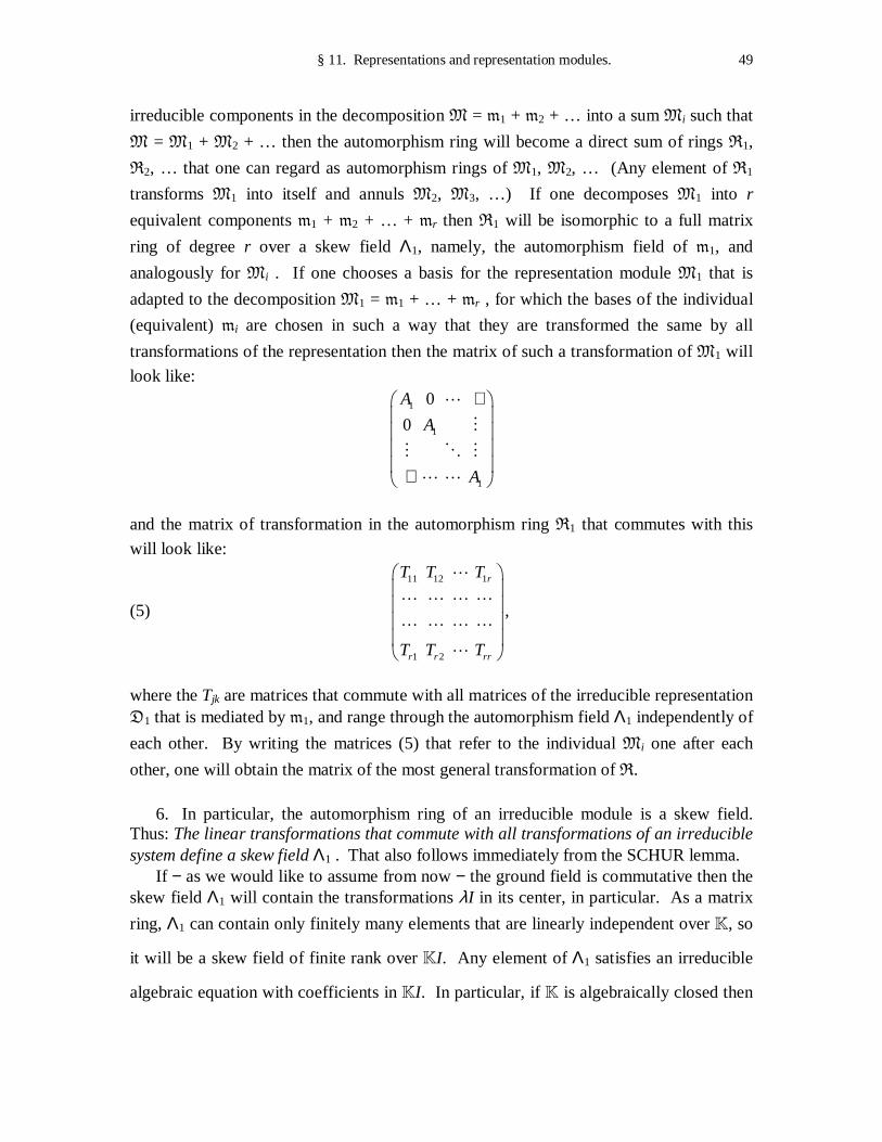
§ 11. Representations and representation modules. 49
irreducible components in the decomposition M = m1 + m2 + … into a sum Mi such that
M = M1 + M2 + … then the automorphism ring will become a direct sum of rings R1,
R2, … that one can regard as automorphism rings of M1, M2, … (Any element of R1
transforms M1 into itself and annuls M2, M3, …) If one decomposes M1 into r
equivalent components m1 + m2 + … + mr then R1 will be isomorphic to a full matrix
ring of degree r over a skew field Λ1, namely, the automorphism field of m1, and
analogously for Mi . If one chooses a basis for the representation module M1 that is
adapted to the decomposition M1 = m1 + … + mr , for which the bases of the individual
(equivalent) mi are chosen in such a way that they are transformed the same by all
transformations of the representation then the matrix of such a transformation of M1 will
look like:
1
1
1
0
0
A
A
A
⋅ ⋅
⋯
⋮
⋮ ⋱ ⋮
⋯ ⋯
and the matrix of transformation in the automorphism ring R1 that commutes with this
will look like:
(5)
11 12 1
1 2
r
r r rr
T T T
T T T
⋯
⋯ ⋯ ⋯ ⋯
⋯ ⋯ ⋯ ⋯
⋯
,
where the Tjk are matrices that commute with all matrices of the irreducible representation D1 that is mediated by m1, and range through the automorphism field Λ1 independently of
each other. By writing the matrices (5) that refer to the individual Mi one after each
other, one will obtain the matrix of the most general transformation of R.
6. In particular, the automorphism ring of an irreducible module is a skew field. Thus: The linear transformations that commute with all transformations of an irreducible system define a skew field Λ1 . That also follows immediately from the SCHUR lemma. If − as we would like to assume from now − the ground field is commutative then the skew field Λ1 will contain the transformations λI in its center, in particular. As a matrix
ring, Λ1 can contain only finitely many elements that are linearly independent over K, so
it will be a skew field of finite rank over KI. Any element of Λ1 satisfies an irreducible
algebraic equation with coefficients in KI. In particular, if K is algebraically closed then
50 II. Representations of rings and groups.
one must have Λ1 = KI, i.e.: the operator automorphisms of an irreducible representation
module with an algebraically closed coefficient field K are scalar multiples λI of the
identity I (147). The same thing is true for arbitrary ground fields when the representation is absolutely irreducible – i.e., it remains irreducible under an arbitrary algebraic
extension of the ground field K.
7. H. FITTING (148) stated a further theorem: If the representation module M is
completely reducible then there will be a one-to-one correspondence between the invariant subspaces N of M and the right-ideals r of the automorphism ring A, in which,
in particular, every decomposition of M into irreducible subspaces will correspond to a
decomposition of A into minimal right-ideals (and conversely). For a given r, one will
have N = r M, and for a given N, r will consist of those homomorphisms that map M
into N.
§ 12. Representations of hypercomplex systems. Semi-groups
of linear transformations.
A hypercomplex system – or an algebra – of rank h over K is a ring that is also an h-
dimensional vector space relative to the commutative field K. Thus, a hypercomplex
system is given by a basis (u1, …, un), and a multiplication table:
uj uk = ll jku γ∑ .
Any hypercomplex system S possesses an immediately-associated representation,
namely, the regular representation, which one obtains when one regards the system S
itself as the representation module (with S as the left operator domain and K as the right
one). The representative matrix of a quantity j ju ξ∑ in the regular representation is
obviously ljk jγ ξ∑ (l is the row index, k is the column index). The invariant subspaces
of the representation module are the left ideals, which contain all multiples r⋅⋅⋅⋅ a (r in S)
and aλ (λ in K), along with every element a. The irreducible subspaces are the minimal
left ideals. We will also call two operator-isomorphic left ideals that mediate equivalent representations equivalent. If the system S has a unity – which we will always assume in what follows – then the
regular representation will always be faithful. The types of hypercomplex systems that will be most important for us are:
§ 12. Representations of hypercomplex systems. 51
1. The division algebras (i.e., fields), in which any non-zero element possesses an inverse, and therefore unrestricted division will be possible. 2. The simple systems or full matrix rings of degree n over a division algebra Λ, which consist of all matrices with elements in Λ. 3. The semi-simple systems (or systems without radical), which decompose completely into minimal left ideals. Any semi-simple system is the direct sum of full matrix rings S1 + S2 + … + Sm, which are mutually annihilating (150):
(1) S = ν
ν∑S = ( )
,ik
i k
c νν
νΛ∑∑ ; Λν is a division algebra.
If nν is the degree of the matrix ring Sν then Sν will decompose into nν equivalent
minimal left ideals, while the left ideals of different S’s will be inequivalent. If rν is the
rank of Λν then, from (1), the rank of S will be equal to:
h = 2n rν ν∑ .
A decomposition of a semi-simple system S into left ideals:
R = l1 + l2 + … + ls
is also associated with a decomposition of the unity into idempotents: 1 = e1 + e2 + … + es , 2
ie = ei ; ei ek = 0 for i ≠ k.
An arbitrary hypercomplex system S possesses a radical – i.e., a maximal, nilpotent,
left ideal c:
cρ = 0.
c is a two-sided ideal in S, and the residue class ring S / c is semi-simple (150).
The theory of representations of hypercomplex systems will now be governed by the following theorems: Lemma. Any representation of a semi-group with unity decomposes into two components (one of which can be missing): In one of them, the unity will be represented
(150) The theorems presented go back to J. H. MACLAGAN-WEDDERBURN: Proc. London Math. Soc. 6 (1907), 77-118. For simple proofs, see B. L. VAN DER WAERDEN: Moderne Algebra II, chap. 16, or H. FITTING: Math. Ann. 107 (1932), 514-542. Cf., also the booklet on algebra by M. DUERING in this series (4 Heft 1).
52 II. Representations of rings and groups.
by the identity matrix, while the other one will consist of nothing but zeroes (i.e., the zero representation). Proof. From the lemma, one can restrict oneself to the case in which the unity of S
induces the identity transformation in the representation module M. Now, let:
S = l1 + l2 + … + ls ,
M = (u1, …, um) = ku∑S = ,
i ki k
u∑l ,
where the sum that is suggested by S does not need to be direct. Each of the modules li
uk is an operator-homomorphic image of li under the association x → x uk, so it is either
the zero module or it is operator-homomorphic to li , and therefore minimal. Therefore,
each of them either has only zero in common with the sum of the foregoing, or it is contained entirely within it. If one now drops those summands li uk in the sum that are
already contained in the sum of the foregoing then the sum will be direct. If one actually presents the left ideal lν = ( ) ( )
11 21c cν νν νΛ + Λ + … + ( )
1nc ννΛ in terms of
the irreducible representation Dν then that will imply the following additional theorems
and corollaries (151): The representation Dν of the element a = ( ) ( )
,jk jk
j k
c ν ν
να∑∑ of S [cf., (1)] will be
obtained when one defines the matrix Aν = (αik(ν)) and replaces every element αik
(ν) of the division algebra Λν with its representative matrix in the regular representation of Λν . In
the case Λν = K, the Aν already define the representation Dν , in their own right. The
irreducible representation Dν then represents the sub-ring Sν [cf., (1)] faithfully, and
represents the rings Sµ (µ ≠ν) by zero. It is of degree nν rν, so it appears in the regular
representation nν times, and because it represents Sν faithfully, it will contain 2n rν ν
linearly-independent matrices. The field Λν is inversely isomorphic to the field of the matrices that commute with the representation Dν .
Second representation theorem. The radical c will be represented by zero for an
irreducible − and therefore also for a completely-reducible − representation of an arbitrary hypercomplex system S; i.e., the representation can be regarded as the
representation of a semi-simple system. Proof. Let M be an irreducible representation module. Now, if one had cM ≠ 0 then
one would have cM = M, so:
(151) One finds that the arguments are detailed completely in the already-cited Moderne Algebra II, § 121 and § 118.
§ 12. Representations of hypercomplex systems. 53
M = cM = c2 M = … = cρ M = (0),
which is not true. Corollaries. A completely reducible representation D contains 2n rν ν∑ linearly-
independent matrices, where the summation is extended over the irreducible representations Dν of S / c that enter into D as components at least once. The
representation D then represents S / c faithfully if and only if all Dν enter into it at least
once. It follows from both representation theorems that: A faithful representation of a hypercomplex system S is completely reducible if and only if the system S is semi-
simple. It follows further from this that: A semi-group g of linear transformations is
completely reducible if and only if the hypercomplex system that consists of all linear combinations of transformations µ µλ∑A of g (viz., the “linear hull” of g) is semi-
simple. One obtains a homomorphic image g′ from an arbitrary reducible semi-group g of
linear transformations when one replaces all matrix elements in the matrices of g outside
of the irreducible diagonal boxes with zeroes. When one then necessarily goes to the linear hulls, one can then assume that g is a hypercomplex system. If g is completely
reducible then g will obviously be mapped to g′ 1-isomorphically; by contrast, if g is not
completely reducible then g will have a radical, which goes to zero under the map to g′, from the second representation theorem. It follows from this that: The semi-group g is
not completely reducible if and only if the non-zero linear combinations of the matrices of g consist of only ones that have nothing but zeroes in all of their irreducible diagonal
boxes. These linear combinations will define the radical of the linear hull of g.
The number of linearly-independent matrices in the semi-group g is therefore equal to
the sum of the numbers of linearly-independent matrices of its essentially different irreducible components in the completely reducible case, but larger than it in the other case (152). A representation Dν is called absolutely irreducible when it remains irreducible under
an extension of the ground field P to an algebraically closed field Ω. From the first
representation theorem (when applied to the ground field Ω), the number of linearly-independent matrices in this case is equal to the square of the degree of the representation (BURNSIDE’s theorem). It then follows from this that:
(rν nν)2 = 2r nν ν or rν = 1.
(152) G. FROBENIUS and I. SCHUR: S.-B. preuss. Akad. Wiss. (1906), 209-217.
54 II. Representations of rings and groups.
The same thing also follows from the fact that, from § 11, 6, the matrices that commute with the representation are scalar multiples of the identity matrix. The argument can be easily inverted, and one finds that: A representation Dν is absolutely irreducible if and only if either the number of its
linearly-independent matrices is equal to the square of its degree, or if Λν = P, or if all of
the matrices that commute with the representation are scalar multiples λI of the identity matrix I. One understands a general element of a hypercomplex system to mean a linear combination of the basis elements with undetermined coefficients. The arbitrariness in the choice of basis is expressed by the fact that an arbitrary linear substitution of the indeterminates is permissible. The system matrix of a representation is the representative matrix of the general element. For the calculation of the system matrix, we assume that the coefficient domain is algebraically closed, and that the system is semi-simple (the other cases can be brought back to this case quite easily), and we employ the basis (cjk
(ν))
that is given by (1). The general element is then ( )( )
jk jkc
νν ξ∑ , where ξ jk(ν) are
undetermined. If ∆ν is the determinant | ξ jk(ν) | then the system determinant of an
arbitrary representation that contains the irreducible represent Dν – say – sν times will be
equal to: (2) ∆ = sν
νν
∆∏ .
In particular, in the case of a regular system determinant (viz., the regular representation), one will have sν = nν . The ∆ν are obviously different, irreducible forms in the indeterminates ξ jk
(ν), and that will still be true after a linear substitution of the indeterminates. For FROBENIUS (138), the factor decomposition (2) of the system determinant defined the starting point for the theory of representations. The theorem of RABINOWITSCH (153) follows from the theorems of this and the previous paragraphs: If S is the semi-simple system with unity (or the linear hull of a completely reducible
semi-group with unity) of linear transformations of a vector space M into itself, and T is
(153) This theorem was made known to me some years ago by verbal communication. Cf., also the somewhat more specialized theorems on commuting sub-rings of simple system of R. BRAUER: J. reine angew. Math. 166 (1932), 245; K. SHODA: Math. Ann. 107 (1932), 252-258, and E. NOETHER: Math. Z.
37 (1933), 514-541. BRAUER and SHODA assumed that the center of K was complete, while BRAUER
and NOETHER assumed that S was simple. These assumptions are unnecessary, since one can reduce the
semi-simple case to the simple case (which was treated by NOETHER) by a decomposition of S into
simple systems: S = Σ Sν , which involve the decompositions M = Σ Mν and T = Σ Tν (Mν = Sν M; Tν
= automorphism ring of Mν), in which the Tν are again simple systems, from § 1.
§ 13. Representations of finite groups. 55
the system of the linear transformations that commute with all transformations of S then,
conversely, S will be the system of linear transformations that commute with all
transformations of T.
§ 13. Representations of finite groups.
The general theorems that were proved in the foregoing on semi-groups of linear substitutions are naturally true for the representation of groups, in particular. For finite groups, one has the following theorem of MASCHKE:
Any representation of a finite group g in a field P whose characteristic does not
divide the order h of the group is completely reducible. We already mentioned in § 8 how one can carry out the proof in the case of the field of complex numbers by constructing an invariant, positive, HERMITIAN form. For arbitrary fields, one employs a proof of I. SCHUR that reads (when briefly summarized): On the basis of the lemmas of § 12, one can first assume that the group identity is represented by the identity matrix, and therefore, the inverse group elements s and s−1 are also represented by inverse matrices. Now, if:
A(s) = ( ) 0
( ) ( )
P s
Q s R s
are the matrices of a reducible representation then one will define the matrix:
S = 1
in
1( ) ( )
s
R s Q sh
−∑g
.
One will then have: 0 ( ) 0
( ) ( )
I P t
S I Q t R t
= ( ) 0 0
0 ( )
P t I
R t S I
,
so the matrix system A(s) will be equivalent to a decomposable system. The problem of representing finite groups can be immediately converted, moreover, into the problem of representing hypercomplex system that was resolved already when one defines the group ring R (or R0) of the group g; i.e., the hypercomplex system
whose basis elements are the elements s1, …, sh of g. Any representation:
s → A(s)
of g can obviously be extended to a representation:
56 II. Representations of rings and groups.
Σ λi si → Σ λi A(si) of R. Conversely, any representation of R is also a representation of g, since g is
naturally contained in R. One naturally chooses the ground field of the hypercomplex
system to be the field in which g should be represented.
In particular, the regular representation of R − under which, R is its own
representation module − produces a representation of degree h of g that one likewise call
the regular representation. The matrix elements of A(s) are:
αik(s) = 1 for ,
0 otherwise,k iss s=
in this case. Since, from MASCHKE’s theorem, any representation of g is completely reducible,
the regular representation will also be completely reducible; i.e., R will decompose
completely into irreducible left ideals: R is semi-simple, where one always assumes that
the characteristic of K does not divide h. It then follows from the first representation
theorem (§ 12) that: All irreducible representation of g are already contained in the regular one and will
be generated by the left ideals of R. If the irreducible representation Dν is contained in
the regular one – perhaps n times – then its degree will be nν rν . The rank of R is:
h = 2
1
s
n rν νν =∑ ,
or
h = 2
1
s
nνν =∑ ,
resp., in the case of absolutely irreducible representations (rν = 1). One obtains another similar relation in the absolutely irreducible case from enumerating the rank of the center of R (cf., below, § 15). This rank is, on the one hand,
equal to the number s of inequivalent representations, and on the other, equal to the number of classes of conjugate group elements. Therefore, the number of inequivalent absolutely irreducible representations is equal to the number of classes of conjugate group elements.
§ 13. Representations of finite groups. 57
If one extends the ground field K in such a way that all representations decompose
into absolutely irreducible ones then the group ring R will become a direct sum of full
matrix rings S over K with matrix units cik(ν), and one will have an expression:
(1) s = ( ) ( )
,
( )ij iji j
s cν ν
να∑∑
for each group element s. From § 12, the αik
(ν)(s) will be precisely the matrix elements of the representative matrix Aν(s) of s in the representation Tν .
For the Abelian groups, the absolutely irreducible representations are of degree 2; i.e., the matrices have only one element, which, when regarded as a function of the group element a, is called a character χ(a). The characters of an Abelian group are then functions χ(a) of the group element a that have the property:
χ(ab) = χ(a) ⋅⋅⋅⋅ χ(b).
Since a finite Abelian group is a direct product of cyclic groups C1 C2 … Cr with the
generators c1, …, cr , and the orders l1, …, lr, its character can be exhibited effortlessly: One associates each cr with an arbitrary l th root of unity ζν and sets:
1 21 2( )r
rc c cρ ρ ρχ ⋯ = 1 21 2
rr
ρ ρ ρζ ζ ζ⋯ .
The product of two characters is again a character. The characters of a finite, Abelian group define an Abelian group C that is isomorphic to the given group. Any subgroup h
of the given group g will be in one-to-one correspondence with a subgroup U of the
character group, which is characterized by:
χ(a) = 1 for a in h, χ in U.
Therefore, C / U ≅ h and g / h ≅ U, because C / U is the character group of h, and U is that
of g / h.
In a precisely corresponding way, one can also characterize every normal subgroup h
of a finite group g by the fact that the elements of h will correspond to the identity matrix
for some completely-determined representation of g, or − what amounts to the same thing
in the case of field of characteristic zero − the fact that the traces of the representative matrices of the elements of h are equal to the degree of the representation (or the trace of
the identity matrix). Certain applications of the theory of representations rest upon this
58 II. Representations of rings and groups.
method, for which one is concerned with inferring the existence of normal subgroups from the properties of the group character (154). If s → A(s) and s → B(s) are two absolutely irreducible representation of a finite group g and C is an entirely arbitrary matrix then:
P = 1
in
( ) ( )t
A t C B t−∑g
will be a matrix with the property: A(s) P = P B(s).
It follows from the SCHUR lemma that P = 0 when the representations A(s) and B(s) are inequivalent; however, if they are equal then P = λI, from § 11.6. If one writes the matrix equations P = 0 (P = λI, resp.) and observes that the matrix element of C is completely arbitrary then it will follow that:
1( ) ( )ij klt
t tα β −∑ = 0 when ( ) is not equiv. to ( ),
for ( ) ( ).jk il
A s B s
A s B sω δ =
Since the left-hand side admits the permutation (ik)(jl ) for αij = βij , ωij can only be equal to ωδij . Therefore, we can also write our relation as:
(2) ( ) ( ) 1( ) ( )ij klt
t tν µα α −∑ = for = , , ,
0 otherwise.
i l j kω ν µ = =
If one sets j = k and sums over k then if h is the order of the group and nv is the degree of the representation then that will yield:
h ⋅⋅⋅⋅ 1 = nv ω.
If h is not divisible by the characteristic of the field then it can also not be nv, and we will obtain:
ω = h
nν
1.
When one multiplies (2) by αik
(ν)(s) and sums over i, what will follow is the general relation:
(3) ( ) ( ) 1( ) ( )hj klt
st tν µα α −∑ = ( ) for = , ,
0 otherwise.hl j kνωα µ ν =
(154) See, perhaps, A. SPEISER: Theorie der Gruppen von endlicher Ordnung, 2nd ed., Berlin, 1927, chap. 13.
§ 14. Restricted representations of arbitrary groups. 59
The relation (2) can then be employed to solve (1) for cik(ν). If one multiplies (1)
1
hnν
αkl(ν)(s−1) and sums over s then one will get:
(4) cik(ν) = ( ) 1( )kl
s
ns s
hνν α −∑ .
§ 14. Restricted representations of arbitrary groups.
According to J. VON NEUMANN (155), the theory of representations of finite groups that was developed in § 13 can be adapted to restricted representations of arbitrary groups G in the field of complex numbers; i.e., representations for which matrix elements dik(x)
of the representative matrix D(x) of the group element x are uniformly restricted complex-valued functions of x. In place of the group ring that was employed in § 13, one generally finds the ring of almost-periodic functions on G. A complex-valued function f(x) that is defined for all x
in G is called almost-periodic (a. p.) on G when one can select a uniformly-convergent
subsequence from any sequence of functions f(aν x bν) (156).
A mean value of an a. p. function f(x) will be defined as a constant A that (when regarded as a constant function on G) can be uniformly approximated by functions of the
form: c1 f(a1 x b1) + c2 f(a2 x, b2) + … + cn f(an x bn),
with c1 + … + cn = 1. One proves that there is one and only one mean value that is a function of f(x) (155). We denote it by Mf, or Mxf(x), when the variable x should be interpreted in relation to the one whose mean value is being defined. The matrix elements dik(x) of a restricted representation are a. p. functions of x, so the dik(aν xbν) are linear combinations of the finitely-many functions djl(x) with restricted coefficients:
dik(aν xbν) = ( ) ( ) ( )ij jl lkj l
d a d x d bν ν∑∑ .
With the help of the definition of mean value that was described above, one proves precisely, as in § 8, that every restricted representation of G leaves a positive
HERMITIAN form invariant, and is thus equivalent to a unitary one. From this, or the direct proof of SCHUR (§ 13), it then follows further that every reducible, restricted representation is completely reducible. Ultimately, as is § 13, one proves the relations:
(155) J. VON NEUMANN: Trans. Amer. Math. Soc. 36 (1934), 445-492. (156) According to BOCHNER: Math. Ann. 96 (1927), 119-147, this definition is equivalent to BOHR’s original definition in the case where G is the additive group of real numbers and f(x) is a continuous function. On that, see BOHR: Ergeb. Math. I, 5 (1932).
60 II. Representations of rings and groups.
(1) 1
1
1( ) ( ) ( ),
( ) ( ) 0, for inequivalent to ,
y ij kl jk il
y ij kl
M d xy d y d xn
M d xy d y
δ−
−
= ′ ′= D D
in which dij(x) means the matrix element of an irreducible representation D of degree n,
and kld′ means that of another irreducible representation D′. The product f × g of two a. p. functions will be defined by:
f × g(x) = My(f(x y−1) g(y)) = My(f(y) g(y−1 x).
It defines an analogy with the product of two elements 1
( )f y yh
⋅∑ and 1
( )g z zh
⋅∑ of
the group rings Rg in § 13, which will, in fact, be defined by:
1 1
( ) ( )f y y g z zh h ⋅ ⋅ ∑ ∑ =
1 1( ) ( )
x yz x
f y g z xh h =
∑ ∑
= 11 1( ) ( )
x y
f y g y x xh h
−
∑ ∑ .
The product is associative and distributive over ordinary addition f(x) + g(x), so the a. p. functions define a ring under this multiplication and addition that we will denote by RG .
With the help of the product sign, one can also write (1) as:
(2)
1( ) ( ),
( ) 0.
ij kl jk il
ij kl
d d x d xn
d d x
δ × = ′× =
These relations state that the functions: (3) cij(x) = n dij(x) fulfill the equations exactly that are characteristic of the matrix units of a full matrix ring
over the field K (cf., § 12). Therefore, any irreducible representation Dν belongs to a full
matrix ring Sν in RG , whereby the same matrix ring belongs to equivalent D, and
therefore, from (2), two different Sν will mutually annihilate each other.
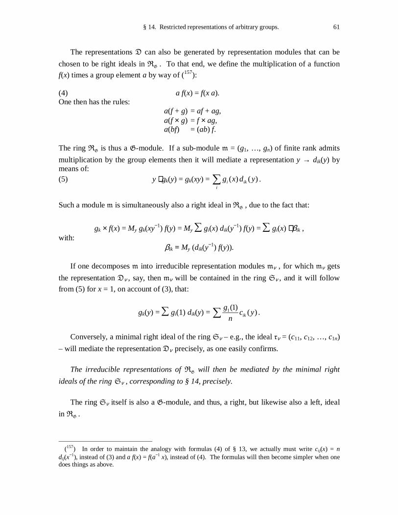
§ 14. Restricted representations of arbitrary groups. 61
The representations D can also be generated by representation modules that can be
chosen to be right ideals in RG . To that end, we define the multiplication of a function
f(x) times a group element a by way of (157): (4) a f(x) = f(x a). One then has the rules: a(f + g) = af + ag, a(f × g) = f × ag, a(bf) = (ab) f. The ring RG is thus a G-module. If a sub-module m = (g1, …, gn) of finite rank admits
multiplication by the group elements then it will mediate a representation y → dik(y) by means of: (5) y ⋅⋅⋅⋅ gk(y) = gk(xy) = ( ) ( )i ik
i
g x d y∑ .
Such a module m is simultaneously also a right ideal in RG , due to the fact that:
gk × f(x) = My gk(xy−1) f(y) = My ∑ gi(x) dik(y−1) f(y) = ∑ gi(x) ⋅⋅⋅⋅ βik ,
with: βik = My (dik(y
−1) f(y)). If one decomposes m into irreducible representation modules mν , for which mν gets
the representation Dν , say, then mν will be contained in the ring Sν , and it will follow
from (5) for x = 1, on account of (3), that:
gk(y) = ∑ gi(1) dik(y) = 1(1)( )ik
gc y
n∑ .
Conversely, a minimal right ideal of the ring Sν – e.g., the ideal rν = (c11, c12, …, c1n)
– will mediate the representation Dν precisely, as one easily confirms.
The irreducible representations of RG will then be mediated by the minimal right
ideals of the ring Sν , corresponding to § 14, precisely.
The ring Sν itself is also a G-module, and thus, a right, but likewise also a left, ideal
in RG .
(157) In order to maintain the analogy with formulas (4) of § 13, we actually must write cij(x) = n dij(x
−1), instead of (3) and a f(x) = f(a−1 x), instead of (4). The formulas will then become simpler when one does things as above.
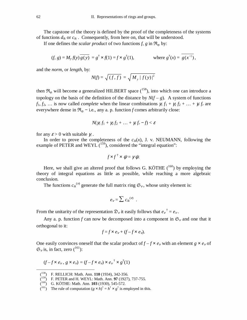
62 II. Representations of rings and groups.
The capstone of the theory is defined by the proof of the completeness of the systems of functions dik or cik . Consequently, from here on, that will be understood. If one defines the scalar product of two functions f, g in RG by:
(f, g) = My f(y) ( )g y = g† × f(1) = f × g†(1), where g†(x) = 1( )g x− , and the norm, or length, by:
N(f) = ( , )f f = 2| ( ) |yM f y
then RG will become a generalized HILBERT space (158), into which one can introduce a
topology on the basis of the definition of the distance by N(f – g). A system of functions f1, f2, … is now called complete when the linear combinations γ1 f1 + γ2 f2 + … + γr fr are everywhere dense in RG − i.e., any a. p. function f comes arbitrarily close:
N(γ1 f1 + γ2 f2 + … + γr fr − f) < ε
for any ε > 0 with suitable γi . In order to prove the completeness of the cik(x), J. v. NEUMANN, following the example of PETER and WEYL (159), considered the “integral equation”:
f × f † × ψ = γ ψ. Here, we shall give an altered proof that follows G. KÖTHE (160) by employing the theory of integral equations as little as possible, while reaching a more algebraic conclusion. The functions cik
(ν) generate the full matrix ring Sν , whose unity element is:
eν = ∑ cik(ν) .
From the unitarity of the representation Dν it easily follows that eν
† = eν .
Any a. p. function f can now be decomposed into a component in Sν and one that it
orthogonal to it: f = f × eν + (f – f × eν).
One easily convinces oneself that the scalar product of f – f × eν with an element g × eν of Sν is, in fact, zero (161):
(f – f × eν , g × eν) = (f – f × eν) × eν
† × g†(1)
(158) F. RELLICH: Math. Ann. 110 (1934), 342-356. (159) F. PETER and H. WEYL: Math. Ann. 97 (1927), 737-755. (160) G. KÖTHE: Math. Ann. 103 (1930), 545-572. (161) The rule of computation (g × h)† = h† × g† is employed in this.
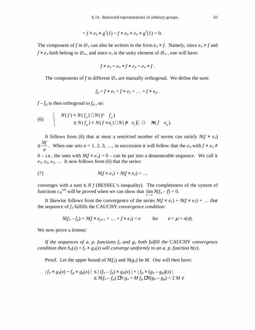
§ 14. Restricted representations of arbitrary groups. 63
= f × eν × g†(1) − f × eν × eν × g†(1) = 0. The component of f in Sν can also be written in the form eν × f. Namely, since eν × f and
f × eν both belong to Sν , and since eν is the unity element of Sν , one will have:
f × eν = eν × f × eν = eν × f .
The components of f in different Sν are mutually orthogonal. We define the sum:
fµ = f × e1 + f × e2 + … + f × eµ .
f – fµ is then orthogonal to fµ , so:
(6) 1 2
( ) ( ) ( )
( ) ( ) ( ) ( ).
N f N f N f f
N f N f e N f e N f eµ µ
µ µ
= + − ≥ = × + × + + × ⋯
It follows from (6) that at most a restricted number of norms can satisfy N(f × eν)
≥ Nf
n. When one sets n = 1, 2, 3, …, in succession it will follow that the eν with f × eν ≠
0 – i.e., the ones with N(f × eν) > 0 – can be put into a denumerable sequence. We call it e1, e2, e3, … It now follows from (6) that the series: (7) N(f × e1) + N(f × e2) + … converges with a sum ≤ N f (BESSEL’s inequality). The completeness of the system of functions cik
(ν) will be proved when we can show that limν →∞
N(fν – f) = 0.
It likewise follows from the convergence of the series N(f × e1) + N(f × e2) + … that the sequence of fν fulfills the CAUCHY convergence condition:
N(fν – fµ) = N(f × eµ+1 + … + f × eν) < e for ν > µ > n(ε). We now prove a lemma: If the sequences of a. p. functions fν and gν both fulfill the CAUCHY convergence condition then hν(x) = fν × gν(x) will converge uniformly to an a. p. function h(x). Proof. Let the upper bound of N(fν) and N(gν) be M. One will then have: | fν × gν(x) − fµ × gµ(x) | ≤ | (fν – fµ) × gν(x) | + | fµ × (gν – gµ)(x) | ≤ N(fν – fµ) ⋅⋅⋅⋅ N gν + M fµ ⋅⋅⋅⋅ N(gν – gµ) < 2 M ε
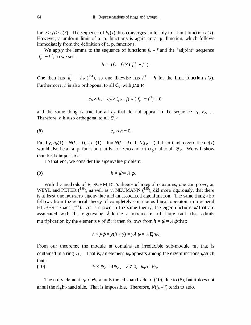
64 II. Representations of rings and groups.
for ν > µ > n(ε). The sequence of hν(x) thus converges uniformly to a limit function h(x). However, a uniform limit of a. p. functions is again an a. p. function, which follows immediately from the definition of a. p. functions. We apply the lemma to the sequence of functions fν – f and the “adjoint” sequence
†fν − f †, so we set:
hν = (fν – f) × ( †fν − f †).
One then has †hν = hν (161), so one likewise has h† = h for the limit function h(x).
Furthermore, h is also orthogonal to all Sµ with µ ≤ ν:
eµ × hν = eµ × (fν – f) × ( †fν − f †) = 0,
and the same thing is true for all eµ that do not appear in the sequence e1, e2, … Therefore, h is also orthogonal to all Sµ :
(8) eµ × h = 0. Finally, hν(1) = N(fν – f), so h(1) = lim N(fν – f). If N(fν – f) did not tend to zero then h(x) would also be an a. p. function that is non-zero and orthogonal to all Sν . We will show
that this is impossible. To that end, we consider the eigenvalue problem: (9) h × ψ = λ ψ. With the methods of E. SCHMIDT’s theory of integral equations, one can prove, as WEYL and PETER (159), as well as v. NEUMANN (155), did more rigorously, that there is at least one non-zero eigenvalue and an associated eigenfunction. The same thing also follows from the general theory of completely continuous linear operators in a general HILBERT space (158). As is shown in the same theory, the eigenfunctions ψ that are associated with the eigenvalue λ define a module m of finite rank that admits
multiplication by the elements y of G; it then follows from h × ψ = λ ψ that:
h × yψ = y(h × y) = yλ ψ = λ ⋅⋅⋅⋅ yψ.
From our theorems, the module m contains an irreducible sub-module mν that is
contained in a ring Sν . That is, an element ψν appears among the eigenfunctions ψ such
that: (10) h × ψν = λψν ; λ ≠ 0, ψν in Sν .
The unity element eν of Sν annuls the left-hand side of (10), due to (8), but it does not
annul the right-hand side. That is impossible. Therefore, N(fν – f) tends to zero.
§ 14. Restricted representations of arbitrary groups. 65
Using completeness, v. NEUMANN (155) has proved that a. p. functions can be uniformly approximated by linear combinations of the dik(x) with a method of N. WIENER. All of the theorems and proofs above remain true verbatim when one restricts oneself to a topological group (162) with continuous a. p. functions and a continuous representation. There are topological groups for which all restricted representations, and thus also all a. p. functions, are continuous (163), namely, the semi-simple, continuous groups, whose representation theory has been developed by CARTAN and WEYL (164). There are even groups that possess no restricted representations besides the identity representation and
on which the only a. p. are therefore the constants. The real projective group PSL(n, P)
belongs to them. However, there are also groups on which all continuous functions are a. p. Clearly, that is the case for compact, topological groups. The completeness theorem is even true for all continuous function for these groups. We refer to v. NEUMANN (155) for a thorough investigation of these different possibilities. The absolutely irreducible restricted representations of Abelian groups G are given by
one-rowed matrices, and thus by complex numbers of modulus one; these are again called characters χ(a). Following PALEY and WIENER (165) or ALEXANDER (165a), one obtains them when one totally orders the generators of G and determines the value of a
character χ for each generator a in such a way that it follows from:
ah = ha νν
ν∏ ,
where the aν run through the a in the total ordering, that:
χ(a)h = ( )ha νν
νχ∏ .
Another method, which was given by A. HAAR (166) for denumerable Abelian groups and was extended to separable, compact-in-the-small, Abelian, topological groups by v. NEUMANN (155), generally does not yield all characters, but only a family of characters ϕ(a, λ) that are BAIRE functions of a real parameter λ that are also continuous functions of a in the topological case that have the property that lim ϕ(aν, λ) = 1 implies that lim aν = 1 for all λ. If G is denumerable then the χ(a, λ), as functions of λ, define a complete
orthogonal system relative to a monotone regulating function (Ger: Belegunsfunktion) (167).
(162) For this concept, see F. LEJA: Fundam. Math. 9 (1927), 37-44. – R. BAER: J. reine angew. Math. 160 (1929), 208-226. – D. VAN DANTZIG: “Studien over topologische algebra,” Diss. Groningen 1931. (163) B. L. VAN DER WAERDEN: Math. Z. 36 (1933), 780-786. (164) See footnotes 73 and 74 in I, § 8. See also footnote 159. (165) N. WIENER and R. E. A. C. PALEY: Proc. Nat. Acad. Sci. U. S. A 19 (1933), 253-257. (165a) J. F. ALEXANDER: Ann. of Math., II. s. 35 (1934), 389-395. (166) A. HAAR: Math. Z. 33 (1931), 129-159. (167) L. PONTRJAGIN: Ann. of Math., II. s. 35 (1935), 361-388.
66 II. Representations of rings and groups.
The continuous characters of an Abelian, topological group again define an Abelian, topological group Γ when products and limits in Γ are defined by:
( ) ( ) ( ),
lim , when lim ( ) for all .
a a a
a aν ν
ψ χ ψ χχ χ χ
⋅ = ⋅ =
If G is discrete and denumerable then Γ will clearly be compact; on the other hand, if G
is compact then Γ will discrete and denumerable (167). If G is compact in the small and
separable then Γ will also be so (167a). In all of these cases, the groups G and Γ define a
group pair, in the sense of L. PONTRJAGIN (167); i.e., a product χ ⋅⋅⋅⋅ a = χ(a) is defined for every a in G and χ in Γ that is a real number with absolute value one that depends
continuously upon χ and a individually and possesses the distributive properties:
χa ⋅⋅⋅⋅ χb = χ ⋅⋅⋅⋅ ab; ψ a ⋅⋅⋅⋅ χa = ψχ ⋅⋅⋅⋅ a. In addition, the group pair is orthogonal; i.e., if χa = 1 for some χ and all a then it will follow that χ = 1, and if χa = for some a and all χ then it will follow that a = 1. According to PONTRJAGIN (167), in the case where G is discrete and denumerable −
and thus compact – any subgroup H of G will be in one-to-one correspondence with a
closed subgroup Φ of Γ, such that Φ will consist of the χ with χa = 1 for all a in H, and
conversely H will consist of the a with χa = 1 for all a in Φ. One has, moreover: If G
and Γ define an orthogonal group pair and if G is denumerable and Γ is compact then Γ
will be the character group of G and G will be the group of continuous characters of Γ.
It follows from this that: If Γ is the character group of G then G will be the group of
continuous characters of Γ, and conversely. E. R. VAN KAMPEN (167a) has adapted these theorems to pairs of compact-in-the-small, separable, Abelian groups.
§ 15. Traces and characters.
1. Definition and general properties.
If a representation D of a semigroup g is given then we will consider the trace of the
representative matrix A of an element a to be a function of a and denote it by SD(a) or by
S(a). In particular, if g is a group then S(b−1a b) = S(a). The trace then depends upon
only the class of the group element a.
(167a) E. R. VAN KAMPEN: Proc. Nat. Acad. Sci. U. S. A. 20 (1934), 434-436. A further paper by the same author in which the theory of characters will be developed systematically will appear in Ann. of Math. 36 (1935).
§ 15. Traces and characters. 67
The trace of a matrix of a reducible system is the sum of the traces of the irreducible components. Thus, if the irreducible representations Dν enter into a representation of a
semigroup kν times as diagonal components then:
(1) SD(a) = ∑ kν ( )S aνD
.
If g is a hypercomplex system then the traces of the elements of the radical will
always be zero, since they will be represented by zeroes in all irreducible representations. The trace in the regular representation is called the regular trace. The trace of an element s of a finite group in the regular representation is zero for s ≠ 1 and equal to the order h of the group for s = 1, as one infers immediately from the formula for the matrix elements of the regular representation (§ 13). In fields with characteristic zero, one has the theorem: Two completely reducible representations D, D′ of a semigroup g are equivalent only
if their traces coincide (152). Without the assumption of characteristic zero, the cited theorem is not true, in general, but it is true for two irreducible representations. The traces of the absolutely irreducible representations of a semigroup are called characters, and will be denoted by χ(a) or χν(a). Since one can absolutely reduce any representation by going to an algebraically closed field, any trace will be a sum of characters (168). The trace of an individual group element is likewise the sum of characters of a cyclic group, so in the case of a finite group, it will be a sum of roots of unity.
2. The KRONECKER product representation.
If two representations of a semigroup g by linear transformations of the vector spaces
(u1, …, um) and (v1, …, vn) are given then one can regard the basis vectors ui , vj as indeterminates and define the m ⋅⋅⋅⋅ n products ui vj ; these will likewise be linearly transformed by the group g. If A = (aik) and B = (bjl) are the representative matrices of a
group element s in the two given representations then γij,kl = αik βjl (i, j are row and k, l are column indices) is the matrix by which the ui vj will be transformed; one calls it the KRONECKER product matrix A × B. The product transformations again define a representation of g: viz., the product representation. The trace of the product matrix is
equal to the product of the traces of the matrices A and B. If one denotes the irreducible representations of a semigroup by D1, D2, …, and one
assumes that the product representation Dλ × Dµ includes the irreducible component Dν
− say − cνλµ times then one can write:
(168) One also refers to an arbitrary integer linear combination of characters − and in particular, the trace of an arbitrary representation – as a composite character.
68 II. Representations of rings and groups.
Dλ × Dµ = cνλµ ν
ν∑ D .
For the characters χν of the representations Dν , it follows from this that:
(2) χλ(s) χµ(s) = ( )c sν
λµ νν
χ∑ .
3. The system discriminant and complementary bases.
A sufficient condition for the semi-simplicity of a hypercomplex system is the non-vanishing of the regular trace determinant – or regular discriminant: (3) D = | S(uµ vν) | that is defined by any two bases (u1, …, un) and (v1, …, vn) of the system, or – what amounts to the same thing – the existence of a complementary basis (w1, …, wn) to any basis (u1, …, un), which has the property:
S(uµ wν) = δµν (= 0 or 1). The fact that one always has D = 0 for a system with a radical will become clear when one chooses u1 in the radical, since all S(u1 wν) = 0 then. In the case of the group ring of a group whose order h is not divisible by the characteristic, one will always have D ≠ 0, so the elements 1h s−1 will define a complementary basis to the basis of the group element s:
(4) S(st) = 1
1
1 for ,
0 for .
h t s
t s
−
−
⋅ =
≠
The semi-simplicity of the group ring will follow from this once more. If one expresses the trace in (4) in terms of the characters then one will obtain:
∑ nν χν(st) = 1
1
1 for ,
0 for ,
h t s
t s
−
−
⋅ =
≠
or, when one introduces the matrices (αjk
(ν)) of the absolutely irreducible representations:
(5) ,j k
nνν∑∑ αjk
(ν)(s)αkj(ν)(t) =
1
1
1 for ( ),
0 for ( ).
h t s
t s
−
−
⋅ =
≠
The basis that is complementary to the basis (cjk
(ν)) is ( 1nν− cjk
(ν)), as one easily verifies.
§ 15. Traces and characters. 69
4. The relations between the characters.
When one sets h = j, k = l and sums over j and l, it will follow from equation (3), § 13 that:
(6) 1( ) ( )t
st tν µχ χ −∑ = ( ) for = ,
0 for .
sνωχ ν µν µ
≠
In particular, for s = 1, one will obtain the orthogonality relations of the character:
(7) 1( ) ( )t
t tν µχ χ −∑ = 1 ( = ),
0 ( ).
h ν µν µ
⋅ ≠
The orthogonality relations can thus be employed to make the decomposition of a given representation D into absolutely irreducible ones possible by mere trace
calculations. Namely, if: (8) D = cν ν
ν∑ D , so SD(s) = ( )c sν ν
νχ∑ ,
then it will follow from (7) that:
1( ) ( )s
s S sνχ −∑ D = h cν ⋅⋅⋅⋅ 1.
One determines the numbers cν from this (in the case of characteristic zero).
1( ) ( )s
S s S s−∑ D D = h ⋅⋅⋅⋅ 2 1cν ⋅∑ ,
so: A representation D in a field of characteristic zero is absolutely irreducible if and
only if one has: 1( ) ( )
s
S s S s−∑ D D = h ⋅⋅⋅⋅ 1
for its trace. The trace relation (8) often finds applications in the theory of invariants when one must determine the number of linearly-independent vectors that remain invariant under a representation D of a group g. Namely, this number is obviously equal to the coefficient
c1 of the identity representation D1 in the decomposition (8).
We now assume that the ground field is a number field. The characters χ, as sums of roots of unity, are algebraic numbers then, and indeed χ(s−1) is complex conjugate to χ(s). It now follows from (6) (with µ = ν) in a known way that ω, as the root of the secular equation:
70 II. Representations of rings and groups.
| χ(st−1) – δst ω | = 0, is likewise a whole algebraic number; it then follows that: The degree of an absolutely reducible representation is a divisor of the order of the group.
8. The center of the group ring.
The center of a semi-simple hypercomplex system S over an algebraically closed
field consists of the elements z that commute with all elements of S, so they will be
represented by a multiple of the identity matrix in any absolutely irreducible representation. The formula:
r = ( ) ( )
,
( )jk jkj k
r cν ν
να∑∑ ,
which is true for any element r of S, will then reduce to:
(9) z = ( )( ) kk
k
z c νν
να∑ ∑ = ( )z Iν ν
να∑ ,
for r = z. The Iν = ( )
kkk
c ν∑ are idempotent elements of the center, namely, the unity elements
of the full matrix rings Sν into which S decomposes. The αν(z) are the irreducible
representations (of degree 1) of the center. Obviously, the relation: (10) χν(z) = nν αν(z) exists between the characters χν(z) = ( )
kkk
να∑ and the αν(z).
In the case of the group ring, z = ssλ∑ belongs to the center if and only if tzt−1 = z
for any group element t, and that comes down to saying that all of the elements tst−1 that are conjugate to an s have the same coefficients λs . If one then sets ks equal to the sum of all different elements tst−1 of the class of s then the ks will generate the center, and relation (9) will become:
(11) ks = ∑ αν(ks) Iν = ( )sk
In
νν
ν
χ∑ = ( )sh
s In ν ν
ν ν
χ∑ ,
in which hs is the number of elements in the class of s. The solution of this formula for Iν is obtained from (4), § 13, when one sets l = k in it and sums over k:
(12) Iν = 1( )s
ns s
hν
νχ −∑ = 1( ) ss
n' s k
hν
νχ −∑ .
§ 16. The decomposition of irreducible representations by extension of the ground field. 71
In the last summation ∑′, s runs through a system of representatives for all classes of the group. A comparison of (11) with (12) yields that the matrices (χν(s)) and
1( )shs
h νχ −
, in which the row (column, resp.) index s runs through a system of
representatives of all classes, are inverse to each other. The orthogonality relations (11) say the same thing. One can also express this by the formula:
(13) ( ) ( )s tν νν
χ χ∑ = 1
1
0 for ,
/ for .s
t s
h h t s
−
−
≠ =
The product ks kt of two generators of the center is again an element of the center, and thus, a (integer) linear combination of the generators kr :
ks kt = rst rg k∑ .
The fact that the functions αν(z) define a representation of the center is expressed by the formula:
αν(ks) αν(ks) = ( )rst rg kνα∑ ,
which is converted into: (14) hs htχν(s) χν(t) = ( )r
st rn g h rν νχ∑
(i.e., summation over a system of representatives of the classes) after multiplying by nν
2, due to (10). G. FROBENIUS (169) first defined the character χ(s) by formula (14). A. HAAR (170) gave another basis for the theory of characters that is independent of the theory of representations, and which is also valid for certain infinite groups. Most of the formulas in this paragraph were derived only under the assumption that the order h of the group was not divisible by the characteristic of the field, and thus that the group ring was semi-simple. However, that is not true for formulas (2), (6), (7), (8), (10), (14), which have general validity.
§ 16. The decomposition of irreducible representations by extension of the ground field.
The question of how an irreducible semigroup of linear transformations can
decompose under an extension of the ground field P to a commutative field K reverts
immediately to the question of the behavior of a simple hypercomplex system S under an
extension of the ground field. Namely, if S is the linear hull of the given semigroup G
(169) G. FROBENIUS: S.-B. preuss. Akad. Wiss. (1896), 985-1021. (170) A. HAAR: Acta Litt. Sci. Szeged 5 (1932), 172-186.
72 II. Representations of rings and groups.
then S will be a simple hypercomplex system over P, and the given representation of S
by linear transformations will be mediated by a left ideal l of S. Under an extension of P
to K, S will go to a hypercomplex system SK, and l will go to a left ideal l
K of S; one
then simply treats the problem of how this left ideal in SK will decompose into
irreducible left ideals. Since this question was discussed thoroughly in the book on algebra (volume IV, book 1) in these “Ergebnisse,” here, it will suffice to summarize briefly the most important results without proof (171). Let S be a full matrix ring of
degree n over a division algebra Λ, let Z be the center of Λ, and let D be the given
representation of S as an irreducible semigroup of linear substitutions.
1. If Z or K or both of them are separable over P then the system SK will be semi-
simple, so any representation of S in K will be completely reducible. In particular: Any
irreducible or completely reducible representation will remain completely reducible under a separable extension of the ground field.
In the sequel, we will assume that Z is separable over P.
2. The ideal lK decomposes into just as many irreducible left ideals as the ring Λ
K,
only of n times greater rank. The ring ΛK decomposes into just as many simple systems
(two-sided ideals of the ring) as its center ZK .
Any of these simple systems can be further decomposed into only equivalent left ideals; however, the left ideals of different systems are inequivalent. For the representation D, this says that it decomposes into just as many inequivalent components
as ZK ; each of these components can then be further decomposed into equivalent
irreducible representations.
3. If K is Galoisian, in particular, then the different simple subsystems of ΛK, and
therefore also the inequivalent components of the representation D, will be conjugate
relative to P; i.e., they will go to each other under the automorphisms of K.
(171) The theorems of these paragraphs (to the extent that they relate directly to the semigroup G) go back to I. SCHUR: S.-B. preuss. Akad. Wiss. (1906), 64-184; Trans. Amer. Math. Soc. 10 (1909), 159-175; their hypercomplex basis and refinement goes back to E. NOETHER; Math. Z. 37 (1933), 514-541. For the historical development, see H. TABER: C. R. Acad., Paris 142 (1906), 948-951; L. E. DICKSON: Trans. Amer. Math. Soc. 4 (1903), 434-436.
§ 16. The decomposition of irreducible representations by extension of the ground field. 73
If one is interested in the absolutely irreducible representation D′ into which D
decomposes under a sufficient further (e.g., algebraically closed) extension of P, then
from 3, it will suffice to consider one of these representations D′; the remaining ones will
certainly be conjugate to it and will appear in D equally often.
A field K in which an absolutely irreducible representation D′ of D splits is called a
splitting field. A field in which D decomposes completely into absolutely irreducible
representations is called a decomposition field. The number m that gives how often the absolutely irreducible representation D′ appears in D is called the SCHUR index of D′ or
D relative to the field P.
4. Any splitting field K envelops a field Z1 that is equivalent to Z. A component D1
of the given representation D that is irreducible in Z1 splits off from D in Z1 , which
further splits into m equivalent components D′ in K.
In the event that the index m is not divisible by the characteristic of the field, the field Z1 will be generated by the characters of the absolutely irreducible representation D′. One can also obtain the representation D when one identifies Z with Z1 and regards S as
a hypercomplex system over Z and l as a representation module relative to Z. Regarding
Z = Z1 to be the ground field, instead of P, simplifies the investigation insofar as S will
then become a normal, simple system – i.e., one whose center is the ground field. The concepts of decomposition field and splitting field coincide relative to these ground fields: 5. The division algebra Λ has rank m2 relative to Z . The degree of any splitting
field K over Z is divisible by m. The splitting fields of smallest degree have degree m and
are isomorphic to the maximal, commutative sub-field of Λ. Any splitting field of degree mq is isomorphic to a maximal, commutative sub-field of the full matrix ring of degree q over Λ, and any such maximal, commutative sub-field of Λq is a splitting field. In conclusion, we mention a theorem that is easy to prove for completely reducible representations:
If two representations of a semigroup G by linear transformations in a field P are
equivalent in an extension field K then they will also be equivalent in the ground field P.
74 II. Representations of rings and groups.
Proof (172): First of all, assume that the ground field P has infinitely many elements,
or at least, more than the degree of the representation would imply. The equivalence of two representations a → A1 and a → A2 would be equivalent to the solubility of a system of linear equations TA1 = A2T and an inequality | T | ≠ 0 for the elements of the matrix T.
If such a system were soluble in the field K then it would also be already soluble in the
ground field P, assuming that P contains more elements than the degree of the inequality
would imply.
Secondly, assume P has finitely many elements. If two representations in K are
equivalent then they will also be equivalent in a finite extension field Σ of P with
sufficiently many elements. If M = u1 P + … + um P and N = v1 P + … + vm P are the
representation modules of the semigroup G then their extension modules MΣ = u1 Σ + …
+ um Σ and MΣ = v1 Σ + … + vm Σ will be operator isomorphic as (G, Σ)-modules, and
therefore all the more so as (G, P)-modules. Now, if (σ1, …, σg) is a P-basis of Σ then
MΣ can also be written in the form:
(1) MΣ = Mσ1+ …+ Mσg .
The individual summand Mσi is operator isomorphic to M by means of the association u
→ uσi . If one thinks of M and MΣ as being written in the form of direct sums of directly
indecomposable summands, according to the REMAK-SCHMIDT theorem (§ 11.4), then, on the basis of (1), MΣ will contain each summand precisely g times as often as M.
Now, if MΣ and NΣ contain directly indecomposable summands just as often then the
same thing will also be true for M and N.
§ 17. Factor systems.
Let D be an absolutely irreducible representation of a normal, simple hypercomplex
system S in a finite, separable extension field K = P(ϑ) of the ground field P. D might
go to Dα by means of the field isomorphisms Γα, which take ϑ = ϑ1 to its conjugate
quantities ϑα . Since the representations Dα are all equivalent, there will be non-singular
matrices Pαβ in the field P(ϑα , ϑβ) that transform Dβ into Dα :
(1) Dα = Pαβ Dβ
1Pαβ− .
(172) The proof goes back to E. NOETHER and was partially presented by M. DEURING: Math. Ann. 107 (1932), 144.
§ 17. Factor systems 75
One can obviously choose the Pαβ in such a way that any isomorphism of P(ϑα, ϑβ)
that takes ϑα , ϑβ to a conjugate pair ϑγ , ϑδ also takes Pαβ to Pγδ . To that end, one needs only to choose a pair (ϑα , ϑβ) arbitrarily from any class of conjugate pairs in order to determine a Pαβ and derive the remaining Pγδ from Pαβ by the isomorphisms in question. One can thus choose P11 = I. The matrix Pαβ Pβγ transforms Dγ into Dα ; one then has:
Pαβ Pβγ = cαβγ Pαγ ,
where cαβγ is a non-zero number in P(ϑα, ϑβ , ϑγ). These numbers define the factor
system of the representation D of S in the field K over P. The following conditions are
characteristic of such a factor system (173): 1. c111 = 1, 2. cαβγ cαγδ = cαβδ cβγδ , 3. S cαβγ = cα′ β′ γ′ , when S is an isomorphism that takes ϑα, ϑβ , ϑγ to ϑα′, ϑβ′ , ϑγ′ . If one replaces Pαβ with kαβ Pαβ , where the numbers kαβ must fulfill the same conjugacy conditions as the Pαβ, then the c will go to an “associated factor system”:
cαβγ′ = k k
kαβ βγ
αγ
cαβγ .
If one regards associated factor systems as not being different then the factor system cαβγ
will be determined uniquely by the hypercomplex system S and the field K(ϑ). For a
given cαβγ that fulfills the conditions 1, 2, 3, one obtains a hypercomplex system S with
just this factor system when one constructs all matrices of the form:
11( )c lκλ κλ
− (κ rows, λ columns),
where the lκλ run through all numbers in P(ϑα, ϑβ) that fulfill the same conjugacy
conditions as the kκλ do above. The totality of these matrices is absolutely irreducible and linearly closed; it then faithfully represents a simple hypercomplex system S. This
representation is equivalent to a representation that is rational in P(ϑ) and has the factor
system cαβγ (174).
The fundamental theorem in the theory of factor systems reads: (173) See R. BRAUER: Math. Z. 28 (1928), 677-698. (174) R. BRAUER: Math. Z. 30 (1929), 90.
76 II. Representations of rings and groups.
S is a full matrix ring over the ground field P if and only if the factor system is
associated with the identity system cαβγ = 1 (175). If one brings into play the easily-proved facts that the product S × T of two normal,
simple, hypercomplex systems belongs to the product of the factor systems cαβγ ⋅⋅⋅⋅ dαβγ , and the inverse isomorphism system S′ belongs to the inverse factor system 1cαβγ
− then it
will follow that S × S′ has the factor system one, so it will be a full matrix ring over P
(176). If one now divides the algebra S into classes, when one counts all full matrix rings
over the same division algebra Λ in one class, then these classes will define a group under
the multiplication S × T: viz., the BRAUER algebra class group, in which the class of P
plays the role of the identity element and the class of S′ plays the role of the inverse
element to the class of S. The algebra classes with fixed decomposition field K define a
subgroup of the algebra group that is homomorphic to its group of factor systems, and in fact is 1-isomorphic to it on the basis of the main theorem above. It follows from this
that any algebra class with a given center P and decomposition field K will be
determined uniquely by its factor system cαβγ ; in particular, a division algebra with a
given P and K will then be determined uniquely by its factor system.
Naturally, an extension field K′ of K is also a decomposition field of S with K; the
associated factor system is determined from that of K in a closely-related way: one will
have cαβγ′ = cαβγ , when the isomorphisms Γα′ , Γβ′ , Γγ′ of K′ yield the isomorphisms Γα ,
Γβ , Γγ when they are applied to K.
If one chooses K′ to be a Galois field Ω over P, in particular, and employs the
elements S, T, U, … of the Galois group as indices, instead of the numbers α′, β′, γ′, then one can also construct a hypercomplex system S that belongs to the given factor system
in the following way: S envelops Ω, and each automorphism S of K belongs to a basis
element uS of S relative to Ω, such that one will have:
S = S
S
uΩ∑ = SS
u Ω∑ .
For each ω in Ω, one will have: ω uS = uS (S ω),
(175) A. SPEISER: Math. Z. 5 (1919), 1-6; cf., also I. SCHUR: Math. Z. 5 (1919), 7-10 and R. BRAUER: S.-B. preuss. Akad. Wiss. (1926), 410-416. (176) A direct proof of this theorem is given by E. NOETHER: Math. Z. 37 (1933), 532.
§ 18. Integrality properties. Modular representations. 77
uS uT = uST 1
, ,1ST Sc− .
S is called the folded product of the field Ω with its GALOIS group.
For more on the theory of factor systems and the folded product, we refer to the cited literature, in particular, to the book on algebra by M. DUERING in this collection (Band IV, Heft 1).
§ 18. Integrality properties. Modular representations.
W. BURNSIDE has proved (177): A semigroup of linear substitutions whose matrix elements are rational numbers with reduced denominators is equivalent to an integer subgroup. The proof of this, which is presented by SPEISER (178), yields the following generalization of this theorem: If the matrix elements of the semigroup g are numbers in a finite algebraic number
field with reduced denominators then g will be equivalent to a semigroup with integer
algebraic matrix elements in a suitable extension field. In particular, the theorems that were mentioned for a representation of a finite group (more generally, for a representation of an “ordering” of a hypercomplex system, as well) will be true in an algebraic number field. Two integer representations A(s), B(s) of a semigroup are called integer equivalent when they can be taken to each other by transformations with a unimodular, integer matrix, or – what amounts to the same thing – when their integer representation modules are operator isomorphic. Rational equivalence is necessary, but not sufficient, for integer equivalence. According to C. JORDAN, however, the integer representations of a semigroup that are rationally equivalent to a given rationally irreducible representation decompose into only finitely many classes of mutually integer equivalent representations (179). If one extends the given representation to a semi-simple, hypercomplex system S
then one can choose the representation module for it and all representations that are equivalent to it to be a minimal left ideal l of S. The integer linear combinations of the
matrices of the given representation define an “ordering” o in S, and the integer
representations will be mediated by an o-module that is contained in l. When one
(177) W. BURNSIDE: Proc. London Math. Soc. (2) 7 (1909), 8-13. (178) A. SPEISER: Theorie der Gruppen von endlicher Ordnung, 2nd ed., Berlin, 1927, § 65. (179) C. JORDAN: J. École polytechn. 48 (1880), 111-150. – Another proof is in L. BIEBERBACH: Nachr. Akad. Wiss. Göttingen (1912), 207-216. – L. BIEBERBACH and I. SCHUR: S.-B. preuss. Akad. Wiss. (1928), 523-527.
78 II. Representations of rings and groups.
multiplies these o-modules with suitable natural numbers, one can convert them into
ideals of the ring o. JORDAN’s theorem then means the same thing as another one that
says that there are only finitely many classes of mutually isomorphic ideals in o that are
contained in the given l of S. This finitude of the ideal classes can also be proved with
the classical ideal-theoretic methods (180). One understands the term modular representations of a group to mean the representations in a field of characteristic p, or especially a Galois field GF(pf ). We shall now examine the relations that exist between modular and non-modular representations. Let D1, …, Dr be a complete system of inequivalent absolutely irreducible
representations of a finite group g that may be assumed to be integer algebraic for a
suitable algebraic number field K. If one now reduces these representations modulo a
prime ideal p of K then one will obtain just as many modular representations of g in
GF(pf). If the characteristic p of GF does not go into the order h of the group then the representations Dν will also remain irreducible and inequivalent modulo p, and they will
exhaust all absolutely irreducible representations of g in fields of characteristic p.
Proof. From § 13, formula (4), only integer algebraic numbers, divided by the order h of the group, will appear as coefficients in the expressions for the matrix units cik
(ν) of the group ring as linear combinations of the group elements s. Thus, the formulas will remain meaningful modulo p. The rules of calculation cik
(ν)ckl (ν) = cil
(ν), etc., as well as
the formula s = ( ) ( )( )ik iks cν να ⋅∑ , will likewise remain true. However, these formulas
also define the decomposition of the group ring into full matrix rings relative to the ground field GF(pf ); therefore, the various absolutely irreducible representations of g by
matrices mod p will also be given in GF.
The representations of finite groups g in fields whose characteristic p goes into the
order h of the group were investigated by DICKSON (181). In the extreme case h = pg, the identity representation is the only irreducible representation; any representation can then be brought into the form (182):
21
1
1 0 0
1 0
1n
α
α
⋯
⋯
⋮ ⋱ ⋮
⋯ ⋯
.
DICKSON deduced from this: If g contains a Sylow group h of order pg then any irreducible representation of g in a
field of characteristic p will be contained in that representation that is induced by the (180) C. G. LATIMER: Bull. Amer. Math. Soc. 40 (1934), 433-435. (181) L. E. DICKSON: Trans. Amer. Math. Soc. 8 (1907), 389-398. (182) Another proof of this was given by E. SPEISER: Theorie der Gruppen von endlicher Ordnung, 2nd ed., § 69.
§ 19. Relations between the representations of a group and those of its subgroups. 79
identity representation of the Sylow group h (cf., § 19). The regular representation
contains this induced representation precisely pg times as a diagonal component, but it is not, however, completely reducible. L. E. DICKSON (183) has calculated the characters of the modular representations for some examples of finite groups with the help of formulas (6), § 15. The example of A5 ≅
SL(4, 2) shows that there are modular representation that cannot arise from integer algebraic representations by residue classes modulo p, so A5 has no integer representation
of degree 2. R. BRAUER communicated to me the fact that the number of inequivalent absolutely reducible, modular representations of characteristic p is equal to the number of those classes of conjugate elements in which the order of the element is relatively prime to p. I hope that he will publish this result soon. Finally, let us mention a theorem of MINKOWSKI here (184): If one reduces a faithful, rational representation of a finite group modulo an odd prime number then a faithful, modular representation will arise. If the order of the group is odd then the same thing will also be true modulo 2.
§ 19. Relations between the representations of a group and those of its subgroups. Imprimitive representations.
Let g be a finite group and let h be a subgroup of g. Any representation of g also
yields a representation of h then; in particular, any absolutely irreducible representation
Dµ of g yields a representation of h − which will be denoted by Dµ(h) − and a result, it
can be decomposed into irreducible representations of h (in an algebraically closed
ground field P):
Dµ(h) = ∑ cµν dν .
Any irreducible representation dν of h will be mediated by a left ideal lν of the group
ring Rh of h. However, this can be regarded as a subring of the group ring Rh ; lν then
generates a left ideal Lν = Rhlν that mediates a representation D(dν) of g. This
representation D(dν) is called the (imprimitive) representation of g that is induced by the
representation dν of h. One sees immediately the fact that one is, in fact, dealing with an
imprimitive system of linear transformations, in the sense of § 8, when one decomposes g
(183) L. E. DICKSON: Bull. Amer. Math. Soc. (2) 13 (1907), 477-488. (184) H. MINKOWSKI: J. reine angew. Math. 100 (1887), 449-458; 101 (1887), 196-202 – Ges. Abh. I, 203-211 and 212-218.
80 II. Representations of rings and groups.
into cosets sµ h, and thus also decomposes the space Lν into subspaces sµ lν that will be
permuted amongst themselves by the elements s of g.
One also easily sees that any imprimitive representation of a group g can be
composed of such representations that are induced by subgroups h. Namely, if M = m1
+ m2 + … + ms is a given g-invariant decomposition of an imprimitive representation
space then we will understand h to mean the subgroup of g that leaves m1 invariant. If
we assume that m1 is irreducible under h and will be transformed into mµ (µ = 1, …, r) by
the coset sµ h, and we choose a u ≠ 0 from m1 arbitrarily then we will get Rh u = m1 and
Rg u = m1 + … + mr = M1 . If one now decomposes Rh into left ideals: Rh = ∑ lν then at
least one lν u ≠ 0 and therefore lν u = m1 and Rgl u = Rgm = M1 . The association x →
xu1 (for x in Rg) will then mediate an operator isomorphism of Lν with M1 . However, if
m1 is irreducible for h then one can decompose m1 − and therefore, also M1 − into
irreducible components of the required kind. Some special imprimitive representations are given by the monomial representations, whose matrices have only one non-zero element in each row and column. From the above, the monomial representations will be induced by representations of the first degree of subgroups h. (In particular, the representations of g will be induced as
transitive permutation groups of the identity representation of the respective subgroup h.)
Now, a representation of the first degree of a group h is always a faithful representation
of a cyclic factor group h / n. If this factor group has order f, and if Zn is a generating
residue class of h / n that is represented by an f th root of unity ζ, and finally, if Σn is the
sum of the elements of n in the group ring of g then the left ideal lν that mediates the
representation of first degree of h will be generated by:
ϑ = Σn + ζ −1 Z Σn + ζ −2 Z2 Σn + … + ζ −(f – 1) Z f – 1 Σn .
One indeed sees, with no further analysis, that Zϑ = ϑ ζ and Hϑ = ϑ for any H in n. The
left ideal Lν that is generated by lν will have the basis:
s1ϑ, s2ϑ, …, sjϑ,
where s1, …, sj are the representatives of the residue classes of h in g. The monomial
representation be written down, with no further ado, using the basis (185). K. SHODA (186) has investigated the condition under which a monomial representation is irreducible and the conditions under which two monomial
(185) Cf., on this, say, A. SPEISER: Theorie der Gruppen von endl. Ordnung, 2nd ed., § 46. One will also find a series of applications of the monomial representations to finite groups there. (186) K. SHODA: Proc. Phys.-Math. Soc. Jap. (3) 15 (1933), 249-257.
§ 19. Relations between the representations of a group and those of its subgroups. 81
representations will be equivalent. A monomial representation that is defined by h, n, Z,
ζ is reducible (in a suitable extension field) if and only if there is an element G that is not contained in h that has the following properties:
h ∩ G n G−1 = n ∩ G n G−1,
β ≡ γ (mod f), where β means the exponent of the first power of G Z G−1 that lies in [h ∩ G h G−1] ⋅⋅⋅⋅ G n
G−1, and indeed in Zγ n G n G−1. Two irreducible polynomials that are defined by h1, n1,
Z1, ζ1 and h2, n2, Z2, ζ2 are equivalent if and only if there is an element G in g with the
properties: h1 ∩ G n1 G
−1 = n2 ∩ G n1 G−1,
1βζ = 2
γζ ,
where β means the exponent of the first power of G Z1 G
−1 that lies in [h2 ∩ G h1 G−1] ⋅⋅⋅⋅ G
n1 G−1, and indeed in 2Z γ n2 G n1 G
−1.
The monomial representation can often be employed in the proof of theorems on finite groups (186a). The decomposition of an imprimitive representation D(dν) into absolutely irreducible
components will be ruled by the following theorem of FROBENIUS (187): The number cµν that gives how often an irreducible representation dν of h is
contained in the representation Dµ of g will also simultaneously give how often the
irreducible representation Dµ of g is contained in the imprimitive representation D(dν).
J. LEVITZKI (188) has extended this theorem to the semi-simple subrings of semi-simple hypercomplex systems and has presented some other number relations for this case. E. ARTIN (189) has proved that any rational representation trace of a finite group is a rational-number linear combination of traces of representations that are induced from the identity representations of the cyclic subgroups. A KULAKOFF (190) proved: If h is a normal subgroup of g then the identity
representation of h will either not appear in the decompositions of D(dν) at all or D(dν)
will be a multiple of the identity representation.
(186a) W. BURNSIDE: Theory of Groups of Finite Order, 2nd ed., Cambridge, 1911, 327. – W. K. TURKIN: Math. Z. 38 (1934), 301-305. (187) G. FROBENIUS: S.-B. preuss. Akad. Wiss. (1898), 501-515. (188) J. LEVITZKI: Math. Z. 33 (1931), 663-665. (189) E. ARTIN: J. reine angew. Math. 164 (1931), 1-11. (190) A. KULAKOFF: Rec. math. Soc. math. Moscou 36 (1928), 129-134.
82 II. Representations of rings and groups.
I. SCHUR (191) and R. BRAUER (192) have investigated the relations between the SCHUR index of the representations of a semigroup g and the representations of its sub-
semigroups h. The main result reads:
If D is an absolutely irreducible representation of a semigroup g in a field of finite
degree over P, and if the representation D, when applied to a sub-semigroup h, contains
an absolutely irreducible representation d and its conjugate representations r times in all
then the index m of D will be a divisor of m′r, where m′ is the index of d. In particular, if
d is rational in P then m / r will be, as well.
For finite groups, this theorem follows immediately from the theorem of FROBENIUS above and the properties of the SCHUR index m that were defined. One obtains useful special cases when one lets d be the identity representation of h (193) or
when one chooses h to be a cyclic group. In the latter case, one obtains the theorem:
The SCHUR index of a representation D of g relative to a field P that contains the lth
root of unity is a divisor of all numbers cν that give how often the different lth roots of unity ζν appear as characteristic roots of the representative matrix of a group element s of order l. In particular, if the greatest common divisor of all of these numbers cµν for different group elements is equal to one then one will have mµ = 1 for a suitable circle field as ground field; i.e., the representation is Dµ will be representable in this circle field (194).
Naturally, it suffices to base the field on the hth root of unity, where h is the order of the group. One suspects that all absolutely irreducible representations of a group of order h are realizable in the field of hth roots of unity (194). That conjecture was proved for solvable groups by I. SCHUR using the methods of this paragraph (195). H. HASSE has shown (196) that in any event the field of hth roots of unity is attained (for a sufficiently large λ). In connection with that, we mention yet another theorem of A. SPEISER (197), which says that: Any absolutely irreducible representation of a finite group of odd order with a real character is already realizable in the field of characters. (191) I. SCHUR: S.-B. preuss. Akad. Wiss. (1906), 164-184. (192) R. BRAUER: Math. Z. 31 (1929), 733-747, § 3. (193) Cf., G. FROBENIUS: S.-B. preuss. Akad. Wiss. (1903), 328. (194) Cf., W. BURNSIDE: Proc. London Math. Soc. (2) 3 (1905), 239-252. (195) I. SCHUR: S.-B. preuss. Akad. Wiss. (1906), 164-184. (196) R. BRAUER, H. HASSE, and E. NOETHER: J. reine angew. Math. 167 (1931), 399-404. (197) A. SPEISER: Math. Z. 5 (1919), 1-6.
§ 20. Representations of special groups. 83
§ 20. Representations of special groups.
We already gave the representations of Abelian groups in § 13. One finds the representations of the simplest non-Abelian groups − e.g., the tetrahedral group, the quaternion group, the icosahedral group A5 – in the book of SPEISER (198), and those of
the octahedral group S4 in VAN DER WAERDEN (199).
W. BURNSIDE (200) gave the general form of the faithful representations of groups with nothing but cyclic Sylow groups (thus, the groups of square-free order, especially). These representations are all monomial. More generally, from § 8, the representations of a two-level, meta-Abelian group are all monomial and indeed, according to K. SHODA (201), the faithful, irreducible representations of such a group will be induced by the linear representations of those maximal Abelian subgroups that envelop the commutator group. The representations of the groups of order pn are also all monomial (cf., § 8), and are therefore easy to find in any concrete case. For the groups with complex structure, the calculation of the characters mostly precedes the actual presentation of the representations. In order to calculate the characters, one chiefly resorts to two methods: The method of increases and the method of composition. With the method of increases, one starts from known characters of any subgroup and calculates the traces of the induced representations of the super-group from them. Occasionally, one also conversely goes down from a super-group to a subgroup. With the method of composition, one calculates the trace of a product representation by multiplying two known characters. In order to decompose the composite characters that are obtained by these methods into simple ones, one appeals to the orthogonality relations of the characters (§ 15). G. FROBENIUS has calculated the characters of the binary tetrahedral, octahedral, and icosahedral groups (202), as well as those of the modular groups PSL(2, p) (203), and likewise I. SCHUR (204), and simultaneously H. E. JORDAN (205), calculated the characters of the groups SL(2, pm) and GL(2, pm), and furthermore, I. SCHUR (204) calculated those of a 2-isomorphic covering group of SL(2, pm). H. ROHRBACH (206) has determined the characters of the binary congruence group mod p2 (which consists of the two-rowed matrices mod p2 with determinant 1). If one defines the factor group of this congruence group with the matrices λI then one will obtain the modular group mod p2, whose characters were determined recently by H. W. PRAETORIUS (207). If a representation of a group as a permutations group of degree n is given then one can always also regard it as a representation by linear transformations. Since the sum of all permuting quantities is an invariant, the identity representation splits once. The
(198) A. SPEISER: Theorie der Gruppen von endlicher Ordnung, 2nd ed., § 59. (199) B. L. VAN DER WAERDEN: Moderne Algebra II, § 125. (200) W. BURNSIDE: Messenger of Math. (2) 35 (1906), 46-50. (201) K. SHODA: Proc. Phys.-Math. Soc. Jap. (5) 15 (1933), 249-257. (202) G. FROBENIUS: S.-B. preuss. Akad. Wiss. (1899), 330-339. (203) G. FROBENIUS: S.-B. preuss. Akad. Wiss. (1896), 1013-1021. (204) I. SCHUR: J. reine angew. Math. 132 (1907), 85-137. (205) H. E. JORDAN: Amer. J. Math. 29 (1907), 387-405. (206) H. ROHRBACH: “Die Charaktere der binären Kongruenzgruppen mod p2,” Diss., Berlin, 1932. (207) H. W. PRAETORIUS: Abh. math. Semin. Hamburg. Univ. 9 (1933), 365-394.
84 II. Representations of rings and groups.
remaining representation of degree n – 1 is irreducible if and only if the permutation group is doubly transitive. This theorem is the first in a series of similar theorems by FROBENIUS (208) on multiply transitive groups. FROBENIUS (208) has calculated the characters of the two 5-fold transitive permutations groups of degree 12 and 24 (with orders 12 ⋅⋅⋅⋅ 11⋅⋅⋅⋅ 10 ⋅⋅⋅⋅ 9 ⋅⋅⋅⋅ 8 and 24 ⋅⋅⋅⋅ 23 ⋅⋅⋅⋅ 22 ⋅⋅⋅⋅ 21 ⋅⋅⋅⋅ 20 ⋅⋅⋅⋅ 48, resp.) that were discovered by MATHIEU. The irreducible representations of the modular group PSL(2, p) are of great importance for the theory of module functions, and have therefore been examined, in part, many times. The representation of PSL as a permutation group of p + 1 points of the projective line first yields an irreducible representation of degree p (cf., the previous
section). Two complex conjugate representations of degree 2
p ε+, where ε =
12( 1)
p−
− ,
have been known since F. KLEIN (209). Furthermore, there are 4
4
p ε− − representations
of degree p + 1 that E. HECKE (210) presented and 2
4
p ε+ − representations of degree p
– 1 that B. SCHOENBERG (211) has presented. According to H. W. PRAETORIUS (207), there is a representation of degree p(p + 1) of the modular group mod p2 that is analogous to the representation of degree p + 1. The representations of the symmetric and alternating groups have been investigated most thoroughly. In the case of the symmetric group, G. FROBENIUS (212) first calculated the characters with the method of increases when he started with the identity representation of certain subgroups Hα , to which we will return later on. Building upon
the investigations of A. YOUNG (213), G. FROBENIUS (214) could give the minimal left ideals of the group ring that generates irreducible representations directly. In what follows, we will give only the result and refer to B. L. VAN DER WAERDEN: Moderne Algebra II (1931), § 127 for the proof. We might understand a tableau Tα =
1 2, , , hTα α α… to mean an arrangement of the numbers
1, 2, …, n into h rows (h arbitrary ≤ n), for which αν numbers are in the νth row and which fulfill the conditions:
(1) 1 2
1 2
0,
.h
h n
α α αα α α
≥ ≥ ≥ ≥ + + + =
⋯
⋯
If αh = 0 then αh can be dropped from the index sequence α1, …, αh ; we can therefore always assume that αh > 0. The columns of the tableau consist of the first, second, etc., numbers in all rows.
(208) G. FROBENIUS: S.-B. preuss. Akad. Wiss (1904), 558-571. (209) F. KLEIN: Math. Ann. 15 (1879), 275-278. – W. BURNSIDE: Proc. Cambridge Philos. Soc. 22 (1929), 779-787. (210) E. HECKE: Abh. math. Semin. Hamburg. Univ. 6 (1928), 256-257. (211) B. SCHOENBERG: Abh. math. Semin. Hamburg. Univ. 9 (1932), 1-14. (212) G. FROBENIUS: S.-B. preuss. Akad. Wiss. (1900), 516-534. (213) A. YOUNG: Proc. London Math. Soc. 33 (1900), 97-146; 34 (1902), 361-397. (214) G. FROBENIUS: S.-B. preuss. Akad. Wiss. (1903), 328-358.
§ 20. Representations of special groups. 85
Pα denotes the sum that is defined in the group ring o of all of the permutations which
only switch the numbers inside of the rows of the tableau, and likewise Nα denotes the alternating sum of all of the permutations that only switch the numbers inside the columns, where odd permutations will be given the minus sign. We arbitrarily select a tableau Tα from any solution (α1, …, αh) of (1), which we denote briefly by α; those solutions will be lexicographically ordered. The left ideal oNα that is generated by Nα
will then contain a minimal left ideal lα which certainly appears in no oNβ with β < α.
This left ideal lα will be generated by Pα Nα . Pα Nα is idempotent, up to a numerical
factor (215): (Pα Nα)2 = λα(Pα Nα).
Thus, an irreducible representation Dα that is mediated by lα will belong to any
integer solution α of the system of equations (1). One also obtains all irreducible representations in this way, since the number of solutions of (1) obviously agrees with the number of classes of conjugate group elements. The sum of all lα and their transforms s
lα s−1 will be the entire group ring o.
One can also switch the roles of Nα and Pα in the foregoing: The left ideal oPα
contains a minimal left ideal α′l that does not appear in the oPβ with β > α, and which
will be generated by Mα Pα . α′l is equivalent to lα (i.e., operator isomorphic).
The representations are all rational. If the tableau consists of only one row (column, resp.) then the representation Dα will be the identity representation (the representation of
degree one for which the even permutations are represented by 1 and the odd ones by −1, resp.). The tableau will belong to a reflected tableau (switching the rows with the columns); one will obtain the “associated” representation that goes with it by multiplying the representative matrices of the odd permutations by – 1. A. YOUNG (216) has carried out the calculations even further, when he actually gave the idempotents e that belong to the decomposition of o into minimal left ideals, as well
as the “matrix units” cik(ν), which are expressed in terms of the group element s; from §
13, equation (4), these formulas also yield the irreducible representation in an explicit form that coincides with a matrix representation that was given by I. SCHUR (217). In order to calculate the characters of the representation Dα , FROBENIUS (218)
proceeded as follows: One first calculates the trace of the representation Pα that is
mediated by the ideal oPα , which contains Dα once as a component. Since Pα is the sum
of the elements of those groups Hα that leave the rows of the tableau Tα invariant, Pα will
be the imprimitive representation that is induced by the identity representation of Hα , and
(215) The numerical factor λα is easily seen to be 1nα
− , where nα is the degree of the representation Dα .
(216) A. YOUNG: J. London Math. Soc. 3 (1928), 14-19. – Proc. London Math. Soc. (2) 28 (1928), 255-292; 31 (1930), 253-272; 34 (1932), 196-230. (217) I. SCHUR: S.-B. preuss. Akad. Wiss. (1908), 664-678. (218) G. FROBENIUS: S.-B. preuss. Akad. Wiss. (1900), 516-534.
86 II. Representations of rings and groups.
thus, a representation by permutations, whose traces are easy to calculate. The result is that the trace of a permutation s that decomposes into cycles of lengths γ1, γ2, … is equal to the coefficients of 1 2
1 2h
hx x xαα α⋯ in the product 1 1 1
1 2( )hx x xγ γ γ+ +⋯ 2 2 21 2( )hx x xγ γ γ+ +⋯ .
The characters can now be obtained from these traces by linear combinations, and indeed, as FROBENIUS proved by a clever calculation on the basis of the orthogonality relations, χ(s) is equal to the coefficient of 1 2
1 2h
hx x xββ β⋯ in the polynomial:
(2) Λ ⋅⋅⋅⋅ 1 1 1
1 2( )hx x xγ γ γ+ +⋯ 2 2 21 2( )hx x xγ γ γ+ +⋯ …
with Λ = ( )x xµ ν
µ ν<
−∏ ; βν = αν + (h – ν).
In particular, one finds the following formulas for the degree nα = χα(1):
nα = 1 2 1( 1)
1i i h
h
i
nα α α α α+−=∑ ⋯ ⋯
,
nβ = 1 2
!( )
! ! !h
nµ ν
µ νβ β
β β β <
−∏⋯
.
I. SCHUR (219), H. WEYL (220), and A. YOUNG (221) gave other derivations of the FROBENIUS generating function (2). The derivations of SCHUR and WEYL employ the connection with the representations of the linear groups (cf., § 22), while A. YOUNG derived the following remarkable relation in the group ring:
(3) !n
In α
α
= (1 )rsr s
Sα<
− Ω∏ .
In it, Iα means the idempotent central elements (cf., § 15.56) that belong to the representation Dα , Sα means the sum of all different Pα that arise by permutation of the
numbers in a schema Σα , and furthermore, Ωrs means an operation on the indices α1, …, αh that consists of increasing the index αr by 1 and reducing αs by 1. If the conditions (1) are violated after performing a product of operations Ωrs then the term in question in (1) must be set to zero. On the basis of formula (16), § 15, formula (3):
!nI
n αα
= 1( )s
s sαχ −∑
permits the calculation of the characters χα(s).
(219) S.-B. preuss. Akad. Wiss. (1908), 664-678; (1927), 58-75 – Diss., Berlin, 1901, pp. 31. (220) H. WEYL: Math. Z. 23 (1925), 271-309 – Gruppentheorie und Quantenmechanik, 2nd ed., Leipzig, 1931, chap. 5. (221) A. YOUNG: Proc. London Math. Soc. 34 (1932), 195-230.
§ 21. Representations of groups. by projective transformations. 87
LITTLEWOOD and RICHARDSON (222) gave other ways of calculating the characters. In their paper, one also finds a table of characters for the Sn for all n ≤ 9.
Representations of the Sn of lowest degree. In addition to the two trivial linear
representations, there is only one unfaithful representation (of degree 2) for n = 4. All of the remaining representations have degree at least n – 1. There are only two representations of degree precisely n – 1 for n ≠ 6: One of them is deduced immediately from the representation of the Sn as a permutation group of degree n, and the other one is
thus associated with it. For n = 6, the two representations of degree 5 that emerge from the two aforementioned ones by means of the known automorphisms combine. The representations of the alternating group can be derived, for the most part, from those of the symmetric group (223). Namely, it follows easily from the orthogonality relations for the characters that the irreducible representations of the symmetric group Sn
also represent the alternating group An irreducibly, except for the ones whose tableau
goes to itself under reflection: Those ones decompose into two inequivalent, irreducible representations that differ from each other by the value of an irrational square root. G. FROBENIUS (223) has calculated their characters. The lowest degree of a faithful representation is also n – 1 now, except for the case of n = 5, for which a representation of degree 3 exists. A. YOUNG (224) has also investigated the group ring of the hyper-octahedral group – i.e., the group of linear transformations of the n-dimensional generalization of the octahedron (225) in the same way as for the symmetric group. He again found explicit formulas for the matrix elements and characters of the irreducible representations. As in the case of the symmetric group, they are rational numbers. The same thing is true for a subgroup of index 2 that A. YOUNG has likewise examined. The hyper-octahedral group is a special case of a genre of groups of orders n! gn whose representation were examined by W. SPECHT (226). In § 21, we shall return to a series of groups of orders 2n! (n!, resp.) that I. SCHUR considered, which likewise possess the Sn (An, resp.) as factor groups.
§ 21. Representations of groups by projective transformations.
A homomorphic representation of a group H by projective transformations – or
briefly, a projective representation of H – will be obtained when the elements a, b, … of
H are associated with non-singular matrices A, B, … (or linear transformations A, B, …)
in such a way that the product ab corresponds to the matrix εa,b AB. The non-zero (222) D. E. LITTLEWOOD and A. R. RICHARDSON: Philos. Trans. Roy. Soc. London (A) 233 (1934), 99-141. (223) G. FROBENIUS: S.-B. preuss. Akad. Wiss. (1901), 303-315. (224) A. YOUNG: Proc. London Math. Soc. (2) 31 (1930), 273-288. (225) One deals with the group of monomial substitutions whose matrices contain only the elements ± 1 and 0. (226) W. SPECHT: “Eine Verallgemeinerung der symmetrischen Gruppe,” Diss., Berlin, 1932.
88 II. Representations of rings and groups.
numbers εa,b define the factor system of the representation. Two representations a → A and a → A′ are called associated when one always has A = δa A′ (δa ≠ 0); that therefore means that one is indeed dealing with different matrices, but the same projective transformation. One likewise calls the associated factor systems εa,b and ,a bε ′ associated;
the condition for that obviously reads:
,a bε ′ = ,a b
a bab
δ δ εδ
.
The factor system must satisfy the relations: (1) εa,bc εb,c = εa,b εa,bc . If all εa,b = 1 then one will be dealing with a representation in the ordinary sense, or as we will now say, a full representation. In his ground-breaking paper (227), I. SCHUR showed how one can get back to the problem of finding all projective representations of finite groups from the previously-solved problem of finding all full representations when one constructs a covering group G for H whose full representations mediate all projective representations of H precisely.
One then has H ≅ G / A, and the normal subgroup A is contained in the center of G. One
arrives at this result in the following way, where we refer to the aforementioned paper by SCHUR for the precise details of the proof. Any system of numbers εa,b that fulfills the relations (1) is the factor system of a representation, and one indeed obtains such a representation when one chooses the group ring for the vector space and defines the transformation A that is associated with the group element a by (228):
Ab = εa,b ab . Any irreducible representation that belongs to the same factor system is equivalent to a component of this representation. Let h denote the order of the given group H. There is then an associated factor
system to any factor system whose factors are hth roots of unity. There are then only finitely many essentially different factor systems. The product of two factor systems is again a factor system. The classes of associated factor systems thus define an Abelian group M of finite order m that one calls the
multiplier of H.
If G is a group whose center contains a subgroup A such that G / A ≅ H then any
absolutely irreducible full representation of G will mediate an irreducible projective
representation of H. Namely, since the central elements will be necessarily represented
(227) I. SCHUR: “Über die Darstellung der endlichen Gruppen durch gebrochene lineare Substitutionen,” J. f. M. 127 (1904), 20-50. (228) Cf., M. TAZAWA: Sci. Rep. Tôhuku Univ., ser. I, 23 (1934), 76-88.
§ 21. Representations of groups. by projective transformations. 89
under the representation by multiples λI of the identity matrix, the representative matrices of the elements of a residue class of A will always differ by only a numerical factor λ.
Such a group G is called a covering of H extended by the Abelian group A. One
easily proves: All projective representations of H can be obtained in the manner above
from full representations of the covering of H extended by Abelian groups.
A sufficiently extended covering of H is a group G with the behavior above such that
any irreducible projective representation of H is mediated by a full representation of G.
It is necessary and sufficient for this that the intersection of A with the commutator group
of G have the same order as M.
A sufficiently extended covering group of smallest order is called a representation group of H. G is a representation group when A is contained in the commutator group of
G and has the same order as M. One will then have M ≅ A. With that, a criterion for a
representation group is found that is also practical to apply as long as one knows the order m of M.
We will now construct a representation group G of order mh as follows (229): If s1, …,
sn are the generators of H, and fλ (sµ) = 1 (λ = 1, …, q) are the defining relations then we
will first define an infinite group G′ with the generating elements Q1, …, Qn by the
relations that state that the expressions:
fλ (Qµ) = Jλ should commute with all Qλ . These Jλ then generate an Abelian group B′ in the center
of G′ that can be represented as a direct product of a group that is isomorphic to M and
an infinite group precisely n generators Z1, …, Zn . If one adds the relations Z1 = 1, …, Zn = 1 to the relations that were defined above then G′ will go to a representation group G,
and B′ will go to the group A, which is isomorphic to M.
There can be several non-isomorphic representation groups, but their groups A, as
well as their commutator groups R, will all be mutually isomorphic. In a paper (229) that
was cited already, I. SCHUR gave restrictions on the number of essentially different representation groups. A group H is called closed when it is its own representation group; in that case, any
projective representation will be associated with a full representation. If follows from the construction that was given above that a group is closed when one can reduce the group B′ that was constructed there to the identity group by the addition of precisely n further
relations Π Jλ = 1. More generally, one has: If one can reduce the group B′ to a group
of order µ by the addition of precisely n relations then m ≤ µ.
(229) I. SCHUR: J. reine angew. Math. 132 (1907), 85-137.
90 II. Representations of rings and groups.
With the help of this theorem, one proves, with no further analysis, that all cyclic groups, as well as a series of prime power groups − and among them, one finds the quaternion group − are closed. One has further: If all Sylow groups of H are closed then
the same thing will be true for H. In particular, all groups of square-free order are then
closed. If L is covering of H extended by A whose commutator group contains A then the
order m of the multiplier of H will be a divisor of the product of the orders of A and the
multiplier of L. In particular, if L is closed then L will be a representation group of H.
In the last-mentioned paper (229), I. SCHUR gave the representation groups, as well as the characters, for a series of special groups that included the groups SL(2, pm) and PGL(2, pm). The multiplier groups of the finite, Abelian groups are inferred (ibid., pp. 113) from a general theorem that allows one to express the multiplier of a direct product in terms of the multipliers of the direct factors. R. FRUCHT (230) determined the representation groups and the projective representations of the finite, Abelian groups completely. I SCHUR (231) determined the representation groups for the symmetric groups Sn and
the alternating groups An, with the following result:
The groups A3 and S3 are closed. For n > 3, the groups Sn have two representation
groups Tn and n′T of order 2 ⋅⋅⋅⋅ n! that are two-to-one homomorphic to Sn . For n = 4, n =
5, and n > 7, An has a representation group Bn of order n! that is two-to-one
homomorphic to An, namely, the commutator group of Tn . The representation groups C6
and C7 of A6 and A7, by contrast, have orders 3 ⋅⋅⋅⋅ 6! (3 ⋅⋅⋅⋅ 7!, resp.) and are six-to-one
homomorphic to A6 (A7, resp.).
In order to find the projective representation of Sn and An , one must find the full
representations of the groups Tn, Bn, C6 , C7 . I. SCHUR solved this problem by
calculating the characters, in principle. The result is the following: If one ignores the full representations of Sn (An, resp.) then the representation of Tn of lowest order is a
representation of degree 2e, where one sets e = 1
2
n−
. This was also given explicitly
[loc. cit. (231), section VI]. The remaining irreducible representation of Tn will
correspond to the decompositions of the number n into only distinct summands:
n = ν1 + ν2 + … + νm ; (ν1 > ν2 > … > νm > 0), and their degrees will be:
1 mfν ν⋯ = 2
1 2
!2
! ! !
n m
m
n α β
α β α β
ν νν ν ν ν ν
−
<
−+∏
⋯.
(230) R. FRUCHT: J. reine angew. Math. 166 (1931), 16-29. (231) I. SCHUR: J. reine angew. Math. 139 (1911), 155-250.
§ 21. Representations of groups. by projective transformations. 91
In the event that the schemata that belong to two decompositions n = ν1 + ν2 + … + νm go to each other under reflection (i.e., switching the rows and columns), the associated irreducible representations of Tn will differ only by the signs of their matrices; they are
then associated with each other (i.e., projectively equivalent). If n – m is odd then the representations of Tn will also yield irreducible
representations of the subgroups Bn . If n – m is even then the representations of Bn will
split into two representations of equal degrees. The degrees of the projective representations of Sn (n ≤ 7) that are mediated by Tn are given in the following table.
The ones that split An into two representations are underlined. The full representations
stand before the separating line:
n = 4: 1, 2 , 3, 2, 4 n = 5: 1, 4, 5, 6, 4, 4, 6 n = 6: 1, 5, 5, 9, 10, 16, 4, 4, 16, 20 n = 7: 1, 6, 14, 14, 15, 20, 21, 35, 8 , 20, 20, 28, 36.
The groups C6 and C7 possess 31 (40, resp.) essentially different irreducible
representations, and among them are 9 (12, resp.) pairs of complex-conjugate representations that do not appear already in the representations of T6 (T7, resp.). The
degrees of the latter are:
n = 6: 3, 3, 6, 9, 15, 6, 6, 12, 12 n = 7: 6, 15, 15, 21, 21, 24, 24, 6, 6, 24, 24, 36.
The representations that are already mediated by a three-to-one homomorphic covering of A6 are in front of the line.
The two projective representations of degree three of the group A6 produce both of
the ternary Valentiner groups (cf., § 9). The remaining groups that were mentioned in § 9, which are isomorphic to A5, S5, A6, S6, and A7, are naturally represented in our table;
in addition, one infers that there can be no other quaternary projective groups An or Sn
(232). I. SCHUR gave the three projective representations of degree six of A7 explicitly.
The characters of the other ones can be achieved by composition and reduction. K. ASANO (232a) has examined the representations of a finite group by real projective transformations.
(232) Cf., H. MASCHKE: Math. Ann. 51 (1899), 253-294. (232a) K. ASANO: Proc. Imp. Acad. Jap. 9 (1933), 574-576.
92 II. Representations of rings and groups.
§ 22. The rational representations of the general linear group.
The theory of representations of the full linear group GL(K), where K is a field of
characteristic zero, can be achieved completely by using algebraic methods, as long as one restricts oneself to the representations for which the elements of the representative matrices T(A) are entire rational functions of the matrix elements of a transformation A
in GL(K) (233).
When one considers the center of the group GL(K), which consists of the
transformations λI, more closely, one easily proves that any entire rational representation will decompose completely into ones for which the elements of the representative matrices are homogeneous functions (say, of degree m) of the matrix elements aκλ of A: (1) dik =
1 1 1 1 2 2, ,m m m mikc a a aκ κ λ λ κ λ κ λ κ λ∑ ⋯ ⋯⋯ .
We will call the number m the rank of the representation. A particular representation is the tensor representation Tm of rank m, which one can
define as the product representation T1 × T1 × … × T1 , where T1 is the vector
representation, under which, the transformation A will be represented by its own matrix A. If u1, …, un are the basis vectors of the n-dimensional vector space, and likewise v1, …, vn are those of a second (cogrediently transformed) vector space, etc., then the products uλ vµ …wν will be the basis tensors of the tensor space of rank m in which the tensor representation takes place; tensors will then be expressions of the form:
t = ∑ tλµ…ν uλ vµ …wν , which will be determined by nm arbitrary tensor components tλµ…ν uλ . The matrices of the tensor representation will obviously be: (2)
1 1,m maκ κ λ λ⋯ ⋯
= 1 1 2 2 m m
a a aκ λ κ λ κ λ⋯ .
As H. WEYL (234) showed quite simply, the linear hull of the set of matrices (2) consists of all symmetric transformations – i.e., those transformations of the tensor space into itself whose matrix elements remain invariant under any permutation Q that acts upon the sequence of κ and simultaneously on the sequence of λ. The system of symmetric transformations will be called S.
Everything that follows will rest upon the almost self-explanatory theorem: (233) For the theorems and methods of this paragraph, see I. SCHUR: “Über eine Klasse von Matrices, die sich einer gegebenen Matrix zuordnen lassen,” Diss., Berlin, 1901. – H. WEYL: Math. Z. 23 (1925), 271-300. – I. SCHUR: S.-B. preuss. Akad. Wiss. (1927), 58-75. – H. WEYL: Gruppentheorie und Quantenmechanik, 2nd ed., Leipzig, 1931, chap. V. (234) H. WEYL: Ann. of Math. (2) 30 (1929), 499-516.
§ 22. The rational representations of the general linear group. 93
Any representation (1) of rank m of GL(K) can be extended in a unique way to a
representation of the hypercomplex system S; therefore, equivalent (reducible,
decomposable, resp.) representations of GL(K) will again yield representations of S of
the same kind. The desired representation of S will obviously be given by:
(3) dik =
1 1 1 1, , ,m m m mikc aκ κ λ λ κ κ λ λ∑ ⋯ ⋯ ⋯ ⋯.
We will now characterize the system S in yet another way, and then prove that it is
semi-simple. The tensor t might go to Qt under the permutation Q that acts upon the locations of the tensor indices λ1, …, λm . The transformations that are induced in that way by the permutations Q define a system Q of linear transformations of the tensor space M. The
definition of S can be also turned into: The system S consists of the transformations of
M into itself that commute with all transformations of the system Q. Now, Q will be a
representation of the symmetric group Sm (and thus completely reducible) in the event
that the characteristic of the field K does not go into the order m! of the group, and thus
especially in the case of characteristic zero. From § 11, it will follow immediately from this that the system S is a direct sum of full matrix rings, and is thus semi-simple.
From § 12, it follows further from the semi-simplicity of S that any representation of
S is completely reducible and that the irreducible representations are already contained
in the regular representation. Now, S is given from the outset as a system of linear
transformations, and thus in a faithful representation; all irreducible representations appear in this representation at least once (otherwise it would not be faithful). It then follows that: Any entire rational representation of the general linear group is completely reducible, and the irreducible representations of rank m are already contained in the tensor representation Tm as components.
From the theorem of RABINOWITSCH (§ 12), in order to be able to invert the commutation relation between Q and S, we must add all linear combinations to Q. We
achieve this when we extend the representation Q of the group Sn to a representation R*
of the group ring R of the group Sn (cf., § 13). If r = ∑ λQ Q is an element of R then in
order to find the transformation in tensor space that induced by t, we must set:
(4) r = ∑ λQ Q t ; the transformations thus obtained define the linear hull R* of Q.
94 II. Representations of rings and groups.
From § 12, R* is also the system of transformations that commute with all
transformations of S. From § 11, the subspaces of the tensor space M that are invariant
S are in one-to-one correspondence with the right ideals r* of the ring R*, where the
concepts of equivalent, reducible, and decomposable carry over. If r* were generated by
the idempotent e*: r* = e* R*, then one would have N = r*M, i.e.: An invariant subspace
of the tensor space M consists of all tensors of the form e*t, where e* is an idempotent of
the ring R* of the operations (4), and where t runs through all tensors, as such.
In this way, a decomposition of R* into minimal right ideals yields a decomposition
of M into subspaces that are irreducible under S.
In the case of n ≥ m, R* will be a faithful representation of R; there will then be a
tensor t with only one non-zero component t12…m that, along with its permuted tensors Qt, will define a system of linearly-independent tensors, which is a system that is affected with the regular (faithful) representation of R precisely. In this case, one can simply
replace R* with the group ring R in all of the theorems above.
By contrast, in the case of n < m, one will have R ≅ R / R1, where R1 is a two-sided
ideal of R that is characterized by R1M = 0. If one sets R = R1 + R2 then R* will be a
faithful image of 2∗R . Any invariant subspace N of M can thus be obtained uniquely in
the form: N = r M = e M,
where r = e R = e R2 is a right ideal that is contained in R2 . The minimal left ideals of
R are contained in either R1 or R2 ; only the latter will give rise to irreducible spaces N =
r M, while the former will always yield r M = 0.
From § 20, the generators of the minimal right ideal r of R have the form eα = λα Pα
Nα , where eα is an idempotent α = (α1, …, αh) refers to a tableau Tα . One now easily sees that for h > n the operator Nα , and therefore also eα , will annihilate any tensor t. One then obtains a decomposition of M into a sufficient system of irreducible subspaces
N = eα M = Pα Nα M when one restricts oneself to those tableaux Tα that contain at most
n rows. If one adds possible zeroes to the aν then one can assume that h = n. Any index combination α1, …, αh that satisfies the conditions (1), § 20 then corresponds to an
irreducible representation of rank m of the group GL(K). We shall call it F.
I. SCHUR determined the character Φα of F, which is also called the characteristic in
this case, by algebraic methods, while H. WEYL determined it by transcendental ones
§ 22. The rational representations of the general linear group. 95
(233). If w1, …, wn are the characteristic roots of the matrix A, and one sets (as in § 20) bν = aν + n – n then Φα(A) will be a quotient of n-rowed determinants (235)(236):
(5) Φα(A) = k
jw β : | wj k | .
The following relations exist between the characters Φα(A) of GL(K) and χα(Q) of Sn:
(6) 1 2
s sγ γ ⋯ = ( ) ( )Q Aα αα
χ Φ∑
(7) Φα(A) = 1 2
11( )
!Q s s
m α γ γα
χ −∑ ⋯
In them, the permutation Q is again a product of cycles of lengths γ1, γ2, …, and sγ means S(Aγ) = w1
γ + w2γ + … + wn
γ . One proves (6) when one calculates the trace of the transformation Q ⋅⋅⋅⋅ Tm(A) in the full tensor space M in two ways: First, by starting with
the basis uλ vµ…wν (cf., the beginning of this paragraph), and then by decomposing M
into irreducible subspaces relative to the two commuting systems Q and S according to
the schema of § 11. (7) follows from (6) on the basis of the orthogonality relations for the characters. According to I. SCHUR, one can employ (7) for the proof of (5), as well as for a new derivation of the generating function of the characters of the symmetric group Sm (cf., § 20).
H. WEYL (236) carried out investigations into the representations of the complex and rotation groups that were similar to the ones that were presented here.
(235) An equivalent rational expression was given by I. SCHUR: S.-B. preuss. Akad. Wiss. (1927), 71, formulas (37) and (39). (236) H. WEYL: Nachr. Ges. Wiss. Göttingen (1926), 235-243 – Math. Z. 35 (1932), 300-320.


![1.qigroup.nibs.ac.cn/wp-content/uploads/2019/10/Cum-10...neo 9C!q neo gqqugou neo OH OH [01 neo Slqol neo All_JÀloaone D!GCOXISUU HSo HOOC.„, OH HO neo OH OH [o] o neo OH o (2+5)](https://img.pdfslide.us/doc/110x75/5ea8e1ec34c7047f4e7d0df4/1-neo-9cq-neo-gqqugou-neo-oh-oh-01-neo-slqol-neo-alljloaone-dgcoxisuu.jpg)