Embed Size (px)
Citation preview
ENSC 427 Group 05 -‐ Final Report UMTS Cellular & Wi-‐Fi Network Simulation in NS-‐2 Gyuhan David Choi [email protected] Seungjae Andy Back [email protected] Calvin Chun Kwan Ho [email protected]
2012
3/17/2012

Contents Abstract ....................................................................................................................................................... 3
1. Background .............................................................................................................................................. 3
1.1 UMTS Cellular Network ..................................................................................................................... 3
1.2 UMTS Network Architecture .............................................................................................................. 3
1.3 E.U.R.A.N.E ......................................................................................................................................... 3
2. Tools ........................................................................................................................................................ 4
2.1 NS-‐2 (Version 2.30) ............................................................................................................................ 4
2.2 E.U.R.A.N.E ......................................................................................................................................... 4
2.3 Gnuplot .............................................................................................................................................. 4
2.4 MATLAB ............................................................................................................................................. 4
2.5 GAWK ................................................................................................................................................. 4
3. UMTS ....................................................................................................................................................... 4
3.1 Implementation ................................................................................................................................. 4
3.2 Connections ....................................................................................................................................... 4
3.3 Scenario ............................................................................................................................................. 5
3.4 Design Architecture ........................................................................................................................... 5
4. Wi-‐Fi ......................................................................................................................................................... 5
4.1 Specification ...................................................................................................................................... 5
4.2 System Design .................................................................................................................................... 6
4.3 Implementation ................................................................................................................................. 6
5. Results/Analysis ....................................................................................................................................... 7
6. Future works ............................................................................................................................................ 8
7. Difficulties ................................................................................................................................................ 8
8. Conclusion ............................................................................................................................................... 9
References ................................................................................................................................................... 9
Appendix .................................................................................................................................................... 11
3
Abstract
Universal Mobile Telecommunications System (UMTS) is a third generation (3G) network that is built up on top of General System for Mobile Communications (GSM) technology. To offer a greater spectral efficiency and bandwidth to mobile network operators, UMTS also implements the Wide Code Division Multiple Access (W-‐CDMA) radio access technology. Our project will be simulating data packet exchange performance in UMTS cellular network using NS-‐2 .30 between stationary nodes and mobile nodes and compare the simulation results.
1. Background
1.1 UMTS Cellular Network UMTS is a component of the International Telecommunications Union IMT-‐2000 standard set and compares with the CDMA2000 standard set for networks based on the competing cdmaOne technology [1]. UMTS supports a maximum of 42 Mbits/s transfer rate under the ideal scenario. In many countries, UMTS networks are being upgraded to a High Speed Downlink Packet Access (HSDPA) also known as 3.5G and will be integrated with the Long Term Evolution project plan to support 4G network.
1.2 UMTS Network Architecture Generally, UMTS network can be divided into two big sections; Access Network and Core Network. Access network includes the Node B and Radio Network Controller (RNC). Collectively, the combination of two can be also called Terrestrial Radio Access Network (UTRAN). It enables the connection between the User Equipment (UE) and the Core Network. The second section is the Core Network. It is the central piece of the modern
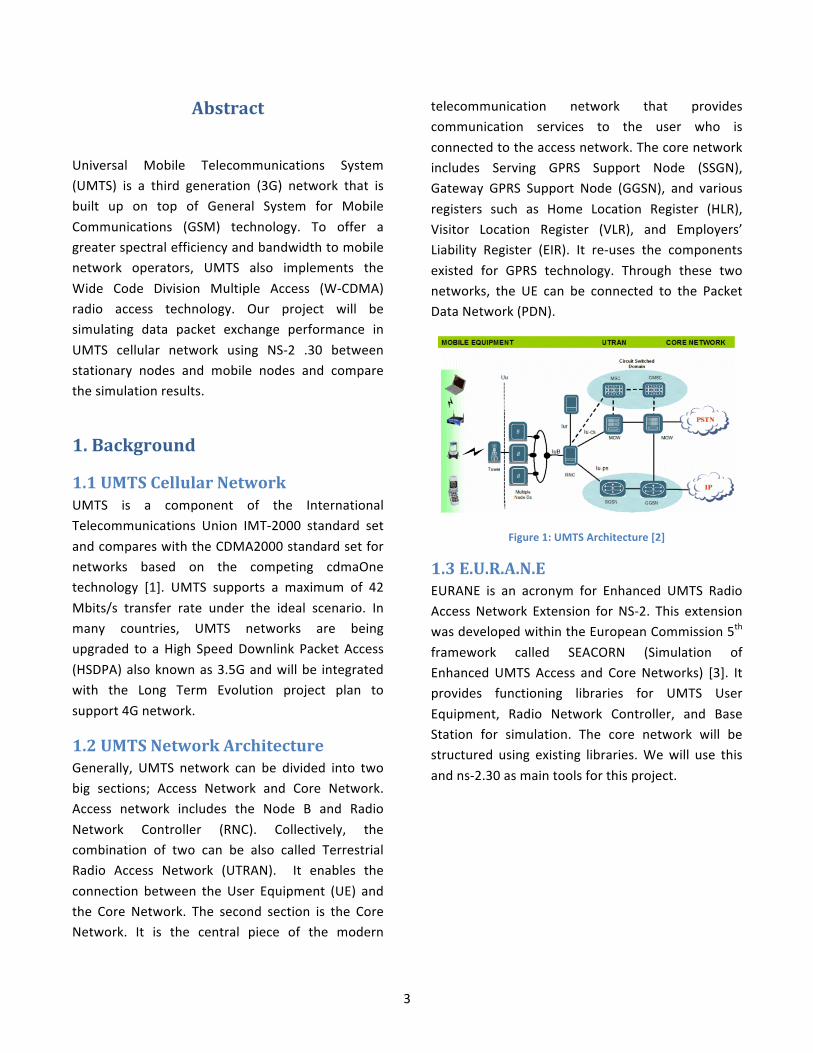
telecommunication network that provides communication services to the user who is connected to the access network. The core network includes Serving GPRS Support Node (SSGN), Gateway GPRS Support Node (GGSN), and various registers such as Home Location Register (HLR), Visitor Location Register (VLR), and Employers’ Liability Register (EIR). It re-‐uses the components existed for GPRS technology. Through these two networks, the UE can be connected to the Packet Data Network (PDN).
Figure 1: UMTS Architecture [2]
1.3 E.U.R.A.N.E EURANE is an acronym for Enhanced UMTS Radio Access Network Extension for NS-‐2. This extension was developed within the European Commission 5th framework called SEACORN (Simulation of Enhanced UMTS Access and Core Networks) [3]. It provides functioning libraries for UMTS User Equipment, Radio Network Controller, and Base Station for simulation. The core network will be structured using existing libraries. We will use this and ns-‐2.30 as main tools for this project.
4
2. Tools
2.1 NS-‐2 (Version 2.30) This is the main tool for our project, for simulating the CN architecture for both the UMTS and Wi-‐Fi scenarios.
2.2 E.U.R.A.N.E This tool is used for simulating the UMTS nodes including the Radio Network Controller (RNC), Base Station (BS) and User Equipment (UE) nodes.
2.3 Gnuplot Gnuplot is a command-‐line driven graphing tool, we are using it to plot all the results from the trace files for End-‐to-‐End delay and download bitrate.
2.4 MATLAB MATLAB is a tool for developing algorithms and analyzing data. We are using it to simulate a more realistic environment for the UEs. For example, as the UEs move away from the BS, there will be a bigger distortion in the End-‐to-‐End delay.
2.5 GAWK GAWK is for calculating the End-‐to-‐End Delay based on the trace files on each scenario. It creates a separate file to keep all the results.
3. UMTS
3.1 Implementation Universal Mobile Telecommunication System (UMTS) is a third generation mobile cellular technology. It utilizes existing Global System for Mobile Communications (GSM) standard for its core network. For our implementation, using NS-‐2, the core network was re-‐created with regular ns-‐2 node setup method; furthermore, the access network (consists of Radio Network Control (RNC), Base Station (BS), and User Equipment (UE)) was added
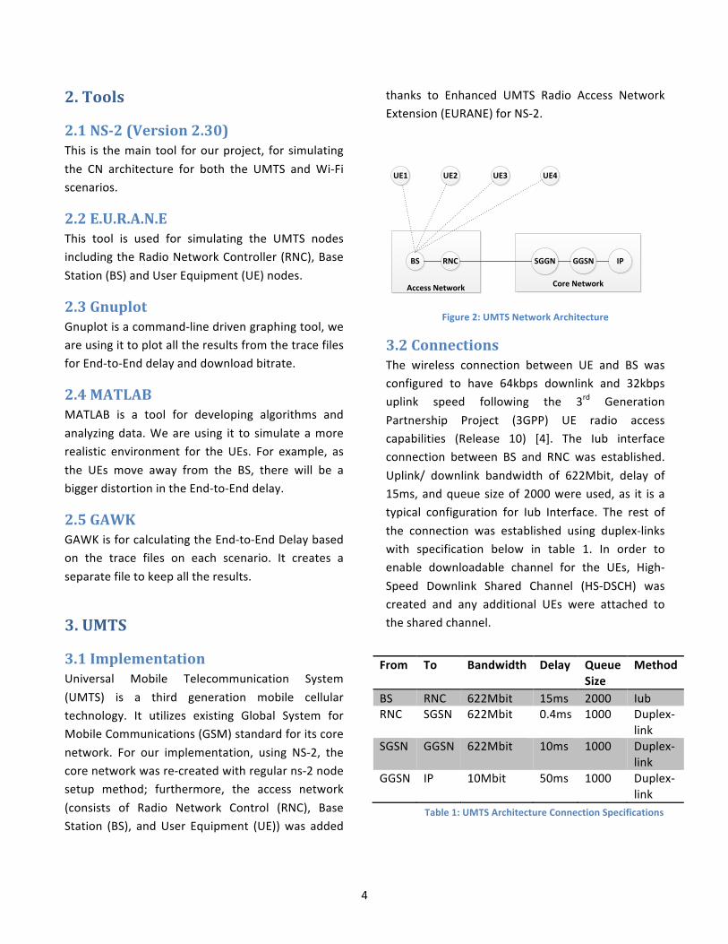
thanks to Enhanced UMTS Radio Access Network Extension (EURANE) for NS-‐2.
Access Network Core Network
BS RNC SGGN GGSN IP
UE1 UE2 UE3 UE4
Figure 2: UMTS Network Architecture
3.2 Connections The wireless connection between UE and BS was configured to have 64kbps downlink and 32kbps uplink speed following the 3rd Generation Partnership Project (3GPP) UE radio access capabilities (Release 10) [4]. The Iub interface connection between BS and RNC was established. Uplink/ downlink bandwidth of 622Mbit, delay of 15ms, and queue size of 2000 were used, as it is a typical configuration for Iub Interface. The rest of the connection was established using duplex-‐links with specification below in table 1. In order to enable downloadable channel for the UEs, High-‐Speed Downlink Shared Channel (HS-‐DSCH) was created and any additional UEs were attached to the shared channel.
From To Bandwidth Delay Queue Size
Method
BS RNC 622Mbit 15ms 2000 Iub RNC SGSN 622Mbit 0.4ms 1000 Duplex-‐
link SGSN GGSN 622Mbit 10ms 1000 Duplex-‐
link GGSN IP 10Mbit 50ms 1000 Duplex-‐
link Table 1: UMTS Architecture Connection Specifications
5
3.3 Scenario A UMTS network with specification configured as above was put to test with File Transfer Protocol (FTP) download performance. Over 100 seconds simulation time, packet sizes of 512 bytes was downloaded from IP to UE. Also after every 5 seconds, new UEs (Total of 4) were added to the simulation to observe any changes in the behaviour of the network throughput. The UEs were positioned at different distances from the BS to observe the behaviour as well.
3.4 Design Architecture Number of different tools was used in order to configure the simulation and obtain the desirable results. MATLAB script provided with the EURANE extension allowed us to configure the UEs via input trace files. Parameters such as distance from BS, speed, signal strength, and many other attributes could be configured. The input trace files were created for each UE and used from umts_proj.tcl. Also Signal-‐to-‐Noise Ratio file provided mimicked the noise in the simulation. Once the tcl script runs, it produces out_umts.tr and out_umts_ftp_download#.tr files. Out_umts_ftp_download#.tr (for 4 UEs) files were used directly by GNUPLOT to plot the measured download throughput of each UE node. For plotting the measured and calculated End-‐to-‐End delay wasn’t a simple task. The out_umts.tr containing all the trace information had to be analyzed with GAWK to produce a set of awk_eted#.tr to plot the End-‐to-‐End delay on each UE node. Finally, it can be plotted using the GNUPLOT.
3.5 Algorithms for Measuring Throughput and End-‐to-‐End Delay
The throughput was calculated in the tcl script that ran the whole simulation. The algorithm used here is referenced from the Marc Greis’ ns-‐2 tutorial. The time interval for measuring is 0.5 seconds. It sums
the numbers of bytes received by the sink (UE for our case) and then calculates the throughput based on the total bytes received in this time period. The current time and throughput are written to the trace file so we can plot them later using the GNUPLOT. The number of bytes received is reset to measure the throughput for the next cycle.
The End-‐to-‐End delay was obtained by selectively matching the flow identification to the node of interest. Once it matches, the algorithm checked the time when the packets were sent and received. Then the End-‐to-‐End delay is simply calculated by subtracting the time the packet was received by the time it was sent. It continues until the simulation ends. It was possible by using the GAWK script that allowed us to analyze the trace file a column by column.
ns-‐2
tcl
E.U.R.A.N.E
UE#_it (1,2,3,4)
MATLAB
umts_proj.tcl
out_umts_ftp_download#.tr (0,1,2,3)
out_umts.trGnuplot
graph_br.p graph_eted.p
GAWK
measure_eted#.awk (0,1,2,3)
awk_eted#.tr (0,1,2,3)
Results
SNRBLE Matrix
Figure 3: Design Architecture
4. Wi-‐Fi
4.1 Specification The IEEE 802.11 is a set of standards that governs the implementation, as well as identifying the medium access control (MAC) and physical layer (PHY) for the wireless local area network (WLAN). The 802.11a standard is one of the protocols in the 802.11 family. It is operated in the 5GHz frequency
6
range with a maximum data rate of 54Mbits/s. and uses a 52-‐subcarrier orthogonal frequency-‐division multiplexing (OFDM) [5]. The biggest advantage of using 802.11a is the low interference risk compared to other standards, such as 802.11b and 802.11g, which operates in the heavily crowded 2.4GHz frequency range. Compared to the 2.4GHz band, which is also shared by electronic devices, such as microwaves and Bluetooth, the 5GHz band sees much less interference. However, the high frequency also means that the range is relatively short, which is one of the disadvantages of using 802.11a standards.
4.2 System Design A simple 802.11 logical architecture contains several main components: a station, an access point (AP), a distribution system (DS), an extended service set (ESS), and an independent basic service set (IBSS). Moreover, there are two operating modes defined in 802.11: Ad-‐hoc mode and infrastructure mode.
The Ad-‐hoc mode, which is also called peer-‐to-‐peer mode, supports the stations to connect together when there is no AP present. The simple diagram is shown in the figure below [6].
Figure 4: Ad-‐hoc Network
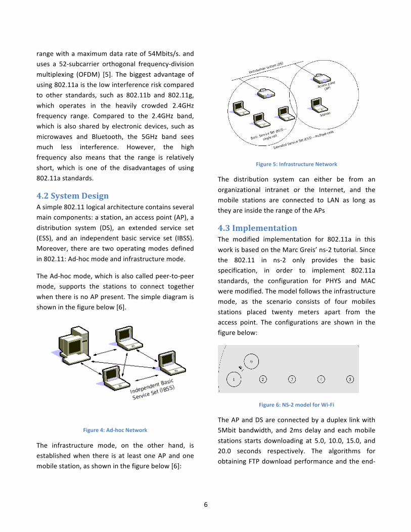
The infrastructure mode, on the other hand, is established when there is at least one AP and one mobile station, as shown in the figure below [6]:
Figure 5: Infrastructure Network
The distribution system can either be from an organizational intranet or the Internet, and the mobile stations are connected to LAN as long as they are inside the range of the APs
4.3 Implementation The modified implementation for 802.11a in this work is based on the Marc Greis’ ns-‐2 tutorial. Since the 802.11 in ns-‐2 only provides the basic specification, in order to implement 802.11a standards, the configuration for PHYS and MAC were modified. The model follows the infrastructure mode, as the scenario consists of four mobiles stations placed twenty meters apart from the access point. The configurations are shown in the figure below:
Figure 6: NS-‐2 model for Wi-‐Fi
The AP and DS are connected by a duplex link with 5Mbit bandwidth, and 2ms delay and each mobile stations starts downloading at 5.0, 10.0, 15.0, and 20.0 seconds respectively. The algorithms for obtaining FTP download performance and the end-‐
7
to-‐end delay for each mobile station were the same as in UMTS part.
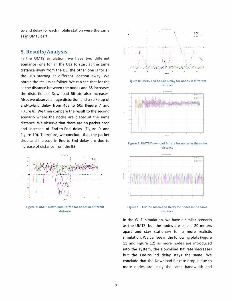
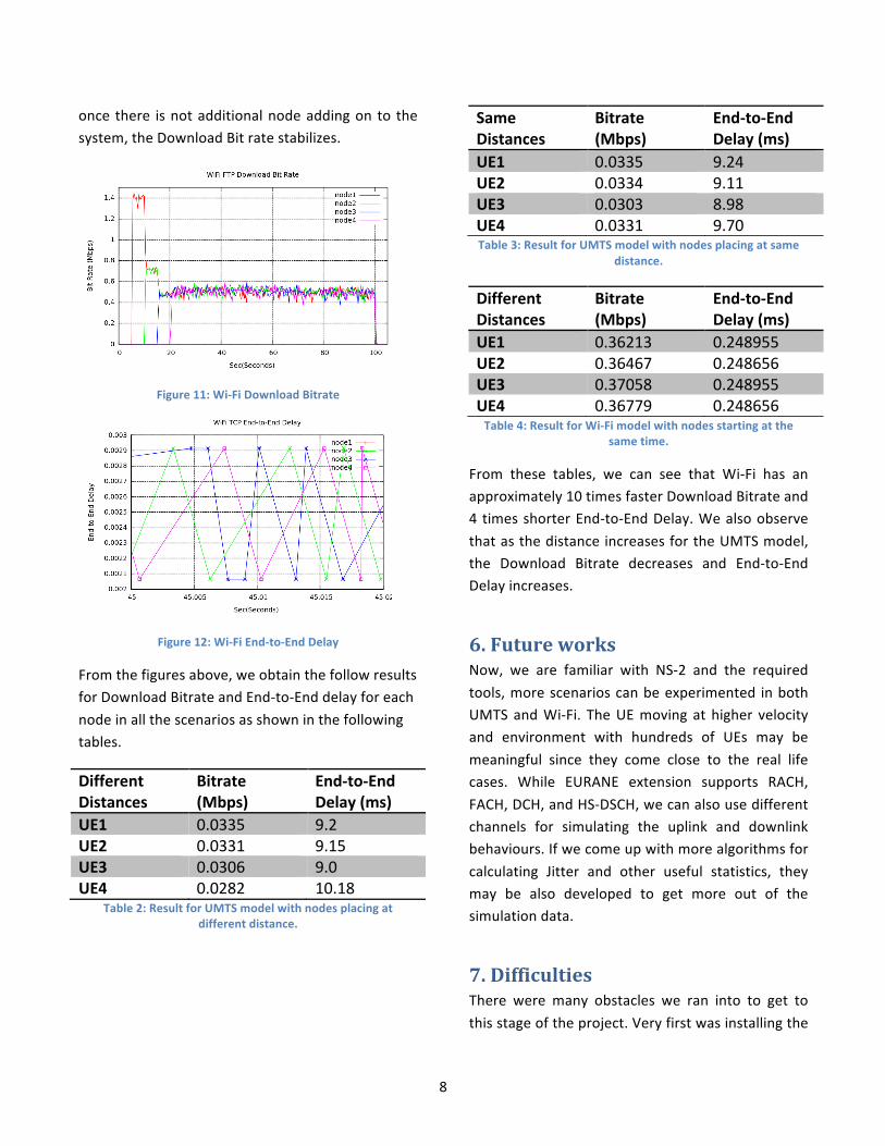
5. Results/Analysis In the UMTS simulation, we have two different scenarios, one for all the UEs to start at the same distance away from the BS, the other one is for all the UEs starting at different location away. We obtain the results as follow. We can see that for the as the distance between the nodes and BS increases, the distortion of Download Bitrate also increases. Also, we observe a huge distortion and a spike up of End-‐to-‐End delay from 40s to 50s (Figure 7 and Figure 8). We then compare the result to the second scenario where the nodes are placed at the same distance. We observe that there are no packet drop and increase of End-‐to-‐End delay (Figure 9 and Figure 10). Therefore, we conclude that the packet drop and increase in End-‐to-‐End delay are due to increase of distance from the BS.
Figure 7: UMTS Download Bitrate for nodes in different distance
Figure 8: UMTS End-‐to-‐End Delay for nodes in different distance
Figure 9: UMTS Download Bitrate for nodes in the same distance
Figure 10: UMTS End-‐to-‐End Delay for nodes in the same distance
In the Wi-‐Fi simulation, we have a similar scenario as the UMTS, but the nodes are placed 20 meters apart and stay stationary for a more realistic simulation. We can see in the following plots (Figure 11 and Figure 12) as more nodes are introduced into the system, the Download Bit rate decreases but the End-‐to-‐End delay stays the same. We conclude that the Download Bit rate drop is due to more nodes are using the same bandwidth and
8
once there is not additional node adding on to the system, the Download Bit rate stabilizes.
Figure 11: Wi-‐Fi Download Bitrate
Figure 12: Wi-‐Fi End-‐to-‐End Delay
From the figures above, we obtain the follow results for Download Bitrate and End-‐to-‐End delay for each node in all the scenarios as shown in the following tables.
Different Distances
Bitrate (Mbps)
End-‐to-‐End Delay (ms)
UE1 0.0335 9.2 UE2 0.0331 9.15 UE3 0.0306 9.0 UE4 0.0282 10.18
Table 2: Result for UMTS model with nodes placing at different distance.
Table 3: Result for UMTS model with nodes placing at same distance.
Table 4: Result for Wi-‐Fi model with nodes starting at the same time.
From these tables, we can see that Wi-‐Fi has an approximately 10 times faster Download Bitrate and 4 times shorter End-‐to-‐End Delay. We also observe that as the distance increases for the UMTS model, the Download Bitrate decreases and End-‐to-‐End Delay increases.
6. Future works Now, we are familiar with NS-‐2 and the required tools, more scenarios can be experimented in both UMTS and Wi-‐Fi. The UE moving at higher velocity and environment with hundreds of UEs may be meaningful since they come close to the real life cases. While EURANE extension supports RACH, FACH, DCH, and HS-‐DSCH, we can also use different channels for simulating the uplink and downlink behaviours. If we come up with more algorithms for calculating Jitter and other useful statistics, they may be also developed to get more out of the simulation data.
7. Difficulties There were many obstacles we ran into to get to this stage of the project. Very first was installing the
Same Distances
Bitrate (Mbps)
End-‐to-‐End Delay (ms)
UE1 0.0335 9.24 UE2 0.0334 9.11 UE3 0.0303 8.98 UE4 0.0331 9.70
Different Distances
Bitrate (Mbps)
End-‐to-‐End Delay (ms)
UE1 0.36213 0.248955 UE2 0.36467 0.248656 UE3 0.37058 0.248955 UE4 0.36779 0.248656

9
EURANE extension on top of NS-‐2. Installation of ns-‐2.30 on Ubuntu (Linux-‐based Platform) didn’t go as smooth as we though. Apparently, NS Animator (NAM) came with ns-‐2.30 all-‐in-‐one package was malfunctioning, so we had to install latest version of it to resolve the run-‐time compilation issues.
When the project script was up and running, the xgraph would not plot the trace files produced from the simulation. Because of this reason, we had to employee GNUPLOT to plot the valuable data. While the throughputs were calculated inside the script, End-‐to-‐End delay had to be calculated after analyzing the data with GAWK.
Most of tasks we did for this project required us to research and learn the new tools. Not many resources were available due to lack of interest on this topic in open source community, but we were able to manage our way by referring to relevant resources in different topics on NS-‐2. If we spent less time with the new tools, we could have used the time for analyzing the data obtained more in detail.
8. Conclusion This paper presents information about the performance of UMTS and Wi-‐Fi technologies in similar environment. NS-‐2 was the tool of the choice for simulating these communication technologies. Perhaps, it is impractical to compare such a different technology but we have learned to script in tcl and find a way through the project in Linux platform.
UMTS is a commonly used mobile technology for European countries. Based on the NS-‐2 simulation that we conducted for this technology, it is evident that the throughput is sensitive to the distance between UE and BS. The performance didn’t degrade with to the number of users connected to the system. We believe it is a correct behaviour for
a mobile network because it would not be acceptable to have the performance dropping due to the number of UE connected to it. Unfortunately, EURANE extension only supports single-‐cell environment, but it is clear that there is a need for hand-‐over to another cellular tower. Because when UE moves further away from the current service tower, the signal strength will likely to drop therefor more packet losses.
References [1] A.-‐C. Pang, J.-‐C. Chen, Y.-‐K. Chen, and P. Agrawal, “Mobility and Session Management: UMTS vs. CDMA2000,” IEEE Wireless Communications, Aug. 2004, pp. 30-‐43.
[2] OSS/BSS on UMTS Network UMTS architecture [Online]. Available: http://1.bp.blogspot.com/_Pf5g52hk3uw/S4HgRlEjCGI/AAAAAAAAAiY/hLXTpRmBd8o/s1600/RF_3G_OVERVW_UMTS_WIRELESS_NTWK.gif, Feb. 2010
[3] EURANE [Online]. Available: http://eurane.ti-‐wmc.nl/eurane/, Oct. 2006
[4] 3rd Generation Partnership Project, UE Radio Access Capabilities. Available: http://www.3gpp.org, Mar. 2012
[5] P. C. Mason, J. M. Cullen, and N. C. Lobley, “UMTS Architecture”, IEE Colloquium on Mobile Communications Towards the Next Millennium and Beyond, May 1996. London, UK.
[6] Wireless LAN (Wifi) Tutorial. Available: http://www.tutorial-‐reports.com/wireless/wlanwifi, Dec, 2007
[7] M. Vranjes, T. Svedek, and S. Imac-‐Drlje, “The Use of NS-‐2 Simulator in Studying UMTS Performances”, International Journal of Electrical and Computer Engineering Systems, Vol. 1, No. 2, Dec. 2010.

10
[8] N. R. Prasaad, “IEEE 802.11 System Design”, IEEE International Conference on Personal Wireless Communications, Dec. 2000, pp 490-‐494.
[9] Overview of the Universal Mobile Telecommunication System. Available online: http://www.umtsworld.com/technology/overview.htm, Jul. 2002
Appendix # # SPRING 2012 # # ENSC 427 -‐ Communications Network # # GROUP 5 PROJECT -‐ UMTS simulation in ns-‐2 # # utms_proj.tcl # global ns remove-‐all-‐packet-‐headers add-‐packet-‐header MPEG4 MAC_HS RLC LL Mac RTP TCP IP Common Flags set ns [new Simulator] set f [open trace_files/out_umts.tr w] $ns trace-‐all $f set f0 [open trace_files/out_umts_ftp_download0.tr w] set f1 [open trace_files/out_umts_ftp_download1.tr w] set f2 [open trace_files/out_umts_ftp_download2.tr w] set f3 [open trace_files/out_umts_ftp_download3.tr w] proc finish {} { global ns global f f0 f1 f2 f3 $ns flush-‐trace close $f close $f0 close $f1 close $f2 close $f3 puts " Simulation ended." # run the gnuplot # first is the bit rate graph exec gnuplot "graph_br.p" -‐persist & puts " BitRate Plotted." # second is the end-‐to-‐end delay graph puts " Calculating End-‐to-‐End Delay for UEs." exec gawk -‐f gawk/measure-‐eted0.awk "trace_files/out_umts.tr" exec gawk -‐f gawk/measure-‐eted1.awk "trace_files/out_umts.tr" exec gawk -‐f gawk/measure-‐eted2.awk "trace_files/out_umts.tr" exec gawk -‐f gawk/measure-‐eted3.awk "trace_files/out_umts.tr"
12
puts " Sorting End-‐to-‐End Delay Trace files." exec sort -‐n +0 -‐1 "trace_files/awk_eted0.tr" -‐o "trace_files/awk_eted0.tr" exec sort -‐n +0 -‐1 "trace_files/awk_eted1.tr" -‐o "trace_files/awk_eted1.tr" exec sort -‐n +0 -‐1 "trace_files/awk_eted2.tr" -‐o "trace_files/awk_eted2.tr" exec sort -‐n +0 -‐1 "trace_files/awk_eted3.tr" -‐o "trace_files/awk_eted3.tr" exec gnuplot "graph_eted.p" -‐persist & puts " End-‐to-‐End Delay Plotted." exit 0 } $ns set debug_ 0 $ns set hsdschEnabled_ 1 $ns set hsdsch_rlc_set_ 0 $ns set hsdsch_rlc_nif_ 0 ################################################################ # # Basic node configuration for UMTS Network Architecture # # [MS] [ AN ] [ CN ] # UE1 # \ # >-‐BS=RNC=SGSN=GGSN=node1=node2 # / # UE2 # . # . # UE3 # UE4 # # Legend: -‐ Wireless Connection # = Wired Connection # ################################################################ $ns node-‐config -‐UmtsNodeType rnc # Radio Network Control node address is 0. set rnc [$ns create-‐Umtsnode] $ns node-‐config -‐UmtsNodeType bs \ -‐downlinkBW 32kbs \ -‐downlinkTTI 10ms \ -‐uplinkBW 32kbs \ -‐uplinkTTI 10ms \ -‐hs_downlinkTTI 2ms \
13
-‐hs_downlinkBW 64kbs \ # Base Station node address is 1. set bs [$ns create-‐Umtsnode] # Setting up the Iub Interface between BS and RNC $ns setup-‐Iub $bs $rnc 622Mbit 622Mbit 15ms 15ms DummyDropTail 2000 $ns node-‐config -‐UmtsNodeType ue \ -‐baseStation $bs \ -‐radioNetworkController $rnc # Node address for ue1, ue2, ue3, and ue4 is 2, 3, 4, and 5 respectively. # note: only even number of ue nodes is supported. (known eurane bug) set ue1 [$ns create-‐Umtsnode] set ue2 [$ns create-‐Umtsnode] set ue3 [$ns create-‐Umtsnode] set ue4 [$ns create-‐Umtsnode] # Node address for sgsn0 and ggsn0 is 6 and 7, respectively. set sgsn0 [$ns node] set ggsn0 [$ns node] # Node address for node1 and node2 is 8 and 9, respectively. set node1 [$ns node] set node2 [$ns node] # Linking the access network and core network using the duplex links. $ns duplex-‐link $rnc $sgsn0 622Mbit 0.4ms DropTail 1000 $ns duplex-‐link $sgsn0 $ggsn0 622MBit 10ms DropTail 1000 $ns duplex-‐link $ggsn0 $node1 10MBit 15ms DropTail 1000 $ns duplex-‐link $node1 $node2 10MBit 35ms DropTail 1000 $rnc add-‐gateway $sgsn0 ############ Finished with Node Setup ########################## # added by DC # attach-‐ftp-‐traffic takes 5 parameters and then created a traffic between node and the sink. proc attach-‐ftp-‐traffic { node sink packetsize flowid priority } { #Get an instance of the simulator set ns [Simulator instance] global sink0 sink1 sink2 sink3 sink4 sink4 sink5 sink6 sink7 sink8 #Create a TCP agent and attach it set source [new Agent/TCP] $source set windowInit_ 10 $source set window_ 16
14
$source set packetSize_ $packetsize $source set fid_ $flowid $source set prio_ $priority $ns attach-‐agent $node $source #Create an FTP set traffic [new Application/FTP] $traffic attach-‐agent $source #Create a TCPSink set tcpsink [new Agent/TCPSink] $tcpsink set fid_ $flowid $ns attach-‐agent $sink $tcpsink $ns connect $source $tcpsink #hsdsch channel is created when ue1 connection is established #once the hsdsch channel is established, we ony need to attach any additional nodes. if {$flowid==0} { set sink0 $tcpsink $ns create-‐hsdsch $sink $tcpsink } if {$flowid==1} { set sink1 $tcpsink $ns attach-‐hsdsch $sink $tcpsink } if {$flowid==2} { set sink2 $tcpsink $ns attach-‐hsdsch $sink $tcpsink } if {$flowid==3} { set sink3 $tcpsink $ns attach-‐hsdsch $sink $tcpsink } return $traffic } # Process that records downlaod/upload bitrate # referenced from "Creating Output Files for Xgraph" tutorial proc record {} { global sink0 sink1 sink2 sink3 f0 f1 f2 f3 #Get an instance of the simulator set ns [Simulator instance] #Set the time after which the procedure should be called again set time 0.5 #How many bytes have been received by the traffic sinks?
15
set bw0 [$sink0 set bytes_] set bw1 [$sink1 set bytes_] set bw2 [$sink2 set bytes_] set bw3 [$sink3 set bytes_] #Get the current time set now [$ns now] #Calculate the bandwidth (in MBit/s) and write it to the files puts $f0 "$now [expr $bw0/$time*8/10000000]" puts $f1 "$now [expr $bw1/$time*8/10000000]" puts $f2 "$now [expr $bw2/$time*8/10000000]" puts $f3 "$now [expr $bw3/$time*8/10000000]" #Reset the bytes_ values on the traffic sinks $sink0 set bytes_ 0 $sink1 set bytes_ 0 $sink2 set bytes_ 0 $sink3 set bytes_ 0 #Re-‐schedule the procedure $ns at [expr $now+$time] "record" } ############ Configuring Tracing Setup ######################### # Following the specification from 3GPP TS 25.306 release 10 # http://www.3gpp.org/ftp/Specs/html-‐info/25306.htm $ns node-‐config -‐llType UMTS/RLC/AM \ -‐downlinkBW 64.0kbs \ -‐downlinkTTI 10ms \ -‐uplinkBW 64.0kbs \ -‐uplinkTTI 10ms \ -‐hs_downlinkTTI 2ms \ -‐hs_downlinkBW 128.0kbs # Creating and attaching HSDSCH and DCH for uplink and downlink # Please refer to eurane manual appendix D for schemetic view for different channels #channels will be created and attached in the attach-‐ftp-‐traffic proc # For FTP Downloading setup begins ############################# set source0 [attach-‐ftp-‐traffic $node2 $ue1 512 0 2] set source1 [attach-‐ftp-‐traffic $node2 $ue2 512 1 2] set source2 [attach-‐ftp-‐traffic $node2 $ue3 512 2 2] set source3 [attach-‐ftp-‐traffic $node2 $ue4 512 3 2] # For FTP Downloading setup finished ########################### # Configuring UEs' behaviours $bs setErrorTrace 0 "idealtrace_input/ue1_it" $bs setErrorTrace 1 "idealtrace_input/ue2_it"
16
$bs setErrorTrace 2 "idealtrace_input/ue3_it" $bs setErrorTrace 3 "idealtrace_input/ue4_it" $bs loadSnrBlerMatrix "misc/SNRBLERMatrix" #no need to setup dch (dedicated channel) since we are only measuring downlink. #set dch0 [$ns create-‐dch $ue1 $sink0] $ns at 0.0 "record" $ns at 5.0 "$source0 start" $ns at 10.0 "$source1 start" $ns at 15.0 "$source2 start" $ns at 20.0 "$source3 start" $ns at 100.0 "$source0 stop" $ns at 100.0 "$source1 stop" $ns at 100.0 "$source2 stop" $ns at 100.0 "$source3 stop" $ns at 100.5 "finish" puts " Simulation is running ... please wait ..." $ns run
17
# Wifi simulations # # wifi_proj.tcl # ====================================================================== # Define options # ====================================================================== set opt(chan) Channel/WirelessChannel ;# channel type set opt(prop) Propagation/TwoRayGround ;# radio-‐propagation model set opt(netif) Phy/WirelessPhy ;# network interface type set opt(mac) Mac/802_11 ;# MAC type set opt(ifq) Queue/DropTail/PriQueue ;# interface queue type set opt(ll) LL ;# link layer type set opt(ant) Antenna/OmniAntenna ;# antenna model set opt(ifqlen) 50 ;# max packet in ifq set opt(adhocRouting) NOAH ;# routing protocol (no ad-‐hoc) set opt(cp) "" ;# connection pattern file set opt(sc) "/home/andy/ns-‐allinone-‐2.30/ns-‐2.30/tcl/mobility/scene/scen-‐3-‐test" ;# node movement file. set opt(x) 600 ;# x coordinate of topology set opt(y) 600 ;# y coordinate of topology set opt(seed) 0.0 ;# seed for random number gen. # number of nodes set num_mobile_nodes 4 set num_wired_nodes 1 set num_bs_nodes 1 set num_total_nodes [expr $num_mobile_nodes + $num_mobile_nodes + $num_bs_nodes] remove-‐all-‐packet-‐headers add-‐packet-‐header MPEG4 MAC_HS RLC LL Mac RTP TCP IP Common Flags # 802.11a configurations Mac/802_11 set SlotTime_ 0.000050 ;# 50us Mac/802_11 set SIFS_ 0.000028 ;# 28us Mac/802_11 set PreambleLength_ 0 ;# no preamble Mac/802_11 set PLCPHeaderLength_ 128 ;# 128 bits Mac/802_11 set PLCPDataRate_ 1.0e6 ;# 1Mbps Mac/802_11 set dataRate_ 54.0e6 ;# 11Mbps Mac/802_11 set basicRate_ 1.0e6 ;# 1Mbps Phy/WirelessPhy set freq_ 5.0e+9 ;# 5GHz Phy/WirelessPhy set Pt_ 3.3962527e-‐2 ;# transmit power Phy/WirelessPhy set RXThresh_ 6.309573e-‐12 ;# receive sensitivity. Phy/WirelessPhy set CSThresh_ 6.309573e-‐12 # ============================================================================
18
# check for boundary parameters and random seed if { $opt(x) == 0 || $opt(y) == 0 } { puts "No X-‐Y boundary values given for wireless topology\n" } if {$opt(seed) > 0} { puts "Seeding Random number generator with $opt(seed)\n" ns-‐random $opt(seed) } # create simulator instance set ns [new Simulator] # set up for hierarchical routing $ns node-‐config -‐addressType hierarchical AddrParams set domain_num_ 2 ;# number of domains lappend cluster_num 2 1 ;# number of clusters in each domain AddrParams set cluster_num_ $cluster_num lappend eilastlevel 1 1 4 ;# number of nodes in each cluster AddrParams set nodes_num_ $eilastlevel ;# of each domain set tracefd [open trace_files/wifi_out.tr w] set namtrace [open wifi_out.nam w] # Create separate trace files for each node set f0 [open trace_files/wifi_out_node_0.tr w] set f1 [open trace_files/wifi_out_node_1.tr w] set f2 [open trace_files/wifi_out_node_2.tr w] set f3 [open trace_files/wifi_out_node_3.tr w] $ns trace-‐all $tracefd $ns namtrace-‐all $namtrace #$ns namtrace-‐all-‐wireless $namtrace $opt(x) $opt(y) # Create topography object set topo [new Topography] # Define topology $topo load_flatgrid $opt(x) $opt(y) # Create God create-‐god [expr $num_mobile_nodes + $num_bs_nodes] # Create wired nodes set temp {0.0.0 0.1.0} ;# hierarchical addresses for wired domain for {set i 0} {$i < $num_wired_nodes} {incr i} { set W($i) [$ns node [lindex $temp $i]] }
19
# Configure for base-‐station node $ns node-‐config -‐adhocRouting $opt(adhocRouting) \ -‐llType $opt(ll) \ -‐macType $opt(mac) \ -‐ifqType $opt(ifq) \ -‐ifqLen $opt(ifqlen) \ -‐antType $opt(ant) \ -‐propType $opt(prop) \ -‐phyType $opt(netif) \ -‐channelType $opt(chan) \ -‐topoInstance $topo \ -‐wiredRouting ON \ -‐agentTrace ON \ -‐routerTrace OFF \ -‐macTrace OFF #create base-‐station node set temp {1.0.0 1.0.1 1.0.2 1.0.3 1.0.4} ;# hier address to be used for wireless ;# domain set BS(0) [$ns node [lindex $temp 0]] $BS(0) random-‐motion 0 ;# disable random motion #provide some co-‐ord (fixed) to base station node $BS(0) set X_ 300.0 $BS(0) set Y_ 300.0 $BS(0) set Z_ 0.0 # create mobilenodes in the same domain as BS(0) # note the position and movement of mobilenodes is as defined # in $opt(sc) #configure for mobilenodes $ns node-‐config -‐wiredRouting OFF for {set j 0} {$j < $num_mobile_nodes} {incr j} { set mobile_node_($j) [ $ns node [lindex $temp \ [expr $j+1]] ] $mobile_node_($j) base-‐station [AddrParams addr2id \ [$BS(0) node-‐addr]] } # Create links between wired and BS nodes #$ns duplex-‐link $W(0) $W(0) 5Mb 2ms DropTail $ns duplex-‐link $W(0) $BS(0) 5Mb 2ms DropTail #$ns duplex-‐link-‐op $W(0) $W(0) orient down $ns duplex-‐link-‐op $W(0) $BS(0) orient left-‐down
20
# Set up TCP connections for each mobile node set tcp0 [new Agent/TCP] $tcp0 set windowInit_ 10 $tcp0 set window_ 16 $tcp0 set packetSize_ 512 $tcp0 set fid_ 0 $tcp0 set prio_ 0 set sink0 [new Agent/TCPSink] $sink0 set fid_ 0 $ns attach-‐agent $mobile_node_(0) $tcp0 $ns attach-‐agent $W(0) $sink0 $ns connect $tcp0 $sink0 set ftp0 [new Application/FTP] $ftp0 attach-‐agent $tcp0 set tcp1 [new Agent/TCP] $tcp1 set windowInit_ 10 $tcp1 set window_ 16 $tcp1 set packetSize_ 512 $tcp1 set fid_ 1 $tcp1 set prio_ 1 set sink1 [new Agent/TCPSink] $sink1 set fid_ 1 $ns attach-‐agent $mobile_node_(1) $tcp1 $ns attach-‐agent $W(0) $sink1 $ns connect $tcp1 $sink1 set ftp1 [new Application/FTP] $ftp1 attach-‐agent $tcp1 set tcp2 [new Agent/TCP] $tcp2 set windowInit_ 10 $tcp2 set window_ 16 $tcp2 set packetSize_ 512 $tcp2 set fid_ 2 $tcp2 set prio_ 2 set sink2 [new Agent/TCPSink] $sink2 set fid_ 2 $ns attach-‐agent $mobile_node_(2) $tcp2 $ns attach-‐agent $W(0) $sink2 $ns connect $tcp2 $sink2 set ftp2 [new Application/FTP] $ftp2 attach-‐agent $tcp2 set tcp3 [new Agent/TCP] $tcp3 set windowInit_ 10 $tcp3 set window_ 16 $tcp3 set packetSize_ 512

21
$tcp3 set fid_ 3 $tcp3 set prio_ 3 set sink3 [new Agent/TCPSink] $sink3 set fid_ 3 $ns attach-‐agent $mobile_node_(3) $tcp3 $ns attach-‐agent $W(0) $sink3 $ns connect $tcp3 $sink3 set ftp3 [new Application/FTP] $ftp3 attach-‐agent $tcp3 # source connection-‐pattern and node-‐movement scripts if { $opt(cp) == "" } { puts "*** NOTE: no connection pattern specified." set opt(cp) "none" } else { puts "Loading connection pattern..." source $opt(cp) } if { $opt(sc) == "" } { puts "*** NOTE: no scenario file specified." set opt(sc) "none" } else { puts "Loading scenario file..." source $opt(sc) puts "Load complete..." } # Define initial node position in nam for {set i 0} {$i < $num_mobile_nodes} {incr i} { # 20 defines the node size in nam, must adjust it according to your # scenario # The function must be called after mobility model is defined $ns initial_node_pos $mobile_node_($i) 5 } proc finish {} { global ns tracefd namtrace f0 f1 f2 f3 $ns flush-‐trace close $tracefd close $namtrace close $f0 close $f1 close $f2 close $f3 exec gnuplot "graph_bit_rate.p" -‐persist &
22
exec gawk -‐f gawk/wifi_delay_0.awk "trace_files/wifi_out.tr" exec gawk -‐f gawk/wifi_delay_1.awk "trace_files/wifi_out.tr" exec gawk -‐f gawk/wifi_delay_2.awk "trace_files/wifi_out.tr" exec gawk -‐f gawk/wifi_delay_3.awk "trace_files/wifi_out.tr" # sorts the time column for eted trace files exec sort -‐n +0 -‐1 "trace_files/awk_eted0.tr" -‐o "trace_files/awk_eted0.tr" exec sort -‐n +0 -‐1 "trace_files/awk_eted1.tr" -‐o "trace_files/awk_eted1.tr" exec sort -‐n +0 -‐1 "trace_files/awk_eted2.tr" -‐o "trace_files/awk_eted2.tr" exec sort -‐n +0 -‐1 "trace_files/awk_eted3.tr" -‐o "trace_files/awk_eted3.tr" exec gnuplot "graph_delay.p" -‐persist & exit 0 } proc record {} { global sink0 sink1 sink2 sink3 f0 f1 f2 f3 # Create simulator instance set ns [Simulator instance] # Set the time after which the procedure should be called set time 0.5 # Number of bytes received by the sink set bw0 [$sink0 set bytes_] set bw1 [$sink1 set bytes_] set bw2 [$sink2 set bytes_] set bw3 [$sink3 set bytes_] # Gets the current time set now [$ns now] # Calculate the BW (Mbits/s) and writes the output puts $f0 "$now [expr $bw0/$time*8/1000000]" puts $f1 "$now [expr $bw1/$time*8/1000000]" puts $f2 "$now [expr $bw2/$time*8/1000000]" puts $f3 "$now [expr $bw3/$time*8/1000000]" # Resets the number of bytes received by the sink $sink0 set bytes_ 0 $sink1 set bytes_ 0 $sink2 set bytes_ 0 $sink3 set bytes_ 0 # Re-‐schedule the procedure $ns at [expr $now + $time] "record"

23
} $ns at 0.0 "record" $ns at 5.0 "$ftp0 start" $ns at 10.0 "$ftp1 start" $ns at 15.0 "$ftp2 start" $ns at 20.0 "$ftp3 start" $ns at 100.0 "$ftp0 stop" $ns at 100.0 "$ftp1 stop" $ns at 100.0 "$ftp2 stop" $ns at 100.0 "$ftp3 stop" $ns at 105.0 "finish" puts "Starting Simulation..." $ns run
24
# wifi_delay_0.awk #This program is used to calculate the end-‐to-‐end delay for CBR BEGIN { highest_packet_id = 0; } { action = $1; time = $2; from = $3; to = $4; type = $5; pktsize = $6; flow_id = $8; src = $9; dst = $10; seq_no = $11; packet_id = $12; if ( type != "-‐-‐-‐" ) { if ( packet_id > highest_packet_id ) highest_packet_id = packet_id; if ( start_time[packet_id] == 0 ) start_time[packet_id] = time; # for fid_ 0 = node1 traffic if ( flow_id == 0 && action != "D" ) { if ( action == "r" ) { end_time[packet_id] = time; } } else { end_time[packet_id] = -‐1; } } } END { for ( packet_id = 0; packet_id < highest_packet_id; packet_id++ ) { start = start_time[packet_id]; end = end_time[packet_id]; packet_duration = end -‐ start; if ( start < end ) { printf("%f %f\n", start, packet_duration) > "trace_files/awk_eted0.tr"; }
25
} } # graph_delay.p set title "WiFi TCP End-‐to-‐End Delay" set autoscale unset log unset label set xtic auto set ytic auto set xlabel "Sec(Seconds) " set ylabel "End-‐to-‐End Delay" set xrange [45:45.02] set grid plot "trace_files/awk_eted0.tr" using 1:2 with linespoints title 'node1',\ "trace_files/awk_eted1.tr" using 1:2 with linespoints title 'node2',\ "trace_files/awk_eted2.tr" using 1:2 with linespoints title 'node3',\ "trace_files/awk_eted3.tr" using 1:2 with linespoints title 'node4' # graph_bit_rate.p set title "WiFi FTP Download Bit Rate" set autoscale unset log unset label set xtic auto set ytic auto set xlabel "Sec(Seconds) " set ylabel "Bit Rate (Mbps)" set xrange [0:105] set yrange [0:1.5] set grid set output "project_wifi_out.ps" plot "trace_files/wifi_out_node_0.tr" using 1:2 with lines title 'node1',\ "trace_files/wifi_out_node_1.tr" using 1:2 with lines title 'node2',\ "trace_files/wifi_out_node_2.tr" using 1:2 with lines title 'node3',\ "trace_files/wifi_out_node_3.tr" using 1:2 with lines title 'node4'


![SGSN-MME Combo Optimization - Cisco - Global Home …€¦ · lte-policy [no]sgsn-mmesubscriber-data-optimization end ... SGSN-MME Combo Optimization Monitoring Commands for the MME](https://img.pdfslide.us/doc/110x75/5acb94f17f8b9aa1518b52f6/sgsn-mme-combo-optimization-cisco-global-home-lte-policy-nosgsn-mmesubscriber-data-optimization.jpg)